Semiparametric empirical likelihood inference for abundance
from one-inflated capture–recapture data

Abstract

Abundance estimation from capture–recapture data is of great importance in many disciplines. Analysis of capture–recapture data is often complicated by the existence of one-inflation and heterogeneity problems. Simultaneously taking these issues into account, existing abundance estimation methods are usually constructed on the basis of conditional likelihood (CL) under one-inflated zero-truncated count models. However, the resulting Horvitz–Thompson-type estimators may be unstable, and the resulting Wald-type confidence intervals may exhibit severe undercoverage. In this paper, we propose a semiparametric empirical likelihood (EL) approach to abundance estimation under one-inflated binomial and Poisson regression models. We show that the maximum EL estimator for the abundance follows an asymptotically normal distribution and that the EL ratio statistic of abundance follows a limiting chi-square distribution with one degree of freedom. To facilitate computation of the EL method, we develop an expectation-maximization (EM) algorithm, and establish its appealing convergence property. We also propose a new score test for the existence of one-inflation and prove its asymptotic normality. Our simulation studies indicate that compared with CL-based methods, the maximum EL estimator has a smaller mean square error, the EL ratio confidence interval has a remarkable gain in coverage probability, and the proposed score test is more powerful. The advantages of the proposed approaches are further demonstrated by analyses of prinia data from Hong Kong and drug user data from Bangkok.

1 Introduction

Knowledge of the abundance of species or the sizes of hidden and elusive populations is of importance in ecology, epidemiology, public health, and social sciences (McCrea & Morgan, 2014; Böhning et al., 2017). For example, management of conservation is facilitated by data on population numbers of endangered species (Pérez et al., 2014), and details about increased numbers of unskilled immigrants may be important for income maintenance programs because of the resulting increased costs (Borjas, 1994). To estimate abundance, capture–recapture experiments constitute a widely used sampling technique for data collection (Otis et al., 1978). These experiments are based on a series of occasions or are conducted over a period of time, during which individuals are captured, marked or noted, and then released back into the population. The collected data usually exhibit two features: individual heterogeneity and one-inflation (Chao, 2001; Böhning et al., 2017; Godwin & Böhning, 2017).

Individual heterogeneity has been thought of as a key factor affecting the probability of being captured. Ignoring heterogeneity may lead to severely biased estimates (Chao, 2001). A number of nonparametric abundance estimators, which account for unobserved heterogeneity, have been proposed, such as the jackknife estimator (Burnham & Overton, 1978), the estimator of Zelterman (1988), and the lower bound estimator of Chao (1987). As individual covariates are usually available in practice, heterogeneity among capture probabilities could be modeled by parametric regression models on covariates, e.g., binomial regression models for discrete-time capture–recapture data and Poisson regression models for continuous-time capture–recapture data (Chao, 2001; van der Heijden et al., 2003). In the presence of individual covariates, researchers have developed partial likelihood, conditional likelihood (CL), and semiparametric empirical likelihood (EL) methods to make inference for abundance; see Huggins & Hwang (2011) and Liu et al. (2017, 2018). Maximum EL estimators of abundance usually have smaller mean square errors than CL-based estimators and EL ratio confidence intervals (CIs) have more accurate coverage probabilities than CL-based CIs.

One-inflation problems have recently received much attention in the context of capture–recapture models or zero-truncated count models. Godwin & Böhning (2017) first noticed that the number of captures usually exhibits a preponderance of “1”-counts. Ignoring excessive 1s may result in upwards biased estimates of population sizes. To account for the excess 1s, Godwin & Böhning (2017) proposed using a one-inflated zero-truncated Poisson distribution (see the model (6) in Section 3) and a zero-truncated one-inflated Poisson distribution (see the model (2) in Section 2.1) to model the probability mass function of the number of captures, and they suggested a score test for the one-inflation parameter. More complicated count models have been investigated in the literature, such as the one-inflated zero-truncated negative binomial model (Godwin, 2017; Inan, 2018), the one-inflated zero-truncated Poisson mixture model (Godwin, 2019), and the one-inflated zero-truncated geometric model (Böhning & van der Heijden, 2019; Böhning & Friedl, 2021). The zero-truncated one-inflated geometric model was also investigated in Chapter 14 of Böhning et al. (2017). Recently, Böhning & Ogden (2021) considered general count models allowing both inflation and deflation. Even though these models account for unobserved heterogeneity to some extent, quite a few researchers have resorted to regression models on individual covariates to characterize the heterogeneity among capture probabilities. As noted in the discussion sections of Böhning & van der Heijden (2019) and Böhning & Friedl (2021), the inclusion of covariates would be helpful to improve the fit of models and increase the likelihood of valid abundance predictions.

In this paper, we simultaneously consider the observed heterogeneity and one-inflation problems in the estimation of abundance from capture–recapture data. Under the one-inflated zero-truncated Poisson regression model, Godwin & Böhning (2017) proposed a Horvitz–Thompson-type estimator for the abundance and a CL-based score test for the one-inflation parameter. Under the one-inflated zero-truncated negative binomial regression model, Godwin (2017) also proposed a Horvitz–Thompson-type estimator and CL-based likelihood ratio tests for the one-inflation and unobserved heterogeneity. Inan (2018) further investigated the computation problem in terms of a mean-parameterized negative binomial distribution. However, the aforementioned methods have at least two limitations. First, Horvitz–Thompson-type estimators for abundance may be unstable if some detection probabilities are very close to zero. Meanwhile, variance estimations of these estimators have not been discussed. Second, these methods are inapplicable to the one-inflated zero-truncated binomial regression model and to zero-truncated one-inflated regression models.

We systematically study inference problems concerning abundance under “zero-truncated one-inflated” and “one-inflated zero-truncated” binomial and Poisson regression models, with available covariates incorporated in each model to explain the observed heterogeneity. Our contribution can be summarized as follows. First, for each considered model, we propose a new score test to test the existence of one-inflation. The score test statistic is derived from a full likelihood and is expected to be locally more powerful. Second, we extend the EL method for usual capture–recapture data to one-inflated capture–recapture data, with the resulting EL method inheriting the advantages over the CL method. Third, to maximize the EL function, we develop an efficient expectation-maximization (EM) algorithm, rather than using existing optimization functions such as the R function nlminb() adopted by Liu et al. (2017, 2018). The EM algorithm has an appealing convergence property and is free of Lagrange multipliers. Further, our numerical experience indicates that the estimation results from the EM algorithm are more stable and reliable than those derived from existing optimization functions in R.

The rest of the paper is organized as follows. In Section 2, we introduce the zero-truncated one-inflated regression models, and we present the semiparametric EL approach to abundance estimation and the score test for the one-inflation parameter. The EM algorithm is also discussed for numerical implementation. In Section 3, the proposed method and algorithm are extended to one-inflated zero-truncated regression models. In Section 4, several simulation studies are conducted to examine the finite-sample performance of the proposed methods. In Section 5, we apply the proposed approaches to two real-life data sets. Section 6 concludes with a discussion. For convenience of presentation, all proofs are given in the online Supporting Information.

2 Semiparametric empirical likelihood inference under zero-truncated one-inflated regression models

2.1 Model and data

Consider a closed population composed of $N$ individuals. For a generic individual, we denote by ${\bm{X}}$ and $Y$ the individual covariate and the number of times of being captured, respectively. Given ${\bm{X}}={\bm{x}}$, we assume that $Y$ follows a one-inflated count distribution with the conditional probability mass function

$$h(y,{\bm{x}};{\bm{\beta}},w)=wf(y,{\bm{x}};{\bm{\beta}})+(1-w)\cdot I(y=1).$$ (1)

Here $0\leq 1-w<1$ is the proportion of one-inflation among the individuals in the population and $f(y,{\bm{x}};{\bm{\beta}})$ is the probability mass function without one-inflation. Under the model (1), the conditional distribution of $Y=y$ for an individual whose covariate is ${\bm{x}}$ and who has been captured at least once is

$${\rm pr}(Y=y\mid{\bm{X}}={\bm{x}},Y>0)=\frac{1-w}{1-f(0,{\bm{x}};{\bm{\beta}})}\cdot I(y=1)+\frac{wf(y,{\bm{x}};{\bm{\beta}})}{1-f(0,{\bm{x}};{\bm{\beta}})}\cdot I(y\geq 1).$$ (2)

In (2), the count process has one-inflation first and then zero-truncation next. Hence, the model (2) is called the “zero-truncated one-inflated regression model.”

For discrete-time capture–recapture data, $f(y,{\bm{x}};{\bm{\beta}})$ is usually chosen to be a binomial distribution. That is, for $y=0,\ldots,K,$

$$f(y,{\bm{x}};{\bm{\beta}})={K\choose y}\{g({\bm{x}};{\bm{\beta}})\}^{y}\{1-g({\bm{x}};{\bm{\beta}})\}^{K-y},\quad\mbox{with}\quad g({\bm{x}};{\bm{\beta}})=\frac{\exp({\bm{\beta}}^{\mathrm{\scriptscriptstyle\top}}{\bm{x}})}{1+\exp({\bm{\beta}}^{\mathrm{\scriptscriptstyle\top}}{\bm{x}})},$$

where $K$ is the number of capture occasions. For continuous-time capture–recapture data, $f(y,{\bm{x}};{\bm{\beta}})$ can be chosen to be a Poisson distribution with probability mass function

$$f(y,{\bm{x}};{\bm{\beta}})=\frac{\{\lambda({\bm{x}};{\bm{\beta}})\}^{y}}{y!}\exp\{-\lambda({\bm{x}};{\bm{\beta}})\},\quad\lambda({\bm{x}};{\bm{\beta}})=\exp({\bm{\beta}}^{\mathrm{\scriptscriptstyle\top}}{\bm{x}}),\quad y=0,1,\ldots.$$

Suppose $\{({\bm{X}}_{i},Y_{i}):i=1,\dots,N\}$ are independent and identically distributed copies of $({\bm{X}},Y)$ for $N$ individuals in the population under study. Without loss of generality, we assume that the first $n$ individuals have been captured at least once and the last $N-n$ individuals have not been captured at all. For clarity, we denote the observations by $\{({\bm{X}}_{i}={\bm{x}}_{i},Y_{i}=y_{i}):i=1,\dots,n\}$. Our primary goal is to estimate the abundance $N$. Under a zero-truncated one-inflated regression model, we may wonder whether one-inflation does in fact exist. This leads to our second goal: testing $H_{0}:w=1$ under the model (1) or (2) based on the observed data. In the next subsection, we develop a semiparametric EL and take it as the foundation of our subsequent statistical inference.

2.2 Abundance estimation

Based on the observations, the full likelihood is

$${\rm pr}(n)\times\prod_{i=1}^{n}{\rm pr}({\bm{X}}_{i}={\bm{x}}_{i}\mid Y_{i}>0)\times\prod_{i=1}^{n}{\rm pr}(Y_{i}=y_{i}\mid{\bm{X}}_{i}={\bm{x}}_{i},Y_{i}>0).$$

Let $\alpha={\rm pr}(Y=0)$ denote the probability of an individual never being captured. The number of individuals captured, $n$, follows a binomial distribution $\mathrm{Bi}(N,1-\alpha)$. Therefore, the first term in the full likelihood is ${\rm pr}(n)={N\choose n}(1-\alpha)^{n}\alpha^{N-n}$. For the second and third terms, it follows from the Bayes’ rule that

$$\prod_{i=1}^{n}{\rm pr}({\bm{X}}_{i}={\bm{x}}_{i}\mid Y_{i}>0) = \prod_{i=1}^{n}\frac{{\rm pr}(Y_{i}>0\mid{\bm{X}}_{i}={\bm{x}}_{i}){\rm pr}({\bm{X}}_{i}={\bm{x}}_{i})}{1-\alpha},$$

and

$$\prod_{i=1}^{n}{\rm pr}(Y_{i}=y_{i}\mid{\bm{X}}_{i}={\bm{x}}_{i},Y_{i}>0) = \prod_{i=1}^{n}\frac{{\rm pr}(Y_{i}=y_{i}\mid{\bm{X}}_{i}={\bm{x}}_{i})}{{\rm pr}(Y_{i}>0\mid{\bm{X}}_{i}={\bm{x}}_{i})}.$$

Combining the above equations, we have the full likelihood

$${N\choose n}\alpha^{N-n}\times\prod_{i=1}^{n}{\rm pr}(Y_{i}=y_{i}\mid{\bm{X}}_{i}={\bm{x}}_{i})\times\prod_{i=1}^{n}{\rm pr}({\bm{X}}_{i}={\bm{x}}_{i}).$$

We use EL (Owen, 1988, 1990) to handle the nonparametric marginal distribution $F({\bm{x}})$ of ${\bm{X}}$. Following the principle of EL, we model $F({\bm{x}})$ by a discrete distribution $\sum_{i=1}^{n}p_{i}I({\bm{x}}_{i}\leq{\bm{x}})$, where $p_{i}\geq 0$ ($i=1,\dots,n$) and $\sum_{i=1}^{n}p_{i}=1$. After substituting $p_{i}={\rm pr}({\bm{X}}_{i}={\bm{x}}_{i})$ into the likelihood and taking the logarithm, we get the log-EL

$$\widetilde{\ell}(N,{\bm{\beta}},w,\alpha,\{p_{i}\})=\log{N\choose n}+(N-n)\log(\alpha)+\sum_{i=1}^{n}\log\{h(y_{i},{\bm{x}}_{i};{\bm{\beta}},w)\}+\sum_{i=1}^{n}\log(p_{i}).$$ (3)

Since $\alpha={\mathbb{E}}\{{\rm pr}(Y=0\mid{\bm{X}})\}$, it follows from the model (1) that a feasible constraint on $F$ or the $p_{i}$ is $\sum_{i=1}^{n}\{wf(0,{\bm{x}}_{i};{\bm{\beta}})-\alpha\}p_{i}=0.$ Using the method of Lagrange multipliers, the maximum of (3) is achieved at $p_{i}=n^{-1}[1+\xi\{wf(0,{\bm{x}}_{i};{\bm{\beta}})-\alpha\}]^{-1},\quad i=1,\dots,n.$ Substituting this equation into (3) gives the profile log-EL of $(N,{\bm{\beta}},w,\alpha)$:

$$\ell(N,{\bm{\beta}},w,\alpha)={} \log{N\choose n}+(N-n)\log(\alpha)+\sum_{i=1}^{n}\log\{h(y_{i},{\bm{x}}_{i};{\bm{\beta}},w)\}$$

$$-\sum_{i=1}^{n}\log[1+\xi\{wf(0,{\bm{x}}_{i};{\bm{\beta}})-\alpha\}]-n\log(n),$$ (4)

where $\xi=\xi({\bm{\beta}},w,\alpha)$ satisfies

$$\sum_{i=1}^{n}\frac{wf(0,{\bm{x}}_{i};{\bm{\beta}})-\alpha}{1+\xi\{wf(0,{\bm{x}}_{i};{\bm{\beta}})-\alpha\}}=0.$$

2.1

Under $H_{0}:w=1$, the model (1) or (2) degenerates to the case in which there is no one-inflation. In that situation, the semiparametric EL methods were first proposed by Liu et al. (2017) in discrete-time capture–recapture studies and then extended to continuous-time capture–recapture data by Liu et al. (2018). From this point of view, this paper can be seen as an extension of previous works to one-inflated capture–recapture data.

Based on the profile log-EL, we define the maximum EL estimator of $(N,{\bm{\beta}},w,\alpha)$ as $(\widehat{N},\widehat{\bm{\beta}},\widehat{w},\widehat{\alpha})=\arg\max_{(N,{\bm{\beta}},w,\alpha)}\{\ell(N,{\bm{\beta}},w,\alpha)\}$ and the EL ratio function of $N$ as $R(N)=2\{\ell(\widehat{N},\widehat{\bm{\beta}},\widehat{w},\widehat{\alpha})-\max_{({\bm{\beta}},w,\alpha)}\\ \ell(N,{\bm{\beta}},w,\alpha)\}.$ Before discussing the asymptotic behaviors of $(\widehat{N},\widehat{\bm{\beta}},\widehat{w},\widehat{\alpha})$ and the EL ratio statistic, we present an efficient numerical algorithm for implementing the EL methods.

2.3 EM algorithm

A key step in the implementation of the semiparametric EL method is to maximize the log-EL function (3) or the profile version (2.2). Similar to Liu et al. (2017) and Liu et al. (2018), one can maximize $\ell(N,{\bm{\beta}},w,\alpha)$ by using existing optimization functions such as the R function nlminb(). However, there is no theoretical guarantee that these functions work in the current setup. Further, when implementing the CL method in the absence of covariates, Godwin & Böhning (2017) noticed that their EM algorithm gives estimates with slightly less bias and smaller mean squared error, compared with those from packaged numerical methods. In this subsection, we develop an efficient EM algorithm for the numerical implementation of the proposed methods.

We first fix $N$, and we would like to maximize $\ell(N,{\bm{\beta}},w,\alpha)$ or $\widetilde{\ell}(N,{\bm{\beta}},w,\alpha,\{p_{i}\})$ with the given $N$. In this situation, there are two types of missing information in the context of the one-inflated capture–recapture data: (1) the covariates are missing if individuals are not captured at all; (2) it is not known whether the event that an individual was captured exactly once is attributed to the one-inflation or not. To describe the second type of missing data, we introduce a latent variable $Z_{i}$ for individual $i$ that follows $\mathrm{Bi}(1,w)$ and is independent of ${\bm{X}}_{i}$ ($i=1,\ldots,N$). Given ${\bm{X}}_{i}={\bm{x}}_{i}$, $Y_{i}$ is assumed to have a probability mass function $f(y,{\bm{x}}_{i};{\bm{\beta}})$ for $Z_{i}=1$ and follow a degenerate distribution at one for $Z_{i}=0$. By this assumption, $Z_{i}=1$ if the observed value of $Y_{i}$ is not equal to one.

Without loss of generality, we assume that $y_{1}=\dots=y_{m}=1$ and $y_{i}>1$ for $i=m+1,\dots,n$. Given $N$, we let ${\bm{O}}$ and ${\bm{O}}^{*}$ denote the observed data and missing data, respectively. Then, the complete data can be written as ${\bm{O}}\cup{\bm{O}}^{*}$:

$${{\bm{O}}}={} \{(Y_{i}=y_{i},{\bm{X}}_{i}={\bm{x}}_{i}):i=1,\dots,n\}\cup\{Y_{i}=0:i=n+1,\dots,N\}$$

$$\cup\{Z_{i}=1:i=m+1,\dots,N\},$$

$${{\bm{O}}^{*}}={} \{{\bm{X}}_{j}={\bm{x}}_{j}^{*},j=n+1,\dots,N\}\cup\{Z_{i}=z_{i}^{*}:i=1,\dots,m\},$$

where ${\bm{x}}_{j}^{*}$s stand for the unobserved covariates of the individuals never captured and $z_{i}^{*}$s stand for the latent variables indicating whether $y_{i}$ arises from $f(y,{\bm{x}}_{i};{\bm{\beta}})$ or not. Both the ${\bm{x}}_{j}^{*}$ and the $z_{i}^{*}$ serve in the role of missing data in the framework of the EM algorithm (Dempster et al., 1977). Based on $\bf O\cup O^{*}$, the complete-data likelihood is

$$\prod_{i=1}^{m}\{{\rm pr}(Y_{i}=y_{i}\mid{\bm{X}}_{i}={\bm{x}}_{i},Z_{i}=z_{i}^{*}){\rm pr}(Z_{i}=z_{i}^{*}){\rm pr}({\bm{X}}_{i}={\bm{x}}_{i})\}$$

$$\times\prod_{i=m+1}^{n}\{{\rm pr}(Y_{i}=y_{i}\mid{\bm{X}}_{i}={\bm{x}}_{i},Z_{i}=1){\rm pr}(Z_{i}=1){\rm pr}({\bm{X}}_{i}={\bm{x}}_{i})\}$$

$$\times\prod_{j=n+1}^{N}\{{\rm pr}(Y_{j}=0\mid{\bm{X}}_{j}={\bm{x}}_{j}^{*},Z_{j}=1){\rm pr}(Z_{j}=1){\rm pr}({\bm{X}}_{j}={\bm{x}}_{j}^{*})\}.$$

Let ${\bm{\theta}}=({\bm{\beta}},w,\alpha,\{p_{i}\})$. Recall that the EL method models $F({\bm{x}})$ as $F({\bm{x}})=\sum_{i=1}^{n}p_{i}I({\bm{x}}_{i}\leq{\bm{x}})$. That is, ${\bm{x}}_{j}^{*}$ is equal to one of the ${\bm{x}}_{i}$. Hence, the complete-data log-likelihood of ${\bm{\theta}}$ can be written as

$$\ell_{c}({\bm{\theta}}) = \sum_{i=1}^{m}[I(z_{i}^{*}=0)\log(1-w)+I(z_{i}^{*}=1)\log\{wf(y_{i},{\bm{x}}_{i};{\bm{\beta}})\}]+\sum_{i=1}^{n}\log(p_{i})$$

$$+\sum_{i=m+1}^{n}\log\{wf(y_{i},{\bm{x}}_{i};{\bm{\beta}})\}+\sum_{i=1}^{n}\sum_{j=n+1}^{N}[I({\bm{x}}_{j}^{*}={\bm{x}}_{i})\log\{wf(0,{\bm{x}}_{i};{\bm{\beta}})p_{i}\}].$$

The core of an EM algorithm is the EM iteration, which consists of an E-step and an M-step. These steps are iterated until convergence. Let ${\bm{\theta}}^{(0)}$ be the initial value of ${\bm{\theta}}$. For $r=1,2,\dots$, we denote by ${\bm{\theta}}^{(r)}=({\bm{\beta}}^{(r)},w^{(r)},\alpha^{(r)},\{p_{i}^{(r)}\})$ the value of ${\bm{\theta}}$ after $r$ rounds of EM iterations. In the E-step of the $(r+1)$th iteration, we need to calculate $Q({\bm{\theta}}|{\bm{\theta}}^{(r)})={\mathbb{E}}\{\ell_{c}({\bm{\theta}})|{{\bm{O}}},{\bm{\theta}}^{(r)}\}$. Given ${\bm{O}}$ and using ${\bm{\theta}}^{(r)}$ for ${\bm{\theta}}$, the conditional expectation of $I(z_{i}^{*}=1)$ for $i=1,\dots,m$ is

$$v_{i}^{(r)}={\mathbb{E}}\{I(z_{i}^{*}=1)\mid{{\bm{O}}},{\bm{\theta}}^{(r)}\} = \frac{{\rm pr}(Z_{i}=1,Y_{i}=1\mid{\bm{X}}_{i}={\bm{x}}_{i},{\bm{\theta}}={\bm{\theta}}^{(r)})}{{\rm pr}(Y_{i}=1\mid{\bm{X}}_{i}={\bm{x}}_{i},{\bm{\theta}}={\bm{\theta}}^{(r)})}$$

$$= \frac{w^{(r)}f(1,{\bm{x}}_{i};{\bm{\beta}}^{(r)})}{1-w^{(r)}+w^{(r)}f(1,{\bm{x}}_{i};{\bm{\beta}}^{(r)})},$$

and the conditional expectation of $I({\bm{x}}_{j}^{*}={\bm{x}}_{i})$ for $j=n+1,\dots,N$ and $i=1,\dots,n$ is

$${\mathbb{E}}\{I({\bm{x}}_{j}^{*}={\bm{x}}_{i})\mid{{\bm{O}}},{\bm{\theta}}^{(r)}\}={\rm pr}({\bm{X}}_{j}={\bm{x}}_{i}\mid Y_{j}=0,{\bm{\theta}}={\bm{\theta}}^{(r)})=\frac{w^{(r)}f(0,{\bm{x}}_{i};{\bm{\beta}}^{(r)})p_{i}^{(r)}}{\alpha^{(r)}},$$

where $\alpha^{(r)}=w^{(r)}\sum_{i=1}^{n}f(0,{\bm{x}}_{i};{\bm{\beta}}^{(r)})p_{i}^{(r)}$. Thus, the conditional expectation of the complete-data log-likelihood is

$$Q({\bm{\theta}}|{\bm{\theta}}^{(r)}) = \ell_{1}(w)+{\ell_{2}({\bm{\beta}})}+\ell_{3}(\{p_{i}\}),$$

where

$$\ell_{1}(w) = \sum_{i=1}^{n}(1-v_{i}^{(r)})\log(1-w)+\sum_{i=1}^{n}(v_{i}^{(r)}+u_{i}^{(r)})\log(w),$$

$$\ell_{2}({\bm{\beta}}) = \sum_{i=1}^{n}[v_{i}^{(r)}\log\{f(y_{i},{\bm{x}}_{i};{\bm{\beta}})\}+u_{i}^{(r)}\log\{f(0,{\bm{x}}_{i};{\bm{\beta}})\}],$$

$$\ell_{3}(\{p_{i}\}) = \sum_{i=1}^{n}(u_{i}^{(r)}+1)\log(p_{i}),$$

with $u_{i}^{(r)}=(N-n)w^{(r)}f(0,{\bm{x}}_{i};{\bm{\beta}}^{(r)})p_{i}^{(r)}/\alpha^{(r)}$ for $i=1,\dots,n$, and $v^{(r)}_{i}=1$ for $i=m+1,\dots,n$.

In the M-step of the $(r+1)$th iteration, we update ${\bm{\theta}}$ by ${\bm{\theta}}^{(r+1)}$, which maximizes $Q({\bm{\theta}}|{\bm{\theta}}^{(r)})$ with respect to ${\bm{\theta}}$ under the constraints

$$p_{i}\geq 0,\;i=1,\dots,n,\quad\sum_{i=1}^{n}p_{i}=1,\quad\sum_{i=1}^{n}\{wf(0,{\bm{x}}_{i};{\bm{\beta}})-\alpha\}p_{i}=0.$$

Since the three parts in $Q({\bm{\theta}}|{\bm{\theta}}^{(r)})$ are functions of $w$, ${\bm{\beta}}$, and $p_{i}$s, respectively, the M-step could be easily implemented through the following steps.

Step 1

Maximizing $\ell_{1}(w)$ gives the updated value of $w$: $w^{(r+1)}=\sum_{i=1}^{n}(v_{i}^{(r)}+u_{i}^{(r)})/\sum_{i=1}^{n}(1+u_{i}^{(r)}).$

Step 2

Update ${\bm{\beta}}$ to ${\bm{\beta}}^{(r+1)}$ by maximizing $\ell_{2}({\bm{\beta}})$. This can be implemented by fitting a generalized linear regression model to the data $\{(y_{1},{\bm{x}}_{1}),\dots,(y_{n},{\bm{x}}_{n}),(0,{\bm{x}}_{1}),\dots,(0,{\bm{x}}_{n})\}$, with the weights being $(v_{1}^{(r)},\dots,v_{n}^{(r)},u_{1}^{(r)},\dots,u_{n}^{(r)})$. For example, it can be easily done by invoking the R function glm() with the link function being “logit” for the binomial case and “log” for the Poisson case.

Step 3

Update the $p_{i}$ to the maximizer of $\ell_{3}(\{p_{i}\})$, namely, $p_{i}^{(r+1)}=(u_{i}^{(r)}+1)/\sum_{i=1}^{n}(u_{i}^{(r)}+1),\quad i=1,\dots,n.$

Step 4

Update $\alpha$ to $\alpha^{(r+1)}=w^{(r+1)}\sum_{i=1}^{n}f(0,{\bm{x}}_{i};{\bm{\beta}}^{(r+1)})p_{i}^{(r+1)}$.

We make several comments on the above EM algorithm. First, following the proof in Dempster et al. (1977), we can show that the log-EL $\widetilde{\ell}(N,{\bm{\beta}},w,\alpha,\{p_{i}\})$ in (3) does not decrease after each iteration. Further, note that $\widetilde{\ell}(N,{\bm{\beta}},w,\alpha,\{p_{i}\})\leq 0$. Thus, the sequence $({\bm{\beta}}^{(r)},w^{(r)},\alpha^{(r)},\{p_{i}^{(r)}\})$ eventually converges to a stationary point of $\widetilde{\ell}(N,{\bm{\beta}},w,\alpha,\{p_{i}\})$ for given $N$. Or, equivalently, the sequence $({\bm{\beta}}^{(r)},w^{(r)},\alpha^{(r)})$ converges to a stationary point of $\ell(N,{\bm{\beta}},w,\alpha)$ for given $N$. Second, in the M-step, the updated values of unknown parameters either have closed forms or can be easily obtained using existing R functions. This makes the EM algorithm very stable and flexible. Third, we stop the algorithm when the increment in the log-EL (3) after an iteration is no greater than, say, $10^{-5}$.

We now consider the case where $N$ is unknown and discuss the numerical calculation of $(\widehat{N},\widehat{\bm{\beta}},\widehat{w},\widehat{\alpha})$. The above EM algorithm can be easily adapted for this situation. We need two modifications. First, we set $u_{i}^{(r)}$ to $(N^{(r)}-n)w^{(r)}f(0,{\bm{x}}_{i};{\bm{\beta}}^{(r)})p_{i}^{(r)}/\alpha^{(r)}$ in the $(r+1)$th iteration. Second, we add a maximization step to update $N$ after Step 4 as follows.

Step 4^′

Update $N$ to $N^{(r+1)}$ by maximizing $\log{N\choose n}+(N-n)\log(\alpha^{(r+1)})$. This step can be implemented by using the existing R function optimize().

The following theorem summarizes the properties of the EM algorithm discussed above.

2.2

With the EM algorithms described above, we have for $r=0,1,\dots,$

1. $\widetilde{\ell}(N,{\bm{\beta}}^{(r+1)},w^{(r+1)},\alpha^{(r+1)},\{p_{i}^{(r+1)}\})\geq\widetilde{\ell}(N,{\bm{\beta}}^{(r)},w^{(r)},\alpha^{(r)},\{p_{i}^{(r)}\})$ when $N$ is fixed at each iteration;

2. $\widetilde{\ell}(N^{(r+1)},{\bm{\beta}}^{(r+1)},w^{(r+1)},\alpha^{(r+1)},\{p_{i}^{(r+1)}\})\geq\widetilde{\ell}(N^{(r)},{\bm{\beta}}^{(r)},w^{(r)},\alpha^{(r)},\{p_{i}^{(r)}\})$ when $N$ is updated at each iteration.

2.4 Asymptotic property

In this subsection, we present the asymptotic properties of the maximum EL estimator $(\widehat{N},\widehat{\bm{\beta}},\widehat{\alpha},\widehat{w})$ and the EL ratio statistic $R(N_{0})$. Before that, we need some notation. Let $(N_{0},{\bm{\beta}}_{0},w_{0},\alpha_{0})$ be the true value of $(N,{\bm{\beta}},w,\alpha)$ with $0<\alpha_{0}<1$ and $0<w_{0}\leq 1$. We use $e_{f}({\bm{x}};{\bm{\beta}})$ and $v_{f}({\bm{x}};{\bm{\beta}})$ to denote the conditional expectation and variance, respectively, of $Y$ conditional on ${\bm{X}}={\bm{x}}$. For any vector or matrix ${\bm{A}}$, we use ${\bm{A}}^{\otimes 2}$ to denote ${\bm{A}}{\bm{A}}^{\mathrm{\scriptscriptstyle\top}}$. Define $\varphi={\mathbb{E}}\{1-w_{0}f(0,{\bm{X}};{\bm{\beta}}_{0})\}^{-1}$ and

$${\bf W}=\left[\vbox{\hbox{\kern-1.15198pt\raise 0.0pt\hbox{\kern 276.48044pt}\kern-276.48044pt\vbox{\offinterlineskip\vbox{}}\kern-1.15198pt}}\right],$$

where ${\bf 0}$ is the zero vector, ${\rm V}_{11}=1-\alpha_{0}^{-1}$, ${\rm V}_{14}={\rm V}_{41}=\alpha_{0}^{-1}$, and

$${\bf V}_{22} = w_{0}{\mathbb{E}}\!\left[\frac{f(0,{\bm{X}};{\bm{\beta}}_{0})\{e_{f}({\bm{X}};{\bm{\beta}}_{0})\}^{2}{\bm{X}}^{\otimes 2}}{1-w_{0}f(0,{\bm{X}};{\bm{\beta}}_{0})}-v_{f}({\bm{X}};{\bm{\beta}}_{0}){\bm{X}}^{\otimes 2}\right.$$

$$\qquad\left.+\frac{(1-w_{0})f(1,{\bm{X}};{\bm{\beta}}_{0})\{1-e_{f}({\bm{X}};{\bm{\beta}}_{0})\}^{2}{\bm{X}}^{\otimes 2}}{1-w_{0}+w_{0}f(1,{\bm{X}};{\bm{\beta}}_{0})}\right],$$

$${\bf V}_{23} = {\bf V}_{32}^{\mathrm{\scriptscriptstyle\top}}={\mathbb{E}}\!\left[\frac{f(1,{\bm{X}};{\bm{\beta}}_{0})\{1-e_{f}({\bm{X}};{\bm{\beta}}_{0})\}{\bm{X}}}{1-w_{0}+w_{0}f(1,{\bm{X}};{\bm{\beta}}_{0})}-\frac{f(0,{\bm{X}};{\bm{\beta}}_{0})e_{f}({\bm{X}};{\bm{\beta}}_{0}){\bm{X}}}{1-w_{0}f(0,{\bm{X}};{\bm{\beta}}_{0})}\right],$$

$${\rm V}_{33} = {\mathbb{E}}\!\left[-\frac{\{1-f(1,{\bm{X}};{\bm{\beta}}_{0})\}^{2}}{1-w_{0}+w_{0}f(1,{\bm{X}};{\bm{\beta}}_{0})}-\frac{1-f(0,{\bm{X}};{\bm{\beta}}_{0})-f(1,{\bm{X}};{\bm{\beta}}_{0})}{w_{0}}+\frac{\{f(0,{\bm{X}};{\bm{\beta}}_{0})\}^{2}}{1-w_{0}f(0,{\bm{X}};{\bm{\beta}}_{0})}\right],$$

$${\bf V}_{24} = {\bf V}_{42}^{\mathrm{\scriptscriptstyle\top}}={\mathbb{E}}\!\left\{\frac{w_{0}f(0,{\bm{X}};{\bm{\beta}}_{0})e_{f}({\bm{X}};{\bm{\beta}}_{0}){\bm{X}}}{1-w_{0}f(0,{\bm{X}};{\bm{\beta}}_{0})}\right\},\quad{\bf V}_{25}={\bf V}_{52}^{\mathrm{\scriptscriptstyle\top}}=(1-\alpha_{0})^{2}{\bf V}_{24},$$

$${\rm V}_{34} = {\rm V}_{43}=-{\mathbb{E}}\!\left\{\frac{f(0,{\bm{X}};{\bm{\beta}}_{0})}{1-w_{0}f(0,{\bm{X}};{\bm{\beta}}_{0})}\right\},\quad{\rm V}_{35}={\rm V}_{53}=(1-\alpha_{0})^{2}{\rm V}_{34},$$

$${\rm V}_{44} = \varphi-\alpha_{0}^{-1},\quad{\rm V}_{45}={\rm V}_{54}=(1-\alpha_{0})^{2}\varphi,\quad{\rm V}_{55}=(1-\alpha_{0})^{4}\varphi-(1-\alpha_{0})^{3}.$$

In the following theorem, we discuss the asymptotic properties of $(\widehat{N},\widehat{\bm{\beta}},\widehat{w},\widehat{\alpha})$ and $R(N_{0})$ when there exists one-inflation under the model (1) or (2).

2.3

Suppose that $0<w_{0}<1$ and ${\bf W}$ is positive definite. As $N_{0}\to\infty,$ we have

1. $\sqrt{N_{0}}\{(\widehat{N}-N_{0})/N_{0},(\widehat{\bm{\beta}}-{\bm{\beta}}_{0})^{\mathrm{\scriptscriptstyle\top}},\widehat{w}-w_{0},\widehat{\alpha}-\alpha_{0}\}^{\mathrm{\scriptscriptstyle\top}}\overset{d}{\longrightarrow}{\rm N}({\bf 0},{\bf W}^{-1}),$ where $\overset{d}{\longrightarrow}$ denotes convergence in distribution;

2. $\sqrt{N_{0}}(\widehat{N}/N_{0}-1)\overset{d}{\longrightarrow}{\rm N}(0,\sigma^{2}),$ where

   $$\sigma^{2}=\varphi-1-\left[\vbox{\hbox{\kern-1.15198pt\raise 0.0pt\hbox{\kern 46.08006pt}\kern-46.08006pt\vbox{\offinterlineskip\vbox{}}\kern-1.15198pt}}\right]\left[\vbox{\hbox{\kern-1.15198pt\raise 0.0pt\hbox{\kern 46.08008pt}\kern-46.08008pt\vbox{\offinterlineskip\vbox{}}\kern-1.15198pt}}\right]^{-1}\left[\vbox{\hbox{\kern-1.15198pt\raise 0.0pt\hbox{\kern 23.04004pt}\kern-23.04004pt\vbox{\offinterlineskip\vbox{}}\kern-1.15198pt}}\right];$$

3. $R(N_{0})\overset{d}{\longrightarrow}\chi^{2}_{1},$ where $\chi^{2}_{1}$ stands for the chi-square distribution with one degree of freedom.

In part (b) of Theorem 2.3, $\sigma^{2}$ is usually unknown. To construct a consistent estimate for $\sigma^{2}$, we note that the ${\rm V}_{ij}$ and $\varphi$ can be expressed as ${\mathbb{E}}\{J({\bm{X}};{\bm{\beta}}_{0},w_{0},\alpha_{0})\}$ for some function $J$, for which a consistent estimator is $(\widehat{N})^{-1}\sum_{i=1}^{n}J({\bm{x}}_{i};\widehat{\bm{\beta}},\widehat{w},\widehat{\alpha})/\{1-\widehat{w}f(0,{\bm{x}}_{i};\widehat{\bm{\beta}})\}.$ A consistent estimator of $\sigma^{2}$ can therefore be obtained by replacing the ${\rm V}_{ij}$ and $\varphi$ by their respective estimators. We denote this estimator by $\widehat{\sigma}^{2}$.

With parts (b) and (c) in Theorem 2.3, we can construct an EL ratio CI and a Wald-type CI of $N$ as

$$\mathcal{I}_{1}=\{N:R(N)\leq\chi^{2}_{1}(1-a)\},\quad\mathcal{I}_{2}=\{N:(\widehat{N}-N)^{2}/(\widehat{N}\widehat{\sigma}^{2})\leq\chi^{2}_{1}(1-a)\},$$

where $\chi^{2}_{1}(1-a)$ is the $(1-a)$th quantile of the $\chi_{1}^{2}$ distribution. Even though both $\mathcal{I}_{1}$ and $\mathcal{I}_{2}$ have asymptotically correct coverage probabilities, our simulation studies show that the EL ratio CI $\mathcal{I}_{1}$ is usually superior to the Wald-type CI $\mathcal{I}_{2}$.

2.5 Score test for the existence of one-inflation

One problem of practical and scientific interest is whether one-inflation exists. Under the model (1) or (2), this is equivalent to testing whether $w=1$. We propose a score test based on the semiparametric EL in (2.2) for the null hypothesis $H_{0}:w=1$.

Let $(\widetilde{N},\widetilde{\bm{\beta}},\widetilde{\alpha})$ be the maximum EL estimator of $(N,{\bm{\beta}},\alpha)$ under $H_{0}$. Taking the partial derivative of $\ell(N,{\bm{\beta}},w,\alpha)$ with respect to $w$ at $w=1$, and replacing the unknown parameters by the corresponding maximum EL estimators under $H_{0}$, we obtain the score statistic $\partial\ell(\widetilde{N},\widetilde{\bm{\beta}},1,\widetilde{\alpha})/\partial w=U(\widetilde{N},\widetilde{\bm{\beta}}),$ where $U(N,{\bm{\beta}})=N-\sum_{i=1}^{m}\{f(1,{\bm{x}}_{i};{\bm{\beta}})\}^{-1}$. We refer to Section 2.3 of the Supporting Information for a detailed derivation of this statistic. Next, we study the properties of $U(\widetilde{N},\widetilde{\bm{\beta}})$ and use it to construct a score test for testing $H_{0}:w=1$.

Let $\sigma_{u}^{2}={\rm V}_{66s}-[1,\,{\bf V}_{s}^{\mathrm{\scriptscriptstyle\top}},\,0]{\bf W}_{s}^{-1}[1,\,{\bf V}_{s}^{\mathrm{\scriptscriptstyle\top}},\,0]^{\mathrm{\scriptscriptstyle\top}},$ where ${\rm V}_{66s}={\mathbb{E}}[\{f(1,{\bm{X}};{\bm{\beta}}_{0})\}^{-1}]-1$, ${\bf V}_{s}={\mathbb{E}}[\{1-e_{f}({\bm{X}};{\bm{\beta}}_{0})\}{\bm{X}}]$, and ${\bf W}_{s}$ is defined in Equation (7) of the Supporting Information.

2.4

Suppose that ${\rm V}_{66s}<\infty$ and the matrix ${\bf W}_{s}$ is positive definite. Then

1. ${\mathbb{E}}\{U(N_{0},{\bm{\beta}}_{0})\}\leq 0,$ with equality holding if and only if $w_{0}=1;$

2. under the null hypothesis $H_{0}:w=1,$ as $N_{0}\to\infty,$ $N_{0}^{-1/2}U(\widetilde{N},\widetilde{\bm{\beta}})\overset{d}{\longrightarrow}N(0,\sigma_{u}^{2}).$

To construct a score test based on $U(\widetilde{N},\widetilde{\bm{\beta}})$, we need a consistent estimator for $\sigma_{u}^{2}$. This can be achieved by techniques similar to those in deriving $\widehat{\sigma}^{2}$ in Section 2.4. We denote the resulting consistent estimator of $\sigma_{u}^{2}$ by $\widetilde{\sigma}_{u}^{2}$. With the results in Theorem 2.4 and $\widetilde{\sigma}_{u}^{2}$, our score test statistic for $H_{0}:w=1$ is defined as $S=U(\widetilde{N},\widetilde{\bm{\beta}})/\{\widetilde{N}^{1/2}\widetilde{\sigma}_{u}\},$ which converges in distribution to $N(0,1)$ under $H_{0}$. At significance level $a$, we reject the null hypothesis $H_{0}:w=1$ when $S\leq Z_{a}$, where $Z_{a}$ is the $a$th quantile of $N(0,1)$.

3 Extension to one-inflated zero-truncated regression models

The proposed semiparametric EL approach is so flexible that it is applicable not only to zero-truncated one-inflated regression models, but also to one-inflated zero-truncated regression models. Given ${\bm{X}}={\bm{x}}$, a one-inflated zero-truncated regression model assumes that the conditional probability mass function of $Y$ is

$$h_{e}(y,{\bm{x}};{\bm{\beta}},w)=\begin{cases}f(0,{\bm{x}};{\bm{\beta}}),&y=0,\\ (1-w)\{1-f(0,{\bm{x}};{\bm{\beta}})\}+wf(1,{\bm{x}};{\bm{\beta}}),&y=1,\\ wf(y,{\bm{x}};{\bm{\beta}}),&y>1,\end{cases}$$ (5)

where $f(y,{\bm{x}};{\bm{\beta}})$ is the probability mass function defined in Section 2.1 and $0\leq 1-w<1$ describes the proportion of one- and zero-inflation in the population under study. Under the model (5), the conditional distribution of $Y=y$ for an individual whose covariate is ${\bm{x}}$ and who has been captured at least once is

$${\rm pr}(Y=y\mid{\bm{X}}={\bm{x}},Y>0)=(1-w)\cdot I(y=1)+\dfrac{wf(y,{\bm{x}};{\bm{\beta}})}{1-f(0,{\bm{x}};{\bm{\beta}})}\cdot I(y\geq 1).$$ (6)

As discussed in Godwin & Böhning (2017), the expression in (6) looks as if the count process were first truncated at zero and then had one-inflation. Hence, we call the model (6) a “one-inflated zero-truncated regression model.” Note that $1-w$ also describes the proportion of individuals in the sample who learned avoidance ability at their first capture and thus were not captured subsequently.

With arguments similar to those in Section 2.2, we obtain the log-EL function, which has the same form as (3) with $h(y,{\bm{x}};{\bm{\beta}},w)$ replaced by $h_{e}(y,{\bm{x}};{\bm{\beta}},w)$. Under the model (5) or (6), the profile log-EL becomes

$$\ell_{e}(N,{\bm{\beta}},w,\alpha)={} \log{N\choose n}+(N-n)\log(\alpha)+\sum_{i=1}^{n}\log\{h_{e}(y_{i},{\bm{x}}_{i};{\bm{\beta}},w)\}$$

$$-\sum_{i=1}^{n}\log[1+\xi\{f(0,{\bm{x}}_{i};{\bm{\beta}})-\alpha\}],$$ (7)

where $\xi=\xi({\bm{\beta}},\alpha)$ satisfies

$$\sum_{i=1}^{n}\frac{f(0,{\bm{x}}_{i};{\bm{\beta}})-\alpha}{1+\xi\{f(0,{\bm{x}}_{i};{\bm{\beta}})-\alpha\}}=0.$$

Based on (3), we define the maximum EL estimator of $(N,{\bm{\beta}},w,\alpha)$ as $(\widehat{N}_{e},\widehat{\bm{\beta}}_{e},\widehat{w}_{e},\widehat{\alpha}_{e})=\arg\max_{(N,{\bm{\beta}},w,\alpha)}\\ \ell_{e}(N,{\bm{\beta}},w,\alpha)$ and the EL ratio function of $N$ as $R_{e}(N)=2\{\ell_{e}(\widehat{N}_{e},\widehat{\bm{\beta}}_{e},\widehat{w}_{e},\widehat{\alpha}_{e})-\max_{({\bm{\beta}},w,\alpha)}\ell_{e}(N,{\bm{\beta}},w,\alpha)\}.$ With slight modifications, the EM algorithm proposed in Section 2.3 can still be used to calculate the EL estimators. See Section 3 of the Supporting Information for details.

Similar to Section 2.5, we can construct a score test for $H_{0}:w=1$ based on (3). The difference between (2.2) and (3) lies in that the constraint of the Lagrange multiplier $\xi$ in (2.2) is related to the one-inflation parameter $w$, but the $\xi$ in (3) is not. This results in a different score function for the null hypothesis $H_{0}:w=1$:

$$U_{e}({\bm{\beta}}):=\frac{\partial\ell_{e}(N,{\bm{\beta}},1,\alpha)}{\partial w}=\sum_{i=1}^{n}\frac{\dot{h}_{e}(y;{\bm{x}}_{i};{\bm{\beta}},1)}{h_{e}(y;{\bm{x}}_{i};{\bm{\beta}},1)}=n-\sum_{i=1}^{m}\frac{1-f(0;{\bm{x}}_{i};{\bm{\beta}})}{f(1;{\bm{x}}_{i};{\bm{\beta}})}.$$

Since ${\bm{\beta}}$ is unknown, we estimate it by its maximum EL estimator $\widetilde{\bm{\beta}}$ under $H_{0}$ and obtain $U_{e}(\widetilde{\bm{\beta}})$.

To present some asymptotic properties of $U_{e}(\widetilde{\bm{\beta}})$, we define

where ${\rm V}_{66e}={\mathbb{E}}[\{1-f(0,{\bm{X}};{\bm{\beta}}_{0})\}^{2}\{f(1,{\bm{X}};{\bm{\beta}}_{0})\}^{-1}]-(1-\alpha_{0})$, ${\bf V}_{se}={\mathbb{E}}[\{1-f(0,{\bm{X}};{\bm{\beta}}_{0})-e_{f}({\bm{X}};{\bm{\beta}}_{0})\}{\bm{X}}]$, and

$${\bf V}_{26e}={\mathbb{E}}\!\left[\left\{\frac{e_{f}({\bm{X}};{\bm{\beta}}_{0})}{1-f(0,{\bm{X}};{\bm{\beta}}_{0})}-1+f(0,{\bm{X}};{\bm{\beta}}_{0})-f(0,{\bm{X}};{\bm{\beta}}_{0})e_{f}({\bm{X}};{\bm{\beta}}_{0})\right\}{\bm{X}}\right].$$

3.1

Let ${\bf W}_{e}$ and $\sigma_{e}^{2}$ be two quantities defined in Section 1.2 of the Supporting Information. Suppose that the matrices ${\bf W}_{s}$ and ${\bf W}_{e}$ are positive definite.

1. Assume $0<w_{0}<1$. As $N_{0}\to\infty,$ $\sqrt{N_{0}}\{(\widehat{N}_{e}-N_{0})/N_{0},(\widehat{\bm{\beta}}_{e}-{\bm{\beta}}_{0})^{\mathrm{\scriptscriptstyle\top}},\widehat{w}_{e}-w_{0},\widehat{\alpha}_{e}-\alpha_{0}\}^{\mathrm{\scriptscriptstyle\top}}\overset{d}{\longrightarrow}{\rm N}({\bf 0},{\bf W}_{e}^{-1}),$ $\sqrt{N_{0}}(\widehat{N}_{e}/N_{0}-1)\overset{d}{\longrightarrow}{\rm N}(0,\sigma_{e}^{2}),$ and $R_{e}(N_{0})\overset{d}{\longrightarrow}\chi^{2}_{1}$.

2. ${\mathbb{E}}\{U_{e}({\bm{\beta}}_{0})\}\leq 0,$ with equality holding if and only if $w_{0}=1$.

3. Under the null hypothesis $H_{0}:w=1,$ as $N_{0}\to\infty,$ $N_{0}^{-1/2}U_{e}(\widetilde{\bm{\beta}})\overset{d}{\longrightarrow}N(0,\sigma_{ue}^{2}).$

Using the technique to obtain $\widehat{\sigma}^{2}$ described in Section 2.4, we can similarly obtain consistent estimators (denoted by $\widehat{\sigma}_{e}^{2}$ and $\widetilde{\sigma}_{ue}^{2}$) for $\sigma_{e}^{2}$ and $\sigma_{ue}^{2}$. Based on part (a) of Theorem 3.1, we define the EL ratio confidence interval of $N$ as $\mathcal{I}_{1e}=\{N:R_{e}(N)\leq\chi^{2}_{1}(1-a)\}$ and the Wald-type confidence interval as $\mathcal{I}_{2e}=\{N:(\widehat{N}_{e}-N)^{2}/(\widehat{N}_{e}\widehat{\sigma}^{2}_{e})\leq\chi^{2}_{1}(1-a)\}.$ With parts (b) and (c) of Theorem 3.1 and $\widetilde{\sigma}_{ue}^{2}$, we define our score test statistic for $H_{0}:w=1$ as $S_{e}=U_{e}(\widetilde{\bm{\beta}})/(\widetilde{N}^{1/2}\widetilde{\sigma}_{ue}).$ As $\widetilde{\sigma}_{ue}$ is consistent, when $N_{0}$ is large, $S_{e}$ converges in distribution to ${\rm N}(0,1)$ under $H_{0}$. We reject the null hypothesis of $w=1$ when $S_{e}\leq Z_{a}$ at significance level $a$.

4 Simulation studies

In this section, we use simulation studies to illustrate the finite-sample performance of the proposed EL methods. We focus on Poisson regression models here. More simulation results under binomial regression models are given in Section 4 of the Supporting Information.

Let ${\bm{X}}=(1,X)^{\mathrm{\scriptscriptstyle\top}}$ denote the individual covariate, where $X\sim{\rm N}(18,5)$ mimics the covariate distribution in drug user data in Section 5. Given ${\bm{X}}={\bm{x}}$, we generate the number of captures from two scenarios.

1. $Y$ is generated from the one-inflated model (1), where $f(y,{\bm{x}};{\bm{\beta}})$ is a Poisson regression model with the true value of regression coefficients being ${\bm{\beta}}_{0}=(-1.5,0.1)^{\mathrm{\scriptscriptstyle\top}}$. In this scenario, the capture probability ranges from 74% to 92%.

2. This is the same as Scenario A except that $Y$ is generated from the model (5) with ${\bm{\beta}}_{0}=(-2.1,0.1)^{\mathrm{\scriptscriptstyle\top}}$. In this scenario, the capture probability is about 49%.

In each scenario, we set $N_{0}=50$, 100, and 500. Based on simulated data sets, we evaluate the performance of the EL-based score tests and compare the maximum EL estimators and EL ratio confidence intervals with those from existing methods.

4.1 Comparison of score tests for the existence of one-inflation

For the null hypothesis $H_{0}:w=1$, two EL-based score tests ($S$ and $S_{e}$) were derived in Sections 2.5 and 3. As discussed, these two score test statistics asymptotically follow a standard normal distribution. Below, we compare their finite-sample performance with the CL-based score test under the model (5) or (6), denoted by $S_{c}=U_{e}(\widetilde{\bm{\beta}}_{c})/(\widetilde{N}_{HT}^{1/2}\widetilde{\sigma}_{uc})$, where $\widetilde{\bm{\beta}}_{c}$ is the maximum CL estimator of ${\bm{\beta}}$ and $\widetilde{N}_{HT}$ is the Horvitz–Thompson-type estimator of $N$ proposed by Godwin & Böhning (2017), and $\widetilde{\sigma}_{uc}^{2}$ is the estimator of ${\mathbb{V}{\rm ar}}\{U_{e}(\widetilde{\bm{\beta}}_{c})\}/\widetilde{N}_{HT}$. At significance level $a$, we reject $H_{0}:w=1$ when $S_{c}\leq Z_{a}$ and define the $p$-value of $S_{c}$ as the value of the cumulative distribution function of $\mathrm{N}(0,1)$ at the observed value of $S_{c}$, rather than as half of the tail probability that $\chi^{2}_{1}$ is greater than the observed value of $S_{c}^{2}$ given in the code of Godwin & Böhning (2017).

We first check if the limiting distribution provides an accurate approximation to the finite-sample distributions of $S$, $S_{e}$, and $S_{c}$. For this purpose, we consider Scenarios A and B with $w_{0}=1$. In Table 1, we present the simulated type I error rates of $S$, $S_{e}$, and $S_{c}$ at significance levels 1%, 5%, and 10% based on 50,000 repetitions. Overall, the type I error rates of all three tests are much closer to the significance levels in Scenario A, where the capture probability is high. In Scenario B with $N_{0}=50$, the type I error rates of $S_{e}$ and $S_{c}$ are usually underestimated, and those of $S$ are slightly inflated. By contrast, they become very close to the nominal significance levels as $N_{0}$ increases to 500. In summary, the limiting distributions of both test statistics provide a satisfactory approximation to their finite-sample distributions under both scenarios when $N_{0}$ is large.

Table 1: Simulated type I error rates (%) of $S$, $S_{e}$, and $S_{c}$ at significance levels of 1%, 5%, and 10%

		$N_{0}=50$				$N_{0}=100$				$N_{0}=500$
Scenario	Level	1%	5%	10%		1%	5%	10%		1%	5%	10%
A	$S$	1.15	5.36	10.54		1.15	5.38	10.31		1.02	5.20	10.38
	$S_{e}$	0.79	4.13	8.43		0.90	4.56	8.94		0.92	4.80	9.75
	$S_{c}$	0.60	3.33	6.91		0.73	3.87	7.68		0.84	4.38	9.05
B	$S$	1.47	6.40	11.93		1.34	6.03	11.46		1.16	5.31	10.43
	$S_{e}$	0.64	3.48	7.37		0.81	4.08	8.55		0.98	4.65	9.30
	$S_{c}$	0.58	2.90	6.14		0.70	3.43	7.13		0.86	4.19	8.41

We now compare the powers of the three score tests under alternative models. In each scenario, we choose seven values of $w_{0}$ ranging from 0.3 to 0.9 in increments of 0.1. In Table 2, we present the simulated powers at a significance level of 5% based on 2000 repetitions. We can see that the powers of $S_{e}$ are close to or slightly higher than those of $S_{c}$ in most cases. This may be because they are derived from the same model and the scores of these two tests have the same closed form. Relatively, the CL-based score test $S_{c}$ is not quite stable, because 7% and 13% of the estimates $\widetilde{\sigma}_{u}^{2}$ are negative in Scenario B with $w_{0}=0.3$ and 0.4, respectively. For the score test $S$, its powers are comparable to those of the other two tests when $N_{0}$ is as large as 500. An interesting observation is that as $N_{0}$ decreases to 100 and further to 50, the score test $S$ derived from the model (1) always dominates the score tests $S$ and $S_{c}$ derived from the model (5) whenever the true data-generating model is (1) or (5). A possible reason is that the model (1) is more parsimonious than the model (5), and thus the observed data contain more information about the former model when the sample size is small.

Table 2: Simulated powers (%) of the score tests $S$, $S_{e}$, and $S_{c}$ at a significance level of 5%

		Scenario A							Scenario B
$N_{0}$	$w_{0}$	0.9	0.8	0.7	0.6	0.5	0.4	0.3	0.9	0.8	0.7	0.6	0.5	0.4	0.3
50	$S$	15	26	42	54	61	68	68	9	12	16	20	25	30	37
	$S_{e}$	12	21	36	46	54	61	62	5	7	9	11	14	16	17
	$S_{c}$	10	17	31	43	51	60	61	5	6	9	11	14	17	20
100	$S$	19	37	60	77	85	88	88	9	15	21	29	34	38	43
	$S_{e}$	15	33	55	71	82	87	88	5	10	15	21	26	30	34
	$S_{c}$	13	31	52	69	80	87	88	4	9	14	20	24	29	35
500	$S$	51	93	99	100	100	100	100	12	31	49	65	76	83	87
	$S_{e}$	49	92	99	100	100	100	100	10	29	46	63	76	84	87
	$S_{c}$	48	91	100	100	100	100	100	10	28	44	61	75	83	87

4.2 Comparison of abundance estimation

In each scenario, we let $w_{0}$ be equal to 0.5, 0.7, and 0.9. For abundance estimation, we compare the proposed maximum EL estimator $\widehat{N}_{\rm EL}$ ($\widehat{N}$ or $\widehat{N}_{e}$) with the Horvitz–Thompson-type estimator $\widetilde{N}_{{\rm HT}}$ and the maximum EL estimator $\widetilde{N}$ under models without one-inflation. In Table 3, we present the simulated means and relative mean square errors (the ratios of the mean square errors to $N_{0}$) of the three estimators based on 2000 repetitions.

Table 3: Simulated means and relative mean square errors (RMSEs) of the maximum EL estimators ($\widetilde{N}$ and $\widehat{N}_{EL}$) and the Horvitz–Thompson-type estimator $\widetilde{N}_{HT}$

			$N_{0}=50$				$N_{0}=100$				$N_{0}=500$
Scenario		$w_{0}$	0.5	0.7	0.9		0.5	0.7	0.9		0.5	0.7	0.9
A	Mean	$\widetilde{N}$	113	75	56		203	144	112		963	699	552
		$\widetilde{N}_{\rm HT}$	65	57	53		111	108	104		506	506	506
		$\widehat{N}_{\rm EL}$	56	52	50		105	103	101		503	503	502
	RMSE	$\widetilde{N}$	139	20	3		132	23	3		441	82	7
		$\widetilde{N}_{\rm HT}$	42	6	2		16	4	2		1	2	3
		$\widehat{N}_{\rm EL}$	18	4	2		10	3	2		1	2	2
B	Mean	$\widetilde{N}$	115	83	63		196	143	115		840	644	540
		$\widetilde{N}_{\rm HT}$	100	75	61		148	122	106		547	526	505
		$\widehat{N}_{\rm EL}$	80	66	56		133	114	102		530	515	498
	RMSE	$\widetilde{N}$	204	80	23		181	48	11		262	52	8
		$\widetilde{N}_{\rm HT}$	191	68	23		120	35	9		35	16	7
		$\widehat{N}_{\rm EL}$	104	49	17		87	28	8		28	14	7

Clearly, the maximum EL estimator $\widetilde{N}$ is severely upward-biased when one-inflation is ignored in the regression models. A possible explanation for this observation is that the one-inflation can be regarded as a limiting form of “trap-shyness,” and ignoring it may make us falsely believe that the sample is skewed toward those individuals with low capture probability. This also explains why the probability of never being captured is estimated to be higher than it should be, and hence why the abundance estimates are upward-biased.

After incorporating one-inflation parameters into the regression models, it can be seen that the proposed maximum EL estimator $\widehat{N}_{\rm EL}$ always has smaller bias and RMSE than the Horvitz–Thompson-type estimator $\widetilde{N}_{\rm HT}$, especially when $N_{0}=50$ and 100.

Next, we compare the performance of the EL ratio confidence interval $\mathcal{I}_{\rm EL}$ ($\mathcal{I}_{1}$ or $\mathcal{I}_{1e}$) and the Wald-type confidence interval $\mathcal{I}_{\rm Wald}$ ($\mathcal{I}_{2}$ or $\mathcal{I}_{2e}$). For this purpose, we present in Table 4 the coverage probabilities of their two- and one-sided confidence intervals at a level of 95%. For the two-sided confidence intervals, the coverage probability of $\mathcal{I}_{\rm EL}$ is very close to the nominal level, with the departure being at most 2%. Even though $\mathcal{I}_{\rm Wald}$ has an accurate two-sided coverage probability when $N_{0}=500$, it often produces severe undercoverage as $N_{0}$ is 100 or 50 with the largest undercoverage being 11% in Scenario B.

Table 4: Simulated coverage probabilities (%) of the EL ratio confidence interval $\mathcal{I}_{\rm EL}$ and the Wald-type confidence interval $\mathcal{I}_{\rm Wald}$ at a nominal level of 95%

			$N_{0}=50$				$N_{0}=100$				$N_{0}=500$
Scenario	Type	$w_{0}$	0.5	0.7	0.9		0.5	0.7	0.9		0.5	0.7	0.9
A	Two-sided	$\mathcal{I}_{\rm EL}$	94	96	96		94	95	96		95	95	95
		$\mathcal{I}_{\rm Wald}$	89	91	90		91	93	93		94	95	96
	Lower limit	$\mathcal{I}_{\rm EL}$	96	96	98		95	95	97		95	95	95
		$\mathcal{I}_{\rm Wald}$	100	100	100		100	100	99		99	100	100
	Upper limit	$\mathcal{I}_{\rm EL}$	93	95	94		94	95	95		95	95	95
		$\mathcal{I}_{\rm Wald}$	87	88	87		88	90	90		91	92	93
B	Two-sided	$\mathcal{I}_{\rm EL}$	96	97	97		96	97	97		94	95	96
		$\mathcal{I}_{\rm Wald}$	84	87	89		90	91	91		94	94	94
	Lower limit	$\mathcal{I}_{\rm EL}$	96	97	98		94	96	98		92	94	96
		$\mathcal{I}_{\rm Wald}$	100	100	100		100	100	100		100	100	100
	Upper limit	$\mathcal{I}_{\rm EL}$	96	96	95		96	97	95		96	95	95
		$\mathcal{I}_{\rm Wald}$	82	85	86		88	88	89		91	91	91

Finally, we display in Figure 1 the quantile–quantile (QQ) plots of the pivotal statistic $(\widehat{N}-N_{0})/\{(\widehat{N})^{1/2}\widehat{\sigma}\}$ and the EL ratio statistic $R(N_{0})$ with their limiting distribution quantiles in Scenario A with $N_{0}=50$ and $w_{0}=0.5$. The plots for the other scenarios are similar and are omitted. Clearly, the quantiles of $R(N_{0})$ are very close to those of the limiting standard chi-square distribution. However, the sampling quantiles of $(\widehat{N}-N_{0})/\{(\widehat{N})^{1/2}\widehat{\sigma}\}$ are generally smaller than the quantiles of the limiting standard normal distribution. This phenomenon would explain why $\mathcal{I}_{\rm EL}$ has more accurate coverage probabilities than $\mathcal{I}_{\rm Wald}$ and why the lower limits of $\mathcal{I}_{\rm Wald}$ often produce overcoverage but its upper limits often produce undercoverage.

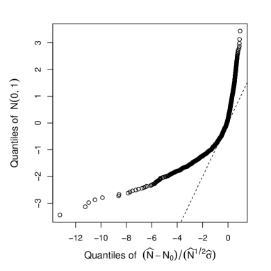
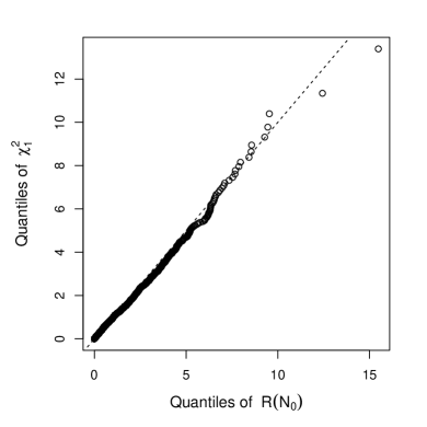
Figure 1: QQ plots of the pivotal statistic $(\widehat{N}-N_{0})/(\widehat{N}^{1/2}\widehat{\sigma})$ with the theoretical standard normal quantiles (left panel) and the empirical likelihood ratio $R(N_{0})$ with the theoretical $\chi^{2}_{1}$ quantiles (right panel). In both panels, the dashed line is the identity line.

5 Real data analysis

We further demonstrate the performance of the proposed EL-based score tests and abundance estimation methods by analyzing two real-life data sets: prinia data (Hwang & Huang, 2003; Liu et al., 2017) and drug user data (Böhning et al., 2004; Böhning & van der Heijden, 2009). The prinia data were collected at the Mai Po Bird Sanctuary in Hong Kong in 1993. Across 17 weekly capture occasions, 164 yellow-bellied prinia were captured at least once, and their wing lengths were measured. The drug user data concerned female methamphetamine users in Bangkok in 2001. In total, 274 drug users had contacted treatment institutions at least once, and their age information was collected. Here, the drug user was seen as being captured if she had contacted an institution once. To model the processes of being captured, we consider a binomial linear regression model and a Poisson linear regression model as $f(y,x;{\bm{\beta}})$ for the prinia data and drug user data, respectively.

5.1 Score tests for the existence of one-inflation

We first test whether or not there exists one-inflation among the number of captures. For this purpose, we perform the EL-based score tests $S$ under the zero-truncated one-inflated model (2) and $S_{e}$ under the one-inflated zero-truncated model (6). For the drug user data, both tests produce very small $p$-values, $4\times 10^{-4}$ for $S$ and $7\times 10^{-5}$ for $S_{e}$, which indicates that one-inflation does exist among the number of times that the drug users contacted the institutions.

The situation seems to be slightly different for the prinia data. The $p$-value of $S_{e}$ is 4.8%, which is very close to the significance level of 5%. However, the $p$-value of $S$ is 0.93%, which is strong evidence for the existence of one-inflation among the number of captures for the prinia data. From this, we argue that the EL-based score test $S$ under the model (2), is locally more powerful in detecting one-inflation than the test $S_{e}$ under the model (6).

5.2 Abundance estimation

In Table 5, we present the estimation results for the abundance of prinia and the total number of drug users. Clearly, there are striking differences between the maximum EL estimators $\widehat{N}_{\rm EL}$ and $\widetilde{N}$. Compared with $\widehat{N}_{\rm EL}$, ignoring the one-inflation problem usually makes the maximum EL estimator $\widetilde{N}$ and its standard error very large. We apply the CL-based method of Godwin & Böhning (2017) to the drug user data and obtainfor the Horvitz–Thompson-type estimator $\widetilde{N}_{\rm HT}$ a value of 307 under the model (2) and a value of 591 under the model (6). Consistent with the simulation results, $\widetilde{N}_{\rm HT}$ is often larger than $\widehat{N}_{\rm EL}$.

With regard to the confidence intervals of the abundance, we can see that the lower and upper limits of the Wald-type confidence interval $\mathcal{I}_{\rm Wald}$ are always lower than their counterparts for the EL ratio confidence interval $\mathcal{I}_{\rm EL}$. As discussed in the context of our simulation studies, the lower limit of the Wald-type confidence interval often produces severe overcoverage and its upper limit often produces undercoverage. In other words, the lower limit may be much conservative and the upper limit may lack some confidence. By contrast, the EL ratio confidence intervals could give more confidence.

Table 5: Maximum EL estimators ($\widetilde{N}$, $\widehat{N}_{\rm EL}$, $\widehat{w}$, and $\widehat{\omega}_{e}$) and their standard errors, together with the EL ratio and Wald-type confidence intervals of the abundance, for the prinia data and drug user data

Data	Model	$\widetilde{N}$	$\widehat{N}_{\rm EL}$	$\mathcal{I}_{\rm EL}$	$\mathcal{I}_{\rm Wald}$	$\widehat{w}$ or $\widehat{w}_{e}$
Prinia	(2)	484 (94)${\dagger}$	232 (49)	[181,499]	[137, 327]	0.66 (0.17)
	(6)	484 (94)	323 (75)	[226,594]	[175, 470]	0.58 (0.17)
Drug user	(2)	2725 (518)	295 (40)	[276, 483]	[216, 373]	0.18 (0.18)
	(6)	2725 (518)	554 (192)	[340, 1442]	[177, 931]	0.14 (0.07)

• The estimates of the standard errors of the maximum EL estimators are shown in parentheses.

We may wonder which of the models (2) and (6) fits the prinia data and the drug user data better. Table 6 presents the observed and fitted marginal frequencies of the numbers of captures in the real data sets. Let us take the model (2) and the prinia data as an example. We regard the observed and fitted marginal frequencies for the prinia data as a $2\times 5$ contingency table and use Pearson’s $\chi^{2}$ test statistic for independence in the contingency table to assess the goodness-of-fit of the model (2) for the prinia data. A smaller Pearson’s $\chi^{2}$ test statistic supports a better fit. Table 6 presents such test statistics for both of the models (2) and (6) and for both the real data sets. For the prinia data, Pearson’s $\chi^{2}$ test statistic (2.33) for the model (2) is smaller than that (2.74) for the model (6). This indicates that the zero-truncated one-inflated binomial regression model (2) fits the prinia data better. Similarly. the one-inflated zero-truncated Poisson regression model (6) fits the drug user data better.

Table 6: Observed and fitted marginal frequencies, together with the values of Pearson’s $\chi^{2}$ test statistic, for the number of captures in the prinia and drug user data

Data	Counts	1	2	3	4	5
Prinia	Observed	133	24	5	1	1
	Fitted (2)	134	23	7	2	0	$\chi^{2}=2.33$
	Fitted (6)	137	26	7	2	0	$\chi^{2}=2.74$
Drug user	Observed	261	10	2	1
	Fitted (2)	261	9	6	5		$\chi^{2}=5.58$
	Fitted (6)	263	10	6	4		$\chi^{2}=4.92$

6 Discussion

In this paper, we fit capture–recapture data by zero-truncated one-inflated and one-inflated zero-truncated Poisson and binomial regression models. More complicated count models have been investigated in the literature to account for unobserved heterogeneity in the context of one-inflated capture–recapture data (Godwin, 2017; Inan, 2018; Godwin, 2019; Böhning & Friedl, 2021). Taking the unobserved heterogeneity into account, we can alternatively define a geometric regression model with the “log” link as

$$f(y,{\bm{x}};{\bm{\beta}})=\left(\frac{\mu({\bm{x}};{\bm{\beta}})}{1+\mu({\bm{x}};{\bm{\beta}})}\right)^{y}\frac{1}{1+\mu({\bm{x}};{\bm{\beta}})},\quad\mu({\bm{x}};{\bm{\beta}})=\exp({\bm{\beta}}^{\mathrm{\scriptscriptstyle\top}}x),\quad\text{for }y=0,1,2,\dots.$$

Our semiparametric EL estimation procedure and the accompanying EM algorithm can be straightforwardly extended to deal with the one-inflated geometric regression model. In practice, some individual covariates are subject to missingness and measurement errors. Ignoring these two factors may lead to a biased abundance estimator (Stoklosa et al., 2019; Liu et al., 2020). Abundance estimation becomes much more challenging when capture–recapture data are contaminated missing data, one-inflation and zero-truncation. We leave this work for future research.

The research was supported by the China Postdoctoral Science Foundation (Grant 2020M681220), the National Natural Science Foundation of China (11771144), the State Key Program of National Natural Science Foundation of China (71931004 and 32030063), the Development Fund for Shanghai Talents, and the 111 project (B14019). The first three authors contributed equally to this paper.

Conflict of Interest

The authors have declared no conflict of interest.

Supporting Information

Additional supporting information may be found online in the Supporting Information section at the end of the article.

References

- Böhning & Friedl (2021) Böhning, D., & Friedl, H. (2021). Population size estimation based upon zero-truncated, one-inflated and sparse count data. Statistical Methods & Applications, . DOI: 10.1007/s10260-021-00556-8.
- Böhning & van der Heijden (2009) Böhning, D., & van der Heijden, P. G. M. (2009). A covariate adjustment for zero-truncated approaches to estimating the size of hidden and elusive populations. Annals of Applied Statistics, 3, 595–610.
- Böhning & van der Heijden (2019) Böhning, D., & van der Heijden, P. G. M. (2019). The identity of the zero-truncated, one-inflated likelihood and the zero-one-truncated likelihood for general count densities with an application to drink-driving in Britain. Annals of Applied Statistics, 13, 1198–1211.
- Böhning et al. (2017) Böhning, D., van der Heijden, P. G. M., & Bunge, J. (2017). Capture–Recapture Methods for the Social and Medical Sciences. New York: CRC.
- Böhning & Ogden (2021) Böhning, D., & Ogden, H. E. (2021). General flation models for count data. Metrika, 84, 245–261.
- Böhning et al. (2004) Böhning, D., Suppawattanabodee, B., Kusolvisitkul, W., & Viwatwongkasem, C. (2004). Estimating the number of drug users in Bangkok 2001: A capture–recapture approach using repeated entries in one list. European Journal of Epidemiology, 19, 1075–1083.
- Borjas (1994) Borjas, G. J. (1994). The economics of immigration. Journal of Economic Literature, 32, 1667–1717.
- Burnham & Overton (1978) Burnham, K. P., & Overton, W. S. (1978). Estimation of the size of a closed population when capture probabilities vary among animals. Biometrika, 65, 625–633.
- Chao (1987) Chao, A. (1987). Estimating the population size for capture–recapture data with unequal catchability. Biometrics, 43, 783–791.
- Chao (2001) Chao, A. (2001). An overview of closed capture–recapture models. Journal of Agricultural, Biological, and Environmental Statistics, 6, 158–175.
- Dempster et al. (1977) Dempster, A. P., Laird, N. M., & Rubin, D. B. (1977). Maximum likelihood from incomplete data via the EM algorithm. Journal of the Royal Statistical Society: Series B (Methodological), 39, 1–22.
- Godwin (2017) Godwin, R. T. (2017). One-inflation and unobserved heterogeneity in population size estimation. Biometrical Journal, 59, 79–93.
- Godwin (2019) Godwin, R. T. (2019). The one-inflated positive Poisson mixture model for use in population size estimation. Biometrical Journal, 61, 1541–1556.
- Godwin & Böhning (2017) Godwin, R. T., & Böhning, D. (2017). Estimation of the population size by using the one-inflated positive Poisson model. Journal of the Royal Statistical Society: Series C (Applied Statistics), 66, 425–448.
- van der Heijden et al. (2003) van der Heijden, P. G. M., Bustami, R., Cruyff, M. J., Engbersen, G., & van Houwelingen, H. C. (2003). Point and interval estimation of the population size using the truncated Poisson regression model. Statistical Modelling, 3, 305–322.
- Huggins & Hwang (2011) Huggins, R., & Hwang, W.-H. (2011). A review of the use of conditional likelihood in capture–recapture experiments. International Statistical Review, 79, 385–400.
- Hwang & Huang (2003) Hwang, W.-H., & Huang, S. Y. (2003). Estimation in capture–recapture models when covariates are subject to measurement errors. Biometrics, 59, 1113–1122.
- Inan (2018) Inan, G. (2018). One-inflation and unobserved heterogeneity in population size estimation by Ryan T. Godwin. Biometrical Journal, 60, 859–864.
- Liu et al. (2017) Liu, Y., Li, P., & Qin, J. (2017). Maximum empirical likelihood estimation for abundance in a closed population from capture–recapture data. Biometrika, 104, 527–543.
- Liu et al. (2018) Liu, Y., Liu, Y., Li, P., & Qin, J. (2018). Full likelihood inference for abundance from continuous time capture–recapture data. Journal of the Royal Statistical Society: Series B (Statistical Methodology), 80, 995–1014.
- Liu et al. (2020) Liu, Y., Liu, Y., Li, P., & Zhu, L. (2020). Maximum likelihood abundance estimation from capture–recapture data when covariates are missing at random. Biometrics, . DOI: 10.1111/biom.13334.
- McCrea & Morgan (2014) McCrea, R. S., & Morgan, B. J. (2014). Analysis of Capture–Recapture Data. Boca Raton, FL: Chapman and Hall/CRC.
- Otis et al. (1978) Otis, D. L., Burnham, K. P., White, G. C., & Anderson, D. R. (1978). Statistical inference from capture data on closed animal populations. Wildlife Monographs, 62, 3–135.
- Owen (1988) Owen, A. B. (1988). Empirical likelihood ratio confidence intervals for a single functional. Biometrika, 75, 237–249.
- Owen (1990) Owen, A. B. (1990). Empirical likelihood ratio confidence regions. Annals of Statistics, 18, 90–120.
- Pérez et al. (2014) Pérez, T., Naves, J., Vázquez, J. F., Fernández-Gil, A., Seijas, J., Albornoz, J., Revilla, E., Delibes, M., & Domínguez, A. (2014). Estimating the population size of the endangered cantabrian brown bear through genetic sampling. Wildlife Biology, 20, 300–309.
- Stoklosa et al. (2019) Stoklosa, J., Lee, S.-M., & Hwang, W.-H. (2019). Closed-population capture–recapture models with measurement error and missing observations in covariates. Statistica Sinica, 29, 589–610.
- Zelterman (1988) Zelterman, D. (1988). Robust estimation in truncated discrete distributions with application to capture–recapture experiments. Journal of Statistical Planning and Inference, 18, 225–237.