Dynamic off-the-grid untangling of curves with Reeds-Shepp metric.

Abstract

We propose an improved strategy for point sources tracking in a temporal stack through an off-the-grid fashion, inspired by the Benamou-Brenier regularisation in the literature. We define a lifting of the problem in the higher-dimensional space of the roto-translation group. This allows us to overcome the theoretical limitation of the off-the-grid method towards tangled point source trajectories, thus enabling the reconstruction and untangling even from the numerical standpoint. We define accordingly a new regularisation based on the relaxed Reeds-Shepp metric, an approximation of the sub-Riemannian Reeds-Shepp metric, further allowing control on the local curvature of the recovered trajectories. Then, we derive some properties of the discretisation and prove a $\Gamma$-convergence result, fostering interest for practical applications of polygonal, Bézier, and piecewise geodesic discretisation. We finally test our proposed method on a localisation problem example, and give a fair comparison with the state-of-the-art off-the-grid method.

46E27, 49N45, 53C80, 53C21, 58E30, 34K29.

1 Introduction and contributions

This work focuses on the definition of an off-the-grid framework, especially with an energy able to track crossing point sources from a temporal stack of measurements. In the context of inverse problem, this amounts to the recovery of crossing Dirac measures trajectories, also called dynamic Dirac measures. Such interest is motivated by the latest refinements in the off-the-grid community [9, 10, 25], where several results, such as an energy for moving point trajectories recovery and numerical implementation were enabled. It caters for both balanced (constant amplitude over time) and unbalanced (fluctuating amplitude) cases.

However, the literature in calculus of variations nowadays does not offer a genuine tractable off-the-grid framework for tangled paths: for instance, if two spikes are crossing, the current state-of-the-art cannot tackle these reconstructions and, on the contrary, yield two separate paths, which do not touch in any way. Yet such situations arise naturally in several domains such as biomedical imaging, where the physical objects used for super-resolution such as air bubbles can cross. An example of curves encountered in a natural and practical setting is presented in Figure 1.

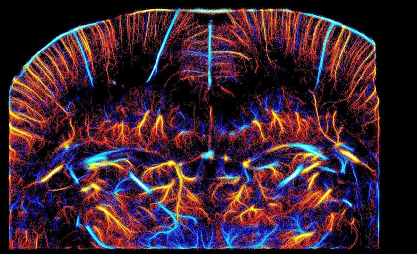
Figure 1: Crossing curves arise genuinely in several biological structures, such as cell nucleus, blood vessels, etc. This image is a reconstruction of blood vessels in a rat brain, performed by ULM (Ultrasound Localisation Microscopy) as joint work from ESPCI, Inserm and CNRS [26]. Color relates to the velocimetry of the microbubbles, red indicates high positive velocity while blue corresponds to high negative velocities.

In the following, we propose a method to recover the point sources paths, even when a crossing occurs. Our main idea boils down to a lifting on the roto-translation space [15, 23], see Figure 2, while formulating a new energy with a Riemannian regularisation tailored for paths untangling. Additionally, we propose a general theoretical framework for the numerical aspects, which proves convergence of the discretised problem towards the continuous problem, with a reduced set of hypothesis. To the best knowledge of the authors, this is the first attempt to recover tangled paths as dynamic Dirac measures, in an off-the-grid manner.

We will consider an inverse problem model similar to the one proposed in [39, 11] for which [25] added numerous numerical recipes. The main idea to solve this inverse problem in an off-the-grid fashion boils down to the reconstruction of a Radon measure supported on a space of curves. The reconstruction is achieved by minimising an energy functional with a data term that penalises distance between data and the candidate minimiser, and a regularisation term that is linear w.r.t. the candidate. Such formulation dictactes by design the shape of the minimisers: indeed, this problem was derived while having in mind the opportunity to use a representer theorem as the ones proven in [5, 7]. It provides a strong result as it ensures that the shape of the minimiser is determined by the extremal points of the unit ball of the regulariser; hence being able to characterise sharply the solution, as an a priori, before even solving the inverse problem. The representer theorem requires some few hypotheses, among which are the finite-dimensionality of the space on which the distance to data is computed. In [7], the authors give a proof that the extremal points of the unit ball for the considered Benamou-Brenier regularisation are Dirac measures on the space of curves, thus ensuring the sparsity and the shape of the solution. One may note that if [7] and [9] express the problem in terms of a time-dependent density $\rho(x,t)$ (represented as a measure-valued continuous function of time) and a velocity field $v_{t}$, coupled via the continuity equation, the solution realises the optimal transport between two marginal distributions, hence could be described by a path $\gamma$. Even if the correspondence is not one-to-one, one can associate a measure path $\delta_{\gamma}$ to a density $\rho(x,t)$ and velocity field $v_{t}$ couple, and conversely, at least under suitable smoothness conditions.

On the numerical side, a few works have been trying to propose numerical methods to recover curves from a temporal series of measurements, or stack of images. For instance, [10] proposes a conditional gradient method or Frank-Wolfe algorithm [28] to solve the considered inverse problem. Frank-Wolfe type algorithms are typical greedy algorithms deployed on a convex optimisation problem on a compact set, it consists of iteratively minimising the linearised version of the objective function on a compact set. Classic theory tells us that such minimisers will be located on extremal points of this compact set. The latest developments [25] expand on the Frank-Wolfe algorithm setup and leverage a dynamical programming approach to speed up the computation. They also extend the numerics to the ’unbalanced’ case, where each curve has an associated time-dependent amplitude, accounting for mass creation and destruction.

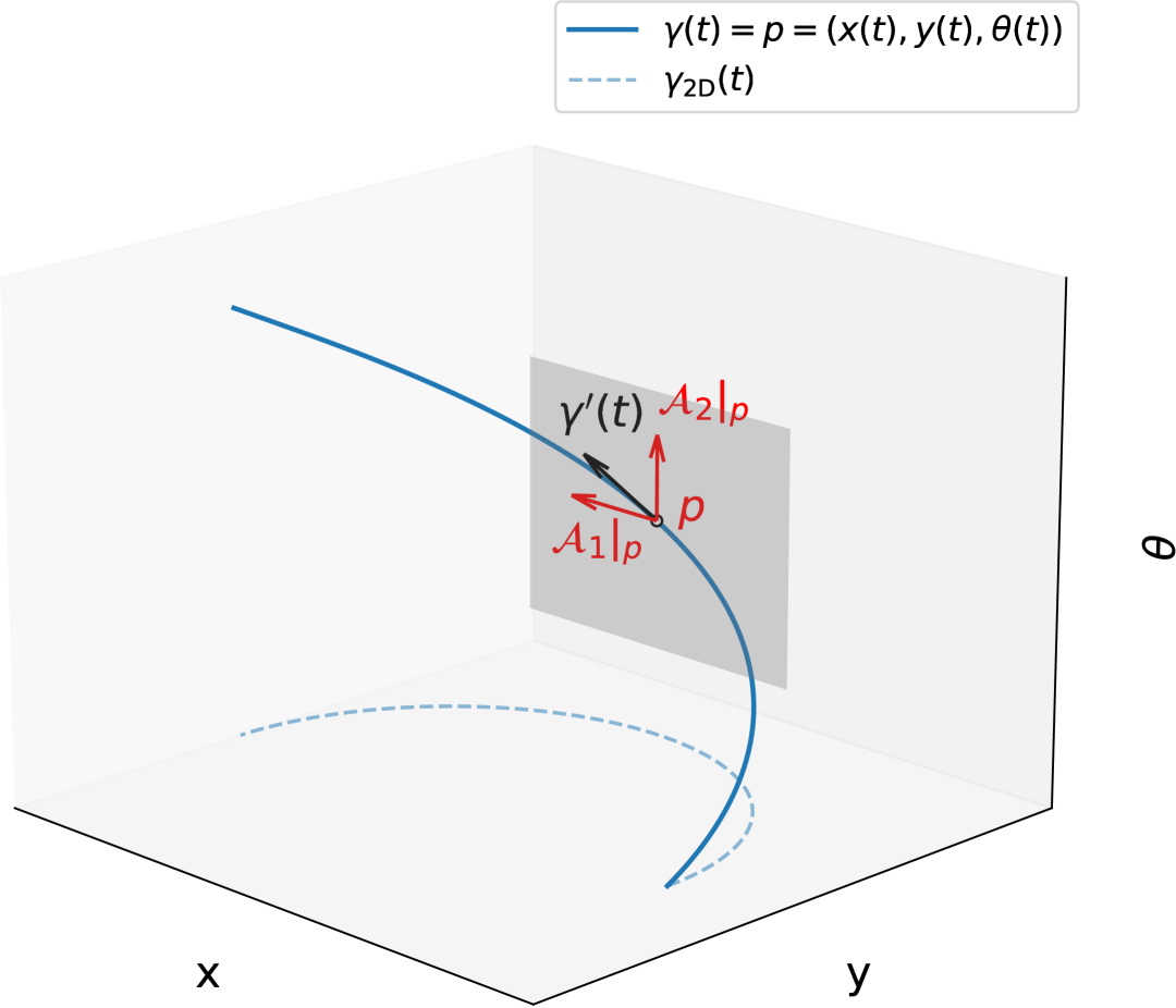
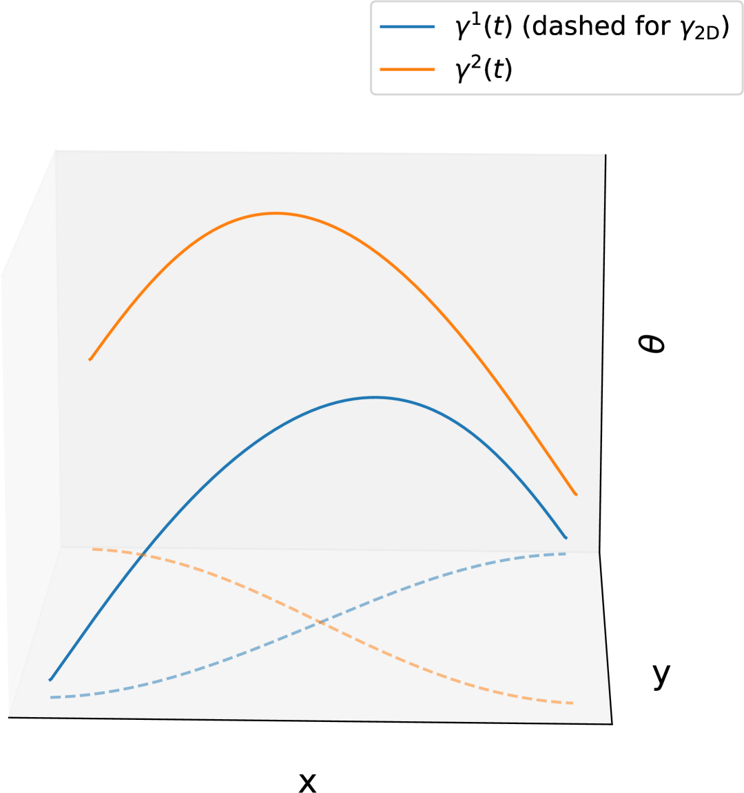
Figure 2: (Left) Each point on the planar curve $\gamma_{\text{2D}}(t)=(x(t),y(t))$ is lifted to a point $p=\gamma(t)=(x(t),y(t),\theta(t))\in\mathbb{M}_{2}$ along a horizontal curve (solid line), where $\theta(t)$ denotes the direction of the tangent vector $\dot{\gamma}_{2D}(t)$ of the original planar curve. The differential structure enables a tangent plane at $p$ spanned by $\mathcal{A}_{1}|_{p}$ and $\mathcal{A}_{2}|_{p}$, where the tangent vector $\gamma^{\prime}(t)$ lies. Adapted from [4]. (Right) The two dashed planar curves crossing in 2D are untangled in the lifting space.

1.1 Contributions

Our main contributions in this article are listed below.

• Introduce a lift of the curve recovery problem in the roto-translation space, also understood as the position-orientation space;

• Define a new regularisation on this space thanks to a Riemannian metric tailored for dynamic Dirac measure recovery, in particular for crossing trajectories;

• Prove the $\Gamma\text{-convergence}$ of the discretised curve problem to the global one, thus showing the interest of discretising the space of curves using polygonal, Bézier and piecewise geodesic curves as approximations in the practical context;

• Propose an efficient greedy algorithm, with several numerical examples to illustrate the capabilities of our proposed method. We study balanced and unbalanced cases, with polygonal, Bézier and piecewise geodesic discretisations.

1.2 Paper outline

This paper is organised as follows: the first section introduces the subject with as little mathematics and jargon as possible and gives an idea of what has been done and what elements we bring to the literature, the second section introduces the variational problem, then the third section gives theoretical insights as to why the proposed discretisations work. Finally, the last section shows our attempts to bring our method to concrete applications, with convincing results.

1.3 Notations

Let $d\in\mathbb{N}^{*}$ be the dimension of the ambient space, namely the space where the sources positions live. In the following, $\mathcal{X}$ is a closed, bounded and convex subset of $\mathbb{R}^{d}$. ${\mathscr{H}}$ is a Hilbert space, endowed with its canonical norm $\norm{\cdot}_{\mathscr{H}}$. $\mathbb{S}^{d}$ is the $d$-sphere, understood as the space of orientation. The roto-translation space will be further denoted $\mathbb{M}^{d}\stackrel{{\scriptstyle\mathrm{def.}}}{{=}}\mathbb{R}^{d}\rtimes\mathbb{S}^{d}$, for $\rtimes$ the semi-direct product pertaining to the group structure and $\operatorname{\mathrm{SO}}(d)$ the $d$-space of rotation. We also note $\wedge$ the cross-product, and $\cdot$ the dot product. Let $(X_{1},S_{1})$ and $(X_{2},S_{2})$ be two measurable spaces, $m$ be a measure on $S_{1}$ and $f:X_{1}\to X_{2}$ a measurable function. The push forward of $\mu$ is defined as the measure $f_{\sharp}\mu$ defined for all $B\in S_{2}$ by $f_{\sharp}\mu(B)\stackrel{{\scriptstyle\mathrm{def.}}}{{=}}\mu(f^{-1}(B))$. The tensor notation, and especially the Einstein notation will be used: consider $(x^{1},\dots,x^{N})$ some contravariant tensor, and a covariant tensor $(c_{1},\dots,c_{N})$ then the sum $y=\sum_{i=1}^{N}c_{i}x^{i}$ is abbreviated $y=c_{i}x^{i}$ where we omit the summation symbol.

2 Dynamic off-the-grid 101: a quick explanation on the setting

This work belongs to the calculus of variations field, with proposed applications to inverse problem: an inverse problem aims to recover some physical quantities, from a low-passed noisy observation. This is typically the localisation of sources, from a blurred, downgraded image or measurement. The off-the-grid variational methods, also called gridless methods, are a rather recent addition to the literature [12, 20, 24, 21], designed to overcome the limitations of the discrete methods, more precisely by the fine grid. Indeed, in the discrete framework such as the Basis Pursuit/LASSO, a fine grid is introduced and the sources are estimated within this setting: the point (also called spikes) are thereby constrained on this grid, further yielding discretisation discrepancies. On the contrary, off-the-grid methods do not rely on such grid and rather consist in the optimisation of a measure in terms of amplitude, position and number of the point sources, it can then fully leverage the physical knowledge of the structures we aim to retrieve. Moreover, they offer several theoretical results, such as a quantitative bound characterising the discrepancies between the source and the reconstruction. In the following, we propose a quick recall of these notions; we advise the interested reader to take a glance at the seminal papers cited before, or at [32] to get a broader vision of the domain and its applications.

2.1 Off-the-grid recovery of point sources in a static manner

The machinery behind the off-the-grid framework really boils down to the notion of measure. Several measure spaces and regularisations were proposed in the literature [12, 19, 33, 9] for distinct geometry of the sources such as points, sets, curves, etc. In the following, we will investigate for the sake of pedagogy the classic case study in the gridless methods: the recovery of point sources from one observation, without any notion of time. As defined in the notations section, let $\mathcal{X}$ be a closed, bounded and convex set of $\mathbb{R}^{d}$.

2.1.1 Radon measure space

A spike, or a point source, can physically take any position on the continuum $\mathcal{X}$; it cannot be constrained to a finite set of positions – at least in the physical world. It can be accurately modelled by a Dirac measure/masse $a\delta_{x}$: loosely speaking, this map allows us to encode both amplitude $a\in\mathbb{R}$ and spatial continuous information $x\in\mathcal{X}$ in the same object. However, since the Dirac measure is not a classic continuous function, one needs to consider a more general set of mapping called the Radon measures.

From a distributional standpoint, it is a subset of the distribution space $\mathscr{D}^{\prime}(\mathcal{X})$; the latter being the space of linear forms over the space of test functions $\mathscr{C}_{c}^{\infty}(\mathcal{X})$ i.e. smooth functions (continuous derivatives of all orders) compactly supported. In fact, it is the smallest Banach space that contains the Dirac masses. This functional approach is based on the definition of a measure as a linear form on a function space, hence we will need:

Definition 2.1 (Continuous function on $\mathcal{X}$).

We call $\mathscr{C}\left(\mathcal{X},Y\right)$ the set of continuous functions from $\mathcal{X}$ to a normed vector space $\mathcal{Y}$, endowed with the supremum norm $\norm{\cdot}_{\infty,\mathcal{X}}$ of functions.

Definition 2.2 (Evanescent continuous function on $\mathcal{X}$).

We call $\mathscr{C}_{0}\left(\mathcal{X},Y\right)$ the set of evanescent continuous functions from $\mathcal{X}$ to a normed vector space $\mathcal{Y}$, namely all the continuous map $\psi:\mathcal{X}\to\mathcal{Y}$ such that :

$$\forall\varepsilon>0,\exists K\subset\mathcal{X}\,\mathrm{compact},\quad\sup_{x\in\mathcal{X}\setminus K}\norm{\psi(x)}_{\mathcal{Y}}\leq\varepsilon.$$

We write $\mathscr{C}_{0}\left(\mathcal{X}\right)$ when $\mathcal{Y}=\mathbb{R}$. Then,

Definition 2.3 (Set of Radon measures).

We denote by ${\mathcal{M}\left(\mathcal{X}\right)}$ the set of real signed Radon measures on $\mathcal{X}$ of finite masses. It is the topological dual of $\mathscr{C}_{0}\left(\mathcal{X}\right)$ with supremum norm $\norm{\cdot}_{\infty,\mathcal{X}}$ by the Riesz-Markov representation theorem [27]. Thus, a Radon measure $m\in{\mathcal{M}\left(\mathcal{X}\right)}$ is a continuous linear form on functions $f\in\mathscr{C}_{0}\left(\mathcal{X}\right)$, with the duality bracket denoted by $\braket{f,m}_{\mathcal{M}}=\int_{\mathcal{X}}f\,\mathrm{d}m$.

A signed measure means that the quantity $\braket{f,m}_{\mathcal{M}}$ is allowed to be negative, further generalising the notion of probability, hence positive, measure. Classic examples of Radon measures are the Lebesgue measure, the Dirac measure $\delta_{z}$ centred in $z\in\mathcal{X}$ namely for all $f\in\mathscr{C}_{0}\left(\mathcal{X}\right)$ one has $\braket{f,\delta_{z}}_{\mathcal{M}}=f(z)$, etc.

The Banach space ${\mathcal{M}\left(\mathcal{X}\right)}$ can be endowed with the topology of the norm, or with the topology of its dual called the weak-$\ast$ topology.

Definition 2.4 (Weak-$\ast$ convergence).

A sequence of measures $(m)_{n\in\mathbb{N}}$ weakly-$\ast$ converges to $m\in{\mathcal{M}\left(\mathcal{X}\right)}$, denoted by $m_{n}\stackrel{{\scriptstyle\ast}}{{\rightharpoonup}}m$, if:

$$\forall g\in\mathscr{C}_{c}^{\infty}(\mathcal{X}),\quad\int_{\mathcal{X}}g\,\mathrm{d}m_{n}\xrightarrow[n\to+\infty]{}\int_{\mathcal{X}}g\,\mathrm{d}m.$$

2.1.2 Observation model

Let us introduce ${\mathscr{H}}$ the Hilbert space where the acquired data, or observation, live. In the case of images, we use a finite-dimensional space of acquisition ${\mathscr{H}}={\mathscr{H}}_{n}\stackrel{{\scriptstyle\mathrm{def.}}}{{=}}\mathbb{R}^{n}$ for $n\in\mathbb{N}$. Let $m\in{\mathcal{M}\left(\mathcal{X}\right)}$ be a source measure, we call acquisition, or observation, $y\in{\mathscr{H}}$ the result of the forward/acquisition map $\Phi:{\mathcal{M}\left(\mathcal{X}\right)}\to{\mathscr{H}}$ evaluated on $m$, with measurement kernel $\varphi:\mathcal{X}\to{\mathscr{H}}$ continuous and bounded [22]:

(1) $$y\stackrel{{\scriptstyle\mathrm{def.}}}{{=}}\Phi m=\int_{\mathcal{X}}\varphi(x)\,\mathrm{d}m(x).$$

Also note that the forward operator $\Phi$ incorporates a sampling operation, hence ${\mathscr{H}}={\mathscr{H}}_{n}$. In the following, we impose $\varphi\in\mathscr{C}^{2}(\mathcal{X},{\mathscr{H}})$ and $\forall q\in{\mathscr{H}}$, the map $x\mapsto\braket{\varphi(x),q}_{{\mathscr{H}}}$ ought to belong to $\mathscr{C}_{0}\left(\mathcal{X}\right)$. Let us also define the adjoint operator of $\Phi:{\mathcal{M}\left(\mathcal{X}\right)}\to{\mathscr{H}}$ in the weak-$\ast$ topology, namely the map $\Phi^{\ast}:{\mathscr{H}}\to\mathscr{C}_{0}\left(\mathcal{X}\right)$, defined for all $x\in\mathcal{X}$ and $p\in{\mathscr{H}}$ by $\Phi^{\ast}(p)(x)=\braket{p,\varphi(x)}_{{\mathscr{H}}}$. The choice of $\varphi$ and ${\mathscr{H}}$ is dictated by the physical acquisition process [32], with generic measurement kernels such as convolution, Fourier, Laplace, etc.

2.1.3 An off-the-grid functional: the BLASSO

Consider the source measure $m_{a_{0},x_{0}}\stackrel{{\scriptstyle\mathrm{def.}}}{{=}}\sum_{i=1}^{N}a_{0,i}\delta_{x_{0,i}}$ with amplitudes $\mathbf{a_{0}}\in\mathbb{R}^{N}$ and positions $\mathbf{x_{0}}\in\mathcal{X}^{N}$, the sparse spike problem aims to recover this measure from the acquisition $y\stackrel{{\scriptstyle\mathrm{def.}}}{{=}}\Phi m_{a_{0},x_{0}}+w$ where $w\in{\mathscr{H}}$ is an additive noise. In order to tackle this inverse problem, let us introduce the following convex functional called BLASSO [12, 20], standing for Beurling-LASSO:

($$\mathcal{P}_{\lambda}(y) \operatorname*{argmin}_{m\in{\mathcal{M}\left(\mathcal{X}\right)}}T_{\lambda}(m)\stackrel{{\scriptstyle\mathrm{def.}}}{{=}}\dfrac{1}{2}\norm{y-\Phi(m)}^{2}_{\mathcal{H}}+\lambda\absolutevalue{m}(\mathcal{X}),$$)

where $\lambda>0$ is the regularisation parameter accounting for the trade-off between fidelity and sparsity of the reconstruction. Then thanks to convex analysis results, one can establish the existence of solutions to ($\mathcal{P}_{\lambda}(y)$) as proved in [12]. The difficulties also lie in the question of uniqueness of the solution and correct support recovery: these questions were addressed in several papers in the literature [24, 21].

A very general result in the calculus of variations community called the representer theorem has been thoroughly applied to numerous off-the-grid energies, such as the BLASSO. Let $G:{\mathscr{H}}_{n}\to\mathbb{R}$ an arbitrary data fitting term; suppose that $\Lambda:\Omega\to{\mathscr{H}}_{n}$ is linear and $F:\Omega\to\mathbb{R}$ is convex, and for $m\in\Omega$ the energy reading $J(m)\stackrel{{\scriptstyle\mathrm{def.}}}{{=}}G(\Lambda m)+F(m)$. An extreme point of a convex set $S$ is a point $x\in S$ that cannot be expressed as a convex combination of two distinct points in $S$, we denote by $\operatorname{Ext}(S)$ the set of extreme points of $S$. The following theorem, due to [5, 7], establishes (up to some hypotheses) the link between the minimisers of the functional $J$ and the extreme points of the unit ball ${\mathcal{B}}_{1}^{F}\stackrel{{\scriptstyle\mathrm{def.}}}{{=}}\{u\in\Omega,F(u)\leq 1\}$:

Theorem 2.5 (Representer theorem).

If $F$ is semi-norm, there exists $\bar{u}\in\Omega$, a minimiser of $J$ with the representation:

$$\bar{u}=\sum_{i=1}^{p}\alpha_{i}u_{i}$$

where $p\leq\dim{\mathscr{H}}_{n}$, $u_{i}\in\operatorname{Ext}({\mathcal{B}}_{1}^{F})$ and $\alpha_{i}>0$ with $\sum_{i=1}^{p}\alpha_{i}=F(\bar{u})$.

This result is significant because it connects the geometry of minimisers to the structure of the regulariser $R$, and more precisely, to the extreme points of its unit ball ${\mathcal{B}}_{1}^{F}$ (or sublevel sets). Well-known examples include $\ell_{1}$ regularisation, so the BLASSO energy, whose extreme points are Dirac measures. More recently, a regulariser for divergence vector field/solenoid has also been proposed that promotes curve-like structures [33], albeit within a static framework. Leveraging the representer theorem is a thriving approach, which amounts to characterising the structural properties of minimisers without the need to explicitly solve the optimisation problem [5]. Moreover, understanding the extreme points of the unit ball of the regulariser is crucial for numerical implementation; in particular, the Frank–Wolfe algorithm reconstructs a solution by iteratively adding extreme points of the $R$-unit ball to the current estimate.

Now, we need to expand the BLASSO framework to the dynamic setting, to incorporate some dependence in time. In the latter, the observation is a stack of images, hence a sequence of images ordered by time: thereby, the point sources should be dynamic and further carry out a time dependence.

2.2 Dynamic off-the-grid point sources setting

2.2.1 The time cone framework and the push-forward measure from $\mathcal{M}(\Gamma)$ to $\mathcal{M}(\Omega)$

In the seminal papers [10, 9, 11] on off-the-grid dynamic methods, the time-cone $\Omega\stackrel{{\scriptstyle\mathrm{def.}}}{{=}}[0,1]\times\mathcal{X}$ is introduced as a natural framework for representing time-dependent sparse measures. The goal of the reconstruction is to recover multiple points that evolves over time, which can be modelled as a measure $\rho\in\mathcal{M}(\Omega)$, where $\rho(t,x)$ represents the spatial distribution of the measure at time $t$. This formulation allows the problem to be expressed as a variational optimisation problem, where one seeks to minimise a cost functional involving data fidelity and regularisation. To ensure temporal smoothness, the measure $\rho(t,x)$ is required to satisfy a continuity equation of the form $\partialderivative{t}\rho+\nabla\cdot(\rho v)=0$, where $v$ is a velocity field governing the transport of mass. While $\mathcal{M}(\Omega)$ provides a useful representation of time-dependent measures, it does not explicitly encode trajectories of moving sources. To better capture the underlying dynamical structure, the problem is reformulated in terms of measures on paths, transitioning from $\mathcal{M}(\Omega)$ to $\mathcal{M}(\Gamma)$, where $\mathcal{M}(\Gamma)$ represents distributions over smooth particle trajectories $\Gamma$.

This reformulation allows each point source to be described by a continuous path $\gamma=(h,\xi)$, where $h(t)$ denotes its mass and $\xi(t)$ its trajectory over time $t$. By leveraging this representation, the problem inherently enforces smooth motion constraints and naturally integrates optimal transport regularisation. This transformation is justified by measure disintegration techniques, enabling one to decompose the measure as a product separating time and spatial components. Moreover, it establishes a one-to-one correspondence between the solutions of the continuity equation in $\mathcal{M}(\Omega)$ and measures on $\mathcal{M}(\Gamma)$. From a computational perspective, this approach enables off-the-grid optimization methods, avoiding the need for space-time discretisation while facilitating efficient implementation through graph-based shortest-path algorithms [25].

Thus, working in $\mathcal{M}(\Gamma)$ leads to a more structured and computationally tractable formulation of dynamic inverse problems. In the following section, we give a precision definition of these spaces and Benamou-Brenier regularisation, ensuring that the reconstructed point sources follow smooth trajectories over time. Consequently, since each spike is detected based on the discretised observation, this penalty reduces the set of possible paths to only those that are smooth and physically meaningful.

2.3 An energy for trajectories recovery

Let $T\in\mathbb{N}^{*}$ be the number of time samples, further defining $(t_{i})_{1\leq i\leq T}$ the time slices ranging from 0 to 1: $0\leq t_{i}\leq 1$, and ${\mathscr{H}}$ is an Hilbert space. The following functional is the core component of the dynamic off-the-grid framework [9, 11] so far:

(2) $$\operatorname*{argmin}_{\sigma\in\mathcal{M}(\Gamma)}E(\sigma)=\operatorname*{argmin}_{\sigma\in\mathcal{M}(\Gamma)}\sum_{i=1}^{T}\norm{A_{i}e_{t_{i}\sharp}\sigma-b_{t_{i}}}_{\mathscr{H}}+\int_{\Gamma}w(\gamma)\,\mathrm{d}\sigma(\gamma),$$

We ought to precise some of the quantities introduced here:

• $t\mapsto b_{t}\in{\mathscr{H}}$ are the acquired data called the observation,

• $\Gamma=\left\{\gamma=(h,\xi),\quad h\in C([0,1],\mathbb{R}),\quad\xi:[0,1]\xrightarrow{}\mathcal{X},\quad\xi_{|h\neq 0}\text{ is continuous}\right\}$ is the space of trajectories with $h$ the amplitude weighting the mass and $\xi$ the curve,

• $e_{t}$ is the measurable map of evaluation at time $t$, defined by $e_{t}(\gamma)=\gamma(t)$ hence $e_{t\sharp}\sigma\in\mathcal{M}(\Omega),$

• $A_{i}:\mathcal{M}(\Omega)\xrightarrow{}{\mathscr{H}}$ a linear operator, pertaining to the physical context (in the case of super-resolution, the Gaussian convolution for example). The $i$ index shows that the operator can incorporate some changes over time (such as the spread of the Gaussian convolution),

• $w:\Gamma\xrightarrow{}\mathbb{R}_{+}$ a weight function, usually $w(\gamma)=\int_{0}^{T}\alpha+\beta|\dot{\gamma}|^{2}(t)\,\mathrm{d}t$ for $\alpha,\beta>0$. Once integrated and for $\alpha=0$, it constitutes the Benamou-Brenier regularisation; it only caters for the balanced case, i.e. conserved mass such as $\gamma=(1,\xi)$ .

Remark 2.6.

$\mathcal{M}(\Gamma)$ is well-defined as a complete separable metric space, since $\Gamma$ is neither locally compact nor $\sigma$-compact. See [25] for more grounded arguments.

This lies into the general framework, now set ${\mathscr{H}}=\mathbb{R}^{n}$ and:

$$A_{i}:\rho\in\mathcal{M}(\Omega)\mapsto\left(\int_{\Omega}a_{i}^{j}(x)\,\mathrm{d}\rho(x)\right)_{1\leq j\leq n}\in{\mathscr{H}}.$$

Also we need to reduce ourselves to physically meaningful curves, with some continuity assumption [2, Definition 1.1.1]:

Definition 2.7 (Absolutely continuous curves).

Absolutely $p$-continuous curves in a metric space $(X,d)$ where $p\in]1,+\infty]$ are curves $\gamma:[0,1]\longrightarrow X$ such that there exists $\zeta\in L^{p}([0,1],\mathbb{R})$ and for all $s,t$ s.t. $0\leq s\leq t\leq 1$:

(3) $$d\left(\gamma(t),\gamma(s)\right)\leq\int^{t}_{s}\zeta(u)\,\mathrm{d}u.$$

The set of such curves is denoted $\mathrm{AC}^{p}([0,1],X)$, or simply $\mathrm{AC}([0,1],X)$ if $p=1$.

More properties on absolute continuous curves such as their metric derivative, equal to the metric-norm of the classical derivative, are expressed in Appendix A. It gives rigorous definitions of these concepts for the Riemannian generalisation involved in the following sections. Now, we recall the main result [9, Theorem 10] for the Benamou-Brenier regularisation.

Theorem 2.8 (Solutions of balanced recovery from).

The energy $E$ admits a minimiser $\rho^{*}$ which is a finite sum of extreme points of the Benamou-Brenier unit ball, i.e.

$$\exists a_{i}>0,\xi_{i}\in\mathrm{AC}^{2}([0,1],\mathcal{X}),\quad\forall t\in[0,1],\quad\rho^{*}(t)=\sum_{i=1}^{T}a_{i}\delta_{\xi_{i}(t)}$$

The unbalanced case, i.e. with varying amplitude, has been treated in the literature through the Wasserstein-Fisher-Rao (WFR) regularisation [8, 25]. In the following, we will introduce our Riemannian framework for the balanced case, but we stress that our ideas hold even for WFR regularisation, which is more suited to the biomedical case we strive to solve.

The seminal papers have proven the efficiency of this optimal transport based method, as it has been shown to successfully recover the paths of moving spikes. However, the numerical implementation struggles to recover crossing paths: this is an expected behaviour, as the algorithm cannot infer the correct paths from the dual certificate (see [24]). This ambiguity is inherent to the considered energy: in the following, we will explore our proposed workaround which exploits a lifting to the space of roto-translation inspired by [15, 23], while formulating a new energy with a Riemannian regularisation tailored for paths untangling.

3 Our proposed lifting: an insight in Riemannian and numerics

3.1 The orientation-position space

As we mentioned earlier, the original curve reconstruction model struggles to recover multiple crossing curves in 2D. Indeed, the regularising term in (2) selects solutions with minimal length in the 2D plane, thus preferring couples of nearly-touching curves to crossing curves. This is all the more unfortunate as this formulation does not fully address the problems encountered in the biomedical applications: as we pointed out before, the curves frequently crossed themselves on the acquisition, and the method above cannot handle well this rather frequent case. To prevent such issue, we propose an approach consisting in lifting our setting $\mathcal{X}$ in the space of position and orientation, adding an orientation coordinate to our 2D variable.

Hence, we lift the problem in a suitable space to allow the disentanglement, further inspired by the variational approach proposed by [15]. The orientation-position space, also called the roto-translation space in the Lie group literature, is understood as a homogeneous space upon which the Special Euclidean group $\operatorname{\mathrm{SE}}(d)=\mathbb{R}^{d}\rtimes\operatorname{\mathrm{SO}}(d)$ acts transitively and faithfully. $\operatorname{\mathrm{SO}}(d)$ the d-dimensional rotation group, i.e. the group of all rotations about the origin of $d$-dimensional Euclidean space $\mathbb{R}^{d}$ under the operation of composition.

As mentioned earlier, $\mathcal{X}\subset\mathbb{R}^{d}$ is then the spatial domain where the acquisition is defined, and $\mathbb{S}^{d-1}$ thereby parametrises the local orientation of the curve.

Definition 3.1.

The homogeneous space of orientation-position in $\mathbb{R}^{d}$ is:

$$\mathbb{M}_{d}\stackrel{{\scriptstyle\mathrm{def.}}}{{=}}\mathbb{R}^{d}\times\mathbb{S}^{d-1}.$$

We fill also refer to it as the roto-translation space.

Remark 3.2.

The semidirect product, denoted by $\rtimes$, fundamentally differs from the direct product ($\times$) in that it allows for a non-commutative interaction between its constituent groups. Unlike a direct product where elements from one subgroup commute with elements from the other, in a semidirect product, one subgroup acts on the other. Consequently, the composition of elements, such as two roto-translations, is generally order-dependent. Stricly speaking, $\mathbb{M}_{d}\stackrel{{\scriptstyle\mathrm{def.}}}{{=}}\mathbb{R}^{d}\rtimes\mathbb{S}^{d-1}$ but since we do not compose elements of $\mathbb{M}_{d}$, choosing the semidirect product or the direct product here makes no substantial difference.

It is a $(2d-1)\text{-dimensional}$ manifold, in the following we will consider examples in $d=2$ since our biomedical application is set on 2–dimensional images and we feel that this case is more pedagogical: however, note that our solution still applies to any $n$D setting. The space $\mathbb{M}_{2}$ is useful because it allows one to differentiate objects with the same position but with different orientations, which is a common feature in $2D$ vessel images, as the projection in a $2D$ image of a tree-like structure gives rise to crossings.

If needed and for computational ease, we will identify $n=(\cos(\theta),\sin(\theta))\in\mathbb{S}^{1}\longleftrightarrow\theta\in\mathbb{R}/\mathbb{Z}\longleftrightarrow R_{\theta}\in\operatorname{\mathrm{SO}}(2)$, since $\mathbb{S}^{1}$ is isomorphic to $\operatorname{\mathrm{SO}}(2)$. As of now, $N\in\mathbb{N}^{*}$ control points will no longer belong to $\mathcal{X}^{N}$ but rather in the manifold $\left(\mathbb{M}_{d}\right)^{N}$ to further incorporate orientation information in the curve. The roto-translational curve space is then:

$$\Upsilon\stackrel{{\scriptstyle\mathrm{def.}}}{{=}}\left\{\gamma=(h,\xi),\quad h\in C([0,1],\mathbb{R}),\quad\xi:[0,1]\xrightarrow{}\mathbb{M}_{d},\quad\xi_{|h\neq 0}\text{ is continuous}\right\}$$

and the measure space $\mathcal{M}(\Upsilon)$ follows naturally. Eventually, note that the original roto-translational space $\mathbb{M}_{d}$ is a Riemannian manifold, hence a vector space with more structure thanks to the metric tensor. This Riemannian structure will be leveraged to further implement the regularisation on curves crossing, see Figure 2, but beforehand it calls for a quick introduction.

3.2 A relaxed metric on the orientation-position space

We ought to begin this section with a recall on differential geometry, in particular for Riemannian or flavour-liked manifold, as we strive to make this paper self-contained. Note that not only these notions are mandatory to define our metric/regularisation, but they are also needed to perform the numerical implementation through Riemannian optimisation. Be careful as in this section, $\gamma$ denotes a geodesic and not the couple $(h,\xi)\in\Gamma$ of amplitude and path.

3.2.1 Riemannian geometry basics

As in 1946, Élie Cartan stated that ’the general notion of manifold is quite difficult to define precisely’ [13]; in this vein the notions exhibited below will be defined rather informally, as we think the reader should focus more on the underlying idea than the formal setting. However, we strongly advise the interested reader, willing to learn more about Riemannian geometry, to take a glance at [34, 1, 29, 40] for a rather more far-reaching presentation.

Let $\mathcal{M}$ be a smooth $d$-manifold, namely a space where one can lay down everywhere local coordinates $(x^{1},\dots,x^{d})$ i.e. homeomorphism mapping open set of $\mathcal{M}$ to an open set of $\mathbb{R}^{d}$. It is a generalisation of the notion of smooth surface of $\mathbb{R}^{d}$, that one can bend, twist, and curve smoothly in any direction without any creases or sharp corners; bar the manifold does not rely on the ambient space for its definition. A smooth manifold is then a space that locally resembles a Euclidean space. On each point $p\in\mathcal{M}$ one can define the tangent space $\mathcal{T}_{p}\mathcal{M}$: it can be seen as a linearisation of the manifold at $p$. A tangent space is a vector space, enjoying an ordered basis. The union of all point of the manifold and their associated tangent space is called the tangent bundle $\mathcal{T}\mathcal{M}\stackrel{{\scriptstyle\mathrm{def.}}}{{=}}\left\{(p,v)\,|\,p\in\mathcal{M},v\in\mathcal{T}_{p}\mathcal{M}\right\}$.

The manifold can be equipped with a metric $g$ i.e. a symmetric covariant tensor field, also denoted $g_{ij}$ in tensor notation, defined on the tangent bundle. The restriction at $p\in\mathcal{M}$ is denoted by $g_{p}:\mathcal{T}_{p}\mathcal{M}\times\mathcal{T}_{p}\mathcal{M}\to\mathbb{R}$, it is an inner product that maps two vectors lying on the tangent space of $p$ onto a real number. Loosely speaking, a Riemannian manifold $(M,g)$ is a smooth manifold with a smoothly varying inner product $g_{p}$ on the associated tangent spaces. We further denote $\norm{\cdot}_{g}\stackrel{{\scriptstyle\mathrm{def.}}}{{=}}\sqrt{g(\cdot,\cdot)}$ the metric norm.

The metric admits a contravariant inverse tensor reading $g^{-1}$, or $g^{ij}$. It is uniquely defined by $\delta^{i}_{k}=g_{jk}g^{ij}$ where $\delta_{ij}$ is the Kronecker symbol. A core component of Riemannian geometry is the geodesic, the generalisation in the Riemannian manifold $(\mathcal{M},g)$ context of straight lines of the Euclidean setting.

Definition 3.3 (Geodesic).

In the sense of the calculus of variations, a geodesic is a continuously differentiable $\gamma:[0,1]\to\mathcal{M}$ such that it is a minimum of the energy:

(4) $$E_{\mathrm{c}}(\gamma)\stackrel{{\scriptstyle\mathrm{def.}}}{{=}}\dfrac{1}{2}\int_{0}^{1}g_{\gamma(t)}\left(\gamma^{\prime}(t),\gamma^{\prime}(t)\right)\,\mathrm{d}t.$$

A geodesic can be thought of as a free particle $\gamma(t)$ such that its acceleration has no component in the direction of the surface, hence at each point $p=\gamma(t)$ of the curve it is perpendicular to the tangent plane $\mathcal{T}_{p}\mathcal{M}$ of the manifold.

A Riemannian manifold can then be endowed with the geodesic metric, then

(5) $$\forall(p,q)\in\mathcal{M}^{2},\quad{d_{g}}(p,q)\stackrel{{\scriptstyle\mathrm{def.}}}{{=}}\inf_{\begin{subarray}{c}\gamma\in\mathrm{AC}([0,1],X)\\ \gamma(0)=p,\gamma(1)=q\end{subarray}}\int_{0}^{1}\norm{\gamma(t)}_{g}^{2}\,\mathrm{d}t.$$

Consider a smooth map on the manifold $f:\mathcal{M}\to\mathbb{R}$, its Riemannian gradient at $x$ lies in the tangent space $\mathrm{grad}f\in\mathcal{T}_{x}\mathcal{M}$. For $\mathcal{M}\subset\mathbb{R}^{d}$, it is related to the Euclidean gradient $\operatorname{grad}_{\mathbb{R}}f:\mathbb{R}^{d}\to\mathbb{R}$, the classical gradient defined in the ambient space, by:

$$\operatorname{grad}f=g^{-1}\operatorname{grad}_{\mathbb{R}}f,\quad\mbox{also written }\operatorname{grad}f_{i}=g^{ij}\operatorname{grad}_{\mathbb{R}}f_{j}.$$

Obviously, a vector $v$ of the tangent plane $\mathcal{T}_{x}\mathcal{M}$ has no reason to belong to the manifold, and an iterate of the gradient descent might then escape the manifold. A tool from the differential geometry can then be leveraged:

Definition 3.4 (Exponential map).

Let $v\in\mathcal{T}_{p}\mathcal{M}$ a tangent vector of the manifold at point $p$. Then, there exists a unique geodesic $\gamma_{v}:[0,1]\to\mathcal{M}$ such that $\gamma(0)=p$ and $\gamma^{\prime}_{v}(0)=v$. The exponential map is defined by:

$$\operatorname{\mathrm{Exp}}_{p}(v)=\gamma_{v}(1).$$

The application $\operatorname{\mathrm{Exp}}_{p}$ acts as a local diffeomorphism from the tangent space $T_{p}\mathcal{M}$ to $\mathcal{M}$. When defined, its inverse $\operatorname{\mathrm{Log}}_{p}:\mathcal{M}\to\mathcal{T}_{p}M$ is called the logarithmic map.

The optimisation in the Riemannian setting is a powerful tool leveraging the structure offered by the manifold: as the solution must lie in $M$, each iteration remaps the new iterate onto the manifold with the exponential map. In contrast, Euclidean optimisation may escape the manifold and might struggle to converge to the solution, getting trapped into local minima outside the set, in the ambient space (if defined).

In Riemannian geometry and in particular for optimisation, we may need to move a vector defined on a tangent space $\mathcal{T}_{x}\mathcal{M}$ to another tangent space $\mathcal{T}_{y}\mathcal{M}$. The new tangent space $\mathcal{T}_{y}\mathcal{M}$ enjoys an ordered basis, differing from those of $\mathcal{T}_{x}\mathcal{M}$: these changes in the two coordinate systems are encapsulated in the Christoffel symbols $\Gamma^{k}_{ij}$: it accounts for the change in the $i$-th component caused by a change of the $j$-th component, computed in the $k$-th component direction. Christoffel symbols completely define the metric tensor, and conversely; it also comes handy for second order Riemannian optimisation scheme . Moreover, it is useful for geodesics computation as it appears in this fundamental ordinary equation:

Theorem 3.5 (Geodesic equation).

Given initial conditions $p\in\mathcal{M}$, $v\in\mathcal{T}_{p}\mathcal{M}$, a geodesic $\gamma:[0,1]\to\mathcal{M}$ is a solution of:

(6) $$\derivative[2]{\gamma^{k}}{t}+\Gamma_{ij}^{k}\derivative{\gamma^{i}}{t}\derivative{\gamma^{j}}{t}=0,$$

with $\gamma(0)=p$ and $\gamma^{\prime}(0)=v$. This is simply the Euler-Lagrange equations of the action in equation (4), expressed in local coordinates: $\gamma^{i}\stackrel{{\scriptstyle\mathrm{def.}}}{{=}}x^{i}\circ\gamma(t)$.

Eventually, for the optimisation in a Riemannian setting, we advise the reader to look up the Appendix D.

These notions are rather general but compulsory as we work with the $\mathbb{M}^{d}$ manifold, hence we need to perform a optimisation exploiting the underlying Riemannian structure. We can now leverage this knowledge with our proposed lift on the rototranslation space $\mathbb{M}_{d}$.

3.2.2 The Reeds-Shepp metric

Multiple models have taken advantage of the space of roto-translation $\mathbb{M}_{d}$, among which applications we could quote computing geodesics taking into account orientation features and penalising curvature. Usually used to model vehicles with forward and reverse gears or oriented objects in $\mathbb{R}^{d},$ the Reeds-Shepp metric [37] has numerous applications in various context. It is a sub-Riemannian metric that prevents curves from being planar and penalises changes of direction (meaning penalising curvature of the trajectory). We will use a relaxed Riemannian version $\mathcal{F}_{\varepsilon}$ of the Reeds-Shepp metric $\mathcal{F}$ here that only penalises velocities orthogonal to. This model continuously converges to the standard sub-Riemannian Reeds-Shepp metric [23] as the relaxation parameter $\varepsilon$ yields $0$.

There is several examples of the roto-translational space and Reeds-Shepp metric in medical images processing, such as in [3] which applies filters on lifted images to help track blood vessels in vascular imaging and in [4] for the computation of geodesics in $\operatorname{\mathrm{SE}}(2)$. The following definition of $\mathcal{F}_{\varepsilon}$ is peculiar to the biomedical application.

Definition 3.6 (Relaxed Reeds-Shepp metric).

The relaxed Reeds-Shepp metric tensor field $g$ [23] can be written as a Euclidean norm at each point in $\mathbb{M}_{2}$. Let $0<\varepsilon\leq 1$ be the relaxation parameter, $\xi>0$ a scaling parameter, consider $(x,\theta)\in\mathbb{M}_{2}$ while $(\dot{x},\dot{\theta})\in\mathcal{T}_{(x,\theta)}\mathbb{M}_{2}$ lies in the tangent plane, then:

$$g_{(x,\theta)}\left((\dot{x},\dot{\theta}),(\dot{x},\dot{\theta})\right) \stackrel{{\scriptstyle\mathrm{def.}}}{{=}}|\dot{x}\cdot e_{\theta}|^{2}+\frac{1}{\varepsilon^{2}}|\dot{x}\wedge e_{\theta}|^{2}+\xi^{2}|\dot{\theta}|^{2}$$

$$=\left<R_{\theta}(\dot{x},\dot{\theta}),\mathrm{diag}\left(1,\frac{1}{\varepsilon^{2}},\xi^{2}\right)R_{\theta}(\dot{x},\dot{\theta})\right>_{\operatorname{\mathrm{SO}}(2)},$$

where $e_{\theta}$ is the unit vector in the direction defined by the angle $\theta$, $R_{\theta}$ is the rotation matrix and the bracket is the classical Euclidean inner product.

The idea of this relaxation boils down to the increasing penalisation of non-planarity of the lifted path as $\varepsilon$ nears $0$. The relaxed version of Reeds-Shepp accurately approaches the sub-Riemannian case with infinite cost for non-planar curves. The $\absolutevalue{\dot{\theta}}^{2}$ term penalises steering the prescribed orientation of the curve, and acts as a penalisation of the local curvature of the curve. As we have defined a regularisation function embodied in the Reeds-Shepp metric, the problem is further written down as the optimisation of the following energy:

(7) $$\operatorname*{argmin}_{\sigma\in\mathcal{M}(\Upsilon)}T_{\beta,\varepsilon}(\sigma)=\operatorname*{argmin}_{\sigma\in\mathcal{M}(\Upsilon)}\sum_{i=1}^{T}\norm{A_{i}e_{t_{i}\sharp}\sigma-b_{t_{i}}}_{\mathscr{H}}+\beta\int_{\Gamma}\int_{0}^{1}\norm{\gamma^{\prime}(t)}_{g}\,\mathrm{d}t\,\mathrm{d}\sigma(\gamma).$$

Theoretical guarantees proven by the original authors still hold, see appendix B for a more rigorous proof that the paths extreme points are conserved with this energy (7). Before illustrating our proposed energy on some numerical examples, one can genuinely raise some concern on the theoretical soundness of discretising the measure problem, as in practice the UFW presented in section 5 recovers discretised curves, since the computers cannot embed a computation with infinite precision. Do we need an infinity of control points to correctly describe the solution of the variational problem? In the following, we try to fully address this issue by considering multiple discretisations of curve and by proving $\Gamma$-convergence results.

4 $\Gamma$-convergence of several discretisation in the Benamou-Brenier case

This section is motivated by numerical soundness, but also covers a point raised by [25, Lemma 3.3]. Indeed, for

$$W:\gamma\mapsto\tilde{\gamma}\in\operatorname*{argmin}\left\{w(\chi)\,|\,\chi\in\Gamma,0\leq i\leq T,\chi(t_{i})=\gamma(t_{i})\right\}$$

one has $E\left(W_{\sharp}\gamma\right)\leq E(\gamma)$, with $w(\gamma)=\alpha+\beta\int_{0}^{1}\norm{\gamma^{\prime}(t)}_{g}^{2}\,\mathrm{d}t$. This implies the existence of a theoretically optimal discretisation of the space: any candidate solution to the optimisation problem can be replaced by a better one, as long as it preserves the position of the curve at the timestamps where the data term is evaluated. In other words, the optimal curves are piecewise ’geodesic’ with respect to the weight function $w$ between each pair of timestamps $t_{i}$.

We now turn to discretising the space of curves to obtain a good approximation of the solution to problem (2), and a fortiori the energy in equation (7) with the Reeds-Shepp metric. In this section, we present a formulation for approximating absolutely continuous curves using families of curves defined by a finite number of control points. Note that these results are expressed for any $\mathcal{X}\subset\mathbb{R}^{d}$ threfore $\mathcal{M}(\Gamma)$, hence holds for submanifold $\mathbb{M}_{d}$ and associated $\mathcal{M}(\Upsilon)$. We then consider a generic $\Gamma$ with its metric tensor $g$ (e.g. Reeds-Shepp).

4.1 A suitable definition for convergence

We need to qualify the convergence of the surrogate problems to the continuous one. For this point, we will rely on the following notion of functional convergence.

Definition 4.1 ($\Gamma$-convergence).

Let $X$ a first countable space, $F_{n}:X\to\mathbb{R}$ a sequence of functionals. We say that $F_{n}$ sequence of functions $\Gamma$-converges to its $\Gamma$-limit $F:X\to\mathbb{R}$ if the two conditions hold:

• (Liminf inequality) for every sequences $x_{n}\in X$ such that $x_{n}\stackrel{{\scriptstyle\ast}}{{\rightharpoonup}}x$:

  $$F(x)\leq\liminf_{n\to\infty}F_{n}(x_{n}).$$

• (Limsup inequality) there exist a sequence $x_{n}\in X$ such that $x_{n}\stackrel{{\scriptstyle\ast}}{{\rightharpoonup}}x$ and :

  $$F(x)\geq\limsup_{n\to+\infty}F_{n}(x_{n}).$$

When defined, the limit is denoted $\Gamma\mathrm{-lim}_{n\to+\infty}$ or more concisely $\Gamma\mathrm{-lim}_{n}$, hence with the latter notations $F=\Gamma\mathrm{-lim}_{n}F_{n}$. The interested reader can take a deeper dive in [36, 6] to learn more. This approach is common in calculus of variations, as it allows difficult—often non-convex—problems to be approximated by simpler ones that are more tractable. Among other properties, this functional convergence ensures [6, Remark 2.11] the weak-$\ast$ convergence of the minimisers (up to subsequences) of the discretised problems $F_{n}$ towards the minimisers of the continuous one $F$.

4.2 Discretisation on the space of curves

We will now consider how to discretise the space of curves in order to find a good approximation of the solution of the problem (2). In this section, we provide a formulation for the approximation of absolutely continuous curves using families of curves defined by finite-dimensional control points.

Let $P^{n}$ be a map from the space of control points $\mathbb{R}^{d\times k_{n}}$, for $k_{n}\in\mathbb{N}$ the number of control points, and $P_{n}=P^{n}(\mathbb{R}^{d\times k_{n}})$ the $n$-th order discretisation of the space of curves. Let $\mu\in\mathcal{M}(\mathbb{R}^{d\times k_{n}}),$ then we have $P^{n}_{\sharp}\mu\in\mathcal{M}(\Gamma).$ The following result ensures that, with a few assumptions, that the sequence of approximation spaces $P_{n}$ are good approximations to find the minimisers of the energy in equation (2). Let $\chi_{P_{n}}(\gamma)=0$ if $\gamma\in P_{n}$ and $+\infty$ otherwise.

Theorem 4.2.

Let $P_{n}\subset\Gamma$ be a sequence of subsets of $\Gamma$, such that $\bigcup_{n}P_{n}$ is dense in $\Gamma.$ For every $\gamma\in\Gamma$, let there be a sequence of measurable maps $S_{n}:\gamma\in\Gamma\mapsto\mathbb{R}^{d\times k_{n}}$ such that $P^{n}(S_{n}(\gamma))\longrightarrow\gamma$ for the uniform convergence. Suppose $w(P^{n}(S_{n}(\gamma)))\leq w(\gamma).$ Then the energy $E$ in equation (2) constrained to $P_{n}$ $\Gamma$-converges to $E$, i.e. $\Gamma\text{-}\mathrm{lim}_{n}(E+\chi_{P_{n}})=E$.

Proof 4.3.

Consider a sequence $(\sigma_{n})_{n\geq 0}$ such that $\sigma_{n}\stackrel{{\scriptstyle\ast}}{{\rightharpoonup}}\sigma$ in ${\mathcal{M}\left(\Gamma\right)}$. Then, since

$$E(\sigma_{n})\leq E_{n}(\sigma_{n}),$$

by lower semi-continuity, we conclude that:

$$E(\sigma)\leq\liminf_{n\to+\infty}E_{n}(\sigma_{n}).$$

For the $\limsup$ inequality, choosing $\sigma_{n}=(P^{n}\circ S_{n})_{\sharp}\sigma\xrightharpoonup{*}\sigma$, the hypothesis yields

$$\int_{\Gamma}w(\gamma)\,\mathrm{d}\sigma_{n}\leq\int_{\Gamma}w(\gamma)\,\mathrm{d}\sigma,$$

and thus:

$$\limsup_{n\to+\infty}\int_{\Gamma}w(\gamma)\,\mathrm{d}\sigma_{n}\leq\int_{\Gamma}w(\gamma)\,\mathrm{d}\sigma.$$

By continuity, we finally yield:

$$\limsup_{n\to+\infty}E_{n}(\sigma_{n})\leq E(\sigma).$$

Remark 4.4.

We may notice that the former proof defines an approximation map on $P_{n}.$ Let $S_{n}:\gamma\mapsto S_{n}(\gamma)$ be a measurable map, then $\gamma^{n}=P^{n}(S_{n}(\gamma)),$ and we retrieve $\sigma_{n}=\left(P^{n}\circ S_{n}\right)_{\sharp}\sigma.$ If we have $S_{n}\circ P^{n}=\mathrm{Id}$ as in the case of polygonal lines, it is even a projection.

The latter result requires no more than very general hypotheses and can be extended to more general settings. For instance, we may consider the time-continuous setting [11] where the data term is changed to $\int_{0}^{1}\|Ae_{t\sharp}\sigma-b_{t}\|^{2}_{\mathscr{H}}\,\mathrm{d}t$, although we loose the application of the representer theorem [5, 7] that guarantees the shape of the minimiser. Moreover, the only hypothesis on the integrand $w(\gamma)$ relies on its lower semicontinuity, so we could now consider many different regularisers, such as the Reeds-Shepp metric used earlier. On the contrary to [31], one do not have to exhibit a discrete set of solutions to get the convergence, only the inequality for the limsup property. We can then detail some classic curve discretisation, fulfilling the hypothesis.

Definition 4.5 (Curve discretisation).

Let $c\in\Gamma^{k_{n}}$ be the control points of the discretised curve:

• Polygonal lines, $k_{n}$ s.t. $k_{n}|k_{n+1}$ ($k_{n}$ divides $k_{n+1}$) hence $P_{n}\subset P_{n+1}$, $\tilde{t}_{k}=\frac{k}{k_{n}}$,

  $$P^{n}(c)(t)=\frac{\tilde{t}_{k+1}-t}{\tilde{t}_{k+1}-\tilde{t}_{k}}c_{k}+\frac{t-\tilde{t}_{k}}{\tilde{t}_{k+1}-\tilde{t}_{k}}c_{k+1},\quad\text{if }t\in[\tilde{t}_{k},\tilde{t}_{k+1}[$$

• Bézier curves, $P^{n}(c)(t)=\sum_{k=0}^{n}t^{k}(1-t)^{n-k}\binom{n}{k}c_{k}$,

• Piecewise geodesic, for $k_{n}|k_{n+1}$, there exists $0\leq k\leq n$ such that $t\in\left[\frac{k}{n},\frac{k+1}{n}\right]$

  $$P^{n}(c)(t)=\operatorname{\mathrm{Exp}}_{c_{k}}\left(k_{n}\left(t-\frac{k}{k_{n}}\right)\operatorname{\mathrm{Log}}_{c_{k}}(c_{k+1})\right)$$

Claim 1.

The latter operators verify $w(P^{n}(S_{n}(\gamma)))\leq w(\gamma)$.

Proof 4.6.

For the sake of clarity, we exhibit the inequality for one curve $\gamma$, meaning $\sigma=\delta_{\gamma}$; the generalisation to multi-curve $\sigma=\sum_{i}\alpha_{i}\delta_{\gamma_{i}}$ is straightforward by the triangle inequality of the metric norm. Let us check that the three classical discretisations fulfill the property:

• Polygonal curves case: taking $(S_{n}(\gamma))_{k}=\gamma(\tilde{t}_{k}),$

  $$\int_{0}^{1}\left\|P^{n}(S_{n}(\gamma))^{\prime}(t)\right\|_{g}^{2}\,\mathrm{d}t$$

  $$=\int_{0}^{1}\left\|\sum_{k=0}^{k_{n}-1}\mathbbm{1}_{[\tilde{t}_{k},\tilde{t}_{k+1}]}(t)\left[\gamma(\tilde{t}_{k+1})-\gamma(\tilde{t}_{k})\right]\right\|_{g}^{2}/(\tilde{t}_{k+1}-\tilde{t}_{k})^{2}\,\mathrm{d}t$$

  $$=\sum_{k=0}^{k_{n}-1}(\tilde{t}_{k+1}-\tilde{t}_{k})\left\|\int^{\tilde{t}_{k+1}}_{\tilde{t}_{k}}\gamma^{\prime}(s)\,\mathrm{d}s\right\|_{g}^{2}/(\tilde{t}_{k+1}-\tilde{t}_{k})^{2}$$

  $$\leq\sum_{k=0}^{k_{n}-1}\int^{\tilde{t}_{k+1}}_{\tilde{t}_{k}}\left\|\gamma^{\prime}(s)\right\|_{g}^{2}\,\mathrm{d}s$$

  $$=\int^{1}_{0}\left\|\gamma^{\prime}(s)\right\|_{g}^{2}\,\mathrm{d}s.$$

• Bézier curves: taking $S_{n}(\gamma)\in\mathbb{R}^{d\times(n+1)}$, then $(S_{n}(\gamma))_{k}=\gamma(k/n),$

  $$\int_{0}^{1}\left\|P^{m}(S_{n}(\gamma))^{\prime}(t)\right\|_{g}^{2}\,\mathrm{d}t$$

  $$=\int_{0}^{1}\left\|\sum^{m-1}_{0}\binom{m-1}{k}t^{k}(1-t)^{m-1-k}(\frac{\gamma((k+1)/m)-\gamma(k/m)}{1/m})\right\|_{g}^{2}\,\mathrm{d}t$$

  $$\leq_{\text{Jensen}}\sum_{k=0}^{m-1}\binom{m-1}{k}\int_{0}^{1}t^{k}(1-t)^{m-1-k}\left\|\frac{\gamma((k+1)/m)-\gamma(k/m)}{1/m}\right\|_{g}^{2}\,\mathrm{d}t$$

  $$=\sum_{k=0}^{m-1}\binom{m-1}{k}\int_{0}^{1}t^{k}(1-t)^{m-1-k}\left\|\frac{\int_{k/m}^{(k+1)/m}\gamma^{\prime}(s)\,\mathrm{d}s}{1/m}\right\|_{g}^{2}\,\mathrm{d}t$$

  $$\leq_{\text{Jensen}}\sum_{k=0}^{m-1}\binom{m-1}{k}\int_{0}^{1}t^{k}(1-t)^{m-1-k}\left(\frac{\int_{k/m}^{(k+1)/m}\left\|\gamma^{\prime}(s)\right\|_{g}^{2}\,\mathrm{d}s}{1/m}\right)\,\mathrm{d}t$$

  $$=\sum_{k=0}^{m-1}(1/m)\,\frac{\int_{k/m}^{(k+1)/m}\left\|\gamma^{\prime}(s)\right\|_{g}^{2}\,\mathrm{d}s}{1/m}$$

  $$=\int^{1}_{0}\left\|\gamma^{\prime}(s)\right\|_{g}^{2}\,\mathrm{d}s.$$

  
  

• Piecewise geodesic curves, ${d_{g}}$ the geodesic distance defined in equation (5):

  $$\int_{0}^{1}\left\|P^{n}(S_{n}(\gamma))^{\prime}(t)\right\|^{2}\,\mathrm{d}t$$

  $$=\int_{0}^{1}\left\|\sum_{k=0}^{k_{n}-1}\mathbbm{1}_{[\tilde{t}_{k},\tilde{t}_{k+1}]}(t)\operatorname{\mathrm{Log}}_{\gamma(\tilde{t}_{k})}\left(\gamma(\tilde{t}_{k+1})\right)\right\|_{g}^{2}/(\tilde{t}_{k+1}-\tilde{t}_{k})^{2}\,\mathrm{d}t$$

  $$=\sum_{k=0}^{k_{n}-1}(\tilde{t}_{k+1}-\tilde{t}_{k})\left\|\operatorname{\mathrm{Log}}_{\gamma(\tilde{t}_{k})}\left(\gamma(\tilde{t}_{k+1})\right)\right\|_{g}^{2}/(\tilde{t}_{k+1}-\tilde{t}_{k})^{2}$$

  $$=\sum_{k=0}^{k_{n}-1}{d_{g}}(\gamma(\tilde{t}_{k}),\gamma(\tilde{t}_{k+1}))^{2}/(\tilde{t}_{k+1}-\tilde{t}_{k})$$

  $$\leq\sum_{k=0}^{k_{n}-1}\left(\int^{\tilde{t}_{k+1}}_{\tilde{t}_{k}}\norm{\gamma^{\prime}(s)}_{g}\,\mathrm{d}s\right)^{2}/(\tilde{t}_{k+1}-\tilde{t}_{k})$$

  $$\leq_{\text{Jensen}}\sum_{k=0}^{k_{n}-1}\int^{\tilde{t}_{k+1}}_{\tilde{t}_{k}}\left\|\gamma^{\prime}(s)\right\|_{g}^{2}\,\mathrm{d}s$$

  $$=\int^{1}_{0}\left\|\gamma^{\prime}(s)\right\|_{g}^{2}\,\mathrm{d}s.$$

Remark 4.7.

As we stated earlier, our result is related to Lemma 3.3 and 3.4 in [25], recalling that the minimiser $\sigma^{*}$ should be supported on the minimisers of $w$ interpolating points prescribed at the timestamps appearing in (2). The corresponding discretisations are the polygonal lines for the Euclidean metric and more generally the piecewise geodesic curves in the case where $w(\gamma)=\alpha+\beta\int_{0}^{1}\norm{{\gamma^{\prime}}}(t)^{2}\,\mathrm{d}t.$ However, it is still worth looking for other discretisations as it may be numerically helpful during the optimisation, such as a Bézier formulated with control points lying on the manifold..

5 An algorithm and numerical illustrations of path untangling

5.1 An Unravelling Frank-Wolfe algorithm

Now that the lift has been leveraged to define an energy suited for the untangling problem, one need to numerically implement the reconstruction. This is clearly non-trivial, as one needs to compute the minimisation of a function on a infinite dimensional space, lacking the Hilbert structure used in the proximal algorithms. In the off-the-grid community, there are numerous algorithms [14, 16, 12, 22] to tackle the numerical implementation of these off-the-grid methods, despite the complexity of the task. The Frank-Wolfe algorithm [28] is one of them, this greedy algorithm works as a linearisation of the objective function by its gradient, hence requiring only directional derivatives to perform the optimisation. It was refined for gridless methods in [12, 22], reaching the Sliding Frank-Wolfe algorithm which enjoys nice theoretical guarantees and good reconstruction in practice. The dynamic off-the-grid implementation has been achieved in [10] and pursued in [25] with some stochastic and dynamical programming improvements.

In this section, we introduce the Unravelling Frank-Wolfe algorithm, denoted UFW. It relies not only on the discretisations quoted before, but it also exploits the Riemannian structure enjoyed by the space $\mathbb{M}_{d}$. As stated before, Riemannian optimisation acts as a preconditioning of the gradient descent, hence helping to avoid local minima and reducing the number of iterations. Important Riemannian quantities for this implementation related to the Reeds-Shepp metric are calculated in Appendix C. The Riemannian gradient descent exploited in steps 7 and 8 is developed in Appendix D. The algorithm 1 shows the pseudocode for the UFW algorithm.

Since the Frank-Wolfe algorithm operates on a weakly-* compact set, we will in practice reduce the set of curves to $C=\left\{\gamma\in\Upsilon,{w(\gamma)}\leq\norm{y}_{\mathscr{H}}/(2\lambda)\right\}$.

Input: Acquisition $t\mapsto b_{t}\in{\mathscr{H}}$, number of iterations $K$, regularisation weight $\beta>0$ and metric parameters $0\leq\varepsilon\leq 1$, $\xi>0$.

1

2Initialisation: $m^{[0]}=0$, $N^{[0]}=0$.

3for $k$, $0\leq k\leq K$ do

4    With $m^{[k]}=\sum_{i=0}^{N^{[k]}}a_{i}^{[k]}\delta_{{{\bm{\gamma}}_{i}}^{[k]}}$ such that $a_{i}^{[k]}\in\mathbb{R}$, ${{\bm{\gamma}}_{i}}^{[k]}\in C$, let

$$\eta^{[k]}(x)\stackrel{{\scriptstyle\mathrm{def.}}}{{=}}\dfrac{1}{\alpha}\operatorname{{\bm{\Phi}}}^{\ast}(\operatorname{{\bm{\Phi}}}m^{[k]}-y).$$

5   Find ${\bm{\gamma}}^{\ast}\in\Upsilon$ such that:

$$\gamma^{\ast}\in\operatorname*{argmin}_{\gamma\in C}\braket{\eta^{[k]},\delta_{\gamma}}_{\mathcal{M}(\Gamma)}$$

if $\norm{\eta^{[k]}\left(\gamma^{\ast}\right)}_{\infty}\leq 1$ then

6       $m^{[k]}$ is a solution. return $m^{[k]}$.

7   else

8       Compute $m^{[k+1/2]}=\sum_{i=0}^{N^{[k]}}a_{i}^{[k+1/2]}\delta_{{{\bm{\gamma}}_{i}}^{[k]}}+a^{[k+1/2]}_{N^{[k]}+1}\delta_{\gamma^{*}}$ such that:

$$a_{i}^{[k+1/2]}\in \operatorname*{argmin}_{a\in\mathbb{R}^{N^{[k]}+1}}T_{\beta,\varepsilon}\left(\sum_{i=0}^{N^{[k]}}a_{i}\delta_{{{\bm{\gamma}}_{i}}^{[k]}}+a_{N^{[k]}+1}\delta_{{\bm{\gamma}}^{*}}\right)\quad$$

9       Compute $m^{[k+1]}=\sum_{i=0}^{N^{[k]}+1}a_{i}^{[k+1]}\delta_{{{\bm{\gamma}}_{i}}^{[k+1]}}$, output of the optimisation initialised with $m^{[k+1/2]}$:

$$\left(a^{[k+1]},{\bm{\gamma}}^{[k+1]}\right)\in\operatorname*{argmin}_{(a,{\bm{\gamma}})\in\mathbb{R}^{N^{[k]+1}}\times\Upsilon^{N^{[k]+1}}}T_{\beta,\varepsilon}\left(\sum_{i=0}^{N^{[k]}+1}a_{i}\delta_{{{\bm{\gamma}}_{i}}}\right).$$

10      Prune the low amplitude atoms, set $N^{[k]}$ to the number of remaining atoms.

11    end if

12   

13 end for

Output: Discrete measure $m^{[k]}$ where $k$ is the stopping iteration.

14

Algorithm 1 Unravelling Frank-Wolfe.

The optimisation in step 4 is the support estimation of the new curve. The numerical certificate $\eta^{[k]}$ is defined thanks to the extremality conditions [24, 22] that relate the optimal measure $\delta_{\gamma}$ to a continuous function $\eta$. The numerical certificate $\eta^{[k]}$ amounts in practice to the residual observation, after removing the contributions of the $k$ already estimated curves. A convenient initialisation is the one minimising the square norm between each frame of $A_{i}e_{t_{i}\sharp}\delta_{\gamma}$ and $\eta^{[k]}$. We also tested a multistart strategy for this step, applying the idea of [10].

Riemannian gradient descents in steps 7 and 8 are performed using PyTorch and its automatic‐differentiation framework. To solve the geodesic equation (6) for defining piecewise geodesic curves and also to perform a Riemannian gradient descent, we rely on numerical integration. In particular, we use the torchdiffeq package, which implements multiple integration schemes with autograd support, such as the Dormand–Prince method, an adaptive‐step fifth‐order Runge–Kutta method. Christoffel symbols $\Gamma^{k}_{ij}$ involved in the geodesic equation are computed in Appendix C.

Remark 5.1.

Obviously, piecewise geodesic discretisation implies constraint not only on $x\in\mathbb{M}$ points of the geodesic but also for its direction/covariant derivative $v\in\mathcal{T}_{x}\mathbb{M}$ at each discretisation point, by definition of the Exponential map. Hence, the optimisation must be performed on these $(x,v)$ which calls for some adaptation with a metric compatible with the tangent bundle, the Sasaki metric. Its definition and the modified energy are detailed in Appendix D.

In the Euclidean setting, we perform gradient descent using the Adam optimizer with a learning rate of $10^{-2}$. Bézier curves are generated via a naive implementation of de Casteljau’s algorithm since our goal is not solely on performance, but since the timesteps are fixed, the generation could be condensed in a pseudo-Vandermonde matrix product, more lightweight and easier to compute than the plain recursive algorithm.

Now, we can apply this UFW algorithm to simulated data, and verify that it is able to retrieve crossing curves from the blurred and noisy observation, as shown in Figure 3.

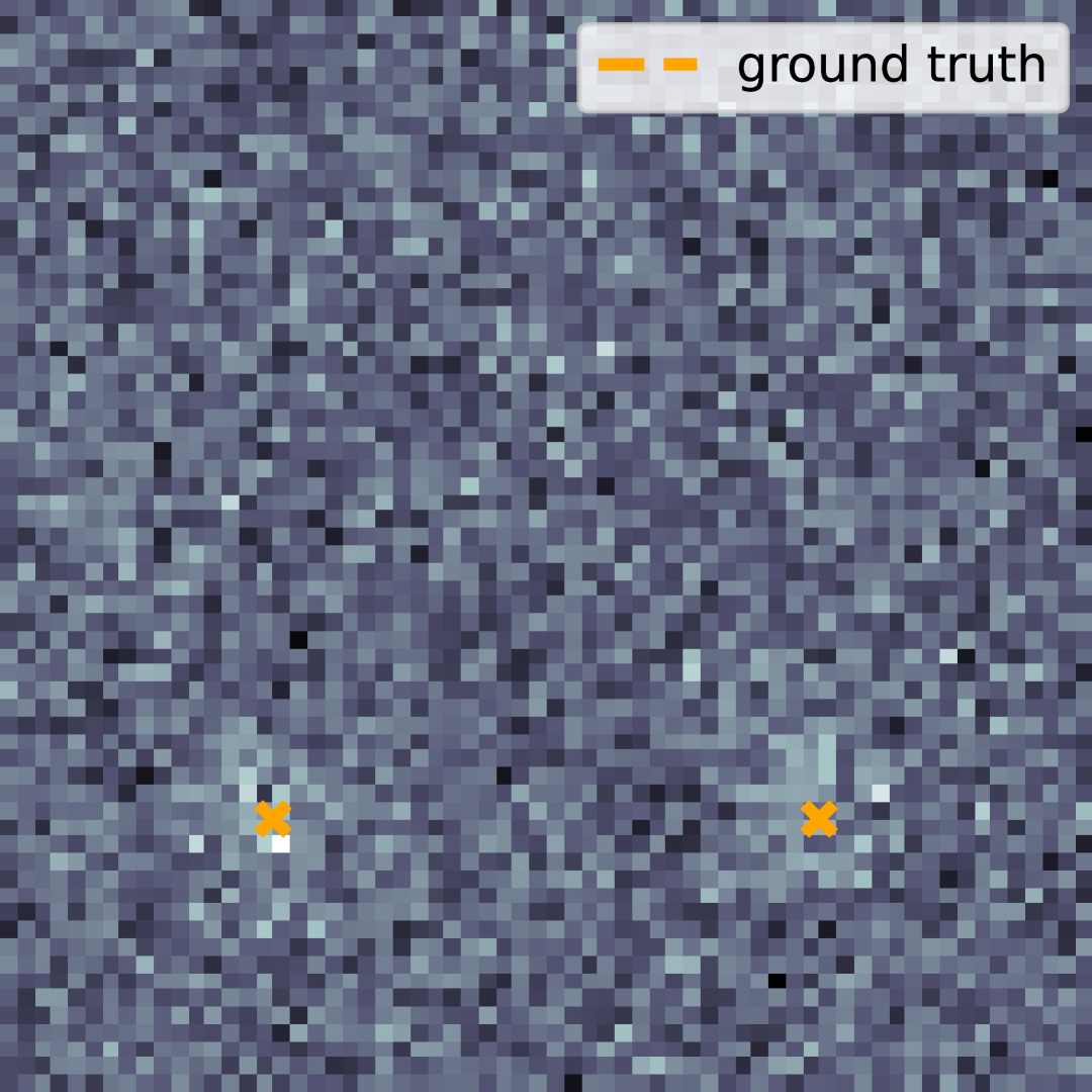
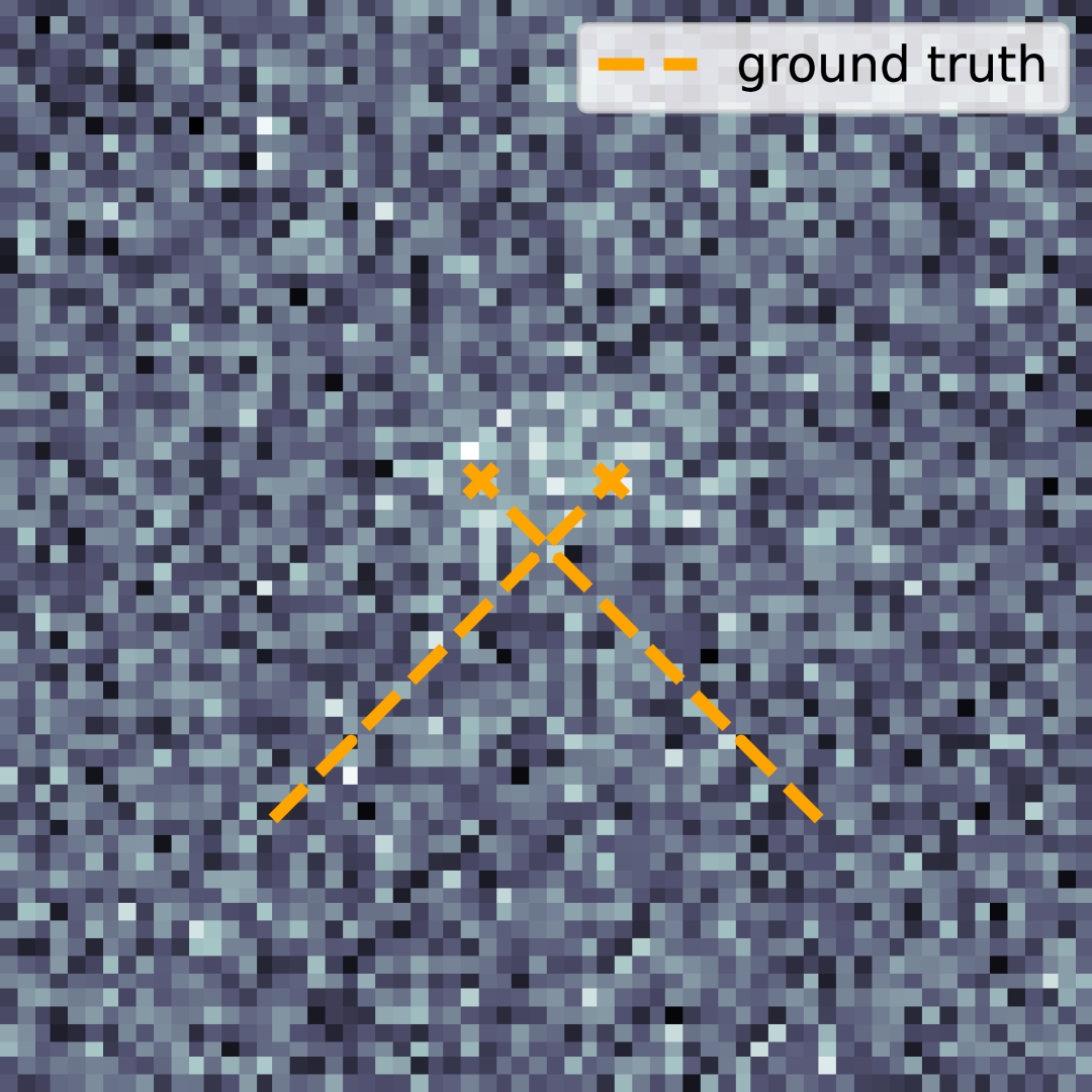
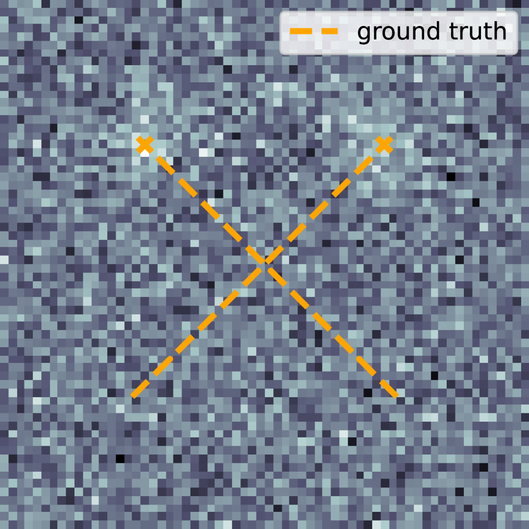
Figure 3: First phantom for $T=21$ frames and two spikes crossing themselves, 60% of white Gaussian noise altering each frame (here at first, half of stack and last frame).

5.2 Balanced optimal transport

We consider two phantoms from [11], the former consists in two point measures crossing, while the latter is a bit more tedious with three Dirac measures moving nearby. The data term is defined as a set of linear forms chosen as the integral of test functions against the temporal measure $\rho_{t}$ at time $t.$ This formulation covers the cases defined in [7] where Fourier coefficients are taken. We chose a classic test function for these synthetic applications by setting the test functions as a Gaussian kernel centred on vertices of a $N\times N$ grid covering $[-1,1]\times[-1,1]$, defined likewise [22]. From an application perspective, this may be seen as a discrete convolution of the measure with the Point Spread Function of the imaging system. The Gaussian spread is set to $\sigma=0.01$ on a $64\times 64$ domain.

The first phantom is generated with $T=21$ time samples, and will be tested on the worst-case scenario, namely 60 noise altering each image: see Figure 3. The regularisation parameter $\beta$ (and so forth $\varepsilon$ and $\xi$) has to be tuned properly.

We present in the figure 4 how different choices reach opposite output, hence the proper choice of these parameters is the crux for the untangling of curves.

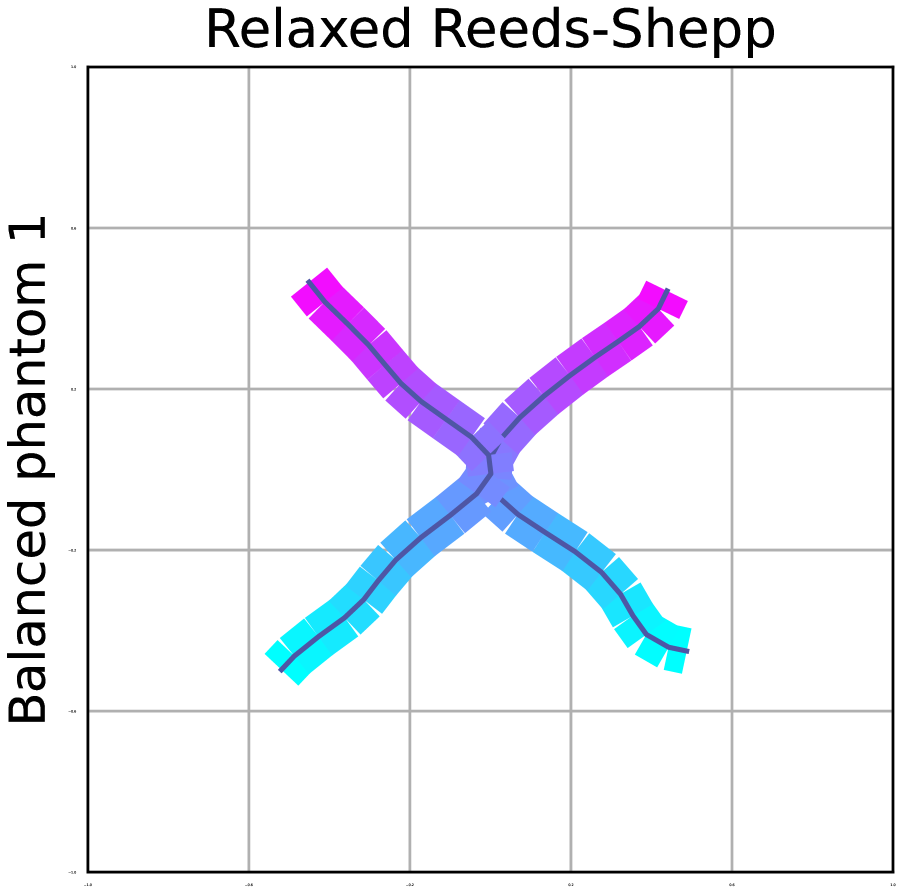
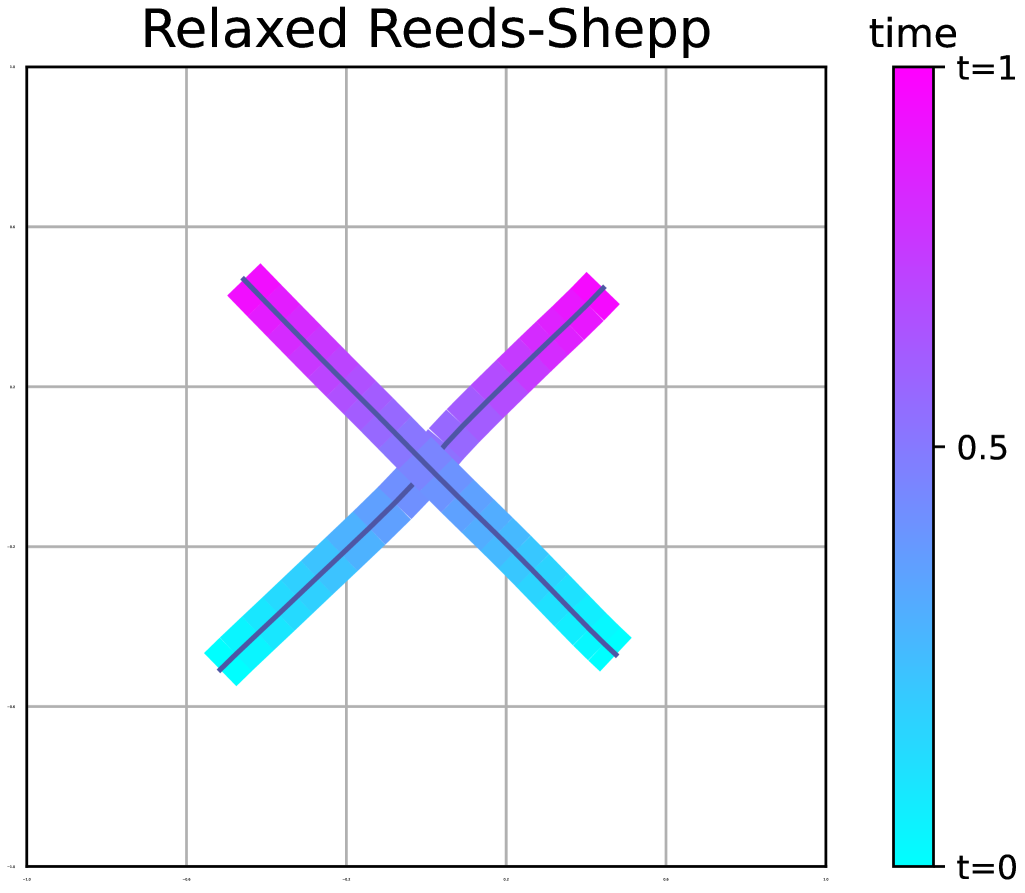
Figure 4: Reconstruction of the first phantom of [11, 25] consisting of a stack of 21 images altered by 60% of Gaussian noise. Each curve is a Bézier curve parametrised by control points living in $\mathbb{M}_{2}$. Left: crossing is not recovered, with $\beta=${10}^{-3}$$, $\varepsilon=$0.5$$ and $\xi=100$. Right: untangling of curves, parameters are tuned to $\beta=${10}^{-3}$$, $\varepsilon=$0.05$$ and $\xi=1$.

In layman terms, we could give the following interpretation:

• $\beta$ controls the regularisation of our Benamou-Brenier flavoured regularisation,

• $\varepsilon$ enforces the planarity of the curve,

• $\xi$ penalises the local curvature.

Our method is then compared with state-of-the-art results from [11, 25] in figure 5. Our algorithm successfully untangles the trajectory, even with the high level of noise. The computation time is approximatively 6 seconds on a Xenon CPU E5-2687W for polygonal, 50 seconds for Bézier and up to 30 minutes for piecise geodesic.

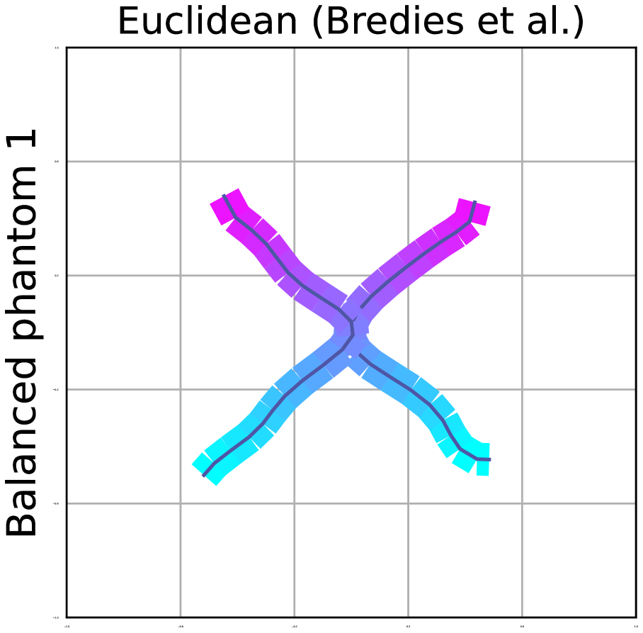
Figure 5: Reconstruction of the first phantom of [11, 25] consisting of a stack of 21 images altered by 60% of Gaussian noise. Left: result from [11], quite similar to [25] up to the speed of convergence, the crossing cannot be recovered. Right: untangling of curves with our method, parameters are tuned to $\beta=${10}^{-5}$$, $\varepsilon=$0.05$$ and $\xi=1$.

The choice of discretisation significantly affects the resulting curves. Bézier curve discretisation facilitates the identification of crossing curves, whereas polygonal discretisations may not. Bézier curves are generally preferred as they are smooth and their non-locality allows for a good expressivity while they are lightweight to compute. Otherwise, piecewise geodesic discretisation bears a higher computation load (by to 2 orders of magnitude) as one needs to solve at each iteration the geodesic equation (6), with the Christoffel symbols in Appendix C, but also yields good results often similar to Bézier ones. In the following, we present only the results on Bézier curves as it shows the best performance, but the reader should feel free to examine the repositories for more information.

The second phantom now consists of $T=51$ slices, where one needs to recover three paths. The results are plotted in figure 6. The computation time is approximately 31 seconds on the Xenon, 2 minutes for Bézier and up to one hour for piecewise geodesic.

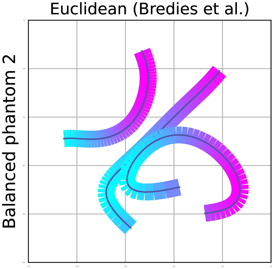
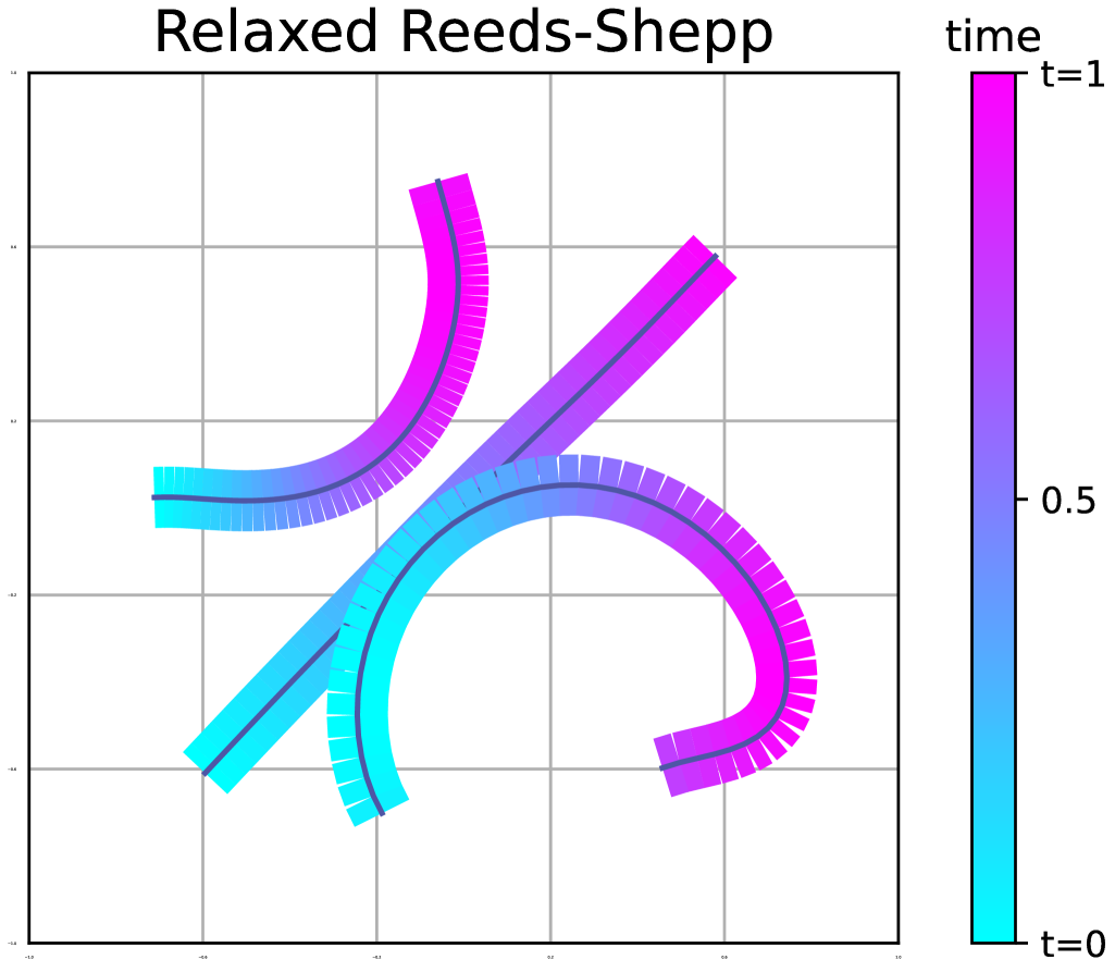
Figure 6: Reconstruction of the second phantom of [11, 25] consisting of a stack of 51 images altered by 60% of Gaussian noise. The ground-truth spikes are not blending in each other, but rather take the same path at different times. Left: result from [11], quite similar to [25] up to the speed of convergence. Right: Reeds-Shepp regularisation, parameters are tuned to $\beta=${10}^{-3}$$, $\varepsilon=$0.05$$ and $\xi=1$.

5.3 Unbalanced optimal transport

Some further developments in the literature [25], among other improvements such as the computation time, proposed to tackle the unbalanced optimal transport case: this encompasses any moving Dirac with varying amplitude over time. This addition is a rather important feature in the biomedical applications, since the molecules of interest can lose brightness over time. Since the mass may change, the regulariser is no longer the Benamou-Brenier energy but the quite similar Wasserstein-Fisher-Rao one, as proposed in [9, 11] from the seminal work of [17, 30, 35]. Hence, the optimisation performed consists of an unbalanced optimal transport.

We propose adding up this idea to our algorithm to handle more general problems. In practice, the amplitude information is implemented in a new dimension added to the control points, the estimated amplitude will thereby be a Bézier curve. For instance, in the case $d=2$, the control points bear 4 dimensions, the first ones for spatial dimension $(x_{1},x_{2})$, the third amounting to the orientation $\theta$ (enabling the curve crossing) and the fourth covering the amplitude $a$ (evolution of the mass over time) values of the curve.

We noticed in our experiments that the algorithm tends to share unfairly the global mass over the estimated paths: there is a ’winner takes it all’ effect, where the algorithm lean in favour of the first estimated curve (overestimating it) while giving less mass to the second curve (underestimating it). As for the original article [25], it did not enforce any prior on the amplitude part and boils down to a least square norm fitting. We propose to add a small regularisation with parameter $\zeta\in\mathbb{R}^{+}$:

$$\mbox{if }{\bm{\gamma}}=\left(x_{1}(t),x_{2}(t),\theta(t),a(t)\right),\quad R({\bm{\gamma}})=\zeta\norm{a}_{2}^{2}.$$

In the practical setting, this regulariser is added to the energy and the energy is optimised accordingly. The case $\zeta=0$ is precisely the classical Wasserstein-Fisher-Rao unbalanced optimal transport from [25]. In the following, we present in figure 7 the reconstruction performed by our method, against the reconstruction in the literature, which lacks by design the curve crossing. Our method successfully captures the dynamic of both paths and amplitudes components, and this latter observation generalises even with noise. Note that in the bottom left corner, our algorithm struggles to recover the ’loose ends’ namely the position where the amplitude of the moving Dirac measure vanishes: the algorithms may handle paths discontinuities by zeroing out the amplitude, but a near-zero amplitude on the path endpoint is hard to capture since there is no connectivity prior to exploit.

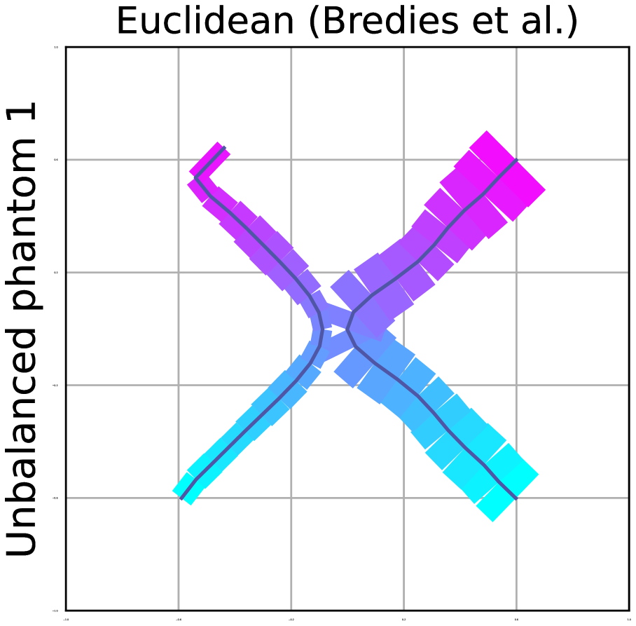
Figure 7: Reconstruction of the first phantom of [11, 25] consisting in a stack of 21 images with varying masses on the paths and 10 % noise. Left: result for $\beta=${10}^{-5}$$ without any lift, the crossing cannot be recovered. Right: untangling of curves with our method, parameters are tuned to $\beta=$6\text{\times}{10}^{-4}$$, $\varepsilon=$0.05$$, $\xi=1$ and $\zeta=0.3\beta$.

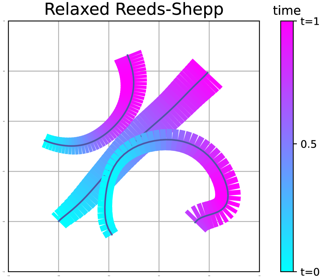
Figure 8: Reconstruction of the second phantom of [11, 25], unbalanced case with 60 % of Gaussian noise. Left: result for $\beta=${10}^{-5}$$. Right: Reeds-Shepp relaxation, parameters are tuned to $\beta=$6\text{\times}{10}^{-4}$$, $\varepsilon=$0.05$$, $\xi=1$ and $\zeta=0.3\beta$.

To sum this up, the Unravelling Frank-Wolfe algorithm is able to recover crossing paths with various discretisations and possibly varying masses over time. Bézier curves perform reasonably well compared to piecewise geodesic discretisation, while being lightweight to compute. In future work, it may be interesting to consider Riemannian Bézier curves compatible with the manifold structure through a definition as the Fréchet mean on the control points on the manifold rather than its current definition, which still relies on the ambient space.

6 Conclusion and outlook

We successfully proposed a method to enable the reconstruction and untangling of crossing moving point sources, through the use of a lift with the roto-translational space $\mathbb{M}_{d}$ and the introduction of a proper metric to untangle the crossing path while controlling the path curvature. This metric, inspired by biomedical applications, has been used as a regularisation term. Then, we proved $\Gamma$-convergence results for discretisation of our proposed energy but not limited to, this may come handy for other off-the-grid curve reconstruction. Eventually, an Unravelling Frank-Wolfe algorithm has been introduced to successfully tackle the augmented problem, through the leveraging of Riemannian structure in both the inner gradient descents and the metric in the objective energy. We also tested discretisations considered in the latter section and proved the capabilities of Bézier curves, compared to piecewise geodesic and polygonal ones.

Still, some difficulties arise naturally, and point out some limitations such as curvature variation: untangling curves requires a precise control on the curvature, which leads to a trade-off between smoothness and entanglement. Fortunately, in real data, the curve structure only bears a rather little curvature, which is encouraging for precise untangling.

In future works, it would be interesting to consider the extension of this method to off-the-grid divergence regularisation known to promote curves [33], namely the reconstruction (and untangling) of curves from one image rather than a stack. Both problems, dynamic path and static curves, share many similarities and could benefit from each other improvements. Also, our proposed algorithm will be tested on real data images, taken from Ultrasound localisation microscopy (ULM) [26, 18] which aims to image this circulation, and relies on multiple image frames containing microbubbles, flowing through the blood vessels as an approximation to the real vasculature. The overall algorithm could be delivered in a so-called ’off-the-shelf’ package, which may come handy for biologists and applicative researchers with a GUI.

7 Acknowledgments

The authors thank Arthur Chavignon for the ULM dataset. They are also deeply grateful to Gilles Aubert and Laure Blanc-Féraud for their time and insightful feedback on the article. BL would like to warmly thank TB for the shelter he provided in his flat back in 2023, and for the pungent yet luscious homemade coffee he got to taste then.

Appendix A Some precisions on geodesic and Riemannian setting

We begin by recommending that the reader review the relevant concepts from differential geometry, as introduced in Section 3.2.1.

Definition A.1.

The metric derivative [2] of an absolutely continuous curve $\gamma\in\mathrm{AC}([0,1],X)$ reads

(8) $$\forall t\in[0,1],\quad|\dot{\gamma}|(t)=\lim_{\eta\to 0}\frac{d(\gamma(t),\gamma(t+\eta))}{|\eta|},$$

and it is the optimal function satisfying (3) as in definition 2.7.

We may now introduce the following lemma, useful in the Riemannian context, see section 3.2.1 for details, .

Lemma A.2.

If the distance $d$ is the Euclidean distance, and $\gamma\in\Gamma$ is differentiable, then the metric derivative corresponds to the norm of the classical derivative : $\forall t\in[0,1],\quad|\dot{\gamma}|(t)=\|\gamma^{\prime}(t)\|_{g}.$

Similarly, if $d$ is the geodesic distance associated with the metric tensor $g$, then the metric derivative corresponds to the metric applied to the classical derivative : $\forall t\in[0,1],\quad|\dot{\gamma}|(t)=\sqrt{g_{\gamma(t)}(\gamma^{\prime}(t),\gamma^{\prime}(t))}.$

Proof A.3.

The Euclidean case comes directly from the definition of the derivative, and the Riemannian case is proven via:

$$\frac{d(\gamma(t),\gamma(t+\eta))}{|\eta|}$$

$$=\frac{\sqrt{g_{\gamma(t)}\left(\operatorname{\mathrm{Log}}_{\gamma(t)}(\gamma(t+\eta)),\operatorname{\mathrm{Log}}_{\gamma(t)}(\gamma(t+\eta))\right)}}{|\eta|}$$

$$=\sqrt{g_{\gamma(t)}\left(\frac{\operatorname{\mathrm{Log}}_{\gamma(t)}(\gamma(t+\eta))-\operatorname{\mathrm{Log}}_{\gamma(t)}(\gamma(t))}{\eta},\frac{\operatorname{\mathrm{Log}}_{\gamma(t)}(\gamma(t+\eta))-\operatorname{\mathrm{Log}}_{\gamma(t)}(\gamma(t))}{\eta}\right)}$$

$$\longrightarrow_{\eta\xrightarrow{}0}\sqrt{g_{\gamma(t)}(\,\mathrm{d}\operatorname{\mathrm{Log}}_{\gamma(t)}\gamma(t)\cdot\gamma^{\prime}(t),\,\mathrm{d}\operatorname{\mathrm{Log}}_{\gamma(t)}\gamma(t)\cdot\gamma^{\prime}(t))}=\sqrt{g_{\gamma(t)}(\gamma^{\prime}(t),\gamma^{\prime}(t))}$$

Appendix B Extremal points of the Benamou-Brenier Energy (Riemannian case)

Lemma B.1.

The functional $w:\gamma\in\Gamma^{\mathcal{M}}\mapsto\int_{0}^{1}\alpha+\beta\left\|\gamma^{\prime}(t)\right\|_{g}\,\mathrm{d}t$, is lower semi-continuous.

Proof B.2.

$w$ may be rewritten as the supremum of a family of continuous functions of $\gamma$ :

$$w(\gamma)=\sup_{t_{0}=0<t_{1}\dots<t_{n}=1}\alpha+\beta\sum_{k=0}^{n-1}\frac{d_{g}(\gamma(t_{k}),\gamma(t_{k+1}))}{t_{k+1}-t_{k}},$$

thus ensuring lower semi-continuity of $w.$

Lemma B.3.

Let $w:\Gamma\xrightarrow{}]0,+\infty]$ a lower semi-continuous function and $D=\left\{\sigma\in\mathcal{M}(\Gamma)/\int_{\Gamma}w\,\mathrm{d}\sigma\leq 1\right\}.$ D is closed and:

$$\mathrm{Ext}(D)=\{0\}\cup\left\{w(\gamma)^{-1}\delta_{\gamma}\,|\,w(\gamma)<+\infty\right\}.$$

Proof B.4.

For any convex decomposition $\sigma=\lambda\sigma_{1}+(1-\lambda)\sigma_{2},$ if $\sigma=w(\gamma)^{-1}\delta_{\gamma}$ for any $\gamma\in\Gamma,$ then $\sigma_{1}$ and $\sigma_{2}$ are supported only on $\gamma$, i.e. there exists $\alpha,\beta\in\mathbb{R}_{+}$ such that $\quad\sigma_{1}=\frac{\alpha}{w(\gamma)}\delta_{\gamma},\quad\sigma_{2}=\frac{\beta}{w(\gamma)}\delta_{\gamma}$.
And then, as $\int w\,\mathrm{d}\sigma=1=\lambda\alpha+(1-\lambda)\beta$ and $\alpha+\beta=1,$ we have $\alpha=\beta=1$ and $\sigma=\sigma_{1}=\sigma_{2}$. Hence, $w(\gamma)^{-1}\delta_{\gamma}$ is indeed an extremal point of $D.$

Let $\sigma\in\mathrm{Ext}(D),$ and make the assumption that there are at least 2 curves $\gamma_{0}$ and $\gamma_{1}$ in the support of $\sigma.$ Let $\Gamma_{0}=\{d_{\Gamma}(\gamma,\gamma_{0})\leq\frac{1}{2}d_{\Gamma}(\gamma_{1},\gamma_{0})\},$ and $\Gamma_{1}=\Gamma_{0}^{c},$ defining $\sigma_{0}=\mathbbm{1}_{\Gamma_{0}}\sigma$ and $\sigma_{1}=\sigma-\sigma_{0}.$
If $\int w\,\mathrm{d}\sigma_{i}\neq 0$ and $\int w\,\mathrm{d}\sigma_{i}\leq\int w\,\mathrm{d}\sigma\leq 1,$ then with $\lambda=\int w\,\mathrm{d}\sigma_{0},$ we get that $\sigma=\lambda\frac{\sigma_{0}}{\lambda}+(1-\lambda)\frac{\sigma_{1}}{1-\lambda}$ and we have written $\sigma$ as a convex combination of elements of $D,$ so either $\sigma\notin\mathrm{Ext}(D)$ or for a certain $i\in\{0,1\},\int w\,\mathrm{d}\sigma_{i}=0.$ In the last case we have that by positivity of $w,$ $\sigma=0$ and then we can’t have $\gamma_{i}\in\Gamma_{i},$ which contradicts the assumption. Thus, we have that $\sigma$ has at most $1$ curve in its support which means either $\sigma=0$ or $\sigma=\frac{1}{w(\gamma)}\delta_{\gamma}$ for some $\gamma\in\Gamma.$

Appendix C Reeds-Shepp metric tensor and its affine connection

Let $p=(x,y,\theta)\in\mathbb{M}_{2}$ a rototranslation, the metric tensor $g$ at $p$ is defined by:

$$g_{ij}=\begin{bmatrix}\cos(\theta)^{2}+\varepsilon^{-2}\sin(\theta)^{2}&\left(1-\varepsilon^{-2}\right)\cos(\theta)\sin(\theta)&0\\ \left(1-\varepsilon^{-2}\right)\cos(\theta)\sin(\theta)&\sin(\theta)^{2}+\varepsilon^{-2}\cos(\theta)^{2}&0\\ 0&0&\xi^{2}\end{bmatrix},$$

with constants $\varepsilon,\xi>0$ while its contravariant inverse reads:

$$g^{ij}=\begin{bmatrix}\cos(\theta)^{2}+\varepsilon^{2}\sin(\theta)^{2}&\left(1-\varepsilon^{2}\right)\cos(\theta)\sin(\theta)&0\\ \left(1-\varepsilon^{2}\right)\cos(\theta)\sin(\theta)&\sin(\theta)^{2}+\varepsilon^{2}\cos(\theta)^{2}&0\\ 0&0&\xi^{-2}\end{bmatrix}.$$

The Christoffel symbols, up to the symmetries $\Gamma^{k}_{ij}=\Gamma^{k}_{ji}$ and the null symbols, of the Levi-Civita connection $\operatorname{\gradient}$ associated to $g$ write down:

$$\Gamma^{x}_{x,\theta} =-\frac{1}{2\varepsilon^{2}}(\varepsilon^{4}-1)\cos(\theta)\sin(\theta)$$

$$\Gamma^{x}_{y,\theta} =-\frac{1}{2\varepsilon^{2}}(\varepsilon^{4}-(\varepsilon^{4}-1)\cos(\theta)^{2}-\varepsilon^{2})$$

$$\Gamma^{y}_{x,\theta} =\frac{1}{2\varepsilon^{2}}((\varepsilon^{4}-1)\cos(\theta)^{2}-\varepsilon^{2}+1)$$

$$\Gamma^{y}_{y,\theta} =\frac{\varepsilon^{4}-1}{2\varepsilon^{2}}\cos(\theta)\sin(\theta)$$

$$\Gamma^{\theta}_{x,x} =\frac{\varepsilon^{2}-1}{\varepsilon^{2}\xi^{2}}\cos(\theta)\sin(\theta)$$

$$\Gamma^{\theta}_{x,y} =-\frac{1}{2\varepsilon^{2}\xi^{2}}(2(\varepsilon^{2}-1)\cos(\theta)^{2}-\varepsilon^{2}+1)$$

$$\Gamma^{\theta}_{y,y} =-\frac{\varepsilon^{2}-1}{\varepsilon^{2}\xi^{2}}\cos(\theta)\sin(\theta).$$

Appendix D Riemannian optimization on manifold and tangent bundle

D.1 Improved gradient descent by the Riemannian structure

For first-order optimization, there is a simple adaptation of gradient descent for Riemannian manifold $(\mathcal{M},g)$. The Riemannian gradient descent simply consists in a gradient descent, but we take into account the non-Euclidean nature of the manifold by leveraging the Riemannian exponential map to ramp the update on the manifold. The procedure is described in Algorithm 2.

Input: Objective function $f:x\in\mathcal{M}\mapsto f(x)\in\mathbb{R}$, initialisation point $x_{0}\in\mathcal{M}$, number of timesteps $T\in\mathbb{N}^{*}$

1

2for $t=0,1,2,\ldots,T-1$ do

3    Compute the Riemannian gradient $\nabla_{\mathcal{M}}f(x)$.

4   Update the iterate by:

$$x=\operatorname{\mathrm{Exp}}_{x}(-\eta\nabla_{\mathcal{M}}f(x))$$

where $\text{Exp}_{x}$ denotes the Riemannian exponential map at point $x$.

5 end for

Output: Point $x$ of the manifold

6

Algorithm 2 Riemannian gradient descent

Usually, we replace the use of the exponential map by a retraction, i.e. a first-order approximation of this mapping.

D.2 Optimisation on the tangent bundle

Now, we want to carry out the Riemannian gradient descent not only on the base manifold itself but also on the tangent bundle, which means that the objective function is now the mapping:

$$f:(x,v)\in\mathcal{M}\times\mathcal{T}_{x}\mathcal{M}\mapsto f(x,v)\in\mathbb{R}.$$

The tangent bundle $\mathcal{T}\mathcal{M}$ is itself a $2d$–dimensional manifold with tangent bundle $\mathcal{T}\mathcal{T}\mathcal{M}.$ For any base point $(p,u)\in\mathcal{T}\mathcal{M},$ $\mathcal{T}_{(p,u)}\mathcal{T}\mathcal{M}$ has a particular structure [38] as it can be decomposed into horizontal and vertical subspaces, both $d-$dimensional:

$$\mathcal{T}_{(p,u)}\mathcal{T}\mathcal{M}=\mathcal{H}_{(p,u)}\oplus\mathcal{V}_{(p,u)},$$

There exists a natural lift from $\mathcal{T}_{p}\mathcal{M}$ to the horizontal and vertical subspaces, let $X\in\mathcal{T}_{p}\mathcal{M}$ we denote $X^{h}$ the horizontal part and $X^{v}$ the vertical part of $X$.

A natural choice of metric for the tangent bundle manifold is called the Sasaki metric [38]. It simply consists in using the base metric and imposing perpendicularity of the horizontal and vertical subspaces, i.e. ensuring that the horizontal and vertical subspaces remain orthogonal.

Definition D.1.

The Sasaki metric $\operatorname{\hat{g}}$ is a metric on $\mathcal{T}_{(p,u)}\mathcal{T}\mathcal{M}$ derived from the base metric $g$ by the following properties.

1. Horizontal reservation of the metric: $\operatorname{\hat{g}}_{(p,u)}(X^{h},Y^{h})=g_{p}(X,Y),$

2. Vertical preservation of the metric: $\operatorname{\hat{g}}_{(p,u)}(X^{v},Y^{v})=g_{p}(X,Y),$

3. Orthogonality: $\operatorname{\hat{g}}_{(p,u)}(X^{h},Y^{v})=0,$

D.3 Energy in the piecewise geodesic framework on the Sasaki metric

For ease of implementation and instead of the straightforward piecewise geodesic model, we consider a set of points on the Sasaki manifold associated with the base Reeds-Shepp metric $(x_{k},v_{k})_{1\leq k\leq n-1}$. The piecewise geodesic curve interpolating the points corresponds to the condition, $\forall 1\leq k\leq n-1$: $\operatorname{\mathrm{Exp}}_{x_{k}}(v_{k})=x_{k+1}$.

We bring slight modifications to the energy by simply adding a penalisation, to avoid the difficult and expensive computation of the Riemannian Log map.

Finally, the energy we minimise in the oracle step writes down, for $\lambda>0$:

$$F((x_{k},v_{k})) =-\braket{\gamma_{(x_{k},v_{k})},\eta^{[k]}}_{\mathcal{M}(\Gamma)}+\beta\sum_{k}(t_{k+1}-t_{k})\,\norm{v_{k}}_{x_{k}}^{2}$$

$$\quad+\lambda\sum_{k}\norm{\operatorname{\mathrm{Exp}}_{x_{k}}(v_{k})-x_{k+1}}_{2}^{2}.$$

References

- [1] A. Agrachev, D. Barilari, and U. Boscain, A Comprehensive Introduction to sub-Riemannian Geometry, Cambridge University Press, 2020, https://hal.science/hal-02019181. Introduction de l’ouvrage.
- [2] L. Ambrosio, N. Gigli, and G. Savare, Gradient Flows in Metric Spaces and in the Space of Probability Measures, Springer-Verlag GmbH, 2008, https://doi.org/10.1007/978-3-7643-8722-8, https://www.ebook.de/de/product/8899095/giuseppe_savare_luigi_ambrosio_nicola_gigli_gradient_flows.html.
- [3] E. Bekkers, R. Duits, T. Berendschot, and B. ter Haar Romeny, A multi-orientation analysis approach to retinal vessel tracking, Journal of Mathematical Imaging and Vision, 49 (2014), pp. 583–610, https://doi.org/10.1007/s10851-013-0488-6, https://doi.org/10.1007/s10851-013-0488-6.
- [4] E. J. Bekkers, R. Duits, A. Mashtakov, and G. R. Sanguinetti, A pde approach to data-driven sub-riemannian geodesics in SE(2), SIAM Journal on Imaging Sciences, 8 (2015), pp. 2740–2770, https://doi.org/10.1137/15M1018460, https://doi.org/10.1137/15M1018460, https://arxiv.org/abs/https://doi.org/10.1137/15M1018460.
- [5] C. Boyer, A. Chambolle, Y. D. Castro, V. Duval, F. de Gournay, and P. Weiss, On representer theorems and convex regularization, SIAM Journal on Optimization, 29 (2019), pp. 1260–1281, https://doi.org/10.1137/18m1200750, https://arxiv.org/abs/1806.09810.
- [6] A. Braides, Gamma-convergence for Beginners, Oxford University Press, USA, 2002.
- [7] K. Bredies and M. Carioni, Sparsity of solutions for variational inverse problems with finite-dimensional data, Calculus of Variations and Partial Differential Equations, 59 (2019), https://doi.org/10.1007/s00526-019-1658-1, https://arxiv.org/abs/1809.05045.
- [8] K. Bredies, M. Carioni, and S. Fanzon, A superposition principle for the inhomogeneous continuity equation with hellinger–kantorovich-regular coefficients, Communications in Partial Differential Equations, 47 (2022), p. 2023–2069, https://doi.org/10.1080/03605302.2022.2109172, http://dx.doi.org/10.1080/03605302.2022.2109172.
- [9] K. Bredies, M. Carioni, S. Fanzon, and F. Romero, On the extremal points of the ball of the benamou–brenier energy, Bulletin of the London Mathematical Society, (2021), https://doi.org/10.1112/blms.12509, https://arxiv.org/abs/1907.11589.
- [10] K. Bredies, M. Carioni, S. Fanzon, and F. Romero, A generalized conditional gradient method for dynamic inverse problems with optimal transport regularization, Foundations of Computational Mathematics, (2022), https://doi.org/10.1007/s10208-022-09561-z, https://arxiv.org/abs/2012.11706.
- [11] K. Bredies and S. Fanzon, An optimal transport approach for solving dynamic inverse problems in spaces of measures, ESAIM: Mathematical Modelling and Numerical Analysis, 54 (2020), p. 2351–2382, https://doi.org/10.1051/m2an/2020056, http://dx.doi.org/10.1051/m2an/2020056.
- [12] K. Bredies and H. K. Pikkarainen, Inverse problems in spaces of measures, ESAIM: Control, Optimisation and Calculus of Variations, 19 (2012), pp. 190–218, https://doi.org/10.1051/cocv/2011205.
- [13] E. Cartan, Leçons sur la géométrie des espaces de Riemann, Mémorial des sciences mathématiques, 1946.
- [14] Y. D. Castro, F. Gamboa, D. Henrion, and J.-B. Lasserre, Exact solutions to super resolution on semi-algebraic domains in higher dimensions, IEEE Transactions on Information Theory, 63 (2017), pp. 621–630, https://doi.org/10.1109/tit.2016.2619368, https://arxiv.org/abs/1502.02436.
- [15] A. Chambolle and T. Pock, Total roto-translational variation, Numerische Mathematik, 142 (2019), pp. 611–666, https://doi.org/10.1007/s00211-019-01026-w, https://arxiv.org/abs/1709.09953.
- [16] L. Chizat, Sparse optimization on measures with over-parameterized gradient descent, Mathematical Programming, (2021), https://doi.org/10.1007/s10107-021-01636-z, https://arxiv.org/abs/1907.10300.
- [17] L. Chizat, G. Peyré, B. Schmitzer, and F.-X. Vialard, An interpolating distance between optimal transport and fisher–rao metrics, Foundations of Computational Mathematics, 18 (2016), p. 1–44, https://doi.org/10.1007/s10208-016-9331-y, http://dx.doi.org/10.1007/s10208-016-9331-y.
- [18] O. Couture, V. Hingot, B. Heiles, P. Muleki-Seya, and M. Tanter, Ultrasound localization microscopy and super-resolution: A state of the art, IEEE Transactions on Ultrasonics, Ferroelectrics, and Frequency Control, 65 (2018), pp. 1304–1320, https://doi.org/10.1109/tuffc.2018.2850811.
- [19] Y. de Castro, V. Duval, and R. Petit, Towards off-the-grid algorithms for total variation regularized inverse problems, in Lecture Notes in Computer Science, Springer International Publishing, 2021, pp. 553–564, https://arxiv.org/abs/2104.06706.
- [20] Y. de Castro and F. Gamboa, Exact reconstruction using beurling minimal extrapolation, Journal of Mathematical Analysis and Applications, 395 (2012), pp. 336–354, https://doi.org/10.1016/j.jmaa.2012.05.011, https://arxiv.org/abs/1103.4951.
- [21] Q. Denoyelle, V. Duval, and G. Peyré, Support Recovery for Sparse Super-Resolution of Positive Measures, Journal of Fourier Analysis and Applications, (2016), https://doi.org/10.1007/s00041-016-9502-x, https://hal.archives-ouvertes.fr/hal-01270184.
- [22] Q. Denoyelle, V. Duval, G. Peyré, and E. Soubies, The sliding frank–wolfe algorithm and its application to super-resolution microscopy, Inverse Problems, 36 (2019), p. 014001, https://doi.org/10.1088/1361-6420/ab2a29, https://arxiv.org/abs/1811.06416.
- [23] R. Duits, S. P. Meesters, J.-M. Mirebeau, and J. M. Portegies, Optimal paths for variants of the 2d and 3d reeds–shepp car with applications in image analysis, Journal of Mathematical Imaging and Vision, 60 (2018), pp. 816–848.
- [24] V. Duval and G. Peyré, Exact support recovery for sparse spikes deconvolution, Foundations of Computational Mathematics, 15 (2014), pp. 1315–1355, https://doi.org/10.1007/s10208-014-9228-6, https://arxiv.org/abs/1306.6909.
- [25] V. Duval and R. Tovey, Dynamical programming for off-the-grid dynamic inverse problems, ESAIM: Control, Optimisation and Calculus of Variations, 30 (2024), p. 7, https://doi.org/10.1051/cocv/2023085, http://dx.doi.org/10.1051/cocv/2023085.
- [26] C. Errico, J. Pierre, S. Pezet, Y. Desailly, Z. Lenkei, O. Couture, and M. Tanter, Ultrafast ultrasound localization microscopy for deep super-resolution vascular imaging, Nature, 527 (2015), p. 499–502, https://doi.org/10.1038/nature16066.
- [27] H. Federer, Geometric measure theory, Springer, Berlin, 1996.
- [28] M. Frank and P. Wolfe, An algorithm for quadratic programming, Naval Research Logistics Quarterly, 3 (1956), pp. 95–110, https://doi.org/10.1002/nav.3800030109.
- [29] S. Gudmundsson and E. Kappos, On the geometry of tangent bundles, Expositiones Mathematicae, 20 (2002), pp. 1–41, https://doi.org/https://doi.org/10.1016/S0723-0869(02)80027-5, https://www.sciencedirect.com/science/article/pii/S0723086902800275.
- [30] S. Kondratyev, L. Monsaingeon, and D. Vorotnikov, A new optimal transport distance on the space of finite radon measures, Advances in Differential Equations, 21 (2016), https://doi.org/10.57262/ade/1476369298, http://dx.doi.org/10.57262/ade/1476369298.
- [31] B. Laville, L. Blanc-Féraud, and G. Aubert, A -convergence result and an off-the-grid charge algorithm for curve reconstruction in inverse problems, Journal of Mathematical Imaging and Vision, 66 (2024), pp. 572–583.
- [32] B. Laville, L. Blanc-Féraud, and G. Aubert, Off-The-Grid Variational Sparse Spike Recovery: Methods and Algorithms, Journal of Imaging, 7 (2021), p. 266, https://doi.org/10.3390/jimaging7120266.
- [33] B. Laville, L. Blanc-Féraud, and G. Aubert, Off-the-grid curve reconstruction through divergence regularization: An extreme point result, SIAM Journal on Imaging Sciences, 16 (2023), p. 867–885, https://doi.org/10.1137/22m1494373, http://dx.doi.org/10.1137/22M1494373.
- [34] J. M. Lee, Introduction to Riemannian manifolds, Graduate texts in mathematics, Springer International Publishing, Cham, Switzerland, 2 ed., Jan. 2019.
- [35] M. Liero, A. Mielke, and G. Savaré, Optimal entropy-transport problems and a new hellinger–kantorovich distance between positive measures, Inventiones mathematicae, 211 (2017), p. 969–1117, https://doi.org/10.1007/s00222-017-0759-8.
- [36] G. Maso, An Introduction to -Convergence, Progress in Nonlinear Differential Equations and Their Applications, Birkhäuser Boston, 2012, https://books.google.fr/books?id=7bkGCAAAQBAJ.
- [37] J. Reeds and L. Shepp, Optimal paths for a car that goes both forwards and backwards, Pacific Journal of Mathematics, 145 (1990), pp. 367–393, https://doi.org/10.2140/pjm.1990.145.367.
- [38] S. Sasaki, On the differential geometry of tangent bundles of riemannian manifolds, Tohoku Mathematical Journal, 10 (1958), https://doi.org/10.2748/tmj/1178244668, http://dx.doi.org/10.2748/tmj/1178244668.
- [39] B. Schmitzer, K. P. Schafers, and B. Wirth, Dynamic cell imaging in pet with optimal transport regularization, IEEE Transactions on Medical Imaging, 39 (2020), p. 1626–1635, https://doi.org/10.1109/tmi.2019.2953773, http://dx.doi.org/10.1109/TMI.2019.2953773.
- [40] E. Schrodinger, Cambridge science classics: Space-time structure, Cambridge University Press, Cambridge, England, Dec. 2009.