Efficient Parametric SVD of Koopman Operator
for Stochastic Dynamical Systems

Abstract

The Koopman operator provides a principled framework for analyzing nonlinear dynamical systems through linear operator theory. Recent advances in dynamic mode decomposition (DMD) have shown that trajectory data can be used to identify dominant modes of a system in a data-driven manner. Building on this idea, deep learning methods such as VAMPnet and DPNet have been proposed to learn the leading singular subspaces of the Koopman operator. However, these methods require backpropagation through potentially numerically unstable operations on empirical second moment matrices, such as singular value decomposition and matrix inversion, during objective computation, which can introduce biased gradient estimates and hinder scalability to large systems. In this work, we propose a scalable and conceptually simple method for learning the top-$k$ singular functions of the Koopman operator for stochastic dynamical systems based on the idea of low-rank approximation. Our approach eliminates the need for unstable linear algebraic operations and integrates easily into modern deep learning pipelines. Empirical results demonstrate that the learned singular subspaces are both reliable and effective for downstream tasks such as eigen-analysis and multi-step prediction.

1 Introduction

The Koopman operator theory offers a powerful framework for analyzing nonlinear dynamical systems by lifting them into an infinite-dimensional function space, where spectral techniques from linear operator theory can be applied. Recent advances in dynamic mode decomposition (DMD) have shown that trajectory data can be effectively used to identify dominant dynamical modes in a data-driven manner (Tu et al., 2014; Williams et al., 2014, 2015; Kutz et al., 2016; Colbrook et al., 2023). Inspired by the success of deep learning, recent methods such as VAMPnet (Wu and Noé, 2020; Mardt et al., 2018) and DPNet (Kostic et al., 2024a) employ neural networks to approximate the leading singular subspaces of the Koopman operator. While shown effective for some benchmark tasks, these approaches often rely on numerically unstable operations such as singular value decomposition (SVD) or matrix inversion during objective computation. These operations present practical challenges, particularly in computing unbiased gradients and scaling to high-dimensional systems.

In this work, we propose a conceptually simple and scalable method for learning the top-$k$ singular functions of the Koopman operator for stochastic dynamical systems. Our approach builds on the idea of low-rank approximation, which has recently received attention in the literature due to its favorable optimization structure that aligns well with modern optimization practices; see, e.g., (Liu et al., 2015; Wen et al., 2016) in the numerical optimization literature, and (Wang et al., 2019; HaoChen et al., 2021; Ryu et al., 2024; Xu and Zheng, 2024; Kostic et al., 2024b) in the machine learning literature. Our method avoids unstable linear algebraic computations and is easy to integrate into modern deep learning pipelines. We demonstrate that it reliably recovers dominant Koopman subspaces and supports downstream tasks such as prediction and eigen-analysis.

2 Problem Setting and Preliminaries

In this section, we introduce the problem setting and establish the foundation for the subsequent discussion. We begin by formulating the problem in the context of discrete-time dynamical systems, which will serve as our primary focus. We then briefly address the continuous-time case. Next, we review two existing approaches, VAMPnet and DPNet, and highlight their limitations, thereby motivating the need for our proposed method.

2.1 Discrete-Time Dynamical Systems

Consider a stochastic discrete-time dynamical system $\mathbf{x}_{t+1}=\xi(\mathbf{F}(\mathbf{x}_{t}),\epsilon_{t})$, where $\mathbf{F}\colon\mathcal{X}\to\mathcal{X}$ is a possibly nonlinear mapping for a domain $\mathcal{X}\subseteq\mathbb{R}^{d}$, $\epsilon_{t}\sim\mathcal{D}$ is an independent noise random variable, and $\mathbf{x}_{t}\mapsto\xi(\mathbf{F}(\mathbf{x}_{t}),\epsilon_{t})\in\mathcal{X}$ captures an independent noise in the process, such as the additive white Gaussian noise. Assuming that $\mathbf{F}$ and the noise distribution $\mathcal{D}$ are time-invariant, the process becomes a time-homogeneous Markov process with transition density $p(\mathbf{x}^{\prime}\mid\mathbf{x})$, i.e., $\Pr(\mathbf{X}_{t+1}\in A\mid\mathbf{X}_{t}=\mathbf{x})=\int_{A}p(\mathbf{x}^{\prime}\mid\mathbf{x})\,d\mathbf{x}^{\prime}$ for all measurable sets $A\subseteq\mathcal{X}$ and all $t\geq 0$.

In the stochastic setup, the dynamics is fully captured by the transition density $p(\mathbf{x}^{\prime}|\mathbf{x})$, which is induced by $(\xi\circ\mathbf{F})(\cdot)$, and thus the problem becomes analyzing $p(\mathbf{x}^{\prime}|\mathbf{x})$ of a Markov chain. Here, the Koopman operator becomes the conditional expectation operator. That is, for an observable $g\colon\mathcal{X}\to\mathbb{R}$, we can write

$$(\mathpzc{K}g)(\mathbf{x})\triangleq\mathbb{E}_{p(\mathbf{x}^{\prime}|\mathbf{x})}[g(\mathbf{x}^{\prime})].$$

By the Markov property, repeatedly applying the Koopman operator will correspond to the multi-step prediction in the sense that it captures the posterior mean of $g(\mathbf{x}_{t})$ given $\mathbf{x}_{0}=\mathbf{x}_{0}$, i.e., $(\mathpzc{K}^{t}g)(\mathbf{x}_{0})=\mathbb{E}_{p(\mathbf{x}_{t}|\mathbf{x}_{0})}[g(\mathbf{x}_{t})]$.

Throughout the paper, we will assume that $\mathpzc{K}$ is compact following (Kostic et al., 2024a), which is a mild assumption that holds for a large class of Markov processes; see, e.g., (Kostic et al., 2022). We remark that we cannot directly apply the existing spectral techniques to a deterministic dynamical system, including the technique developed in this paper, since the corresponding Koopman operator is neither Hilbert–Schmidt nor compact; see (Wu and Noé, 2020, Appendix A.5). Considering stochasticity breaks the degeneracy and allow the linear algebraic techniques applicable. Moreover, assuming stochasticity is not necessarily a restrictive assumption, as physical processes in the real-world may be inherently noisy.

Problem Setting. Our goal is to analyze the Markov dynamics of the length-$T$ trajectory $(\mathbf{x}_{0},\mathbf{x}_{1},\ldots,\mathbf{x}_{T})\sim p(\mathbf{x}_{0})p(\mathbf{x}_{1}|\mathbf{x}_{0})\ldots p(\mathbf{x}_{T}|\mathbf{x}_{T-1})$, where $p(\mathbf{x}_{0})$ is a distribution for the initial state. In practice, we assume that we have access to $N$ independent, random trajectories, and collect the consecutive transition pairs $\{(\mathbf{x}_{0},\mathbf{x}_{1}),(\mathbf{x}_{1},\mathbf{x}_{2}),\dots,(\mathbf{x}_{T-1},\mathbf{x}_{T})\}$ and define the joint distribution over the pair as $p(\mathbf{x},\mathbf{x}^{\prime})\triangleq\frac{1}{T}\sum_{t=0}^{T-1}p_{t}(\mathbf{x})p(\mathbf{x}^{\prime}|\mathbf{x})$, where $p_{0}(\mathbf{x})=p(\mathbf{x}_{0})$ and $p_{t+1}(\mathbf{x}^{\prime})\triangleq\int p(\mathbf{x}^{\prime}|\mathbf{x})p_{t}(\mathbf{x})d\mathbf{x}$. We let $\rho_{0}(\mathbf{x})$ and $\rho_{1}(\mathbf{x}^{\prime})$ denote the marginal distribution over $\mathcal{X}$ of the current and future states. Note that while $\rho_{1}(\mathbf{x}^{\prime})=\mathbb{E}_{\rho_{0}(\mathbf{x})}[p(\mathbf{x}^{\prime}|\mathbf{x})]$ holds, the two distributions, $\rho_{0}(\mathbf{x})$ and $\rho_{1}(\mathbf{x}^{\prime})$ can differ significantly, particularly when the trajectory length $T$ is relatively short.

Let $(\mathcal{X},\mathcal{F})$ be a measurable space and let $\rho_{0}$ and $\rho_{1}$ be (finite) measures on $(\mathcal{X},\mathcal{F})$ representing the distributions of the current and future states, respectively. For any measure $\rho$ on $(\mathcal{X},\mathcal{F})$ define $L_{\rho}^{2}(\mathcal{X})\triangleq\{f\colon\mathcal{X}\to\mathbb{C}|\int|f(\mathbf{x})|^{2}\rho(d\mathbf{x})<\infty\}$. Equipped with the inner product $\langle f,g\rangle_{\rho}\triangleq\int f(\mathbf{x})g(\mathbf{x})\rho(d\mathbf{x})$, $L_{\rho}^{2}(\mathcal{X})$ is a Hilbert space. The Koopman operator $\mathpzc{K}$ is then a mapping from $L_{\rho_{1}}^{2}(\mathcal{X})$ to $L_{\rho_{0}}^{2}(\mathcal{X})$, which is an integral kernel operator with the transition kernel $k(\mathbf{x},\mathbf{x}^{\prime})\triangleq\frac{p(\mathbf{x}^{\prime}|\mathbf{x})}{\rho_{1}(\mathbf{x}^{\prime})}$. The adjoint operator of $\mathpzc{K}^{*}$ then acts as the backward predictor, i.e., $(\mathpzc{K}^{*}f)(\mathbf{x}^{\prime})=\mathbb{E}_{q(\mathbf{x}|\mathbf{x}^{\prime})}[f(\mathbf{x})]$, where $q(\mathbf{x}|\mathbf{x}^{\prime})\triangleq\frac{\rho_{0}(\mathbf{x})p(\mathbf{x}^{\prime}|\mathbf{x})}{\rho_{1}(\mathbf{x}^{\prime})}$ denotes the conditional distribution induced by $\rho_{0}(\mathbf{x})p(\mathbf{x}^{\prime}|\mathbf{x})$. Similar to $\mathpzc{K}$, repeated application of $\mathpzc{K}^{*}$ yields multi-step backward prediction: $((\mathpzc{K}^{*})^{t}f)(\mathbf{x}_{0})=\mathbb{E}_{p(\mathbf{x}_{0}|\mathbf{x}_{t})}[f(\mathbf{x}_{0})].$

Special Case 1: Stationary Markov Processes. Given $p(\mathbf{x}^{\prime}|\mathbf{x})$, let $\pi(\mathbf{x})$ denote the stationary distribution, i.e., the distribution satisfies $\mathbb{E}_{\pi(\mathbf{x})}[p(\mathbf{x}^{\prime}|\mathbf{x})]=\pi(\mathbf{x}^{\prime})$. Under mild regularity conditions such as ergodicity and irreducibility, such distribution exists and is unique. In the stationary case, the marginal distributions at both times are equal, i.e., $\rho_{0}=\rho_{1}=\pi$, and the Koopman operator $\mathpzc{K}$ becomes a map from $L_{\pi}^{2}(\mathcal{X})$ to $L_{\pi}^{2}(\mathcal{X})$. Assuming ergodicity, we can collect the time-lagged pairs $(\mathbf{x},\mathbf{x}^{\prime})$’s from a long, single trajectory, as time averages converge to expectations under the stationary distribution.

Special Case 2: Reversible Markov Processes. A Markov process is time-reversible if and only if it satisfies the detailed balance condition: the joint function $P(\mathbf{x},\mathbf{x}^{\prime})\triangleq\pi(\mathbf{x})p(\mathbf{x}^{\prime}|\mathbf{x})$ is symmetric, i.e., $P(\mathbf{x},\mathbf{x}^{\prime})=P(\mathbf{x}^{\prime},\mathbf{x})$ for any $\mathbf{x},\mathbf{x}^{\prime}\in\mathcal{X}\times\mathcal{X}$. In this case, the Koopman operator becomes self-adjoint, and thus the eigenvalues are real. This is a much stronger condition than the normal Koopman operator case, and thus easiest deal with. For the case of reversible processes, Noé and Nüske (2013) proposed a method to approximate eigenfunctions from time-series data, followed by the extended DMD (EDMD) (Williams et al., 2014).

Notation. We denote linear operators by stylized script letters, e.g., $\mathpzc{U}$, $\mathpzc{K}$, $\mathpzc{L}$, and $\mathpzc{I}$, using the mathpzc font to distinguish them from matrices and scalar functions. Bold lowercase letters such as $\mathbf{x}$ and $\mathbf{y}$ are reserved for vectors, while bold uppercase letters like $\mathbf{X}$ denote vector-valued random variables. Sans-serif uppercase letters, e.g., $\mathsf{M}$ and $\mathsf{S}$, are used for matrices. In particular, $\mathsf{I}$ denotes the identity matrix. The second-moment matrix of $\mathbf{h}_{1}$ and $\mathbf{h}_{2}$ with respect to a distribution $\rho$ is defined as $\mathsf{M}_{\rho}[\mathbf{h}_{1},\mathbf{h}_{2}]\triangleq\mathbb{E}_{\rho(\mathbf{x})}[\mathbf{h}_{1}(\mathbf{x})\mathbf{h}_{2}(\mathbf{x})^{\intercal}],$ and we write $\mathsf{M}_{\rho}[\mathbf{h}]\triangleq\mathsf{M}_{\rho}[\mathbf{h},\mathbf{h}]$ for shorthand. The joint second-moment matrix of $\mathbf{f}$ and $\mathbf{g}$ over the joint distribution $\rho_{0}(\mathbf{x})p(\mathbf{x}^{\prime}|\mathbf{x})$ is defined as $\mathsf{T}[\mathbf{f},\mathbf{g}]\triangleq\mathbb{E}_{\rho_{0}(\mathbf{x})p(\mathbf{x}^{\prime}|\mathbf{x})}[\mathbf{f}(\mathbf{x})\mathbf{g}(\mathbf{x}^{\prime})^{\intercal}]$, which satisfies the identities $\mathsf{T}[\mathbf{f},\mathbf{g}]=\mathsf{M}_{\rho_{0}}[\mathbf{f},\mathpzc{K}\mathbf{g}]=\mathsf{M}_{\rho_{1}}[\mathpzc{K}^{*}\mathbf{f},\mathbf{g}]$.

2.2 Continuous-Time Dynamical Systems

Let $(\mathbf{x}_{t})_{t\geq 0}$ be a time-homogeneous Markov process (e.g., Langevin dynamics). The Koopman semigroup $\{\mathpzc{U}^{t}\}_{t\geq 0}$ acts on observables $f\colon\mathcal{X}\to\mathbb{R}$ as $(\mathpzc{U}^{t}f)(\mathbf{x}_{0})\triangleq\mathbb{E}_{p(\mathbf{x}_{t}|\mathbf{x}_{0})}[f(\mathbf{x}_{t})]$. This defines a strongly continuous semigroup satisfying $\mathpzc{U}^{0}=\mathpzc{I}$ (identity operator) and $\mathpzc{U}^{t}\mathpzc{U}^{s}=\mathpzc{U}^{t+s}$. The (infinitesimal) generator $\mathpzc{L}$ of the Koopman semigroup is given by: $(\mathpzc{L}f)(\mathbf{x})\triangleq\lim_{t\to 0}\frac{(\mathpzc{U}^{t}f)(\mathbf{x})-f(\mathbf{x})}{t}=\frac{d}{dt}\mathbb{E}_{p(\mathbf{x}_{t}|\mathbf{x}_{0})}[f(\mathbf{x}_{t})],$ where the limit is taken in the strong operator topology.

In general, generators may not be bounded (and thus not compact). Similar to (Wu and Noé, 2020), however, one can view that this discrete-time dynamics is a discretized version of a continuous dynamics with lag time $\tau>0$, and the Koopman operator of the discretized system is often compact; see (Wu and Noé, 2020). As argued in Kostic et al. (2024a), however, we can also directly apply the developed technique for special, yet important continuous-time dynamical systems such as Langevin dynamics. Unless stated explicitly (like in Section 3.1), we will describe our techniques for discrete-time processes.

2.3 Data-Driven Learning of Singular Subspaces: VAMPnet and DPNet

Learning the dominant singular subspaces of the Koopman operator is a key goal for understanding complex dynamical systems, especially in data-driven modelling. First, for non-normal operators, which commonly arise in irreversible or non-equilibrium dynamics, the singular value decomposition (SVD) provides the best possible low-rank approximation measured by Hilbert–Schmidt norm. Second, if a process is reversible and stationary (i.e., $\rho_{0}(\mathbf{x})=\rho_{1}(\mathbf{x})=\pi(\mathbf{x})$), the Koopman operator is self-adjoint. In this case, its SVD coincides with its eigenvalue decomposition (EVD). Third, for even for irreversible processes, the dominant singular functions still capture essential dynamical features. For example, they can show kinetic distances between states, much like eigenfunctions do in reversible systems (Paul et al., 2019), or also find coherent sets in changing Markov processes; these are generalized forms of long-lasting states (Koltai et al., 2018). See also (Wu and Noé, 2020, Section 2.3).

These theoretical advantages have motivated recent developments in neural network-based approaches, such as VAMPnet (Wu and Noé, 2020; Mardt et al., 2018) and DPNet (Kostic et al., 2024a), which aim to learn the top-$k$ singular subspace of the Koopman operator directly from trajectory data. Both methods are grounded in variational characterizations of the dominant singular subspaces, yet they differ significantly in their training objectives and optimization strategies. In the following, we briefly contrast these training approaches and highlight their common limitations. Their different inference procedures will be discussed later.

Suppose that we wish to find capture the top-$k$ singular subspaces using neural networks $\mathbf{x}\mapsto\mathbf{f}(\mathbf{x})\triangleq[f_{1}(\mathbf{x}),\ldots,f_{k}(\mathbf{x})]^{\intercal}\in\mathbb{R}^{k}$ and $\mathbf{x}^{\prime}\mapsto\mathbf{g}(\mathbf{x}^{\prime})\triangleq[g_{1}(\mathbf{x}^{\prime}),\ldots,g_{k}(\mathbf{x}^{\prime})]^{\intercal}\in\mathbb{R}^{k}$. These are sometimes referred to encoder and lagged encoder, respectively. Since a Koopman operator, as a special example of canonical dependence kernels (Ryu et al., 2024), always has the top singular functions $\phi_{1}(\mathbf{x})\equiv 1$ and $\psi_{1}(\mathbf{x}^{\prime})\equiv 1$ with singular value 1, we can simply set $f_{1}(\mathbf{x})\leftarrow 1$ and $g_{1}(\mathbf{x}^{\prime})\leftarrow 1$ to exploit the knowledge.

The second moment matrices $\mathsf{M}_{\rho_{0}}[\mathbf{f}],\mathsf{M}_{\rho_{1}}[\mathbf{g}]$, and $\mathsf{T}[\mathbf{f},\mathbf{g}]$ are to be estimated with data collected from trajectories, and their empirical estimates are denoted with hats ($~\hat{}~$), i.e., $\hat{\mathsf{M}}_{\rho_{0}}[\mathbf{f}]$, $\hat{\mathsf{M}}_{\rho_{1}}[\mathbf{g}]$, and $\hat{\mathsf{T}}[\mathbf{f},\mathbf{g}]$. Unlike the score convention with maximization, we will consistently use the loss convention, when describing any training objective.

VAMPnet. For an integer $r\geq 1$, Wu and Noé (2020) introduced the VAMP-$r$ objective

$$\mathcal{L}_{\mathsf{vamp}\text{-}r}(\mathbf{f},\mathbf{g})\triangleq-\Bigl{\|}(\mathsf{M}_{\rho_{0}}[\mathbf{f}])^{-\frac{1}{2}}\mathsf{T}[\mathbf{f},\mathbf{g}](\mathsf{M}_{\rho_{1}}[\mathbf{g}])^{-\frac{1}{2}}\Bigr{\|}_{r}^{r}.$$ (1)

Here, $\|\cdot\|_{r}$ denotes the Schatten $r$-norm. The variational principle behind the VAMP-$r$ objective is explained in Appendix for completeness. In practice with finite samples, to avoid the numerical instability in computing the inverse matrices, $\hat{\mathcal{L}}_{\mathsf{vamp}\text{-}r}^{(\lambda)}(\mathbf{f},\mathbf{g})\triangleq\|(\hat{\mathsf{M}}_{\rho_{0}}[\mathbf{f}]+\lambda\mathsf{I})^{-\frac{1}{2}}\hat{\mathsf{T}}[\mathbf{f},\mathbf{g}](\hat{\mathsf{M}}_{\rho_{1}}[\mathbf{g}]+\lambda\mathsf{I})^{-\frac{1}{2}}\|_{r}^{r}$. Tuning $\lambda$ in practice can be done by a cross validation. In the literature, the use of $r=1$ (Mardt et al., 2018) or $r=2$ (Wu and Noé, 2020) has been advocated.

DPNet. Kostic et al. (2024a) proposed an alternative objective, called the deep projection (DP) objective,

$$\mathcal{L}_{\mathsf{dp}}^{(\gamma)}(\mathbf{f},\mathbf{g})\triangleq-\Bigl{\|}(\mathsf{M}_{\rho_{0}}[\mathbf{f}])^{-\frac{1}{2}}\mathsf{T}[\mathbf{f},\mathbf{g}](\mathsf{M}_{\rho_{1}}[\mathbf{g}])^{-\frac{1}{2}}\Bigr{\|}_{\mathrm{F}}^{2}+\gamma(\mathcal{R}(\mathsf{M}_{\rho_{0}}[\mathbf{f}])+\mathcal{R}(\mathsf{M}_{\rho_{1}}[\mathbf{g}])),$$ (2)

where they further introduced the metric distortion loss $\mathcal{R}\colon\mathbb{S}_{+}^{L}\to\mathbb{R}_{+}$ defined as $\mathcal{R}(\mathsf{M})\triangleq\operatorname{tr}(\mathsf{M}^{2}-\mathsf{M}-\ln\mathsf{M})$ for $\mathsf{M}\succeq 0$. Note that with $\gamma=0$, the objective becomes equivalent to the VAMP-2 objective. To detour the potential numerical instability of the first term, which is the VAMP-2 objective, the authors further proposed a relaxed objective called the DP-relaxed objective

$$\mathcal{L}_{\mathsf{dpr}}^{(\gamma)}(\mathbf{f},\mathbf{g})\triangleq-\frac{\|\mathsf{T}[\mathbf{f},\mathbf{g}]\|_{\mathrm{F}}^{2}}{\|\mathsf{M}_{\rho_{0}}[\mathbf{f}]\|_{\mathrm{op}}\|\mathsf{M}_{\rho_{1}}[\mathbf{g}]\|_{\mathrm{op}}}+\gamma(\mathcal{R}(\mathsf{M}_{\rho_{0}}[\mathbf{f}])+\mathcal{R}(\mathsf{M}_{\rho_{1}}[\mathbf{g}])),$$ (3)

where $\|\cdot\|_{\mathrm{op}}$ denotes the operator norm. In both cases, Kostic et al. (2024a) argued that using $\gamma>0$ is crucial for improving the quality of the learned subspaces. In contrast, the scheme we propose below does not require such regularization, and we empirically found that it offers no benefit.

Practical Limitations of VAMPnet and DPNet. Although these objectives are well-founded in the population limit for characterizing the desired singular subspaces, they do not permit efficient optimization via modern mini-batch-based training.

To compute the VAMP-1 objective (Mardt et al., 2018), one must evaluate the matrix square root inverse of $\hat{\mathsf{M}}_{\rho_{0}}[\mathbf{f}]$ and $\hat{\mathsf{M}}_{\rho_{1}}[\mathbf{g}]$, as well as the nuclear norm of the matrix $(\hat{\mathsf{M}}_{\rho_{0}}[\mathbf{f}])^{-1/2}\hat{\mathsf{T}}[\mathbf{f},\mathbf{g}](\hat{\mathsf{M}}_{\rho_{1}}[\mathbf{g}])^{-1/2}$. These computations involve numerical linear algebra operations such as eigenvalue decomposition and singular value decomposition of empirical second-moment matrices. Such inverses may be ill-defined or numerically unstable when $\mathsf{span}(\mathbf{f})$ is nearly rank-deficient during optimization, and further, backpropagating through these numerical operations can introduce instability during training. Moreover, since empirical second-moment matrices are estimated from mini-batch samples, the resulting gradients can be highly biased, potentially slowing convergence during optimization.

The VAMP-2 objective (Wu and Noé, 2020) suffers from similar issues, as it also requires computation of a matrix inside the Frobenius norm. The DPNet objective in Eq. (2) introduces the additional metric distortion loss $\mathcal{R}(\mathsf{M})$, which inherits both of the aforementioned issues. Similarly, the operator norms in the denominator of the DPNet-relaxed objective in Eq. (3) are subject to the same challenges.

3 Proposed Methods

In this section, we propose a new optimization framework based on low-rank approximation, which circumvents the issues in the existing proposals. We also study two inference methods given the learned singular functions.

3.1 Learning

To circumvent the numerical and optimization challenges, we propose to directly minimize the low-rank approximation error $\|\mathpzc{K}-\sum_{i=1}^{k}f_{i}\otimes g_{i}\|_{\mathrm{HS}}^{2}$ to find the Koopman singular functions. Succinctly, the learning objective is given as

$$\mathcal{L}_{\mathsf{lora}}(\mathbf{f},\mathbf{g}) \triangleq-2\operatorname{tr}(\mathsf{T}[\mathbf{f},\mathbf{g}])+\operatorname{tr}(\mathsf{M}_{\rho_{0}}[\mathbf{f}]\mathsf{M}_{\rho_{1}}[\mathbf{g}]).$$ (4)

We include the derivation in the Appendix for completeness.

Consistency of the LoRA Objective. By Eckart–Young theorem (or Schmidt’s theorem (Schmidt, 1907)), this variational minimization problem characterizes the singular subspaces of $\mathpzc{K}$.

Proposition 3.1 (Optimality of LoRA loss; see, e.g., (Ryu et al., 2024, Theorem 3.1)).

Let $\mathpzc{K}\colon L_{\rho_{1}}^{2}(\mathcal{X})\to L_{\rho_{0}}^{2}(\mathcal{X})$ be a compact operator having SVD $\sum_{i=1}^{\infty}\sigma_{i}\phi_{i}\otimes\psi_{i}$ with $\sigma_{1}\geq\sigma_{2}\geq\ldots\geq 0$. Let $(\mathbf{f}^{\star},\mathbf{g}^{\star})$ denote a global minimizer of $\mathcal{L}_{\mathsf{lora}}(\mathbf{f},\mathbf{g})$. If $\sigma_{k}>\sigma_{k+1}$, then $\sum_{i=1}^{k}f_{i}\otimes g_{i}=\sum_{i=1}^{k}\sigma_{i}\phi_{i}\otimes\psi_{i}$.

Practical Advantage of LoRA. A notable property of the LoRA objective, compared to the VAMPnet and DPNet objectives, is that it is entirely expressed as a polynomial in moment matrices. As a result, backpropagation through numerical linear algebra operations is unnecessary, and the gradient can be estimated in an unbiased manner. This can be particularly advantageous when optimizing large-scale models with moderately sized minibatches.

Learning-Theoretic Guarantee. Moreover, owing to the simple form of the objective, its learning-theoretic properties are amenable to analysis. In particular, under a mild boundedness assumption, the empirical objective ${\hat{\mathcal{L}}_{\mathsf{lora}}}(\mathbf{f},\mathbf{g})$ converges to the population objective ${\mathcal{L}_{\mathsf{lora}}}(\mathbf{f},\mathbf{g})$ at the rate of $O_{\mathbb{P}}(N^{-1/2})$, when $N$ denotes the number of pairs from the trajectory data; see Theorem E.1.

Nesting Technique for Learning Ordered Singular Functions. As introduced in (Ryu et al., 2024), we can apply the nesting technique to directly learn the ordered singular functions. We note that learning the ordered singular functions is not an essential procedure, given that we only require well learned singular subspaces during inference, as we explain below. We empirically found, however, that LoRA with nesting consistently improves the overall downstream task performance. We conjecture that the nesting technique helps the parametric models to focus on the most important signals, and thus improves the overall convergence.

The key idea of nesting is to solve the LoRA problem for all dimensions $i\in[k]$, simultaneously. There are two versions proposed in (Ryu et al., 2024), joint and sequential nesting. On one hand, in joint nesting, we simply aim to minimize a single objective $\mathcal{L}_{\mathsf{lora}}^{\mathsf{joint}}(\mathbf{f},\mathbf{g})\triangleq\sum_{i=1}^{k}\alpha_{i}\mathcal{L}_{\mathsf{lora}}(\mathbf{f}_{1:i},\mathbf{g}_{1:i})$ for any choice of positive weights $\alpha_{1},\ldots,\alpha_{k}>0$. The joint objective characterizes the ordered singular functions as its unique global optima. On the other hand, sequential nesting iteratively update the $i$-th function pair $(f_{i},g_{i})$, using their gradient from $\mathcal{L}_{\mathsf{lora}}(f_{1:i},g_{1:i})$, as if the previous modes $(\mathbf{f}_{1:i-1},\mathbf{g}_{1:i-1})$ were perfectly fitted to the top-$(i-1)$ singular-subspaces. Given that different modes are independently parameterized, one can use an inductive argument to show the convergence of sequential nesting. Hence, Ryu et al. (2024) advocated to use sequential nesting for the separate parameterization, while suggested joint nesting otherwise. In all of our experiments, however, we always assumed two neural networks $\mathbf{f}_{\theta}$ and $\mathbf{g}_{\theta}$, which parameterize $k$ modes, and empirically found that convergence with sequential nesting is comparable or sometimes better than joint nesting.

Both joint and sequential nesting can be implemented efficiently, with almost no additional computational cost compared to the LoRA objective without nesting. We defer the details to Appendix.

Special Case: Reversible Continuous-Time Dynamics. As argued in (Kostic et al., 2024a), we can also directly analyze reversible continuous-time dynamics, which includes an important example of Langevin dynamics. In this special case, we can apply the spectral techniques under a weaker assumption than compactness; for example, we only require the largest eigenvalue to be separated from its essential spectrum; see, e.g., (Kato, 1980, Section III.4). Our objective in Eq. (4) becomes simplified to

$$\mathcal{L}_{\mathsf{lora}}^{\mathsf{sa}}(\mathbf{f}) \triangleq-2\operatorname{tr}(\mathsf{M}_{\rho_{0}}[\mathbf{f},\mathpzc{L}\mathbf{f}])+\|\mathsf{M}_{\rho_{0}}[\mathbf{f}]\|_{\mathrm{F}}^{2},$$

where $\mathsf{M}_{\rho_{0}}[\mathbf{f},\mathpzc{L}\mathbf{f}]\triangleq\mathbb{E}[\mathbf{f}(\mathbf{x})(\mathpzc{L}\mathbf{f})(\mathbf{x})^{\intercal}]$ is plugged in in place of $\mathsf{T}[\mathbf{f},\mathbf{g}]=\mathsf{M}_{\rho_{0}}[\mathbf{f},\mathpzc{K}\mathbf{g}]$. Ryu et al. (2024, Theorem C.5) showed that the LoRA objective applied on a (possibly non-compact) self-adjoint operator can find the positive eigenvalues that are above its essential spectrum. We describe a special example of stochastic differential equations in Appendix.

Explicit Parameterization of Singular Values. An alternative, yet natural parameterization is to explicitly parameterize the singular values by learnable parameters $\bm{\gamma}\in\mathbb{R}_{\geq 0}^{k}$, and plug in $\mathbf{f}\leftarrow\sqrt{\bm{\gamma}}\odot\mathbf{f}$ and $\mathbf{g}\leftarrow\sqrt{\bm{\gamma}}\odot\mathbf{g}$ to the LoRA objective in Eq. (4), under the unit-norm constraints $\|f_{i}\|_{\rho_{0}}=\|g_{i}\|_{\rho_{1}}=1$ for all $i\in[k]$. Then, we get the explicit LoRA objective $\mathcal{L}_{\mathsf{lora}}^{\mathsf{explicit}}(\bm{\gamma},\mathbf{f},\mathbf{g})\triangleq-2\operatorname{tr}(\mathsf{T}[\sqrt{\bm{\gamma}}\odot\mathbf{f},\sqrt{\bm{\gamma}}\odot\mathbf{g}])+\operatorname{tr}(\mathsf{M}_{\rho_{0}}[\sqrt{\bm{\gamma}}\odot\mathbf{f}]\mathsf{M}_{\rho_{1}}[\sqrt{\bm{\gamma}}\odot\mathbf{g}])$. In a similar spirit to (Kostic et al., 2024a), Kostic et al. (2024b) proposed a regularized objective $\mathcal{L}_{\mathsf{lora}}^{\mathsf{explicit}}(\bm{\gamma},\mathbf{f},\mathbf{g})+\lambda(\mathcal{R}_{\rho_{0}}^{\prime}[\mathbf{f}]+\mathcal{R}_{\rho_{1}}^{\prime}[\mathbf{g}])$, where $\mathcal{R}_{\rho_{0}}^{\prime}[\mathbf{f}]\triangleq\|\mathsf{M}_{\rho_{0}}[\mathbf{f}]-\mathsf{I}\|_{\mathrm{F}}^{2}+2\|\mathbb{E}_{\rho_{0}}[\mathbf{f}]\|^{2}$ and $\mathcal{R}_{\rho_{1}}^{\prime}[\mathbf{g}]$ is similarly defined. An alternative implementation of the explicit parameterization involves $L_{2}$-batch normalization, as suggested by Deng et al. (2022). We experimented with both formulations and empirically observed that the original parameterization in Eq. (4) performs well in practice, without requiring additional regularization or normalization techniques. No performance improvement was observed with these techniques in our experiment.

3.2 Inference

After fitting $\mathbf{f}(\cdot)$ and $\mathbf{g}(\cdot)$ to the top-$k$ singular subspaces, we can perform the downstream task such as (1) finding ordered singular functions, (2) performing eigen analysis, and (3) multi-step prediction. We describe two approaches, each of which is a slightly extended version from VAMPnet and DPNet, respectively. For simplicity, we describe the proposed procedures using population quantities; in practice, we replace them with empirical estimates (i.e., $\mathsf{M}\leftarrow\hat{\mathsf{M}}$ and $\mathsf{T}\leftarrow\hat{\mathsf{T}}$).

Table 1: Summary of inference procedures given learned singular functions (or basis) $\mathbf{f},\mathbf{g}$.

	Approach 1. CCA + LoRA	Approach 2. EDMD ($\mathbf{b}\in\{\mathbf{f},\mathbf{g}\}$)
CCA step 1: Whitening	$\tilde{\mathbf{f}}(\mathbf{x})\triangleq(\mathsf{M}_{\rho_{0}}[\mathbf{f}])^{-1/2}\mathbf{f}(\mathbf{x})$ $\tilde{\mathbf{g}}(\mathbf{x}^{\prime})\triangleq(\mathsf{M}_{\rho_{1}}[\mathbf{g}])^{-1/2}\mathbf{g}(\mathbf{x}^{\prime})$	N/A
CCA step 2: SVD	$\mathsf{T}[\tilde{\mathbf{f}},\tilde{\mathbf{g}}]=\mathsf{U}\Sigma\mathsf{V}^{\intercal}$	N/A
Ordered singular functions	$\tilde{\bm{\phi}}(\mathbf{x})=\Sigma^{1/2}\mathsf{U}^{\intercal}\tilde{\mathbf{f}}(\mathbf{x})$ $\tilde{\bm{\psi}}(\mathbf{x}^{\prime})=\Sigma^{1/2}\mathsf{V}^{\intercal}\tilde{\mathbf{g}}(\mathbf{x}^{\prime})$	N/A
Approximate Koopman matrix	${\mathsf{K}}_{\tilde{\bm{\phi}},\tilde{\bm{\psi}}}^{\mathsf{right}}\triangleq\mathsf{M}_{\rho_{1}}[\tilde{\bm{\psi}},\tilde{\bm{\phi}}]$ (right) ${\mathsf{K}}_{\tilde{\bm{\phi}},\tilde{\bm{\psi}}}^{\mathsf{left}}\triangleq\mathsf{M}_{\rho_{0}}[\tilde{\bm{\psi}},\tilde{\bm{\phi}}]$ (left)	$\mathsf{K}_{\mathbf{b}}^{\mathsf{ols}}\triangleq(\mathsf{M}_{\rho_{0}}[\mathbf{b}])^{+}\mathsf{T}[\mathbf{b}]$ (right) $\mathsf{K}_{\mathbf{b}}^{+,\mathsf{ols}}\triangleq(\mathsf{M}_{\rho_{1}}[\mathbf{b}])^{+}\mathsf{T}[\mathbf{b}]$ (left)
Forward $\mathbb{E}_{p(\mathbf{x}_{t}|\mathbf{x}_{0})}[h(\mathbf{x}_{t})]$	$\tilde{\bm{\phi}}(\mathbf{x}_{0})^{\intercal}({\mathsf{K}}_{\tilde{\bm{\phi}},\tilde{\bm{\psi}}}^{\mathsf{right}})^{t-1}\langle h,\tilde{\bm{\psi}}\rangle_{\rho_{1}}$	$\mathbf{b}(\mathbf{x}_{0})^{\intercal}(\mathsf{K}_{\mathbf{b}}^{\mathsf{ols}})^{t}(\mathsf{M}_{\rho_{0}}[\mathbf{b}])^{+}\langle h,\mathbf{b}\rangle_{\rho_{0}}$
Backward $\mathbb{E}_{p(\mathbf{x}_{0}|\mathbf{x}_{t})}[h(\mathbf{x}_{0})]$	$\tilde{\bm{\psi}}(\mathbf{x}_{t})^{\intercal}({\mathsf{K}}_{\tilde{\bm{\phi}},\tilde{\bm{\psi}}}^{\mathsf{left},\intercal})^{t-1}\langle h,\tilde{\bm{\phi}}\rangle_{\rho_{0}}$	$\mathbf{b}(\mathbf{x}_{0})^{\intercal}(\mathsf{K}_{\mathbf{b}}^{+,\mathsf{ols}})^{t}(\mathsf{M}_{\rho_{1}}[\mathbf{b}])^{+}\langle h,\mathbf{b}\rangle_{\rho_{1}}$

Approach 1: CCA + LoRA. In a similar spirit to the inference procedure in VAMPnet (Wu and Noé, 2020), we can perform a canonical correlation analysis (CCA) (Hotelling, 1936) to retrieve the singular values and ordered singular functions as follows. First, we define the whitened basis functions $\tilde{\mathbf{f}}(\mathbf{x})\triangleq(\mathsf{M}_{\rho_{0}}[\mathbf{f}])^{-1/2}\mathbf{f}(\mathbf{x})$ and $\tilde{\mathbf{g}}(\mathbf{x}^{\prime})\triangleq(\mathsf{M}_{\rho_{1}}[\mathbf{g}])^{-1/2}\mathbf{g}(\mathbf{x}^{\prime})$. Then, we consider the SVD of the joint second moment matrix $\mathsf{T}[\tilde{\mathbf{f}},\tilde{\mathbf{g}}]=\mathsf{U}\Sigma\mathsf{V}^{\intercal},$ where $\mathsf{U}\in\mathbb{R}^{k\times r},\Sigma\in\mathbb{R}^{r\times r},\mathsf{V}\in\mathbb{R}^{k\times r}$. We define aligned singular functions as

$$\tilde{\bm{\phi}}(\mathbf{x}) \triangleq\Sigma^{1/2}\mathsf{U}^{\intercal}\tilde{\mathbf{f}}(\mathbf{x})\in\mathbb{R}^{r}\quad\text{and}\quad\tilde{\bm{\psi}}(\mathbf{x}^{\prime})\triangleq\Sigma^{1/2}\mathsf{V}^{\intercal}\tilde{\mathbf{g}}(\mathbf{x})\in\mathbb{R}^{r},$$ (5)

and approximate the transition kernel as $k(\mathbf{x},\mathbf{x}^{\prime})=\frac{p(\mathbf{x}^{\prime}|\mathbf{x})}{\rho_{1}(\mathbf{x}^{\prime})}\approx\tilde{\bm{\phi}}(\mathbf{x})^{\intercal}\tilde{\bm{\psi}}(\mathbf{x}^{\prime})=\tilde{\mathbf{f}}(\mathbf{x})^{\intercal}\mathsf{T}[\tilde{\mathbf{f}},\tilde{\mathbf{g}}]\tilde{\mathbf{g}}(\mathbf{x}^{\prime}).$ Hence, compared to the direct approximation $\mathbf{f}(\mathbf{x})^{\intercal}\mathbf{g}(\mathbf{x}^{\prime})$, the CCA procedure whitens (by $\mathsf{M}_{\rho_{0}}[\mathbf{f}]$ and $\mathsf{M}_{\rho_{1}}[\mathbf{g}]$) and corrects (by SVD of $\mathsf{T}[\tilde{\mathbf{f}},\tilde{\mathbf{g}}]$) the given basis. In a real-world scenario, the CCA alignment can always help $\mathbf{f},\mathbf{g}$ better aligned, and improve the quality of singular value estimation.

Given this finite-rank approximation, the eigenfunctions can be reconstructed using the following approximate Koopman matrices, based on the theory developed in Appendix C. Specifically, the eigenvalues of $\mathpzc{K}$ and the right eigenfunctions can be approximated using the matrix ${\mathsf{K}}_{\tilde{\bm{\phi}},\tilde{\bm{\psi}}}^{\mathsf{right}}\triangleq\mathsf{M}_{\rho_{1}}[\tilde{\bm{\psi}},\tilde{\bm{\phi}}]$; see Theorem C.2. Similarly, the left eigenfunctions and corresponding eigenvalues can be approximated using ${\mathsf{K}}_{\tilde{\bm{\phi}},\tilde{\bm{\psi}}}^{\mathsf{left}}\triangleq\mathsf{M}_{\rho_{0}}[\tilde{\bm{\psi}},\tilde{\bm{\phi}}]$; see Theorem C.3. We note that this eigen-analysis using the finite-rank approximation is new compared to Wu and Noé (2020).

Lastly, given the LoRA $\frac{p(\mathbf{x}^{\prime}|\mathbf{x})}{\rho_{1}(\mathbf{x}^{\prime})}\approx\tilde{\bm{\phi}}(\mathbf{x})^{\intercal}\tilde{\bm{\psi}}(\mathbf{x}^{\prime})$, the conditional expectation can be approximated as

$$\mathbb{E}_{p(\mathbf{x}^{\prime}|\mathbf{x})}[h(\mathbf{x}^{\prime})]=\mathbb{E}_{\rho_{1}(\mathbf{x}^{\prime})}\biggl{[}\frac{p(\mathbf{x}^{\prime}|\mathbf{x})}{\rho_{1}(\mathbf{x}^{\prime})}h(\mathbf{x}^{\prime})\biggr{]}\approx\sum_{i=1}^{k}\tilde{\phi}_{i}(\mathbf{x})\langle\tilde{\psi}_{i},h\rangle_{\rho_{1}}=\tilde{\bm{\phi}}(\mathbf{x})^{\intercal}\langle h,\tilde{\bm{\psi}}\rangle_{\rho_{1}},$$

where we let $\langle h,\tilde{\bm{\psi}}\rangle_{\rho_{1}}\triangleq\begin{bmatrix}\langle h,\tilde{\psi}_{1}\rangle_{\rho_{1}},\ldots,\langle h,\tilde{\psi}_{k}\rangle_{\rho_{1}}\end{bmatrix}^{\intercal}\in\mathbb{R}^{k}$. Extending the reasoning, we can obtain an approximate multi-step prediction as

$$\!\!\mathbb{E}_{p(\mathbf{x}_{t}|\mathbf{x}_{0})}[h(\mathbf{x}_{t})] \approx\tilde{\bm{\phi}}(\mathbf{x}_{0})^{\intercal}({\mathsf{K}}_{\tilde{\bm{\phi}},\tilde{\bm{\psi}}}^{\mathsf{right}})^{t-1}\langle h,\tilde{\bm{\psi}}\rangle_{\rho_{1}}={\tilde{\mathbf{f}}(\mathbf{x}_{0})^{\intercal}\mathsf{T}[\tilde{\mathbf{f}},\tilde{\mathbf{g}}](\mathsf{M}_{\rho_{1}}[\tilde{\mathbf{g}},\tilde{\mathbf{f}}]\mathsf{T}[\tilde{\mathbf{f}},\tilde{\mathbf{g}}])^{t-1}\langle h,\tilde{\mathbf{g}}\rangle_{\rho_{1}}}.$$ (6)

If $\mathsf{M}_{\rho_{1}}[\tilde{\mathbf{g}},\tilde{\mathbf{f}}]\mathsf{T}[\tilde{\mathbf{f}},\tilde{\mathbf{g}}]$ is diagonalizable, we can perform its EVD to make the matrix power computation more efficient. Similarly, we can perform the multi-step backward prediction using ${\mathsf{K}}_{\tilde{\bm{\phi}},\tilde{\bm{\psi}}}^{\mathsf{left}}$ as follows:

$$\!\!\mathbb{E}_{p(\mathbf{x}_{0}|\mathbf{x}_{t})}[h(\mathbf{x}_{0})]\approx\tilde{\bm{\psi}}(\mathbf{x}_{t})^{\intercal}({\mathsf{K}}_{\tilde{\bm{\phi}},\tilde{\bm{\psi}}}^{\mathsf{left},\intercal})^{t-1}\langle h,\tilde{\bm{\phi}}\rangle_{\rho_{0}}={\tilde{\mathbf{g}}(\mathbf{x}_{0})^{\intercal}\mathsf{T}[\tilde{\mathbf{g}},\tilde{\mathbf{f}}](\mathsf{M}_{\rho_{0}}[\tilde{\mathbf{f}},\tilde{\mathbf{g}}]\mathsf{T}[\tilde{\mathbf{g}},\tilde{\mathbf{f}}])^{t-1}\langle h,\tilde{\mathbf{f}}\rangle_{\rho_{0}}}.\!\!$$ (7)

Approach 2: Extended DMD. Having learned a good subspace $\mathsf{span}(\mathbf{b})$ using some basis function $\mathbf{b}\colon\mathcal{X}\to\mathbb{R}^{\ell}$, Kostic et al. (2024a) proposed to perform the operator regression (Kostic et al., 2022) (also known as principal component regression (Kostic et al., 2023)), which is essentially the EDMD (Williams et al., 2014). The EDMD approximate the Koopman operator by ${\mathsf{K}}_{\mathbf{b}}^{\mathsf{ols}}\triangleq(\mathsf{M}_{\rho_{0}}[\mathbf{b}])^{+}\mathsf{T}[\mathbf{b}]\in\mathbb{R}^{k\times k}$, which can be understood as the best finite-dimensional approximation of the Koopman operator $\mathpzc{K}$ restricted on $\mathsf{span}(\mathbf{b})$, in the sense that $(\mathpzc{K}\mathbf{b})(\mathbf{x})=\mathbb{E}_{p(\mathbf{x}^{\prime}|\mathbf{x})}[\mathbf{b}(\mathbf{x}^{\prime})]\approx\mathsf{K}\mathbf{b}(\mathbf{x})$. Now, given a function $h\in\mathsf{span}(\mathbf{b})$, we can again choose the least-square solution $\mathbf{z}_{\mathbf{b}}^{\mathsf{ols}}(h)\triangleq(\mathsf{M}_{\rho_{0}}[\mathbf{b}])^{+}\langle h,\mathbf{b}\rangle_{\rho_{0}}$ to find the best $\mathbf{z}$ such that $h(\mathbf{x})\approx\mathbf{z}^{\intercal}\mathbf{b}(\mathbf{x})$ for $\mathbf{x}\sim\rho_{0}(\mathbf{x})$. Given this, we can finally approximate the multi-step prediction as

$$\mathbb{E}_{p(\mathbf{x}_{t}|\mathbf{x}_{0})}[h(\mathbf{x}_{t})]\approx\mathbf{b}(\mathbf{x}_{0})^{\intercal}(\mathsf{K}_{\mathbf{b}}^{\mathsf{ols}})^{t}\mathbf{z}_{\mathbf{b}}^{\mathsf{ols}}(h)=\mathbf{b}(\mathbf{x}_{0})^{\intercal}((\mathsf{M}_{\rho_{0}}[\mathbf{b}])^{+}\mathsf{T}[\mathbf{b}])^{t}(\mathsf{M}_{\rho_{0}}[\mathbf{b}])^{+}\langle h,\mathbf{b}\rangle_{\rho_{0}}.$$ (8)

Applying the same logic to the adjoint operator $\mathpzc{K}^{*}$, we can perform the backward prediction as

$$\mathbb{E}_{p(\mathbf{x}_{0}|\mathbf{x}_{t})}[h(\mathbf{x}_{0})]\approx\mathbf{b}(\mathbf{x}_{t})^{\intercal}((\mathsf{M}_{\rho_{1}}[\mathbf{b}])^{+}\mathsf{T}[\mathbf{b}]^{\intercal})^{t}(\mathsf{M}_{\rho_{1}}[\mathbf{b}])^{+}\langle h,\mathbf{b}\rangle_{\rho_{1}}.$$ (9)

We defer a more detailed derivation to Appendix D. We note that Kostic et al. (2024a) proposed using the left singular basis $\mathbf{f}$ for the basis $\mathbf{b}$, whereas we empirically found that using the right singular basis $\mathbf{g}$ can sometimes yield better results.

We note that the two approaches are based on rather different principles: Approach 1 is based on estimating the Koopman operator by LoRA using both left and right singular functions, while Approach 2 uses one set of basis and performs downstream tasks by projecting the Koopman operator onto the span of the basis. In the experiments below, we compare and discuss their pros and cons.

4 Experiments

We demonstrate the efficacy of the proposed techniques using the experimental suite from Kostic et al. (2024a).

Example 1. Noisy Logistic Map. The noisy logistic map is a 1D stochastic dynamical system defined as $X_{t+1}=(rX_{t}(1-X_{t})+\xi_{t})~{\rm mod}~1$, for $x\in\mathcal{X}=[0,1)$ and $\xi_{t}\sim p(\xi)\propto\cos^{N}(\pi\xi)$ (Ostruszka et al., 2000). Although the dynamics is non-normal, the structure of the polynomial trigonometric noise ensures that the associated kernel is of finite rank $N+1$. Consequently, the underlying singular functions and eigenfunctions can be computed explicitly. We defer the detailed derivations to Appendix G.

Setting $N=20$, we generated a random trajectory of length $16384$ to construct the pair data. We evaluated VAMPnet-1 (blue), DPNet (green), DPNet-relaxed (green with marker x), and LoRA (red) across varying batch sizes $B\in\{256,1024,8192\}$ and learning rates $\mathsf{lr}\in\{10^{-3},10^{-4}\}$ using the Adam optimizer; see Figure 1. Each configuration was trained for 500 epochs. We conducted five independent runs per configuration with different random seeds and report the average values with standard deviation. We set the number of modes to $k=20$.

To evaluate the quality of the learned singular basis, we first estimated the singular values $\hat{\sigma}_{i}$ via CCA. Since the ground-truth spectrum is known in this setting, we computed the relative error in estimating the squared singular values as $\frac{\sigma_{i}^{2}-\hat{\sigma}_{i}^{2}}{\sigma_{i}^{2}}$ for each $i\in[k]$. As shown in the first row of Figure 1, LoRA consistently outperforms the other methods in capturing the singular subspaces according to this metric, except in the configuration with a large batch size $B=8192$ and a small learning rate $10^{-4}$. We also note that the performance of VAMPnet-1 is highly sensitive to the batch size, whereas DPNets exhibit relatively robust performance across settings.

Next, we assessed the quality of the estimated eigenvalues. Given the CCA-aligned basis $\mathbf{b}\in\{\tilde{\bm{\phi}},\tilde{\bm{\psi}}\}$, we computed the Koopman matrix via EDMD using the first $i$ basis vectors $\mathbf{b}_{1:i}$ and extracted the corresponding eigenvalues $(\hat{\lambda}_{j})_{j=1}^{i}$. Since the true system has three dominant eigenvalues $\lambda_{1},\lambda_{2},\lambda_{3}$, we evaluated the estimation quality using the directed Hausdorff distance $\max_{i^{\prime}\in[i]}\min_{j\in[3]}|\hat{\lambda}_{i^{\prime}}-\lambda_{j}|$, following Kostic et al. (2024a). The results are presented in the second row of Figure 1.

As expected, increasing the number of singular functions improves the estimation quality across all methods. Kostic et al. (2024a) reported a baseline value of $0.06_{\pm 0.05}$ achieved by DPNet-relaxed (indicated by the gray, dashed horizontal line), and nearly all our configurations outperform this baseline. We observe that DPNet-relaxed and LoRA yield comparable performance, with DPNet-relaxed occasionally achieving the best results. We attribute the discrepancy between singular subspace quality and eigenvalue estimation performance to the non-normal nature of the underlying dynamics.

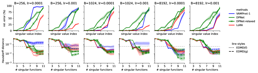
Figure 1: Summary of the noisy logistic map experiment. The first row reports relative error in singular values, and the second row the directed Hausdorff distance of the estimated eigenvalues to the three most dominant underlying eigenvalues. The shaded area indicates $\pm 0.5$ standard deviation.

Example 2. Ordered MNIST. We considered the ordered MNIST example, a synthetic experiment setup which was first considered in (Kostic et al., 2022): given an MNIST image $\mathbf{x}_{t}$ with digit $y_{t}\in\{0,\ldots,4\}$, $\mathbf{x}_{t+1}$ is drawn at random from the MNIST images of digit $y_{t+1}=(y_{t}+1\mod 5)$. While this process is not time-reversible, the process is obviously normal. We tested the same set of methods as before, additionally with sequentially and jointly nested version of LoRA. We trained singular basis parameterized by convolutional neural networks with 100 epochs using 10 random seeds.

We evaluated the multistep prediction performance, by computing (1) the accuracy using an oracle classifier similar to (Kostic et al., 2024a), and (2) root mean squared error (RMSE) of the prediction evaluated on the test data. The multistep prediction performed with EDMD$(\mathbf{g})$ is reported in the first row of Figure 2. We first note that, unlike the catastrophic failure reported in Kostic et al. (2024a), our VAMPnet-1 prediction is reasonably good in terms of both metrics. We highlight that LoRA and its variants consistently outperform the other methods, exhibiting robust RMSE performance over a range of prediction steps $t\in\{-15,\ldots,15\}$. Notably, the nesting techniques helped improve the RMSE performance, especially the joint nesting worked best in this case.

In the second row, we showed the performance of different prediction methods with the basis learned with LoRA_jnt. We note that the quality is very close to each other, and CCA+LoRA prediction seems to follow the trend of EDMD($\mathbf{f}$) for forward prediction and EDMD($\mathbf{g}$) for backward prediction. We also remark that the prediction quality with CCA+LoRA when $t=1$ is particularly bad, which we conjecture to be caused by the absence of the action of Koopman matrices; see Eq. (6) and Eq. (7).

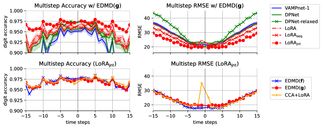
Figure 2: Summary of the ordered MNIST experiment. The shaded area indicates $\pm$standard deviation.

Example 3. Langevin Dynamics. We also tested the performance of LoRA_seq to learn the eigenfunctions of a 1D Langevin dynamics, which is a continuous-time, time-reversible process, where the experiment setup is identical to (Kostic et al., 2024a) and deferred to Appendix. We trained a 3-layer MLP with 128 hidden units using LoRA_seq with $k=10$, employing the Adam optimizer with a learning rate of $10^{-3}$ and a batch size of 128. We report the first eight eigenfunctions and the convergence behavior of the estimated eigenvalues, without any postprocessing other than normalization and sign alignment. We also implemented the DPNet objective $\tilde{\mathcal{L}}_{\mathsf{dp}}^{(\gamma)}(\mathbf{f})$ following the recommended configuration in (Kostic et al., 2024a), but we were unable to obtain successful results. This example demonstrates the effectiveness of the LoRA objective in capturing the generator of continuous-time dynamics.

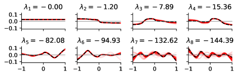
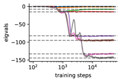
Figure 3: Visualization of the eigenfunctions of the 1D Langevin dynamics, learned by LoRA_seq. In the first panel, the learned eigenfunctions across training iterations are overlaid, with earlier iterations displayed with higher transparency (red). The dashed lines indicate the true eigenfunctions.

Example 4. Chignolin Molecular Dynamics.

We used on the 300 K Chignolin (GYDPETGTWG) dataset from Marshall et al. (2024). This dataset consists of approximately 300,000 snapshots sampled at 100 ps intervals from 34 trajectories grouped by their initial state (folded or unfolded). For training and testing, we sampled 13 and 4 trajectories from each group, respectively, across five random splits. We adopted the SchNet-based architecture and hyperparameters from Kostic et al. (2024a), doubling the batch size to fit our available GPU memory. As reported, both VAMPnet and DPNet diverge during training, leaving DPNet-relaxed as the only converged baseline for our comparisons. To further evaluate the effect of centering, we also introduce an additional baseline, DPNet-relaxed+Cntr, where “Cntr” denotes a centered variant with a fixed constant mode set to $1$. This mirrors the approach used in the LoRA variants (see Section 2.3).

The core objective of this study is to accurately estimate the physically meaningful transition-path time ($\tau_{tp}$) using the learned models. The standard reference for this value is $\tau_{tp}=40_{\pm 10}$ ns, reported for the stabilized variant CLN025 (YDPETGTWY) simulated at 340 K Lindorff-Larsen et al. (2011). Although our experimental setup differs in temperature and amino acids at both ends, these variations are expected to have a minimal impact on $\tau_{tp}$ (see Appendix for details). Therefore, this reference value serves as a valid benchmark for validating the physical accuracy of our models.

Table 2: Test VAMP-2 scores on the 300 K Chignolin dataset Marshall et al. (2024). Algorithms marked with $\dagger$ diverged during training and are therefore omitted. Scores are the mean of five runs with their standard deviation.

Algorithm	Unfolded Init	Folded Init
VAMPnet-1&2†	N/A	N/A
DPNet†	N/A	N/A
DPNet-relaxed	6.25±0.63	4.26±0.76
DPNet-relaxed+Cntr	6.34±0.51	4.26±0.63
LoRA	$10.30_{\pm 1.52}$	$\mathbf{7.34}_{\pm 1.49}$
LoRAjnt	$10.03_{\pm 1.28}$	$6.75_{\pm 1.67}$
LoRAseq	$\mathbf{10.92}_{\pm 1.60}$	$7.04_{\pm 1.66}$

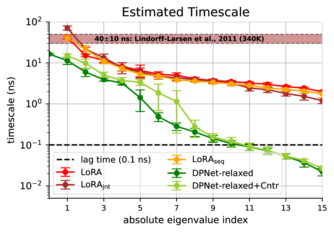
Figure 4: Relaxation time scales on Chignolin. The longest time scale predicted by LoRA and LoRA_seq matches the reference value reported in (Lindorff-Larsen et al., 2011) for the 340 K dataset.

Before analyzing $\tau_{tp}$, we first evaluated the overall quality of the learned kinetic models by measuring the VAMP-2 score on the test data. As shown in Table 2, all LoRA variants achive higher scores than DPNet-relaxed. This suggests that LoRA-based approaches more accurately capture the slow dynamics of the molecular system.

Having confirmed the high performance of our models via the VAMP-2 score, we proceeded to calculate the key physical quantity, the relaxation time, through an eigenvalue analysis on the CCA-aligned singular functions. Each non-trivial eigenvalue $\lambda$ is converted to a time scale using the formula $\tau=-0.1/\log|\lambda|$ ns. Figure 4 shows these results. DPNet-relaxed ($16.5_{\pm 0.6}$ ns) and its centering variant, DPNet-relaxed+Cntr ($15.0_{\pm 1.6}$ ns), significantly underestimate the dominant slow timescale while LoRA_jnt overestimating it at $71.3_{\pm 8.6}$ ns. We also note that the original DPNet work Kostic et al. (2024a) reported similar values to what we derived. In contrast, LoRA and LoRA_seq predict timescales of $42.4_{\pm 4.5}$ ns and $41.2_{\pm 6.6}$ ns, respectively, with both values falling squarely within the reference range of $40_{\pm 10}$ ns. This outcome shows that our proposed methods achieve high statistical scores while also accurately estimating a key physical timescale.

5 Concluding Remarks

The evolution of linear-algebra tools for Koopman analysis, such as DMD, extended DMD, kernel DMD, VAMPnet, and DPNet, mirrors that of CCA and its kernel and maximal-correlation variants. Leveraging recent advances in learning singular functions, we present a new method and a unified learning/inference framework that avoid unstable decompositions and train efficiently with standard mini-batch gradients. Across diverse benchmarks, LoRA variants deliver superior singular subspaces, eigenfunctions, long-horizon forecasts, and scalability, establishing a practical, reliable path for data-driven modeling of complex dynamics. Further gains are expected as deep learning methods and hardware continue to improve.

Limitations. Future work should address the current scarcity of neural architectural search methods and deep learning theory for learning stochastic dynamical systems. Further investigation into LoRA’s specific influence on deep learning optimization is also warranted.

Appendix A Related Work

In this section, we discuss some related work to better contextualize our contribution.

Deep Learning Approaches for Koopman Operator Estimation. Deep learning models are increasingly being integrated into the Koopman theory framework to enable the learning of complex system dynamics by leveraging the expressive power of neural networks. One of the earliest examples is Koopman Autoencoders (KAEs) for forecasting sequential data Williams et al. [2015], Takeishi et al. [2017], Lusch et al. [2018], Azencot et al. [2020]. The KAE approach in general aims to learn a latent embedding and a global, time-invariant linear operator, guided by reconstruction and latent-space constraints. While these methods laid important groundwork, more recent developments Mardt et al. [2018], Kostic et al. [2023, 2024a] have demonstrated superior performance. Consequently, our experimental comparisons concentrate on these more advanced techniques.

Recently, various deep learning architectures for learning Koopman operator have been proposed to handle complex real-world environments, such as non-stationarity in time series data. For example, Koopa Liu et al. [2023] introduced Fourier filters for disentanglement and distinct Koopman predictors for time-variant and invariant components. Another example is Koopman Neural Forecaster Wang et al. [2023], which utilizes predefined measurement functions, a transformer-based local operator, and a feedback loop. We remark, however, that while these methods demonstrate impressive empirical results on some datasets, they primarily prioritize forecasting accuracy rather than the eigenanalysis essential for understanding the underlying system and achieving robust prediction, an objective central to the Koopman analysis framework. In this paper, we focus on the core Koopman framework. Extending our Koopman learning approach to incorporate forecasting capabilities presents an exciting direction for future work.

On Minimizing Low-Rank Approximation Error. Our learning technique closely follows the low-rank-approximation-based framework in [Ryu et al., 2024], including the sequential nesting technique. Ryu et al. [2024] proposed the NestedLoRA framework as a generic tool to perform SVD of a general compact operator using neural networks. While they also considered decomposing the density ratio $\frac{p(\mathbf{y}|\mathbf{x})}{p(\mathbf{y})}$, which they call the canonical dependence kernel (CDK), as a special case, they did not explicitly consider its application to dynamical systems. In general, minimization of the low-rank-approximation error has gained more attention as a more efficient variational framework to characterize the top-$L$ singular subspaces of a given matrix or operator, compared to the common Rayleigh quotient maximization framework and its variants.

During the course of our independent study, we identified an unpublished objective named EYMLoss in the GitHub repository of Kostic et al. [2024a], which effectively corresponds to the LoRA loss investigated in this work; see https://github.com/Machine-Learning-Dynamical-Systems/kooplearn/blob/ca71864469576b39621e4d4e93c0439682166d1e/kooplearn/nn/losses.py#L79C7-L79C14. The associated commit message indicates that the authors were unable to obtain satisfactory results with this formulation. We attribute this failure to a subtle but critical oversight in handling the constant modes. Recall that a Koopman operator, as a special case of CDK operators, admits constant functions as its leading singular functions. In our implementation, we explicitly account for this structure by prepending constant components (i.e., appending 1’s) to the outputs of both the encoder and the lagged encoder. This ensures that the constant modes are appropriately represented and preserved throughout training and inference. In contrast, EYMLoss incorporates the constant modes by projecting out their contribution from the observables. Specifically, it replaces $\mathbf{f}(\mathbf{x})$ with $\mathbf{f}(\mathbf{x})-\mathbb{E}_{\rho_{0}(\mathbf{x})}[\mathbf{f}(\mathbf{x})]$ in the LoRA loss, where the expectation is approximated empirically using minibatch samples. This approach implicitly enforces orthogonality to constant modes by requiring the learned singular functions to be zero-mean with respect to the data distribution. While this treatment is valid in principle, it necessitates that the encoded features remain centered not only during training but also at inference time. Moreover, the constant singular functions must be explicitly included in the final model representation. These additional steps do not appear to have been fully implemented in the kooplearn codebase, which may have contributed to the method’s lack of empirical success.

On Nesting Techniques. The sequential nesting technique in [Ryu et al., 2024] is a function-space version of the triangularized orthogonalization-free method proposed in [Gao et al., 2022]. The joint nesting technique was first proposed specifically for CDK by Xu and Zheng [2024], and later extended as a generic tool by Ryu et al. [2024]. For a more discussion on the history of nesting, we refer to [Ryu et al., 2024].

Appendix B Variational Principles for VAMPnet and DPNet

In this section, we overview the principles behind VAMPnet and DPNet.

B.1 VAMPnet

VAMPnet Wu and Noé [2020], Mardt et al. [2018] is based on the following trace-maximization-type characterization of the top-$k$ singular subspaces.

Theorem B.1.

Let $\mathpzc{T}\colon L_{\rho_{y}}^{2}(\mathcal{Y})\to L_{\rho_{x}}^{2}(\mathcal{X})$ be a compact operator with singular triplets $\{(\sigma_{i},\phi_{i}(\cdot),\psi_{i}(\cdot))\}_{i=1}^{\infty}$, i.e., $(\mathpzc{T}\psi_{i})(x)=\sigma_{i}\phi_{i}(x)$, $(\mathpzc{T}^{*}\phi_{i})(y)=\sigma_{i}\psi_{i}(y)$, and $\sigma_{1}\geq\sigma_{2}\geq\ldots\geq 0$. Then, for any fixed $r=1,2,\ldots$, the optimizers of the following optimization problem

$$\max_{\{(f_{i},g_{i})\}_{i=1}^{k}\subset L_{\rho_{x}}^{2}(\mathcal{X})\times L_{\rho_{y}}^{2}(\mathcal{Y})} ~~~\sum_{i=1}^{k}\langle f_{i},\mathpzc{T}g_{i}\rangle_{\rho_{x}}^{r}$$

subject to $$~~~\mathsf{M}_{\rho_{x}}[\mathbf{f}]=\mathsf{M}_{\rho_{y}}[\mathbf{g}]=\mathsf{I}_{k}$$ (10)

characterize the top-$k$ singular functions of $\mathpzc{T}$ up to an orthogonal transformation.

We refer an interested reader to the proof in [Wu and Noé, 2020]. For the particular case of $\mathpzc{T}$ being a Koopman operator $\mathpzc{K}\colon L_{\rho_{1}}^{2}(\mathcal{X})\to L_{\rho_{0}}^{2}(\mathcal{X})$, Wu and Noé [2020] named the objective

$$\mathcal{R}_{r}[\mathbf{f},\mathbf{g}]\triangleq\sum_{i=1}^{k}\langle f_{i},\mathpzc{K}g_{i}\rangle_{\rho_{0}}^{r}$$ (11)

as the VAMP-$r$ score of $\mathbf{f}$ and $\mathbf{g}$. It is noted that VAMP-1 score is identical to the objective of deep CCA [Andrew et al., 2013]. Wu and Noé [2020], Mardt et al. [2018] advocated the use of VAMP-2 score, based on its relation to the $L_{2}$-approximation error.

In the original VAMP framework [Wu and Noé, 2020, Mardt et al., 2018], neural networks are not directly trained by the VAMP-$r$ score. Instead, they considered a two-stage procedure as follows:

• Basis learning: They parameterize the singular functions as

  $$\mathbf{f}_{\mathsf{U},\theta}(\mathbf{x})\triangleq\mathsf{U}^{\intercal}\mathbf{f}_{\theta}(\mathbf{x}),$$

  $$\mathbf{g}_{\mathsf{V},\theta}(\mathbf{x}^{\prime})\triangleq\mathsf{V}^{\intercal}\mathbf{g}_{\theta}(\mathbf{x}^{\prime}),$$

  where $\mathbf{f}_{\theta}(\mathbf{x})\triangleq(f_{\theta,1}(\mathbf{x}),\ldots,f_{\theta,k_{0}}(\mathbf{x}))^{\intercal}\in\mathbb{R}^{k_{0}}$ and $\mathbf{g}_{\theta}(\mathbf{x}^{\prime})\triangleq(g_{\theta,1}(\mathbf{x}^{\prime}),\ldots,g_{\theta,k_{1}}(\mathbf{x}^{\prime}))^{\intercal}\in\mathbb{R}^{k_{1}}$ denote some basis functions, which in the trainable basis case is typically parameterized by neural networks, and $\mathsf{U}\in\mathbb{R}^{k_{0}\times k}$ and $\mathsf{V}\in\mathbb{R}^{k_{1}\times k}$ denote the projection matrix to further express the singular functions using the given basis. Since the jointly optimizing over all $\theta,\mathsf{U},\mathsf{V}$ is not practical, to train $\mathbf{f}_{\theta}$ and $\mathbf{g}_{\theta}$, they plug-in $\mathbf{f}_{\mathsf{U},\theta}(\mathbf{x})$ and $\mathbf{g}_{\mathsf{V},\theta}(\mathbf{x}^{\prime})$ into Eq. (10), and consider the best $\mathsf{U}$ and $\mathsf{V}$ by solving the partial maximization problem, i.e.,

  $$\max_{\mathsf{U},\mathsf{V}}\mathcal{R}_{r}(\bm{\phi},\bm{\psi})=\Bigl{\|}(\mathsf{M}_{\rho_{0}}[\mathbf{f}])^{-\frac{1}{2}}\mathsf{T}[\mathbf{f},\mathbf{g}](\mathsf{M}_{\rho_{1}}[\mathbf{g}])^{-\frac{1}{2}}\Bigr{\|}_{r}^{r}.$$

  Here, $\|\cdot\|_{r}$ denotes the Schatten $r$-norm. This objective is what we call the (maximal) VAMP-$r$ score in our paper, which is the objective in the VAMP framework that trains the trainable basis functions.

• Inference: Once $\mathbf{f}_{\theta}$ and $\mathbf{g}_{\theta}$ are trained, Eq. (10) become an optimization problem over $\mathsf{U}$ and $\mathsf{V}$:

  $$\max_{\mathsf{U},\mathsf{V}}~ ~\mathcal{R}_{r}(\mathsf{U},\mathsf{V})$$

  subject to $$~\mathsf{U}^{\intercal}\mathsf{M}_{\rho_{0}}[\mathbf{f}]\mathsf{U}=I$$

  $$~\mathsf{V}^{\intercal}\mathsf{M}_{\rho_{1}}[\mathbf{g}]\mathsf{V}=I,$$

  where

  $$\mathcal{R}_{r}(\mathsf{U},\mathsf{V})\triangleq\sum_{i=1}^{k}(\mathbf{u}_{i}^{\intercal}\mathsf{T}[\mathbf{f},\mathbf{g}]\mathbf{v}_{i})^{r}.$$

  Wu and Noé [2020] proposed to solve this using the (linear) CCA algorithm [Hotelling, 1936], and calling the final algorithm feature TCCA. To avoid the degeneracy, basis functions need to be whitened. Strictly speaking, however, the feature TCCA algorithm has nothing to do with the optimization problem. We note that our CCA+LoRA approach is built upon this inference method in the VAMP framework.

Let $\hat{\sigma}_{1},\ldots,\hat{\sigma}_{k}$ denote the top-$k$ singular values of the approximate Koopman matrix $\hat{\mathsf{K}}\triangleq(\mathsf{M}_{\rho_{0}}[\mathbf{f}])^{-\frac{1}{2}}\mathsf{T}[\mathbf{f},\mathbf{g}](\mathsf{M}_{\rho_{1}}[\mathbf{g}])^{-\frac{1}{2}}$. After CCA, we can consider the rank-$k$ approximation of the underlying Koopman operator $\mathpzc{K}$ as we considered in our Approach 1 in Section 3.2. If we call the $\hat{\mathpzc{K}}$ denote the corresponding approximate operator, Wu and Noé [2020] called the (shifted and negated) approximation error in the Hilbert–Schmidt norm

$$\mathcal{R}_{\mathrm{E}}\triangleq\|\mathpzc{K}\|_{\mathrm{HS}}^{2}-\Bigl{\|}\hat{\mathpzc{K}}-\mathpzc{K}\Bigr{\|}_{\mathrm{HS}}^{2}$$

the VAMP-E score. While this looks essentially identical to the low-rank approximation error we consider in this paper, Wu and Noé [2020] and Mardt et al. [2018] used this metric only for evaluation, but not considered for training.

B.2 DPNet

As introduced in the main text, the DPNet objective is given as

$$\mathcal{L}_{\mathsf{dp}}^{(\gamma)}(\mathbf{f},\mathbf{g})\triangleq-\Bigl{\|}(\mathsf{M}_{\rho_{0}}[\mathbf{f}])^{-\frac{1}{2}}\mathsf{T}[\mathbf{f},\mathbf{g}](\mathsf{M}_{\rho_{1}}[\mathbf{g}])^{-\frac{1}{2}}\Bigr{\|}_{\mathrm{F}}^{2}+\gamma(\mathcal{R}(\mathsf{M}_{\rho_{0}}[\mathbf{f}])+\mathcal{R}(\mathsf{M}_{\rho_{1}}[\mathbf{g}])).$$

Here, the metric distortion loss $\mathcal{R}\colon\mathbb{S}_{+}^{L}\to\mathbb{R}_{+}$ is defined as $\mathcal{R}(\mathsf{M})\triangleq\operatorname{tr}(\mathsf{M}^{2}-\mathsf{M}-\ln\mathsf{M})$ for $\mathsf{M}\succeq 0$. If $\gamma=0$ and $\mathsf{M}_{\rho_{0}}[\mathbf{f}]$ and $\mathsf{M}_{\rho_{1}}[\mathbf{g}]$ are nonsingular, the objective becomes equivalent to the VAMP-2 score.

To detour the potential numerical instability in the first term of the DPNet objective, which is essentially the VAMP-2 objective, Kostic et al. [2024a] further proposed a relaxed objective

$$\mathcal{L}_{\mathsf{dpr}}^{(\gamma)}(\mathbf{f},\mathbf{g})\triangleq-\frac{\|\mathsf{T}[\mathbf{f},\mathbf{g}]\|_{\mathrm{F}}^{2}}{\|\mathsf{M}_{\rho_{0}}[\mathbf{f}]\|_{\mathrm{op}}\|\mathsf{M}_{\rho_{1}}[\mathbf{g}]\|_{\mathrm{op}}}+\gamma(\mathcal{R}(\mathsf{M}_{\rho_{0}}[\mathbf{f}])+\mathcal{R}(\mathsf{M}_{\rho_{1}}[\mathbf{g}])).$$

Kostic et al. [2024a] proved the following statement:

Theorem B.2 (Consistency of DPNet objectives).

Let $\gamma\geq 0$. If $\mathpzc{T}$ is compact,

$$\mathcal{L}_{\mathsf{dpr}}^{(\gamma)}(\mathbf{f},\mathbf{g})\geq\mathcal{L}_{\mathsf{dp}}^{(\gamma)}(\mathbf{f},\mathbf{g})\geq-\sum_{i=1}^{k}\sigma_{i}(\mathpzc{T})^{2}.$$

The equalities are attained when $\mathbf{f}(\mathbf{x})$ and $\mathbf{g}(\mathbf{y})$ are the top-$k$ singular functions of $\mathpzc{T}$. If $\mathpzc{T}$ is Hilbert–Schmidt and $\sigma_{L}(\mathpzc{T})>\sigma_{k+1}(\mathpzc{T})$ and $\gamma>0$, the equalities are attained only if $\mathbf{f}(\mathbf{x})$ and $\mathbf{g}(\mathbf{y})$ are orthogonal rotations of top-$k$ singular functions.

Appendix C Special Case of Finite-Rank Koopman Operator

If a given operator is of finite rank, we can analyze the operator using finite-dimensional matrices of the same dimension. We can develop a computational procedure for SVD and eigenanalysis under the finite rank assumption, and apply the tools once we approximate the target operator using a low rank expansion. Some of the results established in this section are used later when (numerically) computing the ground truth characteristics of the noisy logistic map; see Appendix G.1.

Suppose that the Koopman operator $\mathpzc{K}\colon L_{\rho_{1}}^{2}(\mathcal{X})\to L_{\rho_{0}}^{2}(\mathcal{X})$ of our interest is of finite rank. Specifically, the corresponding kernel can be expressed in the following factorized form:

$$k(\mathbf{x},\mathbf{x}^{\prime})=\frac{p(\mathbf{x}^{\prime}|\mathbf{x})}{\rho_{1}(\mathbf{x}^{\prime})}=\bm{\alpha}(\mathbf{x})^{\intercal}\bm{\beta}(\mathbf{x}^{\prime})=\sum_{i=1}^{r}\alpha_{i}(\mathbf{x}){\beta}_{i}(\mathbf{x}^{\prime}).$$

Due to the separable form, the kernel has a rank at most $r$. We aim to find its SVD as follows:

$$k(\mathbf{x},\mathbf{x}^{\prime})=\sum_{i=1}^{r}\sigma_{i}\phi_{i}(\mathbf{x})\psi_{i}(\mathbf{x}^{\prime}),$$ (12)

where the functions satisfy the orthogonality conditions: $\langle\phi_{i},\phi_{j}\rangle_{\rho_{0}}=\langle\psi_{i},\psi_{j}\rangle_{\rho_{1}}=\delta_{ij}$. The singular values $\sigma_{1}\!=\!1\geq\sigma_{2}\geq\ldots\geq\sigma_{r}\geq 0$. The first singular functions $\phi_{1}$ and $\psi_{1}$, corresponding to the trivial mode $\sigma_{1}=1$, are constant functions.

C.1 Singular Value Decomposition

We can compute the singular value decomposition (SVD) using $\mathsf{M}_{\rho_{0}}[\bm{\alpha}]$ and $\mathsf{M}_{\rho_{1}}[\bm{\beta}]$ as follows.

Theorem C.1.

The SVD of the matrix

$$\mathsf{S}_{\rho_{0},\rho_{1}}^{\mathsf{sqrt}}[\bm{\alpha},\bm{\beta}]\triangleq(\mathsf{M}_{\rho_{0}}[\bm{\alpha}])^{1/2}({\mathsf{M}_{\rho_{1}}[\bm{\beta}]})^{1/2}$$

shares the same spectrum, i.e., there exist orthonormal matrices $\mathsf{U}\in\mathbb{R}^{k\times r}$ and $\mathsf{V}\in\mathbb{R}^{k\times r}$ and $\Sigma=\mathsf{diag}(\sigma_{1},\ldots,\sigma_{r})$ such that

$$\mathsf{S}_{\rho_{0},\rho_{1}}^{\mathsf{sqrt}}[\bm{\alpha},\bm{\beta}]=\mathsf{U}\Sigma\mathsf{V}^{\intercal}=\sum_{i=1}^{r}\sigma_{i}\mathbf{u}_{i}\mathbf{v}_{i}^{\intercal}.$$

The ordered, normalized singular functions of the kernel $k(\mathbf{x},\mathbf{x}^{\prime})$ are given as

$$\bm{\phi}(\mathbf{x}) =\mathsf{U}^{\intercal}(\mathsf{M}_{\rho_{0}}[\bm{\alpha}])^{-1/2}\bm{\alpha}(\mathbf{x}),$$ (13)

$$\bm{\psi}(\mathbf{x}^{\prime}) =\mathsf{V}^{\intercal}(\mathsf{M}_{\rho_{1}}[\bm{\beta}])^{-1/2}\bm{\beta}(\mathbf{x}^{\prime}).$$ (14)

Proof.

First of all, it is easy to check that $\mathsf{M}_{\rho_{0}}[\bm{\phi}]=\mathsf{M}_{\rho_{1}}[\bm{\psi}]=\mathsf{I}$. Next, we can show Eq. (12). To show this,

$$\sum_{i=1}^{r}\sigma_{i}\phi_{i}(\mathbf{x})\psi_{i}(\mathbf{x}^{\prime}) =\bm{\phi}(\mathbf{x})^{\intercal}\Sigma\bm{\psi}(\mathbf{x}^{\prime})$$

$$=(\mathsf{U}^{\intercal}(\mathsf{M}_{\rho_{0}}[\bm{\alpha}])^{-1/2}\bm{\alpha}(\mathbf{x}))^{\intercal}\mathsf{U}^{\intercal}\mathsf{S}_{\rho_{0},\rho_{1}}^{\mathsf{sqrt}}[\bm{\alpha},\bm{\beta}]\mathsf{V}(\mathsf{V}^{\intercal}(\mathsf{M}_{\rho_{1}}[\bm{\beta}])^{-1/2}\bm{\beta}(\mathbf{x}^{\prime}))$$

$$=\bm{\alpha}(\mathbf{x})^{\intercal}(\mathsf{M}_{\rho_{0}}[\bm{\alpha}])^{-1/2}((\mathsf{M}_{\rho_{0}}[\bm{\alpha}])^{1/2}(\mathsf{M}_{\rho_{1}}[\bm{\beta}])^{1/2})(\mathsf{M}_{\rho_{1}}[\bm{\beta}])^{-1/2}\bm{\beta}(\mathbf{x}^{\prime})$$

$$=\bm{\alpha}(\mathbf{x})^{\intercal}\bm{\beta}(\mathbf{x}^{\prime})$$

$$=k(\mathbf{x},\mathbf{x}^{\prime}).$$

To show $(\mathpzc{K}\phi_{i})(\mathbf{x}^{\prime})=\sigma_{i}\psi_{i}(\mathbf{x}^{\prime})$, consider

$$(\mathpzc{K}\phi_{i})(\mathbf{x}^{\prime}) \triangleq\int k(\mathbf{x},\mathbf{x}^{\prime})\phi_{i}(\mathbf{x})\rho_{0}(\mathbf{x})dx$$

$$=\bm{\beta}(\mathbf{x}^{\prime})^{\intercal}\int\bm{\alpha}(\mathbf{x})(\mathbf{u}_{i}^{\intercal}(\mathsf{M}_{\rho_{0}}[\bm{\alpha}])^{-1/2}\bm{\alpha}(\mathbf{x}))\rho_{0}(\mathbf{x})dx$$

$$=\bm{\beta}(\mathbf{x}^{\prime})^{\intercal}\int\bm{\alpha}(\mathbf{x})\bm{\alpha}(\mathbf{x})^{\intercal}\rho_{0}(\mathbf{x})dx(\mathsf{M}_{\rho_{0}}[\bm{\alpha}])^{-1/2}\mathbf{u}_{i}$$

$$=\bm{\beta}(\mathbf{x}^{\prime})^{\intercal}(\mathsf{M}_{\rho_{0}}[\bm{\alpha}])^{1/2}\mathbf{u}_{i}$$

$$=\bm{\beta}(\mathbf{x}^{\prime})^{\intercal}({\mathsf{M}_{\rho_{1}}[\bm{\beta}]})^{-1/2}(\mathsf{S}_{\rho_{0},\rho_{1}}^{\mathsf{sqrt}}[\bm{\alpha},\bm{\beta}])^{\intercal}\mathbf{u}_{i}$$

$$=\sigma_{i}\bm{\beta}(\mathbf{x}^{\prime})^{\intercal}({\mathsf{M}_{\rho_{1}}[\bm{\beta}]})^{-1/2}\mathbf{v}_{i}$$

$$=\sigma_{i}\psi_{i}(\mathbf{x}^{\prime}).$$

We can show $(\mathpzc{K}^{*}\psi_{i})(\mathbf{x})=\sigma_{i}\phi_{i}(\mathbf{x})$ by the same reasoning. ∎

C.2 Eigen-analysis

We can compute the eigenvalues and eigenfunctions of the kernel by eigen-analyze the matrices $\mathsf{M}_{\rho_{1}}[\bm{\beta},\bm{\alpha}]$ and $\mathsf{M}_{\rho_{0}}[\bm{\beta},\bm{\alpha}]$.

Theorem C.2.

Let $\mathbf{w}\in\mathbb{C}^{k}$ be a right eigenvector of $\mathsf{M}_{\rho_{1}}[\bm{\beta},\bm{\alpha}]$ with eigenvalue $\lambda\in\mathbb{C}$, i.e., $\mathsf{M}_{\rho_{1}}[\bm{\beta},\bm{\alpha}]\mathbf{w}=\lambda\mathbf{w}$. If we define $\eta(\mathbf{x}^{\prime})\triangleq\mathbf{w}^{\intercal}\bm{\alpha}(\mathbf{x}^{\prime})$, then $\eta$ is a right eigenfunction of $\mathpzc{K}$ with eigenvalue $\lambda$, i.e., $\mathpzc{K}\eta=\lambda\eta$.

Proof.

Since $k(\mathbf{x},\mathbf{x}^{\prime})=\bm{\alpha}(\mathbf{x})^{\intercal}\bm{\beta}(\mathbf{x}^{\prime})$, we have

$$(\mathpzc{K}\eta)(\mathbf{x}) =\int k(\mathbf{x},\mathbf{x}^{\prime})\eta(\mathbf{x}^{\prime})\rho_{1}(\mathbf{x}^{\prime})d\mathbf{x}^{\prime}$$

$$=\bm{\alpha}(\mathbf{x})^{\intercal}\int\bm{\beta}(\mathbf{x}^{\prime})\bm{\alpha}(\mathbf{x}^{\prime})^{\intercal}\mathbf{w}\rho_{1}(\mathbf{x}^{\prime})d\mathbf{x}^{\prime}$$

$$=\bm{\alpha}(\mathbf{x})^{\intercal}\mathsf{M}_{\rho_{1}}[\bm{\beta},\bm{\alpha}]\mathbf{w}$$

$$=\lambda\bm{\alpha}(\mathbf{x})^{\intercal}\mathbf{w}$$

$$=\lambda\eta(\mathbf{x}).\qed$$

Theorem C.3.

Let $\mathbf{z}\in\mathbb{C}^{k}$ be a left eigenvector of $\mathsf{M}_{\rho_{0}}[\bm{\beta},\bm{\alpha}]$ with eigenvalue $\lambda\in\mathbb{C}$, i.e., $\mathbf{z}^{*}\mathsf{M}_{\rho_{0}}[\bm{\beta},\bm{\alpha}]=\lambda\mathbf{z}^{*}$. If we define $\zeta(\mathbf{x}^{\prime})\triangleq\mathbf{z}^{\intercal}\bm{\beta}(\mathbf{x}^{\prime})$, then $\zeta$ is a left eigenfunction of $\mathpzc{K}$ with eigenvalue $\lambda$, i.e., $\mathpzc{K}^{*}\zeta=\overline{\lambda}\zeta$.

Proof.

We have

$$(\mathpzc{K}^{*}\zeta)(\mathbf{x}) =\int k(\mathbf{x},\mathbf{x}^{\prime})\zeta(\mathbf{x})\rho_{0}(\mathbf{x})d\mathbf{x}$$

$$=\bm{\beta}(\mathbf{x}^{\prime})^{\intercal}\int\bm{\alpha}(\mathbf{x})\bm{\beta}(\mathbf{x})^{\intercal}\mathbf{z}\rho_{0}(\mathbf{x})d\mathbf{x}$$

$$=\bm{\beta}(\mathbf{x}^{\prime})^{\intercal}(\mathsf{M}_{\rho_{0}}[\bm{\beta},\bm{\alpha}])^{\intercal}\mathbf{z}$$

$$=\overline{\lambda}\bm{\beta}(\mathbf{x}^{\prime})^{\intercal}\mathbf{z}$$

$$=\overline{\lambda}\zeta(\mathbf{x}^{\prime}).\qed$$

Interestingly, this implies that spectrum of $\mathsf{M}_{\rho_{1}}[\bm{\beta},\bm{\alpha}]$ and $\mathsf{M}_{\rho_{0}}[\bm{\beta},\bm{\alpha}]$ must be identical.

Moreover, if $\mathbf{y}_{o}$ denotes the Perron–Frobenius eigenvector of $\mathsf{M}_{\rho_{0}}[\bm{\beta},\bm{\alpha}]$ (i.e., the left eigenvector with eigenvalue 1), then $g_{o}(\mathbf{x})\triangleq\mathbf{y}_{o}^{\intercal}\bm{\beta}(\mathbf{x})$ is the stationary distribution.

Appendix D Extended DMD and Multi-Step Prediction

In this section, we illustrate the extended DMD procedure [Williams et al., 2014] using basic ideas as elementary as linear regression. Suppose that we are given top-$k$ left and right singular functions $\mathbf{f}(\cdot)$ (encoder) and $\mathbf{g}(\cdot)$ (lagged encoder), respectively. If $h\in\mathsf{span}(\mathbf{f})\triangleq\mathsf{span}\{f_{1},\ldots,f_{k}\}$, then there exists some $\mathbf{z}\in\mathbb{R}^{k}$ such that $h(\mathbf{x})=\mathbf{z}^{\intercal}\mathbf{f}(\mathbf{x})$. Then, we denote by $\mathpzc{K}_{~\mathbf{f}}$ the restriction of the Koopman operator onto the span, which acts on $h$ as

$$(\mathpzc{K}_{~\mathbf{f}}h)(\mathbf{x})=\mathbf{f}(\mathbf{x})^{\intercal}\mathsf{K}_{\mathbf{f}}\mathbf{z}$$

for some $\mathsf{K}_{\mathbf{f}}\in\mathbb{R}^{k\times k}$. With finite data, there are two issues in this picture: (1) How can we compute $\mathsf{K}_{\mathbf{f}}$ from data? (2) Given $h\in\mathsf{span}(\mathbf{f})$, how can we compute the corresponding $\mathbf{z}\in\mathbb{R}^{k}$?

• For the first question, the extended DMD aims to find the best finite-dimensional approximation of the Koopman operator $\mathpzc{K}$ restricted on $\mathsf{span}(\mathbf{f})$, in the sense that $(\mathpzc{K}\mathbf{f})(\mathbf{x})=\mathbb{E}_{p(\mathbf{x}^{\prime}|\mathbf{x})}[\mathbf{f}(\mathbf{x}^{\prime})]\approx\mathsf{K}\mathbf{f}(\mathbf{x})$. As a natural choice, we can choose the ordinary least square solution that solves $\mathbf{f}(\mathbf{x}^{\prime})=\mathsf{K}\mathbf{f}(\mathbf{x})$ for $(\mathbf{x},\mathbf{x}^{\prime})\sim\rho_{0}(\mathbf{x})p(\mathbf{x}^{\prime}|\mathbf{x})$, where

  $$\hat{\mathsf{K}}_{\mathbf{f}}^{\mathsf{ols}}\triangleq\mathsf{F}^{+}\mathsf{F}^{\prime}=(\mathsf{F}^{\intercal}\mathsf{F})^{-1}\mathsf{F}^{\intercal}\mathsf{F}^{\prime}=(\hat{\mathsf{M}}_{\rho_{0}}[\mathbf{f}])^{-1}\hat{\mathsf{T}}[\mathbf{f}],$$

  where we denote the data matrices by

  $$\mathsf{F}\triangleq[\mathbf{f}(\mathbf{x}_{1})\ldots\mathbf{f}(\mathbf{x}_{N})]^{\intercal}\in\mathbb{R}^{N\times k}\quad\text{and}\quad\mathsf{F}^{\prime}\triangleq[\mathbf{f}(\mathbf{x}_{1}^{\prime})\ldots\mathbf{f}(\mathbf{x}_{N}^{\prime})]^{\intercal}\in\mathbb{R}^{N\times k}.$$

  Note that $\hat{\mathsf{M}}_{\rho_{0}}[\mathbf{f}]$ and $\hat{\mathsf{T}}[\mathbf{f}]$ are the empirical estimates of the second moment matrices $\mathsf{M}_{\rho_{0}}[\mathbf{f}]$ and $\mathsf{T}[\mathbf{f}]$.

• For the second point, we can again view this as a linear regression problem, since

  $$h(\mathbf{x}_{i})=\mathbf{z}^{\intercal}\mathbf{f}(\mathbf{x}_{i})\quad\text{for }i=1,\ldots,N.$$

  Hence, we can define the best $\mathbf{z}$ again as the OLS solution ${\mathbf{z}}_{h}^{\mathsf{ols}}[\mathbf{f}]\triangleq\mathsf{F}^{+}{\mathsf{H}}=(\hat{\mathsf{M}}_{\rho_{0}}[\mathbf{f}])^{-1}\mathsf{F}^{\intercal}{\mathsf{H}}$, where

  $${\mathsf{H}}\triangleq\begin{bmatrix}h(\mathbf{x}_{1}),\ldots,h(\mathbf{x}_{N})\end{bmatrix}^{\intercal}\in\mathbb{R}^{N}.$$

Now, suppose that we already computed $\hat{\mathsf{T}}[\mathbf{f},\mathbf{g}]$ and $\hat{\mathbf{z}}_{h}$ from data. Then, we can approximate the multi-step prediction as

$$\mathbb{E}_{p(\mathbf{x}_{t}|\mathbf{x}_{0})}[h(\mathbf{x}_{t})]\approx\mathbf{f}(\mathbf{x}_{0})^{\intercal}\hat{\mathsf{T}}[\mathbf{f},\mathbf{g}]^{t}\hat{\mathbf{z}}_{h}.$$ (15)

The same logic applies to the subspace spanned by the right singular functions $\psi(\cdot)$.

Appendix E Deferred Technical Statements and Proofs

In this section, we provide a short derivation of the low-rank approximation (LoRA) loss for completeness, and present a learning-theoretic guarantee for the LoRA objective.

E.1 Derivation of Low-Rank Approximation Loss

Proposition E.1.

$$\min_{\mathbf{f},\mathbf{g}}\Bigl{\|}\mathpzc{K}-\sum_{i=1}^{k}f_{i}\otimes g_{i}\Bigr{\|}_{\mathrm{HS}}^{2}=\min_{\mathbf{f},\mathbf{g}}\mathcal{L}_{\mathsf{lora}}(\mathbf{f},\mathbf{g}).$$

Proof of Proposition E.1.

Recall that $\mathcal{L}_{\mathsf{lora}}(\mathbf{f},\mathbf{g})\triangleq-2\operatorname{tr}(\mathsf{T}[\mathbf{f},\mathbf{g}])+\operatorname{tr}(\mathsf{M}_{\rho_{0}}[\mathbf{f}]\mathsf{M}_{\rho_{1}}[\mathbf{g}])$. To prove, first note that

$$\Bigl{\|}\mathpzc{K}-\sum_{i=1}^{k}f_{i}\otimes g_{i}\Bigr{\|}_{\mathrm{HS}}^{2}-\|\mathpzc{K}\|_{\mathrm{HS}}^{2}=-2\sum_{i=1}^{k}\langle f_{i},\mathpzc{K}g_{i}\rangle_{\rho_{0}}+\sum_{i=1}^{k}\sum_{j=1}^{k}\langle f_{i},f_{j}\rangle_{\rho_{0}}\langle g_{i},g_{j}\rangle_{\rho_{1}}.$$

Here, the first term can be rewritten as

$$\sum_{i=1}^{k}\langle f_{i},\mathpzc{K}g_{i}\rangle_{\rho_{0}} =\sum_{i=1}^{k}\mathbb{E}_{\rho_{0}(\mathbf{x})p(\mathbf{x}^{\prime}|\mathbf{x})}[f_{i}(\mathbf{x})g_{i}(\mathbf{x}^{\prime})]$$

$$=\operatorname{tr}\bigl{(}\mathbb{E}_{\rho_{0}(\mathbf{x})p(\mathbf{x}^{\prime}|\mathbf{x})}\bigl{[}\mathbf{f}(\mathbf{x})\mathbf{g}(\mathbf{x}^{\prime})^{\intercal}\bigr{]}\bigr{)}$$

$$=\operatorname{tr}(\mathsf{T}[\mathbf{f},\mathbf{g}]).$$

Likewise, the second term is

$$\sum_{i=1}^{k}\sum_{j=1}^{k}\langle f_{i},f_{j}\rangle_{\rho_{0}}\langle g_{i},g_{j}\rangle_{\rho_{1}} =\operatorname{tr}\bigl{(}\mathbb{E}_{\rho_{0}(\mathbf{x})}\bigl{[}\mathbf{f}(\mathbf{x})\mathbf{f}(\mathbf{x})^{\intercal}\bigr{]}\mathbb{E}_{\rho_{1}(\mathbf{x}^{\prime})}\bigl{[}\mathbf{g}(\mathbf{x}^{\prime})\mathbf{g}(\mathbf{x}^{\prime})^{\intercal}\bigr{]}\bigr{)}$$

$$=\operatorname{tr}(\mathsf{M}_{\rho_{0}}[\mathbf{f}]\mathsf{M}_{\rho_{1}}[\mathbf{g}]).$$

This concludes the proof. ∎

E.2 Statistical Learning Guarantee

We consider empirical estimates of the second moment matrices $\mathsf{T}[\mathbf{f},\mathbf{g}],\mathsf{M}_{\rho_{0}}[\mathbf{f}],\mathsf{M}_{\rho_{1}}[\mathbf{g}]$.

$$\hat{\mathsf{T}}[\mathbf{f},\mathbf{g}] \triangleq\displaystyle\frac{1}{N}\sum_{t=1}^{N}\mathbf{f}(\mathbf{x}_{t})\mathbf{g}(\mathbf{x}_{t}^{\prime})^{\intercal},$$

$$\hat{\mathsf{M}}_{\rho_{0}}[\mathbf{f}] \triangleq\displaystyle\frac{1}{N_{0}}\sum_{i=1}^{N_{0}}\mathbf{f}(\breve{\mathbf{x}}_{i})\mathbf{f}(\breve{\mathbf{x}}_{i})^{\intercal},$$

$$\hat{\mathsf{M}}_{\rho_{1}}[\mathbf{g}] \triangleq\displaystyle\frac{1}{N_{1}}\sum_{j=1}^{N}\mathbf{g}(\breve{\mathbf{x}}_{j}^{\prime})\mathbf{g}(\breve{\mathbf{x}}_{j}^{\prime})^{\intercal}.$$

Here, $(\mathbf{x}_{t},\mathbf{x}_{t}^{\prime})\sim\rho_{0}(\mathbf{x})p(\mathbf{x}^{\prime}|\mathbf{x})$ are i.i.d. samples and $\breve{\mathbf{x}}_{i}\sim\rho_{0}(\mathbf{x})$ and $\breve{\mathbf{x}}_{j}^{\prime}\sim\rho_{1}(\mathbf{x}^{\prime})$ are i.i.d. samples.

Note that, if we follow the common data collection procedure, $\breve{\mathbf{x}}_{i}\sim\rho_{0}(\mathbf{x})$ and $\breve{\mathbf{x}}_{j}^{\prime}\sim\rho_{1}(\mathbf{x}^{\prime})$ are drawn from a single trajectory, and thus the samples $(\breve{\mathbf{x}},\breve{\mathbf{x}}^{\prime})$ cannot be independent. The independence assumption between $\{\breve{\mathbf{x}}_{i}\}$ and $\{\breve{\mathbf{x}}_{j}^{\prime}\}$ are for the sake of simpler analysis. In practice, however, this can be enforced by splitting the set of given independent trajectories into two subsets and compute $\hat{\mathsf{M}}_{\rho_{0}}[\mathbf{f}]$ and $\hat{\mathsf{M}}_{\rho_{1}}[\mathbf{g}]$ with different subsets of samples.

Theorem E.1.

Let $\|\mathbf{f}(\mathbf{x})\|\leq R$ and $\|\mathbf{g}(\mathbf{x}^{\prime})\|\leq R$ almost surely for some $R>0$. Let $\mathsf{V}_{\mathbf{f}}\triangleq\mathbb{E}_{\rho_{0}(\mathbf{x})}[(\mathbf{f}(\mathbf{x})\mathbf{f}(\mathbf{x})^{\intercal}-\mathsf{M}_{\rho_{0}}[\mathbf{f}])^{2}]\in\mathbb{R}^{k\times k}$ and $\mathsf{V}_{\mathbf{g}}\triangleq\mathbb{E}_{\rho_{1}(\mathbf{x}^{\prime})}[(\mathbf{g}(\mathbf{x}^{\prime})\mathbf{g}(\mathbf{x}^{\prime})^{\intercal}-\mathsf{M}_{\rho_{1}}[\mathbf{g}])^{2}]\in\mathbb{R}^{k\times k}$. Then, with probability at least $1-\delta$, we have

$$|\hat{\mathcal{L}}-\mathcal{L}| \leq R^{2}\Biggl{\{}\sqrt{\frac{16}{N}\log\frac{6}{\delta}}+\frac{8}{3N}\log\frac{6}{\delta}$$

$$\qquad\qquad+\sqrt{\frac{2\|\mathsf{V}_{\mathbf{f}}\|_{\mathrm{op}}}{N_{0}}\log\frac{12r(\mathsf{V}_{\mathbf{f}})}{\delta}}+\frac{2R^{2}}{3N_{0}}\log\frac{12r(\mathsf{V}_{\mathbf{f}})}{\delta}$$

$$\qquad\qquad+\sqrt{\frac{2\|\mathsf{V}_{\mathbf{g}}\|_{\mathrm{op}}}{N_{1}}\log\frac{12r(\mathsf{V}_{\mathbf{g}})}{\delta}}+\frac{2R^{2}}{3N_{1}}\log\frac{12r(\mathsf{V}_{\mathbf{g}})}{\delta}\Biggr{\}}.$$

To prove this, we will invoke Bernstein inequalities for bounded random variables and “bounded” self-adjoint matrices:

Lemma E.1 (Bernstein’s inequality [Tropp, 2015, Theorem 1.6.1]).

Let $X_{1},\ldots,X_{n}$ be i.i.d. copies of a random variable $X$ such that $|X|\leq u$ almost surely, $\mathbb{E}[X]=0$, and $\mathbb{E}[X^{2}]\leq\sigma^{2}$. Then, for any $\delta\in(0,1)$, with probability at least $1-\delta$,

$$\Biggl{|}\frac{1}{n}\sum_{i=1}^{n}X_{i}\Biggr{|}\leq\frac{4u}{3n}\log\frac{2}{\delta}+\sqrt{\frac{4\sigma^{2}}{n}\log\frac{2}{\delta}}.$$

Lemma E.2 (Matrix Bernstein inequality with intrinsic dimension [Minsker, 2017], [Tropp, 2015, Theorem 7.7.1]).

Let $\mathsf{A}_{1},\ldots,\mathsf{A}_{n}$ be i.i.d. copies of a random self-adjoint matrix $\mathsf{A}$, which satisfies $\|\mathsf{A}\|_{\mathrm{op}}\leq c$ almost surely, $\mathbb{E}[\mathsf{A}]=0$, and $\mathbb{E}[\mathsf{A}^{2}]=\mathsf{V}\succeq 0$. Let $r(\mathsf{V})\triangleq\frac{\operatorname{tr}(\mathsf{V})}{\|\mathsf{V}\|_{\mathrm{op}}}$ denote the intrinsic dimension of $\mathsf{V}$. Then, for any $\delta\in(0,1)$, with probability at least $1-\delta$,

$$\Biggl{\|}\frac{1}{n}\sum_{i=1}^{n}\mathsf{A}_{i}\Biggr{\|}_{\mathrm{op}}\leq\frac{2c}{3n}\log\frac{4r(\mathsf{V})}{\delta}+\sqrt{\frac{2\|\mathsf{V}\|_{\mathrm{op}}}{n}\log\frac{4r(\mathsf{V})}{\delta}}.$$

We are now ready to prove Theorem E.1.

Proof of Theorem E.1.

Consider

$$|\hat{\mathcal{L}}-\mathcal{L}| =\Bigl{|}\operatorname{tr}(-2\hat{\mathsf{T}}[\mathbf{f},\mathbf{g}]+\hat{\mathsf{M}}_{\rho_{0}}[\mathbf{f}]\hat{\mathsf{M}}_{\rho_{1}}[\mathbf{g}])-\operatorname{tr}(-2\mathsf{T}[\mathbf{f},\mathbf{g}]+\mathsf{M}_{\rho_{0}}[\mathbf{f}]\mathsf{M}_{\rho_{1}}[\mathbf{g}])\Bigr{|}$$

$$\leq 2|\operatorname{tr}(\hat{\mathsf{T}}[\mathbf{f},\mathbf{g}]-\mathsf{T}[\mathbf{f},\mathbf{g}])|+|\operatorname{tr}(\hat{\mathsf{M}}_{\rho_{0}}[\mathbf{f}]\hat{\mathsf{M}}_{\rho_{1}}[\mathbf{g}]-\mathsf{M}_{\rho_{0}}[\mathbf{f}]\mathsf{M}_{\rho_{1}}[\mathbf{g}])|.$$

For the first term $|\operatorname{tr}(\hat{\mathsf{T}}[\mathbf{f},\mathbf{g}]-\mathsf{T}[\mathbf{f},\mathbf{g}])|$, note that

$$\operatorname{tr}(\hat{\mathsf{T}}[\mathbf{f},\mathbf{g}]-\mathsf{T}[\mathbf{f},\mathbf{g}])=\frac{1}{N}\sum_{t=1}^{N}\mathbf{f}(\mathbf{x}_{t})^{\intercal}\mathbf{g}(\mathbf{x}_{t}^{\prime})-\mathbb{E}_{\rho_{0}(\mathbf{x})p(\mathbf{x}^{\prime}|\mathbf{x})}\bigl{[}\mathbf{f}(\mathbf{x})^{\intercal}\mathbf{g}(\mathbf{x}^{\prime})\bigr{]}.$$

Here, we note that

$$|\mathbf{f}(\mathbf{x})^{\intercal}\mathbf{g}(\mathbf{x}^{\prime})| \leq\|\mathbf{f}(\mathbf{x})\|\cdot\|\mathbf{g}(\mathbf{x}^{\prime})\|\leq R^{2},$$

$$(\mathbf{f}(\mathbf{x})^{\intercal}\mathbf{g}(\mathbf{x}^{\prime}))^{2} \leq R^{4}.$$

Hence, we can apply Bernstein’s inequality in Lemma E.1 for $(\mathbf{f}(\mathbf{x}_{t})^{\intercal}\mathbf{g}(\mathbf{x}_{t}^{\prime}))_{t=1}^{N}$ with $u\leftarrow R^{2}$, $\sigma^{2}\leftarrow R^{4}$, and $\delta\leftarrow\delta^{\prime}$, where $\delta^{\prime}$ is to be decided at the end of proof.

Now, we wish to bound $|\operatorname{tr}(\hat{\mathsf{M}}_{\rho_{0}}[\mathbf{f}]\hat{\mathsf{M}}_{\rho_{1}}[\mathbf{g}]-\mathsf{M}_{\rho_{0}}[\mathbf{f}]\mathsf{M}_{\rho_{1}}[\mathbf{g}])|$.

Let $\Delta_{\mathbf{f}}\triangleq\hat{\mathsf{M}}_{\rho_{0}}[\mathbf{f}]-\mathsf{M}_{\rho_{0}}[\mathbf{f}]$ and $\Delta_{\mathbf{g}}\triangleq\hat{\mathsf{M}}_{\rho_{1}}[\mathbf{g}]-\mathsf{M}_{\rho_{1}}[\mathbf{g}]$. Then,

$$|\operatorname{tr}(\hat{\mathsf{M}}_{\rho_{0}}[\mathbf{f}]\hat{\mathsf{M}}_{\rho_{1}}[\mathbf{g}]-\mathsf{M}_{\rho_{0}}[\mathbf{f}]\mathsf{M}_{\rho_{1}}[\mathbf{g}])| =|\operatorname{tr}(\Delta_{\mathbf{f}}\mathsf{M}_{\rho_{1}}[\mathbf{g}]+\hat{\mathsf{M}}_{\rho_{0}}[\mathbf{f}]\Delta_{\mathbf{g}})|$$

$$\leq|\operatorname{tr}(\Delta_{\mathbf{f}}\mathsf{M}_{\rho_{1}}[\mathbf{g}])|+|\operatorname{tr}(\hat{\mathsf{M}}_{\rho_{0}}[\mathbf{f}]\Delta_{\mathbf{g}})|$$

$$\stackrel{{\scriptstyle(a)}}{{\leq}}\|\Delta_{\mathbf{f}}\|_{\rm op}\operatorname{tr}(\mathsf{M}_{\rho_{1}}[\mathbf{g}])+\|\Delta_{\mathbf{g}}\|_{\rm op}\operatorname{tr}(\hat{\mathsf{M}}_{\rho_{0}}[\mathbf{f}])$$

$$=\|\Delta_{\mathbf{f}}\|_{\rm op}\mathbb{E}_{\pi}[\|\mathbf{g}(\mathbf{x}^{\prime})\|^{2}]+\|\Delta_{\mathbf{g}}\|_{\rm op}\frac{1}{N_{1}}\sum_{j=1}^{N_{1}}\|\mathbf{g}(\mathbf{x}_{j}^{\prime})\|^{2}$$

$$\stackrel{{\scriptstyle(b)}}{{\leq}}R^{2}\Bigl{(}\|\Delta_{\mathbf{f}}\|_{\rm op}+\|\Delta_{\mathbf{g}}\|_{\rm op}\Bigr{)}.$$

where $(a)$ follows from the inequality $|\operatorname{tr}(\mathsf{A}\mathsf{B})|\leq\|\mathsf{A}\|_{\mathrm{op}}\operatorname{tr}(\mathsf{B})$ for square matrices $\mathsf{A},\mathsf{B}$ such that $\mathsf{B}\succeq 0$, and $(b)$ from the boundedness assumption, i.e., $\|\mathbf{f}(\mathbf{x})\|\leq R$ and $\|\mathbf{g}(\mathbf{x}^{\prime})\|\leq R$ almost surely. Here, we can apply the matrix Bernstein inequality in Lemma E.2 to bound $\|\Delta_{\mathbf{f}}\|_{\rm op}$ with $\mathsf{A}\leftarrow\mathbf{f}(\mathbf{x})\mathbf{f}(\mathbf{x})^{\intercal}-\mathsf{M}_{\rho_{0}}[\mathbf{f}]$ with $\delta\leftarrow 1-\delta^{\prime}$, and similarly for $\|\Delta_{\mathbf{g}}\|_{\rm op}$.

Finally, by applying the union bound on the Bernstein inequality and two matrix Bernstein inequalities with $\delta^{\prime}=\delta/3$, we can conclude the desired bound. ∎

Appendix F On Implementation

In this section, we explain how we can implement nesting with automatic differentiation and provide a pseudocode in PyTorch [Paszke et al., 2019].

F.1 Implementation of Nesting Techniques

We can implement the sequential nesting by computing the derivative of the following objective using automatic differentiation:

$$\mathcal{L}_{\mathsf{lora}}^{\mathsf{seq}}(\mathbf{f},\mathbf{g})\triangleq-2\operatorname{tr}(\mathsf{M}_{\rho_{0}}^{\mathsf{seq}}[\mathbf{f},\mathpzc{K}\mathbf{g}])+\operatorname{tr}(\mathsf{M}_{\rho_{0}}^{\mathsf{seq}}[\mathbf{f}]\mathsf{M}_{\rho_{1}}^{\mathsf{seq}}[\mathbf{g}]),$$

where we define a partially stop-gradiented second moment matrix

$$\mathsf{M}_{\rho}^{\mathsf{seq}}[\mathbf{f},\mathbf{g}]\triangleq\begin{bmatrix}\langle f_{1},f_{1}\rangle_{\rho}&\langle\mathsf{sg}[f_{1}],f_{2}\rangle_{\rho}&\langle\mathsf{sg}[f_{1}],f_{3}\rangle_{\rho}&\cdots&\langle\mathsf{sg}[f_{1}],f_{k}\rangle_{\rho}\\ \langle f_{2},\mathsf{sg}[f_{1}]\rangle_{\rho}&\langle f_{2},f_{2}\rangle_{\rho}&\langle\mathsf{sg}[f_{2}],f_{3}\rangle_{\rho}&\cdots&\langle\mathsf{sg}[f_{2}],f_{k}\rangle_{\rho}\\ \langle f_{3},\mathsf{sg}[f_{1}]\rangle_{\rho}&\langle f_{3},\mathsf{sg}[f_{2}]\rangle_{\rho}&\langle f_{3},f_{3}\rangle_{\rho}&\cdots&\langle\mathsf{sg}[f_{3}],f_{k}\rangle_{\rho}\\ \vdots&\vdots&\ddots&\vdots\\ \langle f_{k},\mathsf{sg}[f_{1}]\rangle_{\rho}&\langle f_{k},\mathsf{sg}[f_{2}]\rangle_{\rho}&\langle f_{k},\mathsf{sg}[f_{3}]\rangle_{\rho}&\cdots&\langle f_{k},f_{k}\rangle_{\rho}\end{bmatrix}.$$

This can be implemented efficiently with almost no additional computation. We note that the implementation of the sequentially nested LoRA we provide here is a more direct and simpler version than the implementation of NeuralSVD in [Ryu et al., 2024], which implemented the sequential nesting by a custom gradient.

The joint nesting can be also implemented in an efficient manner via the matrix mask, as explained in [Ryu et al., 2024]. Define the matrix mask $\mathsf{P}\in\mathbb{R}^{k\times k}$ as $\mathsf{P}_{ij}=\mathsf{m}_{\max\{i,j\}}$ with $\mathsf{m}_{i}\triangleq\sum_{j=i}^{k}\alpha_{j}$. Then, $\mathcal{L}_{\mathsf{lora}}^{\mathsf{joint}}(\mathbf{f},\mathbf{g};\bm{\alpha})\triangleq\sum_{i=1}^{k}\alpha_{i}\mathcal{L}_{\mathsf{lora}}(\mathbf{f}_{1:i},\mathbf{g}_{1:i})$ Then, we can write

$$\mathcal{L}_{\mathsf{lora}}^{\mathsf{joint}}(\mathbf{f},\mathbf{g};\bm{\alpha})=\sum_{i=1}^{k}\alpha_{i}\mathcal{L}_{\mathsf{lora}}(\mathbf{f}_{1:i},\mathbf{g}_{1:i})=\operatorname{tr}\Bigl{(}\mathsf{P}\odot\Bigl{(}-2\mathsf{M}_{\rho_{0}}[\mathbf{f},\mathpzc{K}\mathbf{g}]+\mathsf{M}_{\rho_{0}}[\mathbf{f}]\mathsf{M}_{\rho_{1}}[\mathbf{g}]\Bigr{)}\Bigr{)}.$$

F.2 Pseudocode for NestedLoRA Loss

Based on the nesting techniques described above, here we provide a simple and efficient PyTorch [Paszke et al., 2019] implementation of the NestedLoRA objective.

⬇

1class NestedLoRALoss:

2 def __init__(

3 self,

4 use_learned_svals=False,

5 nesting=None,

6 n_modes=None,

7 ):

8 self.use_learned_svals = use_learned_svals

9 assert nesting in [None, ’seq’, ’jnt’]

10 self.nesting = nesting

11 if self.nesting == ’jnt’:

12 assert n_modes is not None

13 self.vec_mask, self.mat_mask = get_joint_nesting_masks(

14 weights=np.ones(n_modes) / n_modes,

15 )

16 else:

17 self.vec_mask, self.mat_mask = None, None

18 self.kostic_regularization = kostic_regularization

19

20 def __call__(self, f: torch.Tensor, g: torch.Tensor):

21 # f: [b, k]

22 # g: [b, k]

23

24 if self.nesting == ’jnt’:

25 # \sum_{i=1}^k <f_i, T g_i >

26 corr_term = -2 * (self.vec_mask.to(f.device) * f * g).mean(0).sum()

27 # \sum_{i=1}^k \sum_{j=1}^k <f_i, f_j> <g_i, g_j>

28 # = tr ( cov (f_{1:k}) * cov(g_{1:k}) )

29 M_f = compute_second_moment(f)

30 M_g = compute_second_moment(g)

31 metric_term = (self.mat_mask.to(f.device) * M_f * M_g).sum()

32

33 else:

34 # \sum_{i=1}^k <f_i, T g_i >

35 corr_term = -2 * (f * g).mean(0).sum()

36 # \sum_{i=1}^k \sum_{j=1}^k <f_i, f_j> <g_i, g_j>

37 # = tr ( cov (f_{1:k}) * cov(g_{1:k}) )

38 M_f = compute_second_moment(f, seq_nesting=self.nesting == ’seq’)

39 M_g = compute_second_moment(g, seq_nesting=self.nesting == ’seq’)

40 metric_term = (M_f * M_g).sum()

41

42 return corr_term + metric_term

43

44def compute_second_moment(

45 f: torch.Tensor,

46 g: torch.Tensor = None,

47 seq_nesting: bool = False

48 ) -> torch.Tensor:

49 """

50 compute (optionally sequentially nested) second-moment matrix

51 M_ij = <f_i, g_j>

52 with partial stop-gradient handling when seq_nesting is True.

53

54 args

55 ----

56 f : (n, k) tensor

57 g : (n, k) tensor or None

58 seq_nesting : bool

59 """

60 if g is None:

61 g = f

62 n = f.shape[0]

63 if not seq_nesting:

64 return (f.T @ g) / n

65 else:

66 # partial stop gradient

67 # lower-triangular: <f_i, sg[g_j]> for i > j

68 lower = torch.tril(f.T @ g.detach(), diagonal=-1)

69 # upper-triangular: <sg[f_i], g_j> for i < j

70 upper = torch.triu(f.detach().T @ g, diagonal=+1)

71 # diagonal: <f_i, g_i> (no stop-grad)

72 diag = torch.diag((f * g).sum(dim=0))

73 return (lower + diag + upper) / n

74

75def get_joint_nesting_masks(weights: np.ndarray):

76 vector_mask = list(np.cumsum(list(weights)[::-1])[::-1])

77 vector_mask = torch.tensor(np.array(vector_mask)).float()

78 matrix_mask = torch.minimum(

79 vector_mask.unsqueeze(1), vector_mask.unsqueeze(1).T

80 ).float()

81 return vector_mask, matrix_mask

Appendix G Deferred Details on Experiments

In this section, we provide details for each experiment. See Table 3 for an overview of the benchmark problems from [Kostic et al., 2024a]. Our implementation builds upon the codebase of [Kostic et al., 2024a], the kooplearn package, and the codebase of [Ryu et al., 2024]. We will publicize our code upon acceptance.

Table 3: Overview of the experiments.

Examples	Time	Spectral complexity	Stationarity
noisy logistic map	discrete	non-normal	(nearly) stationary
ordered MNIST	discrete	normal	stationary
1D SDE	continuous	self-adjoint	(nearly) stationary
molecular dynamics	continuous (discretized)	normal	non-stationary

G.1 Noisy Logistic Map

We consider a dynamical system defined as $X_{t+1}=(F(X_{t})+\xi_{t})~{\rm mod}~1$, for $F(x)\triangleq rx(1-x)$ for $x\in\mathcal{X}=[0,1)$ and $\xi_{t}\sim p(\xi)$. Here, $p(\xi)\triangleq C_{N}\cos^{N}(\pi\xi)$ is the order $N$ trigonometric noise over $\xi\in[-0.5,0.5]$ [Ostruszka et al., 2000], where $C_{N}\triangleq\pi/B(\frac{N+1}{2},\frac{1}{2})$ is the (reciprocal) normalization constant. For this simple example, we can write

$$p(x^{\prime}|x)=\sum_{i=0}^{N}\alpha_{i}(x)\breve{\beta}_{i}(x^{\prime}),$$

where

$$\breve{\beta}_{i}(x) \triangleq\sqrt{C_{N}\binom{N}{i}}\cos^{i}(\pi x)\sin^{N-i}(\pi x),$$

$$\alpha_{i}(x) \triangleq\breve{\beta}_{i}(F(x)).$$

Let $\beta_{i}(x^{\prime})\triangleq\frac{\breve{\beta}_{i}(x^{\prime})}{\rho_{1}(x^{\prime})}$ such that we can write $\frac{p(x^{\prime}|x)}{\rho_{1}(x^{\prime})}=\bm{\alpha}(x)^{\intercal}\bm{\beta}(x^{\prime})$.

Computation of Ground-Truth Properties. Since the operator is of finite rank, we can invoke the results in Appendix C. Let

$$\mathsf{M}_{\pi}[\bm{\phi},\bm{\alpha}] \triangleq\mathbb{E}_{\pi}[\bm{\phi}(\mathbf{x})\bm{\alpha}(\mathbf{x})^{\intercal}],$$

$$\mathsf{M}_{\pi}[\bm{\phi},\bm{\beta}] \triangleq\mathbb{E}_{\pi}[\bm{\phi}(\mathbf{x}){\bm{\beta}}(\mathbf{x})^{\intercal}].$$

Note that

$$\mathsf{M}_{\pi}[\bm{\phi},\bm{\alpha}]\mathsf{M}_{\pi}[\bm{\phi},\bm{\beta}]^{\intercal} =\mathbb{E}_{\rho_{0}(\mathbf{x})\rho_{1}(\mathbf{x}^{\prime})}\Bigl{[}\bm{\phi}(\mathbf{x})\bm{\alpha}(\mathbf{x})^{\intercal}{\bm{\beta}}(\mathbf{x}^{\prime})\bm{\phi}(\mathbf{x}^{\prime})^{\intercal}\Bigr{]}$$

$$=\mathbb{E}_{\rho_{0}(\mathbf{x})\rho_{1}(\mathbf{x}^{\prime})}\Bigl{[}\bm{\phi}(\mathbf{x})k(\mathbf{x},\mathbf{x}^{\prime})\bm{\phi}(\mathbf{x}^{\prime})^{\intercal}\Bigr{]}$$

$$=\mathbb{E}_{\rho_{0}(\mathbf{x})p(\mathbf{x}^{\prime}|\mathbf{x})}[\bm{\phi}(\mathbf{x})\bm{\phi}(\mathbf{x}^{\prime})^{\intercal}]=\mathsf{T}[\bm{\phi}].$$

Then we can compute the approximate Koopman matrix as the ordinary least square regression, which is equivalent to the extended DMD:

$$\hat{\mathsf{K}}_{\bm{\phi}}^{\mathsf{ols}}=(\mathsf{M}_{\pi}[\bm{\phi}])^{-1}\mathsf{T}[\bm{\phi}]=(\mathsf{M}_{\pi}[\bm{\phi}])^{-1}\mathsf{M}_{\pi}[\bm{\phi},\bm{\alpha}]\mathsf{M}_{\pi}[\bm{\phi},\bm{\beta}]^{\intercal}.$$

Implementation. We used a multi-layer perceptron (MLP) with hidden units 64-128-64 and leaky ReLU activation. The main text has all the details to reproduce the results.

G.2 Ordered MNIST

Following the setup of [Kostic et al., 2024a], we generated two independent trajectories of length 1000. We used one trajectory for training and the other for evaluation. We used Adam optimizer with learning rate $10^{-3}$, batch size 64, for 100 epochs. The convolutional neural network we used is same as [Kostic et al., 2024a], namely, Conv2d[16]$\to$ReLU$\to$MaxPool[2]$\to$Conv2d[32]$\to$ReLU$\to$MaxPool[2]$\to$Linear[10]. We set the metric deformation loss coefficient to be 1 as suggested for DPNet and DPNet-relaxed.

G.3 Langevin Dynamics (Stochastic Differential Equations)

Consider the following stochastic differential equation (SDE):

$$d\mathbf{X}_{t}=\mathsf{A}(\mathbf{X}_{t})dt+\mathsf{B}(\mathbf{X}_{t})d\mathbf{W}_{t},$$ (16)

where $\mathsf{A}\colon\mathbb{R}^{d}\to\mathbb{R}^{d}$ is a drift term, $\mathsf{B}\colon\mathbb{R}^{d}\to\mathbb{R}^{d\times m}$ is the diffusion term, and $\mathbf{W}_{t}$ is a $m$-dimensional Wiener process. Since the diffusion process can be modeled as a reversible stochastic differential equation (SDE) with respect to its stationary distribution $\pi$, the associated generator becomes self-adjoint within the Hilbert space endowed with the inner product $\langle\cdot,\cdot\rangle_{\pi}$ Øksendal [1995]. For the Itô SDE in Eq. (16), we can write the action of the generator $\mathcal{L}$ (also called the Kolmogorov backward operator, or the Itô derivative) of the diffusion on a function $f\colon\mathbb{R}^{d}\to\mathbb{R}$ can be written as, by the Itô formula [Øksendal, 1995],

$$(\mathpzc{L}f)(\mathbf{x})\triangleq\nabla_{\mathbf{x}}f(\mathbf{x})^{\intercal}\mathsf{A}(\mathbf{x})+\frac{1}{2}\operatorname{tr}\Bigl{(}\mathsf{B}(\mathbf{x})^{\intercal}\nabla_{\mathbf{x}}^{2}f(\mathbf{x})\mathsf{B}(\mathbf{x})\Bigr{)}.$$

Special 1D Example. Including friction $\gamma$ and thermal energy $k_{B}T$ ($\beta=1/(k_{B}T)$) gives $A(\mathbf{x})=-\frac{1}{\gamma}U^{\prime}(\mathbf{x})$ and $B(\mathbf{x})=\sqrt{\frac{2k_{B}T}{\gamma}}$. In this simple 1D case, we can write

$$(\mathpzc{L}f)(x)=\frac{1}{\gamma}(-U^{\prime}(x)f^{\prime}(x)+k_{B}Tf^{\prime\prime}(x)).$$

We set $k_{B}T=1$ and $\gamma=0.1$.

The Schwantes potential $U(x)$ is defined as:

$$U(x)=4\left(x^{8}+0.8e^{-80x^{2}}+0.2e^{-80(x-0.5)^{2}}+0.5e^{-40(x+0.5)^{2}}\right).$$

The analytical derivative $U^{\prime}(x)$ is:

$$U^{\prime}(x)=32x^{7}-512xe^{-80x^{2}}-128(x-0.5)e^{-80(x-0.5)^{2}}-160(x+0.5)e^{-40(x+0.5)^{2}}.$$

Experiment. We drew a sample trajectory of length $7\times 10^{4}$ by the Euler–Maruyama scheme and used it for training. We parameterized the top-8 eigenfunctions using a single MLP with hidden units 128-128-128 and CeLU activation. We trained the network using Adam optimizer with learning rate $10^{-3}$ for 50,000 iterations with batch size 128. The differentiation operation in the generator was computed by the autodiff feature of PyTorch. Exponential moving average with decay 0.995 was applied to result in a smoother result. We also tried to train the same network using the DPNet objective for the generator case, but we did not succeed.

G.4 Chignolin Molecular Dynamics

In this section, we present supplementary analyses for the Chignolin molecular dynamics experiment.

Note on Experimental Settings. We did every experiments on five different random data splits (0-4). For both DPNet-relaxed+Cntr and the LoRA variants, the output dimension of the SchNet module was set to 15. This differs from the 16 dimensions used by Kostic et al. [2024a], as we incorporate the fixed constant mode as an additional, separate feature. Consequently, in our relaxation time analysis, the leading eigenvalue for these methods is indeed approximately 1, with numerical precision typically in the range of $10^{-7}$ to $10^{-8}$. Due to this explicit handling of the constant mode, we omitted the calculation of timescales corresponding to this trivial eigenvalue.

G.4.1 VAMP-E scores

We report VAMP-E scores Wu and Noé [2020], calculated on the test data for each split (Table 4). This score is provided as it was used for cross-validation in the original VAMP framework Wu and Noé [2020], Mardt et al. [2018] and offers a supplementary measure of model performance reflecting the operator approximation error. While VAMP-2 scores assess the alignment of learned singular functions with the joint second-moment matrix $\mathsf{T}[\mathbf{f},\mathbf{g}]=\mathsf{M}_{\rho_{0}}[\mathbf{f},\mathpzc{K}\mathbf{g}]$, the VAMP-E score, in contrast, directly relates to the estimation error in the Hilbert–Schmidt norm: $\|\mathpzc{K}\|_{\mathrm{HS}}^{2}-\|\mathpzc{K}-\hat{\mathpzc{K}}\|_{\mathrm{HS}}^{2}$. To accurately estimate the VAMP-E score, we used the entire test dataset, rather than averaging scores from individual trajectories or grouping by initial states. The results in Table 4 further corroborate the superior operator approximation quality of the LoRA variants, with LoRA_seq achieving the highest mean VAMP-E score.

Table 4: VAMP-E scores computed on the full test dataset across five random splits. Higher scores indicate better Koopman operator approximation quality. Mean $\pm$ standard deviation is shown in the last row.

Seed	DPNet-relaxed	DPNet-relaxed+Cntr	LoRA	LoRAjnt	LoRAseq
0	$3.28$	$4.59$	$9.10$	$8.34$	$9.44$
1	$4.06$	$4.32$	$8.15$	$8.40$	$9.67$
2	$4.41$	$5.10$	$6.91$	$8.74$	$8.69$
3	$4.33$	$4.89$	$11.62$	$9.55$	$11.05$
4	$3.06$	$4.83$	$10.59$	$10.50$	$10.31$
Mean $\pm$ Std	$3.83_{\pm 0.56}$	$4.75_{\pm 0.27}$	$9.28_{\pm 1.68}$	$9.11_{\pm 0.82}$	$\mathbf{9.83}_{\pm 0.80}$

G.4.2 Distance Correlation Between the First Eigenmode and Folding

We further assessed the quality of each model by quantifying the alignment of the first non-trivial eigenmode with the structural compactness of Chignolin, a key indicator of its folding state. The structural compactness was quantified using two root-mean-square-distance (RMSD)-based measures computed from the test trajectories: (1) RMSD of all 77 non-hydrogen atoms from their centroid, and (2) RMSD of only the 10 C$\alpha$ atoms from their centroid. In both cases, RMSD was calculated from the centroid of each frame, as an alignment-free measure of molecular compactness.

To quantify potentially nonlinear correlations, we computed the distance correlation Székely et al. [2007] between the first non-trivial eigenmode and the per-frame RMSD signal. Distance correlation is a statistical dependence measure sensitive to both linear and nonlinear associations between two random variables, which is zero if and only if they are independent, as desired. This analysis was performed for both definitions of RMSD.

Table 5: Distance correlation between the first eigenmode and structural compactness, measured by RMSD from the centroid. Top: using only 10 C$\alpha$ atoms; bottom: using all 77 non-hydrogen atoms.

Seed	DPNet-relaxed	DPNet-relaxed+Cntr	LoRA	LoRAjnt	LoRAseq
RMSD using C$\bm{\alpha}$ atoms only
0	$0.730$	$0.873$	$0.919$	$0.915$	$0.913$
1	$0.886$	$0.880$	$0.913$	$0.903$	$0.902$
2	$0.802$	$0.778$	$0.813$	$0.816$	$0.827$
3	$0.821$	$0.825$	$0.848$	$0.843$	$0.853$
4	$0.867$	$0.862$	$0.875$	$0.870$	$0.869$
Mean $\pm$ Std	$0.821_{\pm 0.055}$	$0.844_{\pm 0.038}$	$\underline{\mathbf{0.874}}_{\pm 0.040}$	$0.870_{\pm 0.037}$	$\mathbf{0.873}_{\pm 0.032}$
RMSD using all non-hydrogen atoms
0	$0.718$	$0.857$	$0.897$	$0.894$	$0.891$
1	$0.880$	$0.878$	$0.906$	$0.896$	$0.894$
2	$0.793$	$0.774$	$0.802$	$0.806$	$0.815$
3	$0.825$	$0.826$	$0.846$	$0.842$	$0.850$
4	$0.859$	$0.858$	$0.865$	$0.861$	$0.860$
Mean $\pm$ Std	$0.815_{\pm 0.057}$	$0.839_{\pm 0.036}$	$\underline{\mathbf{0.863}}_{\pm 0.038}$	$0.860_{\pm 0.034}$	$\mathbf{0.862}_{\pm 0.029}$

The results, summarized in Table 5 across five random seeds, demonstrate that all LoRA variants consistently achieve higher distance correlation scores compared to DPNet-relaxed and DPNet-relaxed+Cntr, regardless of the RMSD definition. This indicates that the primary eigenmode identified by LoRA methods more effectively captures the structural changes associated with Chignolin’s folding dynamics. This finding reinforces the relaxation time analysis presented earlier, suggesting that the accurate slow timescales predicted by LoRA and LoRA_seq are indeed linked to a physically meaningful representation of the folding process. Among the LoRA variants, LoRA generally shows the highest mean correlation, with LoRA_seq and LoRA_jnt performing comparably.

G.4.3 Rationale for Similar Transition Path Time Between Datasets Marshall et al. [2024], Lindorff-Larsen et al. [2011]

We note that the simulation dataset utilized in our study is based on Chignolin (sequence: GYDPETGTWG), with simulations performed at 300 K as described by Marshall et al. [2024]. We note that the dataset from a previous work by Kostic et al. [2024a] investigated with CLN025 (sequence: YDPETGTWY), a stabilized artificial variant of Chignolin, with simulations conducted at 340 K Lindorff-Larsen et al. [2011]. While the mutation from Chignolin to CLN025 alters the folding tendency (e.g., the folding ratio), it is expected to have a minimal impact on the mean transition path time ($\tau_{tp}$).

This similarity in $\tau_{tp}$ despite the sequence and temperature differences can be primarily attributed to the low viscosity of the TIP3P solvent, which was used in both simulation datasets Marshall et al. [2024], Lindorff-Larsen et al. [2011], Morozova et al. [2022]. Under such low-friction conditions, the transition dynamics of Chignolin and its variants can be accurately modeled by an underdamped Langevin equation Laleman et al. [2017].

In this regime, the mean transition path time is given by Laleman et al. [2017]:

$$\langle\tau_{tp}\rangle=\frac{1}{\Lambda}\Bigg{[}C+\underbrace{\log\left(\frac{4\sqrt{\Delta}}{\gamma+\sqrt{\Delta}}\right)}_{=:A}+\log(\beta E)\Bigg{]},\quad\Lambda=\frac{-\gamma+\sqrt{\gamma^{2}+4Km}}{2m}\,,$$

where $\gamma$ is the friction coefficient (proportional to solvent viscosity), $K$ is the barrier stiffness, $m$ is the effective mass, $\Delta=\gamma^{2}+4Km$, $E$ is the barrier height, $C$ is the Euler–Mascheroni constant ($\approx 0.57721$), and $\beta=(k_{B}T)^{-1}$.

The viscosity of TIP3P water is significantly lower than that of real water and varies only slightly between 300 K and 340 K Morozova et al. [2022]. Additionally, the effective mass of Chignolin is about 15% smaller than that of CLN025. Given these small variations in $\gamma$ and $m$, and assuming similar barrier stiffness $K$ (justified below), the term $\Lambda$ is expected to remain nearly constant. As a result, the main temperature dependence in $\tau_{tp}$ arises from the logarithmic term $(A+\log(E/k_{B}T))$. A 13% decrease in $T$ from 340 K to 300 K affects this term only mildly due to its logarithmic scaling.

Furthermore, CLN025 and Chignolin have both been experimentally shown to form stable $\beta$-hairpin structures in solution. For CLN025, its structure has been confirmed by both X-ray crystallography and NMR, with sub-angstrom agreement between them Honda et al. [2008]. In addition, CD melting and H–D exchange experiments indicate that CLN025 folds cooperatively and remains highly stable in aqueous solution Honda et al. [2008]. Chignolin also adopts a similar $\beta$-hairpin conformation, as confirmed by NMR, and shows cooperative folding behavior consistent with a two-state transition Satoh et al. [2006]. These consistent structural and folding properties suggest that both peptides share a similar folding pathway and transition region, supporting the application of the same theoretical model for $\tau_{tp}$.

Combining these effects, the slightly longer $\tau_{tp}$ expected from the lower temperature for the Chignolin simulations is largely offset by the slightly shorter $\tau_{tp}$ due to its reduced mass compared to CLN025. Thus, the mean transition path time is expected to remain nearly invariant between the two sequences and simulation conditions, consistent with the weak logarithmic dependence on system parameters in the underdamped regime.

G.4.4 Interpreting LoRA-Derived Relaxation Timescales

Our analysis of the Chignolin dataset using LoRA variants, based on simulations by Marshall et al. [2024] at 300K, consistently demonstrates their superiority. As shown previously, LoRA methods not only achieve higher VAMP-2 test scores (Table 2) and VAMP-E scores (Table 4), indicating a more accurate Koopman operator approximation, but also reveal a stronger correlation between the first eigenmode and structural compactness (Table 5) compared to DPNet-relaxed. This comprehensive evidence suggests LoRA’s enhanced capability in capturing physically meaningful dynamics.

The subsequent discussion focuses on the slowest resolved relaxation mode from our LoRA analysis. This mode corresponds to the non-trivial eigenvalue (closest to the trivial eigenvalue $\lambda_{0}=1$ for an implied discrete-time transition matrix), which we term $\lambda_{1}$. For LoRA and LoRA_seq, these timescales closely match the $40\pm 10~\text{ns}$ mean transition path time ($\tau_{tp}$) reported by Lindorff-Larsen et al. [2011] for the variant of Chignolin (CLN025), whose simulations were performed at 340 K. This alignment is particularly compelling given that LoRA variants exhibit superior Koopman operator approximation (as evidenced by higher VAMP-E scores in Table 4) and their leading eigenmodes show stronger correlation with the folding process (higher distance correlation scores in Table 5). These factors suggest that the timescales derived from LoRA are not coincidental but reflect a more accurate capture of the relevant physical processes, including barrier traversal. The minor temperature difference and slight difference between CLN025 and Chignolin is unlikely to significantly alter $\tau_{tp}$ for Chignolin, as detailed in Section G.4.3.

In general, the timescale derived from $\lambda_{1}$ in Markovian models reflects the slowest transitions between major metastable states, such as the global folding ($\tau_{f}\approx 0.6~\mu\text{s}$) or unfolding ($\tau_{u}\approx 2.2~\mu\text{s}$) times reported for Chignolin by Lindorff-Larsen et al. [2011] (from a single $\sim$100 $\mu\text{s}$ trajectory at 340 K). These global interconversion times inherently include both barrier-crossing and residence periods. In contrast, $\tau_{tp}$ isolates the barrier-crossing duration.

A previous study Kostic et al. [2024a] has also compared timescales derived from $\lambda_{1}$ against $\tau_{tp}$; such an alignment might reflect scenarios where the employed data or modeling choices limit the resolution of longer, $\mu\text{s}$-scale processes. Indeed, learning a transfer operator eigenvalue $\lambda_{1}$ corresponding to these slower global transitions is inherently challenging. With a sampling interval $\Delta t$ of 100 ps (as in our dataset Marshall et al. [2024], and comparable to the 200 ps interval in Lindorff-Larsen et al. [2011]), resolving a $0.6~\mu\text{s}$ timescale ($\tau_{f}$) would require learning $|\lambda_{1}|\approx 1-\Delta t/\tau_{f}\approx 0.99983$, and for a $2.2~\mu\text{s}$ timescale ($\tau_{u}$), $|\lambda_{1}|\approx 0.99995$. Distinguishing such eigenvalues, which are extremely close to 1, from limited trajectory data, especially from an ensemble of shorter trajectories (maximum $\sim$1 $\mu\text{s}$ each in our case), is a known difficulty in learning Koopman operators. Furthermore, our use of a very short 100 ps lag time in the LoRA analysis inherently biases the model towards resolving faster dynamic events. Despite these challenges inherent in resolving $\mu$s-scale global relaxations from the available data, the superior operator approximation achieved by LoRA methods (as indicated by higher VAMP-E scores) allows them to reliably identify the most prominent observable slow process. In contrast, other methods like DPNet-relaxed struggled to even capture this ns-scale barrier-crossing dynamic accurately.

Consequently, these modeling choices (shorter trajectories and a very short lag time) predispose our models to be more sensitive to faster, frequent, local dynamic events, rather than fully capturing the global, microsecond-scale relaxations. Thus, for a small, rapidly interconverting protein like Chignolin, the demonstrably more accurate Koopman operator approximation provided by our LoRA approach (evidenced by superior VAMP-2, VAMP-E, and distance correlation scores) leads to the barrier-traversal dynamics, processes on a timescale similar to $\tau_{tp}$, emerging as the most prominent and physically meaningful slow feature resolved by $\lambda_{1}$. This underscores LoRA’s capability to extract relevant kinetic information even from challenging datasets.

G.5 Computing Resources

All experiments were conducted on a server equipped with two Intel(R) Xeon(R) Gold 5220R CPUs, $\sim$500 GiB of total RAM, four NVIDIA A5000 GPUs, and a 1TB NVMe SSD for storage. The Chignolin molecular dynamics experiment was the most computationally intensive; each training run required 2-3 hours on two NVIDIA A5000 GPUs. Considering multiple runs across 5 data splits (Appendix G.4), the total computational effort for the reported Chignolin experiments was equivalent to approximately 2-3 days. The other experiments (noisy logistic map, ordered MNIST, Langevin dynamics) were less demanding, completing in approximately 1 hour, typically using one A5000 GPU. All experiments utilized PyTorch; the Chignolin simulations additionally employed SchNetPack 2.1.1 [Schütt et al., 2023]. The total compute for the entire research project, including preliminary experiments, is estimated at approximately 3 days of operational time on this hardware.

References

- Andrew et al. [2013] Galen Andrew, Raman Arora, Jeff Bilmes, and Karen Livescu. Deep canonical correlation analysis. In Proc. Mach. Learn. Res., pages 1247–1255. PMLR, 2013.
- Azencot et al. [2020] Omri Azencot, N. Benjamin Erichson, Vanessa Lin, and Michael W. Mahoney. Forecasting sequential data using consistent koopman autoencoders. In Proc. Mach. Learn. Res., 2020.
- Colbrook et al. [2023] Matthew J Colbrook, Lorna J Ayton, and M’at’e Szőke. Residual dynamic mode decomposition: robust and verified Koopmanism. J. Fluid Mech., 955:A21, 2023.
- Deng et al. [2022] Zhijie Deng, Jiaxin Shi, and Jun Zhu. NeuralEF: Deconstructing kernels by deep neural networks. In Kamalika Chaudhuri, Stefanie Jegelka, Le Song, Csaba Szepesvari, Gang Niu, and Sivan Sabato, editors, Proc. Mach. Learn. Res., volume 162, pages 4976–4992. PMLR, 17–23 Jul 2022. URL https://proceedings.mlr.press/v162/deng22b.html.
- Gao et al. [2022] Weiguo Gao, Yingzhou Li, and Bichen Lu. Triangularized Orthogonalization-Free Method for Solving Extreme Eigenvalue Problems. SIAM J. Sci. Comput., 93(63):1–28, October 2022. doi: 10.1007/s10915-022-02025-0.
- HaoChen et al. [2021] Jeff Z HaoChen, Colin Wei, Adrien Gaidon, and Tengyu Ma. Provable guarantees for self-supervised deep learning with spectral contrastive loss. Adv. Neural Inf. Proc. Syst., 34:5000–5011, 2021.
- Honda et al. [2008] Shinya Honda, Toshihiko Akiba, Yusuke S. Kato, Yoshito Sawada, Masakazu Sekijima, Miyuki Ishimura, Ayako Ooishi, Hideki Watanabe, Takayuki Odahara, and Kazuaki Harata. Crystal Structure of a Ten-Amino Acid Protein. J. Am. Chem. Soc., 130(46):15327–15331, November 2008. ISSN 0002-7863. doi: 10.1021/ja8030533. URL https://doi.org/10.1021/ja8030533. Publisher: American Chemical Society.
- Hotelling [1936] Harold Hotelling. Relations between two sets of variates. Biometrika, 28(3/4):321–377, 1936. ISSN 00063444. URL http://www.jstor.org/stable/2333955.
- Kato [1980] Tosio Kato. Perturbation theory for linear operators, volume 132. Springer Science & Business Media, 1980.
- Koltai et al. [2018] Péter Koltai, Hao Wu, Frank Noé, and Christof Schütte. Optimal data-driven estimation of generalized Markov state models for non-equilibrium dynamics. Computation, 6(1):22, 2018.
- Kostic et al. [2022] Vladimir Kostic, Pietro Novelli, Andreas Maurer, Carlo Ciliberto, Lorenzo Rosasco, and Massimiliano Pontil. Learning dynamical systems via Koopman operator regression in reproducing kernel Hilbert spaces. In Adv. Neural Inf. Proc. Syst., volume 35, pages 4017–4031, 2022.
- Kostic et al. [2023] Vladimir R Kostic, Karim Lounici, Pietro Novelli, and Massimiliano Pontil. Sharp spectral rates for Koopman operator learning. In Adv. Neural Inf. Proc. Syst., 2023.
- Kostic et al. [2024a] Vladimir R Kostic, Pietro Novelli, Riccardo Grazzi, Karim Lounici, and Massimiliano Pontil. Learning invariant representations of time-homogeneous stochastic dynamical systems. In Int. Conf. Learn. Repr., 2024a.
- Kostic et al. [2024b] Vladimir R Kostic, Gregoire Pacreau, Giacomo Turri, Pietro Novelli, Karim Lounici, and Massimiliano Pontil. Neural conditional probability for uncertainty quantification. In Adv. Neural Inf. Proc. Syst., 2024b.
- Kutz et al. [2016] J. Nathan Kutz, Steven L. Brunton, Bingni W. Brunton, and Joshua L. Proctor. Dynamic Mode Decomposition. Society for Industrial and Applied Mathematics, Philadelphia, PA, 2016. doi: 10.1137/1.9781611974508. URL https://epubs.siam.org/doi/abs/10.1137/1.9781611974508.
- Laleman et al. [2017] M. Laleman, E. Carlon, and H. Orland. Transition path time distributions. J. Chem. Phys., 147(21):214103, 12 2017. ISSN 0021-9606. doi: 10.1063/1.5000423. URL https://doi.org/10.1063/1.5000423.
- Lasota and Mackey [2013] Andrzej Lasota and Michael C Mackey. Chaos, fractals, and noise: stochastic aspects of dynamics, volume 97. Springer Science & Business Media, 2013.
- Lindorff-Larsen et al. [2011] Kresten Lindorff-Larsen, Stefano Piana, Ron O. Dror, and David E. Shaw. How fast-folding proteins fold. Science, 334(6055):517–520, October 2011. doi: 10.1126/science.1208351. URL http://dx.doi.org/10.1126/science.1208351.
- Liu et al. [2015] Xin Liu, Zaiwen Wen, and Yin Zhang. An efficient Gauss–Newton algorithm for symmetric low-rank product matrix approximations. SIAM J. Optim., 25(3):1571–1608, 2015.
- Liu et al. [2023] Yong Liu, Chenyu Li, Jianmin Wang, and Mingsheng Long. Koopa: Learning Non-stationary Time Series Dynamics with Koopman Predictors. In A. Oh, T. Naumann, A. Globerson, K. Saenko, M. Hardt, and S. Levine, editors, Adv. Neural Inf. Proc. Syst., volume 36, pages 12271–12290. Curran Associates, Inc., 2023. URL https://proceedings.neurips.cc/paper_files/paper/2023/file/28b3dc0970fa4624a63278a4268de997-Paper-Conference.pdf.
- Lusch et al. [2018] Bethany Lusch, J. Nathan Kutz, and Steven L. Brunton. Deep learning for universal linear embeddings of nonlinear dynamics. Nat. Commun., 9(1):4950, November 2018. ISSN 2041-1723. doi: 10.1038/s41467-018-07210-0. URL https://doi.org/10.1038/s41467-018-07210-0.
- Mardt et al. [2018] Andreas Mardt, Luca Pasquali, Hao Wu, and Frank Noé. VAMPnets for deep learning of molecular kinetics. Nat. Commun., 9(1):5, January 2018. ISSN 2041-1723. doi: 10.1038/s41467-017-02388-1. URL https://doi.org/10.1038/s41467-017-02388-1.
- Marshall et al. [2024] Tim Marshall, Robert M. Raddi, and Vincent A. Voelz. An evaluation of force field accuracy for the mini-protein chignolin using markov state models, 2024. URL https://doi.org/10.26434/chemrxiv-2024-xmztm. Preprint.
- Minsker [2017] Stanislav Minsker. On some extensions of Bernstein’s inequality for self-adjoint operators. Statist. Probab. Lett., 127:111–119, 2017.
- Morozova et al. [2022] Tatiana I. Morozova, Nicolás A. García, and Jean-Louis Barrat. Temperature dependence of thermodynamic, dynamical, and dielectric properties of water models. J. Chem. Phys., 156(12), March 2022. doi: 10.1063/5.0079003. URL http://dx.doi.org/10.1063/5.0079003.
- Noé and Nüske [2013] Frank Noé and Feliks Nüske. A Variational Approach to Modeling Slow Processes in Stochastic Dynamical Systems. Multiscale Model. Simul., 11(2):635–655, 2013. doi: 10.1137/110858616. URL https://doi.org/10.1137/110858616. _eprint: doi.org/10.1137/110858616.
- Ostruszka et al. [2000] Andrzej Ostruszka, Prot Pakoński, Wojciech Słomczyński, and Karol Życzkowski. Dynamical entropy for systems with stochastic perturbation. Phys. Rev. E, 62(2):2018, 2000.
- Paszke et al. [2019] Adam Paszke, Sam Gross, Francisco Massa, Adam Lerer, James Bradbury, Gregory Chanan, Trevor Killeen, Zeming Lin, Natalia Gimelshein, Luca Antiga, Alban Desmaison, Andreas Köpf, Edward Yang, Zach DeVito, Martin Raison, Alykhan Tejani, Sasank Chilamkurthy, Benoit Steiner, Lu Fang, Junjie Bai, and Soumith Chintala. PyTorch: An imperative style, high-performance deep learning library. In Adv. Neural Inf. Proc. Syst., Red Hook, NY, USA, 2019. Curran Associates Inc.
- Paul et al. [2019] Fabian Paul, Hao Wu, Maximilian Vossel, Bert L de Groot, and Frank Noé. Identification of kinetic order parameters for non-equilibrium dynamics. J. Chem. Phys., 150(16), 2019.
- Ryu et al. [2024] Jongha Jon Ryu, Xiangxiang Xu, Hasan Sabri Melihcan Erol, Yuheng Bu, Lizhong Zheng, and Gregory W. Wornell. Operator SVD with neural networks via nested low-rank approximation. In Proc. Mach. Learn. Res., 2024. URL https://openreview.net/forum?id=qESG5HaaoJ.
- Satoh et al. [2006] Daisuke Satoh, Kentaro Shimizu, Shugo Nakamura, and Tohru Terada. Folding free-energy landscape of a 10-residue mini-protein, chignolin. FEBS Lett., 580(14):3422–3426, 2006. doi: https://doi.org/10.1016/j.febslet.2006.05.015. URL https://febs.onlinelibrary.wiley.com/doi/abs/10.1016/j.febslet.2006.05.015.
- Schmidt [1907] Erhard Schmidt. Zur Theorie der linearen und nichtlinearen Integralgleichungen. Math. Ann., 63(4):433–476, December 1907. ISSN 0025-5831, 1432-1807. doi: 10.1007/BF01449770.
- Schütt et al. [2023] Kristof T. Schütt, Stefaan S. P. Hessmann, Niklas W. A. Gebauer, Jonas Lederer, and Michael Gastegger. SchNetPack 2.0: A neural network toolbox for atomistic machine learning. J. Chem. Phys., 158(14):144801, 04 2023. ISSN 0021-9606. doi: 10.1063/5.0138367. URL https://doi.org/10.1063/5.0138367.
- Székely et al. [2007] Gábor J. Székely, Maria L. Rizzo, and Nail K. Bakirov. Measuring and testing dependence by correlation of distances. Ann. Stat., 35(6):2769 – 2794, 2007. doi: 10.1214/009053607000000505. URL https://doi.org/10.1214/009053607000000505.
- Takeishi et al. [2017] Naoya Takeishi, Yoshinobu Kawahara, and Takehisa Yairi. Learning Koopman invariant subspaces for dynamic mode decomposition. In I. Guyon, U. Von Luxburg, S. Bengio, H. Wallach, R. Fergus, S. Vishwanathan, and R. Garnett, editors, Adv. Neural Inf. Proc. Syst., volume 30. Curran Associates, Inc., 2017. URL https://proceedings.neurips.cc/paper_files/paper/2017/file/3a835d3215755c435ef4fe9965a3f2a0-Paper.pdf.
- Tropp [2015] Joel A Tropp. An introduction to matrix concentration inequalities. Found. Trends Mach. Learn., 8(1-2):1–230, 2015. ISSN 1935-8237,1935-8245. doi: 10.1561/2200000048.
- Tu et al. [2014] Jonathan H. Tu, Clarence W. Rowley, Dirk M. Luchtenburg, Steven L. Brunton, and J. Nathan Kutz. On dynamic mode decomposition: Theory and applications. J. Comput. Dyn., 1(2):391–421, 2014. ISSN 2158-2491. doi: 10.3934/jcd.2014.1.391. URL https://www.aimsciences.org/article/id/1dfebc20-876d-4da7-8034-7cd3c7ae1161.
- Wang et al. [2019] Lichen Wang, Jiaxiang Wu, Shao-Lun Huang, Lizhong Zheng, Xiangxiang Xu, Lin Zhang, and Junzhou Huang. An Efficient Approach to Informative Feature Extraction from Multimodal Data. In Proc. AAAI Conf. Artif. Intell., volume 33, pages 5281–5288, July 2019. doi: 10.1609/aaai.v33i01.33015281.
- Wang et al. [2023] Rui Wang, Yihe Dong, Sercan O Arik, and Rose Yu. Koopman neural forecaster for time-series with temporal distributional shifts. In Int. Conf. Learn. Repr., 2023. URL https://openreview.net/forum?id=vSix3HPYKSU.
- Wen et al. [2016] Zaiwen Wen, Chao Yang, Xin Liu, and Yin Zhang. Trace-penalty minimization for large-scale eigenspace computation. J. Sci. Comput., 66:1175–1203, 2016.
- Williams et al. [2014] Matthew Williams, Ioannis Kevrekidis, and Clarence Rowley. A data-driven approximation of the Koopman operator: Extending dynamic mode decomposition. J. Nonlinear Sci., 25, 08 2014. doi: 10.1007/s00332-015-9258-5.
- Williams et al. [2015] Matthew O. Williams, Clarence W. Rowley, and Ioannis G. Kevrekidis. A kernel-based method for data-driven Koopman spectral analysis. J. Comput. Dyn., 2(2):247–265, 2015. ISSN 2158-2491. doi: 10.3934/jcd.2015005. URL https://www.aimsciences.org/article/id/ce535396-f8fe-4aa1-b6de-baaf986f6193.
- Wu and Noé [2020] Hao Wu and Frank Noé. Variational Approach for Learning Markov Processes from Time Series Data. J. Nonlinear Sci., 30(1):23–66, February 2020. ISSN 1432-1467. doi: 10.1007/s00332-019-09567-y. URL https://doi.org/10.1007/s00332-019-09567-y.
- Xu and Zheng [2024] Xiangxiang Xu and Lizhong Zheng. Neural feature learning in function space. J. Mach. Learn. Res., 25(142):1–76, 2024.
- Øksendal [1995] Bernt Øksendal. Stochastic Differential Equations. Springer Berlin Heidelberg, 1995. doi: 10.1007/978-3-662-03185-8. URL http://dx.doi.org/10.1007/978-3-662-03185-8.