Generative Panoramic Image Stitching

Abstract

We introduce the task of generative panoramic image stitching, which aims to synthesize seamless panoramas that are faithful to the content of multiple reference images containing parallax effects and strong variations in lighting, camera capture settings, or style. In this challenging setting, traditional image stitching pipelines fail, producing outputs with ghosting and other artifacts. While recent generative models are capable of outpainting content consistent with multiple reference images, they fail when tasked with synthesizing large, coherent regions of a panorama. To address these limitations, we propose a method that fine-tunes a diffusion-based inpainting model to preserve a scene’s content and layout based on multiple reference images. Once fine-tuned, the model outpaints a full panorama from a single reference image, producing a seamless and visually coherent result that faithfully integrates content from all reference images. Our approach significantly outperforms baselines for this task in terms of image quality and the consistency of image structure and scene layout when evaluated on captured datasets.

^*joint first authors

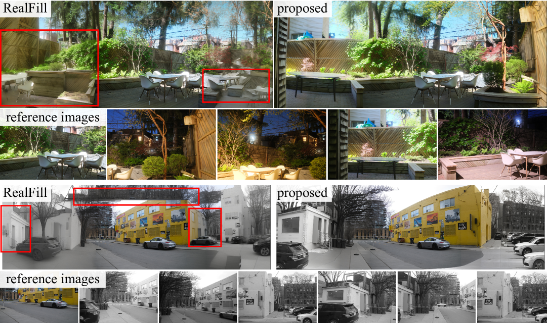
Figure 1: We introduce a generative method for panoramic image stitching from multiple casually captured reference images that exhibit strong parallax, lighting variation, and style differences. Our approach fine-tunes an inpainting diffusion model to match the content and layout of the reference images. After fine-tuning, we outpaint one reference image (e.g., the leftmost reference view shown here) to create a seamless panorama that incorporates information from the other views. Unlike prior methods such as RealFill [tang2024realfill], which produces artifacts when outpainting large scene regions (red boxes), our method more accurately preserves scene structure and spatial composition.

1 Introduction

Creating a coherent visual representation from multiple input images is a long-standing problem in computer vision [szeliski2007image, szeliski1997creating], and many techniques have been proposed to combine multiple images from different perspectives to synthesize panoramas [brown2007automatic], multi-perspective images [agarwala2006photographing, peleg2000mosaicing, seitz2003multiperspective], or photo montages [agarwala2004interactive, nomura2007scene]. More recently, image generation models make it possible to render or outpaint new image content based on one or more input images [ruiz2023dreambooth, tang2024realfill]. Inspired by methods for panorama synthesis and recent image generation techniques, we propose to address the task of generative panoramic image stitching—i.e., we seek to generate seamless panoramas that are faithful to the content of multiple reference images captured from different viewpoints with strong variations in lighting or style (Figure 1).

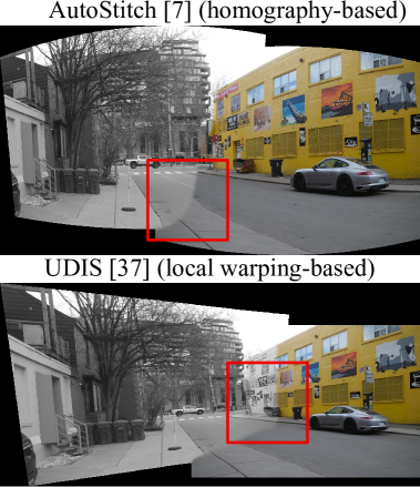
Figure 2: Conventional panoramic image stitching methods [brown2007automatic, nie2023parallax] fail to account for strong parallax effects or variations in lighting or style.

A standard approach for panoramic image stitching involves detecting feature correspondences and estimating geometric transformations between input images [brown2007automatic]. Then, the input images are warped based on the estimated transformation and blended together into a panorama [burt1983multiresolution, perez2003poisson]. Conventionally, these techniques use a homography to relate input images, which assumes that there is no parallax (i.e., no translation between captured viewpoints) [szeliski2007image]. Violating this assumption results in artifacts, such as ghosting [eden2006seamless], as shown in Figure 2 (top). Hence, a significant amount of effort has been devoted to improving robustness to viewpoint changes, e.g., by optimizing local warping operations [chang2014shape, gao2011constructing, lee2020warping, li2017parallax, liao2019single, lin2015adaptive, lin2011smoothly, zaragoza2013projective, zhang2014parallax], by using graph cuts to minimize seams between blended images [eden2006seamless, gao2013seam, zhang2014parallax], or optimizing neural networks [nie2021unsupervised, nie2023parallax], but completely avoiding artifacts is challenging when images are captured from significantly different positions. Further, standard techniques for image stitching assume that camera acquisition settings and illumination conditions are roughly constant across input images; while image blending can help to mitigate small variations in camera gain, exposure, white balance, or scene illumination [brown2007automatic, burt1983multiresolution, perez2003poisson] it fails to handle strong variations in the lighting or style of input images (Figure 2, bottom).

A separate line of work seeks to create panoramic images via image synthesis. For example, using generative models, recent approaches synthesize panoramas from a text prompt [bar2023multidiffusion, frolov2025spotdiffusion, lee2023syncdiffusion, ye2024diffpano] or inpaint masked regions of an input panorama [wu2024panodiffusion]; however, these methods do not handle the stitching of reference images with overlapping fields of view and significant parallax effects. The recent work of Tang et al. [tang2024realfill] uses a pre-trained image generation model for reference-guided inpainting, which is close to our task. Specifically, they fine-tune an image diffusion model to inpaint a set of casually captured reference images from different viewpoints and lighting conditions. After fine-tuning, the model can be used to outpaint an existing image in a way that is consistent with the content of the reference images and robust to parallax or lighting variations. However, we find that attempting to use this approach for panoramic image stitching fails, as outpainting large missing regions results in artifacts and scene layouts that are not faithful to the input reference images (see Figure 1).

Here, we address limitations of conventional methods for panoramic image stitching as well as more recent, reference-driven outpainting techniques [tang2024realfill]. Given a set of casually captured reference images, we first compute a coarse alignment of the images via conventional feature matching and homography estimation [brown2007automatic], resulting in a set of warped images and their approximate locations on an initial panorama. To correct artifacts in this initial panorama—such as those caused by parallax or lighting inconsistencies—we fine-tune [ruiz2023dreambooth] a large, pre-trained inpainting diffusion model [stablediffusioninpaint] to solve a position-aware inpainting task. Specifically, we fine-tune the model to inpaint and outpaint each warped input image while conditioning on positional encodings that reflect the image’s location within the panorama. Once fine-tuned, the model is used to iteratively outpaint the panorama from a single reference image, resulting in a seamless composite that integrates content from all reference views as shown in Figure 1.

In summary, we make the following contributions.

• We propose the task of generative panoramic image stitching, which seeks to generate panoramas that are faithful to a set of reference images containing significant parallax effects and variations in illumination or style.

• We address this task with a method that estimates the coarse layout of the reference images within a panorama and then fine-tunes a diffusion model to generate a seamless output panorama via position-aware outpainting.

• We evaluate our approach on a dataset of captured images and show state-of-the-art results for this task compared to baselines based on reference-driven image outpainting and image stitching.

2 Related Work

Our work also connects to other methods for learning-based image stitching, multi-perspective rendering, 3D reconstruction, and reference-driven outpainting.

Learning-based image stitching.

While conventional image stitching pipelines typically use feature-based homography estimation [szeliski2007image], other approaches directly regress a homography using a neural network [detone2016deep, le2020deep, nguyen2018unsupervised] or learned features [zhang2020content], which can improve performance for dynamic scenes or images with limited texture. Nie et al. [nie2021unsupervised, nie2023parallax] introduce a two-stage procedure for image stitching that first predicts a homography between two input images using a neural network and then warps the resulting image using a transformer or thin-plate splines to reduce stitching artifacts. Our procedure uses a similar two-stage approach, but we leverage a standard feature-based approach for the initial alignment [brown2007automatic], which we find generalizes well to our captured in-the-wild images. Then, instead of directly warping the input images, we leverage generative priors and position-aware inpainting and outpainting to synthesize a seamless panorama. As such, our approach scales to handle multiple input images, and we avoid stitching artifacts due to parallax or lighting variations because the output panorama is synthesized by the generative model rather than produced by warping the input images.

Multi-perspective rendering and 3D reconstruction.

It is also possible to synthesize panoramas using image-based rendering [agarwala2006photographing, anderson2016jump, liu2009content, nomura2007scene, rav2008minimal]. Given a sufficiently densely captured set of input images, one can directly capture or estimate the desired set of light rays used to assemble an output panorama or multi-perspective image [anderson2016jump, bergen1991plenoptic, levoy1996light, richardt2013megastereo]. Alternatively, one can reconstruct a 3D representation of the scene and render novel views from any desired viewpoint [rav2008minimal, wood2000surface, debevec1996modeling, buehler2001unstructured, mildenhall2021nerf]. Still, these techniques cannot be easily applied to our proposed task, where only a few images are provided as input, camera poses are unknown, and the images have inconsistencies, e.g., due to variations in camera capture settings, color palette, or lighting.

Reference-driven image editing.

Rather than directly stitching the input images, our approach generates a panorama by outpainting one of the input views using content from the others. This design is motivated by prior work on reference-driven inpainting. For instance, Yang et al.[yang2023paint] inpaint masked regions of an image using objects from a reference image depicting a different scene. Zhou et al.[zhou2021transfill] extend this idea to multiple images from the same scene. Most similar to our method, Tang et al.[tang2024realfill] fine-tune a diffusion model for reference-guided outpainting; however, their method does not incorporate scene layout information and fails in the context of panorama synthesis (see Fig.1).

3 Generative Panoramic Image Stitching

We introduce our approach by first providing a brief background on latent diffusion models. Then, we describe our method for generative panoramic image stitching based on (1) initial panorama layout estimation via homography estimation and warping, (2) fine-tuning a diffusion model for position-aware panorama inpainting and outpainting, and (3) generating a seamless panorama via iterative outpainting. An overview of the approach is shown in Figure 3.

3.1 Preliminaries: Latent Diffusion Models

Latent diffusion models [sohl2015deep] are based on a forward and reverse process that either gradually introduces noise or removes it from a latent image $\mathbf{z}_{0}$ — i.e., an image encoded into the latent space of an image autoencoder. Latent images are typically lower in resolution than conventional images and so operating in the latent space yields improvements in computation and memory [rombach2022high].

More specifically, latent diffusion models use a Markovian forward process to iteratively transform the latent image $\mathbf{z}_{0}$ into standard Gaussian noise $\mathbf{z}_{T}\sim\mathcal{N}(\mathbf{0},\mathbf{I})$ over $T$ time steps. The intermediate noisy images $\mathbf{z}_{t}$ produced during this process are defined as [ho2020denoising]

$$\mathbf{z}_{t}=\sqrt{\alpha_{t}}\mathbf{z}_{0}+\sqrt{1-\alpha_{t}}\boldsymbol{\epsilon},$$ (1)

where $\boldsymbol{\epsilon}\sim\mathcal{N}(\mathbf{0},\mathbf{I})$ and the set of values $\{\alpha_{t}\}_{t=1}^{T}$ defines a fixed noise schedule such that increasing $t$ corresponds to adding more noise. In turn, the reverse process estimates $\mathbf{z}_{t-1}$ by gradually denoising from $\mathbf{z}_{T}\sim\mathcal{N}(0,\mathbf{I})$. The clean latent image $\mathbf{z}_{0}$ is generated through a reverse diffusion process by iteratively predicting the noise $\boldsymbol{\epsilon}$ at each time step using a neural network $\Psi$. Then, applying a decoder network converts the latent image into a conventional image $\mathbf{x}$.

In the conditional reverse process, the network is trained to predict the noise by minimizing the loss

$$\mathcal{L}=\mathbb{E}_{\mathbf{z},t,\boldsymbol{\epsilon}}\parallel\Psi(\mathbf{z}_{t},t,\mathcal{C})-\boldsymbol{\epsilon}\parallel_{2}^{2}.$$ (2)

Here, the network is given a conditioning signal $\mathcal{C}$—e.g., a text prompt or a masked image for inpainting. At inference time, $\Psi$ is sampled to remove noise from $\mathbf{z}_{T}$ and iteratively estimate $\mathbf{z}_{t-1}$ until the clean latent image $\mathbf{z}_{0}$ is recovered.

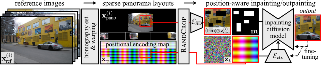
Figure 3: Method overview. Given a set of reference images $\{\mathbf{x}_{\text{ref}}^{(i)}\}_{i=1}^{N}$, we generate sparse panorama layouts $\{\mathbf{x}_{\text{pano}}^{(i)}\}_{i=1}^{N}$ by detecting features [lowe2004distinctive], estimating homographies, and warping each reference image to its location in a sparse panorama containing only that image. We then fine-tune a pre-trained inpainting diffusion model for a position-aware inpainting/outpainting task. During training, random crops are taken from the sparse panoramas and a positional encoding map $\mathbf{x}_{\gamma}$. Each panorama crop is processed using an encoder $\mathcal{E}_{\text{SD}}$, and we we multiply the resulting latent image $\mathbf{z}^{(i)}_{\text{crop}}$ with a random binary mask $(1-\mathbf{m})$. We process the crop of $\mathbf{x}_{\gamma}$ with an encoder $\mathcal{E}_{\text{ctx}}$ and use the result to condition the diffusion model. The other inputs — the masked version of $\mathbf{z}_{\text{crop}}^{(i)}$, the mask $\mathbf{m}$, and the noisy latent image $\mathbf{z}_{t}$ — are concatenated together and passed as input to the model. After fine-tuning, we generate seamless panoramas by outpainting one of the initial sparse panoramas.

3.2 Panorama Layout Estimation & Positional Encoding

Given a set of $N$ input reference images $\{\mathbf{x}_{\text{ref}}^{(i)}\}_{i=1}^{N}$, where $\mathbf{x}_{\text{ref}}^{(i)}\in\mathbb{R}_{+}^{H_{\text{ref}}\times W_{\text{ref}}\times 3}$, we aim to generate a panorama $\mathbf{x}_{\text{pano}}\in\mathbb{R}^{H_{\text{pano}}\times W_{\text{pano}}\times 3}$ via latent diffusion that seamlessly stitches together scene content from the reference views and outpaints uncaptured scene regions.

The first step in this procedure involves producing an initial panorama layout via homography estimation and warping. We adapt the procedure of Brown et al. [brown2007automatic] to detect feature correspondences between the input images, estimate homographies, and warp each image into cylindrical coordinates. The result of this procedure is a set of sparse panoramas $\{\mathbf{x}_{\text{pano}}^{(i)}\}_{i=1}^{N}$, $\mathbf{x}_{\text{pano}}^{(i)}\in\mathbb{R}_{+}^{H_{\text{pano}}\times W_{\text{pano}}\times 3}$, which each contains a single warped reference image (see Figure 3).

We also associate the panorama with a positional encoding map $\mathbf{x}_{\gamma}$ [mildenhall2021nerf]. The map is computed using a function $\gamma(p)=[\cos(\pi f_{1}p),\sin(\pi f_{1}p),\ldots,\cos(\pi f_{F}p),\sin(\pi f_{F}p)]^{T}$, where $\{f_{i}\}_{i=1}^{F}$ are the encoding frequencies, and the function $\gamma(\cdot)$ is applied to each vertical and horizontal pixel coordinate $p$. Encoding each pixel coordinate results in $\mathbf{x}_{\gamma}\in\mathbb{R}^{H_{\text{pano}}\times W_{\text{pano}}\times 4F}$, where $F$ is the number of positional encoding frequencies. Additional details are provided in Supp. Section S1.1.

3.3 Fine-tuning for Position-aware Inpainting and Outpainting

We use the set of panoramas $\{\mathbf{x}_{\text{pano}}^{(i)}\}_{i=1}^{N}$ and the positional encoding map $\mathbf{x}_{\gamma}$ to fine-tune an inpainting diffusion model for position-aware inpainting and outpainting.

Architecture.

Our approach adapts a pre-trained inpainting diffusion model $\Psi(\mathbf{z}_{t},t,\mathcal{C})$ (we use Stable Diffusion 2.1 [stablediffusioninpaint]). The model is conditioned on the input

$$\mathcal{C}=\{\mathbf{m},(1-\mathbf{m})\odot\mathbf{z}_{\text{crop}}^{(i)},\mathbf{c}_{\text{ctx}}\},$$ (3)

where $\mathbf{m}$ is a randomly generated binary mask to be inpainted or outpainted, $\odot$ indicates Hadamard product, and $\mathbf{z}_{\text{crop}}^{(i)}$ is a randomly cropped region of $\mathbf{x}_{\text{pano}}^{(i)}$ that we encode into the latent space using the Stable Diffusion encoder $\mathcal{E}_{\text{SD}}$, or $\mathbf{z}_{\text{crop}}^{(i)}=\mathcal{E}_{\text{SD}}(\textsc{RandCrop}(\mathbf{x}_{\text{pano}}^{(i)}))$. The context embedding tensor $\mathbf{c}_{\text{ctx}}$ is produced as $\mathbf{c}_{\text{ctx}}=\mathcal{E}_{\text{ctx}}(\textsc{RandCrop}(\mathbf{x}_{\gamma}))$, where we apply the same random crop to the positional encoding map $\mathbf{x}_{\gamma}$ as for $\mathbf{x}_{\text{pano}}^{(i)}$. We process the cropped version of $\mathbf{x}_{\gamma}$ using $\mathcal{E}_{\text{ctx}}$, a small three-layer convolutional encoder with a linear layer (see Supp. Section S1.2).

While the context embedding tensor $\mathbf{c}_{\text{ctx}}$ is used by the pre-trained model for text conditioning, our approach repurposes it to encode the positional information, and we provide the tensor as input to the cross-attention layers of the network. The other conditioning signals (i.e., $\mathbf{m}$ and $(1-\mathbf{m})\odot\mathbf{z}_{\text{crop}}^{(i)}$) are concatenated with the noisy latent image $\mathbf{z}_{t}$ and passed as input to the diffusion model. A more detailed description of the architecture is provided in Supp. Section S1.

Optimization.

We fine-tune the network $\Psi$ to minimize the loss function

$$\mathcal{L}=\mathbb{E}_{\boldsymbol{\epsilon},\mathbf{z}_{\text{crop}}^{(i)},i,t,\mathbf{m}}\left[\left\|\mathbf{m}_{\text{valid}}\odot\left(\Psi(\mathbf{z}_{\text{crop},t}^{(i)},t,\mathcal{C})-\boldsymbol{\epsilon}\right)\right\|_{2}^{2}\right],$$ (4)

where $\mathbf{m}_{\text{valid}}$ is a binary mask that restricts the loss to regions of $\mathbf{z}_{\text{crop}}^{(i)}$ that correspond to non-empty areas in the cropped sparse panorama $\mathbf{x}_{\text{pano}}^{(i)}$. Hence, we fine-tune the model to minimize the difference between the noise it predicts and the noise added to $\mathbf{z}^{(i)}_{\text{crop}}$, where $\mathbf{z}^{(i)}_{\text{crop},t}=\sqrt{\alpha_{t}}\mathbf{z}^{(i)}_{\text{crop}}+\sqrt{1-\alpha_{t}}\boldsymbol{\epsilon}$ (as described in Equation 1).

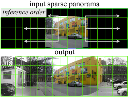
Figure 4: Panorama generation. We use the fine-tuned model to iteratively outpaint each tile (green grid) of the panorama, in order of distance from the center (white arrows), to create a seamless result.

We use low-rank adaptation (LoRA) [hu2022lora] to optimize the model’s self-attention layers and preserve the capabilities of the Stable Diffusion model’s pre-trained weights. The cross-attention layers undergo full-parameter fine-tuning to better adapt to the positional encoding information provided by $\mathbf{c}_{\text{ctx}}$. Last, we initialize and optimize all parameters of the context encoder $\mathcal{E}_{\text{ctx}}$.

3.4 Panorama Generation

After fine-tuning, we generate a seamless panorama $\mathbf{x}_{\text{pano}}$ by outpainting one of the initial sparse panoramas $\mathbf{x}_{\text{pano}}^{(i)}$. The main challenge in this step is that the resolution of the panorama is much larger than the nominal resolution for which the inpainting diffusion model is trained—so we cannot generate the entire panorama in a single inference pass. Instead, we sequentially denoise tiles of the panorama to generate the final output as depicted in Figure 4. We apply the sequential denoising procedure to the sparse panorama containing a centered warped reference image — this is an arbitrary image to which we register the other reference images during the initial layout estimation process (Section 3.2).

Specifically, we generate an evenly spaced grid of overlapping image tiles or boxes $\{\mathbf{b}^{(i)}\}_{i=1}^{B}$ across the panorama, where $\mathbf{b}^{(i)}=\{x^{(i)},y^{(i)},H,W\}$ gives the pixel coordinates of the corner of the tile and the height and width of the tile. In practice, we use $20\%$ overlap between tiles, and we set $H=W=512$. After positioning the tiles, if some tiles extend beyond the extent of the panorama, the overlap is reduced until all tiles fit within the panorama in both the vertical and horizontal dimensions. For each tile in the grid, we run the full reverse diffusion process using the DDPM sampler [ho2020denoising] to inpaint/outpaint the missing regions of the tile. Inpainting/outpainting masks are feathered and composited with the current state of the generated panorama $\mathbf{x}_{\text{pano}}$. Different than training, where we randomly sample the mask values $\mathbf{m}$, during inference we set the $\mathbf{m}$ values to indicate which regions of each input tile have not yet been generated. The tiles are denoised in order of increasing distance from their centroids to that of the warped reference image. We summarize this procedure in Algorithm 1.

Input: $\mathbf{x}_{\text{pano}}^{(0)}$ $\blacktriangleleft$ Input sparse panorama

     $\mathbf{x}_{\gamma}$   $\blacktriangleleft$ Positional encoding map

     $\{\mathbf{b}^{(i)}\}_{i=1}^{B}$ $\blacktriangleleft$ Tiles covering panorama

Output: Panorama $\mathbf{x}_{\text{pano}}$ with all tiles denoised

// Order tiles based on distance

$[\mathbf{b}^{(1)},\mathbf{b}^{(2)},\ldots,\mathbf{b}^{(B)}]\leftarrow\textsc{OrderByDist}(\{\mathbf{b}^{(i)}\}_{i=1}^{B})$

for $i=1$ to $B$ do

    // Initialize noisy latent by adding noise to reference latent

    $\mathbf{z}_{\mathbf{b}^{(i)},T}\leftarrow\mathcal{E}_{\text{SD}}(\mathbf{x}^{(0)}_{\text{pano}}[\mathbf{b}^{(i)}])+\boldsymbol{\epsilon},\quad\boldsymbol{\epsilon}\sim\mathcal{N}(0,\sigma^{2}I)$

    $\mathbf{c}_{\text{ctx}}\leftarrow\mathcal{E}_{\text{ctx}}(\mathbf{x}_{\gamma}[\mathbf{b}^{(i)}])$

    $\mathbf{m}\leftarrow\textsc{GetRegionToInpaint}(\mathbf{z}_{\mathbf{b}^{(i)},T})$

    for $t=T$ to $1$ do

       // Denoise tile

       $\mathbf{z}_{\mathbf{b}^{(i)},t-1}\leftarrow\textsc{Denoise}(\mathbf{z}_{\mathbf{b}^{(i)},t},\mathbf{m},(1-\mathbf{m})\odot\mathbf{z}_{\mathbf{b}^{(i)},t-1},\mathbf{c}_{\text{ctx}})$

   // Update output with denoised tile using latent decoder $\mathcal{D}_{\text{SD}}$

    $\mathbf{x}_{\text{pano}}[\mathbf{b}^{(i)}]\leftarrow\textsc{Composite}(\mathbf{x}_{\text{pano}}[\mathbf{b}^{(i)}],\mathcal{D}_{\text{SD}}(\mathbf{z}_{\mathbf{b}^{(i)},0}))$

return $\mathbf{x}_{\text{pano}}$

Algorithm 1 Panorama Generation

3.5 Implementation Details

Masking and augmentation.

Inpainting masks are synthesized with randomly generated patterns following Tang et al. [tang2024realfill]. We also introduce an augmentation scheme which perturbs the location of the warped images in the sparse panorams with a random similarity transformation. We find that this helps to avoid seams from appearing in the final output panoramas at the boundary locations of the warped images.

Training and inference.

We apply LoRA to the Stable Diffusion model’s self-attention layers and fully fine-tune the cross-attention layers and $\mathcal{E}_{\text{ctx}}$, using AdamW with learning rates of $1\text{\times}{10}^{-4}$ (LoRA), $3\text{\times}{10}^{-4}$ (cross-attention), and $8\text{\times}{10}^{-4}$ ($\mathcal{E}_{\text{ctx}}$). Training runs for 4,000 iterations with batch size 32 and takes 4.5 hours on 2$\times$A100 GPUs. At inference, a $1000\times 3000$ panorama typically takes 1 minute to generate on a single RTX 2080 Ti. We use classifier-free guidance [ho2021classifier] with $\mathbf{c}_{\text{ctx}}=0$ and a guidance scale of 1.5.

Correspondence-based seed selection.

We employ a correspondence-based seed selection process [tang2024realfill] to identify generated panoramas whose layout matches the result of feature-based image registration [brown2007automatic]. Specifically, we generate ten panoramas with different random seeds and take our output to be the panorama with the most feature matches (computed with LoFTR [sun2021loftr]) compared to the reference. Please see Supp. Section S1 for additional implementation details.

4 Experiments

Dataset.

We collect two image datasets of eight scenes each, with several images captured for each scene. One dataset consists of tripod-captured images collected by rotating a camera on a tripod, and a set of casually captured images from different scene viewpoints using a handheld camera (Fujifilm X100 VI). In the casually captured dataset, the distance between viewpoints varies by up to one to two meters, and we also introduce other challenging variations, such as capturing images of the same scene with varying illumination conditions, camera white balance, or image color palette.

The tripod-captured dataset, with minimal parallax, aligns with assumptions of standard stitching methods and is used to compute a reference panorama for evaluating image quality. The casually captured dataset tests robustness to parallax, illumination, and style variations. A detailed description of the captured scenes and the number of captured images for each scene is provided in Supp. Section S1.6.

To facilitate comparison across output panoramas, we include one tripod-captured image within the set of casually captured images. We configure our method and all baselines so that this shared image is placed at the center of the output panorama, ensuring a consistent layout across output panoramas from both sets of images.

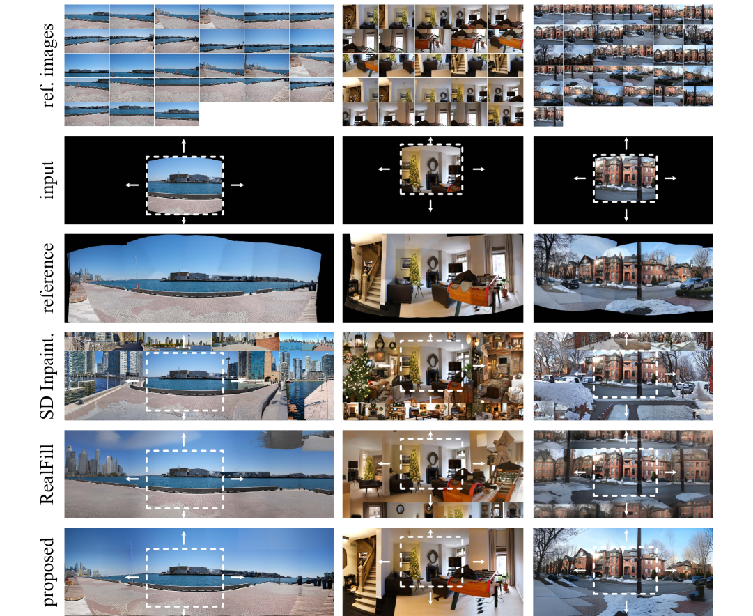
Figure 5: Qualitative results on the tripod-captured dataset. We find that our approach produces panoramas that are more consistent with the layout and content of the reference panorama than baseline approaches based on inpainting/outpainting.

Method	PSNR (dB) $\uparrow$	SSIM $\uparrow$	LPIPS $\downarrow$	DreamSim $\downarrow$	DINO $\uparrow$	CLIP $\uparrow$	LoFTR (L2 Distance) $\downarrow$	LoFTR (Matching) $\uparrow$
SD2	9.97 (0.74)	0.267 (0.099)	0.650 (0.040)	0.295 (0.050)	0.916 (0.031)	0.859 (0.074)	85.45 (56.00)	0.012 (0.003)
RealFill	11.71 (1.61)	0.366 (0.143)	0.559 (0.069)	0.198 (0.040)	0.952 (0.020)	0.918 (0.048)	43.01 (35.07)	0.030 (0.010)
proposed	12.11 (2.05)	0.388 (0.136)	0.453 (0.077)	0.107 (0.031)	0.974 (0.019)	0.941 (0.033)	15.11 (7.60)

Table 1: Quantitative assessment of generative panoramic image stitching on the tripod-captured image dataset. We outpaint a single warped reference image (see Figure 5), and compare the generated result to a reference panorama produced using AutoStitch [brown2007automatic]. Our approach generates panoramas that are most faithful to the reference images. Standard deviations are reported in parentheses.

Baselines.

We compare our approach to multiple baselines, starting with the conventional image stitching method of Brown and Lowe [brown2007automatic] (AutoStitch), which uses feature matching, homography estimation, warping, and blending. We chose this baseline because (1) it informs our own panorama layout estimation step, and (2) we found, through empirical evaluation, that it was more robust than other methods for parallax-tolerant stitching. In particular, we found AutoStitch’s bundle adjustment procedure more effective for stitching multiple images than recent methods tailored to pairwise stitching or reliant on pre-trained networks, which failed to generalize to our captured image datasets.

We also compare to the Stable Diffusion 2 inpainting model [stablediffusioninpaint], which serves as the backbone of our method. This baseline omits our positional encoding and fine-tuning strategy, but follows the same iterative outpainting procedure. Additionally, we compare to RealFill [tang2024realfill], using their inpainting-based fine-tuning strategy and generating panoramas using our iterative outpainting process. For the Stable Diffusion 2 baseline, we use a guidance scale of $7.5$ during inference, and for RealFill we follow their implementation and do not use guidance.

Metrics.

We evaluate our method using standard image quality metrics, learning-based metrics that assess high-level image structure, and feature-matching-based metrics that assess how well our approach preserves the scene layout. Specifically, we use standard image quality metrics: peak signal-to-noise ratio, structure similarity [wang2004image], and learned perceptual image patch similarity [zhang2018unreasonable]. To evaluate high-level image structure, we use DreamSim [fu2023dreamsim], which assesses similarity in semantic content and layout. We also compute the cosine similarity between the DINO [caron2021emerging] and CLIP [radford2021learning] full-image embeddings. Additionally, we use image feature matches from LoFTR [sun2021loftr] to assess how well the layout of the output panorama matches a reference. We report both the L2 distance between the pixel coordinates of matching features and the number of matched features divided by the total number of features in the reference image (see Supp. Section S1.8 for more details).

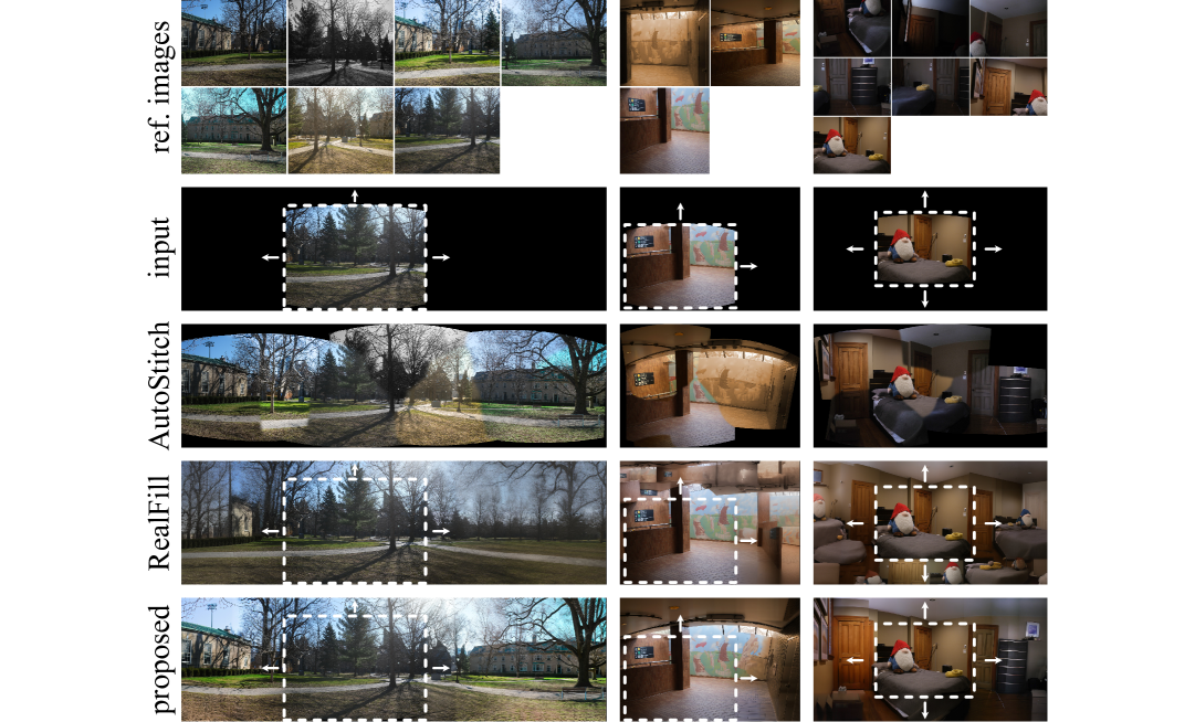
Figure 6: Qualitative results on the casually captured dataset. Even in this challenging scenario, where the input images have strong parallax effects and variations in style, illumination, color palette, or camera capture settings, our approach reconstructs seamless panoramas that preserve the content and layout of the reference.

Supplementary Material

S1 Supplementary Implementation Details

S1.1 Data Preparation

We use reference images capturing a scene from multiple viewpoints to build a panorama. Images are aligned via homography-based registration and warped onto a panorama of size $H_{\text{pano}}\times W_{\text{pano}}$ using homography matrices $\mathbf{H}_{i}$, computed with feature matching (we use SIFT [lowe2004distinctive, brown2007automatic]).

A global positional encoding $\mathbf{x}_{\gamma}\in\mathbb{R}^{H_{\text{pano}}\times W_{\text{pano}}\times C}$, with $C\in\{4,8,12\}$, encodes spatial patterns. Coordinates $x\in[0,W_{\text{pano}}]$, $y\in[0,H_{\text{pano}}]$ are normalized:

$$p_{x}=\frac{2x-W_{\text{pano}}}{W_{\text{pano}}},\quad p_{y}=\frac{2y-H_{\text{pano}}}{H_{\text{pano}}}.$$

Frequencies are:

$$f_{i}=\exp\left(\log f_{\text{min}}+\frac{i(\log f_{\text{max}}-\log f_{\text{min}})}{F}\right),\quad i=0,\ldots,F-1.$$

The encoding is:

$$\mathbf{x}_{\gamma}(y,x,c)=\begin{cases}\sin(\pi p_{x}f_{c/2}),&c=2i,\\ \cos(\pi p_{x}f_{c/2}),&c=2i+1,\\ \sin(\pi p_{y}f_{(c-2F)/2}),&c=2F+2i,\\ \cos(\pi p_{y}f_{(c-2F)/2}),&c=2F+2i+1,\end{cases}$$

where $F=C/4$ is the number of frequencies per dimension, $i=0,\ldots,F-1$, and $c$ denotes the channel index. In our proposed method, we use $f_{\text{min}}=1$, $f_{\text{max}}=50$ and $C=12$.

S1.2 Positional Encoding Processing

A crop of the global positional encoding $\mathbf{x}_{\gamma}[\mathbf{b}]\in\mathbb{R}^{H_{\text{pano}}\times W_{\text{pano}}\times C}$, where $\mathbf{b}=\{x,y,W=512,H=512\}$, is transformed into context embeddings $\mathbf{c}_{\text{ctx}}\in\mathbb{R}^{B\times 77\times 1024}$ (where $B$ is the batch size) through a convolutional processing module. The transformation proceeds as follows:

$$F_{1} =\text{GELU}\left(\text{Conv2D}(\mathbf{x}_{\gamma}[\mathbf{b}],\ \text{kernel}=4,\ \text{stride}=2,\ \text{padding}=1,\ \text{out}=128)\right),$$

$$F_{2} =\text{GELU}\left(\text{Conv2D}(F_{1},\ \text{kernel}=4,\ \text{stride}=2,\ \text{padding}=1,\ \text{out}=128)\right),$$

$$F_{3} =\text{AdaptiveAvgPool2D}(F_{2},\ (7,\ 11)),$$

reducing the spatial dimensions from $512\times 512$ to $7\times 11$. The feature map is then reshaped and projected to a higher-dimensional space:

$$F_{4} =\text{Reshape}(F_{3},\ (B,\ 77,\ 128)),$$

$$F_{5} =\text{Linear}(F_{4},\ \text{out}=1024),$$

yielding $F_{5}\in\mathbb{R}^{B\times 77\times 1024}$. A token-level positional encoding inspired by transformer-based language models [vaswani2017attention] is added to $F_{5}$. This encoding is precomputed for all 77 token positions and uses sinusoidal functions to encode each token’s position in the sequence. For each token index $p\in\{0,1,\ldots,76\}$, its corresponding embedding $PE(p)\in\mathbb{R}^{1024}$ is defined by:

$$PE(p,2i)=\sin\left(p/10000^{2i/d}\right),\quad PE(p,2i+1)=\cos\left(p/10000^{2i/d}\right),$$

for $i\in\{0,1,\ldots,d/2-1\}$, where $d=1024$ is the embedding dimension. The token positional encoding is added to $F_{5}$, i.e., $F_{6}=F_{5}+PE$, where $PE\in\mathbb{R}^{77\times 1024}$ is broadcast across the batch dimension. Finally, a layer normalization is applied:

$$\mathbf{c}_{\text{ctx}}=\text{LayerNorm}(F_{6}),$$

producing the final context embeddings $\mathbf{c}_{\text{ctx}}\in\mathbb{R}^{B\times 77\times 1024}$, which are used as input to the pre-trained inpainting diffusion model’s cross-attention layers. The entire positional encoding processor network is trained from scratch, allowing it to optimally learn the transformation from spatial positional encodings to meaningful context embeddings for the panorama inpainting and outpainting task.

S1.3 Attention Mechanisms

The model employs self-attention and cross-attention to integrate internal features across multiple views and enforce spatial consistency, respectively.

S1.3.1 Self-Attention

Self-attention operates on the latent feature map $\mathbf{z}\in\mathbb{R}^{B\times C\times H\times W}$ (e.g., $C=320,H=W=64$), flattened to $\mathbf{z}_{\text{flat}}\in\mathbb{R}^{B\times N\times C}$ where $N=H\times W$. We use multi-head attention, with $h$ heads, each processing a subspace of dimension $d_{\text{head}}=C/h$:

$$Q_{i}=\mathbf{z}_{\text{flat}}W_{q,i},\quad K_{i}=\mathbf{z}_{\text{flat}}W_{k,i},\quad V_{i}=\mathbf{z}_{\text{flat}}W_{v,i},$$

where $W_{q,i},W_{k,i},W_{v,i}\in\mathbb{R}^{C\times d_{\text{head}}}$. Attention scores are computed as:

$$A_{\text{head},i}=\frac{Q_{i}K_{i}^{\top}}{\sqrt{d_{\text{head}}}}\in\mathbb{R}^{B\times N\times N},$$

with outputs aggregated across heads:

$$\text{Attention}_{\text{self}}=\text{Concat}(\text{Attention}_{\text{head},1},\dots,\text{Attention}_{\text{head},h})W_{o},$$

where $W_{o}\in\mathbb{R}^{C\times C}$. This enables global spatial reasoning, crucial for maintaining coherence across different views in the final panoramic image.

S1.3.2 Cross-Attention

Cross-attention integrates context embeddings $\mathbf{c}_{\text{ctx}}\in\mathbb{R}^{B\times 77\times 1024}$ with $\mathbf{z}_{\text{flat}}$

$$Q_{i}=\mathbf{z}_{\text{flat}}W_{q,i}^{\text{cross}},\quad K_{i}=\mathbf{c}_{\text{ctx}}W_{k,i}^{\text{cross}},\quad V_{i}=\mathbf{c}_{\text{ctx}}W_{v,i}^{\text{cross}},$$

where $W_{q,i}^{\text{cross}}\in\mathbb{R}^{C\times d_{\text{head}}}$, and $W_{k,i}^{\text{cross}},W_{v,i}^{\text{cross}}\in\mathbb{R}^{1024\times d_{\text{head}}}$. The output is

$$\text{Attention}_{\text{cross}}=\text{Concat}(\text{Attention}_{\text{cross},1},\dots,\text{Attention}_{\text{cross},h})W_{o}^{\text{cross}},$$

ensuring inpainted regions align with the spatial context, preserving consistent features like textures and lighting across multiple input views.

S1.4 Inpainting Model Architecture and Inputs

The architecture backbone is based on the Stable Diffusion 2.1 inpainting model [stablediffusioninpaint], which uses an encoder–decoder UNet architecture with embedded self-attention and cross-attention layers for multi-scale reasoning. The denoising process follows the DDPM framework [ho2020denoising], where a noisy latent representation is progressively refined to reconstruct the image.

As described in the main paper, we adapt the pre-trained inpainting diffusion model $\Psi(\mathbf{z}_{\text{crop},t}^{(i)},t,\mathcal{C})$ where

$$\mathcal{C}=\{\mathbf{m},(1-\mathbf{m})\odot\mathbf{z}_{\text{crop}}^{(i)},\mathbf{c}_{\text{ctx}}\},$$ (S1)

Noisy Latent Input.

During training, the input noisy latent input $\mathbf{z}^{(i)}_{\text{crop},t}$ is generated by corrupting the encoded latent of a random crop from the input panorama set $\{\mathbf{x}_{\text{pano}}^{(i)}\}_{i=1}^{N}$ with noise, as

$$\mathbf{z}_{\text{crop}}^{(i)}=\mathcal{E}_{\text{SD}}(\textsc{RandCrop}(\mathbf{x}_{\text{pano}}^{(i)})),$$

where the noisy latent is then

$$\mathbf{z}^{(i)}_{\text{crop},t}=\sqrt{\alpha_{t}}\mathbf{z}^{(i)}_{\text{crop}}+\sqrt{1-\alpha_{t}}\boldsymbol{\epsilon}$$

Conditioned Input and Mask.

Following Stable Diffusion 2.1, the inpainting mask $\mathbf{m}\in\{0,1\}^{B\times 1\times 64\times 64}$ is a downsampled representation of the region to be inpainted. It is constructed by combining random shapes with warped boundary regions to simulate occlusion patterns. The conditioning input, $\mathbf{z}_{\text{crop}}^{(i)}$, is masked by $(1-\mathbf{m})$ to simulate occlusion and then concatenated with the mask itself and the noised latent $\mathbf{z}_{t}$ as input to the UNet.

Context Embeddings.

The embeddings $\mathbf{c}_{\text{ctx}}\in\mathbb{R}^{B\times 77\times 1024}$ are derived from the same crop dimensions used for $\mathbf{z}_{\text{crop}}^{(i)}$, applied to the positional encoding map $\mathbf{x}_{\gamma}$ and passed through the context encoder $\mathcal{E}_{\text{ctx}}$:

$$\mathbf{c}_{\text{ctx}}=\mathcal{E}_{\text{ctx}}(\textsc{RandCrop}(\mathbf{x}_{\gamma})).$$

These embeddings replace text conditioning and are fed into the cross-attention blocks of the UNet (see Section S1.3.2), enabling spatially-aware denoising. This conditioning scheme enables the model to perform both inpainting and outpainting with spatial coherence.

S1.5 Training

Training begins by sampling a latent representation $\mathbf{z}_{\text{crop}}^{(i)}$ and the corresponding positional embedding $\mathbf{c}_{\text{ctx}}$ as explained in  S1.4. The diffusion model $\Psi(\mathbf{z}_{\text{crop},t}^{(i)},t,\mathcal{C})$ is trained to predict the noise added to the latent during the forward diffusion process by minimizing the loss function Equation 1.

Optimization Strategy.

The model parameters are optimized using the AdamW optimizer. To preserve the generative power of the pre-trained Stable Diffusion model, we adopt a selective fine-tuning approach:

• LoRA (Low-Rank Adaptation) [hu2022lora] is applied to the self-attention layers of the UNet to enable efficient adaptation with fewer trainable parameters. We use a learning rate of $1\text{\times}{10}^{-4}$.

• Cross-attention layers are fully fine-tuned to allow better integration of positional context via $\mathbf{c}_{\text{ctx}}$. We use a learning rate of $3\text{\times}{10}^{-4}$.

• The VAE encoder/decoder and other layers of the UNet remain frozen to retain the fidelity of the original image reconstruction.

• The context encoder $\mathcal{E}_{\text{ctx}}$, which produces $\mathbf{c}_{\text{ctx}}$, is trained from scratch using standard initialization. We use a learning rate of $8\text{\times}{10}^{-4}$.

S1.6 Dataset

Figure S1 and Figure S2 show the reference images for the tripod-captured and casually-captured datasets, respectively. Both include the same eight scenes, captured (for the most part) at the exact same time: variations in lighting or time of day are captured in the casually captured set. The tripod-captured dataset attempts to capture a complete coverage of the scene, while the casually-captured dataset includes variations that make conventional stitching methods like AutoStitch [brown2007automatic] difficult. Specifically, we outline the variations for each scene as follows:

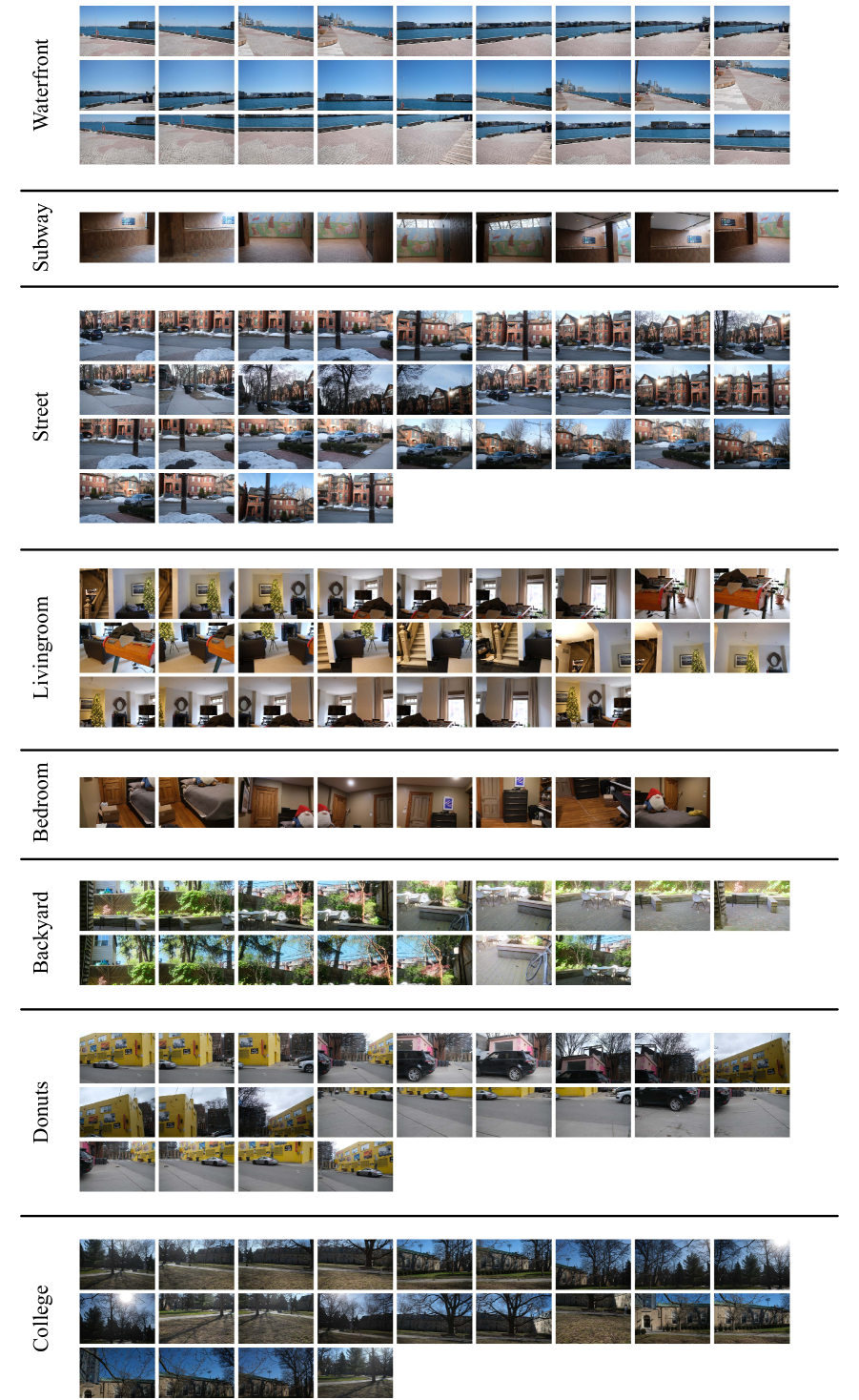
Figure S1: Reference images for the the tripod-captured dataset. Eight scenes were captured, showing a range of contexts.

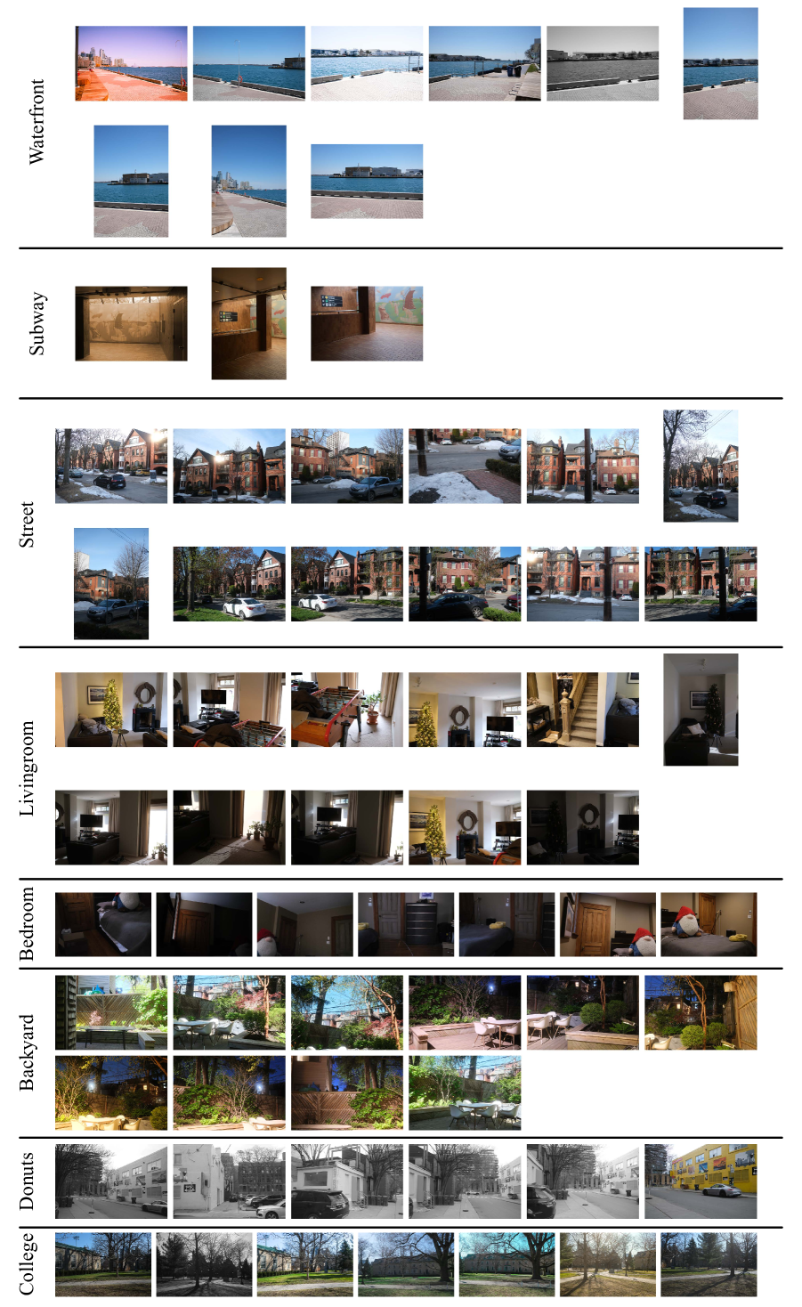
Figure S2: Reference images for the casually captured dataset. Eight scenes were captured, mirroring the tripod-captured dataset. This dataset shows challenging scenarios, where the input images have strong parallax effects (“Waterfront”, “Donuts”), variations in style (“Waterfront”, “Subway”), illumination (“Bedroom”, “Backyard”), color palette (“Waterfront”, “Donuts”, “College”), or seasonal changes (“Street”).

S1.7 Baseline Implementation Details

RealFill [tang2024realfill].

We follow the default implementation guidelines and code for RealFill. We use the default prompt “a photo of sks” and guidance scale of $0.99$ (as used in the original work) during inference. RealFill employs a simple prompt fine-tuning strategy as proposed in [ruiz2023dreambooth], where each reference image is randomly cropped during training and fine-tuned with the same input prompt. RealFill uses random masking during training and samples each reference image with equal probability.

SD2 Inpainting.

We use ChatGPT to generate the following text prompts to inpaint scenes in our dataset using the Stable Diffusion 2 inpainting [stablediffusioninpaint] baseline. We fed it the reference images and asked it to describe the scene for an in/outpainting task. We use the default guidance scale of $7.5$.

S1.8 Metrics

To evaluate the quality of generated panoramic images, we employ a comprehensive set of metrics that assess standard image quality, high-level image structure, and preservation of scene layout. The latter two use learning-based metrics and feature-matching-based metrics, respectively. We evaluate generated panoramas $\mathbf{x}_{\text{pano}}^{\text{gen}}\in\mathbb{R}_{+}^{H_{\text{pano}}\times W_{\text{pano}}\times 3}$ against the reference panorama produced using AutoStitch [brown2007automatic] on the tripod-captured dataset $\mathbf{x}_{\text{pano}}^{\text{ref}}\in\mathbb{R}_{+}^{H_{\text{pano}}\times W_{\text{pano}}\times 3}$. All metrics except DreamSim, CLIP, and DINO omit the region of the sparse panorama provided as input during inference (defined by a binary mask $\mathbf{m}_{\text{input}}\in\{0,1\}^{H_{\text{pano}}\times W_{\text{pano}}}$) to focus on inpainted areas. Below, we describe each metric, its implementation details, and its significance.

PSNR (Peak Signal-to-Noise Ratio).

Measures pixel-level similarity [hore2010image], defined as

$$\texttt{PSNR}=10\cdot\log_{10}\left(\frac{\texttt{MAX}_{\bf{x}}^{2}}{\texttt{MSE}(\mathbf{x}_{\text{pano}}^{\text{ref}},\mathbf{x}_{\text{pano}}^{\text{gen}})}\right),$$

where $\texttt{MAX}_{\bf{x}}=255$ for 8-bit RGB images, and $\texttt{MSE}(\cdot)$ is the mean squared error between valid pixels (i.e., where $\mathbf{m}_{\text{input}}=0$) of $\mathbf{x}_{\text{pano}}^{\text{ref}}$ and $\mathbf{x}_{\text{pano}}^{\text{gen}}$. Higher values indicate better pixel fidelity.

SSIM (Structural Similarity Index).

Assesses structural and perceptual similarity by comparing luminance, contrast, and structure in grayscale images [wang2004image]:

$$\texttt{SSIM}(x,y)=\frac{(2\mu_{x}\mu_{y}+c_{1})(2\sigma_{xy}+c_{2})}{(\mu_{x}^{2}+\mu_{y}^{2}+c_{1})(\sigma_{x}^{2}+\sigma_{y}^{2}+c_{2})},$$

where $\mu_{x},\mu_{y}$ are means, $\sigma_{x},\sigma_{y}$ are variances, $\sigma_{xy}$ is covariance, and $c_{1},c_{2}$ are constants. We compute SSIM on grayscale images with masked regions ($\mathbf{m}_{\text{input}}=1$) set to zero. Higher values indicate better structural consistency.

LPIPS (Learned Perceptual Image Patch Similarity).

Measures perceptual similarity using a pre-trained AlexNet [krizhevsky2012imagenet], as proposed by Zhang et al. [zhang2018unreasonable]. For permuted image tensors $\mathbf{x}_{\text{pano}}^{\text{ref}},\mathbf{x}_{\text{pano}}^{\text{gen}}\in\mathbb{R}_{+}^{B\times 3\times H_{\text{pano}}\times W_{\text{pano}}}$, normalized to $[-1,1]$, LPIPS computes feature distances as

$$\texttt{LPIPS}=\frac{1}{H^{\prime}W^{\prime}}\sum_{h,w}\texttt{loss}_{\texttt{Alex}}(\mathbf{x}_{\text{pano}}^{\text{ref}},\mathbf{x}_{\text{pano}}^{\text{gen}})\cdot(1-\mathbf{m}_{\text{input}}^{\prime}),$$

where $\texttt{loss}_{\texttt{Alex}}$ is the weighted L2 distance between feature activations from AlexNet layers, $\mathbf{m}_{\text{input}}^{\prime}$ is the resized mask, and $H^{\prime},W^{\prime}$ match the feature map size. Lower values indicate better perceptual similarity.

DreamSim [fu2023dreamsim].

Evaluates high-level perceptual similarity using the DreamSim model trained on human perceptual judgments. The metric is:

$$\texttt{DreamSim}=\texttt{dreamsim\_model}(\mathbf{x}_{\text{pano}}^{\text{ref}^{\prime}},\mathbf{x}_{\text{pano}}^{\text{gen}^{\prime}}),$$

where $\mathbf{x}_{\text{pano}}^{\text{ref}^{\prime}},\mathbf{x}_{\text{pano}}^{\text{gen}^{\prime}}$ are images resized to $224\times 224$ to match the model’s input requirements. The DreamSim model, based on a vision transformer, predicts perceptual similarity by comparing feature embeddings. Lower scores indicate closer perceptual alignment.

DINO.

Measures semantic similarity using the DINOv2-base model [oquab2023dinov2] as the cosine distance between features extracted from the last hidden state:

$$\texttt{DINO}=\frac{\cos(\texttt{feat}^{\text{ref}},\texttt{feat}^{\text{gen}})+1}{2},$$

where $\texttt{feat}^{\text{ref}},\texttt{feat}^{\text{gen}}$ are mean-pooled features from the last hidden state of DINOv2, and $\cos(\cdot)$ is the cosine similarity. Higher values indicate better semantic alignment.

CLIP.

Assesses semantic similarity using the CLIP ViT-B/32 model [radford2021learning]. The CLIP score is defined as the cosine similarity between normalized CLIP image embeddings:

$$\texttt{CLIP}=\cos(\mathbf{z}^{\text{ref}}_{\texttt{clip}},\mathbf{z}^{\text{gen}}_{\texttt{clip}}),$$

where $\mathbf{z}^{\text{ref}}_{\texttt{clip}},\mathbf{z}^{\text{gen}}_{\texttt{clip}}$ are image embeddings from the forward pass of the CLIP ViT-B/32 model. Higher values indicate better semantic consistency.

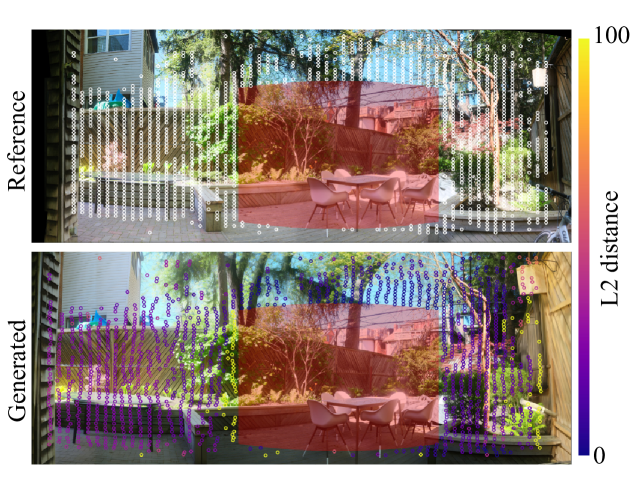
Figure S3: Example of LoFTR feature matching between reference and generated panoramas. White circles mark selected keypoints in the reference, with corresponding points in the generated panorama color-coded by L2 pixel distance from their reference positions.

LoFTR Metrics.

Evaluates feature correspondence using LoFTR [sun2021loftr]. Images are resized to $512\times 512$ and converted to grayscale and then processed. We report both the L2 distance between the pixel coordinates of matching features and the number of matched features divided by the total number of features in the reference image. Specifically,

$$\texttt{LoFTR\_L2\_Distance}=\frac{1}{N}\sum_{i=1}^{N}\sqrt{\sum(\texttt{mkpts}^{\text{ref}}_{i}-\texttt{mkpts}^{\text{gen}}_{i})^{2}},$$

$$\texttt{LoFTR\_Match\_Proportion}=\frac{N}{\texttt{total\_features}},$$

where $\texttt{mkpts}^{\text{ref}},\texttt{mkpts}^{\text{gen}}$ are matched keypoints outside $\mathbf{m}_{\text{input}}$, $N$ is the number of valid matches between the reference and the generated panorama identified by LoFTR, and total_features is the number of reference keypoints identified by LoFTR in the reference panorama. Lower LoFTR_L2_Distance and higher LoFTR_Match_Proportion indicate better correspondence. An example of matches identified by LoFTR for an image crop is visualized in Figure S3.

S1.9 Inference Procedure Details

During inference, we adopt a tile-based approach to progressively generate the full panoramic canvas. For each tile, the model performs $T$ denoising steps, leveraging the concatenated input and cross-attention-guided context embeddings $\mathbf{c}_{\text{ctx}}$ to produce the tile output. We used $T=50$. This procedure is repeated for all tiles, and the final panoramic image $\mathbf{x}_{\text{pano}}^{\text{gen}}$ is assembled sequentially, tile by tile. Tiles are sorted by the distance to the centroid of the starting reference image, in increasing distance, in a breadth-first-search manner. This allows the denoising of tiles with overlap of the starting reference image first, and subsequently outpainting tiles with overlap from previous generations. An example is shown in Figure S4.

Figure S4: Example of the tiling strategy to generate the full panoramic canvas. Tiles closest to the reference image are denoised first, with subsequent tiles denoised in a breadth-first-search manner.

Correspondence-based seed selection.

Due to stochasticity in the inference process, the generation quality varies between random seeds. This is amplified by the numerous tiles required to denoise a full panorama, and artifacts early-on may propagate throughout the canvas. We employ a correspondence-based seed selection process [tang2024realfill] to mitigate this problem, identifying generated panoramas whose layout matches the result of feature-based image registration [brown2007automatic]. An example of various seed generations is shown in Figure S5. We generate ten panoramas with different random seeds and take our output to be the panorama with the most feature matches (computed with LoFTR [sun2021loftr]) compared to the output of AutoStich [brown2007automatic] on the casually-captured dataset. Final metrics would be calculated by comparing the reference panorama from the tripod-captured dataset. This process could be further enhanced with more seeds, depending on desired computation budget (e.g. RealFill [tang2024realfill] generates 64 outputs).

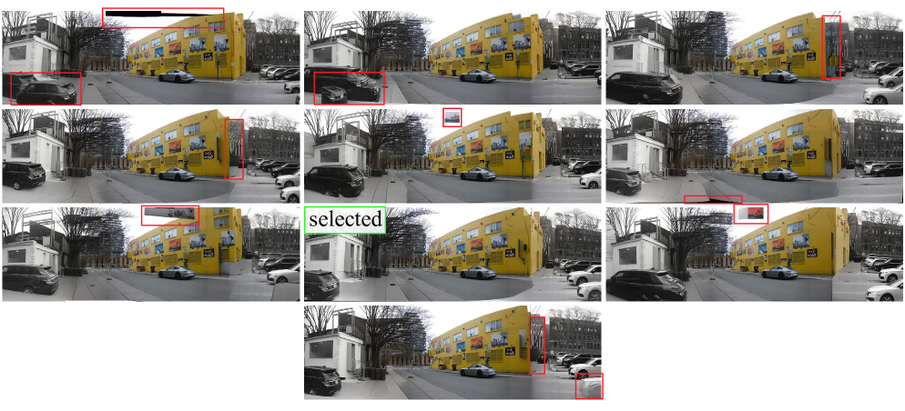
Figure S5: Example of the correspondence-based seed selection strategy to generate the full panoramic canvas. We generate 10 panoramas with different seeds and select the one with most feature matches. The selected panorama has the least artifacts in this example and is the most seamless and similar to the reference.

S2 Supplementary Results

S2.1 Tripod-Captured Dataset

We show the additional 5 scenes for the tripod-captured dataset in Figure S6. Similar to before, we observe that the Stable Diffusion inpainting model [stablediffusioninpaint] produces image content that is locally plausible, but fails to adhere to the layout and content of the actual scene. Similar to previous scenes, RealFill [tang2024realfill] improves on this result, but tends to repeat scene content and ignores scene layout. Our approach provides a much closer match to the layout provided by the reference panorama.

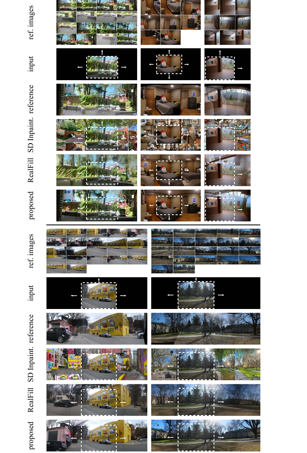
Figure S6: Qualitative results on the additional scenes from the tripod-captured dataset. We find that our approach produces panoramas that are more consistent with the layout and content of the reference panorama than baseline approaches based on inpainting/outpainting.

S2.2 Casually Captured Dataset

We show the additional three scenes for the casually captured dataset in Figure S7. Similar to other scenes, AutoStitch [brown2007automatic], fails to convincingly blend between the different image regions, resulting in ghosting and other artifacts. RealFill exhibits similar artifacts as in the tripod-captured dataset, and we find that our approach produces seamless results that are more consistent with the layout and content of the scene.

Figure S7: Qualitative results of the additional three scenes on the casually captured dataset. Even in this challenging scenario, where the input images have strong parallax effects and variations in style, illumination, color palette, or camera capture settings, our approach reconstructs seamless panoramas that preserve the content and layout of the reference.

S2.3 Supplementary Ablation Studies

Quantitative results.

We conduct an ablation study on the casually captured dataset (see Table S1). We evaluate (1) the effects of parameter choices in positional encoding frequencies (number of channels, max frequency, and omitting token positional encodings), (2) inference strategies, omitting the reference image during inference and denoising tiles row-by-row, with rows sorted by distance to the starting image in the y-axis, and tiles sorted by the distance to the centroid in the x-axis, (3) various guidance scales, (4) various overlap ratios, and (5) training without positional encoding and only using warped reference images. Each ablation uses correspondence-based seed selection to eliminate concerns over seed selection.

Significantly lower max frequency (10Hz), smaller number of channels (4 channels), and no token positional encoding show improvements in some image quality metrics, but a fall in the feature-matching-based metrics. The higher frequencies of the proposed method (12-channels, 50Hz) allow for finer details and better reconstruction of features from the reference images.

Removing the reference image shows a drop across the board in performance, showing the necessity of a starting reference image, as expected. Performance still outperforms prior baselines (see Table LABEL:tab:casual).

Guidance scales between $1.5$ and $2.00$ and overlap ratios between $0.1$ and $0.2$ show the best performance in class. We chose a guidance scale of $1.5$ with an overlap ratio of $0.2$. Generating panoramas using a row-by-row sorting shows marginal improvements in some metrics, however, we found qualitatively that more artifacts are produced. These artifacts are more evident to users, and therefore we opted not to use this strategy.

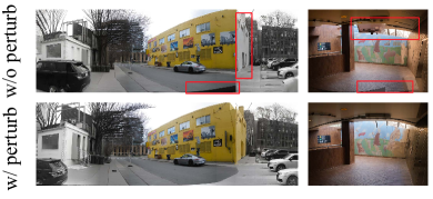
Figure S8: Qualitative evaluation of the ablation omitting the similarity transform used to perturb the location of the warped images in the sparse panoramas.

RealFill with warped reference images suffers from similar repetitive content and a lack of adhesion to the reference layout, demonstrating the need for our proposed positional encoding conditioning.

Method	PSNR $\uparrow$	SSIM $\uparrow$	LPIPS $\downarrow$	DreamSim $\downarrow$	DINO $\uparrow$	CLIP $\uparrow$	LoFTR (L2 Distance) $\downarrow$	LoFTR (Matching) $\uparrow$
proposed (10Hz)	11.09 (2.03)	0.414 (0.100)	0.532 (0.065)	0.137 (0.024)	0.971 (0.011)	0.917 (0.034)	21.65 (4.48)	0.119 (0.037)
proposed (4 channels)	11.12 (1.96)	0.416 (0.102)	0.543 (0.065)	0.134 (0.013)	0.973 (0.011)	0.914 (0.042)	21.95 (5.54)	0.109 (0.039)
proposed (w/o token pos enc)	10.99 (2.29)	0.413 (0.104)	0.544 (0.068)	0.149 (0.033)	0.975 (0.009)	0.913 (0.037)	19.89 (3.82)	0.114 (0.044)
proposed (no ref)	10.20 (2.04)	0.311 (0.138)	0.666 (0.067)	0.235 (0.065)	0.943 (0.011)	0.866 (0.047)	26.89 (6.25)	0.107 (0.042)
proposed (guidance=0.99)	12.22 (1.92)	0.395 (0.140)	0.508 (0.061)	0.154 (0.032)	0.972 (0.011)	0.922 (0.043)	18.13 (4.57)	0.118 (0.057)
proposed (guidance=1.00)	12.22 (1.92)	0.395 (0.140)	0.508 (0.061)	0.154 (0.032)	0.972 (0.011)	0.922 (0.043)	18.13 (4.57)	0.118 (0.057)
proposed (guidance=2.00)	11.07 (2.25)	0.363 (0.135)	0.514 (0.073)	0.145 (0.044)	0.972 (0.012)	0.922 (0.038)	17.20 (4.32)	0.131 (0.056)
proposed (guidance=3.00)	10.43 (2.28)	0.348 (0.129)	0.539 (0.073)	0.165 (0.042)	0.968 (0.013)	0.919 (0.032)	16.91 (5.64)	0.122 (0.058)
proposed (guidance=5.00)	9.57 (2.14)	0.330 (0.125)	0.593 (0.066)	0.188 (0.041)	0.962 (0.018)	0.917 (0.035)	17.79 (6.15)	0.109 (0.055)
proposed (guidance=7.50)	8.80 (1.50)	0.310 (0.107)	0.648 (0.049)	0.251 (0.065)	0.940 (0.034)	0.897 (0.040)	24.03 (15.30)	0.097 (0.056)
proposed (overlap=0.00)	11.37 (2.18)	0.373 (0.144)	0.514 (0.079)	0.136 (0.031)	0.974 (0.009)	0.919 (0.035)	17.82 (5.25)	0.124 (0.052)
proposed (overlap=0.10)	11.34 (1.89)	0.372 (0.137)	0.507 (0.077)	0.140 (0.033)	0.970 (0.012)	0.920 (0.030)	16.52 (5.02)	0.128 (0.053)
proposed (overlap=0.50)	11.56 (2.11)	0.377 (0.140)	0.501 (0.082)	0.135 (0.040)	0.970 (0.010)	0.927 (0.029)	19.20 (7.96)	0.128 (0.055)
proposed (overlap=0.75)	11.71 (2.06)	0.378 (0.133)	0.499 (0.084)	0.135 (0.038)	0.971 (0.013)	0.932 (0.022)	18.43 (9.01)	0.119 (0.062)
proposed (row-by-row)	11.54 (2.16)	0.379 (0.142)	0.507 (0.070)	0.131 (0.026)	0.974 (0.011)	0.911 (0.045)	17.75 (4.98)	0.129 (0.051)
RealFill (warped ref)	10.39 (1.64)	0.309 (0.132)	0.667 (0.080)	0.248 (0.040)	0.932 (0.020)	0.884 (0.024)	60.56 (26.77)	0.016 (0.002)
proposed	11.35 (2.15)	0.374 (0.143)	0.508 (0.076)	0.137 (0.033)	0.971 (0.013)	0.917 (0.035)	17.97 (5.14)

Table S1: Ablation study. We evaluate the effects of (1) using a max frequency of 10Hz for the positional encoding (10Hz), (2) using 4 channels for the positional encoding (4 channels), (3) omitting the token positional encoding in the positional encoding (w/o token pos enc), (4) omitting the reference image during inference (no ref), (5) various guidance scales (guidance), (6) various overlap ratios (overlap), (7) tiling strategy, denoising row-by-row (row-by-row), and (8) RealFill trained with the warped reference images. We compare the generated results to a reference panorama produced using AutoStitch [brown2007automatic] on the tripod-captured dataset as in the main paper.

Qualitative results.

We show qualitative results for the effect of perturbing the locations of sparse images in the panorama Figure S8. Without perturbation, the model is less robust to misalignments in the initial layout estimation.

We show qualitative results for the various guidance scales in Figure S9. Lower guidance scales ($<1.5$) maintain scene quality but fail to properly blend through artifacts (e.g. building remains grayscale). Guidance scales between $1.5-2$ show how scene cohesion can be maintained while also resolving artifacts found in the reference images (building is well blended). Higher guidances begin to exhibit “cartoonish” effects and the scene loses cohesion (obvious seams between regions in the panorama).

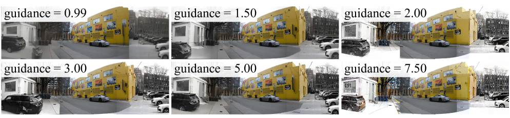
Figure S9: Qualitative comparison of various guidance scales on the casually-captured dataset. We find that increasing guidance leads to more “cartoonish” outputs and more seams, with a guidance scale around $1.5$ showing best results.