Ampere: Communication-Efficient and High-Accuracy Split Federated Learning

Abstract

A Federated Learning (FL) system collaboratively trains neural networks across devices and a server but is limited by significant on-device computation costs. Split Federated Learning (SFL) systems mitigate this by offloading a block of layers of the network from the device to a server. However, in doing so, it introduces large communication overheads due to frequent exchanges of intermediate activations and gradients between devices and the server and reduces model accuracy for non-IID data. We propose Ampere, a novel collaborative training system that simultaneously minimizes on-device computation and device-server communication while improving model accuracy. Unlike SFL, which uses a global loss by iterative end-to-end training, Ampere develops unidirectional inter-block training to sequentially train the device and server block with a local loss, eliminating the transfer of gradients. A lightweight auxiliary network generation method decouples training between the device and server, reducing frequent intermediate exchanges to a single transfer, which significantly reduces the communication overhead. Ampere mitigates the impact of data heterogeneity by consolidating activations generated by the trained device block to train the server block, in contrast to SFL, which trains on device-specific, non-IID activations. Extensive experiments on multiple CNNs and transformers show that, compared to state-of-the-art SFL baseline systems, Ampere (i) improves model accuracy by up to 13.26% while reducing training time by up to 94.6%, (ii) reduces device-server communication overhead by up to 99.1% and on-device computation by up to 93.13%, and (iii) reduces standard deviation of accuracy by 53.39% for various non-IID degrees highlighting superior performance when faced with heterogeneous data.

1 Introduction

A federated learning (FL) [1, 2, 3, 4] system is a distributed system that enables multiple devices to collaboratively train a deep neural network (DNN), such as convolutional neural networks (CNN) and transformers, without sharing their original input data. Each device trains a model locally in FL and periodically sends it to the server for aggregation. However, training a complete DNN on end-user devices with relatively limited computing and memory resources, such as smartphones or tablets, presents significant challenges. These devices typically have limited GPU capabilities, making the training of even medium-sized DNNs prohibitively slow. Additionally, limited RAM/VRAM on these devices often prevents them from holding both the model parameters and training data in memory.

Split Federated Learning (SFL) [5] systems reduce the computational workload on devices in FL by offloading part of the model training to a server with more computational resources. In an SFL system, the model is divided into a device block and a server block. The device block processes inputs locally and sends intermediate activations to the server, which computes the loss. The server block then returns the gradients of the activations to the device (Figure 1(a)).

Large communication overhead: While SFL systems reduce on-device computation, they introduce communication in addition to the periodic model transfers in FL. Each training iteration exchanges activations and gradients between the device and server, resulting in frequent, high-volume data transfers (red arrows in Figure 1(a)). In bandwidth-limited environments, this overhead severely impacts efficiency, making SFL systems impractical for real-world deployments (see Challenge 1 and Challenge 2 discussed further in Section 2.2).

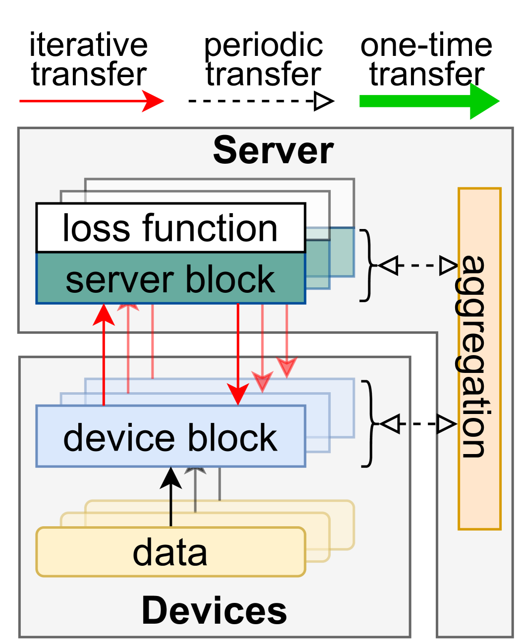
(a) Split Federated Learning

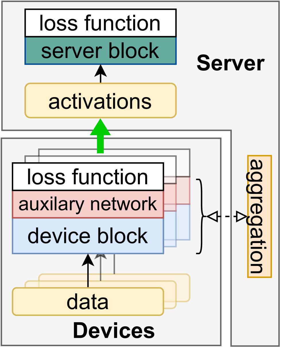
(b) Ampere

Figure 1: Training in a Split Federated Learning (SFL) system and Ampere. SFL exchanges activations and gradients in each iteration; Ampere only transfers activations once.

Several methods have been proposed to reduce the communication overhead in SFL systems, such as compressing activations and gradients [6, 7, 8, 9, 10], overlapping communication and computation [11], and computing local gradients [12, 13] (discussed further in Section 6). However, these methods still require transferring activations each iteration, preventing them from achieving the communication efficiency of classic FL.

To address the above limitation, we propose Ampere (Figure 1(b)), a novel system that eliminates iterative activation and gradient transfers in SFL by developing unidirectional inter-block training (see Section 3.2.1). Instead of exchanging activations and gradients at each iteration, Ampere first trains the device block to convergence using a lightweight auxiliary network (see Section 3.2.2) to compute local loss without needing gradients from the server. Once the device block is trained, activations are transferred to the server once, allowing the server block to be trained independently. The primary communication overhead of SFL arises from iterative activation and gradient transfers, but Ampere changes this to a single activation transfer (green arrows in Figure 1(a); no gradients are transferred from the server). Communication in Ampere is reduced to the exchanges of device blocks for aggregation, which has an even lower communication overhead than classic FL.

Degraded accuracy due to data heterogeneity: In addition to communication overhead, SFL systems inherit non-independent and identically distributed (non-IID) data-related problems from FL. Given heterogeneous data each device will have a different data distribution in FL, leading to model divergence and reduced accuracy. These problems persist in SFL as non-IID data on devices generates skewed activations that negatively impact the training of the server block. While existing FL methods mitigate non-IID problems to some extent using modified aggregation strategies and objective functions [14, 15, 16], they are less effective in SFL. To address this, Ampere leverages the split architecture to merge device activations into a single, more homogeneous dataset for server block training. This activation consolidation method (see Section 3.2.3) ensures that the server block trains on more IID inputs, which in turn improves the overall model accuracy.

Figure 2: Trade-off between on-device computation and device-server communication for Federated Learning (FL), Split Federated Learning (SFL), and Ampere. FL and SFL have similar accuracy whereas Ampere has a higher accuracy than these methods.

As shown in Figure 2, Ampere is the first system to simultaneously (i) reduce communication overhead to FL levels while achieving low on-device computation as in SFL, and (ii) improve model accuracy on non-IID data, surpassing both FL and SFL. Extensive experimental evaluations conducted on various DNNs and non-IID datasets demonstrate that, compared to state-of-the-art SFL baselines, Ampere reduces communication overhead by up to 99.1% and on-device computation by up to 93.13%, reduces training time by up to 94.6%, and improves model accuracy by up to 13.26%. In addition, Ampere reduces the standard deviation of accuracy for various non-IID degrees by up to 53.39% compared to other baselines, demonstrating that it is less impacted by non-IID data.

The key research contributions of this paper are as follows:

1. Ampere, a novel system that is underpinned by unidirectional inter-block training, a new method to significantly reduce both communication and computation overhead while simultaneously improving model accuracy compared to FL/SFL.

2. A new method to generate a lightweight auxiliary network that breaks the interdependency between the device and server blocks during training, eliminating the iterative transfer of intermediate results.

3. An efficient activation consolidation and management strategy to reduce activation heterogeneity is demonstrated to improve model accuracy.

The rest of this paper is organized as follows. Section 2 introduces SFL and identifies three opportunities to address critical challenges in SFL. Section 3 presents Ampere and describes its underlying methods. Section 4 analyzes model convergence and communication costs of Ampere. Section 5 evaluates Ampere against relevant baselines. Section 6 discusses the related work, and Section 7 concludes the paper.

2 Background

In this section, we present split federated learning (SFL), identify three key challenges that limit its adoption in the real-world, and present opportunities in collaborative learning beyond SFL.

2.1 Split Federated Learning

In a classic FL system, training the complete neural network $\theta$ on devices is prohibitively expensive (computation and memory usage) on end-user devices.

Split Federated Learning (SFL) [5] systems address these constraints by splitting the model into two blocks – a device block $\theta^{(d)}$ and a server block $\theta^{(s)}$ that is offloaded to the server. Suppose $K$ devices participate in training; each device $k\in[K]$ has its own dataset $\mathcal{D}_{k}=\left\{(x_{i},y_{i})\right\}_{j=1}^{n_{k}}$, with $x_{i}$ denoting an input sample, $y_{i}$ its label, and $n_{k}=|\mathcal{D}_{k}|$. The overall objective is to train a global model $\theta=(\theta^{(d)},\theta^{(s)})$ that minimizes the following objective function:

$$\min_{\theta}F\left(\theta\right)=\sum_{k=1}^{K}\frac{n_{k}}{n}F_{k}\left(\theta^{(d)},\theta^{(s)}\right)$$ (1)

where $n=\sum_{k=1}^{K}n_{k}$ is the total number of data samples across all devices. For a given device $k$, its local loss function $F_{k}$ is defined as:

$$F_{k}\left(\theta^{(d)},\theta^{(s)}\right)=\frac{1}{n_{k}}\sum_{i=1}^{n_{k}}f^{(s)}\left(\theta^{(s)}_{k};f^{(d)}\left(\theta^{(d)}_{k};x_{i}\right),y_{i}\right)$$ (2)

where $f^{(d)}\left(\theta^{(d)}_{k};x_{i}\right)$ denotes the device-side forward function, and $f^{(s)}\left(w^{(s)}_{k};*\right)$ is the server-side loss function that computes the prediction error with respect to the label $y_{i}$.

Forward and backward passes in SFL: During local training on device $k$, the device block $\theta^{(d)}_{k}$ processes $x_{i}$ to produce activations $\xi_{i}=f^{(d)}\left(\theta^{(d)}_{k};x_{i}\right)$, which are sent to the server. The server block $\theta^{(s)}_{k}$ completes the forward pass and computes the loss. In the backward pass, gradients of $\theta^{(s)}_{k}$ are obtained and used to update it. Simultaneously, the server sends the corresponding gradients of $\xi$ back to the device, enabling the backward pass of $\theta^{(s)}_{k}$. $\theta^{(d)}_{k}$ and $\theta^{(s)}_{k}$ are updated using stochastic gradient descent (SGD):

$$\theta^{(d)}_{k}\leftarrow\theta^{(d)}_{k}-\eta\nabla F_{k}\left(\theta^{(d)}_{k}\right),\enspace\theta^{(s)}_{k}\leftarrow\theta^{(s)}_{k}-\eta\nabla F_{k}\left(\theta^{(s)}_{k}\right)$$ (3)

where $\eta$ is the learning rate. Exchanging activations $\xi_{i}$ and their gradients in each training iteration adds substantial device-server communication overhead beyond classic FL.

Model aggregation: After a user-defined number of local iterations, each device sends its updated $\theta^{(d)}_{k}$ to the server. The server then aggregates these updates into $\theta^{(d)}$ using the FedAvg algorithm [1]; meanwhile, the server blocks are aggregated into $\theta^{(s)}$:

$$\theta^{(d)}\leftarrow\sum_{k=1}^{K}\frac{n_{k}}{n}\,\theta^{(d)}_{k},\enspace\theta^{(s)}\leftarrow\sum_{k=1}^{K}\frac{n_{k}}{n}\,\theta^{(s)}_{k}$$ (4)

Finally, the server broadcasts the updated $\theta^{(d)}$ to all devices for the next round of local training. This process is repeated until convergence. The non-IID nature of the data locally generated on devices $\{D_{k}\}$ reduces model accuracy compared to training on a centralized dataset $\bigcup\limits_{k=1}^{K}D_{k}$.

2.2 Opportunities Beyond SFL Systems

Although SFL systems reduce on-device computation, they face three critical challenges due to additional communication (Challenge 1 and Challenge 2) and data heterogeneity (Challenge 3), which limit their adoption in practice.

2.2.1 Challenge 1: Trade-Off between On-device Computation and Device-Server Communication

Selecting the optimal layer at which the network must be split, referred to as split point, is crucial as it impacts both on-device computation and device-server communication. To illustrate this a MobileNetV3-Large (MobileNet-L) [17] model is trained on the CIFAR-10 [18, 19] dataset (Figure 3). The experimental setup is presented in Section 5.1. On-device computation (measured in GFLOPS) and device-server communication volume (shown in GB), including model parameters and intermediate results (activations and gradients), are measured for various split points. Lower split points offload more layers to the server and reduce on-device computation. However, earlier layers generate larger intermediate results, increasing the communication overhead. For example, when compared to classic FL (when all 19 layers are on the device), splitting the network after the first layer reduces on-device computation by 98.21%, but increases communication by 9.63$\times$.

Figure 3: Trade-off between communication volume and on-device computation per round of MobileNet-Large using an SFL system for different split points.

2.2.2 Challenge 2: High Device-Server Communication Volume and Frequency

The split point in SFL is usually selected at the early layers of the model to ensure that the device block remains lightweight and can be trained efficiently on resource-constrained devices [20, 11]. However, this leads to a significant increase in the communication volume compared to FL, as large intermediate activations must be transferred from devices to the server during each iteration.

Additionally, end-to-end training of the device and server blocks is tightly interdependent, as the device block relies on the global loss function computed on the server. This leads to a high communication frequency that cannot be reduced, making SFL impractical in bandwidth-constrained environments.

We compare the communication volume and frequency for training a MobileNet-L model on CIFAR-10 using FL and SFL with a split point at the first layer. Both methods train for 150 epochs until convergence. Each time a model or a batch of activations/gradients is transferred, it is counted as a communication round. As shown in Table I, SFL increases the total communication volume by one order of magnitude and the communication frequency by three orders of magnitude compared to FL.

TABLE I: Communication volume and frequency in FL and SFL for MobileNet-L.

System	Communication volume (GB)	Communication rounds per hour
FL	57	768
SFL	549	3578280

2.2.3 Challenge 3: Data Heterogeneity Reduces Model Accuracy

In classic FL, each device’s dataset is typically non-independent and non-identically distributed (non-IID), causing local models to learn device-specific patterns that do not generalize well when aggregated. This reduces the accuracy of the global model compared to training on IID data.

In SFL, each device processes non-IID data, generating skewed activations. The server typically trains multiple server blocks, each on activations from a single device. Similar to device blocks, the server blocks are aggregated periodically. As a result, server blocks learn from skewed activations that represent feature abstractions of the non-IID input data, reducing model accuracy. As data heterogeneity increases and more devices participate, the activation is skewed more, which further degrades accuracy.

Figure 4: Model accuracy of MobileNet-Large for varying number of devices and non-IID degree $\alpha$.

Data heterogeneity is modeled using the CIFAR-10 dataset, where the data is partitioned across multiple devices following a Dirichlet distribution $Dir(\frac{\alpha}{1-\alpha+\epsilon})$ (see Section 5.1). A smaller $\alpha$ results in a higher non-IID degree, whereas $\alpha=1$ approximates an IID scenario. Figure 4 shows that model accuracy decreases when $\alpha$ gets smaller because the data on individual devices becomes more heterogeneous. Additionally, for a given $\alpha$, increasing the number of devices further amplifies heterogeneity and reduces accuracy. The dashed line in the figure shows the accuracy achieved when training on the entire dataset (which is IID), serving as an upper bound for model accuracy under any non-IID configuration.

3 Ampere

In this section, we leverage the three opportunities identified in the previous section to design a new system Ampere. Three new methods, namely unidirectional inter-block training, lightweight auxiliary network generation, and efficient activation consolidation are developed and incorporated in Ampere. The training algorithm incorporating these methods is also considered.

3.1 Overview

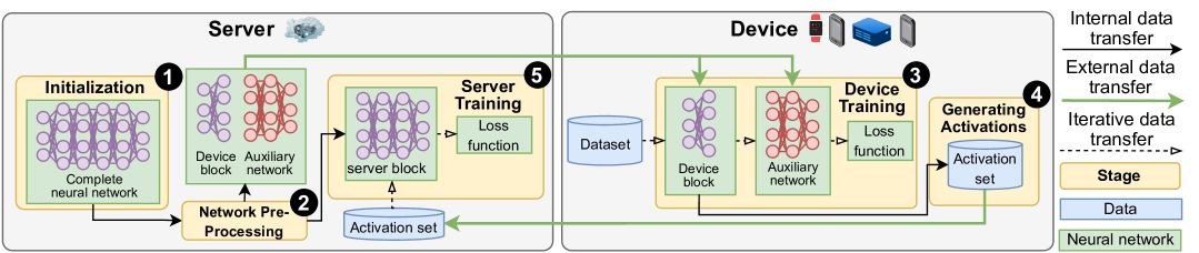
Figure 5: Overview of Ampere.

Ampere operates with a single server and $K$ devices, collaboratively training a deep neural network $\theta$ via unidirectional inter-block training (UIT) instead of training based on conventional end-to-end backpropagation. Specifically, Ampere splits $\theta$ into a device block and a server block, first training the device block until convergence before proceeding to train the server block. This process follows five key steps (see Figure 5):

Step : Initialization - the server initializes the complete neural network $\theta$.

Step : Network Pre-processing - $\theta$ is split into two blocks: (i) Device block $\theta^{(d)}$, comprising the initial layers of $\theta$. (ii) Server block $\theta^{(s)}$, containing the remaining layers. An auxiliary network $\tilde{\theta}^{(d)}$ is generated to connect the outputs of $\theta^{(d)}$ to a local loss function. The server then transfers $\theta^{(d)}$ and $\tilde{\theta}^{(d)}$ to all participating devices, denoted as $\theta^{(d)}_{k}$ and $\tilde{\theta}^{(d)}_{k}$ for device $k$.

Step : Device Training - devices train $\left\{\theta^{(d)}_{k},\tilde{\theta}^{(d)}_{k}\right\}$ locally until convergence using the auxiliary network and local loss function. Unlike SFL, gradients of device blocks are computed locally in Ampere without sending intermediate activations to the server.

Step : Generating Activations - each device generates activations by feeding local data into its trained device block $\theta^{(d)}$. These activations are transferred once to the server, where they are consolidated for training the server block.

Step : Server Training - $\theta^{(s)}$ is trained on the server using the consolidated activations, without interacting with devices.

The above sequential steps execute only once, eliminating the iterative back-and-forth device-server communication in SFL.

3.2 Methods

The three methods developed in Ampere are presented.

3.2.1 Unidirectional Inter-Block Training to Eliminate the On-device Computation and Device-server Communication Trade-off

Classic SFL relies on end-to-end backpropagation (BP)-based training. In each training iteration, data is transferred from the device block to the server block during the forward pass, while gradients propagate back during the backward pass. This results in a fundamental trade-off between on-device computation and device-server communication, which cannot be simultaneously optimized at the same split point as presented in Section 2.2.1.

In contrast, Ampere develops unidirectional inter-block training (UIT), treating the device block and the server block as independent modules trained sequentially rather than iteratively. UIT transfers activations from the device to the server only once during training and no gradients are sent from the server to the device. This approach eliminates the aforementioned trade-off by ensuring that on-device computation and device-server communication are optimized simultaneously at the same split point.

Split point $p$ refers to the number of layers in the device block. Similar to BP, on-device computation in UIT increases with the number of layers in the device block $\theta^{(d)}$ (increasing $p$). Thus, placing only the first layer on the device ($p=1$) reduces computation.

However, the trend of UIT communication with respect to the split point in Ampere differs from BP. UIT communication consists of: (i) Model exchanges for aggregating device blocks in Step  . (ii) A one-time activation transfer in Step  .

We measure the parameter size $s^{l}_{i}$ and output (activation) size $s^{o}_{i}$ for each layer $i\in[1,I]$, where $I$ is the total number of layers. The total communication volume $C$ over $N$ training epochs is:

$$C=2N\sum_{i=1}^{p}s^{l}_{i}+s^{o}_{p}$$ (5)

where the first term accounts for model exchanges occurring twice per epoch, while the second term represents the one-time activation transfer. Since training typically requires $N\geq 100$ epochs, the activation transfer cost $s^{o}_{p}$ becomes negligible (see Section 4.2 for a detailed analysis), and $C$ is dictated by $\sum_{i=1}^{p}s^{l}_{i}$, which increases with $p$. Thus, $p=1$ minimizes the device-server communication.

Figure 6 shows the communication volume and on-device computation per training round for MobileNet-Large on CIFAR-10. For BP the lowest amount of on-device computation and device-server communication incurred are achieved at different split points, $p=1$ and $p=14$, respectively. In contrast, UIT demonstrates a consistent trend – both increase with $p$. As a result, the optimal split point $p_{opt}=1$ of UIT simultaneously minimizes both computation and communication, thereby addressing Challenge 1.

Figure 6: Communication volume and on-device computation per training round for MobileNet-Large using BP and UIT for different split points.

3.2.2 Lightweight Auxiliary Network Generation to Break Iterative Dependency Between Device and Server Training

When using BP in SFL, the device and server blocks are optimized using a global loss function. This is the primary reason for the tight interdependency between the device and server due to frequent iterative transfers of activations and gradients. A large communication volume and frequency is the resultant as highlighted in Section 2.2.2.

To break this dependency, Ampere introduces a method to generate an auxiliary network $\tilde{\theta}^{(d)}$ that enables independent training of $\theta^{(d)}$. This network connects $\theta^{(d)}$ to a local loss function, allowing devices to compute gradients without requiring gradients from the server.

Since $\tilde{\theta}^{(d)}$ runs on resource-constrained devices, it must be lightweight to keep the computational overhead low while capturing meaningful feature representations for training the server block. To achieve this, a compact two-layer design is followed. The first layer replicates the first layer in $\theta^{(s)}$ but halves the dimension. The second layer is a fully connected layer with the same loss function as in $\theta^{(s)}$.

The second layer of $\tilde{\theta}^{(d)}$ provides a direct mapping to the loss function so that local training is feasible. The first layer ensures $\theta^{(d)}$ captures generalizable features from raw data, which is essential for the effective learning of the subsequent layers in the server block [21]. Without this layer, $\tilde{\theta}^{(d)}$ would rely on a fully connected layer, forcing $\theta^{(d)}$ to extract task-specific abstract representations. However, since activations are shallow representations for server block training, such features do not generalize well across devices and degrade overall model performance [22, 23].

The dimension of both layers in $\tilde{\theta}^{(d)}$ impacts both model accuracy and computational cost. The method that generates the auxiliary network aims to reduce on-device computation, for which the auxiliary network’s dimension is scaled down relative to the first layer of the server block. Figure 7 empirically demonstrates the effect of different dimension ratios of the auxiliary network relative to the first layer of the server block on MobileNet-Large trained on CIFAR-10. As the dimension ratio increases from 0.25 to 1.0, computational overhead grows linearly, while accuracy improvements become marginal beyond 0.5. Therefore, 0.5 is the selected ratio in Ampere but allows users to adjust it.

Figure 7: Impact of varying auxiliary network dimensions on on-device computation per round and final model accuracy. The x-axis represents the dimension ratio of auxiliary network relative to the first layer of the server block.

By decoupling device and server training using this lightweight auxiliary network, Ampere reduces iterative activation transfers to a one-shot transfer, significantly minimizing communication overhead and addressing Challenge 2.

3.2.3 Activation Consolidation to Mitigate Impact of Data Heterogeneity

Ampere for the first time addresses activation heterogeneity when collaboratively training multiple devices by introducing activation consolidation on the server. Unlike SFL systems, where the server block is trained on the activations generated from non-IID local data across devices, Ampere trains the server block on the activations produced by a converged and consistent device block using data from all devices. This mitigates the heterogeneity of activations and improves model accuracy.

In a typical SFL system, each device $k$ generates activations from its local dataset $\mathcal{D}_{k}$, leading to skewed intermediate feature representations across different devices. When the server trains $K$ separate server blocks, each on the activations from a single device, the non-IID activation distributions lead to inconsistent feature learning across server blocks, reducing generalization and overall model accuracy. SplitFedV2, a variant of SplitFed [5], removes server-side model aggregation by training a single server block. However, the server block is still trained on activations uploaded in every training iteration, although the device blocks are often not fully trained. As the parameters of the device blocks continue to change during each training iteration, the resulting activations for the same input will also change. This adversely impacts the server block’s accuracy.

To mitigate the impact of activation heterogeneity, Ampere takes a fundamentally different approach by performing one-shot activation consolidation after the convergence of the device block. Each device generates activations using the same converged device block and uploads them once to the server. The server then forms a unified activation set $\mathcal{A}$:

$$\mathcal{A}=\left\{\left(\xi_{i},y_{i}\right);\xi_{i}=f^{d}\left(\theta^{(d)};x_{i}\in\bigcup\limits_{k=1}^{K}\mathcal{D}_{k}\right)\right\}$$ (6)

where $\xi_{i}$ represents the activation generated from input $x_{i}$ by the converged device block $f^{d}(\theta^{(d)})$, and $y_{i}$ is its label. Subsequently, a single server block is trained on the unified activation set $\mathcal{A}$.

This approach reduces activation heterogeneity and improves server-side generalization over existing SFL systems for two reasons. First, since all activations are generated using the same converged device block, the representation mapping is identical across devices. This eliminates inconsistencies that would otherwise arise from model parameter variations. Second, by consolidating activations from all devices, the unified activation set $\mathcal{A}$ better approximates the global data distribution. This improves the diversity and balance of the training set seen by the server block, enabling it to learn more generalizable representations.

3.3 Training Algorithm

Training in Ampere follows a dual-step approach (as shown in Algorithm 1): (1) the device block is trained, similar to FL, alongside an additional auxiliary network, and (2) the server trains a single server block in a centralized manner.

Device Training: The device block $\theta^{(d)}$ is trained locally with the auxiliary network $\tilde{\theta}^{(d)}$. On each device $k$, $\theta^{(d)}$ and $\tilde{\theta^{(d)}}$ are trained iteratively, minimizing the objective:

$$\min_{\theta^{(d)}}F^{(d)}(\theta^{(d)})=\sum_{k=1}^{K}\frac{n_{k}}{n}F^{(d)}_{k}(\theta^{(d)},\tilde{\theta}^{(d)})$$ (7)

where $F^{(d)}_{k}$ is the local loss function on device $k$:

$$F^{(d)}_{k}\left(\theta^{(d)},\tilde{\theta}^{(d)}\right)=\frac{1}{n_{k}}\sum_{i=1}^{n_{k}}\tilde{f}^{(d)}\left(\tilde{\theta}^{(d)}_{k};f^{(d)}\left(\theta^{(d)}_{k};x_{i}\right),y_{i}\right)$$ (8)

Each iteration involves sampling a mini-batch from the local dataset (Line 4) and computing activations $\xi_{i}$ via the feed-forward function $f^{(d)}$. The auxiliary network $\tilde{f}^{(d)}$ then computes the local loss and updates $\theta^{(d)}$ and $\tilde{\theta}^{(d)}$ (Line 5):

$$\begin{split}\theta^{(d)}_{k}\leftarrow\theta^{(d)}_{k}-\eta^{(d)}\nabla F^{(d)}_{k}\left(\theta^{(d)}_{k}\right)\\ \tilde{\theta}^{(d)}_{k}\leftarrow\tilde{\theta}^{(d)}_{k}-\eta^{(d)}\nabla F^{(d)}_{k}\left(\tilde{\theta}^{(d)}_{k}\right)\end{split}$$ (9)

where $\eta^{(d)}$ is the learning rate of the device block.

The updated local models are then sent to the server (Line 6) and aggregated using (Lines 13-14):

$$\theta^{(d)}\leftarrow\sum_{k=1}^{K}\frac{n_{k}}{n}\theta^{(d)}_{k},\enspace\tilde{\theta}^{(d)}\leftarrow\sum_{k=1}^{K}\frac{n_{k}}{n}\tilde{\theta}^{(d)}_{k}$$ (10)

The global model is then sent to the devices (Line 15) and update the local models (Line 8). This process repeats until $\left\{\theta^{(d)},\tilde{\theta^{(d)}}\right\}$ converges or reaches $N^{(d)}$ epochs.

Activation Transfer: Once device block training completes, each device generates activations by feeding local data into $\theta^{(d)}$ and sends them with their labels to the server (Line 10), consolidating an activation set $\mathcal{A}$ (Equation 6).

Server Training: The server performs two tasks: (i) storing activations from the devices on disk (Line 16) and (ii) loading activation batches for training the server block (Lines 17-19). Since devices send activations at different rates, waiting for all activations before training the server block introduces idle time. To mitigate this, these tasks run asynchronously in parallel, allowing training to begin as soon as the first batch of activations is available, improving training efficiency.

The server block $\theta^{(s)}$ is trained on the consolidated activation set to optimize the following objective:

$$\min_{\theta^{(s)}}F^{(s)}\left(\theta^{(s)}\right)=\frac{1}{|\mathcal{A}|}\sum_{i=1}^{|\mathcal{A}|}f^{(s)}\left(\theta^{(s)};\xi_{i},y_{i}\right)$$ (11)

where $f^{(s)}$ is the loss function on server. $\theta^{(s)}$ is updated via:

$$\theta^{(s)}\leftarrow\theta^{(s)}-\eta^{(s)}\nabla F^{(s)}\left(\theta^{(s)}\right)$$ (12)

where $\eta^{(s)}$ is the learning rate of the server block. Training continues until convergence or reaches $N^{(s)}$ epochs.

1

2

/* Training device blocks in parallel */

3 Function DeviceTraining($k$, $\mathcal{D}_{k}$, $N^{(d)}$, $B^{(d)}$):

    Input: device index $k\in[K]$, dataset $\mathcal{D}_{k}$, #device epochs $N^{(d)}$, #iterations per epoch $H$, batch size $B^{(d)}$

    Output: trained device block $\theta^{(d)}$

4   

5   for $n\leftarrow 0$ to $N^{(d)}$ do

6       for $h\leftarrow 0$ to $H$ do

7          Sample mini-batch $\left\{\bm{x}_{h},\bm{y}_{h}\right\}\in\mathcal{D}_{k}$ of size $B^{(d)}$

8         Update $\theta^{(d)}_{k}$ and $\tilde{\theta}^{(d)}_{k}$ (Equation 9)

9      Send $\left\{\theta^{(d)}_{k},\tilde{\theta}^{(d)}_{k}\right\}$ to server

10      Receive global models $\left\{\theta^{(d)},\tilde{\theta}^{(d)}\right\}$

11      Update local models: $\left\{\theta^{(d)}_{k},\tilde{\theta}^{(d)}_{k}\right\}\leftarrow\left\{\theta^{(d)},\tilde{\theta}^{(d)}\right\}$

12   

   // Send activations for server training

13    foreach $\left\{\bm{x}_{i},\bm{y}_{i}\right\}\in\mathcal{D}_{k}$ do

14       Compute activations $\bm{\xi}_{i}$ (Equation 6) and send to server

15   

16

/* Training the server block */

17 Function ServerTraining($N^{(d)},N^{(s)},B^{(s)},S$):

    Input: #device epochs $N^{(d)}$, #server epochs $N^{(s)}$, batch size $B^{(s)}$, activation size $S$

    Output: trained server block $\theta^{(s)}$

18   

   // Aggregate device blocks

19    for $n\leftarrow 0$ to $N^{(d)}$ do

20       Receive $\left\{\theta^{(d)}_{k},\tilde{\theta}^{(d)}_{k};k\in[K]\right\}$ from devices

21      Aggregate into $\theta^{(d)}$ and $\tilde{\theta}^{(d)}$ (Equation 10)

22      Send $\left\{\theta^{(d)},\tilde{\theta}^{(d)}\right\}$ to devices

23   

   // Subprocess 1: Receive and store activations

24    Run StoreActivation($\left\{\bm{\xi}_{i},\bm{y}_{i}\right\}$)

   // Subprocess 2: Load activations to train the server block

25    for $n\leftarrow 0$ to $N^{(s)}$ do

26       foreach $\left\{\bm{\xi}_{i},\bm{y}_{i}\right\}\in$ LoadActivation() do

27          Update $\theta^{(s)}$ (Equation 12)

28      

29   

Algorithm 1 Training in Ampere

4 Convergence and Communication Cost Analysis

This section analyzes the convergence of Ampere, and demonstrates that Ampere incurs lower communication costs than both FL and SFL.

4.1 Convergence Analysis

The convergence of the device block and server block are analyzed based on the general assumptions of FL and SFL systems.

4.1.1 Notation

The parameters of device blocks and the auxiliary networks are denoted as $\varphi=\left(\theta^{(d)},\,\tilde{\theta}^{(d)}\right)$. $\varphi_{k}^{t}$ denotes the parameters of $t$ iterations on device $k$, where $t\in\left[T^{(d)}\right],T^{(d)}=N^{(d)}H$. The objective of device block training becomes:

$$\min F^{(d)}(\varphi)=\sum_{k=1}^{K}\frac{n_{k}}{n}F^{(d)}_{k}(\varphi)$$ (13)

$F^{(d)}_{k}$ is the local loss function on device $k$, rewritten as:

$$F^{(d)}_{k}\left(\varphi\right)=\frac{1}{n_{k}}\sum_{i=1}^{n_{k}}f(\varphi_{k};x_{i},y_{i})$$ (14)

where

$$f(\varphi_{k};x_{i},y_{i})=\tilde{f}^{(d)}\left(\tilde{\theta}^{(d)}_{k};f^{(d)}\left(\theta^{(d)}_{k};x_{i}\right),y_{i}\right)$$ (15)

We assume the dataset $\mathcal{D}_{k}$ on device $k\in[K]$ follows the distribution $p_{k}(x)$. The non-IID degree is quantified as:

$$\Gamma=F^{(d),*}-\sum_{k=1}^{K}\frac{n_{k}}{n}F^{(d),*}_{k}$$ (16)

where $F^{(d),*}$ and $F^{(d),*}_{k}$ denotes the minimum values of $F^{(d)}$ and $F^{(d)}_{k}$. Larger value of $\Gamma$ indicates a higher degree of non-IID; $\Gamma=0$ indicates IID data.

The distribution of $\xi$ is denoted as $q(\xi)$, where $\xi=f^{d}(x)$. Let $q^{*}(\xi)$ denote the density of the activations from the converged device block. We measure the distance between $q(\xi)$ and $q^{*}(\xi)$ as:

$$c=\int|q(\xi)-q^{*}(\xi)|d\xi$$ (17)

For the sake of simplicity, we use $\theta_{t}$ to denote the parameters of the server block at iteration $t\in\left[T^{(s)}\right]$, replacing $\theta^{(s)}$, where $T^{(s)}=N^{(s)}\lfloor\frac{n}{B^{(s)}}\rfloor$ denotes the total number of iterations of training the server block.

4.1.2 Assumptions

The following general assumptions are made in the literature on FL and SFL systems [24, 25, 26, 27, 28, 29, 30, 31]:

Assumption 1 ($L$-smoothness [24, 26, 27]).

For $\forall k\in[K]$, $F^{(d)}_{k}(\varphi)$ and $F^{(s)}(\theta)$ is $L$-smooth, i.e., $\exists L$, $\forall\varphi,\varphi^{\prime}$, such that

$$\bigl{\|}\nabla F^{(d)}_{k}(\varphi)-\nabla F^{(d)}_{k}(\varphi^{\prime})\bigr{\|}\leq L\bigl{\|}\varphi-\varphi^{\prime}\bigr{\|}$$ (18)

and $\forall\theta,\varphi^{\theta}$, such that

$$\bigl{\|}\nabla F^{(s)}(\theta)-\nabla F^{(s)}(\theta^{\prime})\bigr{\|}\leq L\bigl{\|}\theta-\theta^{\prime}\bigr{\|}$$ (19)

Consequently, $F^{(d)}(\varphi)$ is also $L$-smooth.

Assumption 2 ($\mu$-strong convexity [24]).

For $\forall k\in[K]$, $F^{(d)}_{k}(\varphi)$ is $\mu$-strongly convex, i.e., $\exists\mu$, $\forall\varphi,\varphi^{\prime}$, such that

$$\bigl{\|}\nabla F^{(d)}_{k}(\varphi)-\nabla F^{(d)}_{k}(\varphi^{\prime})\bigr{\|}\geq\mu\bigl{\|}\varphi-\varphi^{\prime}\bigr{\|}$$ (20)

Consequently, $F(\varphi)$ is also $\mu$-strongly convex.

Assumption 3 (Bounded Gradient Variance [24, 28, 29, 30, 31]).

For $\forall k\in[K]$ and $\forall t\in[T^{(d)}]$, the variance of gradients of $F^{(d)}_{k}$ is bounded, i.e., $\forall x\in\mathcal{D}_{k}$, $\exists\sigma_{k}$ such that

$$\mathbb{E}\left[\bigl{\|}\nabla F^{(d)}_{k}(\varphi_{k}^{t};x)-\nabla F^{(d)}_{k}(\varphi_{k}^{t})\bigr{\|}^{2}\right]\leq\sigma_{k}^{2}$$ (21)

Assumption 4 (Bounded Gradient Norm [24, 25, 26, 27, 28, 29, 30, 31]).

For $\forall k\in[K]$ and $\forall t\in[T^{(d)}]$, the expected squared norm of gradients of $F^{(d)}_{k}$ and $F^{(s)}$ is uniformly bounded, i.e., $\forall x\in\mathcal{D}_{k}$, $\exists\sigma_{k}$ such that

$$\mathbb{E}\left[\bigl{\|}\nabla F^{(d)}_{k}(\varphi_{k}^{t};x)\bigr{\|}^{2}\right]\leq G$$ (22)

and

$$\mathbb{E}\left[\bigl{\|}\nabla F^{(s)}(\varphi_{k}^{t};x)\bigr{\|}^{2}\right]\leq G$$ (23)

Assumption 5 (Robbins-Monro Conditions [32, 25, 26, 27]).

The learning rate of the server block $\eta^{(s)}_{t}$ satisfies $\sum_{t}\eta^{(s)}_{t}=\infty$ yet $\sum_{t}\left(\eta^{(s)}_{t}\right)^{2}<\infty$.

4.1.3 Convergence of the device block

Let Assumption 1 to Assumption 4 hold, then we have

Theorem 1 (Device Block Convergence).

If the learning rate is chosen as $\eta^{(d)}_{t}=\frac{2}{\mu(\gamma+t)}$, then

$$\begin{split}\mathbb{E}&\left[F^{(d)}(\varphi_{T^{(d)}})\right]-F^{(d),*}\leq\\ &\frac{\kappa}{\gamma+T^{(d)}-1}\left(\frac{2B}{\mu}+\frac{\mu\gamma}{2}\mathbb{E}\left[\bigl{\|}\varphi_{0}-\varphi^{*}\bigr{\|}^{2}\right]\right)\end{split}$$ (24)

where $\kappa=\frac{L}{\mu}$, $\gamma=\max\left\{8\kappa,H\right\}$ and $B=\sum_{k=1}^{K}\left(\frac{n_{k}}{n}\right)^{2}\sigma_{k}^{2}+6L\Gamma+8(H-1)^{2}G$.

Proof.

This is proven in the literature (see Theorem 1) [24]. ∎

4.1.4 Convergence of the server block

Let Assumption 1, Assumption 4 and Assumption 5 hold, then we have

Theorem 2 (Server Block Convergence).

Each term of the following equation converges:

$$\sum_{t=0}^{T^{(s)}}\eta^{(s)}_{t}\mathbb{E}\left[\bigl{\|}\nabla F^{(s)}(\theta_{t})\bigr{\|}^{2}\right]\leq\mathbb{E}\left[F^{(s)}(\theta_{0})\right]+\frac{GL}{2}\sum_{t=0}^{T^{(s)}}\left(\eta^{(s)}_{t}\right)^{2}$$ (25)

Proof.

From Proposition 3.1 in the literature [25], we have

$$\begin{split}\sum_{t=0}^{T^{(s)}}\eta^{(s)}_{t}\mathbb{E}&\left[\bigl{\|}\nabla F^{(s)}(\theta_{t})\bigr{\|}^{2}\right]\leq\\ &\mathbb{E}\left[F^{(s)}(\theta_{0})\right]+G\sum_{t=0}^{T^{(s)}}\eta^{(s)}_{t}\left(\sqrt{2c_{t}}+\frac{L\eta^{(s)}}{2}\right)\end{split}$$ (26)

where $c_{t}$ is the distance defined in Equation 17 at the iteration $t$. Since the server block starts being trained after the device block has converged, we have $c_{t}\equiv 0$. By substituting $c_{t}\equiv 0$ into Equation 26, we obtain Equation 25. From Assumption 5, the right term is bounded. Therefore, the server block converges as presented in the literature [26, 27]. ∎

4.2 Communication Cost Analysis

We further analyze the communication volume of Ampere compared to FL and SFL. Let $s^{(d)}$ and $s^{(s)}$ denote the sizes of the device and server blocks, respectively, with $s=s^{(d)}+s^{(s)}$ representing the complete model size. The auxiliary network size is denoted as $s^{(aux)}$, where $s^{(a)}\ll s^{(s)}$. The total activation size for the dataset is $s^{(act)}$, which typically satisfies $s^{o}\gg s^{(s)}$ when the split point is placed early. Table II lists the model sizes and activation sizes for various deep neural networks with $p=1$.

TABLE II: Model sizes and activation sizes (in GB) for different neural networks with split point $p=1$ on CIFAR-10.

DNN Type	Model	$s^{(act)}$	$s^{(d)}$	$s^{(aux)}$	$s^{(s)}$
CNN	MobileNet- Large	1.53e-1	1.34e-5	3.47e-5	3.18e-2
	VGG-11	6.09e-1	2.04e-5	1.19e-3	2.10e-1
Transformer	Swin-Tiny	2.29e-1	8.83e-4	5.75e-4	2.04e-1
	ViT-Small	9.28e-1	1.34e-2	6.83e-3	1.46e-1

By adapting Equation 5, the total communication volume of Ampere is:

$$C_{FedGrail}=2N\left(s^{(d)}+s^{(aux)}\right)+s^{(act)}$$ (27)

For classic SFL, communication consists of both (a) device block exchanges and (b) per-iteration activation and gradient transfers:

$$C_{SFL}=2N\left(s^{(d)}+s^{(act)}\right)$$ (28)

The difference in communication volume achieved by Ampere compared to SFL is:

$$C_{SFL}-C_{FedGrail}=(2N-1)s^{(act)}-2Ns^{(aux)}$$ (29)

Since $s^{o}\gg s^{(s)}\gg s^{(aux)}$, this difference is positive, proving that Ampere reduces communication overhead compared to SFL.

FL communication involves exchanging the full model per round:

$$C_{FL}=2Ns=2N\left(s^{(d)}+s^{(s)}\right)$$ (30)

The difference between FL and Ampere is:

$$C_{FL}-C_{FedGrail}=2N(s^{(s)}-s^{(aux)})-s^{(act)}$$ (31)

For all models listed in Table II, $C_{FL}-C_{FedGrail}>0$ holds if training takes $N\geq 3$ epochs. This demonstrates that Ampere achieves lower communication overhead than FL. Moreover, as the number of training epochs $N$ increases, the difference of the communication costs between FL and Ampere grows linearly.

5 Evaluation

This section extensively evaluates Ampere against relevant baselines. Section 5.1 describes the experimental setup. Section 5.2 presents the results highlighting that Ampere achieves higher model accuracy within less training time and reduces communication overhead while lowering on-device computation compared to state-of-the-art SFL systems.

5.1 Experimental Setup

TABLE III: Testbed Configuration

Device Group	#Devices	CPU	CPU Frequency	GPU	GPU Frequency	Memory
Group A	40	Quad-Core ARM Cortex-A57	1.7 GHz	NVIDIA GM20B	921 MHz	4 GB Unified
Group B	40			NVIDIA GM20B	640 MHz
Group C	40			NVIDIA GM20B	320 MHz
Server	1	AMD EPYC 7713P (128 Cores)	2.0 GHz	NVIDIA A6000	1410 MHz	256 GB RAM; 48 GB VRAM

This section presents the testbed, baselines, models and datasets used to evaluate Ampere.

Testbed: Ampere is evaluated on a heterogeneous platform comprising a cluster of 120 Jetson Nano devices (Table III), each with 4 GB of unified memory. We create hardware heterogeneity to represent real-world scenarios by allowing devices to operate at three distinct GPU frequencies: 921 MHz (40 devices), 640 MHz (40 devices), and 320 MHz (40 devices). The server has a 128-core AMD EPYC 7713P CPU, 64 GB of RAM, and an NVIDIA A6000 GPU with 48 GB of VRAM. Unless otherwise specified, the device-server bandwidth is set to 50 Mbps, simulating a network typical of edge–cloud systems [33]. During each training round, 12 devices are randomly selected to participate, each training on 10,000 local samples before transferring its updated model to the server for aggregation.

Models: We evaluate Ampere using four diverse neural network architectures, including CNN-based and transformer-based models commonly used in image classification tasks: (i) CNNs - VGG-11 [34], a classic CNN utilizing layers of convolution, pooling and fully connected layers, and MobileNetV3-Large (MobileNet-L) [17], an efficient convolutional architecture optimized for mobile devices. (ii) Transformers - Swin-T [35] and Vision Transformer-Small (ViT-S) [36, 37], reflecting the shift toward attention-based architectures.

These models are selected to cover a range of architectures, from traditional CNNs to modern vision transformers to ensure that Ampere can be generalized across different types of networks. All architectures require more than the 4 GB unified memory available on Jetson Nano devices, making classic FL infeasible due to memory limitations; they can only be trained using a strategy that splits the neural network, such as SFL.

Datasets: We evaluate Ampere using two vision datasets: CIFAR-10 [18, 19] and Tiny ImageNet [38]. CIFAR-10 contains 60,000 images (50,000 for training and 10,000 for testing) with 32$\times$32 pixel resolution, spanning 10 classes. Tiny ImageNet, a subset of ImageNet, includes 110,000 images resized to 64$\times$64 pixels, with 500 training and 50 validation samples per class across 200 classes.

The datasets are partitioned across devices in a non-IID manner using a Dirichlet distribution $Dir(\frac{\alpha}{1-\alpha+\epsilon})$ with $\alpha\in(0,1]$ and a small constant $\epsilon<1e-8$, following prior studies [39, 1, 14]. Each device is assigned a class distribution vector sampled from the Dirichlet distribution, determining the probability of each class appearing on that device. Data samples are then allocated by randomly selecting labels according to this probability distribution until all samples are assigned, ensuring a realistic data heterogeneity for FL/SFL. A smaller $\alpha$ increases heterogeneity by concentrating most samples into fewer classes per device, whereas $\alpha=1$ causes $\frac{\alpha}{1-\alpha+\epsilon}\to\infty$, resulting in an approximately IID distribution. By default, we set $\alpha=0.33$ to represent a moderate non-IID scenario unless stated otherwise.

Baselines: We compare Ampere against the following SFL baselines (see Section 6 for details) with the same split point: (i) SplitFed [5], the first SFL system, (ii) PiPar [11], which uses pipeline parallelism to overlap the communication and computation of SFL, reducing the overall training time, (iii) SplitGP [12], which introduces local loss functions on devices. The model learns personalized features from local loss and general features from global loss, improving overall accuracy, and (iv) SplitFed + SCAFFOLD [16], where SCAFFOLD mitigates the non-IID issue in FL by maintaining correction terms that reduce the divergence between each device’s model, which is extended to SFL in this paper.

Rationale for baselines: PiPar is selected as representative of systems that improve communication efficiency. Although the total communication volume is not reduced in PiPar, communication is overlapped with computation to reduce the overall training time. A variant of SplitGP that relies solely on local loss reduces communication by half but negatively impacts model accuracy. Therefore, we use the version of SplitGP that incorporates both local and global losses as a baseline. SCAFFOLD mitigates non-IID issues in FL. In our implementation of the baseline system, we extend its application to SFL by combining it with SplitFed. Classic FL is not included because training a full model on devices is infeasible due to memory and computational constraints. However, in Section 5.2.2, we estimate the FL system’s communication cost and compare it with Ampere.

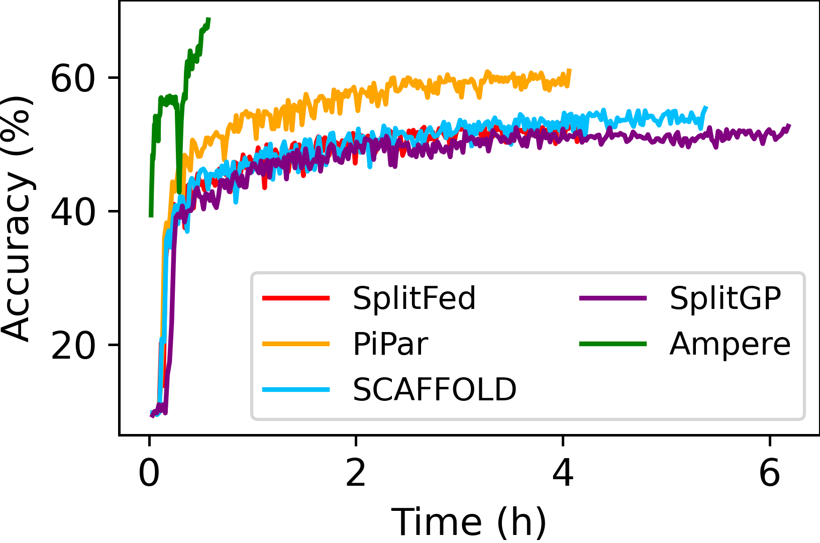
(a) MobileNet-L on CIFAR-10

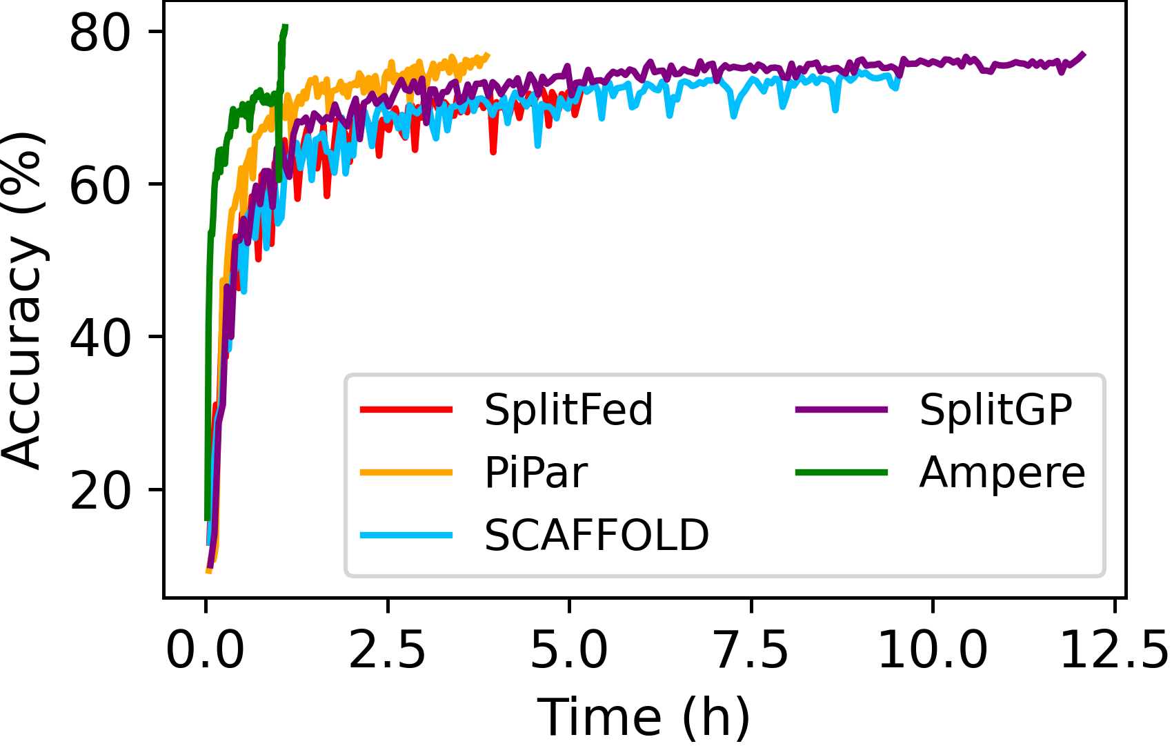
(b) VGG-11 on CIFAR-10

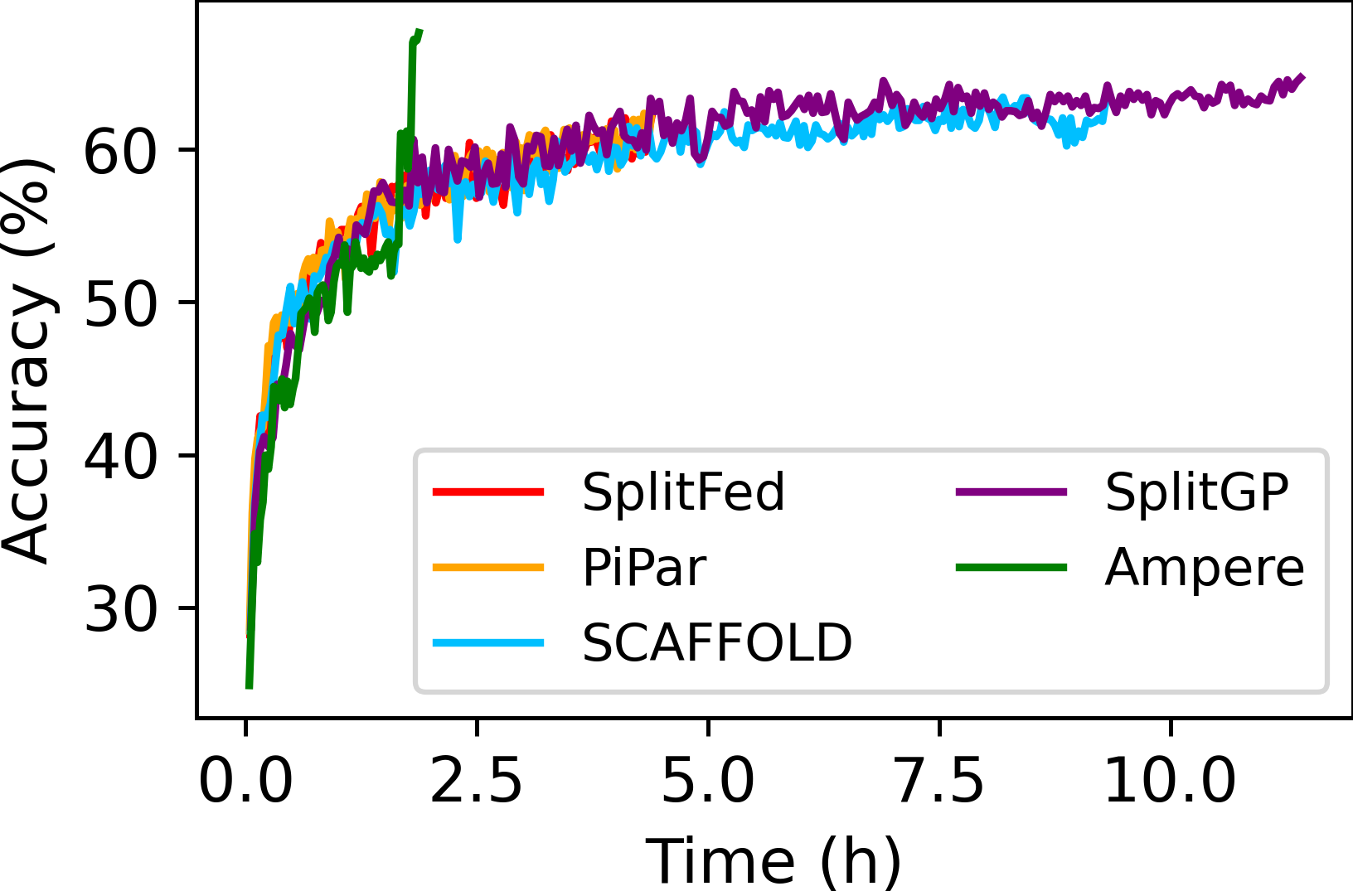
(c) Swin-T on CIFAR-10

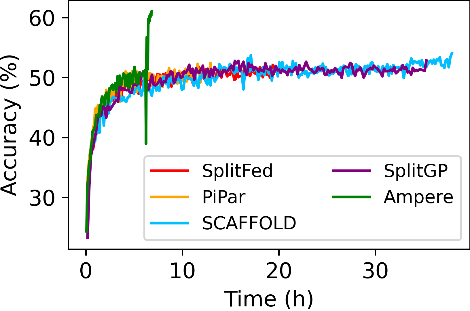
(d) ViT-S on CIFAR-10

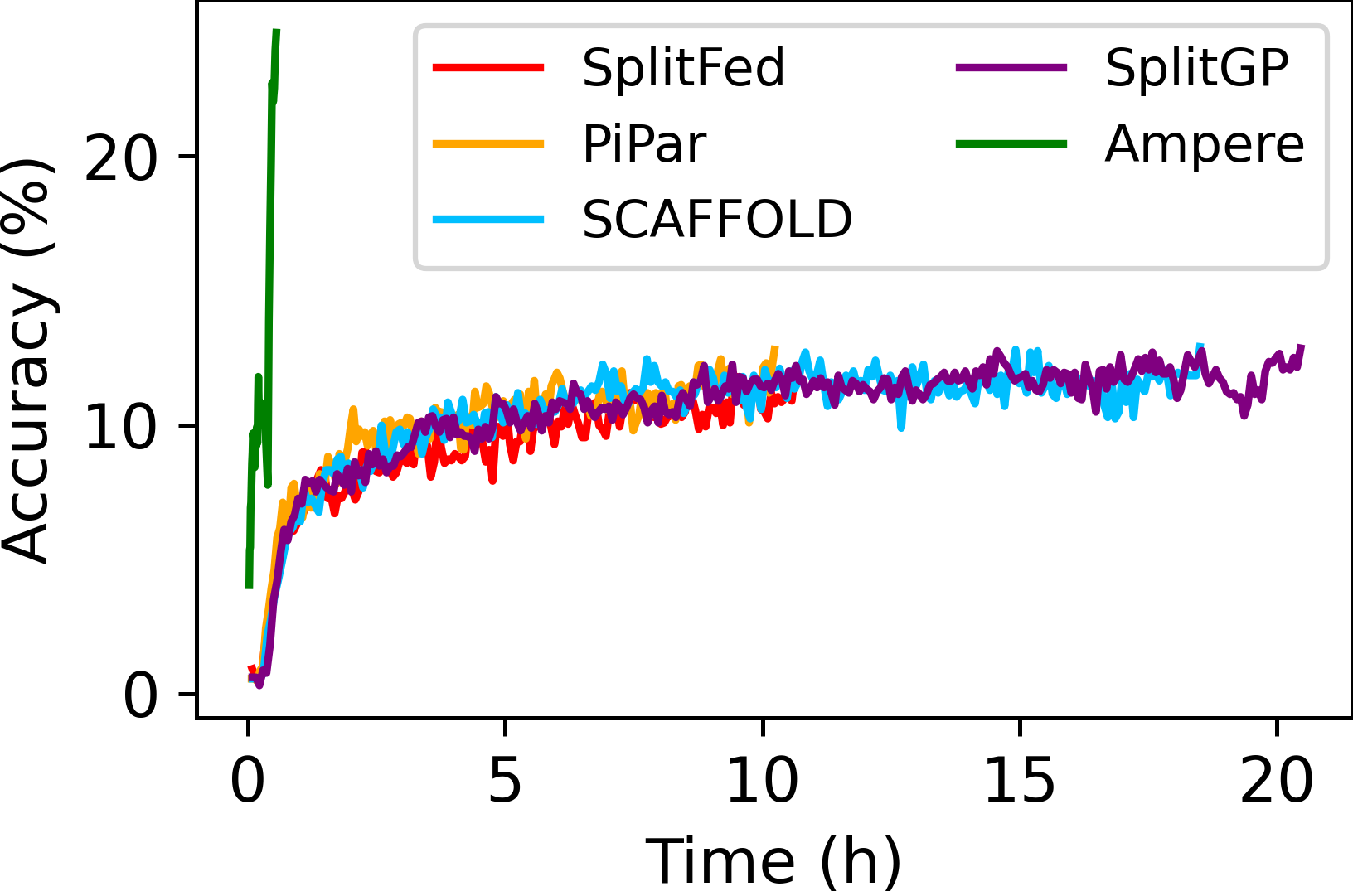
(e) MobileNet-L on Tiny ImageNet

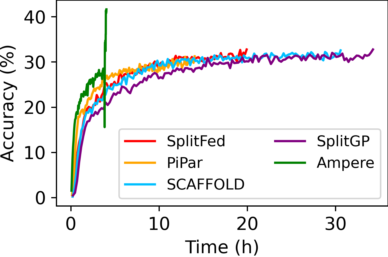
(f) VGG-11 on Tiny ImageNet

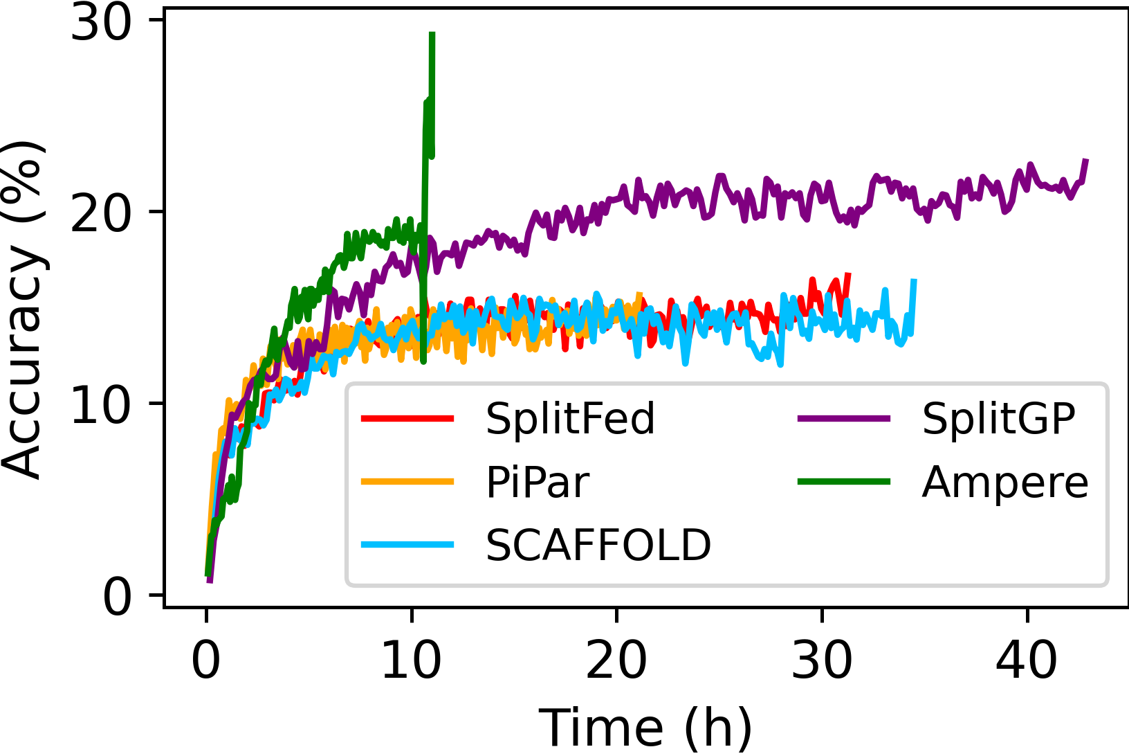
(g) Swin-T on Tiny ImageNet

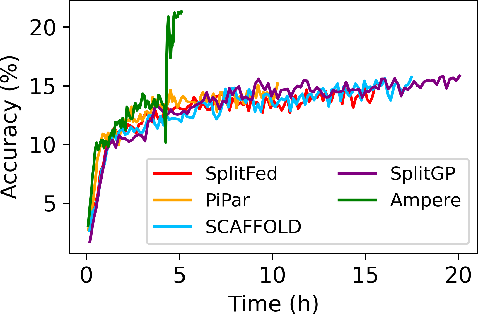
(h) ViT-S on Tiny ImageNet

Figure 8: Model accuracy (higher is better) versus training time (lower is better) for four models on two datasets.

5.2 Results

Ampere is evaluated against the four SFL-based baselines, focusing on model accuracy, communication and computation efficiency, and robustness against non-IID data. The experiments demonstrate that Ampere achieves higher model accuracy in a lower training time, significantly reduces device-server communication, and effectively mitigates the impact of data heterogeneity. Additionally, an ablation study demonstrates the benefits of activation consolidation in improving model accuracy.

TABLE IV: Total number of epochs for training (lower is better) four models on two datasets to convergence, using Ampere and three SFL baselines. For SFL baselines, both device and server blocks are trained in each epoch, whereas in Ampere  they are trained sequentially and, thus, noted separately as device epochs and server epochs.

		MobileNet-L		VGG-11		Swin-T		ViT-S
Baselines		CIFAR-10	Tiny ImageNet	CIFAR-10	Tiny ImageNet	CIFAR-10	Tiny ImageNet	CIFAR-10	Tiny ImageNet
SplitFed		200	159	115	109	120	218	131	105
PiPar		210	186	121	117	152	229	135	107
SCAFFOLD		240	258	184	156	216	223	244	110
SplitGP		300	298	211	148	240	240	201	115
	device	55	36	61	78	55	127	81	54
Ampere	server	32	10	25	24	22	21	46	88

5.2.1 Model Accuracy

We evaluate the model accuracy of Ampere against the SFL-based baselines to highlight its ability to achieve higher accuracy with a lower training time. Four models are trained on two datasets to converge. We apply early stopping [40] during training. Early stopping is guided by convergence - specifically when there is no improvement in validation accuracy for 15 consecutive epochs.

Figure 8 shows model accuracy against training time. In Ampere, model accuracy increases as the device block is first trained. Once the device block converges, server block training begins from scratch, causing a temporary accuracy drop in all cases shown in the figure. However, accuracy quickly recovers and surpasses the highest accuracy achieved during device block training. This confirms that final accuracy is improved from server-side training beyond what the auxiliary network alone can achieve.

Compared to SFL baselines that train server and device blocks together, Ampere achieves faster convergence for the device block and higher final accuracy at the end of server block training. Ampere achieves the highest final accuracy within the shortest training time than all baselines in all settings. Specifically, Ampere reduces total training time by 42.1% to 94.6% compared to the fastest baseline, while improving final accuracy by 2.95% to 13.26% on CIFAR-10 and 5.39% to 11.7% on Tiny ImageNet, compared to the baseline with the highest accuracy.

Table IV presents the number of training epochs required for each model to converge; the epochs for device and server training of Ampere are shown separately. Since the device block and auxiliary network are smaller than the entire model, they require fewer epochs to converge than SFL. Unlike SFL baselines, where devices must remain active throughout training, Ampere reduces device participation time between 44.3% to 96.3%, allowing devices to exit training earlier. This enables resource-constrained devices in real-world FL deployments, such as smartphones or IoT devices, to complete their training sooner and be available for other tasks without compromising model accuracy.

5.2.2 Communication and Computation

TABLE V: Device-server communication volume (GB) per device (lower is better) for training multiple models on two datasets to convergence, using FL (the communication volume is estimated), three SFL baselines, and Ampere.

	MobileNet-L		VGG-11		Swin-T		ViT-S
Baselines	CIFAR-10	Tiny ImageNet	CIFAR-10	Tiny ImageNet	CIFAR-10	Tiny ImageNet	CIFAR-10	Tiny ImageNet
FL (estimated)	12.72	10.05	48.3	42.42	48.55	88.94	38.25	30.66
SplitFed	61.03	193.85	70.20	265.80	55.00	398.82	245.06	196.47
PiPar	64.17	226.85	73.91	285.36	69.74	419.04	252.60	200.25
SCAFFOLD	73.23	314.55	112.42	380.50	99.19	408.16	459.76	207.36
SplitGP	91.63	370.60	128.92	368.13	110.0	439.10	376.01	215.24
Ampere	0.80	7.43	2.41	18.97	2.11	11.59	24.30	23.01

Figure 9: Total on-device computation (in TFLOPS; lower is better) for four different models on two datasets.

Here we demonstrate that Ampere reduces device-server communication volume while reducing on-device computation. Table V presents the total volume of data exchanged between each device and the server. By transferring activations only once, Ampere reduces communication volume by 88.3% to 99.1% compared to all SFL baselines.

Although FL is infeasible for these models on the devices due to memory constraints, we estimate its communication volume. Since the only difference between FL and SplitFed is where the computation is carried out, both require a similar number of training epochs. In each epoch, FL transfers two full models for aggregation (one upload and one download per device). We estimate the total communication volume of FL by multiplying the size of the two models by the number of training epochs. The results show that Ampere has lower communication than FL by 25.0% to 95.0%.

Additionally, Ampere requires fewer on-device training epochs than SFL baselines, reducing on-device computation, as measured in tera floating point operations (TFLOPS) in Figure 9. It achieves model convergence using only 6.87% to 96.2% of the on-device computation required by baselines.

5.2.3 Impact of Data Heterogeneity

Figure 10: Model accuracy (higher is better) for four models on two datasets for varying non-IID degree $\alpha$.

The impact of data heterogeneity in Ampere is captured by considering model accuracy and its standard deviation for different degrees of non-IID data relative to SFL baselines. $\alpha$ determines the degree of non-IID data, but its effect is not linear. We consider three representative non-IID degrees: IID ($\alpha=1$), moderately non-IID ($\alpha=0.33$), and severely non-IID ($\alpha=0.1$).

Figure 10 shows the model accuracy for different non-IID degrees. Ampere consistently outperforms all baselines across various models and datasets, achieving up to 24.35% higher accuracy. We measure the standard deviation in model accuracy to further quantify the impact of data heterogeneity. Ampere has a maximum standard deviation of 2.68 across all models and datasets, compared to 8.19, 5.75, 10.11, and 11.15 for SplitFed, PiPar, SCAFFOLD, and SplitGP, respectively. Ampere reduces the standard deviation of accuracy by 53.39% compared to the most stable baseline, indicating that Ampere is less impacted by non-IID data.

5.2.4 Impact of Activation Consolidation

To validate the effectiveness of activation consolidation, an ablation study that compares the model accuracy of Ampere with and without activation consolidation is considered.

In Ampere without activation consolidation, device block training remains unchanged. However, once the device block converges, each device sends its activations to the server, which maintains $K$ separate activation sets $\mathcal{A}_{k},k\in[K]$, each corresponding to a specific device as in an SFL system. After collecting all activations, the server trains $K$ individual server blocks on their respective activation sets and periodically aggregates them into a global server block, following the approach used in SFL baselines.

As shown in Figure 11, activation consolidation improves the model accuracy of Ampere between 6.04% to 13.2% across various models and datasets. Therefore, activation consolidation mitigates non-IID challenges and improves model accuracy in Ampere.

Figure 11: Model accuracy (higher is better) of Ampere with (w/) and without (w/o) Activation Consolidation on four different models and two datasets.

6 Related Work

In this section, we review existing methods that reduce communication costs and improve model accuracy in SFL, analyze their limitations, and contrast them with Ampere.

Reducing communication overhead arising from intermediate results. Existing research has explored four strategies to reduce communication overheads from exchange of activations and gradients in SFL systems:

(1) Generating gradients locally: Gradients are computed on devices to eliminate server-side gradient transmission, reducing SFL communication by half [41]. FedGKT [13] deploys local loss functions on devices and distills knowledge between the local and global models. EcoFed [10] reduces communication using a pre-trained device block but relies on public datasets. This limits its use in real-world FL scenarios as public data may not correspond to private device data. However, activations still need to be transferred, making communication in SFL systems higher than the FL counterparts.

(2) Overlapping communication and computation: PiPar [11] utilizes pipeline parallelism to overlap computation with activation transfers, thereby reducing idle time. This improves training efficiency by computing and communicating concurrently, but does not reduce the total communication volume or frequency.

(3) Clustering devices: FedAdapt [20] and ParallelSFL [42] group devices with similar compute and bandwidth capacities, optimizing communication within clusters. However, the trade-off between on-device computation and device-server communication is unresolved for individual devices.

(4) Compressing activation/gradients: In split learning, activations and gradients are compressed into lower-dimensional representations [6, 7]. However, these methods are not designed for FL with multiple devices and will reduce model accuracy. BaF [8] selectively compresses activations and applies a predictive reconstruction method, while randomized top-k sparsification [9] aims to retain accuracy. While these methods reduce activation size, they remain less efficient than FL which avoids activation transfers entirely.

Other FL systems reduce communication by training sub-models instead of full models on devices [43, 44] or using hyperdimensional computing [45]. However, these require high on-device computation and are not suited for SFL.

Existing methods fail to reduce the communication volume or frequency in SFL systems to FL levels because they still rely on iterative activation transfers. In contrast, Ampere reduces per-iteration activation transfers to a one-shot activation exchange, thereby significantly reducing both communication volume and frequency.

Improving model accuracy under non-IID data. Existing systems for improving FL model accuracy that train with non-IID data either modify local loss functions or global aggregation algorithms. FedAvgM [14] adjusts the way models are updated to make convergence more stable, reducing the impact of variable local updates. FedProx [15] introduces a regularization term that restricts local model updates, preventing them from deviating significantly from the global model. SCAFFOLD [16] addresses variations in local model updates by maintaining correction terms that adjust for differences in gradient updates across devices, ensuring that all devices contribute more uniformly to the global model. SplitGP[12] combines the gradients produced by local loss on devices and by global loss on the server to balance generalization and personalization, mitigating the non-IID issue.

While these systems mitigate the non-IID issue of the original data to some extent, they do not specifically address activation heterogeneity in SFL. Instead, each device block is trained separately on local data, and the server block continues to receive activations that reflect non-IID distributions. Thus, the server block learns inconsistent feature representations from device-specific activations, reducing generalization and degrading model accuracy.

Ampere addresses the challenge by consolidating activations into a single dataset for server block training. As the consolidated dataset is more homogeneous than each device’s activations, Ampere improves overall model accuracy without requiring specialized aggregation algorithms.

7 Conclusion and Discussion

Three challenges limit the use of a Split Federated Learning (SFL) system in the real-world. Firstly, it has high communication overheads arising from frequent exchanges of intermediate activations and gradients between devices and the server. Secondly, the trade-off between on-device computation and device-server communication when selecting the split point leads to less optimal performance. Thirdly, data heterogeneity impacts model accuracy.

We propose Ampere  a new collaborative training system that goes beyond SFL to address these challenges by introducing three key innovations: (1) unidirectional inter-block training, a novel technique to sequentially trains device and server layers instead of using end-to-end backpropagation in SFL systems. This eliminates the computation and communication trade-off and achieves both optimal on-device computation and device-server communication at the same split point; (2) a lightweight auxiliary network generation method, which decouples device and server training, eliminating iterative transfers of intermediate results in SFL systems and significantly reducing communication volume and frequency; and (3) an activation consolidation method, which trains a single server block on a unified activation set generated by all devices using converged device layers, rather than training on device-specific, non-IID activations as in SFL, thereby mitigating the impact of data heterogeneity.

Ampere is evaluated against state-of-the-art SFL baselines using CNN and transformer-based models. Results show that Ampere improves accuracy by up to 13.26% while reducing training time by up to 94.6% and reduces device-server communication overhead by up to 99.1% and on-device computation by up to 93.13%. Furthermore, Ampere reduces the standard deviation of accuracy by 53.39% for various non-IID degrees compared to other baselines, indicating that it is less impacted by non-IID data.

While Ampere effectively addresses key challenges in split federated learning, there are open avenues for improvement as considered below.

Privacy considerations. Like most SFL systems, Ampere requires devices to upload intermediate activations to the server. Although activations are transferred only once in Ampere, prior research [46] has shown that such intermediate features may still be vulnerable to inversion attacks, particularly in vision models. Ampere is compatible with several existing privacy-preserving techniques, including differentially private training (e.g., DP-SGD [47]), homomorphic encryption [48] for encrypted activation transfer, and certified defences such as PixelDP [49] that target privacy leakage from intermediate representations. These defences can be integrated and evaluated in the context of one-shot activation transfer to extend Ampere for privacy-sensitive applications.

Hardware constraints. Although Ampere significantly reduces on-device computation compared to existing FL and SFL systems, it still assumes the availability of devices capable of executing a shallow device block and a lightweight auxiliary network. Severely resource-constrained platforms, such as microcontrollers or bare-metal sensors, are outside the current scope of this work. Extending the system to support such ultra-low-end devices remains a direction for future investigation.

Zihan Zhang is a PhD student at University of St Andrews. He was previously a researcher at Noah’s Ark Lab, Huawei. Prior to that, he obtained a Master’s degree in Data Science with distinction from University of Edinburgh and a Bachelor degree in Mathematics from Shandong University. His interests include collaborative machine learning and cloud/edge computing.

Leon Wong is the Research Collaboration and Engineering Lead for Autonomous Networks Research & Innovation in Rakuten Mobile, Inc. He is currently serving as chairman of ITU-T Focus Group of Autonomous Networks (FG-AN), established under ITU-T Study Group 13 - Future networks and emerging network technologies. He is also the co-chair of FG-AN Ad hoc group for Japan’s Telecommunication Technology Committee (TTC).

Blesson Varghese received the PhD degree in computer science from the University of Reading, UK on international scholarships. He is a Reader in computer science at the University of St Andrews, UK, and the Principal Investigator of the Edge Computing Hub. He was a previous Royal Society Short Industry Fellow. His interests include distributed systems that span the cloud-edge-device continuum and edge intelligence applications. More information is available from www.blessonv.com.

References

- [1] H. B. McMahan, E. Moore, D. Ramage, S. Hampson, and B. A. y Arcas, “Communication-Efficient Learning of Deep Networks from Decentralized Data,” in International Conference on Artificial Intelligence and Statistics, 2016. [Online]. Available: https://api.semanticscholar.org/CorpusID:14955348
- [2] J. Konečný, B. McMahan, and D. Ramage, “Federated Optimization: Distributed Optimization Beyond the Datacenter,” CoRR, 2015.
- [3] J. Konečný, H. B. McMahan, D. Ramage, and P. Richtárik, “Federated Optimization: Distributed Machine Learning for On-Device Intelligence,” CoRR, vol. abs/1610.02527, 2016.
- [4] J. Konečný, H. B. McMahan, F. X. Yu, P. Richtarik, A. T. Suresh, and D. Bacon, “Federated Learning: Strategies for Improving Communication Efficiency,” in NIPS Workshop on Private Multi-Party Machine Learning, 2016. [Online]. Available: https://arxiv.org/abs/1610.05492
- [5] C. Thapa, M. A. P. Chamikara, and S. Camtepe, “SplitFed: When Federated Learning Meets Split Learning,” AAAI Conference on Artificial Intelligence, vol. 36(8), pp. 8485–8493, 2022.
- [6] J. Shao and J. Zhang, “BottleNet++: An End-to-End Approach for Feature Compression in Device-Edge Co-Inference Systems,” in 2020 IEEE International Conference on Communications Workshops, 2020, pp. 1–6.
- [7] C.-Y. Hsieh, Y.-C. Chuang, and A.-Y. Wu, “C3-SL: Circular Convolution-Based Batch-Wise Compression for Communication-Efficient Split Learning,” in IEEE 32nd International Workshop on Machine Learning for Signal Processing, 2022, pp. 1–6.
- [8] H. Choi, R. A. Cohen, and I. V. Bajić, “Back-And-Forth Prediction for Deep Tensor Compression,” in IEEE International Conference on Acoustics, Speech and Signal Processing, 2020, pp. 4467–4471.
- [9] F. Zheng, C. Chen, L. Lyu, and B. Yao, “Reducing Communication for Split Learning by Randomized Top-k Sparsification,” in Proceedings of the Thirty-Second International Joint Conference on Artificial Intelligence, 2023.
- [10] D. Wu, R. Ullah, P. Rodgers, P. Kilpatrick, I. Spence, and B. Varghese, “ EcoFed: Efficient Communication for DNN Partitioning-Based Federated Learning ,” IEEE Transactions on Parallel & Distributed Systems, vol. 35, no. 03, pp. 377–390, 2024.
- [11] Z. Zhang, P. Rodgers, P. Kilpatrick, I. Spence, and B. Varghese, “PiPar: Pipeline Parallelism for Collaborative Machine Learning,” Journal of Parallel and Distributed Computing, vol. 193, p. 104947, 2024.
- [12] D.-J. Han, D.-Y. Kim, M. Choi, C. G. Brinton, and J. Moon, “SplitGP: Achieving Both Generalization and Personalization in Federated Learning,” in IEEE Conference on Computer Communications, 2023, pp. 1–10.
- [13] C. He, M. Annavaram, and S. Avestimehr, “Group Knowledge Transfer: Federated Learning of Large CNNs at the Edge,” in Proceedings of the 34th International Conference on Neural Information Processing Systems, 2020.
- [14] T. H. Hsu, H. Qi, and M. Brown, “Measuring the Effects of Non-Identical Data Distribution for Federated Visual Classification,” CoRR, vol. abs/1909.06335, 2019.
- [15] T. Li, A. K. Sahu, M. Zaheer, M. Sanjabi, A. Talwalkar, and V. Smith, “Federated Optimization in Heterogeneous Networks,” in Proceedings of the Third Conference on Machine Learning and Systems, 2020.
- [16] S. P. Karimireddy, S. Kale, M. Mohri, S. Reddi, S. Stich, and A. T. Suresh, “SCAFFOLD: Stochastic Controlled Averaging for Federated Learning,” in Proceedings of the 37th International Conference on Machine Learning, H. D. III and A. Singh, Eds., vol. 119, 13–18 Jul 2020, pp. 5132–5143.
- [17] A. Howard, M. Sandler, G. Chu, L. Chen, B. Chen, M. Tan, W. Wang, Y. Zhu, R. Pang, V. Vasudevan, Q. V. Le, and H. Adam, “Searching for MobileNetV3,” IEEE/CVF International Conference on Computer Vision, pp. 1314–1324, 2019.
- [18] A. Krizhevsky, V. Nair, and G. Hinton, “CIFAR-10 (Canadian Institute for Advanced Research),” 2009, available at https://www.cs.toronto.edu/~kriz/cifar.html.
- [19] A. Krizhevsky and G. Hinton, “Learning Multiple Layers of Features from Tiny Images,” Master’s thesis, Department of Computer Science, University of Toronto, 2009.
- [20] D. Wu, R. Ullah, P. Harvey, P. Kilpatrick, I. Spence, and B. Varghese, “FedAdapt: Adaptive Offloading for IoT Devices in Federated Learning,” IEEE Internet of Things Journal, vol. 9, no. 21, pp. 20 889–20 901, 2022.
- [21] M. Zeiler and R. Fergus, “Visualizing and Understanding Convolutional Networks,” in European Conference on Computer Vision, 2014, pp. 818–833.
- [22] J. Yosinski, J. Clune, Y. Bengio, and L. Hod, “How Transferable Are Features in Deep Neural Networks?” in Proceedings of the 28th International Conference on Neural Information Processing Systems, vol. 2, 2014, pp. 3320–3328.
- [23] Y. LeCun, Y. Bengio, and G. Hinton, “Deep Learning,” Nature, vol. 521, no. 7553, pp. 436–444, 2015. [Online]. Available: https://doi.org/10.1038/nature14539
- [24] X. Li, K. Huang, W. Yang, S. Wang, and Z. Zhang, “On the Convergence of FedAvg on Non-IID Data,” in International Conference on Learning Representations, 2020. [Online]. Available: https://openreview.net/forum?id=HJxNAnVtDS
- [25] E. Belilovsky, M. Eickenberg, and E. Oyallon, “Decoupled Greedy Learning of CNNs,” in Proceedings of the 37th International Conference on Machine Learning, 2020.
- [26] L. Bottou, F. E. Curtis, and J. Nocedal, “Optimization Methods for Large-Scale Machine Learning,” SIAM Review, vol. 60, no. 2, pp. 223–311, 2018.
- [27] Z. Huo, B. Gu, and H. Huang, “Training Neural Networks Using Features Replay,” in Advances in Neural Information Processing Systems, vol. 31. Curran Associates, Inc., 2018.
- [28] Y. Zhang, J. C. Duchi, and M. J. Wainwright, “Communication-Efficient Algorithms for Statistical Optimization,” The Journal of Machine Learning Research, vol. 14, no. 1, p. 3321–3363, 2013.
- [29] S. U. Stich, “Local SGD Converges Fast and Communicates Little,” in International Conference on Learning Representations, 2019.
- [30] S. U. Stich, J.-B. Cordonnier, and M. Jaggi, “Sparsified SGD with memory,” in Proceedings of the 32nd International Conference on Neural Information Processing Systems, 2018, p. 4452–4463.
- [31] H. Yu, S. Yang, and S. Zhu, “Parallel Restarted SGD with Faster Convergence and Less Communication: Demystifying Why Model Averaging Works for Deep Learning,” in Proceedings of the Thirty-Third AAAI Conference on Artificial Intelligence, 2019.
- [32] H. E. Robbins, “A Stochastic Approximation Method,” Annals of Mathematical Statistics, vol. 22, pp. 400–407, 1951.
- [33] S. Maheshwari, D. Raychaudhuri, I. Seskar, and F. Bronzino, “Scalability and Performance Evaluation of Edge Cloud Systems for Latency Constrained Applications,” in 2018 IEEE/ACM Symposium on Edge Computing, 2018, pp. 286–299.
- [34] K. Simonyan and A. Zisserman, “Very Deep Convolutional Networks for Large-scale Image Recognition,” 3rd International Conference on Learning Representations, p. 1–14, 2015.
- [35] Z. Liu, Y. Lin, Y. Cao, H. Hu, Y. Wei, Z. Zhang, S. Lin, and B. Guo, “Swin Transformer: Hierarchical Vision Transformer using Shifted Windows,” in Proceedings of the IEEE/CVF International Conference on Computer Vision, 2021, pp. 9992–10 002.
- [36] A. P. Steiner, A. Kolesnikov, X. Zhai, R. Wightman, J. Uszkoreit, and L. Beyer, “How to Train Your ViT? Data, Augmentation, and Regularization in Vision Transformers,” Transactions on Machine Learning Research, 2022. [Online]. Available: https://openreview.net/forum?id=4nPswr1KcP
- [37] A. Dosovitskiy, L. Beyer, A. Kolesnikov, D. Weissenborn, X. Zhai, T. Unterthiner, M. Dehghani, M. Minderer, G. Heigold, S. Gelly, J. Uszkoreit, and N. Houlsby, “An Image is Worth 16x16 Words: Transformers for Image Recognition at Scale,” in International Conference on Learning Representations, 2021.
- [38] O. Russakovsky, J. Deng, H. Su, J. Krause, S. Satheesh, S. Ma, Z. Huang, A. Karpathy, A. Khosla, M. Bernstein, A. C. Berg, and L. Fei-Fei, “ImageNet Large Scale Visual Recognition Challenge,” International Journal of Computer Vision, vol. 115, no. 3, pp. 211–252, 2015.
- [39] D. A. E. Acar, Y. Zhao, R. Matas, M. Mattina, P. Whatmough, and V. Saligrama, “Federated Learning Based on Dynamic Regularization,” in International Conference on Learning Representations, 2021.
- [40] L. Prechelt, “Early Stopping—But When?” Neural Networks: Tricks of the Trade, vol. 7700, pp. 53–67, 2012.
- [41] D.-J. Han, H. I. Bhatti, J. Lee, and J. Moon, “Accelerating Federated Learning with Split Learning on Locally Generated Losses,” in International Conference on Machine Learning Workshop on Federated Learning for User Privacy and Data Confidentiality, 2021.
- [42] Y. Liao, Y. Xu, H. Xu, Z. Yao, L. Huang, and C. Qiao, “ParallelSFL: A Novel Split Federated Learning Framework Tackling Heterogeneity Issues,” in Proceedings of the 30th Annual International Conference on Mobile Computing and Networking, 2024, p. 845–860.
- [43] A. Li, J. Sun, P. Li, Y. Pu, H. Li, and Y. Chen, “Hermes: An Efficient Federated Learning Framework for Heterogeneous Mobile Clients,” in Proceedings of the 27th Annual International Conference on Mobile Computing and Networking, 2021, p. 420–437.
- [44] C. Niu, F. Wu, S. Tang, L. Hua, R. Jia, C. Lv, Z. Wu, and G. Chen, “Billion-Scale Federated Learning on Mobile Clients: a Submodel Design with Tunable Privacy,” in Proceedings of the 26th Annual International Conference on Mobile Computing and Networking, 2020.
- [45] Q. Zhao, K. Lee, J. Liu, M. Huzaifa, X. Yu, and T. Rosing, “FedHD: Federated Learning with Hyperdimensional Computing,” in Proceedings of the 28th Annual International Conference on Mobile Computing And Networking, 2022, p. 791–793.
- [46] A. Mahendran and A. Vedaldi, “Understanding Deep Image Representations by Inverting Them,” in Proceedings of the IEEE conference on computer vision and pattern recognition, 2015, pp. 5188–5196.
- [47] M. Abadi, A. Chu, I. Goodfellow, H. B. McMahan, I. Mironov, K. Talwar, and L. Zhang, “Deep Learning with Differential Privacy,” in Proceedings of the 2016 ACM SIGSAC Conference on Computer and Communications Security, 2016, p. 308–318.
- [48] J. H. Cheon, A. Kim, M. Kim, and Y. Song, “Homomorphic Encryption for Arithmetic of Approximate Numbers,” Advances in Cryptology - ASIACRYPT, pp. 409–437, 2017.
- [49] M. Lecuyer, V. Atlidakis, R. Geambasu, D. Hsu, and S. Jana, “Certified Robustness to Adversarial Examples with Differential Privacy,” in 2019 IEEE Symposium on Security and Privacy (SP), 2019, pp. 656–672.