Amplitude Walk in Fast Timing: The Role of Dual Thresholds

Abstract

In preparation for HL-LHC operation, a number of new detector systems are being constructed with timing precision on physics objects of $\leq 50$ picoseconds. These time stamps will reduce the level of pileup induced backgrounds as the number of interactions per crossing will reach of order 100-200[1]. In this report we note that this high pileup level will necessitate a new approach to calibration of these large timing arrays (typically with several $\times 10^{5}$ channels) since a single t₀ reference is hard to come by in regular data taking. We demonstrate that enhancing the usual pair of timing ASIC data (ie threshold time and amplitude or time-over-threshold) with a 2nd threshold time greatly simplifies the analysis of amplitude walk. Since slope at threshold is directly relevant for amplitude walk, day-1 walk calibration can often have an analytical solution.

1 Introduction

A common aspect of time-of-flight systems is the need to correct the time recorded at fixed threshold. Amplitude fluctuations induce "walk" relative to the actual time of arrival . For this purpose, most systems record also the pulse amplitude or the time-over-threshold (proportional to the amplitude). As we will see below, this traditional measurement is really a poor relation of a "pulse slope at threshold" measurement, since the latter is what directly relates to the time walk.

Nevertheless large timing systems have been calibrated successfully in previous hadron collider experiments. In CDF timing was deployed in the electromagnetic calorimeter[2] and the necessary calibrations were performed using clean samples- ie Z${}^{0}\rightarrow e^{+}e^{-}$. Since, in CDF, pileup never exceeded "a few" and the total number of channels was less than $10^{5}$ the calibration was less demanding than expected for HL-LHC.

The ALICE experiment Time-of-Flight system[3] consists of $\sim 150$k channels based on MRPC’s and during run 1 they reported a time resolution of 82 picoseconds. During run 2, after a renewed effort to refine walk calibration, an improved resolution of 56 picoseconds was achieved. It should be noted that the ALICE experiment runs primarily under low pileup conditions so a t₀ reference was likely a practical tool for calibration.

Since it is a common goal to achieve the performance spec of the HL-LHC timing detectors as soon as possible, the ALICE case should be an incentive to explore calibration strategy well in advance. The new technologies employed in CMS and ATLAS promise as low as 30 picosecond Day-1 resolution so long as initial calibration is successful.

Also, these detectors are exposed to a challenging radiation environment at the HL-LHC requiring, in some cases, change of operating conditions several times per year- implying frequent re-calibration.

The most frequent calibration procedure when time-at-threshold and amplitude are recorded is to take a controlled data set where the time of arrival and, if necessary, tracking information are available and generate an "ad hoc" parametrization for the walk. It is unlikely that such controlled data will be readily available at day-1 in HL-LHC for these arrays of several $\times 10^{5}$ channels.

We will give examples of cases where adding to the usual timing data the "pulse slope at threshold" greatly simplifies the task of Day-1 walk calibration.

1.1 Outline

Motivated by simpler examples we demonstrate that, also for the ASIC under study, the amplitude walk calibration reduces to a simple linear expression relating inverse of the pulse slope at threshold to walk.

A single coefficient gives the relation between “corrected time" and the time and slope at threshold measured in a given channel. Of course, reducing initial calibration to a single, possibly channel dependent, constant is an advantage.

From the sample of channels investigated below, we find that the calibration constants do vary among channels($\pm 22\%$) but this variation can be taken into account from the initial stand-alone calibration run (where slope and charge are recorded).

The above plan to put in place “Day-1" walk calibration never uses an external time reference (t₀) . It assumes that the following study gives a complete prescription for initializing the constants of every channel.

In order to arrive at this prescription we, of course, employ a stable time reference in the laser setup to validate this prescription. But “Day-1" calibration is based only on data internal to the detector subsystem (BTL in the case of CMS).

2 Slope Measurement with dual thresholds

What is the alternative? One particular ASIC developed for the CMS Barrel Timing Layer[5] -the TOFHIR2C[6]- incorporates an additional timing discriminator whose threshold setting can be adjusted to slightly differ from the first discriminator as in. Fig. 1(left). The threshold settings are given by the corresponding DAC values which control them. If the second threshold is set just above the first -see Figure 1(left)- by $\delta$I (the TOFHIR2C uses current discriminators, so “thr" implies $I_{threshold}$ in this paper) then:

$$Slope=\frac{thr_{2}-thr_{1}}{dt}$$ (2.1)

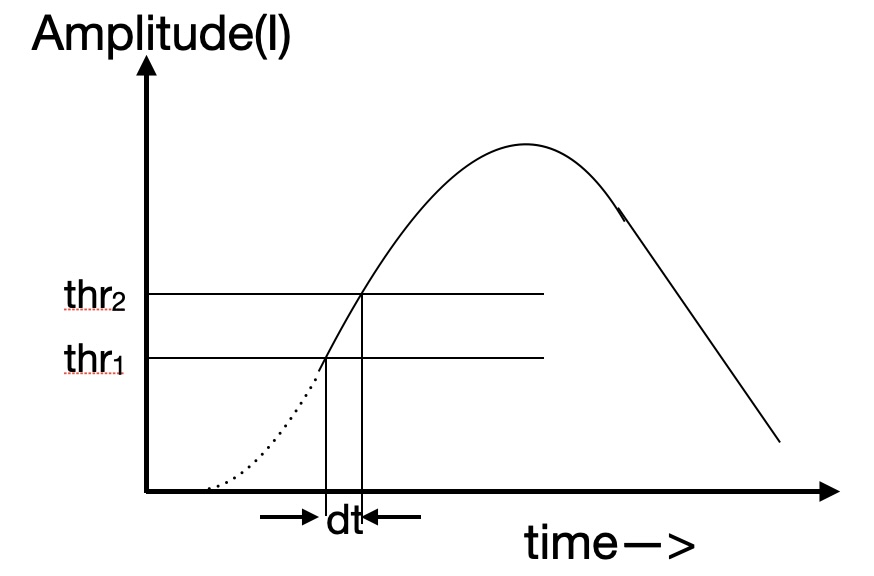
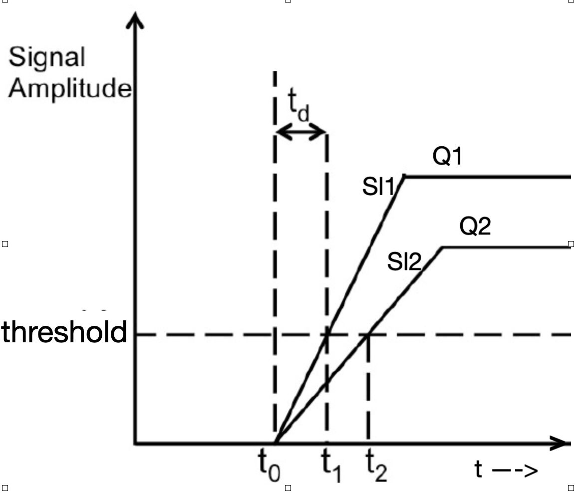
Figure 1: The use of dual thresholds to obtain “pulse slope at threshold" as used throughout this paper(left). A simple example(right) illustrating the direct relation between “pulse slope at threshold" and walk for two different signals with slopes S1 and S2 and amplitudes Q1 and Q2.

In an earlier note[7] we discussed the possible utility of this measurement for reducing time jitter due to dark count noise in SiPMs. This would require event-by-event measurement of the slope in order to detect disruption of the correlation between slope and amplitude arising from super-posed 1/f noise (characteristic of dark count noise)[8]. It turns out that the measurement of slope is often less precise than that of amplitude so it would take special care to exploit such event-by-event tools.

The procedure we propose for walk correction does not require event-by-event recording of the slope. The walk correction deals with the average behavior of a channel- in particular benefiting from the stability of the relation between amplitude and slope. One need only record data with sufficient statistics to capture the slope corresponding to a given value of amplitude from an ensemble of a few hundred slope measurements (typically with 10-20$\%$ fluctuation) and then create a mapping or look up table so that a measurement of amplitude ( within $\leq 3\%$ in our case[6]) determines the slope at threshold in a given event. In the following we discuss how this is used.

2.1 Naive case

We wish to correct to the same time of arrival irrespective of amplitude. We illustrate the relation between walk and pulse slope at threshold with the simple example in Figure 1(right). Consider two pulses given equal time of arrival but differing amplitudes (Q1,Q2). In this example the slopes (Sl1, Sl2) are clearly proportional to the corresponding amplitude (ie charge, Q). We will see later that, more generally, slope and Q are usually linearly related but with a possible offset.

The slopes (Figure 1, right) are given by:

$$Slope_{i}=\frac{I_{th}}{t_{i}-t_{0}}$$ (2.2)

so the general rule for correcting to a common time, independent of Q is:

$$t_{0}=t_{i}-\frac{I_{th}}{Slope_{i}}$$ (2.3)

Since, in the remainder of this paper we will discover that the correction for walk is generally a linear expression in inverse slope we will adopt the notation Amplitude Walk Coefficient (AWC- with the same dimensions as threshold) and re-write eqn. 2.3 as:

$$t_{corrected}=t_{i}-AWC*\frac{1.}{Slope_{i}}$$ (2.4)

2.1.1 Lessons from Naive Case

Our aim is to reduce the walk calibration to a simple analytic procedure that eliminates the need for controlled data sets which establish ad hoc remedies. The naive case illustrates the fact that amplitude walk is all about pulse slope and the calibration may reduce to the determination of a single parameter-the AWC. The common element in timing ASICs -ie recording pulse amplitude or time over threshold - should really be viewed as a proxy for slope. We will see that the dual threshold feature from which we can measure slope simplifies the calibration.

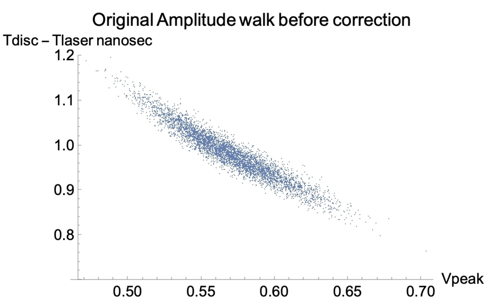
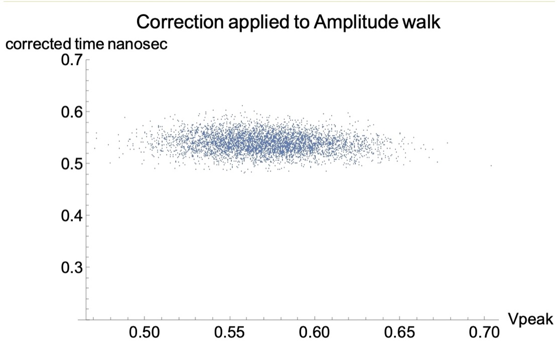
Figure 2: The resulting walk corrected data (right) after application of an analytic expression in pulse slope for a system with linear response- taken from ref. 7.

2.2 Departure from the Naive Case

The key criterion for applicability of the method we propose is linearity.

• In the simplest case- the naive example above (Figure 1, right)- the timing pulse leading edge is simply a straight line. In practical circuits, bandwidth limits the transition from baseline but this has a minor effect on this example. So in this case one needs only knowledge of the slope for a given event.

• More generally, linearity refers to the system response. If response is linear then waveforms of different amplitudes will be identical so long as they are re-scaled by amplitude. For this case, the benefit of recording the pulse slope was demonstrated in an earlier report[9] and the effectiveness is illustrated in Figure 2, which is taken from that report. So again, for this case one only needs knowledge of the slope for a given event.

• Lastly, and for the remainder of this paper, we deal with a case where neither notion of linearity applies- the TOFHIR2C[6] ASIC. We will see that, in this case, pulse slope and amplitude information complement one another, yielding once again a single parameter correction- the AWC.

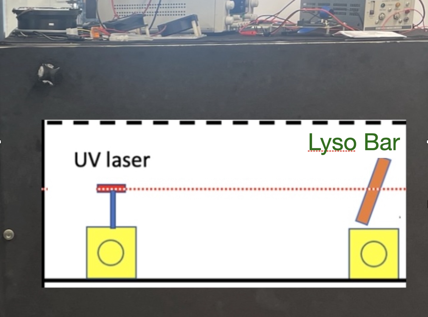
Figure 3: The lab setup used for these data. A pulsed UV laser sequentially excites scintillation response in a LYSO array.

3 Data Sets Used for this Paper

The laboratory data on which the following analysis is based were recorded using a test stand at the PETSYS company which produced the TOFHIR2C ASIC under contract with CMS. The basic setup, shown in Figure 3, consists of a fast pulsed UV laser that sequentially illuminates an array of 16 LYSO bars. The LYSO array is a prototype for the CMS BTL MIP timing detector(MTD) upgrade described in ref.[10]. Each 54.7$\times 3.0\times 3.75mm^{3}$ bar has Hamamatsu SiPMs coupled to both ends which are read by a single 32-channel TOFHIR2C ASIC. Each LYSO bar is wrapped in reflective tape to prevent optical crosstalk except for a small opening that allows light from a 375 nm pulsed laser to directly excite the LYSO bar.

Further details of the LYSO/SiPM properties can be found in ref.[10] but, for the purposes of this paper, it is sufficient to keep in mind that the detector is intrinsically linear in response so the departure from overall linearity of the system is attributed to the ASIC itself.

The TOFHIR2C employs effectively single delay line shaping using R-C networks internal to the chip and many aspects of its performance are captured in the CADENCE tool which was used in the design. However, in our experience with the CADENCE tool, it hasn’t been possible to reproduce the non-linear aspects which complicate the following analysis.

In this respect, we develop a data driven solution within which several features can be justified from simple considerations.

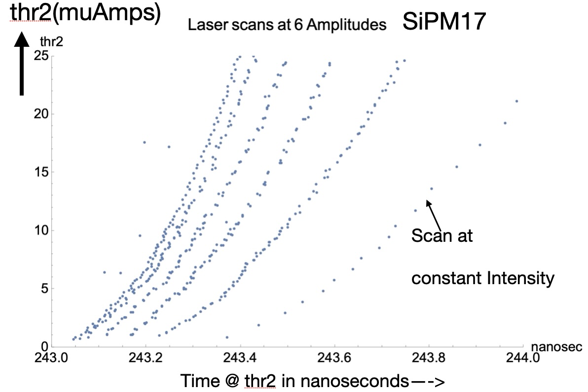
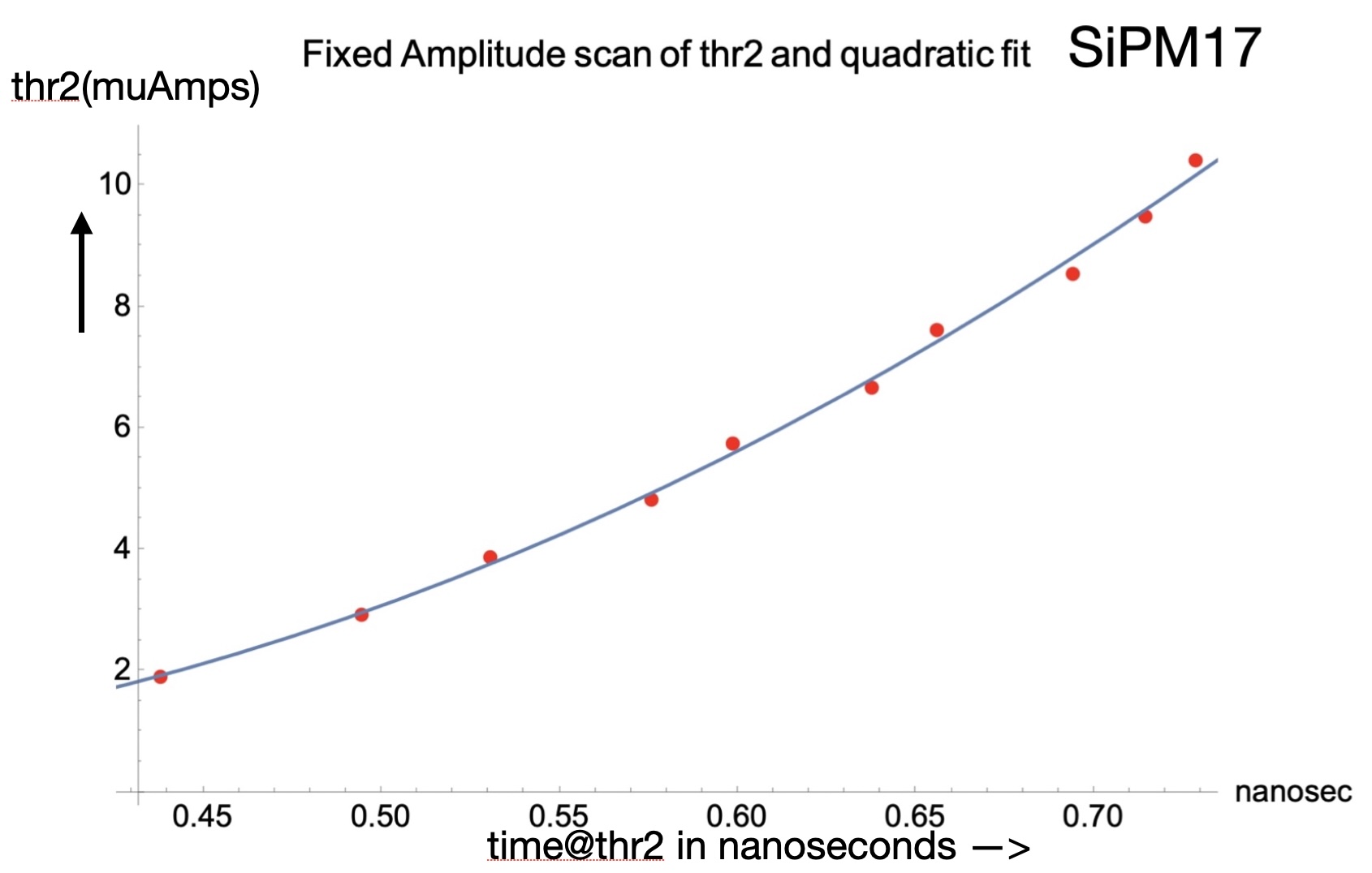
Figure 4: A typical data set for one channel (SiPM17) , where each point is an average of $\sim 200$ laser shots(left) and the resulting curves represent the pulse shape at the input of the timing discriminator for each laser intensity. Since we present results for a range of thresholds, we capture times (ie walk relative to t_corrected) and slopes in a quadratic fit (right) for this analysis.

3.1 Laser Data

In a particular dataset we step through all 16 bars, one at a time. For each bar we step through a sequence of 6 laser intensity settings which cover the SiPM output range that matches the TOFHIR2C ADC limits when the SiPM bias is matched to the expected conditions at the start of operations-ie “day-1 conditions".

Finally, the laser pulses are repeated several hundred times at each setting of the TOFHIR2C timing threshold (we are scanning timing discriminator 2- hence the labels “thr2"), which spans from roughly the baseline to several tens of $\mu$Amps. The threshold setting is controlled by a DAC with 0.3125 $\mu$Amp least count and the baseline is measured separately for each channel.

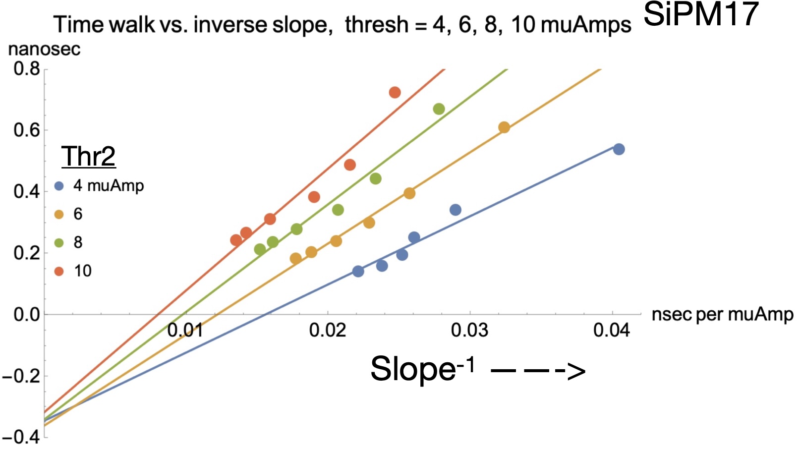
Figure 5: The time at threshold(ie $t_{i}$ in eqn 2.4) vs. inverse slope are well fitted to a linear relation in this and all other channels. Measurements are repeated for 4 different “thr2" settings.

Following this procedure we obtain the data plotted in Figure 4(left) for a given channel. There are 6 laser intensities in this figure and for each intensity the points accumulated from $\sim 200$ laser pulses at each threshold setting map out the leading edge in the neighborhood of the expected useful threshold (typically 4-6 $\mu$Amp).

Referring to the 6 leading edge profiles in Figure 4(left), it is easily verified that the system does not obey the linearity (ie scaling) behavior defined above.

We can use the scans in Figure 4 to capture the pulse slope (the time derivative of the quadratic fits) and timestamp (ie $t_{i}$ of eqn 2.4) at threshold for the 6 pulse amplitudes. For the remaining discussion we take the measured points for each channel and perform quadratic fits (see Figure 4-right) in order to capture time and slope in a range of threshold settings. Also, in Figure 4-right, we remove the arbitrary $\sim 242$ nanosecond offset of the laser time stamp.

For each channel we map out the relation between inverse slope and time at threshold at 6 different intensity settings. The results for a typical channel are displayed in Figure 5. In all cases the data are well described by a linear dependence of time at threshold ( $t_{i}$) on the inverse slope and we conclude that the TOFHIR2C data for a given threshold follow the simple form of eqn. 2.4. The slope of the fitted lines correspond to the coefficient “AWC" we defined above.

Unlike the linear examples discussed above, we have no a priori expectation for the value of the Amplitude Walk Correction. So we next ask the question “what is the spread in AWC values" for our sample of 25 channels. More importantly, since we are looking for a procedure to calibrate a much larger sample, “can we anticipate individual AWC values using TOFHIR2C-only calibration data". The answer appears to be “yes".

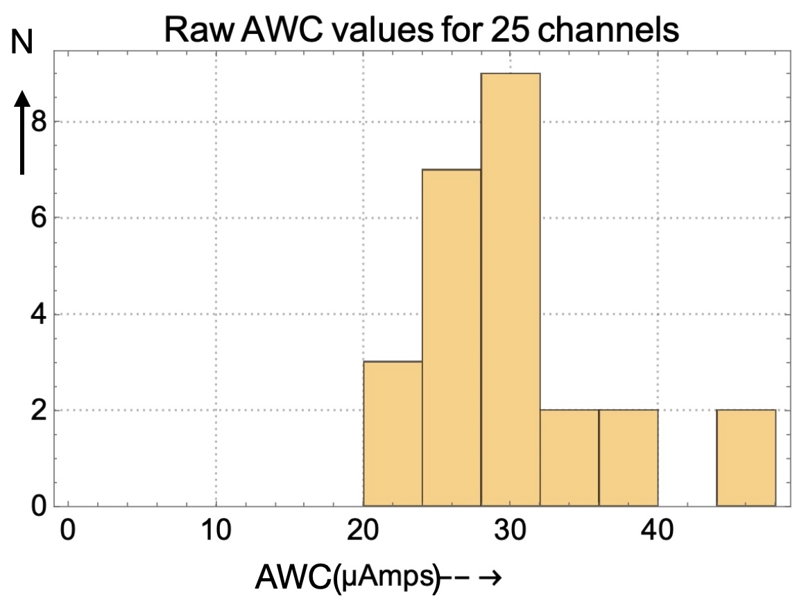
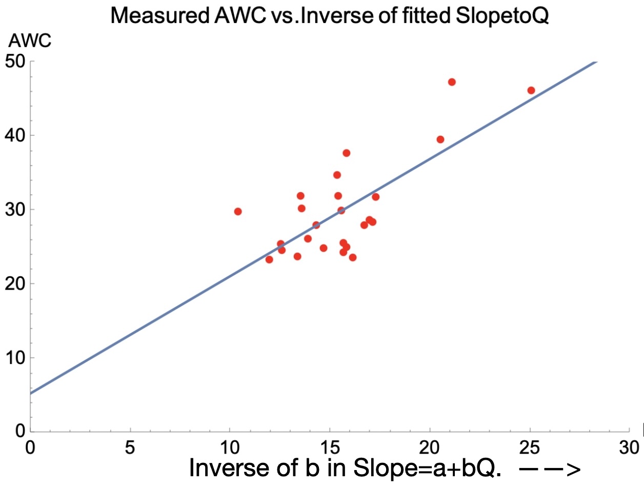
Figure 6: The slopes (left) fitted, as in Figure 5, at 6 $\mu$Amp threshold have an rms spread of $\sim 22\%$ (left).However this spread is correlated with a variation in Slope-to-Q ratio captured in calibration data- ie the b parameter derived from Figure 7. Using this correlation we reduce the uncertainty on AWC to $\sim 13\%$ (right).

4 Determining individual Amplitude Walk Coefficients

Let us take 6 $\mu$Amps as a threshold setting and examine the fitted values for AWC among the 25 channels. The result is plotted in Figure 6. The spread in values is rms$\sim 22\%$, which might be regarded as acceptable for an initial calibration. Nevertheless we might ask whether the crude lookup table of Slope vs. Q generated for the initial calibration reveals the origin of spread in these coefficients.

Figure 7 is an example of the measurements from which the table is constructed for a particular channel and with a threshold setting of 6$\mu$Amps. The average value of the line in Figure 7 and its progression with threshold (8 thresholds from 3 to 10 $\mu$Amps are plotted in Figure 8) will be used in Eqn 4.1 as a measure of a particular channel’s Mean Slope to Q Ratio ("MSlQ").

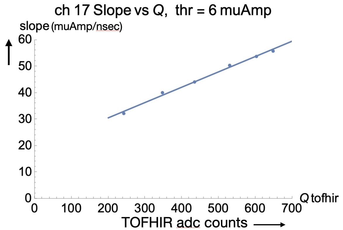
Figure 7: The mapping from Q- the ADC output- to Slope for a given channel at 6$\mu$Amp threshold.

Assuming the calibration data are taken at several threshold settings we can determine the correlation between slope and Q for every channel, in particular how rapidly the slope develops with increasing Q. If this differs among channels then it is reasonable to expect that channels with a more rapid evolution of slope would have a smaller coefficient. This turns out to be the case as can be seen from Figure 8, where channels with smaller values of AWC clearly have a more rapid development of Slope vs. Q.

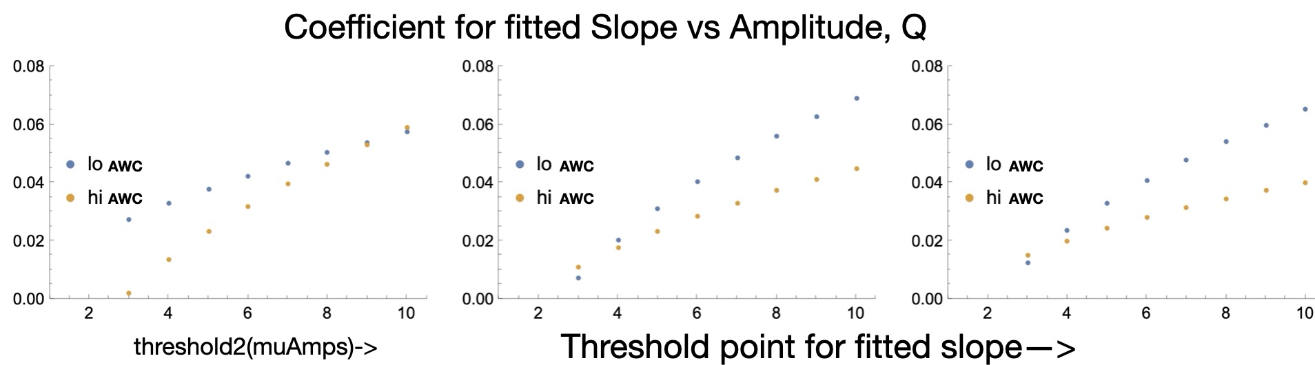
Figure 8: The variation in AWC obtained from fits to walk vs inverse slope as in Figure 5 (paired as “lo AWC" and "hi AWC") is correlated with the rate of Slope change with Q in calibration data. The coefficient of the line fit as in Figure 7 is plotted at 8 values of threshold. We employ this for refining AWC to account for channel to channel differences.

This observation leads to a more refined prediction of individual channel AWC to be applied as in eqn. 2.4, where we refer to the linear fit in Figure 6(right). Since the rms spread about the linear fit varies by only rms$\sim 13\%$ we now have an acceptable Day-1 calibration once the individual channel slope vs. Q tables are accumulated in situ.

Then, for our particular case of the TOFHIR2C, we use the more precise determination of the walk coefficient obtained from the calibration data set and the fit of Figure 6(right):

$$AWC_{channel}=<rawAWC>-15.8(\frac{1.}{MSlQ_{channel}}-15.6)$$ (4.1)

,where MSlQ_channel is a fit value of the slope dependence on Q for a given channel in calibration data and <rawAWC> is the average value found in this study ($\sim 30\mu$Amp).

Having in hand the fixed AWC for each channel, we apply the linear walk correction for events in a given channel:

$$t_{corrected,event}=t_{threshold,event}-AWC\times\frac{1.}{Slope_{event}}$$ (4.2)

,utilizing the Amplitude (Q) measured in the event and the mapping to Slope from the calibration lookup table.

5 Discussion

Equations 4.1 and 4.2 provide the walk calibration for the particular TOFHIR2C based system that we have been studying illustrated in Figure 9.

In using this calibration it should be noted that the calibration is applied in regular data taking with input only from two data words per channel

$$t_{threshold1},Q$$ (5.1)

the walk correction to the time at threshold is completely determined from the earlier calibration data which provided the mapping from Q to Slope for the event. In contrast the same coefficient, AWC, is applied to all events of a given channel.

The procedure during normal data taking is:

• obtain the two data words in eqn. 5.1

• obtain the corresponding Slope for the measured Q from the calibration lookup table

• apply the linear form in eqn 4.2 using the previously determined AWC- which is constant for each channel

Figure 9: Application of eqn 4.2 to a typical channel.

6 Conclusion and Acknowledgement

We have demonstrated that the use of dual threshold to measure pulse slope at threshold can provide an early calibration (a simple linear correction term) for walk -even in a system which departs significantly from linear response.

The aim of this exercise has been to show that the initial crucial walk calibration for large timing systems could be obtained with a very restrictive data set- ie an unbiased sample containing only information internal to the system. More sophisticated data including information from the full event- providing a t₀ reference - would nevertheless be useful to recover possible channel-to-channel offsets due to propagation delays, etc. But this will be greatly simplified having removed walk from the data.

We wish to acknowledge our LIP colleagues- M. Gallinaro for a careful reading of the manuscript and the folks at PETsys, SA for making their test stand available to us. This work was partially supported, through Fermilab, by the US-CMS upgrade program.

References

- [1] for an overview of past (and future) colliders see: V. Shiltsev and F. Zimmerman, "Modern and future colliders", Rev. Mod. Phys. 93, 15006(2021)
- [2] M. Goncharov et al, “The Timing System for the CDF electromagnetic Calorimeters", Nima.2006.06.11
- [3] “PID performance of the ALICE-TOF detector at Run 2", N. Jacazio in Proceedings of LHCP2018, https://pos.sissa.it/321/232/.
- [4] Chapter No. 17 “Radiation Detection and Measurements", Glenn T. Knoll, Third edition (2000), John Wiley. Pulse Processing.
- [5] CMS Collaboration, “A MIP Timing Detector for the CMS Phase-2 Upgrade". Technical Report CERN-LHCC-2019-003. CMS-TDR-020, CERN, Geneva, 2019 and “A High-Granularity Timing Detector for the ATLAS Phase-II Upgrade", CERN-LHCC-2020-007; ATLAS-TDR-031
- [6] E. Albuquerque et al., “TOFHIR2: The readout ASIC of the CMS Barrel MIP Timing Detector", arxiv:2404.01208
- [7] S. White, “Signal processing to reduce dark noise impact in precision timing", Journal of Instrumentation, Volume 18, July 2023.
- [8] L. Vandamme et al., “1/f Noise in MOS Devices, mobility or number fluctuations?" IEEE Vol 41, no. 11 p. 1936 (1994)
- [9] S. White, “Initial Calibration of Large Timing Arrays for the LHC", https://arxiv.org/pdf/2405.08191.
- [10] F. Addesa et al. “Optimization of LYSO crystals and SiPM parameters for the CMS MIP timing detector", Journal of Instrumentation, Volume 19, p 12020.
- [11] S. White “Experimental challenges of the European Strategy for Particle Physics", Proc. Int. Conf. on Calorimetry for the High Energy Frontier (CHEF 2013).
- [12] S. White, “RD for a Dedicated Fast Timing Layer in the CMS Endcap Upgrade", in Proceedings of Workshop on picosecond photon sensors for physics and medical applications, Clermont-Ferrand, France, 12-14 March 2014, Acta Phys. Polon. B Proc. Suppl. 7 (2014) 743.