Test of partial effects for Fréchet regression on Bures-Wasserstein manifolds

Abstract

We propose a novel test for assessing partial effects in Fréchet regression on Bures–Wasserstein manifolds. Our approach employs a sample-splitting strategy: the first subsample is used to fit the Fréchet regression model, yielding estimates of the covariance matrices and their associated optimal-transport maps, while the second subsample is used to construct the test statistic. We prove that this statistic converges in distribution to a weighted mixture of chi-squared components, where the weights correspond to the eigenvalues of an integral operator defined by an appropriate RKHS kernel. We establish that our procedure achieves the nominal asymptotic size and demonstrate that its worst-case power converges uniformly to one. Through extensive simulations and a real data application, we illustrate the test’s finite-sample accuracy and practical utility.

1 Introduction

In many modern applications, positive definite matrices are often used to summarize the marginal covariance structure among sets of variables. Examples include medical imaging (Dryden et al., 2009; Fillard et al., 2007), neuroscience (Friston, 2011; Kong et al., 2020; Hu et al., 2021) and gene coexpression analysis in single cell genomics. A central challenge in these fields is how to perform regression analysis where the covariance matrix serves as the outcome variable in relation to a set of Euclidean covariates and how to test for the association between these matrix and covariates.

Several regression approaches for covariance matrix outcomes have been proposed. Chiu et al. (1996) developed a method that models the elements of the logarithm of the covariance matrix as a linear function of the covariates, but this approach requires estimating a large number of parameters. Hoff & Niu (2012) proposed a regression model where the covariance matrix is expressed as a quadratic function of the explanatory variables. Zou et al. (2017) linked the matrix outcome to a linear combination of similarity matrices derived from the covariates and examined the asymptotic properties of different estimators under this framework. Xu & Li (2025) introduced Fréchet regression with covariate matrix as the outcome. They further developed a formal statistical test for the overall association between covariance matrices and a Euclidean vector of covariates.

Beyond global test for no effect of covariates on covariance matrix, it is often necessary to test the effect for just a single predictor or a subset of them while conditioning on other covariates or confounding variables. For example, in analysis of single cell data, we are interested testing the association between gene co-expression matrix and a covariate of interest conditioning on the proportion of a particular cell type.

In this paper, we develop a novel test for partial effects for Fréchet regression on Bures-Wasserstein manifolds, extending the framework of Xu & Li (2025). Our approach employs sample splitting: the first subsample is used to fit the Fréchet regression model and obtain estimates of covariance matrices along with their optimal transport maps, while the second subsample constructs the test statistic. We prove that this statistic converges to a weighted mixture of chi-squared distributions, where the weights are eigenvalues of an integral operator induced by an appropriate RKHS kernel. We establish that our test achieves the nominal asymptotic size and demonstrate that its worst-case power converges uniformly to one.

2 Problem formulation

2.1 Fréchet regression on Bures-Wasserstein manifold

The Fréchet regression model (Petersen & Müller, 2019) generalizes classical linear regression to arbitrary metric spaces by relying solely on distance rather than linear structure. A key example is the Bures-Wasserstein manifold of symmetric positive-definite (SPD) matrices ${\cal S}_{d}^{++}$, equipped with the Wasserstein distance

$$W(A,B)=\left[\mathop{\mathrm{tr}}{A}+\mathop{\mathrm{tr}}{B}-2\mathop{\mathrm{tr}}\left(A^{1/2}BA^{1/2}\right)^{1/2}\right]^{1/2},\quad\text{for any }A,B\in{\cal S}_{d}^{++}$$

Given a random covariate-response pair $(X,Q)\in\mathbb{R}^{p}\times{\cal S}_{d}^{++}$, the model is based on the conditional Fréchet mean:

$$\mathbb{E}_{\text{Fr\'{e}chet}}\left[Q|X=x\right]:=\mathop{\mathrm{argmin}}_{S\in{\cal S}_{d}^{++}}\mathbb{E}_{Y|X=x}\left[W^{2}(S,Q)|X=x\right]$$

The following lemma, proved by Kroshnin et al. (2021), ensures existence and uniqueness under mild moment conditions.

Lemma 2.1.

On the Bures-Wasserstein manifold $({\cal S}_{d}^{++},W)$, the following hold: (i) If $\mathbb{E}\mathop{\mathrm{tr}}Q<+\infty$, then the Fréchet mean $\mathbb{E}_{\text{Fr\'{e}chet}}Q$ exists uniquely. (ii) If $\mathbb{E}[\mathop{\mathrm{tr}}Q|X=x]<+\infty$, then the conditional Fréchet mean $\mathbb{E}_{\text{Fr\'{e}chet}}\left[Y|X=x\right]$ exists uniquely.

Denoting $Q^{*}(x):=\mathbb{E}_{\mathrm{\text{Fr\'{e}chet}}}\left[Q|X=x\right]$, the Fréchet regression model assumes that

$$Q^{*}(x)=\mathop{\mathrm{argmin}}_{S\in{\cal S}_{d}^{++}}F(x,S),\quad\text{where }F(x,S):=\mathbb{E}_{(X,Q)}\left[w(x,X)W^{2}(S,Q)\right]$$ (1)

with weight function $w$ defined as

$$w(x,X)=1+(x-\mu)^{\top}\Sigma^{-1}(X-\mu),\quad\mu=\mathbb{E}X,\;\ \Sigma=\operatorname{Var}(X)$$

While $Q^{*}(x)$ generally lacks a closed-form expression, it reduces to linear regression on matrix square roots when $Q$ is concentrated on commuting matrices (Xu & Li, 2025).

Given observations $\left\{(X_{i},Q_{i})\right\}_{i=1}^{n}$, we consider the natural estimator

$$\widehat{Q}_{n}(x):=\mathop{\mathrm{argmin}}_{S\in{\cal S}_{d}^{++}}\frac{1}{n}\sum_{i=1}^{n}w_{n}(x,X_{i})W^{2}(S,Q_{i}),\quad w_{n}(x,X_{i}):=1+(x-\mkern 1.5mu\overline{\mkern-1.5muX\mkern-1.5mu}\mkern 1.5mu)^{\top}\widehat{\Sigma}_{n}^{-1}(X_{i}-\mkern 1.5mu\overline{\mkern-1.5muX\mkern-1.5mu}\mkern 1.5mu)$$ (2)

with $\mkern 1.5mu\overline{\mkern-1.5muX\mkern-1.5mu}\mkern 1.5mu=n^{-1}\sum_{i=1}^{n}X_{i}$ and $\widehat{\Sigma}_{n}=n^{-1}\sum_{i=1}^{n}(X_{i}-\mkern 1.5mu\overline{\mkern-1.5muX\mkern-1.5mu}\mkern 1.5mu)(X_{i}-\mkern 1.5mu\overline{\mkern-1.5muX\mkern-1.5mu}\mkern 1.5mu)^{\top}$ . Xu & Li (2025) established uniform convergence of this estimator to $Q^{*}(x)$ and developed a statistical test for the global null hypothesis $H_{0}:Q(x)=Q^{*}_{0}$ for any $x$.

We now consider a partitioned vector covariate $\mathbb{R}^{p}\ni X=(Y,Z)$ where $Y\in\mathbb{R}^{p_{1}}$, $p_{1}\leq p$. Our interest lies in testing for the partial effect of $Z$ on $Q$ given $Y$. The null hypothesis can be formulated as: for all $y\in\mathbb{R}^{p_{1}}$ and $z,\widetilde{z}\in\mathbb{R}^{p-p_{1}}$,

$${\cal H}_{0}:Q^{*}(y,z)=Q^{*}(y,\widetilde{z}).$$ (3)

To develop our test statistic, we require some additional notation. We use $\left[n\right]$ to denote $\left\{1,\ldots,n\right\}$. We denote by $T_{Q}^{S}$ the optimal transport map from $Q$ to $S$ and by $dT_{Q}^{S}$ its differential with respect to $Q$. See Xu & Li (2025) for details on these objects.

2.2 Assumptions

The assumptions needed for partial testing are identical to those in Xu & Li (2025), which we summarize here for completeness. Assumption 2.2, 2.2 below impose light tail conditions on $X$ and boundedness conditions on $Q$. Assumption 2.2, 2.2 specify conditions on the global and local behavior of $F(x,\cdot)$ around its minimizer $Q^{*}(x)$. See Xu & Li (2025) for detailed discussions. The covariate $X$ is sub-Gaussian with $\left\|X\right\|_{\psi_{2}}\leq C_{\psi_{2}}$ and $\lambda_{\min}(\Sigma)\geq c_{\Sigma}$ for some constants $C_{\psi_{2}},c_{\Sigma}>0$.

Given $X=x\in\operatorname{supp}X$, the eigenvalues of $Q$ are bounded away from $0$ and infinity in the sense that

$$\mathbb{P}\left(Q\in{\cal S}_{d}\left(\gamma_{\Lambda}(\left\|x-\mu\right\|)^{-1},\gamma_{\Lambda}(\left\|x-\mu\right\|)\right)|X=x\right)=1$$

where $\gamma_{\Lambda}:\mathbb{R}^{+}\to\mathbb{R}^{+}$ is defined by $\gamma_{\Lambda}(t):=c_{\Lambda}\left(t\vee 1\right)^{C_{\Lambda}}$ for some constants $c_{\Lambda}\geq 1$ and $C_{\Lambda}\geq 0$.

The Fréchet regression model (1) holds for all $x\in\text{supp}(X)$.

For any $x\in\operatorname{supp}X$, the function $F(x,\cdot):{\cal S}_{d}^{++}\to\mathbb{R}$ has a unique minimizer. Moreover, there exist constants $\alpha_{F}\geq 1$ and $\delta_{F}>0$ such that for any $x\in\operatorname{supp}X$ and any $0\leq\delta\leq\delta_{F}\leq\Delta$,

$$\inf\left\{F(x,S)-F(x,Q^{*}(x)):\delta\leq\left\|S-Q^{*}(x)\right\|_{\mathrm{F}}\leq\Delta\right\}\geq\frac{\delta^{\alpha_{F}}}{\gamma_{F}(\left\|x-\mu\right\|,\Delta)}$$

where $\gamma_{F}:\mathbb{R}^{+}\times\mathbb{R}^{+}\to\mathbb{R}^{+}$ is defined by $\gamma_{F}(t_{1},t_{2})=c_{F}\left(t_{1}\vee 1\right)^{C_{F}}\left(t_{2}\vee 1\right)^{C_{F}}$ for constants $c_{F}\geq 1,C_{F}\geq 0$.

For any $x\in\operatorname{supp}X$, consider the symmetric linear operator

$$\mathbb{E}\left(-w(x,X)dT_{Q^{*}(x)}^{Q}\right):{\cal S}_{d}\to{\cal S}_{d},$$

which is the second differential of $F(x,\cdot)$ at $Q^{*}(x)$. This operator has a lower bound for its minimum eigenvalue given by:

$$\lambda_{\min}\left(-\mathbb{E}w(x,X)dT_{Q^{*}(x)}^{Q}\right) \geq\frac{1}{\gamma_{\lambda}(\left\|x-\mu\right\|)}$$

where $\gamma_{\lambda}:\mathbb{R}^{+}\to\mathbb{R}^{+}$ is defined by $\gamma_{\lambda}(t):=c_{\lambda}\left(t\vee 1\right)^{C_{\lambda}}$ for constants $c_{\lambda}\geq 1$ and $C_{\lambda}\geq 0$.

2.3 Test statistic

To test the null hypothesis (3), we employ sample splitting by dividing the data into two halves. Given $n\in\mathbb{N}$, let $n_{1}=\lceil{n/2}\rceil$ and $n_{2}=n-n_{1}$. Let $\mkern 1.5mu\overline{\mkern-1.5muX\mkern-1.5mu}\mkern 1.5mu^{(1)},\widehat{\Sigma}^{(1)}$ denote sample mean and covariance from the first $n_{1}$ samples, and $\mkern 1.5mu\overline{\mkern-1.5muX\mkern-1.5mu}\mkern 1.5mu^{(2)},\widehat{\Sigma}^{(2)}$ those from the last $n_{2}$ samples. Define the estimator based on the first half as

$$\widehat{Q}_{n_{1}}^{(1)}(x)=\mathop{\mathrm{argmin}}_{S\in{\cal S}_{d}^{++}}\frac{1}{n_{1}}\sum_{i=1}^{n_{1}}w_{n_{1}}^{(1)}(x,X_{i})W^{2}(S,Q_{i}).$$

with weight function $w_{n_{1}}^{(1)}(x,X)=1+(x-\mkern 1.5mu\overline{\mkern-1.5muX\mkern-1.5mu}\mkern 1.5mu^{(1)})[\widehat{\Sigma}^{(1)}]^{-1}(X-\mkern 1.5mu\overline{\mkern-1.5muX\mkern-1.5mu}\mkern 1.5mu^{(1)})$.

The test statistic is defined as

$${\cal T}_{n}=\sum_{k=n_{1}+1}^{n}\left\|\left[-\frac{1}{n_{1}}\sum_{i=1}^{n_{1}}w_{n_{1}}^{(1)}(\widehat{X}_{k},X_{i})dT^{Q_{i}}_{\widehat{Q}_{n_{1}}^{(1)}(\widehat{X}_{k})}\right]\cdot\left[\widehat{Q}_{n_{1}}^{(1)}(X_{k})-\widehat{Q}_{n_{1}}^{(1)}(\widehat{X}_{k})\right]\right\|_{\mathrm{F}}^{2}.$$ (4)

where $\widehat{X}_{k}:=(Y_{k},\widehat{Z}_{k})$, $\widehat{Z}_{k}=\mkern 1.5mu\overline{\mkern-1.5muZ\mkern-1.5mu}\mkern 1.5mu^{(1)}+\widehat{\Sigma}_{21}^{(1)}[\widehat{\Sigma}_{11}^{(1)}]^{-1}(Y_{k}-\mkern 1.5mu\overline{\mkern-1.5muY\mkern-1.5mu}\mkern 1.5mu^{(1)})$.

The test statistic (4) is designed to capture the difference between the Fréchet estimates at $X_{k}$ and $\widehat{X}_{k}$. Here, $\widehat{Z}_{k}$ is the simple linear estimate of $Z_{k}$ given $Y_{k}$, based on the first $n_{1}$ samples. The sufficiency of this naive linear estimate, rather than more sophisticated alternatives, stems from the precise definition of the Fréchet regression model (1) and further illustrates that the Fréchet regression is a generalization of linear regression to general metric spaces. Aside from sample splitting, the test statistic (4) directly generalizes the one proposed by Xu & Li (2025), which was designed for the unconditional case where $z=x$. Specifically, when $z=x$, the weight function $w_{n_{1}}^{(1)}(\widehat{X}_{k},X_{i})$ reduces to $1$, and the correspondence becomes apparent.

In the unconditional case, sample splitting is unnecessary because the associated RKHS kernel exhibits a special decoupling property (see (5)). However, when $\text{dim}(x)>\text{dim}(z)$, the kernel no longer decouples (see Theorem 3.1), necessitating sample splitting. Specifically, we apply the Fréchet estimator $\widehat{Q}_{n_{1}}^{(1)}$ trained on the first half of the data to evaluate on points $\left\{X_{i}\right\}_{i=n_{1}+1}^{n}$ from the second half, thereby eliminating certain dependencies between the estimator and the test points. Our numerical simulations confirm that without sample splitting, the test statistic fails to converge to the null distribution specified in Theorem 3.1. See (6) for the technical reasoning behind sample splitting.

3 Asymptotic results

3.1 Asymptotic null distribution

We now establish the limiting distribution of our test statistic under the null hypothesis.

Theorem 3.1.

Suppose Assumption 2.2-2.2 hold. Under the null hypothesis (3), the test statistic ${\cal T}_{n}$ converges in distribution to

$${\cal T}_{n}\xrightarrow{d}\sum_{i=1}^{\infty}\lambda_{i}w_{i},$$

where $\{w_{i}\}_{i\geq 1}$ are independent $\chi_{1}^{2}$ random variables, and $\left\{\lambda_{i}\right\}_{i\geq 1}$ are the eigenvalues of the integral operator with kernel

$${\cal K}(x,Q;x^{\prime},Q^{\prime})=\mathbb{E}_{X}\left\langle\tau(x,Q;X),\tau(x^{\prime},Q^{\prime};X)\right\rangle$$

The influence function $\tau:\mathbb{R}^{p}\times{\cal S}_{d}^{++}\times\mathbb{R}^{p}\to\mathbb{R}^{d\times d}$ is given by

$$\tau(x,Q;X) =\tau_{0}(x,Q;X)-\tau_{1}(x,Q;X)+A(X)\tau_{0}(x,Q;X)$$

where the components are defined as follows

$$\tau_{0}(x,Q;X) =\vec{X}^{\top}\vec{\Sigma}^{-1}\vec{x}\left(T^{Q}_{Q^{*}(X)}-I_{d}\right)-\left[\vec{X}^{\top}\vec{\Sigma}^{-1}\left(\vec{x}\vec{x}^{\top}-\vec{\Sigma}\right)\vec{\Sigma}^{-1}\otimes\mathop{\mathrm{id}}\right]\times\left[\mathbb{E}^{\prime\prime}\vec{X}^{\prime\prime}\otimes\left(T^{Q^{\prime\prime}}_{Q^{*}(X)}-I_{d}\right)\right]$$

$$\tau_{1}(x,Q;X) =\vec{Y}^{\top}\vec{\Sigma}_{11}^{-1}\vec{y}\left(T^{Q}_{Q^{*}(X)}-I_{d}\right)-\left[\vec{Y}^{\top}\vec{\Sigma}_{11}^{-1}\left(\vec{y}\vec{y}^{\top}-\vec{\Sigma}_{11}\right)\vec{\Sigma}_{11}^{-1}\otimes\mathop{\mathrm{id}}\right]\times\left[\mathbb{E}^{\prime\prime}\vec{Y}^{\prime\prime}\otimes\left(T^{Q^{\prime\prime}}_{Q^{*}(X)}-I_{d}\right)\right]$$

$$A(X) =\left[\mathbb{E}^{\prime\prime}\left(w(X,X^{\prime\prime})-w(\widetilde{X},X^{\prime\prime})\right)dT^{Q^{\prime\prime}}_{Q^{*}(X)}\right]\cdot\left[-\mathbb{E}^{\prime\prime}w(X,X^{\prime\prime})dT^{Q^{\prime\prime}}_{Q^{*}(X)}\right]^{-1}$$

where $\widetilde{X}:=(Y,\mu_{Z}+\Sigma_{21}\Sigma_{11}^{-1}(Y-\mu_{Y}))$ denotes the imputed covariate vector, and $\mathbb{E}^{\prime\prime}$ are taken over independent copies $(X^{\prime\prime},Q^{\prime\prime})$ of $(X,Q)$.

We defer the proof to the Supplementary Material . With a slight abuse of notation, we also use ${\cal K}$ to denote the integral operator induced by the kernel ${\cal K}$. Under Assumptions 2.2 and 2.2, together with Lemma 13 in the Supplementary Material, we have $\mathop{\mathrm{tr}}{\cal K}=\mathbb{E}_{(X,Q)\otimes X^{\prime}}\left\|\tau(X,Q;X^{\prime})\right\|_{\mathrm{F}}^{2}<\infty$ where $X^{\prime}$ is an independent copy of $X$. Hence ${\cal K}$ is a trace-class operator on $L^{2}(\mathbb{R}^{p}\times{\cal S}_{d}^{++})$. Moreover, since $\mathbb{E}\sum_{i=1}^{\infty}\lambda_{i}w_{i}=\mathop{\mathrm{tr}}{\cal K}$, the series $\sum_{i=1}^{\infty}\lambda_{i}w_{i}$ is a well-defined non-negative random variable with finite expectation.

In the unconditional case $z=x$, we have under the null hypothesis:

$$\tau(x,Q;X)=\tau_{0}(x,Q;X)=\vec{X}^{\top}\vec{\Sigma}^{-1}\vec{x}\left(T^{Q}_{Q^{*}(\mu)}-I_{d}\right)$$ (5)

Here the $(x,Q)$ and $X$ components decouple, yielding a product kernel:

$${\cal K}(x,Q;x^{\prime},Q^{\prime})=\left\langle\vec{x},\vec{\Sigma}^{-1}\vec{x}^{\prime}\right\rangle\cdot\left\langle T^{Q}_{Q^{*}(\mu)}-I_{d},T^{Q^{\prime}}_{Q^{*}(\mu)}-I_{d}\right\rangle$$

By leveraging the spectral properties of this integral operator, we recover the asymptotic null distribution from Xu & Li (2025). This decoupling property eliminates the need for sample splitting, explaining why the test statistic in Xu & Li (2025) operates on the full sample.

When $\text{dim}(z)<\text{dim}(x)$, the kernel ${\cal K}$ no longer decouples. Without sample splitting, the test statistic

$${\cal T}_{n,\text{full}}:=\sum_{k=1}^{n}\left\|\left[-\frac{1}{n}\sum_{i=1}^{n}w_{n}(\widehat{X}_{k},X_{i})dT^{Q_{i}}_{\widehat{Q}_{n}(\widehat{X}_{k})}\right]\cdot\left[\widehat{Q}_{n}(X_{k})-\widehat{Q}_{n}(\widehat{X}_{k})\right]\right\|_{\mathrm{F}}^{2}$$

can be approximated by

$${\cal T}_{n,\text{full}}\approx\frac{1}{n}\sum_{i,j\in[n]}{\cal K}_{n}(X_{i},Q_{i};X_{j},Q_{j})$$

where ${\cal K}_{n}$ is a data-dependent kernel. The complex dependence between ${\cal K}_{n}$ and $\left\{(X_{i},Q_{i})\right\}_{i\in[n]}$ prevents us from deriving the asymptotic null distribution of ${\cal T}_{n,\text{full}}$. Indeed, our simulations confirm that the test statistic ${\cal T}_{n,\text{full}}$ fails to converge to the null distribution specified in Theorem 3.1. Sample splitting eliminates this dependence by ensuring that

$${\cal T}_{n}\approx\frac{1}{n_{1}}\sum_{i,j\in[n_{1}]}{\cal K}_{n}^{(2)}(X_{i},Q_{i};X_{j},Q_{j})$$ (6)

where ${\cal K}_{n}^{(2)}$ depends only on the second-half of data $\left\{(X_{i},Q_{i})\right\}_{i=n_{1}+1}^{n}$. This independence between the kernel and the summation indices enables us to derive the asymptotic null distribution of ${\cal T}_{n}$; see Supplementary Material for more details.

To estimate the eigenvalues $\{\lambda_{j}\}_{j\geq 1}$, we employ a kernel matrix approach. For notational clarity, we first introduce the empirical covariance matrices $\Xi^{(1)}:=n_{1}^{-1}\sum_{i=1}^{n_{1}}\vec{X}_{i}\vec{X}_{i}^{\top}$ and $\Xi^{(1)}_{11}=n_{1}^{-1}\sum_{i=1}^{n_{1}}\vec{Y}_{i}\vec{Y}_{i}^{\top}$. The eigenvalues estimates $\{\widehat{\lambda}_{j}\}_{j=1}^{n_{2}}$ are obtained as the eigenvalues of the $n_{2}\times n_{2}$ kernel matrix

$$\boldsymbol{K}_{n}:=\frac{1}{n_{2}}(\widehat{{\cal K}}_{n}^{(1)}(X_{i},Q_{i};X_{j},Q_{j}))_{i,j\in n_{1}+[n_{2}]}\in\mathbb{R}^{n_{2}\times n_{2}}$$

where the kernel function $\widehat{{\cal K}}_{n}^{(1)}$ is computed using the first half of data:

$$\widehat{{\cal K}}_{n}^{(1)}(x,Q;x^{\prime},Q^{\prime})=\frac{1}{n_{1}}\sum_{k=1}^{n_{1}}\left\langle\widehat{\tau}(x,Q;X_{k}),\widehat{\tau}(x^{\prime},Q^{\prime};X_{k})\right\rangle$$

The function $\widehat{\tau}$ here captures the influence of each observation and is defined as

$$\widehat{\tau}(x,Q;X) =\widehat{\tau}_{0}(x,Q;X)-\widehat{\tau}_{1}(x,Q;X)+\widehat{A}(X)\widehat{\tau}_{0}(x,Q;X)$$

$$\widehat{\tau}_{0}(x,Q;X) =\vec{X}^{\top}[\Xi^{(1)}]^{-1}\vec{x}\left(T^{Q}_{\widehat{Q}_{n_{1}}^{(1)}(X)}-I_{d}\right)$$

$$-\left[\vec{X}^{\top}[\Xi^{(1)}]^{-1}\left(\vec{x}\vec{x}^{\top}-\Xi^{(1)}\right)[\Xi^{(1)}]^{-1}\otimes\mathop{\mathrm{id}}\right]\times\left[\frac{1}{n_{1}}\sum_{i=1}^{n_{1}}\vec{X}_{i}\otimes\left(T^{Q_{i}}_{\widehat{Q}_{n_{1}}^{(1)}(X)}-I_{d}\right)\right]$$

$$\widehat{\tau}_{1}(x,Q;X) =\vec{Y}^{\top}[\Xi^{(1)}_{11}]^{-1}\vec{y}\left(T^{Q}_{\widehat{Q}_{n_{1}}^{(1)}(X)}-I_{d}\right)$$

$$-\left[\vec{Y}^{\top}[\Xi^{(1)}_{11}]^{-1}\left(\vec{y}\vec{y}^{\top}-\Xi^{(1)}_{11}\right)[\Xi^{(1)}_{11}]^{-1}\otimes\mathop{\mathrm{id}}\right]\times\left[\frac{1}{n_{1}}\sum_{i=1}^{n_{1}}\vec{Y}_{i}\otimes\left(T^{Q_{i}}_{\widehat{Q}_{n_{1}}^{(1)}(X)}-I_{d}\right)\right]$$

$$\widehat{A}(X) =\left[\frac{1}{n_{1}}\sum_{i=1}^{n_{1}}\left(w_{n_{1}}^{(1)}(X,X_{i})-w_{n_{1}}^{(1)}(\widehat{X},X_{i})\right)dT^{Q_{i}}_{\widehat{Q}_{n_{1}}^{(1)}(X)}\right]\left[-\frac{1}{n_{1}}\sum_{i=1}^{n_{1}}w_{n_{1}}^{(1)}(X,X_{i})dT^{Q_{i}}_{\widehat{Q}^{(1)}_{n_{1}}(X)}\right]^{-1}$$

with $\widehat{X}:=(Y,\mkern 1.5mu\overline{\mkern-1.5muZ\mkern-1.5mu}\mkern 1.5mu^{(1)}+\widehat{\Sigma}_{21}^{(1)}[\widehat{\Sigma}_{11}^{(1)}]^{-1}(Y-\mkern 1.5mu\overline{\mkern-1.5muY\mkern-1.5mu}\mkern 1.5mu^{(1)}))$.

Given the eigenvalue estimates $\{\widehat{\lambda}_{j}\}_{j=1}^{n_{2}}$, let $\widehat{q}_{1-\alpha}$ denote the $(1-\alpha)$-quantile of $\sum_{j=1}^{n_{2}}\widehat{\lambda}_{j}w_{j}$. We define our level-$\alpha$ test $\Phi_{n,\alpha}$ as $\Phi_{n,\alpha}:=\boldsymbol{1}\left({\cal T}_{n}>\widehat{q}_{1-\alpha}\right)$. The following theorem establishes the asymptotic validity of our test.

Theorem 3.2.

Suppose Assumption 2.2-2.2 hold. Under the null hypothesis (3), the test $\Phi_{n,\alpha}$ achieves the nominal level asymptotically:

$$\lim_{n\to\infty}\mathbb{P}\left({\cal T}_{n}>\widehat{q}_{1-\alpha}\right)=\alpha$$

See the Supplementary Material for the proof.

3.2 Asymptotic power of the proposed test

We now analyze the power of the test $\Phi_{n,\alpha}$ against a sequence of alternative hypotheses. The analysis is based on the following uniform convergence result for $\widehat{Q}_{n}(\widehat{x})$, which establishes that $\widehat{Q}_{n}(\widehat{x})$ is a uniformly consistent estimator of the population quantity $Q^{*}(\widetilde{x})$.

Theorem 3.3.

Let $0\leq L_{n}\leq C_{L}(\log n)^{1/2}$ for some constant $C_{L}>0$. Under Assumption 2.2-2.2 hold, for any arbitrarily large constant $\tau>0$, with probability at least $1-C_{3}n^{-\tau}$,

$$\sup_{\left\|x-\mu\right\|\leq L_{n}}\left\|\widehat{Q}_{n}(\widehat{x})-Q^{*}(\widetilde{x})\right\|_{\mathrm{F}}\leq C_{1}\frac{\log^{C_{2}}{n}}{\sqrt{n}}$$

for some constants $C_{1},C_{2},C_{3}>0$ independent of $n$. Here $x=(y,z)$, $\widehat{x}=(y,\widehat{z})$ with $\widehat{z}=\mkern 1.5mu\overline{\mkern-1.5muZ\mkern-1.5mu}\mkern 1.5mu^{(1)}+\widehat{\Sigma}_{21}^{(1)}[\widehat{\Sigma}_{11}^{(1)}]^{-1}(y-\mkern 1.5mu\overline{\mkern-1.5muY\mkern-1.5mu}\mkern 1.5mu^{(1)})$ denotes the observation with imputed $Z$-component, and $\widetilde{x}=(x,\widetilde{z})$ with $\widetilde{z}=\mu_{Z}+\Sigma_{21}\Sigma_{11}^{-1}(y-\mu_{Y})$ its population counterpart.

The proof is given in the Supplementary Material.

To characterize the power properties, we first define the hypothesis space. Let $\mathscr{P}$ denote the class of distributions satisfying our regularity conditions:

$$\mathscr{P}:=\left\{\mathbb{P}\in{\cal P}_{2}\left(\mathbb{R}^{p}\times{\cal S}_{d}^{++}\right):\mathbb{P}\text{ satisfies }\text{Assumption }\ref{assumption: X}-\ref{assumption: minimizer_local}\right\}$$

We consider alternatives where the conditional independence fails by at least a specified amount. Define the alternative hypothesis class

$${\cal H}_{1,n}:\mathbb{P}\in\mathscr{P}_{F}(a_{n}):=\left\{\widetilde{\mathbb{P}}\in\mathscr{P}:\mathbb{E}_{(X,Q)\sim\widetilde{\mathbb{P}}}\left\|Q^{*}(X)-Q^{*}\left((Y,\mu_{Z}+\Sigma_{21}\Sigma_{11}^{-1}(Y-\mu_{Y}))\right)\right\|_{\mathrm{F}}^{2}\geq a_{n}^{2}\right\}$$

The following theorem establishes uniform consistency of our test against these alternatives.

Theorem 3.4.

Consider a sequence of alternative hypotheses ${\cal H}_{1,n}$ with $a_{n}\gtrsim n^{\alpha_{F}-1/2}$ for some constant $\alpha_{F}>0$. Then the worst-case power converges uniformly to 1:

$$\lim_{n\to\infty}\inf_{\mathbb{P}\in\mathscr{P}_{F}(a_{n})}\mathbb{P}\left({\cal T}_{n}>\widehat{q}_{1-\alpha}\right)=1$$

The proof is given in the Supplementary Material.

4 Numerical simulations

In this section, we present numerical experiments to demonstrate the effectiveness of our proposed test. We compute the estimator (2) using the Riemannian gradient descent algorithm from Xu & Li (2025). To assess the test’s performance, we conduct 200 independent Monte Carlo trials for each simulation setting. We consider two illustrative examples that follow the Fréchet regression model. Example 4.1 examines the case where covariance matrices share a common eigenspace and commute, which simplifies the Fréchet regression to a linear regression on matrix square roots. In contrast, Example 4.2 explores the more complex non-commutative setting where covariance matrices possess distinct eigenspaces.

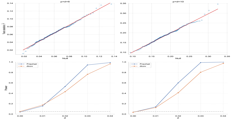
(a) Example 4.1 (commutative case) with $n=200$ and $(p_{y},p_{z},d)\in\{(3,3,6),(5,5,10)\}$

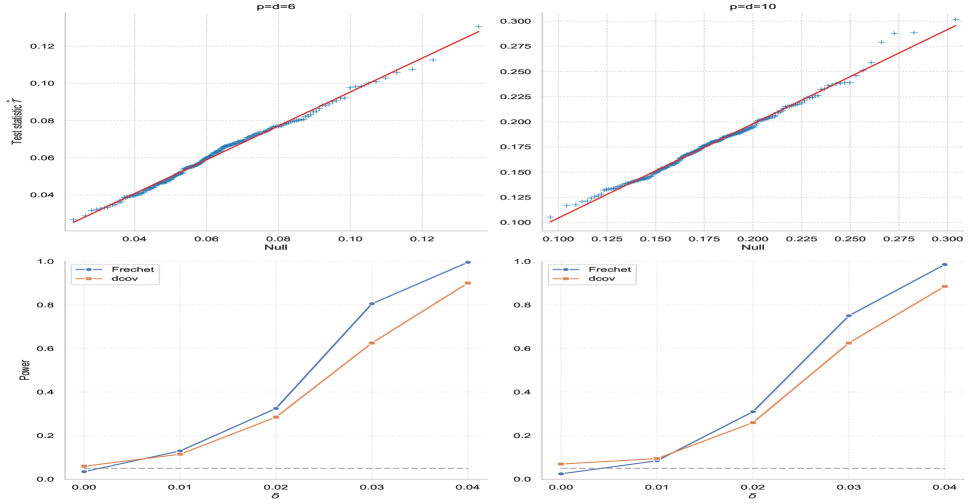
(b) Example 4.2 (non-commutative case) with $n=200$ and $(p_{y},p_{z},d)\in\{(3,3,6),(5,5,10)\}$

Figure 1: Q-Q plots of $\mathcal{T}_{n}$ under ${\cal H}_{0}$ against its asymptotic null distribution, and empirical power curves as a function of the effect size $\delta_{z}$.

Example 4.1.

Let $\left\{X_{i}=\left(X_{i1}\;\ \cdots\;\ X_{ip}\right),i\in[n]\right\}$ be i.i.d. random covariates in $\mathbb{R}^{p}$ with $X_{i}\sim\mathrm{Uniform}[-1,1]^{p}$. The response matrices $Q_{1},\ldots,Q_{n}\in\mathbb{R}^{d\times d}$ are generated as:

$$Q_{i}=UV_{i}f(X_{i};\delta)^{2}V_{i}U^{\top}$$

Here $U$ and $\left\{X_{i},V_{i}\right\}_{i\in[n]}$ are independent, and $f(\cdot;\delta):\mathbb{R}^{p}\to\mathbb{R}^{d\times d}$ is a mapping from $\mathbb{R}^{p}$ to diagonal matrices defined by:

$$x=\left(y\;\ z\right)\mapsto f(x;\delta)=\left(f(x;\delta)_{kl}\right)_{k,l\in[d]},$$

where $y\in\mathbb{R}^{p_{y}}$, $z\in\mathbb{R}^{p_{z}}$ with $p_{y}+p_{z}=p$, and

$$f(x;\delta)_{kk}=1.5+\frac{k}{2}+0.1\sum_{j=1}^{p_{y}}y_{j}+\delta_{z}\sum_{l=1}^{p_{z}}z_{l},$$

Here $\delta_{z}\in(-2p^{-1},2p^{-1})$ is a parameter that controls the deviation from the null hypothesis (3), with $\delta_{z}=0$ corresponding to the null. $U\in{\cal O}_{d}$ is a random orthogonal matrix following the Haar measure. $V_{i}\in\mathbb{R}^{d}$ is a random diagonal matrix with i.i.d. diagonal entries $V_{i,kk}\sim\mathrm{Uniform}[-0.9,1.1]$. It can be verified that the pair $(X,Q)$ satisfies the Fréchet regression model with the conditional expectation $Q^{*}(\cdot)$ satisfying $Q^{*}(X_{i})=Uf(X_{i})^{2}U^{\top}$.

Example 4.2.

Let $X=\left(X_{1}\;\ \cdots\;\ X_{p}\right)$ be a random covariate in $\mathbb{R}^{p}$ with $X\sim\mathrm{Uniform}[-1,1]^{p}$. The response matrix $Q\in\mathbb{R}^{d\times d}$, where $d$ is an even number, is generated as:

$$Q=UVg(X;\delta)^{2}VU^{\top},$$

Here $U,V$ and $X$ are independent, and $g(\cdot;\delta):\mathbb{R}^{p}\to\mathbb{R}^{d\times d}$ is a mapping from $\mathbb{R}^{p}$ to diagonal matrices defined by:

$$x=\left(y\;\ z\right)\mapsto g(x;\delta)=\left(g(x;\delta)_{kl}\right)_{k,l\in[d]},$$

where $y\in\mathbb{R}^{p_{y}}$, $z\in\mathbb{R}^{p_{z}}$ with $p_{y}+p_{z}=p$, and

$$g(x;\delta)_{kk}=1.5+0.5\cdot\lceil k/2\rceil+0.1\sum_{j=1}^{p_{y}}y_{j}+\delta_{z}\sum_{l=1}^{p_{z}}z_{l},$$

with $\lceil{\cdot}\rceil$ denoting the ceiling function, and $\delta_{z}\in(-2p^{-1},2p^{-1})$. $U\in{\cal O}_{d}$ is a random orthogonal matrix with a block-diagonal structure $U=\operatorname{diag}(U^{(1)},\ldots,U^{(\lfloor d/2\rfloor)})$ where $U^{(1)},\ldots,U^{(\lfloor d/2\rfloor)}$ are i.i.d. random $2\times 2$ orthogonal matrices following the Haar measure. $V\in\mathbb{R}^{d}$ is a diagonal matrix with i.i.d. diagonal entries $V_{ii}\sim\mathrm{Uniform}[-0.9,1.1]$. It can be verified that the pair $(X,Q)$ satisfies the Fréchet regression model with $Q^{*}(x)={g(x)}^{2}$.

Using these two examples, we evaluate our test’s performance through Q-Q plots and power analysis. Figure 1 shows Q-Q plots of the test statistic ${\cal T}_{n}$ against its asymptotic null distribution, along with empirical power curves. The Q-Q plots exhibit excellent agreement with the theoretical distribution, following the identity line closely. We compare our test’s power with the distance covariance test (Székely & Rizzo, 2014) for partial correlations, implemented via the Python $\mathrm{dcor}$ package (Ramos-Carreño & Torrecilla, 2023). As our test is specifically designed for Fréchet regression while the distance covariance test is fully nonparametric, as expected we observe superior power in this parametric setting.

5 Application to single cell co-expression analysis

Aging is a complex process of accumulation of molecular, cellular, and organ damage, leading to loss of function and increased vulnerability to disease and death. Nutrient-sensing pathways, namely insulin/insulin-like growth factor signaling and target-of-rapamycin are conserved in various organisms. We are interested in understanding the co-expression structure of 61 genes in this KEGG nutrient-sensing pathways based on the recently published population scale single cell RNA-seq data of human peripheral blood mononuclear cells (PBMCs) from blood samples of over 982 healthy individuals with ages ranging from 20 to 90 (Yazar et al., 2022).

Our analysis focuses on CD4+ naive and central memory T (CD4NC) cells, the most abundant cell type in the dataset. Age-associated changes in CD4 T-cell functionality have been linked to chronic inflammation and decreased immunity (Elyahu et al., 2019). There are a total of 51 genes that are expressed in this cell type. While the Fréchet regression still makes sense when the covariance matrix is potentially degenerate, our theory relies on the strict positive definiteness. Hence, we retain only the genes that have nonzero variances at any age, resulting in a total of $37$ genes. For each individual, we then calculate the sample covariance matrix of these 37 genes based on the observed single cell data, which represents individual-specific gene co-expression network.

Figure 2 displays the top three eigenvalues of the observed covariance matrices alongside the corresponding eigenvalues from the Fréchet regression estimates across different ages, revealing age-related variation in gene co-expression structure. When applying Fréchet regression with age as the sole covariate, the test proposed by Xu & Li (2025) demonstrates a highly significant association between gene co-expression and age with a p-value of 0.00019.

We further investigated whether this association persists after adjusting for CD4NC cell proportion. Specifically, we tested the null hypothesis ${\cal H}_{0}:Q^{*}(y,t)=Q^{*}(y,t^{\prime})$ for any age $t,t^{\prime}$ and cell proportion $y$. This tests whether age effects on gene co-expression remain after controlling for cell proportion variation. Our proposed test yielded a p-value of 0.00082, indicating that the age-gene co-expression association remains significant even after this adjustment.

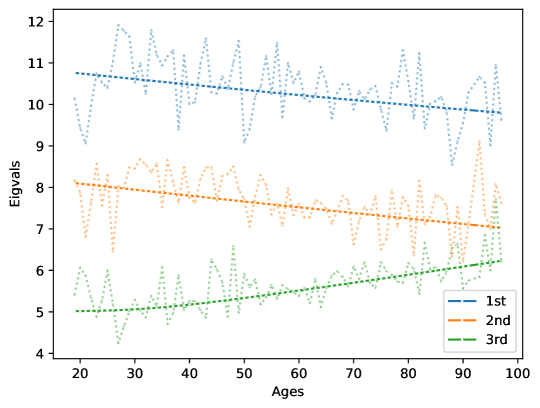
Figure 2: Eigenvalues vs. Age based on sample (dotted lines) and the Fréchet regression estimates (dashed lines) of the covariance matrices.

References

- Chiu et al. (1996) Chiu, T. Y. M., Leonard, T. & Tsui, K.-W. (1996). The Matrix-Logarithmic Covariance Model. Journal of the American Statistical Association 91, 198–210.
- Dryden et al. (2009) Dryden, I. L., Koloydenko, A. & Zhou, D. (2009). Non-Euclidean statistics for covariance matrices, with applications to diffusion tensor imaging. The Annals of Applied Statistics 3, 1102–1123.
- Elyahu et al. (2019) Elyahu, Y., Hekselman, I., Eizenberg-Magar, I., Berner, O., Strominger, I., Schiller, M., Mittal, K., Nemirovsky, A., Eremenko, E., Vital, A., Simonovsky, E., Chalifa-Caspi, V., Friedman, N., Yeger-Lotem, E. & Monsonego, A. (2019). Aging promotes reorganization of the CD4 T cell landscape toward extreme regulatory and effector phenotypes. Science Advances 5, eaaw8330.
- Fillard et al. (2007) Fillard, P., Arsigny, V., Pennec, X., Hayashi, K. M., Thompson, P. M. & Ayache, N. (2007). Measuring brain variability by extrapolating sparse tensor fields measured on sulcal lines. Neuroimage 34, 639–650.
- Friston (2011) Friston, K. J. (2011). Functional and effective connectivity: a review. Brain Connectivity 1, 13–36.
- Hoff & Niu (2012) Hoff, P. D. & Niu, X. (2012). A covariance regression model. Statistica Sinica , 729–753.
- Hu et al. (2021) Hu, W., Pan, T., Kong, D. & Shen, W. (2021). Nonparametric matrix response regression with application to brain imaging data analysis. Biometrics 77, 1227–1240.
- Kong et al. (2020) Kong, D., An, B., Zhang, J. & Zhu, H. (2020). L2rm: Low-rank linear regression models for high-dimensional matrix responses. Journal of the American Statistical Association 115, 403–424.
- Kroshnin et al. (2021) Kroshnin, A., Spokoiny, V. & Suvorikova, A. (2021). Statistical inference for Bures–Wasserstein barycenters. The Annals of Applied Probability 31, 1264–1298.
- Petersen & Müller (2019) Petersen, A. & Müller, H.-G. (2019). Fréchet regression for random objects with Euclidean predictors. The Annals of Statistics 47, 691–719.
- Ramos-Carreño & Torrecilla (2023) Ramos-Carreño, C. & Torrecilla, J. L. (2023). dcor: Distance correlation and energy statistics in Python. SoftwareX 22.
- Székely & Rizzo (2014) Székely, G. J. & Rizzo, M. L. (2014). Partial distance correlation with methods for dissimilarities. The Annals of Statistics 42, 2382–2412.
- Xu & Li (2025) Xu, H. & Li, H. (2025). Wasserstein f-tests for frechet regression on bures-wasserstein manifolds. Journal of Machine Learning Research 26, 1–123.
- Yazar et al. (2022) Yazar, S., Alquicira-Hernandez, J., Wing, K., Senabouth, A., Gordon, M. G., Andersen, S., Lu, Q., Rowson, A., Taylor, T. R. P., Clarke, L., Maccora, K., Chen, C., Cook, A. L., Ye, C. J., Fairfax, K. A., Hewitt, A. W. & Powell, J. E. (2022). Single-cell eqtl mapping identifies cell type–specific genetic control of autoimmune disease. Science 376, eabf3041.
- Zou et al. (2017) Zou, T., Lan, W., Wang, H. & Tsai, C.-L. (2017). Covariance Regression Analysis. Journal of the American Statistical Association 112, 266–281.