Search for Higher Harmonic Signals from Close White Dwarf Binaries in the mHz Band

Abstract

Space-based gravitational wave (GW) detectors, such as LISA, are expected to detect thousands of Galactic close white dwarf binaries emitting nearly monochromatic GWs. In this study, we demonstrate that LISA is reasonably likely to detect higher harmonic GW signals, particularly the $(l,|m|)=(3,3)$ mode, from a limited sample of nearby close white dwarf binaries, even with small orbital velocities $v/c$ of order $10^{-3}$. The amplitudes of these post-Newtonian modes provide robust probes of mass asymmetry in such systems, making them valuable observational targets, especially in mass-transferring binaries. Long-term, coordinated detector operations will further improve the prospects for detecting these informative signals.

Introduction— In the past ten years, LIGO and Virgo detectors have detected over 100 gravitational wave (GW) signals, mainly from binary black holes [1]. Up until just before the mergers, these GW signals are dominated by the mode emitted at twice the orbital frequency, as predicted by the Newtonian quadrupole formula for a circular orbit [2, 3]. In the so-called restricted phase approach, we focus exclusively on this dominant frequency component to facilitate an efficient data analysis [4].

Even from circular binaries, higher harmonic (HH) signals are generated by the post-Newtonian (PN) effect, which is characterized by the PN parameter $\beta\sim v/c$ ($v$: the orbital velocity, $c$: the speed of light) [2, 3]. The amplitudes of the leading order HH terms are suppressed by the factor $\beta$, relative to the Newtonian quadrupole term. The LIGO-Virgo network has already detected HH signals from asymmetric systems, such as GW190412 and GW190814, in the strong gravity regime ($\beta\gtrsim 0.1$) [5, 6]. These detections have significantly improved the estimation of binary parameters (e.g., spins and distances) and strengthened constraints on gravity theories.

Close white dwarf binaries (CWDBs) in our Galaxy are guaranteed GW sources for the future space interferometers such as LISA [7], Taiji [8] and TianQin [9]. Indeed, above 4mHz, LISA is expected to detect $\sim 2000$ detached CWDBs and a similar number of semi-detached CWDBs (AMCVn binaries) which transfer masses from the donors to the accreters [10, 11, 12, 7, 13]. Currently, only three Galactic CWDBs have been identified in the frequency range above $4$ mHz through electromagnetic (EM) observations [14]. However, the number of identified CWDBs is expected to steadily increase as time-domain EM surveys continue to advance.

Given the long radiation reaction timescale, the orbital frequency of a CWDB remains nearly constant. Its gradual frequency drift will be a basic observational target for LISA [7]. Importantly, due to its small PN parameters $\beta=O(10^{-3})$ and the relatively large radii of white dwarfs, not only relativistic effects but also other astrophysical processes could significantly influence the frequency drift of a CWDB. For example, the dissipation rate of orbital energy may be temporarily enhanced by magnetic fields (e.g., [15, 16]; see also [17] for tidal effects). Moreover, an AM CVn binary can exhibit a negative chirp as a result of internal mass transfer [7]. To better understand these complex systems, we should fully exploit the available GW data.

The restricted phase approach appears to be a sufficient method for observing GWs from circular CWDBs. This is primarily due to the significantly smaller PN parameters of CWDBs, compared to the binaries observed by LIGO and Virgo in the strong gravity regime. In fact, the detectability of HH modes in circular CWDBs has been overlooked until now. However, these PN modes are, in principle, sensitive to mass asymmetry. This characteristic plays a critical role, particularly in the long-term evolution and final outcomes of the binaries [18, 7].

In this work, we demonstrate that LISA actually has a good chance to detect the HH modes for several nearby CWDBs. Due to their proximity to the Sun, these binaries will be bright GW sources and will be ideal systems for exploring weak and intriguing signatures not only the HH modes. We also discuss the decomposition scheme for these signatures.

Quadrupole GW Emission— Let us consider a circular CWDB with an orbital frequency $f_{\rm o}$ and the component masses $m_{a}$ and $m_{b}$ ($m_{a}\geq m_{b}$). We define the total mass $m=m_{a}+m_{b}$ and the chirp mass ${\cal M}=(m_{a}m_{b})^{3/5}m^{-1/5}$. In addition, we define the mass difference ratio $\Delta={(m_{a}-m_{b})}/{m}$, which will later become important.

For a circular orbit, the lowest quadrupole radiation is emitted only at the frequency $f_{2}\equiv 2f_{\rm o}$. Its strain signal is expressed as

$$h_{+}^{[0]}=AH_{+}^{[0]},~~~h_{\times}^{[0]}=AH_{\times}^{[0]}$$ (1)

in terms of the amplitude $A$ and the emission pattern functions $H_{{+,\times}}^{[0]}$. In this work, the numbers in the square parentheses (e.g., $h_{+}^{[0]}$) show the PN orders and those in the subscripts (e.g., $f_{2}$) represent the wave frequencies in units of the orbital frequency $f_{\rm o}$.

The amplitude $A$ is given as

$$A\equiv\frac{2{\cal M}^{5/3}G^{5/3}\pi^{2/3}f_{2}^{2/3}}{c^{4}d}$$ (2)

with the gravitational constant $G$ and the distance $d$ to the CWDB. Here, we apply the point-particle approximation and ignore the small correction of order $O[(R/D)^{5}]$, which arises from the deformation of the stars ($R$: stellar radius; $D$: orbital separation) [3] (see also [19] for numerical evaluations showing that the corrections are at most $\sim 1\%$).

In the principle polarization axes, the functions $H_{{+,\times}}^{[0]}$ are given by

$$H_{+}^{[0]} = -(1+\cos^{2}I)\cos 2\Psi=a_{2+}(I)\cos 2\Psi,$$ (3)

$$H_{\times}^{[0]} = -2\cos I\sin 2\Psi=a_{2\times}(I)\sin 2\Psi$$ (4)

with the inclination angle $I$ and the orbital phase $\Psi$ [satisfying $f_{\rm o}={\dot{\Psi}}/(2\pi)$] [2, 3]. In Eqs. (3) and (4), we defined the coefficients $a_{2+}$ and $a_{2\times}$, which correspond to the $(l,|m|)=(2,2)$ modes of the spin-weighted spherical harmonics ${}_{-2}Y_{lm}(I,\Psi)$ [2].

To characterize the total signal strength, we introduce the intensity function $E_{2}(I)$ (see appendix A for detail) by

$$E_{2}(I)\equiv\left[a_{2+}(I)^{2}+a_{2\times}(I)^{2}\right]^{1/2}.$$ (5)

The matched filtering analysis is the standard technique for detecting a regular GW signal characterized by a small number of parameters. For the quadrupole GW from a circular CWDB, considering the response of detectors, the fitting parameters are the amplitude $A$, the sky position, the orientation angles (usually the inclination $I$ and the polarization angle), the initial phase and the GW frequency $f_{2}$ and its time derivatives.

Due to the annual rotation of LISA’s detector plane, the sensitivity to linearly polarized incident GWs are efficiently averaged out (see e.g., [20]). In fact, in the relevant frequency regime, if the integration period $T$ is a multiple of 1yr, the minimum sensitivity to the linearly polarized GWs is estimated to reach 0.89 of their root mean square value [20]. Also counting the numerical factors, we can estimate the signal-to-noise ratio $\rho_{2}$ of the quadrupole radiation as

$$\rho_{2}\simeq\frac{AE_{2}T^{1/2}}{[S_{n}(f_{2})]^{1/2}}$$ (6)

with the effective noise spectrum $S_{n}(f_{2})$ [21].

At present, from EM observations, we have only three Galactic CWDBs at $f_{2}\geq 4$mHz [14]. They are HM Cancri at $f_{2}=6.2$mHz [22, 23], ZTF J1539+5027 at $f_{2}=4.8$mHz [24], and ZTF J0456+3843 at $f_{2}=4.2$mHz [14]. In our study below, except for their distances, we use the first two binaries as representative systems. Their basic parameters are summarized in Table I, including the Galactic coordinates $(l,b)$ with $b=0$ for the disk plane. Below, we briefly introduce the two binaries.

HM Cancri is an AMCVn binary, transferring mass from its donor ($m_{b}$) to its accreter ($m_{a}$), still in the inspiral phase ${\dot{f}}_{\rm o}>0$ [22, 23]. The stability of the mass transfer is considered to depend critically on the asymmetry between $m_{a}$ and $m_{b}$. [18]. The classical stability criterion ($m_{b}/m_{a}\leq 2/3$ [25]) corresponds to $\Delta\geq 1/5$. In contrast to the masses $0.55+0.27\,M_{\odot}$ ($\Delta=0.34$) presented in Table I [26], the best-fit model in [23] is $1.0+0.17\,M_{\odot}$ ($\Delta=0.71$), highlighting the uncertainties in mass estimation even with long-term, extensive EM observations.

Interestingly, at present, without a parallax measurement, the distance $d$ to HM Cancri remains highly uncertain. From its observed proper motion together with a model for the transverse velocity distribution, Munday et al. [23] presented a lower bound $d\geq 0.5$kpc. The distance $d$ has been also estimated with various models for the observed EM emissions. However, partly due to the associated complicated accretion processes, the estimations have a large scatter (generally with $d>0.5$kpc) [23].

ZTF J1539 is a detached CWDB, showing a clear eclipsing light curve [24]. For eclipsing binaries, there exists a selection bias to detect nearly edge-on binaries ($I\sim 90^{\circ}$). From a spectroscopic analysis, Burdge et al. [24] estimated its distance $d=2.34\pm 0.14$ kpc.

In Table I, we present the signal-to-noise ratios $\rho_{2}$ for the quadrupole mode estimated in [26] and [24] for a 4yr operation of LISA. Here a tentative distance $d=5$kpc is used for HM Cancri.

Table 1: Basic parameters for HM Cancri and ZTF J1539.

	$f_{2}$ (mHz)	$(l,b)$	$d$ (kpc)	$I$	$m_{1}(M_{\odot})$	$m_{2}(M_{\odot})$	$E_{2}$	$\rho_{2}$ in 4yr	$\beta$	$\Delta$	$E_{1}$	$E_{3}$
HM Cancri	6.2	(206.9,23.4)	5.0	$38^{\circ}$	0.55	0.27	2.26	211	0.0043	0.34	0.57	1.57
ZTF J1539	4.8	(80.8,50.6)	2.34	$84^{\circ}$	0.61	0.21	1.03	143	0.0039	0.49	0.63	1.15

post-Newtonian corrections— Next, we include the leading PN corrections. The pattern functions $H_{+,\times}$ can be expressed as [2, 3, 27]

$$H_{{+,\times}}=H_{{+,\times}}^{[0]}+\beta\Delta\,H_{{+,\times}}^{[1/2]}+O(\beta^{2}).$$ (7)

Here the PN parameter $\beta$ is given by

$$\beta=\left(\frac{\pi Gmf_{2}}{c^{3}}\right)^{1/3}=0.0043\left(\frac{m}{0.82M_{\odot}}\right)^{1/3}\left(\frac{f_{2}}{6.2{\rm mHz}}\right)^{1/3}$$ (8)

with the concrete values for HM Cancri. This parameter depends weakly on $m$ and $f_{2}$ for CWDBs in the LISA band. Meanwhile, we obtain a much larger value $\beta=0.4$ for $m=40M_{\odot}$ and $f_{2}=100$Hz (typical values for binary black holes with the LVK network).

The pattern functions $H^{[1/2]}_{+\times}$ are given as

$$H_{+}^{[1/2]} = -\frac{\sin I}{8}[(5+\cos^{2}I)\cos\Psi-9(1+\cos^{2}I)\cos 3\Psi]$$ (9)

$$= a_{1+}(I)\cos\Psi+a_{3+}(I)\cos 3\Psi$$

$$H_{\times}^{[1/2]} = -\frac{3}{4}\sin I\cos I(\sin\Psi-3\sin 3\Psi)$$ (10)

$$= a_{1\times}(I)\sin\Psi+a_{3\times}(I)\sin 3\Psi.$$

Here, we have used the point-mass approximation. These 0.5PN terms have the frequencies $f_{1}=f_{\rm o}$ and $f_{3}=3f_{\rm o}$. The latter arises from the mass octupole mode, whose amplitude is determined by the overall mass distribution of the binary [28]. The tidal effect can generate a correction of order $O[(a/D)^{5}]$ to this mode, which is small, as expected from the case of the lowest quadrupole radiation [19], supporting the validity of the point-mass approximation. Therefore, through the HH mode, we can robustly extract additional mass information about CWDBs.

The patterns $a_{3+,\times}$ [defined in Eqs (9) and (10)] are proportional to the $(l,|m|)=(3,3)$ components, while $a_{1+,\times}$ is given as a linear combination of the $(2,1)$ and (3,1) components [2].

As in Eq. (5), we define the intensity functions by

$$E_{1}(I) \equiv \left[a_{1+}(I)^{2}+a_{1\times}(I)^{2}\right]^{1/2}$$ (11)

$$~E_{3}(I) \equiv \left[a_{3+}(I)^{2}+a_{3\times}(I)^{2}\right]^{1/2}$$ (12)

(see appendix A for detail). In the last four columns in Table I, we presented the quantities related to the $f_{1}$ and $f_{3}$ modes.

As for binary neutron stars (BNSs) with well measured masses, we have the asymmetric ratios $\Delta$ much smaller than those in Table I (e.g. $\Delta=0.019$ for PSR B1913+16 and $0.034$ for PSR J0737-3039). Note also that the number of Galactic BNSs is estimated to be much smaller than that of Galactic CWDBs [29, 7].

At the matched filtering analysis for the weak $f_{3}$ and $f_{1}$ modes, most of the involved parameters can be precisely determined from the stronger $f_{2}$ mode. The truly independent parameter is the scaling factor $s\equiv\beta\Delta\propto m^{-2/3}(m_{a}-m_{b})$, which determines the amplitudes of the two modes and provides us with the information on the mass difference. Below, we denote $\rho_{1}$ and $\rho_{3}$ as the signal-to-noise ratios of the $f_{1}$ and $f_{3}$ modes, respectively.

As in the case for $\rho_{2}$ in Eq. (6), we can put

$$\rho_{3}\simeq\frac{A\beta\Delta E_{3}T^{1/2}}{[S_{n}(f_{3})]^{1/2}}\propto\frac{m_{a}m_{b}(m_{a}-m_{b})}{m}\frac{E_{3}(I)}{d}.$$ (13)

From Eq. (6), we have

$$\rho_{3}\simeq\rho_{2}\beta\Delta\frac{E_{3}(I)}{E_{2}(I)}\left(\frac{S_{n}(f_{3})}{S_{n}(f_{2})}\right)^{-1/2}\simeq\rho_{2}\beta\Delta\frac{E_{3}(I)}{E_{2}(I)}.$$ (14)

In the relevant frequency regime $2{\rm mHz}\leq f\leq 15$mHz, we approximately have $S_{n}(f)\propto f^{0}$ for LISA [21]. This is because the detector noise is dominated by the optical path noise and the band is also lower than the corner frequency $f_{*}=c/(2\pi L)=19$mHz ($L=2.5\times 10^{6}$km: LISA’s armlength) [21]. We thus put ${S_{n}(f_{3})}/{S_{n}(f_{2})}=1$ in Eq. (14).

For the $f_{1}$ mode, we similarly obtain

$$\rho_{1}\simeq\rho_{2}\beta\Delta\frac{E_{1}(I)}{E_{2}(I)}.$$ (15)

Here, given the detailed shape of LISA’s noise curve $S_{n}(f)$ around $f\sim 2$mHz [21], the approximation ${S_{n}(f_{1})}/{S_{n}(f_{2})}=1$ works less efficiently than ${S_{n}(f_{3})}/{S_{n}(f_{2})}=1$. From $E_{3}(I)>E_{1}(I)$ (see Fig. 2), we should have $\rho_{3}>\rho_{1}$.

In this work, for the two HH signals, we conservatively set the detection criteria $\rho_{1,3}\geq 5$. Unfortunately, from the numerical values presented in Table I, we obtain $(\rho_{3},\rho_{1})=(0.21,0.078)$ for HM Cancri and (0.31, 0.17) for ZTF J1539.

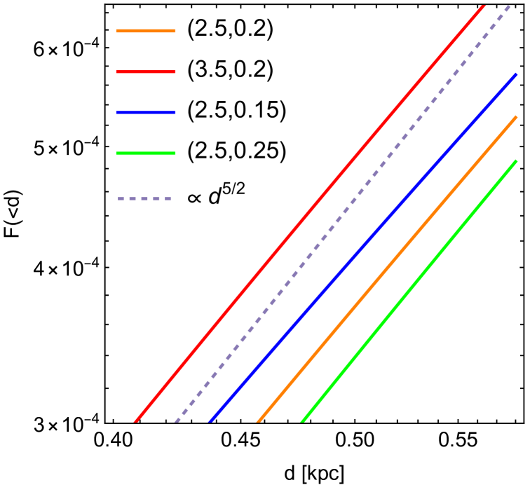
Figure 1: The cumulative fraction $F(<d)$ of Galactic CWDBs within distance $d$ from the Sun. We take four combinations $(R_{D},z_{D})$ for the disk scale lengths. We assume the fraction $C_{D}=2/3$ for the disk component.

Nearby binaries— As discussed earlier, the signal-to-noise ratios $\rho_{3}$ and $\rho_{1}$ are too small for HM Cancri and ZTF J1539 with their reference distances presented in Table I. However, these two binaries are just the tip of the iceberg of the numerous CWDBs to be identified with LISA. Indeed, LISA is expected to detect $N\sim 2000$ detached CWDBs at $f_{2}\gtrsim 4$mHz, completing the whole Galaxy, and a similar number is estimated for AMCVn binaries [11, 7, 13]. There could be undiscovered CWDBs much closer to us (e.g., buried around the directions of the disk plane). We thus evaluate the minimum distance, $d_{\min}$, of Galactic CWDBs at $f_{2}\gtrsim 4$mHz.

For the spatial distribution function of Galactic CWDBs, we use the standard disk model given in the Galactic cylindrical coordinate as

$$F(R,z)=\frac{C_{D}}{4\pi R_{D}^{2}z_{D}}\exp\left({-\frac{R}{R_{D}}-\frac{|z|}{z_{D}}}\right)$$ (16)

with $C_{D}=2/3$ for the fraction of the disk component (ignoring the bulge component around the Sun) and the scaling lengths $(R_{D},z_{D})\sim({\rm 2.5,0.2})$kpc (see, e.g., [11]). By integrating Eq. (16) around the Sun at $(R,z)=(8.3,0)$kpc, we can evaluate the cumulative fraction $F(<d)$ of CWDBs within a given distance $d$ from the Sun. In Fig. 1, we present the numerical results around $d\sim 0.5$kpc for various set of the scaling parameters $(R_{D},z_{D})$. We should obtain $F(<d)\propto d^{3}$ at $d\ll z_{D}$ and $F(<d)\propto d^{2}$ at $z_{D}\ll d\lesssim R_{D}$. Around $d\sim 0.5$kpc, we can approximately have $F(<d)\propto d^{2.5}$.

We can estimate the typical value $d_{\rm c}$ of the minimum distance $d_{\min}$, by solving $N\times F(<d_{\rm c})=1$ and obtain

$$d_{\rm c}\sim 0.5{\rm kpc}\left(\frac{N}{2000}\right)^{0.4}$$ (17)

with a relatively weak dependence on the total number $N$ and the scaling lengths. In reality, the minimum value $d_{\min}$ has statistical fluctuation. Using the fraction $F(<d)$, we can write down a simple differential equation for the probability distribution function of $d_{\rm min}$ and readily obtain the solution

$$P(<d_{\min})=1-\exp\left[-N\cdot F(<d_{\min})\right]$$ (18)

(also from basic expressions for the Poisson distribution). By using Eq. (18) and the scaling relation $F(<d)\propto d^{2.5}$, we evaluate the 80% interval of $d_{\min}$ as $[0.41d_{\rm c},1.4d_{\rm c}]$, with the median value $0.86d_{\rm c}$.

Table 2: Signal to noise ratios of LISA for HM Cancri-like and ZTF J1539-like binaries at $d=0.5$kpc in a 10yr integration.

	$f_{2}$ (mHz)	$d$ (kpc)	$\rho_{2}$	$\rho_{3}$	$\rho_{1}$
HM Cancri-like	6.2	0.5	3340	3.38	1.24
ZTF J1539-like	4.8	0.5	1060	2.28	1.26

In Table II, we present the signal-to-noise ratios $\rho_{i}$ ($i=2,1$ and 3) for the two representative CWDBs now placed at the distance $d=0.5{\rm kpc}\sim d_{c}$ with the extended operation period $T=10$yr proposed for LISA. Note that the maximum value $\rho_{2}\gtrsim 1000$ is generally consistent with previous estimations on CWDBs [30, 31].

The magnitudes $\rho_{3}$ in Table II are close to the detection threshold 5. The distances for $\rho_{3}=5$ are respectively given by 0.338 kpc and 0.228 kpc. Using Eq. (18) and $d_{c}=0.5$ kpc for the two model binaries, the probabilities of having them within the detectable distances become 31% and 13%. Note that we can coherently combine the $f_{3}$ and $f_{1}$ modes. Then the relative accuracy of the scaling parameter $s$ is estimated to be $\delta s/s\sim 1/(\rho_{3}^{2}+\rho_{1}^{2})^{1/2}$.

So far, we have discussed the HH signal search mainly for LISA. Around $f\sim 10$mHz, the design sensitivity $\sqrt{S_{n}(f)}$ of TianQin is close to that of LISA [9], while Taiji is planned to have $\sim 2$ times better sensitivity [8]. Therefore, with their coherent signal integration for 10yr, we can further increase the ratios $\rho_{i}$ by a factor of $\sqrt{1^{2}+1^{2}+2^{2}}\sim 2.5$, indicating the importance of collaborative data analysis. Indeed, after a simple analysis similar to the previous one for LISA alone, we now have the detection probabilities of 98% and 75% respectively for the two model binaries.

Discussions— In this work, we have discussed GWs from circular binaries, including the leading PN correction. However, even at the Newtonian quadrupole order, an eccentric binary emits GWs around multiples of its orbital frequency $f_{\rm o}$. For a small eccentricity $e\ll 1$, the amplitude of the $f_{2}$ mode is given as $A[1+O(e^{2})]$ and those around the frequencies $f_{1}$ and $f_{3}$ are $O(eA)$ [32] with the corresponding signal-to noise ratios $O(e\rho_{2})$. By measuring the amplitude of these two small signals, we can estimate the eccentricity $e$ down to $e=O(1/\rho_{2})$.

Here, one might wonder whether we can distinguish the eccentricity induced Newtonian signal and the PN signal, around the frequency $f_{3}$ (and similarly $f_{1}$). Actually, between the two signals, there is a small frequency gap given by the apsidal precession [e.g., due to the tidal and rotational deformations roughly given by $f_{2}(R/D)^{5}$ as well as the relativistic correction $\sim f_{2}\beta^{2}$] [33, 34, 35]. For an observational period $T\gtrsim 4$ yr, the small frequency gap is likely to be resolved in the matched filtering analysis with the frequency resolution $\sim T^{-1}$ [33, 34, 35], allowing us to differentiate the PN and eccentricity-induced signals around the frequency $f_{3}$.

Meanwhile, some gravitational theories predict the emission of anomalous polarization patterns around the orbital frequency $f=f_{1}$ (e.g., dipole radiations) [36, 37]. These signals could be interesting observational targets for the nearby GW sources and should be cleanly separated from our PN signals at $f=f_{1}$ with the ordinary transverse traceless polarization patterns. Using the strong $f_{2}$ modes of the binaries, we can precisely predict our PN signals, except for the scaling factor $s=\Delta\beta$. Subsequently, by taking an appropriate linear combination of the two TDI data streams (relevant at $f\lesssim f_{*}$), we can effectively cancel the contribution of our PN signals, independent of the factor $s$ (see, e.g., [38]). Then, we can closely examine the anomalous polarization patterns at $f=f_{1}$.

A nearby CWDB would be a golden target also for follow-up EM observations. LISA can localize the sky position of the binary mainly from the Doppler modulation associated with its revolution around the Sun. For an observational period $T\gtrsim 2$yr, the typical area of the error ellipsoid in the sky is estimated to be

$$\delta\Omega=(0.5{\rm arcmin})^{2}\left(\frac{\rho_{2}}{3000}\right)^{-2}\left(\frac{f_{2}}{6.8{\rm mHz}}\right)^{-2}$$ (19)

[39]. Unless the binary is almost at the face-on configuration (where $E_{1}\sim E_{3}\sim 0$), using its GW data, we can predict the expected periodic variations to be searched in EM signals, such as the light curves or the spectral lines [14, 24, 26]. Considering the expected development on the time domain surveys, the binary might be detected even before LISA’s launch.

Once a binary is identified with an EM telescope, we can follow its long-term orbital phase evolution only with EM data (similar to the recent reports on the second derivative ${\ddot{f}}_{\rm o}$ for HM Cancri [22, 23]), reducing the significance of the simple phase analysis on GW data. In contrast, the amplitude measurement (including the HH search) can be done exclusively with GW measurement.

We might determine the distance $d$ to a nearby binary e.g., by an EM parallax measurement. Then, from the GW amplitude $A\propto{\cal M}^{5/3}/d$ of the strong quadrupole mode, we can estimate the chirp mass ${\cal M}$. Additionally measuring the scaling parameter $s=\beta\Delta\propto(m_{a}-m_{b})(m_{a}+m_{b})^{-2/3}$ from the amplitudes of the HH modes, we can, in principle, solve the two masses $m_{a}$ and $m_{b}$ separately.

The long-term future projects such as BBO [40] and DECIGO [41] have been proposed to explore the frequency range 10mHz-10Hz between LISA and ground-based detectors. Around 10mHz, these mid-band detectors have design sensitivities much better than that of LISA and could serve as powerful observatories for further studying the HH signals from Galactic CWDBs.

Summary— We showed that space-based GW detectors, such as LISA, have great potential for detecting the HH modes of GWs for a handful of nearby CWDBs. These overlooked signals are sensitive to the asymmetries of the binaries and would be critically important for complicated systems similar to HM Cancri. The detection prospects can be significantly enhanced through long-term and collaborative operations of the space GW detectors.

Appendix A Intensity functions

Figure 2: The intensity functions $E_{2}$, $E_{1}$ and $E_{3}$ defined in Eqs. (5)(11) and (12).

In Fig. 2, we present the intensity functions $E_{2}(I)$, $E_{3}(I)$ and $E_{1}(I)$ in the range $I\in[0^{\circ},90^{\circ}]$. The functions $E_{2}(I)$ monotonically decreases with $E_{2}(0^{\circ})=2\sqrt{2}$ and $E_{2}(90^{\circ})=1$.

At the face-on configuration $I=0^{\circ}$, we have $E_{1}=E_{3}=0$, reflecting the spin-2 nature of gravitational radiation. They are not monotonic and respectively take the maximum values $E_{1}=(29\sqrt{29/2}-110)^{1/2}=0.65$ at $I=61.2^{\circ}$ and $E_{3}=(15\sqrt{5/2}-21)^{1/2}=1.65$ at $I=48.4^{\circ}$. For reference, we provide the mean squared values $\left\langle E_{2}^{2}\right\rangle_{I}={16}/5,~\left\langle E_{1}^{2}\right\rangle_{I}={5}/{14}$ and $\left\langle E_{3}^{2}\right\rangle_{I}={27}/{14}.$