Towards foundational LiDAR world models
with efficient latent flow matching

Abstract

LiDAR-based world models offer more structured and geometry-aware representations than their image-based counterparts. However, existing LiDAR world models are narrowly trained; each model excels only in the domain for which it was built. Can we develop LiDAR world models that exhibit strong transferability across multiple domains? We conduct the first systematic domain transfer study across three demanding scenarios: (i) outdoor to indoor generalization, (ii) sparse-beam & dense-beam adaptation, and (iii) non-semantic to semantic transfer. Given different amounts of fine-tuning data, our experiments show that a single pre-trained model can achieve up to 11% absolute improvement (83% relative) over training from scratch and outperforms training from scratch in 30/36 of our comparisons. This transferability of dynamic learning significantly reduces the reliance on manually annotated data for semantic occupancy forecasting: our method exceed the previous semantic occupancy forecasting models with only 5% of the labeled training data required by prior models. We also observed inefficiencies of current LiDAR world models, mainly through their under-compression of LiDAR data and inefficient training objectives. To address this, we propose a latent conditional flow matching (CFM)-based frameworks that achieves state-of-the-art reconstruction accuracy using only half the training data and a compression ratio 6 times higher than that of prior methods. Our model achieves SOTA performance on future-trajectory-conditioned semantic occupancy forecasting while being 23x more computationally efficient (a 28x FPS speedup); and achieves SOTA performance on semantic occupancy forecasting while being 2x more computationally efficient (a 1.1x FPS speedup). Project Page: AdaFlowMatchingWM.github.io.

1 Introduction

World models enable agents to implicitly learn the dynamics of the environment by predicting future sensory observations, typically through generative models operating in a latent space rombach2022high ; ma2024latte . Recent advances have led to the development of numerous world models of RGB videos that have demonstrated impressive performance in applications such as autonomous driving russell2025gaia ; hu2023gaia ; wang2024driving , robotic navigation bar2024navigation , and other embodied tasks black2024pi_0 ; kim2024openvlaopensourcevisionlanguageactionmodel ; agarwal2025cosmos ; alhaija2025cosmos . These models can generate video sequences conditioned on historical frames and sometimes natural language input. While an image-based world model may suffice for repetitive tasks (e.g., learning robotic arm movements), its utility may be limited in complex tasks that demand geometrically structured information, such as autonomous driving. In these tasks, the lack of explicit semantic and geometric representations restricts practical applicability, as additional steps are still required to extract explicit spatial information.

In contrast to RGB images, LiDAR provides rich geometric structure and implicitly gives a sparse representation for semantic cues about the environment. Unlike dense, pixel-based observations, a 3D object in a LiDAR point cloud is represented as a cluster of 3D points, encoding essential spatial and semantic information in a compact form. Despite these advantages, foundational world models of LiDAR data remain relatively underexplored: prior LiDAR world models are built for specific domains zhang2023copilot4d ; khurana2023point ; zhang2024bevworld . In comparison, recent advances in “foundation” models, e.g. pretraining with RGB image forecasting alhaija2025cosmos and trajectory forecasting zhou2024smartpretrain have demonstrated the effectiveness of pretraining in improving performance on downstream tasks. Can we develop a foundational LiDAR world model that leads to downstream performance gains on diverse forecasting tasks after fine-tuning? This goal is partly motivated by the fact that many of the causal factors that govern the motion of objects are shared across different domains and environments—many aspects of the dynamics of the world should, in principle, be transferable and can be observed in unlabeled LiDAR.

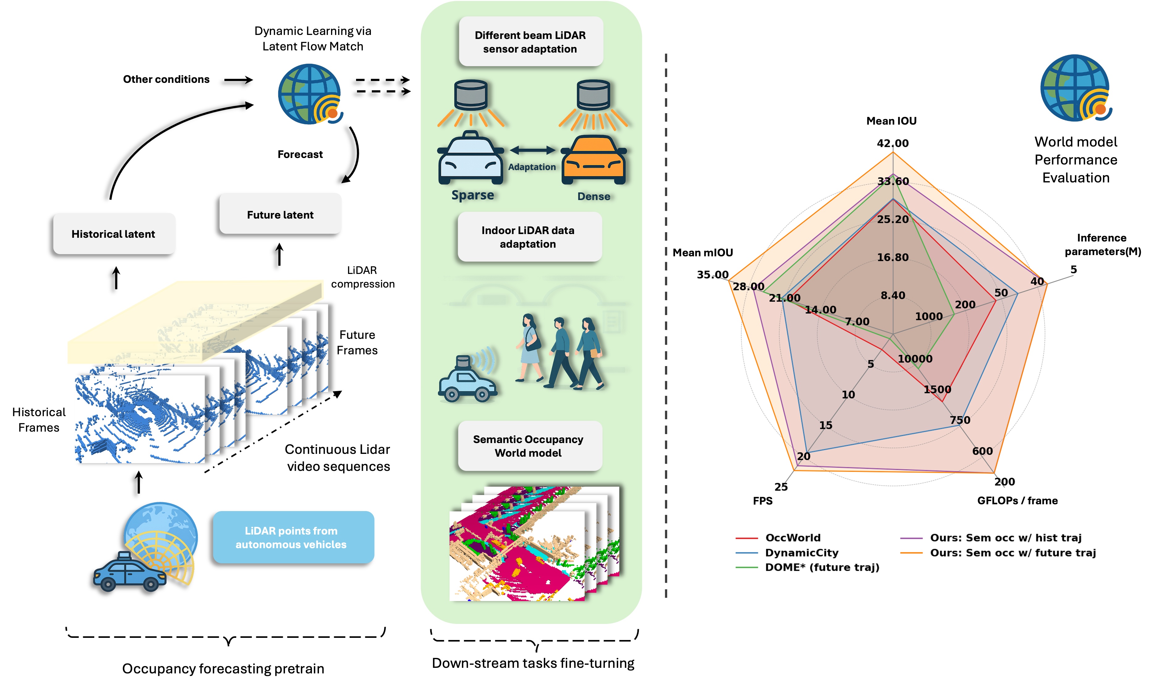
Figure 1: Left: The overall pipeline of our method: we used the most readily publicly available LiDAR dataset from autonomous driving scenarios to train the proposed LiDAR world model. This well-trained world model is able to generalize well on the listed downstream tasks after fine-tuning, although scene and signal properties are quite different. Right: The comparison of our proposed world model with previous methods on nuScenes 4D semantic occupancy forecasting metrics of mIOU, IOU, and inference efficiency. Our approach achieves the best results in terms of both efficiency and performance.

We investigate pretraining and fine-tuning a LiDAR world model across three diverse transfer tasks (Figure 1): varying-beam occupancy forecasting, indoor occupancy forecasting, and semantic occupancy forecasting. First, LiDAR hardware varies in beam count and scan patterns, often degrading model generalization zhang2023copilot4d ; ran2024towards . We consider this cross-sensor setting to assess robustness to hardware variations. Second, robots equipped with LiDAR sensors often operate in vastly different environments wilson2023argoverse ; zhou2021lidar ; han2024dr , from outdoor to indoor settings. While cross-domain adaptation has been extensively studied in perception tasks li2024towards ; michele2024train , it remains underexplored in the context of dynamic learning. Given that the depth range of LiDAR data in certain environments is scarce, it is promising to investigate whether dynamic knowledge learned in data-rich and large-depth-scope domains can be transferred to those with limited data availability and different absolute range. Lastly, for semantic world model tasks (e.g., semantic occupancy forecasting bian2024dynamiccity ; gu2024dome ; li2024uniscene ; zheng2024occworld ) which rely heavily on costly semantic labels wang2023openoccupancy ; tian2023occ3d . Our goal is to leverage large-scale unlabeled data to learn a universal 3D dynamics prior, enabling strong semantic forecasting via fine-tuning on minimal labeled data.

Extensive experiments show that our LiDAR world model can significantly improve the convergence speed of downstream tasks: for all of the mentioned tasks, we observed relative performance gains at different amounts of fine-tuned data. Especially for the task of semantic occupancy forecasting, this scheme of learning environment dynamics before learning semantic patterns allows us to achieve better performance than OccWorld zheng2024occworld with only 5% of the labeled data. Furthermore, we note the importance of representation alignment in the fine-tuning tasks: Although our experiments demonstrate that the data compression structure we propose below is data-efficient, using either the pretrained data compressor directly or retraining the VAE from scratch with the fine-tuned data leads to underwhelming performance. This can be explained by subspace similarity: in both cases, the encoder learns a different feature space mapping from the pretrained one, which hurts the performance of flow models pre-trained on the original feature space. We observe two superior methods: fine-turning the VAE, and separately, applying a cosine-similarity-based alignment loss for tasks on which the original VAE can’t be fine-turned.

We also show current architectural paradigms used in LiDAR world models peebles2023scalable ; esser2024scaling suffer from 2 issues: redundant model parameters and excessive training time. Regarding redundant model parameters: the latent representation tends to retain a large number of channels, which significantly increases dynamic learning model parameter counts. Regarding excessive training time: state-of-the-art models often require thousands of training epochs to converge. This inefficiency stems not only from model scale, but also from the inherently slow and compute-intensive nature of denoising diffusion paradigms—particularly those combining DDPM-based training with DDIM-style sampling.

To address these issues, we propose a Swin Transformer-based VAE architecture for LiDAR data compression, achieving a compression ratio of 192x—over 6x higher than previous state-of-the-art methods—while always maintaining and sometimes exceeding reconstruction quality. We also propose a practical flow-matching-based generative model. Compared to previous latent diffusion-based schemes or transformer-based deterministic schemes, our approach requires only 4.38% and 28.91% of the FLOPs required by them respectively. In summary, our contributions are:

• To the best of our knowledge, this is the first study on building foundational LiDAR world models: world models of LiDAR videos that exhibit substantial transferability to downstream forecasting tasks. We show the efficacy of LiDAR world models to 3 diverse fine-tuning tasks: semantic occupancy forecasting, indoor occupancy forecasting, and high-beams occupancy forecasting, and confirm that it outperforms the baseline of training from scratch on the fine-tuning data, and that the relative performance gains is more pronounced with less fine-tuning data.

• With the decomposed dynamic pretrain + aligned semantic representation fine-tuning approach, we can significantly reduce reliance on human labeled samples for semantic occupancy forecasting: our method can exceed previous methods with only 5% of the semantic data.

• We design efficient architectures for data compression (VAE) and voxel-based LiDAR world modeling. The former achieves the SOTA reconstruction accuracy based on the 6x improvement in compression rate over prior work. Based on such a latent, our dynamic learning model achieves SOTA performance with only 4.47% to 50.23% of the FLOPs and 1.1 to 28.2 times higher FPS.

2 Related Work

We categorize previous work by LiDAR-based world modeling for geometric future prediction, semantic 4D occupancy forecasting for semantic-aware scene understanding, and foundational world models (FWMs) that aim to generalize dynamic knowledge across domains and tasks.

LiDAR-based World Models. Distinct from general LiDAR generation tasks, LiDAR-based world modeling (also known as LiDAR/Occupancy Forecasting) aims to forecast future sensor observations based on past observation. Occ4D khurana2023point and Occ4cast liu2024lidar propose forecasting future LiDAR points or occupancy grids via a differentiable occupancy-to-points module, yet without explicitly modeling latent transition dynamics. UNO agro2024uno further introduces occupancy fields within a NeRF-like mildenhall2021nerf framework to enhance forecast fidelity. S2Net weng2022s2net adopts a pyramid-LSTM architecture to predict future latents extracted by a variational RNN, while PCPNet luo2023pcpnet leverages range-view semantic maps and a transformer backbone to improve real-time inference performance. Although numerous works nunes2024scaling ; ran2024towards ; xiong2023ultralidar ; nakashima2024fast ; karras2022elucidating have introduced increasingly powerful diffusion-based models, for general data generation, progress in LiDAR forecasting remains comparatively limited compare to the RGB-base ones: Copilot4D zhang2023copilot4d achieved state-of-the-art performance in LiDAR forecasting by adopting a MaskGiT-based latent diffusion model with a carefully-designed temporal modeling objective. BEVWorld zhang2024bevworld extended this approach by incorporating multi-modal sensor inputs, enabling future LiDAR prediction even in the absence of current LiDAR frames. However, few works have addressed the transferability of dynamics learning across domains—an appealing path to enhance the widespread deployment of world models in real-world autonomous systems.

Semantic 4D Occupancy Forecasting: The RGB video based world models tried to forecast physical consistent video from RGB input. However, these representations lack of geometric and explicit semantic annotation, the usage of the generated forecasts observations in control task still need extra component to recover depth and predict semantics. Semantic 4D occupancy forecasting aims to address this gap by predicting future semantic (LiDAR) occupancy maps based on past observations—either ground-truth annotations or model-generated results. OccWorld zheng2024occworld employed an auto-regressive transformer to jointly forecast future latent states and corresponding axis offsets. OccSora wang2024occsora further advanced the field by being the first to generate 25 seconds semantic videos conditioned on 512x compressed inputs. Later, DynamicCity bian2024dynamiccity improved upon this by decomposing the 3D representation into a more compact HexPlanecao2023hexplane structure, enabling faster inference. Building upon future trajectories/bev layout and extended datasets, DOME gu2024dome and uniScenes li2024uniscene continue to push the forecasting accuracy to new state-of-the-art levels. Importantly, these methods rely on labeled semantic ground-truth data for training, making them dependent on expensive human annotations and thus challenging to scale.

Foundational world model (FWM). We call a world model “foundational” if it leads to performance gains over learning from scratch on multiple downstream forecasting tasks. In autonomous driving, GAIA-1 hu2023gaia and GAIA-2 russell2025gaia introduced image-based FWMs that can generate controllable driving scenarios. In the field of indoor robotics, like navigation, NWM bar2024navigation proposed an RGB image-based navigation method with a conditional DiT structure. Cosmos agarwal2025cosmos takes this ambition further, aiming to generalize across both indoor and outdoor environments. However, due to limitations in the RGB modality, existing FWMs do not provide explicit depth information, which makes it harder to define prediction and planning modules to utilize their output.

3 Efficient latent conditional flow matching

In this section, we first introduce our novel point cloud data compressor in Sec.3.1, which achieves state-of-the-art performance under high compression ratio. Based on the compact representation from it, Sec.3.2 presents the flow matching-based generative forecasting model that serves as the testbed for all subsequent fine-tuning approaches. In Sec.3.3, we introduce the VAE fine-tuning for better representation alignment, which will benefit the final forecast performance.

3.1 Data compression

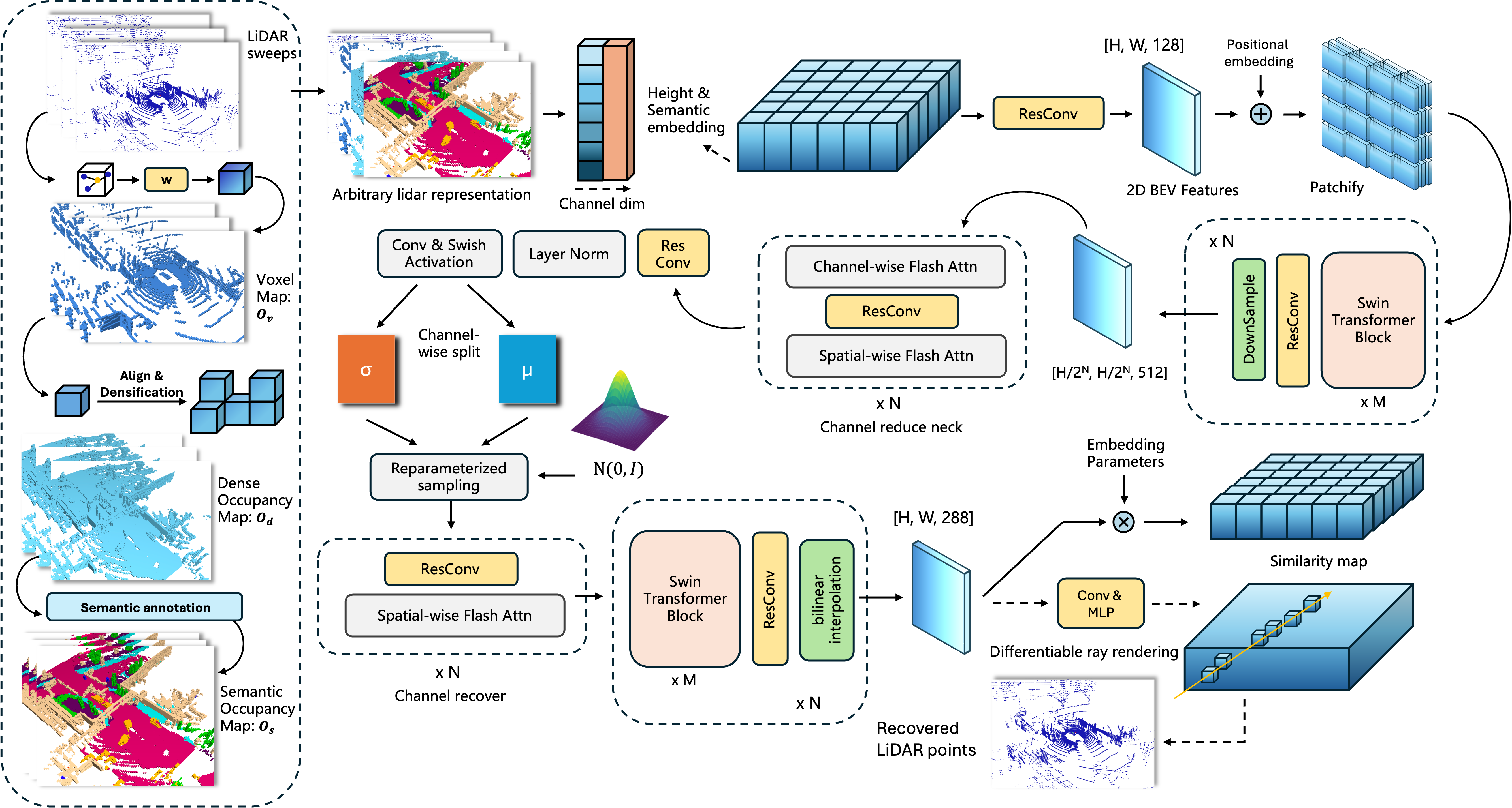
Figure 2: Architecture of our VAE for LiDAR compression. The model enables high compression ratios—exceeding those of previous methods—alongside high-fidelity reconstructions.

For compressing image-based RGB signals, SD3 esser2024scaling provides a strong baseline. However, LiDAR-specific data compression remains underexplored. Existing LiDAR world models typically adopt SD3’s encoder-decoder architecture with minimal modifications, retraining it directly on LiDAR BEV representations. Based on the Swin Transformer, we propose a new option and find it has the leading performance on all forms of LiDAR compression in Table 2. As noted in previous works li2024uniscene , discrete coding-based compression is not only prone to problems such as codebook collapse, but is also generally inefficient in compression. Here we have also used continuous coding to achieve a higher compression ratio as shown in Fig. 2.

Data processing and encoding: Hereafter, bolding indicates a multidimensional array (e.g., a vector or a matrix). Given a raw LiDAR sensor scan $\bm{o}_{l}\in\mathbb{R}^{L\times 3}$, the voxelized map $\bm{o}_{v}$, dense occupancy map $\bm{o}_{d}$, and semantic occupancy map $\bm{o}_{s}$ can be generated through successive steps of voxelization, densification (using the entire LiDAR sequence to include points to each frame), and semantic annotation. Our structure is capable of processing any of these representations derived from the raw LiDAR input. Depending on the final reconstruction requirements, voxelization can be either a learning-based approach or a direct binarization process. Taking the compression of $\bm{o}_{d}\in\mathbb{R}^{H\times W\times D\times C}$(a $H,W,D$ 3D grid with C-dim features at each voxel) as an example, a Gaussian encoding distribution $q(\bm{z}_{d}|\bm{o}_{d})\!=\!\mathcal{N}(\bm{z}_{d};\bm{\mu}_{q},\bm{\sigma}_{q})$ is constructed from three main stages: embedding, feature learning and downsampling, and channel reduction. Specifically, after applying height and class embeddings, a 2D BEV feature map is obtained, which is subsequently processed by a standard 2D Swin Transformer encoder. Unlike the original Swin Transformer design, which utilizes patch merging for downsampling, we replace it with conventional convolutional layers, which will later be shown to outperform the former approach. Channel reduction is performed by a lightweight network neck, compressing the feature representation into a 16-dimensional latent space. Samples are drawn using the reparameterization trick $\bm{z}\!=\!\bm{\mu}_{q}+\bm{\sigma}_{q}\odot\bm{\epsilon}$, $\bm{\epsilon}\sim\mathcal{N}(0,\bm{I})$, and $\odot$ is the Hadamard product.

Decoding and $\bm{o}_{l}$ representation recovery. The decoder $q(\hat{\bm{o}}_{d}\mid\bm{z}_{d})$ is designed to mirror the encoder by starting with the same symmetric 2D block structure. Different from the previous method that used 3D blocks in the decoder to increase temporal feature consistency, we found that it’s actually have a negative effect in our structure, for both reconstruction and final forecasting result, as shown in the ablation study. Depending on the source representation, the reconstructed $\hat{\bm{o}}_{d}$ can be used to render the points with a differentiable ray rendering module or get the occupancy map by calculating a similarity score with the class embedding.

3.2 Forecasting with Conditional flow matching

With the VAE proposed, we are able to mitigate the parameter redundancy: most of the parameters of the existing methods come from the high dimensionality of the latents. To further make the training of the model more efficient, we present a new structure based on flow matching, which we show leads to SOTA performance in both forecasting accuracy and calculation efficiency as shown in Table 1. For a semantic occupancy forecast task, given $\bm{o}_{s}^{t_{0}:t_{2}}$, our VAE will compress these continuous frames to $\bm{z}_{s}^{t_{0}:t_{2}}\in\mathbb{R}^{(t_{2}-t_{0})\times H\times W\times 16}$. Given the $t_{1}$ is the middle index of these frames, our objective is to obtain the future latent $\bm{z}_{s}^{t_{1}:t_{2}}$ from the historical latent $\bm{z}_{s}^{t_{0}:t_{1}}$ using a flow-matching model $G_{\theta}$.

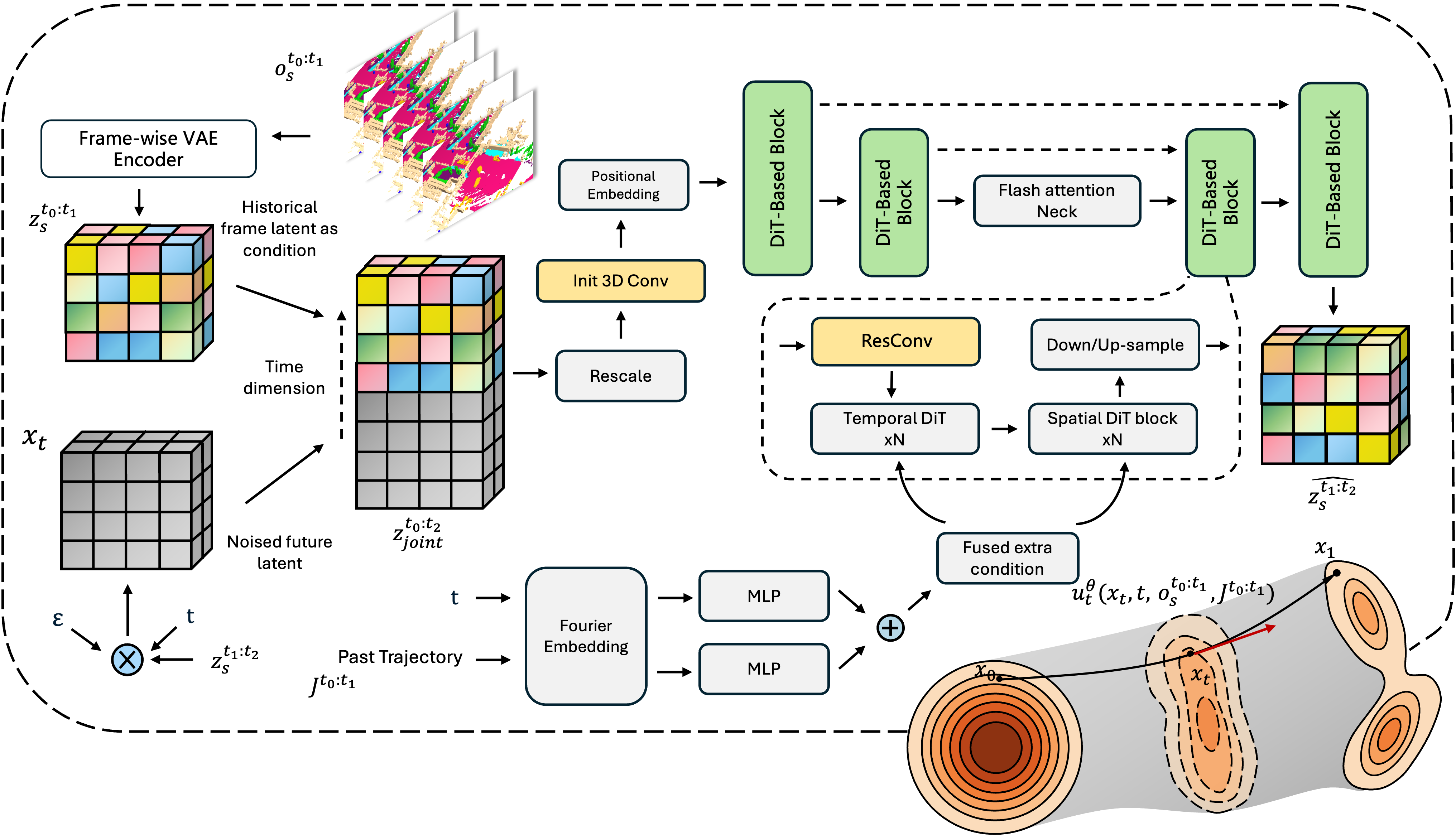
Figure 3: Architecture of our conditional velocity field predictor at time $t$. Historical frame latents are extracted via a frame-wise VAE encoder, and noised future latents are formed by injecting noise at timestep $t$. Latents are concatenated along the time dimension and passed through DiT blocks.

As shown in Figure 4, during the training stage, given a time point $t\in[0,1]$ represents the progress along the probability path from initial distribution(Standard Gaussian) to target distribution, the noised future latent $x_{t}$, the historical trajectory $J^{t_{0}:t_{1}}\in\mathbb{R}^{(t_{1}-t_{0})\times 3}$, and historical observation $\bm{o}_{s}^{t_{0}:t_{1}}$, the velocity field $u_{t}^{\theta}$ is regressed. Specifically, the noising added follows a linear interpolation method as shown in the equation 1, where $\sigma$ used to balance the scale of noise and latents and $\epsilon\sim\mathcal{N}(0,1)$. The $\bm{z}_{s}^{t_{0}:t_{1}}$ will be used as a part of condition in training: we concatenate the historical latents and noised future latents along time dimension to get the input of ${G}_{\theta}$, denoted by $\mathbf{z}_{\text{joint}}\in\mathbb{R}^{(t_{2}-t_{0})\times H\times W\times 32}$.

$$\mathbf{x}_{t}=(1-t)\bm{\epsilon}+t\sigma\bm{z}_{s}^{t_{1}:t_{2}}$$ (1)

Based on the spatial-temporal DiT structure proposed in previous methods ma2024latte ; li2024uniscene ; gu2024dome , we observe that the convergence speed remains suboptimal. Specifically, given $\mathbf{z}_{\text{joint}}$, the initial 3D convolutional layer increases the channel dimension to $C^{\prime}$, resulting in $\mathbf{z}^{\prime}_{\text{joint}}\in\mathbb{R}^{(t_{2}-t_{0})\times H\times W\times C^{\prime}}$. The width and height dimensions are then flattened before being fed into the spatial DiT, where multi-head attention (MHA) is applied and normalized using AdaLN. However, applying the same strategy in the temporal DiT would only fuse pixels along the temporal axis, limiting the temporal receptive field to just a single latent pixel(in a block). Therefore, we observed that most of the previous method like uniScenes li2024uniscene and DOME gu2024dome use 14-18 stacked blocks to ensure the temporal consistency, which is also one of the reasons of redundant parameters. While this design remains feasible in Latte ma2024latte , which operates on 3D video patches, our setting involves individual latents containing only one frame of information, making the learning of temporal dependencies more challenging. Fortunately, this issue can be effectively mitigated by simply adding a 3D convolutional layer with a larger receptive field after the spatial DiT. Furthermore, organizing the network in a UNet-style architecture, as opposed to a single-stride DiT backbone, is shown through later experiments to further enhance the forecast performance.

The overall training objective was design following the Rectified Flow liu2022flow :

$$\mathcal{L}(\theta)=\mathbb{E}_{t,\bm{x}_{0},\bm{z}_{s},J}\left\|\mu_{t}^{\theta}(\bm{z})-(\bm{z}_{s}-\bm{x}_{0})\right\|^{2},\quad t\sim\texttt{sigmoid}(\mathcal{N}(0,1)),\;\bm{x}_{0}\sim\mathcal{N}(\bm{0},\bm{I}),\;\bm{z}_{s}\sim q_{\bm{z}_{s}}.$$

3.3 Improved fine-tuning with representation alignment

To fine-tune the foundational model, we need to feed the data compressor the LiDAR representation from potentially very different domains. We found it important to “align“ the representations of the pre-trained and fine-tuned data prior to use latter to fine-tune the flow matching model. However, in case of subtask 3 (semantic occupancy forecasting), due to the difference in network embedding layer dimensions, it is non-trivial to fine-tune the semantic data based on a VAE pretrained on non-semantic data. Instead, we use the latents of the corresponding dense occupancy $\bm{o}_{d}$ to guide the formulation of the subspace of the semantic VAE.

Specifically, we add a cosine similarity term in the loss when fine-tuning the VAE, as shown in the last term of Equation 2. $\bm{z}_{s}$ and $d_{s}$ stand for the latent from a pair $\bm{o}_{s}$ and $\bm{o}_{d}$ via training from scratch and pretrained VAE, respectively. $\mathcal{L}_{\text{lovasz}}$ berman2018lovasz is another reconstruction term used to optimize IOU.

$$\mathcal{L}_{\text{Sem-VAE}}=\mathcal{L}_{\text{CE}}(\hat{\bm{o}}_{s},\bm{o}_{s})+\beta D_{\text{KL}}\left(q_{\phi}(\mathbf{z_{s}}\mid\mathbf{o_{s}})\,\|\,p(\mathbf{z_{s}})\right)+\lambda\mathcal{L}_{\text{lovasz}}(\hat{\bm{o}}_{s},\bm{o}_{s})+\kappa\mathcal{L}_{\text{cos}}(\bm{z}_{s},\bm{d}_{s})$$ (2)

4 Experiments

We designed our experiments to investigate the following questions: Q1: Can we improve compression and model performance over existing designs? Q2: Can we develop a LiDAR world model that exhibits substantial superiority to models trained from scratch on three downstream forecasting tasks (high-beams occupancy forecasting, indoor occupancy forecasting, and semantic occupancy forecasting)? Q3: How well does each fine-tuning variant perform and why does fine-tuning the representation work?

4.1 Experimental design

We use nuScenes (2Hz) as the pre-training data for the flow matching model. We trained 2 different types of foundational models on it, one was trained based on the original lidar sweep ($\bm{o}_{v}$), totaling 27,000 frames, denoted by ${G}_{\theta}^{v}$. The other one was trained based on LiDAR frames after they have been densified ($\bm{o}_{d}$), totaling 19,000 frames, denoted by ${G}_{\theta}^{d}$. The latter training set is a subset of the former part and the number of $\bm{o}_{d}$ equal to $\bm{o}_{s}$.

For the different beam adaptation subtask, we downsampled 11 sequences from the KITTI360 raw dataset liao2022kitti from 10Hz to 2Hz to match the foundational model setting. Also, we collected an indoor navigation dataset using a Clearpath Jackal equipped with an OSO-128 LiDAR sensor (training set with 23,504 frames and validation set with 9,720 frames). Finally, for the semantic occupancy forecasting, we present a 2 fold experiments: in section 4.2, we follow the official splitting tian2023occ3d and train the model from scratch. Then in section and H.1, we only use first half of the training data to pretrain the $G_{\theta}^{d}$ as the foundation model, which then fine-tuning on the other half $\bm{o}_{s}$ ($\bm{o}_{s}$ and $\bm{o}_{d}$ are 1v1 correspondence) to avoid fine-tuning data to be already seen during pretraining stage. From the next section, we use $\bm{o}_{s}^{\prime}$ and $\bm{o}_{d}^{\prime}$ to denote the partial training data. For more details on the model setup, please refer to our appendix.

4.2 Encoder structure exploration and semantic occupancy forecasting evaluation

For model evaluation, Table 2 compare reconstruction results of our Swin-Transformer VAE with previous methods compress data from 8× to 512×. At 32×, we achieve 99.2% mIoU and 97.9% IoU—far above UniScenes’s 92.1%/87.0% at the same rate. Even at 192×, we maintain 93.9%/85.8%, surpassing OccWorld and DOME by over 11% mIoU, and at an extreme 768× our model still delivers a 9.7% relative gain despite 1.5× higher compression.

Table 1: Comparison of future occupancy forecasting performance on full nuS. validation set. $\dagger$ Methods use future trajectory information. $\star$ DynamicCity generates 16 frames jointly; …

Method	mIoU$\uparrow$				IoU$\uparrow$				Mean NLL (bits/dim)$\uparrow$	Mean FID$\downarrow$	GFLOPs per Frame$\downarrow$	FPS$\uparrow$
	1s	2s	3s	Avg	1s	2s	3s	Avg
OccWorld zheng2024occworld	25.75	15.14	10.51	17.13	34.63	25.07	20.19	26.63	–	8.62	1347.09	2.56
RenderWorld yan2024renderworld	28.69	18.89	14.83	20.80	37.74	28.41	24.08	30.08	–	–	–	–
OccLLama wei2024occllama	25.05	19.49	15.26	19.93	34.56	25.83	24.41	29.17	–	–	–	–
DynamicCity⋆ bian2024dynamiccity	26.18	16.94	–	–	34.12	25.82	–	–	–	–	774.44	19.30
gray!10 Ours	33.17	21.09	15.64	23.33	40.53	30.37	24.44	31.78	6.29	2.83	389.46	22.22
DOME† gu2024dome	29.39	20.98	16.17	22.18	38.84	31.25	26.30	32.13	6.04	5.03	8891.98	0.76
gray!10 Ours†	36.42	27.39	21.66	28.49	43.68	36.89	31.98	37.52	4.55	2.80	389.46	21.43

Table 2: Occupancy reconstruction performance comparison at various compression ratios.

Method	Cont.?	Comp. Ratio$\uparrow$	mIoU$\uparrow$	IoU$\uparrow$
OccLlama wei2024occllama	✗	8	75.2	63.8
OccWorld zheng2024occworld	✗	16	65.7	62.2
OccSora wang2024occsora	✗	512	27.4	37.0
DOME gu2024dome	✓	64	83.1	77.3
UniScenes li2024uniscene	✓	32	92.1	87.0
UniScenes li2024uniscene	✓	512	72.9	64.1
gray!10 Ours	✓	32	99.2	97.9
gray!10 Ours	✓	192	93.8	85.8
gray!10 Ours	✓	384	88.3	76.9
gray!10 Ours	✓	768	80.0	69.3

Based on the strong VAE performance, our forecasting model advances the state-of-the-art in semantic occupancy forecasting task and preserves a compact footprint and real time throughput. As shown in Table 1, our model achieves a one-second mIoU of 33.17%, surpassing the previous SOTA model’s 28.69% and OccLLama’s 25.05% by 4.48% and 8.12% respectively and maintaining 21.09% and 15.64% for two and three second prediction which outpaces prior works by at least 2.5% relative performance improvement. Considerable margin is also conveyed in terms of IoU, in average 1.70% higher than previous SOTA model. For future-trajectory-conditioned forecasting, our mIoU surpasses DOME by more than 5.5% across all frames. Critically, these predictive gains from our proposed VAE plus CFM network incur almost no computational overhead. Our semantic occupancy forecasting model runs at 22.22 FPS, requiring only 389.46 GFlops per frame and 30.37 million parameters. Compared to OccWorld, our model achieves around 6% of absolute performance improvement while using only 28.91% of computational cost, less than 50% of the parameters, and almost 10 times faster inference speed. Even for DynamicCity which generates 16 frames altogether, our model uses half of GFlops per frame, 66% of parameters, and 1.1 times higher FPS. In the future-trajectory-conditioned regime, our model sustains 21.4 FPS without increasing in computational cost and parameter count, whereas DOME utilizes 23 times more flops per frame (our model is 4.38% of this amount), 15 times more parameters, 28 times slower FPS, and at least 5.5% less absolute performance. Other metrics: In order to evaluate generative quality of our proposed framework, we report the 3D Fréchet Inception Distance (FID) in Table 1. Moreover, due to the stochastic nature of our proposed CFM model and the limitation of mIoU and IoU in evaluating model’s ability to generate diverse but plausible future predictions, we report the negative log likelihood (NLL) in bits-per-dimension. Please refer to Appendix for more details on parameter counts, metrics computation and performance analysis.

4.3 LiDAR world model transferability

Using the architecture in Section 4.2 and outdoor-pretrained weights, we evaluate the performance gains from fine-tuning our foundational world model with varying strategies and data scales across individual tasks and present the results in Fig.4. For the high-beam LiDAR adaptation task, all configurations based on the pretrained world model outperform from-scratch VAE and CFM training (blue line) across all frames and data fractions. Pretraining CFM alone yields 17.11% and 6.68% gains for 1s and 3s predictions at 10% data. With both components pretrained and fine-tuned, the gains increase to 14.48% and 26%, respectively. This demonstrates that our Swin Transformer-based VAE effectively captures transferable geometric priors for downstream tasks with varying LiDAR characteristics and the effectiveness of the feature alignment.

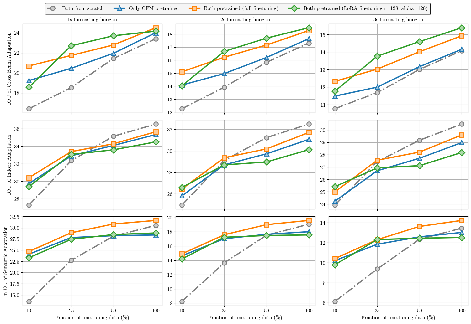
Figure 4: IoU/mIoU comparison across 3s forecasting horizon of the presence of different fraction of fine-tuning data used from total data available between the various training procedures. In row order, each row refers to the results of (i) different beam adaptation (ii) outdoor-indoor adaptation, and (iii) semantic occupancy forecasting, respectively.

For the indoor LiDAR adaptation task, all pretrained model variants outperform from-scratch training when fine-tuning data is limited (less than 25%), with full-parameter tuning of both VAE and CFM achieving the best results. At 10% data usage, full fine-tuning yields at least a 4.47% gain across all prediction horizons. However, as data availability increases (e.g., beyond 25% for 1s prediction), from-scratch training surpasses all fine-tuning methods. This is likely because the indoor dataset is a more distinct task relative to the other tasks, making it easier to learn from scratch without pretrained dynamic priors. We expect this result would no longer hold if substantial indoor data was in the pretraining data. See Appendix for further explanation.

We can also observe similar results in semantic occupancy forecasting task, all VAE/CFM combinations based on the pretrained model outperform training from scratch in mIoU. Notably, at 10% semantic fine-tuning data—which is only 5% of the total used in prior methods—full-parameter fine-tuning yields an 82.6%/80.72%/69.70% relative mIoU gain for 1s/2s/3s prediction, which surpasses OccWorld’s performance zheng2024occworld . After 50% data usage, the performance of from-scratch, exceed that of pretrain CFM-only, and LoRA CFM fine-tuning, while full-parameter VAE+CFM fine-tuning consistently achieves the best performance across all data fractions and prediction horizons.

These results confirm that foundational models can capture transferable LiDAR-based dynamic priors from unlabeled data, supporting downstream tasks requiring semantic interpretation. The improvements are especially notable under low-data regimes, demonstrating reduced dependence on human-labeled samples. Overall, across all tasks, our pretrained model achieves up to 11.17% absolute performance gain, and outperforms training from scratch in 30/36 comparisons points. See Appendix for detailed numerical values corresponding to Figure 4.

However, one question remaining is that why models that have both VAE and CFM modules pretrained (with or without LoRA) consistently possesses higher absolute performance over other settings? In other words, how does fine-turning VAE impact CFM forecasting accuracy?

To further analyse, in Table 3, we compute the similarity of latent spaces under different data scales using CKA kornblith2019similarityneuralnetworkrepresentations and CKNNA huh2024platonic . The similarities are measured between pairwise samples w/w.o semantic information, i.e., $\bm{o}_{d}^{\prime}$ with $\bm{o}_{s}^{\prime}$ obtained from finetuned VAE or VAE trained only on fine-turning data. We observe that the effectiveness of VAE fine-tuning is primarily attributed to aligning the latent space of the new domain with that of the original domain, rather than improving reconstruction accuracy. For example, when using 100% of the fine-turning data $\bm{o}_{s}^{\prime}$, the non-pretrained VAE achieves even higher mIoU/IoU than the pretrained one, yet the final performance shows a clear gap—suggesting that preserving latent structure plays a more crucial role. Although paired data is not available for the first two adaptation scenarios, estimating latent similarity in other domains could further support our hypothesis, details are shown in Appendix.

4.4 Ablation study

Table 3: VAE fine-tuning evaluation in non-semantic to semantic adaptation.

Pretrain	Fine-tuning	mIoU	IoU	CKA	CKNNA	Cosine
$\bm{o}_{d}^{\prime}$	10% $\bm{o}_{s}^{\prime}$	87.97	75.22	0.739	0.278	0.907
$\varnothing$	10% $\bm{o}_{s}^{\prime}$	75.81	72.27	0.653	0.221	0.183
$\bm{o}_{d}^{\prime}$	25% $\bm{o}_{s}^{\prime}$	88.91	76.92	0.721	0.273	0.900
$\varnothing$	25% $\bm{o}_{s}^{\prime}$	83.09	75.92	0.619	0.205	0.226
$\bm{o}_{d}^{\prime}$	50% $\bm{o}_{s}^{\prime}$	89.72	80.09	0.744	0.275	0.901
$\varnothing$	50% $\bm{o}_{s}^{\prime}$	90.26	82.03	0.600	0.194	0.237
$\bm{o}_{d}^{\prime}$	100% $\bm{o}_{s}^{\prime}$	92.10	82.56	0.750	0.275	0.910
$\varnothing$	100% $\bm{o}_{s}^{\prime}$	92.14	83.41	0.628	0.199	0.219

Table 4: Ablation study of different designs in dynamic learning. We use 3s Mean mIOU here, all experiments trained for 100 epochs.

Method	U-Net	CFM	3D Conv after Temporal DiT	CFG	Scale	mIOU
+ Baseline	✗	✗	✗	✗	1.0	17.42
+ UNet	✓	✗	✗	✗	1.0	17.77
+ CFM	✓	✓	✗	✗	1.0	20.14
+ 3D Conv	✓	✓	✓	✗	1.0	20.67
+ CFG	✓	✓	✓	✓	1.0	21.05
+ Rescale	✓	✓	✓	✓	10	23.33

As mentioned in Section 3.2, we now present a breakdown of the performance improvements contributed by each individual module. As shown in Table 4, we observe consistent gains from CFM, 3D convolution, and CFG components, while using classifier free guidance give us the most significant improvement in both IoU and mIoU. We also experiment the impact of the choice of NFE on FLOPS, FPS, and accuracy. In taking NFE=10, we get the best forecasting accuracy while maitaining considerable level of efficiency in terms of run time and GFlops for semantic occupancy forecasting task. For experiment of VAE data-efficient and other details, please see the Appendix.

5 Conclusion

In this work, by designing a model that can be efficiently pretrained on large-scale outdoor LiDAR data, we show it can be effectively fine-tuned on diverse downstream tasks. Our approach consistently outperforms training from scratch, especially in low-data regimes. To address inefficiencies in existing models, we introduce a new VAE stucture for high-ratio LiDAR compression and a conditional flow matching approach for forecasting. These components enable strong reconstruction performance and improve training and inference efficiency without sacrificing forecasting accuracy. In addition, our VAE fine-tuning strategies further boost performance. While results are encouraging, future work is needed to extend generalization to additional environments, incorporate multi-modal inputs, and integrate with planning and control systems. Overall, our findings suggest that scalable and transferable LiDAR world models are feasible and can significantly reduce reliance on annotated data in practical applications.

Appendix

Contents

1. 1 Introduction
2. 2 Related Work
3. 3 Efficient latent conditional flow matching
   1. 3.1 Data compression
   2. 3.2 Forecasting with Conditional flow matching
   3. 3.3 Improved fine-tuning with representation alignment
4. 4 Experiments
   1. 4.1 Experimental design
   2. 4.2 Encoder structure exploration and semantic occupancy forecasting evaluation
   3. 4.3 LiDAR world model transferability
   4. 4.4 Ablation study
5. 5 Conclusion
6. A Model Setup and Further Evaluation
   1. A.1 Training Setup
   2. A.2 Latent space similarity metrics
   3. A.3 Inception-based metrics
   4. A.4 Negative log likelihood evaluation
      1. A.4.1 Computation of exact log probability density
      2. A.4.2 Details on NLL evaluation
      3. A.4.3 DDPM log likelihood computation
      4. A.4.4 Results on semantic occupancy forecasting task
7. B Dataset introduction
8. C Detailed pretraining and fine-tuning results
   1. C.1 High-beam adaptation and indoor occupancy forecasting
   2. C.2 Semantic Occupancy Forecasting
9. D More details on representation alignment
10. E Analysis on LoRA fine-tuning with different ranks
11. F Additional ablation studies
    1. F.1 The data efficiency of proposed VAE structure
    2. F.2 Results of forecasting on pretraining data
    3. F.3 VAE and forecasting result break down
    4. F.4 NFE selection for CFM solver during inference
    5. F.5 Model performance with different fractions of pretraining data
    6. F.6 CFM performance sensitivity analysis with sampling randomization
12. G Limitation and future work
13. H Visualization
    1. H.1 Samples from the pretrained model
    2. H.2 Samples from the semantic occupancy forecasting model

Appendix A Model Setup and Further Evaluation

A.1 Training Setup

For all flow matching based generative (foundational) model training, different from previous methods gu2024dome ; li2024uniscene that used several thousands of training epochs, we used 4x RTX 4090 to train models for 200 epochs with batch size 8. We trained the VAE part for 100 epochs with batch size 16 if not specified.

Following prior workzhang2023copilot4d , we also adopt the AdamW as the optimizer with $\beta_{1}$ and $\beta_{2}$ set to 0.9 and 0.99 for Flow matching training, 0.99 and 0.999 for VAE training. We set the weight decay of all normalization layers to 0 and all of other layers’ to 0.001. The learning rate schedule has a linear warmup followed by cosine decay (with the minimum of the cosine decay set to be 20% of the peak learning rate). We also use EMA with 0.9999 decay rate to ensure the updates of parameters are stable. During the training, we found that the conditional free guidance is also important in a flow-matching based framework. We randomly set 25% of historical latent in a batch to 0 during training to let model learn to generate future latents without any condition. In the sampling phase, we use a typical fuse method as shown in Eq. 3 to get the final output when it’s the $t$-th step, where s set to 2.

$$\hat{\mu}_{\theta}(\bm{z}_{t},t,c;s)\;=\;(1+s)\,\bm{\mu}_{\theta}(\bm{z}_{t},t,c)\;-\;s\,\bm{\mu}_{\theta}(\bm{z}_{t},t,\varnothing)$$ (3)

Finally, we also noticed that the matching of noise scale and latent scale is important. Different from SD3’s VAE, the value of latent obtained from our VAE is actually smaller, with a standard deviation of about 0.02, which makes it easy to drown the signal in noise if we use standard Gaussian noise if we use it in the training phase. Therefore, we scaled the compressed latent by a factor of 10 in the implementation.

A.2 Latent space similarity metrics

Given $\bm{o}_{d}\in\mathbb{R}^{H\times W\times D\times C}$ and its compressed latent $\bm{z}\in\mathbb{R}^{h\times w\times c}$, the compression ratio $\gamma$ can be calculated as in Eq. 4.

$$\gamma=\frac{h\times w\times c}{H\times W\times D\times C}$$ (4)

In Section 4.3, we introduce CKA(Centered Kernel Alignment) kornblith2019similarityneuralnetworkrepresentations and CKNNA(Centered Kernel Nearest-Neighbor Alignment )huh2024platonic to evaluate the similarity of latent space, both of them are insensitive to linear transformations. Specifically, we treat each latent pixel (location) as an individual sample i.e., every sample in CKA/CKNNA evaluation can be represented as $\bm{z}_{i}\in\mathbb{R}^{1\times c}$. For non-semantic to semantic adaptation subtask, given $\mathbf{k}$ samples from $\mathbf{e}$ latent, the representation metrics from $\bm{o}_{d}$ and $\bm{o}_{s}$ can be denoted by $\bm{X}\in\mathbb{R}^{u\times c}$ and $\bm{Y}\in\mathbb{R}^{u\times c}$ respectively. We first construct kernel matrix:

$$\bm{K}_{ij}=\exp\left(-\frac{\|\bm{X}_{i}-\bm{X}_{j}\|^{2}}{2\sigma^{2}}\right),\quad\bm{L}_{ij}=\exp\left(-\frac{\|\bm{Y}_{i}-\bm{Y}_{j}\|^{2}}{2\sigma^{2}}\right)$$ (5)

Then the CKA can be calculated as:

$$\mathrm{CKA}_{\text{RBF}}(\bm{X},\bm{Y})=\frac{\mathrm{tr}(\bm{K}_{c}\bm{L}_{c})}{\sqrt{\mathrm{tr}(\bm{K}_{c}\bm{K}_{c})\cdot\mathrm{tr}(\bm{L}_{c}\bm{L}_{c})}}$$ (6)

where $\bm{K}_{c}$ and $\bm{L}_{c}$ are centered $\bm{K}$ and $\bm{L}$, using $\bm{K}_{c}=HKH$, $H=I_{n}-\frac{1}{n}\bm{1}_{n}\bm{1}_{n}^{T}$. $\bm{1}_{n}$ is all-ones column vector. CKNNA is a revised version of CKA which focus on the local manifold similarity.

For every sample $i$ in $K_{c}$ and $L_{c}$, we use cosine similarity to find out the nearest k neighbor in original samples, let $\mathrm{knn}_{K_{c}}$ and $\mathrm{knn}_{L_{c}}$ be the indices of its k nearest neighbors, respectively. Then we can define a mutual-KNN mask $\alpha(i,j)$ by:

$$\alpha_{ij}\;=\;\begin{cases}1,&j\in\mathrm{knn}_{K_{c}}(i)\ \wedge\ j\in\mathrm{knn}_{L_{c}}(i),\\[4.0pt] 0,&\text{otherwise},\end{cases}\qquad i\neq j.$$ (7)

Local alignment is $\text{Align}_{KNN}(\bm{K}_{c},\bm{L}_{c})=\sum_{i=1}^{u}\sum_{j=1}^{u}\alpha(i,j)\,\bm{K}_{c}(i,j)\,\bm{L}_{c}(i,j)$. CKNNA is:

$$\operatorname{CKNNA}(\mathbf{K},\mathbf{L})\;=\;\frac{\operatorname{Align}_{k\text{nn}}\!\bigl{(}\bm{K_{c}},\bm{L_{c}}\bigr{)}}{\sqrt{\operatorname{Align}_{k\text{nn}}\!\bigl{(}\bm{K_{c}},\bm{K_{c}}\bigr{)}\;\operatorname{Align}_{k\text{nn}}\!\bigl{(}\bm{L_{c}},\bm{L_{c}}\bigr{)}}}$$ (8)

Use k to represent the number of neighbors we selected, when $k\!\to\!u,\alpha_{ij}=1$ for all off-diagonal pairs and CKNNA reduces to the standard CKA.

A.3 Inception-based metrics

Following bian2024dynamiccity , we report both the 3-D Fréchet Inception Distance (FID) and the Kernel Inception Distance (KID, i.e., the squared Maximum Mean Discrepancy in feature space). Unlike FID—which assumes the Inception features form a single multivariate Gaussian and thus compares only the first two moments—KID employs a characteristic RBF kernel and provides an unbiased estimate that is sensitive to discrepancies in all higher-order statistics.

To obtain latent features from generated and ground-truth samples under comparable conditions, we retrain an autoencoder on $\bm{o}_{s}$. The autoencoder is based on the MinkowskiUNet32 architecture choy20194d , but we adapt it to our 200 × 200 × 16 occupancy inputs by reducing the feature channels from {64, 128, 256, 512} with four down-sampling stages to {32, 64, 128} with three down-sampling stages.

For the output of 6 frames of future semantic occupancy, we evaluated frame-wise FID and KID. Specifically, we first extracted all non-empty voxels from the downsampled semantic occupancy (size 25, 25, 2) and took the average, rather than performing global pooling as in previous work, to avoid the influence of empty voxels on the metrics. Given the flattened feature $\bm{z}^{g}_{i}$ and $\bm{z}^{e}_{j}$ from single sample, we use $\bm{\mu}^{g}$, $\bm{\mu}^{e}$ and $\bm{\Sigma}^{g}$, $\bm{\Sigma}^{e}$ to represent the mean and channel co-variance matrix over all samples M ground truth samples and N estimated samples. Then we calculate FID and with the following equations.

$$\text{FID}\;=\;\left\lVert\bm{\mu}^{e}-\bm{\mu}^{g}\right\rVert_{2}^{2}\;+\;\operatorname{Tr}\bigl{(}\bm{\Sigma}^{e}+\bm{\Sigma}^{g}\;-\;2\bigl{(}\bm{\Sigma}^{e}\bm{\Sigma}^{g}\bigr{)}^{1/2}\bigr{)}$$ (9)

For KID, we use a RBF kernel based unbiased-statistic estimation version as shown in equation 10.

$$\phantom{=}\operatorname{KID}(P,Q)=\operatorname{MMD}^{2}_{k_{\sigma}}(P,Q)$$ (10)

$$=\frac{1}{N(N-1)}\sum_{i\neq i^{\prime}}k_{\sigma}(\bm{z}^{g}_{i},\bm{z}^{g}_{i^{\prime}})+\frac{1}{M(M-1)}\sum_{j\neq j^{\prime}}k_{\sigma}(\bm{z}^{e}_{j},\bm{z}^{e}_{j^{\prime}})-\frac{2}{NM}\sum_{i=1}^{N}\sum_{j=1}^{M}k_{\sigma}(\bm{z}^{g}_{i},\bm{z}^{e}_{j}),$$

$$\phantom{=}\text{where }k_{\sigma}(\bm{x},\bm{y})=\exp\!\Bigl{(}-\lVert\bm{x}-\bm{y}\rVert^{2}/(2\sigma^{2})\Bigr{)}.$$

A.4 Negative log likelihood evaluation

A.4.1 Computation of exact log probability density

Due to the stochastic nature of our proposed conditional flow matching model, pairwise-sample-comparison metrics such as IoU and mIoU provide a limited measure of model quality, since these “deterministic" metrics penalize models from generating diverse but plausible predictions of the future that are substantially different from the recorded future. In other words, the model’s ability to capture the uncertainty in future prediction is not measured well by IOU and mIOU. Therefore, we also evaluate the exact log probability of our CFM model that doesn’t penalize it substantially for assigning probability density to other modes.

With our CFM model, $G_{\theta}$, we can compute the log probability of any generated future prediction or future ground-truth samples with the following methods. First, as described by previous works chen2019neuralordinarydifferentialequations , the generative process of a continuous normalizing flows works as the following: starting from a sample from a base distribution $\bm{z}_{0}\in p_{z_{0}}(z_{0})$ and a parametrized ODE $G_{\theta}=G(z(t),t;\theta)$ which is the flow function, we can obtain $\bm{z}(t_{1})$ from the target distribution by solving for the initial value problem $\bm{z}(t_{0})=z_{0}$, $\frac{\partial z(t)}{\partial t}=G$. In this process, the rate of change of log-probability-density follows the instantaneous change of variables formula chen2019neuralordinarydifferentialequations :

$$\frac{\partial\log p(z_{t})}{\partial t}=-Tr(\frac{\partial G}{\partial z(t)})$$ (11)

With this equation, the total change in log probability density from $t_{0}$ to $t_{1}$ is calculated by integrating with respect to time:

$$\log p(z(t_{1}))=\log p(z(t_{0}))-\int_{t_{0}}^{t_{1}}Tr(\frac{\partial G}{\partial z(t)})\,dt$$ (12)

Given any sample x in the target distribution, we can compute $\bm{z}_{0}$ that generates x and the log likelihood of x by solving for the following IVP chen2019neuralordinarydifferentialequations :

$$\begin{cases}z_{0}=\int_{t_{1}}^{t_{0}}G(z(t),t;\theta)\,dt\\ \log p(x)-\log p_{z_{0}}(z_{0})=\int_{t_{1}}^{t_{0}}-Tr(\frac{\partial G}{\partial z(t)})\,dt\end{cases}$$ (13)

with $\bm{z}(t_{1})=x$ and $\log p(x)-\log p(t_{1})=0$.

After obtaining the change in log probability density, we can add this change to the log probability of the prior distribution to determine the exact log likelihood of x.

Practically, as what is done for FFJORD grathwohl2019ffjord , the trace of the Jacobian of the flow function can be approximated with the Hutchinson’s trace estimator which takes $\bm{o}(n)$. Moreover, we use a standard Gaussian as the base distribution which gives:

$$\log p_{z_{0}}(z_{0})=-\frac{1}{2}\left(\|z_{0}\|^{2}+D\log(2\pi)\right)$$ (14)

where D is the number of scalar dimensions of the sample. This enables us to determine exact log likelihood of any generated sample or sample from the future occupancy latent space (any sample from future occupancy distribution) numerically.

A.4.2 Details on NLL evaluation

For all log likelihood values computed, we use an Euler ODE solver with a step size of 0.02, relative and absolute tolerance of $1\times 10^{-5}$. Trace of Jacobian is obtained by utilizing Hutchinson’s trace estimator with the probe vector sampled from a Rademacher distribution.

After obtaining the exact log probability, we evaluate the negative log likelihood in the form of bits-per-dimension (BPD) which is obtained by:

$$BPD(x)=-\frac{\log p(x)}{D\ln 2}$$ (15)

where D is the number of scalar dimensions of the latent sample x and the division by $\ln 2$ converts the unit from nats to bits.

A.4.3 DDPM log likelihood computation

For discrete DDPM-based model, we need to construct and solve the IVP introduced previously with mathematically-equivalent representations for the flow function $G$.

For a model (i.e. DOME gu2024dome which is constructed based on a 1000-step DDPM) whose noise variances $\{\beta_{k}\}_{k=0}^{N-1}$ are linearly spaced, to reuse the same parameters for likelihood evaluation, we can embed this chain in the piece-wise–constant variance–preserving SDE

$$\mathrm{d}\mathbf{x}_{t}=-\frac{1}{2}\,\beta(t)\,\bm{x}_{t}\,\mathrm{d}t+\sqrt{\beta(t)}\,\mathrm{d}\bm{w}_{t},\quad\beta(t)=\beta_{k}\quad\text{for}\quad t\in\bigl{[}\tfrac{k}{N-1},\,\tfrac{k+1}{N-1}\bigr{)}.$$ (16)

We can write its deterministic form Song2021ScoreSDE

$$\dot{\bm{x}}_{t}=G(\bm{x}_{t},t;\theta)=-\frac{1}{2}\,\beta(t)\,\bm{x}_{t}-\frac{1}{2}\,\beta(t)\,\bm{s}_{\theta}(\bm{x}_{t},t).$$ (17)

with score $\displaystyle\bm{s}_{\theta}(\bm{x}_{t},t)=-\hat{\varepsilon}_{\theta}(\bm{x}_{t},t)\bigl{/}\sigma(t)$. With this approximation of the flow function, the IVP can be constructed and solved following the same procedure as the CFM model.

A.4.4 Results on semantic occupancy forecasting task

The NLL values in terms of BPD and the corresponding standard deviation (across entire validation set; we use ground-truth samples not the generated predictions) obtained on semantic occupancy forecasting task is shown in table 5. Our semantic occupancy forecasting model conditioned on historical/past trajectory achieves comparable NLL values with DOME gu2024dome : only 0.25% absolute difference (4.1% relative) while DOME utilizes future trajectory in the condition. For our model conditioned on future trajectory, the NLL value is lower than that of DOME by 25% relative difference (1.49% absolute). This shows that our CFM model better fits the true future-occupancy distribution than the previous (stochastic) SOTA model.

In terms of standard deviation in NLL, for our models (conditioned on either history or future trajectory), the standard deviation is at least 86% (relative) less than that of DOME. This statistical metric further support the conclusion drawn above by demonstrating the high consistency of our model’s performance in terms of assigning high probability to correct futures.

Table 5: Mean negative log-likelihood for different semantic occupancy forecasting models.

Model	Mean NLL (bits/dim)	Std. NLL
Ours (Hist. traj.)	6.29	0.04
DOME (Fut. traj.)	6.04	0.28
Ours (Fut. traj.)	4.55	0.02

Different from image, LiDAR occupancy from a BEV perspective has a clear depth correspondence between grid cells and environments. However, the global pooling operation will take the average of features in all grid cells, agnostic to geometric location. Here, inspired by ran2024towards , we also measured the FID and MMD of feature concatenated by features from different depth bins. Specifically, in the obtained $\bm{z}_{i}^{e}\in\mathbb{R}^{25\times 25\times 2}$, every cell stand for $3.2m\times 3.2m$ area in the environments. Based on the distance from the center point, we divide the area into three zones: within ±8 m, ±8 to ±24 m, and ±24 to ±40 m. We then take the average of the non-empty voxels in each zone and concatenate them to get the final feature for evaluation, denoted as $\text{FID}_{r}$ and $\text{KID}_{r}$ in Table 7. The original FID and KID results are shown in Table 6.

Table 6: FID and KID($\times 10^{-2}$) comparison for our method and other generative-based and deterministic-based models.

Method	1s		2s		3s		AVG
	FID	KID	FID	KID	FID	KID	FID	KID
OccWorld	9.54	11.7	8.56	10.46	7.78	9.80	8.62	10.60
DOME	4.37	4.39	5.09	5.44	5.63	6.53	5.03	5.42
gray!10 Ours(Hist. traj)	1.67	1.49	2.81	2.85	4.02	4.74	2.83	3.02
gray!10 Ours(Fut. traj)	1.61	1.47	2.90	3.05	3.91	4.55	2.80	3.02

Table 7: $\text{FID}_{r}$ and $\text{KID}_{r}$($\times 10^{-2}$) comparison for our method and other generative-based and deterministic-based models.

Method	1s		2s		3s		AVG
	$\text{FID}_{r}$	$\text{KID}_{r}$	$\text{FID}_{r}$	$\text{KID}_{r}$	$\text{FID}_{r}$	$\text{KID}_{r}$	$\text{FID}_{r}$	$\text{KID}_{r}$
OccWorld	46.20	6.98	44.91	6.51	44.00	6.23	45.03	6.57
DOME	18.09	2.28	21.56	2.87	25.03	3.46	21.56	2.87
gray!10 Ours(Hist. traj)	7.20	0.78	12.39	1.47	17.80	2.49	12.46	1.58
gray!10 Ours(Fut. traj)	6.71	0.74	12.29	1.54	16.82	2.32	11.94	1.53

Our model establishes a new state of the art on both FID and KID. On average, for our model without future trajectories, it reduces FID to just 28.3 % / 48.5 % and KID to 22.7 % / 44.4 % of the scores reported by the deterministic(OccWorld) and stochastic(DOME) models, respectively. The advantage remains under the stricter metrics $\text{FID}_{r}$ and $\text{KID}_{r}$: our method attains only 23.36 % / 48.79 % ($\text{FID}_{r}$) and 19.30 % / 44.25 % ($\text{KID}_{r}$) of the corresponding values.

Interestingly, we observed that the FID/KID of OccWorld slightly decrease (around 2%) when we forecast longer-term future results. We contribute this to the auto-regressive displacement forecasting design in OccWorld, which preserve more diversity when forecasting longer term, although the overall performance is lower. Specifically, we calculated the category variance at different time horizons(all numbers follow in $\times 10^{-3}$): for the ground truth, the variance fluctuated between 3.055 and 3.021, while in occworld it rose from 2.865 at t=0.5 seconds to 3.038, and our model fell from 3.086 to 2.821.

In Table 8, we report the future occupancy forecasting performance and computational efficiency comparison (include parameter count). It is shown that our proposed framework achieves state-of-the-art performance while being more efficient across all efficiency metrics. Our model outperforms OccWorld and DynamicCity while having half the computational cost, less than 66% of parameters, and 1.1 times higher in FPS. Compared to DOME, with future trajectory information, our model achieves at least 5.5% better absolute mIoU while only using 4.38% of flops and 15 times less parameters.

Table 8: Computational efficiency comparison on full nuS. validation set with forecasting performance ${\dagger}$ Methods use future trajectory information. $\star$ DynamicCity generates 16 frames jointly; the original implementation employs a DDPM sampler with 1,000 steps. For fair evaluation, we switch to a 50-step DDIM sampler while retaining the reported accuracy. The average IoU/mIoU is from the first 2 seconds predictions. $-$: denotes results that are unreported or infeasible to compute due to code unavailability. FPS are measured on an RTX 4090.

Method	mIoU$\uparrow$ (Avg)	IoU$\uparrow$ (Avg)	GFLOPs per Frame$\downarrow$	MParams$\downarrow$	FPS$\uparrow$
OccWorld zheng2024occworld	17.13	26.63	1347.09	72.39	2.56
RenderWorld yan2024renderworld	20.80	30.08	–	416	–
DynamicCity⋆ bian2024dynamiccity	21.56	29.97	774.44	45.43	19.30
gray!10 Ours	23.33	31.78	389.46	30.37	22.22
DOME† gu2024dome	22.18	32.13	8891.98	444.07	0.76
gray!10 Ours†	28.49	37.52	389.46	30.37	21.43

Appendix B Dataset introduction

As mentioned earlier, we used nuScenes Semantic Occupancy($\bm{o}_{s}$), KITTI360 raw sweepsliao2022kitti , and our own collection of indoor LiDAR data to test the three subtasks. In semantic occupancy forecasting task, we further divide nuScenes Semantic Occupancy to pretrain set ($\bm{o}_{s}^{\prime}$) and fine-tuning set. For pretrain, we use voxelized lidar sweeps in nuScenes dataset. In Table 9, we list the specific number of frames of all these datasets after down-sampling to 2Hz.

Table 9: Training-validation set splitting for each dataset

Dataset	training set	validation set
$\bm{o}_{s}$	19728	4216
$\bm{o}_{s}^{\prime}$	11208	4216
KITTI-360	12093	4912
Indoor Lidar Dataset	23504	9720
nuScenes Lidar sweep	22632	4368

Specificially, for indoor LiDAR dataset, it consists of 25 sequences that we collected in 2 different scenarios. The indoor data was collected using an OSO-128 LiDAR sensor with a 90 degree vertical field of view. A robot, modelled with unicycle kinematics, was manually driven through a university building over the course of five days. An expert human operator controlled the robot, skillfully avoiding pedestrians while navigating toward designated goals. As shown in Figure 5, compared to the data in autonomous driving scenario, where the vast majority of vehicles move parallel to ego vehicles, the data we collected include more complex trajectories with more objects (people).

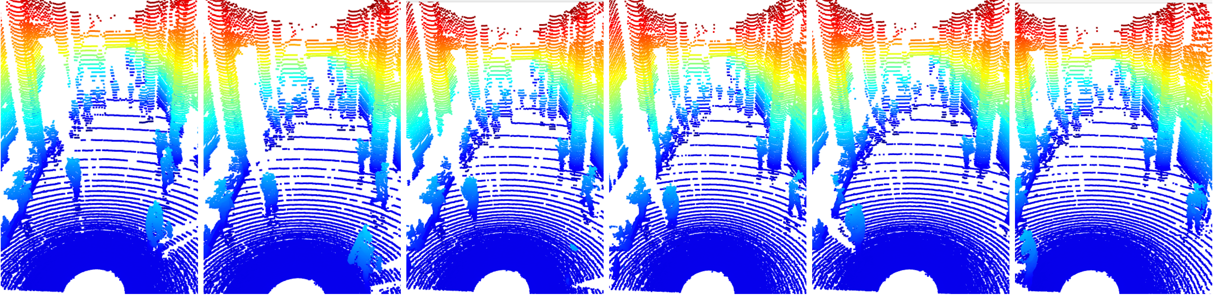
(a) An enclosed indoor corridor with pedestrians walking parallel to the robot’s direction of motion.

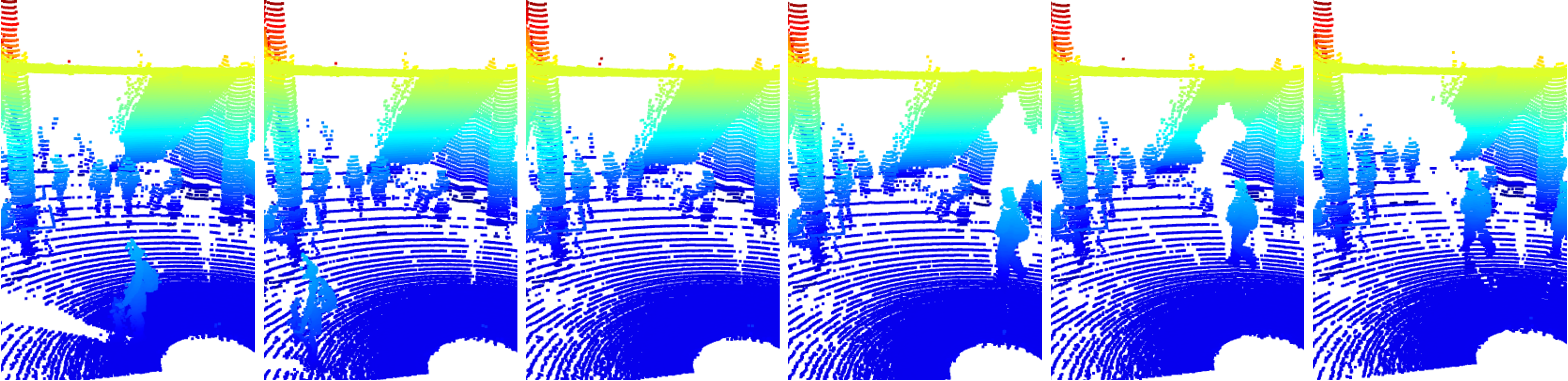
(b) An indoor intersection with complex pedestrian trajectories.

Figure 5: Indoor dataset: We collected over 200K raw point cloud frames(was down-sampled to around 23000 frames in training) at two indoor locations, incorporating complex movements of the crowd and changes in the indoor scenery.

As we mentioned in the main text, the amount of data after downsampling is still large considering that we only collected this data in 2 scenes. This makes it easier for the model to learn domain-specific knowledge, and explains why the performance of our pre-trained model drops after using more than 50% of the data.

Appendix C Detailed pretraining and fine-tuning results

In this section, we explain more details about the results from our experiments on how different pretrained/from-scratch VAE and CFM combinations perform on each of the three subtasks, which, again, are high-beam LiDAR adaptation, indoor occupancy forecasting, and semantic occupancy forecasting. For LoRAhu2021loralowrankadaptationlarge , across all our downstream tasks, we choose rank of 128 and $\alpha$ of 128. Please check section E for details on this selection. All models present in this section are trained for 40 epochs.

C.1 High-beam adaptation and indoor occupancy forecasting

In Table 10 and Table 11, we organize the performance of each of the pretrain/from-scratch combinations (VAE pretrained and CFM pretrained and fine-tuned with LoRAhu2021loralowrankadaptationlarge , both pretrained and full-parameter fine-tuned, only CFM pretrained, and both from-scratch) for high-beam adaptation and indoor occupancy forecasting in terms of IoU. IoU is computed through inferring the trained CFM model with NFE=10. Justification on this decision of this value of NFE is shown in section F.4. For high-beam adaptation task, pretrained CFM model is trained on original LiDAR sweeps, denoted by $G_{\theta}^{v}$. From the result, it is evident that full-parameter pretrained (both or only-CFM, with or without LoRA) yields exceeding performance over from-scratch trainings. Specifically, At 10% of fine-tuning data usage, our pretrained model with full-parameter fine-tuning achieves more than 14.48% relative performance improvement (more than 1.5% absolute performance improvement) across the three-second forecasting horizon and even at 100% data usage, our model still offers an absolute performance growth of about 1%. This demonstrates the effectiveness of our pretrained foundational in transferring geometric knowledge learned from 32 beams LiDAR data to tasks that demands different geometric properties (64 beams in this case) at different availability of fine-tuning data.

For indoor occupancy forecasting task, we use the same pretrained CFM model as the high-beam adaptation task. From the result, it is shown that at low fine-tuning data availability (10% and 25%), our pretrained models achieve exceeding performance over the from-scratch training. But when the amount of fine-tuning data increases to more than 50%, the from-scratch training obtains comparable or even better performance. Again, we explain this performance threshold to be resulting from the fine-tuning data amount over-rides the pretraining data and the lack of variance in the geometry of indoor occupancy dataset collected.

Table 10: High-beam adaptation fine-tuning results.

Data Fraction	Horizon	LoRA	Full-parameter	Only CFM-pretrained	Train from scratch
10%	1s	18.57	20.69	19.23	16.42
	2s	14.03	15.11	14.09	12.27
	3s	11.77	12.33	11.49	10.77
25%	1s	22.70	21.74	20.45	18.53
	2s	16.68	16.23	14.97	13.92
	3s	13.77	13.03	12.00	11.69
50%	1s	23.70	22.78	21.95	21.43
	2s	17.70	17.17	16.21	15.84
	3s	14.60	14.02	13.17	13.01
100%	1s	24.16	24.50	24.00	23.40
	2s	18.50	18.28	17.66	17.32
	3s	15.39	14.93	14.16	14.08

Table 11: Indoor occupancy forecasting fine-tuning results.

Data Fraction	Horizon	LoRA	Full-parameter	Only CFM-pretrained	Train from scratch
10%	1s	29.40	30.40	29.73	27.28
	2s	26.60	26.45	25.82	24.96
	3s	25.41	24.99	24.23	23.92
25%	1s	33.06	33.38	32.90	32.34
	2s	28.70	29.36	28.70	29.10
	3s	26.93	27.55	26.70	27.44
50%	1s	33.58	34.27	34.08	35.13
	2s	28.97	30.19	29.73	31.24
	3s	27.11	28.21	27.71	29.17
100%	1s	34.49	35.64	35.32	36.52
	2s	30.11	31.71	31.07	32.50
	3s	28.18	29.60	28.98	30.48

C.2 Semantic Occupancy Forecasting

For semantic occupancy forecasting task, the pretrained CFM model is trained on densified LiDAR frames, denoted by $G_{\theta}^{d}$. The results with numerical value of mIoU and IoU for different pretrained/from-scratch VAE and CFM combinations (NFE=10) at different fine-tuning data fraction are presented in table LABEL:table:_sem_occ_data. It is shown that at 10% of fine-tuning data utilization, our pretrained VAE and CFM with full-parameter fine-tuning provides a 11.17% absolute forecasting performance improvement in mIoU. In general, even the performance gain decays as the amount of fine-tuning data usage increases (which makes sense as it is getting closer and closer to the amount of pretraining data), the effectiveness of our foundational model prevails across all fine-tuning data fractions (at 100%, we still have about 1% performance improvement over the from-scratch model). One key thing to note is that we only fine-tune/train-from-scratch our semantic occupancy forecasting model with half of the available semantic labels for nuScenes (50% of the data used for the same task for other baseline models). This additional splitting of the training set is to prevent the overlap between pretrain and fine-tuning data in terms of geometric structure, as both densified occupancy forecasting and semantic occupancy forecasting models share the same set of scenes and the difference is that semantic occupancy forecasting data is labeled by category. This means that at 10% of fine-tuning data usage, having both VAE and CFM full-parameter fine-tuned based on our foundational model is able to achieve comparable performance with training-from-scratch and OccWorld (<$\pm 1.5\%$ absolute performance difference in both IoU and mIoU across three-second forecasting horizon) with only 5% of the data it consumes. Please refer to section H for visualizations of the forecasting results.

Table 12: Breakdown of fine-tuning results on the semantic occupancy task.

Data Fraction	Forecasting Horizon	LoRA		Full-parameter		Only CFM Pretrain		From Scratch
		IoU	mIoU	IoU	mIoU	IoU	mIoU	IoU	mIoU
10%	1s	35.92	23.29	36.24	24.69	36.05	24.09	27.00	13.52
	2s	26.01	14.19	26.17	14.91	25.61	14.63	19.41	8.25
	3s	20.60	9.80	20.87	10.42	20.24	10.21	15.81	6.14
25%	1s	37.21	27.42	37.85	28.88	36.64	27.80	33.84	22.73
	2s	27.46	17.23	27.09	17.58	26.95	17.03	24.62	13.65
	3s	22.04	12.31	21.36	12.30	21.61	11.84	19.29	9.38
50%	1s	37.17	28.47	38.40	30.84	37.09	28.23	37.02	28.10
	2s	27.59	17.48	27.81	19.00	27.53	17.64	27.30	17.50
	3s	22.31	12.44	22.14	13.62	22.29	12.58	21.80	12.34
100%	1s	37.13	28.83	38.91	31.64	36.59	28.39	38.21	30.54
	2s	27.80	17.56	28.58	19.59	27.46	18.01	28.22	19.06
	3s	22.65	12.52	23.13	14.22	22.50	13.02	22.31	13.45

Appendix D More details on representation alignment

As we mentioned before, during the pre-training phase, we found that it is more appropriate to use new data in fine-tuning the original VAE as opposed to training a VAE from scratch, even though the performance of our vae trained from scratch was excellent. We attribute this to the fact that the pre-trained generative model is in fact more adapted to the data distribution of the original latent, whereas the subspace structure of a latent learned from scratch with fine-tuned data would in fact be very different.

Specifically, for sub-task 3 (nonsemantic to semantic transfer), we cannot directly fine-tune the VAE considering the inconsistent size of the embeddng layers. Instead, we use the approach in Fig. 7: considering that $\bm{o}_{s}$ and $\bm{o}_{d}$ match one-to-one, and the original VAE is fine-tuned on $\bm{o}_{d}$, we can directly constrain the direct outputs of the encoder - mu and sigma. Previous work has tried to use bidirectional KL or EMD distance as a loss, but this does not work in our case: the data for the two modalities are in fact very close, differing only by semantic information.

Table 13: Comparison of feature alignment metrics before and after alignment.

	Dual KL	EMD	CKA	CKNNA	CosSim
Dense-Sem feature	0.004	0.008	0.739	0.278	0.183
Dense-Sem(Aligned) feature	0.002	0.004	0.944	0.410	0.907

Therefore we compared the latent from pair-wise $\bm{o}_{d}$ and $\bm{o}_{s}$ in line 1 of Table 13. We can see that both Dual-KL and EMD is very close, only cosine similarity is very different, which actually shown us that the most significant difference in the latent learned from these two VAEs is in fact the direction of the high-dimensional tensors. Then after use cosine similarity to constain the $\bm{o}_{s}$ VAE learning, the result is shown in line 2. With the tensor orientation restriction, we can successfully align the latent of the two VAEs, and the subsequent generative model training demonstrates that our alignment scheme can further improve the results.

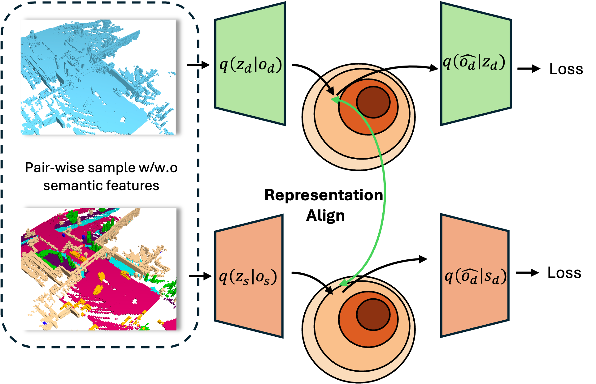
Figure 6: Use pretrained VAE for $\bm{o}_{d}$ to implicitly guide the structure of $\bm{o}_{s}$ latent space

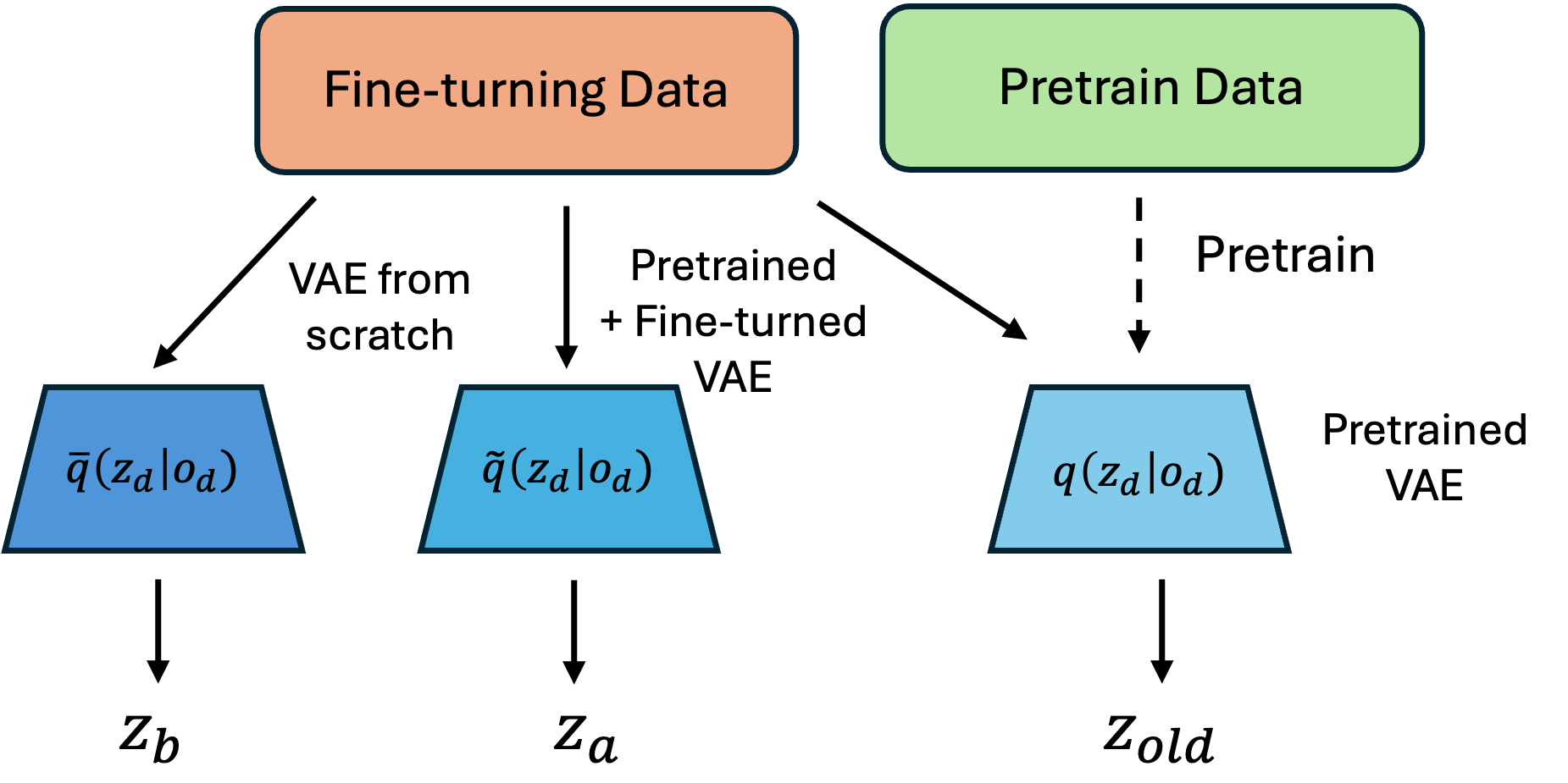
Figure 7: The comparison of latent space structure for non-paired data(in subtask 1 and 2)

For different beam lidar adaptation and outdoor-indoor generalization, while we can directly fine-tune the VAE, we cannot directly compare the similarity of the subspaces (CKAkornblith2019similarityneuralnetworkrepresentations and CKNNAhuh2024platonic require the same or similar samples as inputs to different networks). Our solution is shown in Figure 7. First, we use the original pretrained VAE, denoted by $q(z_{d}|o_{d})$ to get the latent of fine-tuning data without any training(adaption), denoted by $\bm{z}_{old}$. Then use the fine-tuned and training from scratch VAE to obtain the $\bm{z}_{b}$ and $\bm{z}_{a}$. If our hypothesise is correct, the distance between $(z_{a},z_{old})$ should smaller than $(z_{b},z_{old})$.

As data shown in Table D and LABEL:table:task2_vae, we listed the $(z_{a},z_{old})$ and $(z_{b},z_{old})$ in every 2 continuous lines for different fraction of fine-tuning data. We observe that with the increase of data amount used to fine-tuning the VAE, we do can have better result in terms of IOU, even better (when use 100% high beam KITTI data) or very close to the pretrained one. However, what really determines the forecast performance is actually the similarity between the latent space after fine-tuning the VAE and the latent space after only pretrain. Compared to training from scratch, the latent space after fine-tuning the VAE is more similar to the latent produced by using pretrain weight directly, which allows for better use of knowledge from the foundational model. In other words, fine-tuning the VAE is in fact about leaving the original latent space as unaltered as possible while allowing the weights of the original VAE to be adapted (and accurately compressed) to the new sample.

Table 14: VAE fine-tuning evaluation in different beam adaptation

Pretrain	Fine-tuning	IoU	CKA	CKNNA
$\bm{o}_{v}$	10% KITTI	97.97	0.661	0.231
$\varnothing$	10% KITTI	85.08	0.477	0.171
$\bm{o}_{v}$	25% KITTI	98.16	0.625	0.214
$\varnothing$	25% KITTI	88.66	0.489	0.188
$\bm{o}_{v}$	50% KITTI	98.31	0.610	0.211
$\varnothing$	50% KITTI	90.79	0.495	0.188
$\bm{o}_{v}$	100% KITTI	98.40	0.611	0.208
$\varnothing$	100% KITTI	98.46	0.494	0.189

Table 15: VAE fine-tuning evaluation in outdoor to indoor adaptation.

Pretrain	Fine-tuning	IoU	CKA	CKNNA
$\bm{o}_{d}$	10% Indoor	95.82	0.739	0.245
$\varnothing$	10% Indoor	88.77	0.592	0.186
$\bm{o}_{d}$	25% Indoor	96.65	0.720	0.233
$\varnothing$	25% Indoor	92.14	0.606	0.199
$\bm{o}_{d}$	50% Indoor	97.15	0.691	0.221
$\varnothing$	50% Indoor	94.09	0.611	0.203
$\bm{o}_{d}$	100% Indoor	98.18	0.688	0.220
$\varnothing$	100% Indoor	95.97	0.609	0.200

Appendix E Analysis on LoRA fine-tuning with different ranks

To determine the optimal LoRAhu2021loralowrankadaptationlarge configuration for our downstream tasks, we tested the following ranks: 32, 64, and 128 with $\alpha=rank$ and dropout rate of 0.05 on semantic occupancy forecasting subtask with 10% of fine-tuning data and both VAE and CFM components pretrained as explained earlier. We apply LoRA only to the Linear layers, embedding layers, 2D and 3D convolution layers in the CFM architecture. The training is done for 40 epochs for LoRA and full-parameter fine-tuning baseline. The goal of this mini-scale experiment is to find the balance between model performance and parameter efficiency. The result is shown in table 16. First, after sampling the CFM, the model yields suboptimal performance under rank of 32 and 64, with 3.51% and 2.48% absolute performance gap with the full-parameter fine-tuning in terms of mean mIoU across three-second forecasting horizon, respectively. This indicates that the model does not acquire satisfactory level of semantic information from fine-tuning data within the 40 epochs training process which might be caused by lack of depth in the LoRA layers. On the other hand, rank of 128 demonstrates performance that is closest to the full-parameter fine-tuning: 0.25% less in mean IoU and 0.91% less in mean mIoU. This shows that rank of 128 offers enough depth for information to be extracted from the semantic occupancy data and demonstrate comparable performance against the baseline. This rank and $\alpha$ combination is what we present earlier for all downstream tasks under the "LoRA" fine-tuning category.

We did not test any higher or lower rank because: since rank of 32 and 64 both has considerable performance gap compared to the full-parameter fine-tuning, lower rank means less parameters (depth) for LoRA layers which means the model is less likely to learn useful information from the fine-tuning data and consequently, is unlikely to achieve comparable performance with the full-parameter method; on the other hand, rank of 128 already has 10.21 million trainable parameters in total where our CFM model alone only has 11.51 million parameters. This means that under such rank, we are fine-tuning about the same number of parameter as the full-parameter fine-tuning approach. This more-or-less makes experiment the model performance with higher LoRA rank redundant because we will be fine-tuning even more parameters than vanilla fine-tuning and the key advantage of LoRA is to fine-tune the model with optimal performance and reduced trainable parameters. With that said, we tried rank of 32, 64, and 128 and utilizes rank=128 variation for all LoRA fine-tuning completed for our downstream tasks.

Table 16: Comparison of different LoRA configurations (rank and $\alpha$ values) and full parameter fine-tuning for semantic occupancy forecasting task. We report the method type, number of trainable parameters, mean IoU, and mean mIoU. Note that our full-parameter CFM models only have 11.51 M parameters, excluding VAE which has 18.86 M parameters.

Method	Rank	$\alpha$	Parameters (M)	mean IoU ↑	mean mIoU ↑
Full-parameter	-	-	11.51	27.76	16.67
LoRA	32	32	2.55	26.27	13.16
LoRA	64	64	5.10	27.14	14.19
LoRA	128	128	10.21	27.51	15.76

Appendix F Additional ablation studies

F.1 The data efficiency of proposed VAE structure

Follow the official splitting of train/validation set in nuScenes, we test the proposed VAE performance under different fraction of training data. As shown in Table 17, our method only need half of the training data to exceed all of previous data compressor, as we mentioned in the abstract.

Table 17: Performance of proposed VAE under different training data fraction, under 192x compression rate, 100 epochs training

Data fraction	IOU	mIOU
$100\%$	85.8	93.8
$50\%$	83.4	92.1
$25\%$	82.0	90.2
$10\%$	78.9	85.8

F.2 Results of forecasting on pretraining data

In our setting, we use $\bm{o}_{v}$ (Sparse voxels) as pretraining data for sparse-dense beam lidar adaptation, and $\bm{o}_{d}$ (Densified voxels) for the rest of 2 subtasks. Here in Table 18, we show the IOU of these 2 pretraining models which will be used as "foundational" models later.

Table 18: Pretraining performance on different LiDAR representations, without future trajectory.

Dataset	IoU$\uparrow$
	1s	2s	3s	Avg
$\bm{o}_{v}$	26.98	21.56	18.26	22.27
$\bm{o}_{d}$	39.64	29.35	23.73	30.91

Considering the sparsity, it’s naturally more difficult to have a accurate forecast result under $O_{v}$, as the undensified point clouds to lead to a "swimming" effect of points on the surface of objects.

F.3 VAE and forecasting result break down

Table 19: Per-class IoU and overall metrics across different semantic occupancy compression models.

Method	Comp.	mIoU	IoU	Others	Barrier	Bicycle	Bus	Car	Const. Veh.	Motorcycle	Pedestrian	Traffic Cone	Trailer	Truck	Drive. Surf.	Other Flat	Sidewalk	Terrain	Man-made	Vegetation
OccWorldzheng2024occworld	16	65.7	62.2	45.0	72.2	69.6	68.2	69.4	44.4	70.7	74.8	67.6	56.1	65.4	82.7	78.4	69.7	66.4	52.8	43.7
OccSorawang2024occsora	512	27.4	37.0	11.7	22.6	0.0	34.6	29.0	16.6	8.7	11.5	3.5	20.1	29.0	61.3	38.7	36.5	31.1	12.0	18.4
OccLLAMAwei2024occllama	16	75.2	63.8	65.0	87.4	93.5	77.3	75.1	60.8	90.7	88.6	91.6	67.3	73.3	81.1	88.9	74.7	71.9	48.8	42.4
DOMEgu2024dome	64	83.1	77.3	36.6	90.9	95.9	85.8	92.0	69.1	95.3	96.8	92.5	77.5	85.6	93.6	94.2	89.0	85.5	72.2	58.7
Ours	192	93.8	85.8	89.5	97.8	97.5	93.7	96.0	86.2	98.4	97.6	97.6	92.1	94.7	97.2	98.5	95.8	94.8	84.6	73.6

In Table 19, we present the compression performance of the proposed VAE across different semantic categories. With a 3× compression ratio, our method consistently outperforms prior approaches in all categories. Notably, for rare classes such as Construction Vehicle, Trailer, and Vegetation, our model achieves improvements of 22.2%, 18.8%, and 25.4% over DOME’s VAE, respectively. These results indicate that our VAE effectively mitigates the impact of data imbalance across categories in the compression process.

Table 20: 3 seconds average per-class IoU for semantic occupancy forecasting

Method	mIoU	IoU	Others	Barrier	Bicycle	Bus	Car	Const. Veh.	Motorcycle	Pedestrian	Traffic Cone	Trailer	Truck	Drive. Surf.	Other Flat	Sidewalk	Terrain	Man-made	Vegetation
OccWorldzheng2024occworld	17.13	26.63	12.23	20.77	8.27	20.50	19.86	12.58	7.89	8.95	8.45	13.04	17.73	35.09	23.65	23.97	20.66	17.01	20.17
Ours(Hist. Traj.)	23.33	31.78	21.41	23.70	15.33	26.00	23.05	27.44	13.19	10.29	13.10	21.89	24.85	40.68	30.99	29.29	26.64	21.52	26.57
DOMEgu2024dome	22.18	32.13	19.84	25.66	15.36	21.03	21.98	23.96	11.36	7.99	14.79	18.02	21.58	39.84	30.46	28.74	25.35	23.01	27.22
Ours(Fut. Traj.)	28.49	37.52	28.38	33.77	19.99	29.81	28.17	32.46	18.76	12.08	20.78	25.59	30.85	43.27	34.01	32.65	29.34	30.10	34.26

Now, we present a per-category performance analysis. In Table 20, we compare the average IOU for 3s under each category. Compared to OccWorldzheng2024occworld , our improvement in forecasting performance for medium-sized objects is particularly significant: we improve the forecasts of bicycle, Const. Veh. and Motorcycle by 85.36%, 118.12% and 67.17%, respectively. A broadly performance gain also observed when include future trajectory as condition, the top 2 improvement categories are also small object, relatively 65.18% and 51.2% for Motorcycle and Pedestrian respectively.

F.4 NFE selection for CFM solver during inference

To determine the optimal NFE for our CFM solver during inference, we experiment how the performance and efficiency of our proposed VAE plus CFM architecture for semantic occupancy forecasting vary for different values of NFE. Specifically, for NFE values, we start with NFE=100 and do the decrement of 50, 25, 10, and 5. For performance, as we are performing semantic occupancy forecasting, we infer our model with the corresponding NFE and record mean IoU and mIoU for comparison. For efficiency, we collect two key metrics: Gflops per frame and frame per second for one iteration of sampling that produces 6 frames with 2 Hz of frequency. The results for this experiment is depicted by figure 8.

According to the result, in terms of performance, it is shown model performance does not scale up with NFE. In contrast, we can see that NFE=10 offers the best value of mIoU and second-best value of IoU (0.1% behind the best one at NFE=25). Evaluating efficiency in terms of Gflops and FPS, Gflops per frame increases and FPS decreases with increasing NFE, which suggests the negative correlation between efficiency and NFE. Since NFE=10 gives the best overall performance, we can also observe that it has the second-best efficiency metric overall. For the sampling of our efficiency latent flow matching framework, we want to emphasize model performance and efficiency at the same time to allow better real-world implementation. Thus, based on the result, we choose NFE=10 for all the model inference process.

Figure 8: The performance and efficiency of proposed VAE + CFM architecture under different NFE value during the sampling process. We observe that NFE=10 corresponds to the best model performance, with reasonable efficiency in terms of FPS and Gflops per frame.

F.5 Model performance with different fractions of pretraining data

In the previous content we showed that based on the foundational model, the performance boost when we increase the fine-tuning data amount and also the result w/w.o the foundational model. But another question is whether the performance of the model improves with the inclusion of more pretraining data? We designed a simple experiment to answer this question.

Figure 9: Performance improvement from different ratios of pretraining data

We choose 25% of fine-tuning data for 3 different subtasks to simplify the fine-tuning. In Fig. 9, 100% data on the x-axis represents the full pretraining data $O_{v}$. We observe a clear performance improvement (relative improvements of 21.9% , 22.2% and 12.9% for indoor occupancy forecasting, semantic occupancy forecasting and high-beam adaptation tasks) as the amount of pretraining data varies from 50% of $O_{v}$ to 100%.

F.6 CFM performance sensitivity analysis with sampling randomization

The inference process of flow matching is essentially solving the Probability Flow ODE(PF-ODE) as mentioned by previous worksong2023consistency , which is actually deterministic given the sampled Gaussian noise is fixed. Here we also provide a experiment to illustrate this stability. Specifically, using Euler solver, we evaluate the two foundational models (sparse and dense occupancy forecasting) and semantic occupancy forecasting model with 5 random seeds and record the average and standard deviation for IoU and mIoU across the three-second forecasting horizon (on the validation data). We present the results in Table 21, and note that the standard deviation of the performance metrics for all three models is less than 1% of the mean across the entire forecasting horizon. Therefore, we conclude that our CFM model has low performance sensitivity to randomization in the sampling process and the uncertainty around the performance metrics evaluated is minimal.

Table 21: Different CFM models and their average IoU/mIoU (±std) over a three-second horizon, tested with 5 different random seeds.

Model trained on	IoU$\uparrow$				mIoU$\uparrow$
	1s	2s	3s	Avg	1s	2s	3s	Avg
$O_{v}$	26.67$\pm$0.02	21.56$\pm$0.01	18.26$\pm$0.02	22.26$\pm$0.02	–	–	–	–
$\bm{o}_{d}$	39.82$\pm$0.13	29.34$\pm$0.04	23.73$\pm$0.07	30.93$\pm$0.01	–	–	–	–
$O_{s}$	40.64$\pm$0.10	30.31$\pm$0.06	24.21$\pm$0.17	31.72$\pm$0.04	33.57$\pm$0.28	21.15$\pm$0.05	14.99$\pm$0.46	23.25$\pm$0.06

Appendix G Limitation and future work

Physical consistency. Although our method achieves state-of-the-art performance across different time horizons, the issue of continuous consistency in generated videos remains unresolved. For foreground objects, The current solution only achieves smooth output by performing timing processing within the network structure, but in the generated scenes, especially foreground objects, are still prone to discontinuities. As shown in Table 20, although our work has greatly improved the accuracy of the forecasting foreground objects, there is still no theoretical or design guarantee that the foreground object will be continuous in the output (i.e., it will not suddenly appear or disappear in a few frames).

Multi-agent trajectory forecasting For a safe end-to-end autonomous driving system, it is still very difficult for the current occupancy world model to not only decode the occupancy map after obtaining the future representation, but also forecast the future multi-modal trajectories of surrounding agents. This involves not only the efficient detection of foreground objects and the aforementioned consistency forecasting, but also how to introduce future possibilities into ODE-based sampling methods such as flow matching. We hope that this work will provide an efficient implementation framework for solving this issues in the future and accelerate the progress of subsequent work.

Appendix H Visualization

H.1 Samples from the pretrained model

Here we visualize the forecasting results for two of the foundational models that are pretrained. Specifically, visualization for sparse occupancy forecasting is shown in figure 10 and visualization for dense occupancy forecasting is shown in figure 11.

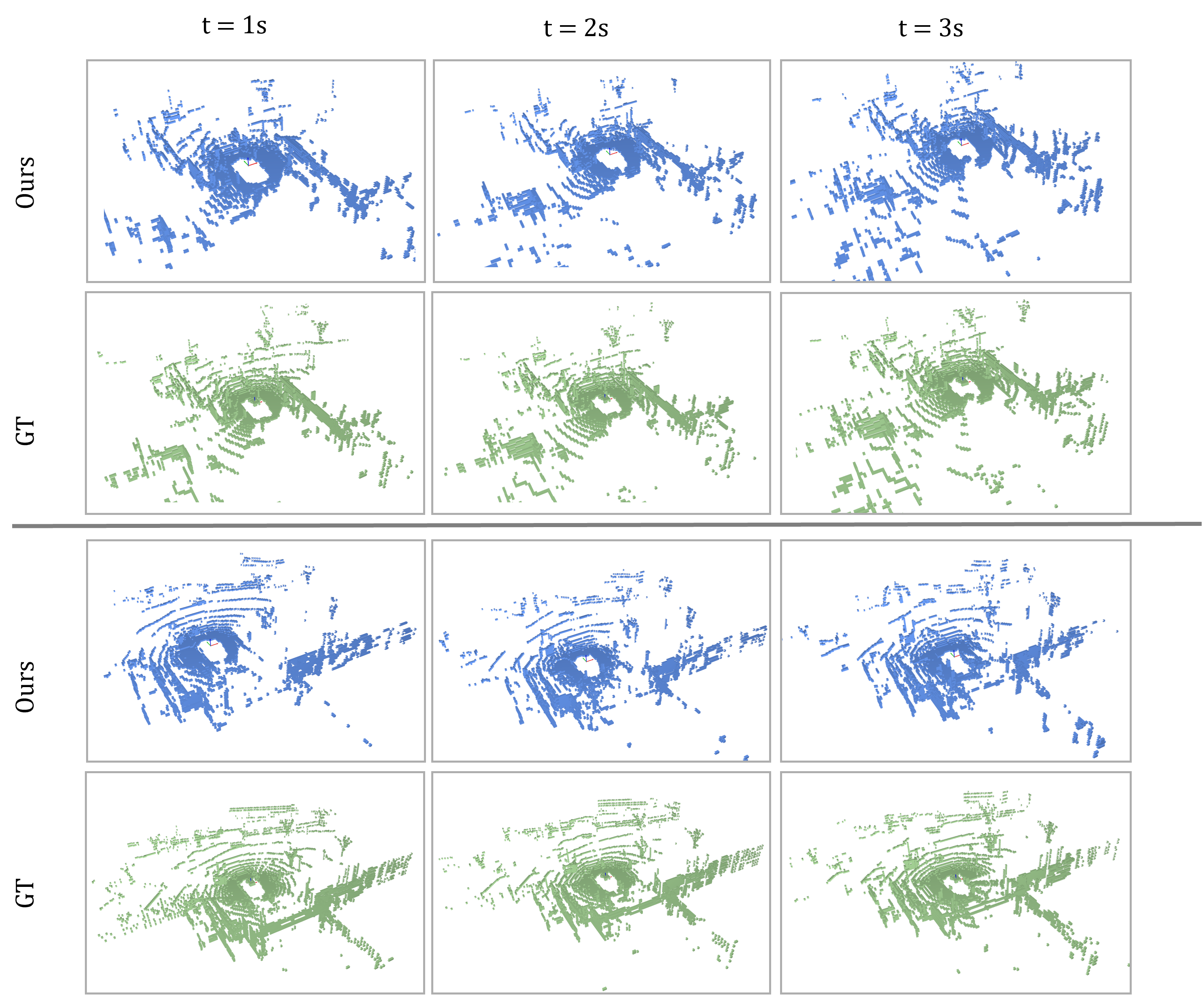
Figure 10: Visualization for the sparse occupancy($O_{v}$) forecasting over the three-second forecasting horizon.

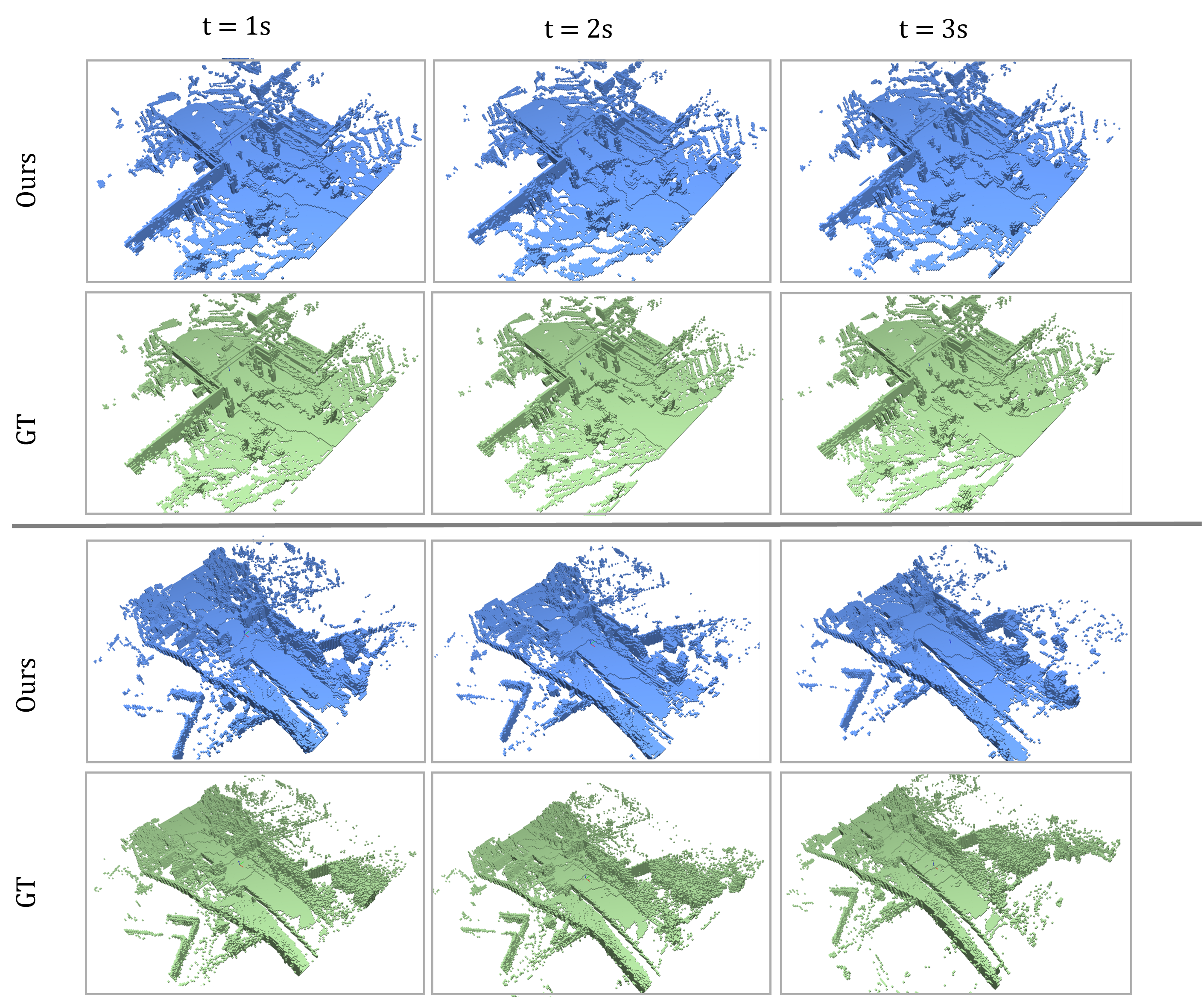
Figure 11: Visualization for the dense occupancy($\bm{o}_{d}$) forecasting over the three-second forecasting horizon.

H.2 Samples from the semantic occupancy forecasting model

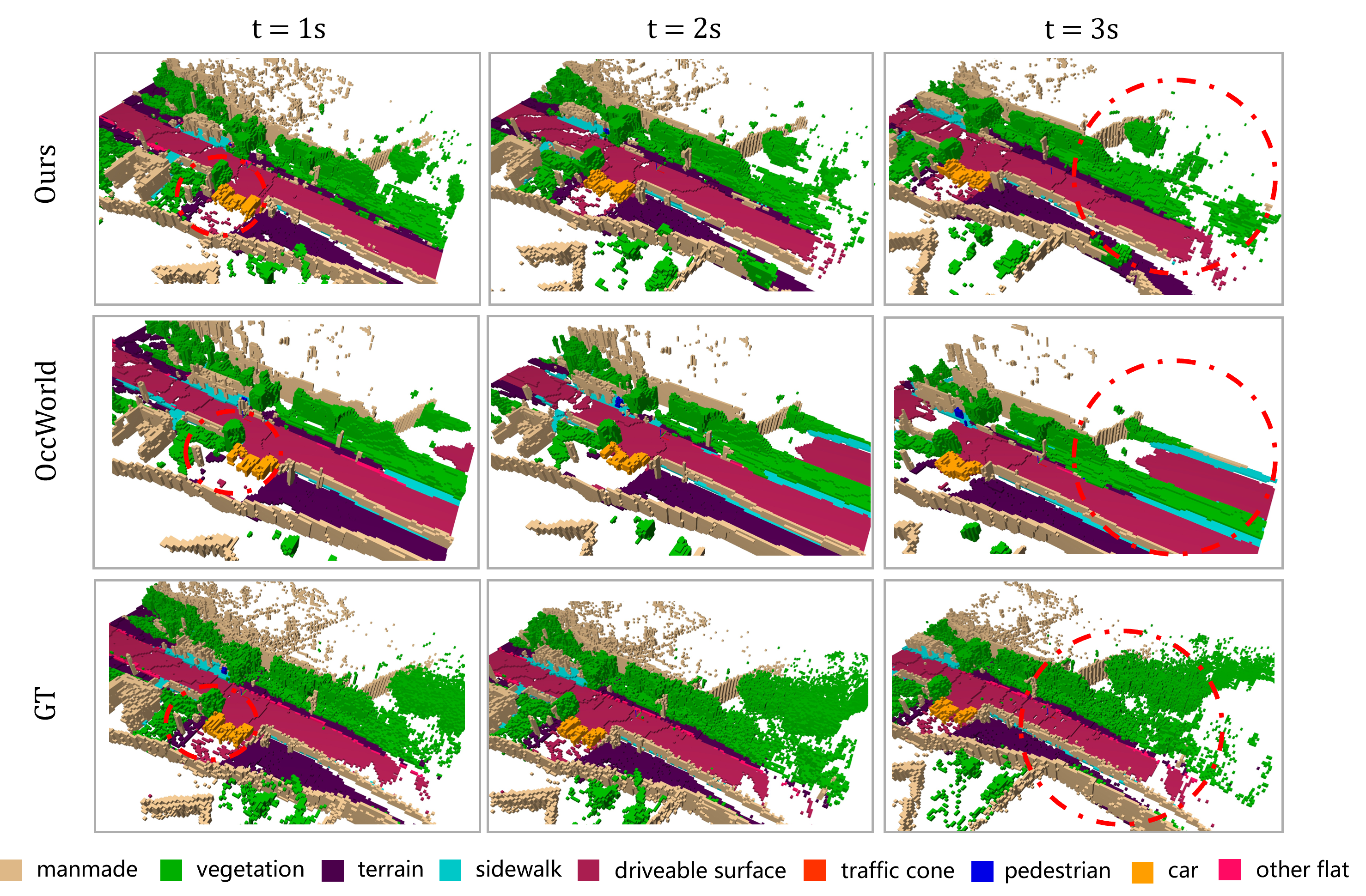
Figure 12: Visualization for the semantic occupancy($O_{s}$) forecasting over the three-second forecasting horizon. Compared to the previous method, our method retains more details in this example (as shown in the red circle)

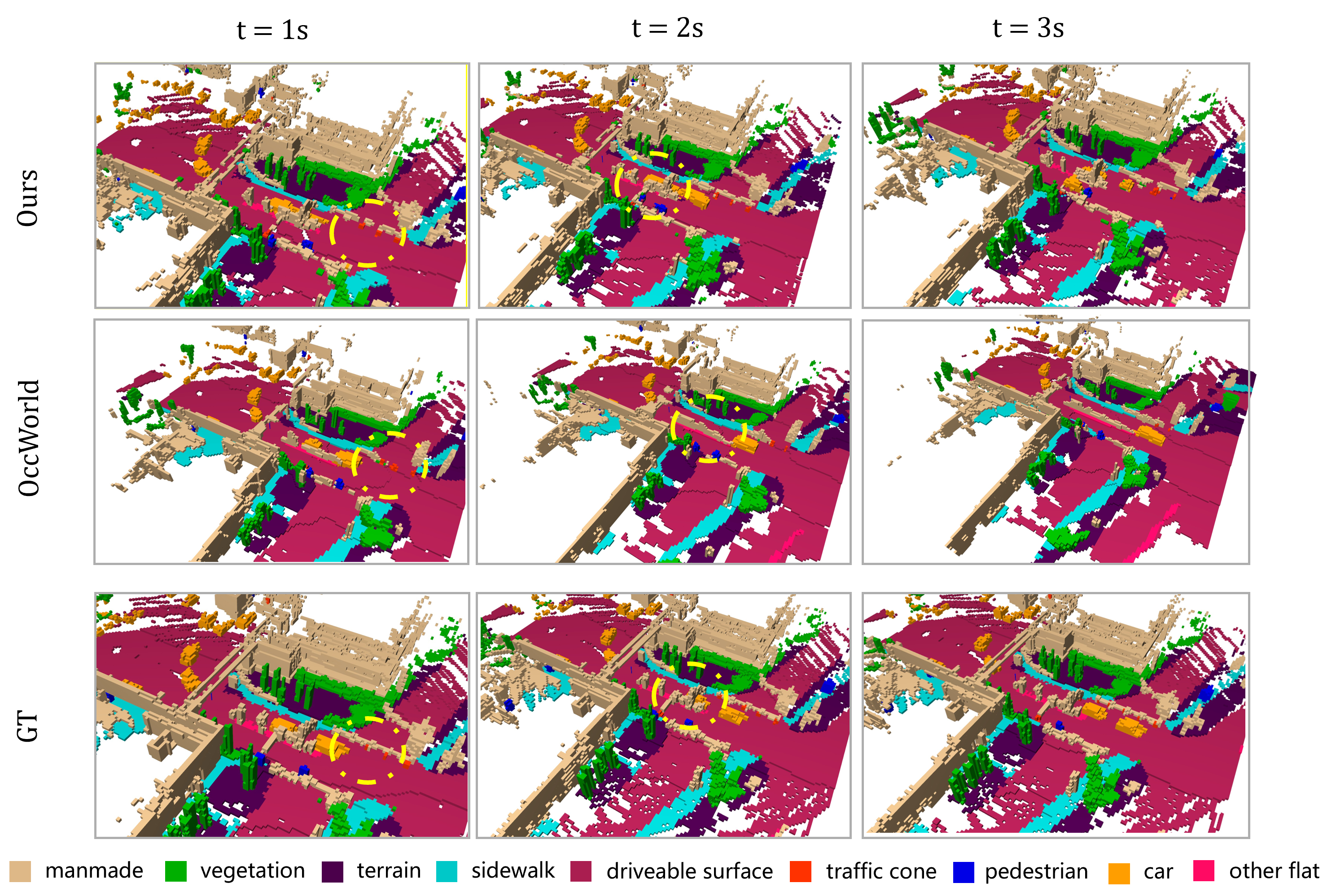
Figure 13: Visualization for the semantic occupancy($O_{s}$) forecasting over the three-second forecasting horizon for an intersection. Compared to the previous method, as shown by the yellow circle, our methods better forecasts foreground (close-ranged) objects such as cars and barriers.

References

- [1] Niket Agarwal, Arslan Ali, Maciej Bala, Yogesh Balaji, Erik Barker, Tiffany Cai, Prithvijit Chattopadhyay, Yongxin Chen, Yin Cui, Yifan Ding, et al. Cosmos world foundation model platform for physical ai. arXiv preprint arXiv:2501.03575, 2025.
- [2] Ben Agro, Quinlan Sykora, Sergio Casas, Thomas Gilles, and Raquel Urtasun. Uno: Unsupervised occupancy fields for perception and forecasting. In Proceedings of the IEEE/CVF Conference on Computer Vision and Pattern Recognition, pages 14487–14496, 2024.
- [3] Hassan Abu Alhaija, Jose Alvarez, Maciej Bala, Tiffany Cai, Tianshi Cao, Liz Cha, Joshua Chen, Mike Chen, Francesco Ferroni, Sanja Fidler, et al. Cosmos-transfer1: Conditional world generation with adaptive multimodal control. arXiv preprint arXiv:2503.14492, 2025.
- [4] Amir Bar, Gaoyue Zhou, Danny Tran, Trevor Darrell, and Yann LeCun. Navigation world models. arXiv preprint arXiv:2412.03572, 2024.
- [5] Maxim Berman, Amal Rannen Triki, and Matthew B Blaschko. The lovász-softmax loss: A tractable surrogate for the optimization of the intersection-over-union measure in neural networks. In Proceedings of the IEEE conference on computer vision and pattern recognition, pages 4413–4421, 2018.
- [6] Hengwei Bian, Lingdong Kong, Haozhe Xie, Liang Pan, Yu Qiao, and Ziwei Liu. Dynamiccity: Large-scale lidar generation from dynamic scenes. arXiv preprint arXiv:2410.18084, 2024.
- [7] Kevin Black, Noah Brown, Danny Driess, Adnan Esmail, Michael Equi, Chelsea Finn, Niccolo Fusai, Lachy Groom, Karol Hausman, Brian Ichter, et al. : A vision-language-action flow model for general robot control. arXiv preprint arXiv:2410.24164, 2024.
- [8] Ang Cao and Justin Johnson. Hexplane: A fast representation for dynamic scenes. In Proceedings of the IEEE/CVF Conference on Computer Vision and Pattern Recognition, pages 130–141, 2023.
- [9] Ricky T. Q. Chen, Yulia Rubanova, Jesse Bettencourt, and David Duvenaud. Neural ordinary differential equations, 2019.
- [10] Christopher Choy, JunYoung Gwak, and Silvio Savarese. 4d spatio-temporal convnets: Minkowski convolutional neural networks. In Proceedings of the IEEE/CVF conference on computer vision and pattern recognition, pages 3075–3084, 2019.
- [11] Patrick Esser, Sumith Kulal, Andreas Blattmann, Rahim Entezari, Jonas Müller, Harry Saini, Yam Levi, Dominik Lorenz, Axel Sauer, Frederic Boesel, et al. Scaling rectified flow transformers for high-resolution image synthesis. In Forty-first international conference on machine learning, 2024.
- [12] Will Grathwohl, Ricky T. Q. Chen, Jesse Bettencourt, Ilya Sutskever, and David Duvenaud. Ffjord: Free-form continuous dynamics for scalable reversible generative models. In International Conference on Learning Representations (ICLR), 2019.
- [13] Songen Gu, Wei Yin, Bu Jin, Xiaoyang Guo, Junming Wang, Haodong Li, Qian Zhang, and Xiaoxiao Long. Dome: Taming diffusion model into high-fidelity controllable occupancy world model. arXiv preprint arXiv:2410.10429, 2024.
- [14] James R Han, Hugues Thomas, Jian Zhang, Nicholas Rhinehart, and Timothy D Barfoot. Dr-mpc: Deep residual model predictive control for real-world social navigation. IEEE Robotics and Automation Letters (RA-L), 2025.
- [15] Anthony Hu, Lloyd Russell, Hudson Yeo, Zak Murez, George Fedoseev, Alex Kendall, Jamie Shotton, and Gianluca Corrado. Gaia-1: A generative world model for autonomous driving. arXiv preprint arXiv:2309.17080, 2023.
- [16] Edward J. Hu, Yelong Shen, Phillip Wallis, Zeyuan Allen-Zhu, Yuanzhi Li, Shean Wang, Lu Wang, and Weizhu Chen. Lora: Low-rank adaptation of large language models, 2021.
- [17] Minyoung Huh, Brian Cheung, Tongzhou Wang, and Phillip Isola. The platonic representation hypothesis. arXiv preprint arXiv:2405.07987, 2024.
- [18] Tero Karras, Miika Aittala, Timo Aila, and Samuli Laine. Elucidating the design space of diffusion-based generative models. Advances in neural information processing systems, 35:26565–26577, 2022.
- [19] Tarasha Khurana, Peiyun Hu, David Held, and Deva Ramanan. Point cloud forecasting as a proxy for 4d occupancy forecasting. In IEEE/CVF Conference on Computer Vision and Pattern Recognition (CVPR), 2023.
- [20] Moo Jin Kim, Karl Pertsch, Siddharth Karamcheti, Ted Xiao, Ashwin Balakrishna, Suraj Nair, Rafael Rafailov, Ethan Foster, Grace Lam, Pannag Sanketi, Quan Vuong, Thomas Kollar, Benjamin Burchfiel, Russ Tedrake, Dorsa Sadigh, Sergey Levine, Percy Liang, and Chelsea Finn. Openvla: An open-source vision-language-action model, 2024.
- [21] Simon Kornblith, Mohammad Norouzi, Honglak Lee, and Geoffrey Hinton. Similarity of neural network representations revisited, 2019.
- [22] Bohan Li, Jiazhe Guo, Hongsi Liu, Yingshuang Zou, Yikang Ding, Xiwu Chen, Hu Zhu, Feiyang Tan, Chi Zhang, Tiancai Wang, et al. Uniscene: Unified occupancy-centric driving scene generation. arXiv preprint arXiv:2412.05435, 2024.
- [23] Zhuoling Li, Xiaogang Xu, SerNam Lim, and Hengshuang Zhao. Towards unified 3d object detection via algorithm and data unification. arXiv preprint arXiv:2402.18573, 2024.
- [24] Yiyi Liao, Jun Xie, and Andreas Geiger. Kitti-360: A novel dataset and benchmarks for urban scene understanding in 2d and 3d. IEEE Transactions on Pattern Analysis and Machine Intelligence, 45(3):3292–3310, 2022.
- [25] Xingchao Liu, Chengyue Gong, and Qiang Liu. Flow straight and fast: Learning to generate and transfer data with rectified flow. arXiv preprint arXiv:2209.03003, 2022.
- [26] Xinhao Liu, Moonjun Gong, Qi Fang, Haoyu Xie, Yiming Li, Hang Zhao, and Chen Feng. Lidar-based 4d occupancy completion and forecasting. In 2024 IEEE/RSJ International Conference on Intelligent Robots and Systems (IROS), pages 11102–11109. IEEE, 2024.
- [27] Zhen Luo, Junyi Ma, Zijie Zhou, and Guangming Xiong. Pcpnet: An efficient and semantic-enhanced transformer network for point cloud prediction. IEEE Robotics and Automation Letters, 8(7):4267–4274, 2023.
- [28] Xin Ma, Yaohui Wang, Gengyun Jia, Xinyuan Chen, Ziwei Liu, Yuan-Fang Li, Cunjian Chen, and Yu Qiao. Latte: Latent diffusion transformer for video generation. arXiv preprint arXiv:2401.03048, 2024.
- [29] Björn Michele, Alexandre Boulch, Tuan-Hung Vu, Gilles Puy, Renaud Marlet, and Nicolas Courty. Train till you drop: Towards stable and robust source-free unsupervised 3d domain adaptation. In European Conference on Computer Vision, pages 1–19. Springer, 2024.
- [30] Ben Mildenhall, Pratul P Srinivasan, Matthew Tancik, Jonathan T Barron, Ravi Ramamoorthi, and Ren Ng. Nerf: Representing scenes as neural radiance fields for view synthesis. Communications of the ACM, 65(1):99–106, 2021.
- [31] Kazuto Nakashima, Xiaowen Liu, Tomoya Miyawaki, Yumi Iwashita, and Ryo Kurazume. Fast lidar data generation with rectified flows. arXiv preprint arXiv:2412.02241, 2024.
- [32] Lucas Nunes, Rodrigo Marcuzzi, Benedikt Mersch, Jens Behley, and Cyrill Stachniss. Scaling diffusion models to real-world 3d lidar scene completion. In Proceedings of the IEEE/CVF Conference on Computer Vision and Pattern Recognition, pages 14770–14780, 2024.
- [33] William Peebles and Saining Xie. Scalable diffusion models with transformers. In Proceedings of the IEEE/CVF international conference on computer vision, pages 4195–4205, 2023.
- [34] Haoxi Ran, Vitor Guizilini, and Yue Wang. Towards realistic scene generation with lidar diffusion models. In Proceedings of the IEEE/CVF Conference on Computer Vision and Pattern Recognition, pages 14738–14748, 2024.
- [35] Robin Rombach, Andreas Blattmann, Dominik Lorenz, Patrick Esser, and Björn Ommer. High-resolution image synthesis with latent diffusion models. In Proceedings of the IEEE/CVF conference on computer vision and pattern recognition, pages 10684–10695, 2022.
- [36] Lloyd Russell, Anthony Hu, Lorenzo Bertoni, George Fedoseev, Jamie Shotton, Elahe Arani, and Gianluca Corrado. Gaia-2: A controllable multi-view generative world model for autonomous driving. arXiv preprint arXiv:2503.20523, 2025.
- [37] Yang Song, Prafulla Dhariwal, Mark Chen, and Ilya Sutskever. Consistency models. 2023.
- [38] Yang Song, Jascha Sohl-Dickstein, Diederik P. Kingma, Abhishek Kumar, Stefano Ermon, and Ben Poole. Score-based generative modeling through stochastic differential equations. In International Conference on Learning Representations (ICLR), 2021.
- [39] Xiaoyu Tian, Tao Jiang, Longfei Yun, Yucheng Mao, Huitong Yang, Yue Wang, Yilun Wang, and Hang Zhao. Occ3d: A large-scale 3d occupancy prediction benchmark for autonomous driving. Advances in Neural Information Processing Systems, 36:64318–64330, 2023.
- [40] Lening Wang, Wenzhao Zheng, Yilong Ren, Han Jiang, Zhiyong Cui, Haiyang Yu, and Jiwen Lu. Occsora: 4d occupancy generation models as world simulators for autonomous driving. arXiv preprint arXiv:2405.20337, 2024.
- [41] Xiaofeng Wang, Zheng Zhu, Wenbo Xu, Yunpeng Zhang, Yi Wei, Xu Chi, Yun Ye, Dalong Du, Jiwen Lu, and Xingang Wang. Openoccupancy: A large scale benchmark for surrounding semantic occupancy perception. In Proceedings of the IEEE/CVF International Conference on Computer Vision, pages 17850–17859, 2023.
- [42] Yuqi Wang, Jiawei He, Lue Fan, Hongxin Li, Yuntao Chen, and Zhaoxiang Zhang. Driving into the future: Multiview visual forecasting and planning with world model for autonomous driving. In Proceedings of the IEEE/CVF Conference on Computer Vision and Pattern Recognition, pages 14749–14759, 2024.
- [43] Julong Wei, Shanshuai Yuan, Pengfei Li, Qingda Hu, Zhongxue Gan, and Wenchao Ding. Occllama: An occupancy-language-action generative world model for autonomous driving. arXiv preprint arXiv:2409.03272, 2024.
- [44] Xinshuo Weng, Junyu Nan, Kuan-Hui Lee, Rowan McAllister, Adrien Gaidon, Nicholas Rhinehart, and Kris M Kitani. S2net: Stochastic sequential pointcloud forecasting. In European Conference on Computer Vision, pages 549–564. Springer, 2022.
- [45] Benjamin Wilson, William Qi, Tanmay Agarwal, John Lambert, Jagjeet Singh, Siddhesh Khandelwal, Bowen Pan, Ratnesh Kumar, Andrew Hartnett, Jhony Kaesemodel Pontes, et al. Argoverse 2: Next generation datasets for self-driving perception and forecasting. arXiv preprint arXiv:2301.00493, 2023.
- [46] Yuwen Xiong, Wei-Chiu Ma, Jingkang Wang, and Raquel Urtasun. Ultralidar: Learning compact representations for lidar completion and generation. arXiv preprint arXiv:2311.01448, 2023.
- [47] Ziyang Yan, Wenzhen Dong, Yihua Shao, Yuhang Lu, Liu Haiyang, Jingwen Liu, Haozhe Wang, Zhe Wang, Yan Wang, Fabio Remondino, et al. Renderworld: World model with self-supervised 3d label. arXiv preprint arXiv:2409.11356, 2024.
- [48] Lunjun Zhang, Yuwen Xiong, Ze Yang, Sergio Casas, Rui Hu, and Raquel Urtasun. Copilot4d: Learning unsupervised world models for autonomous driving via discrete diffusion. arXiv preprint arXiv:2311.01017, 2023.
- [49] Yumeng Zhang, Shi Gong, Kaixin Xiong, Xiaoqing Ye, Xiao Tan, Fan Wang, Jizhou Huang, Hua Wu, and Haifeng Wang. Bevworld: A multimodal world model for autonomous driving via unified bev latent space. arXiv preprint arXiv:2407.05679, 2024.
- [50] Wenzhao Zheng, Weiliang Chen, Yuanhui Huang, Borui Zhang, Yueqi Duan, and Jiwen Lu. Occworld: Learning a 3d occupancy world model for autonomous driving. In European conference on computer vision, pages 55–72. Springer, 2024.
- [51] Lipu Zhou, Daniel Koppel, and Michael Kaess. Lidar slam with plane adjustment for indoor environment. IEEE Robotics and Automation Letters, 6(4):7073–7080, 2021.
- [52] Yang Zhou, Hao Shao, Letian Wang, Steven L Waslander, Hongsheng Li, and Yu Liu. Smartpretrain: Model-agnostic and dataset-agnostic representation learning for motion prediction. arXiv preprint arXiv:2410.08669, 2024.