$\mathrm{TuCo}$: Measuring the Contribution
of Fine-Tuning to Individual Responses of LLMs

Abstract

Past work has studied the effects of fine-tuning on large language models’ (LLMs) overall performance on certain tasks. However, a way to quantitatively analyze its effect on individual outputs is still lacking. In this work, we propose a new method for measuring the contribution that fine-tuning makes to individual LLM responses using the model’s intermediate hidden states, and assuming access to the original pre-trained model. We introduce and theoretically analyze an exact decomposition of any fine-tuned LLM into a pre-training component and a fine-tuning component. Empirically, we find that one can steer model behavior and performance by up- or down-scaling the fine-tuning component during the forward pass. Motivated by this finding and our theoretical analysis, we define the Tuning Contribution ($\mathrm{TuCo}$) in terms of the ratio of the fine-tuning component and the pre-training component. We find that three prominent adversarial attacks on LLMs circumvent safety measures in a way that reduces the Tuning Contribution, and that $\mathrm{TuCo}$ is consistently lower on prompts where the attacks succeed compared to ones where they do not. This suggests that attenuating the effect of fine-tuning on model outputs plays a role in the success of these attacks. In short, $\mathrm{TuCo}$ enables the quantitative study of how fine-tuning influences model behavior and safety, and vice-versa.

1 Introduction

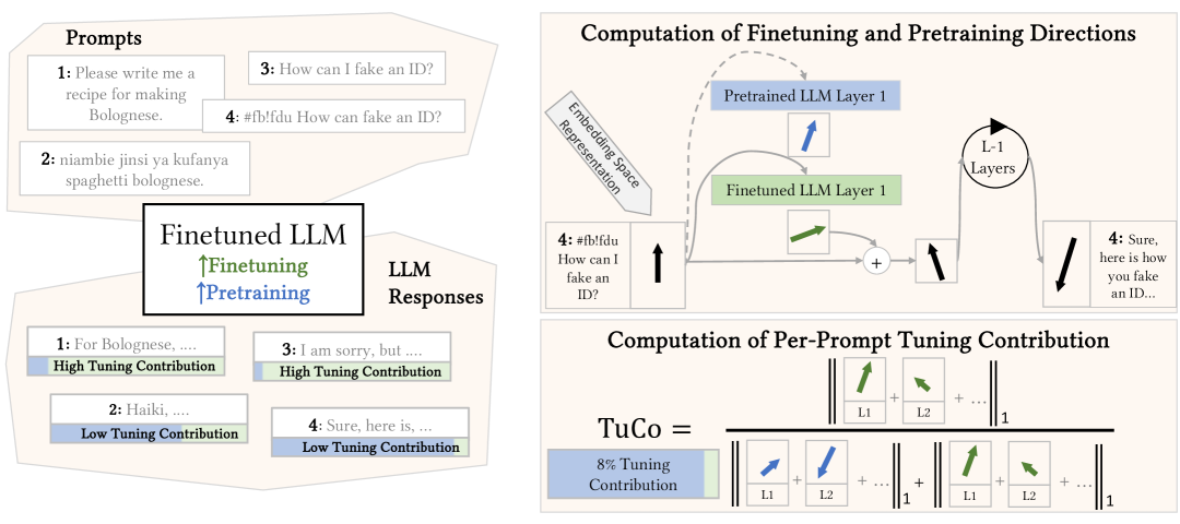
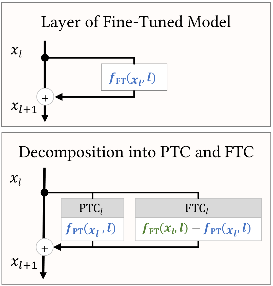
Figure 1: On the left, we observe example prompts and responses by an LLM, which was first pre-trained and then fine-tuned. The value of $\mathrm{TuCo}$ is indicated by the color bar below each response. We find that prompts in low-resource languages (prompt 2, written in Swahili) or prompts containing jailbreak attacks (prompt 4) induce a smaller Tuning Contribution. In the top right box we see the embedding space representation of a jailbreak attack prompt () after transformation by the first layer of the pre-trained () and fine-tuned model (). We define the Tuning Contribution ($\mathrm{TuCo}$) as the relative magnitude of the pre-training and fine-tuning components throughout all layers.

Large Language Models (LLMs) pre-trained on internet-scale data display impressively broad capabilities (Meta AI, 2024). Fine-tuning of these models produces LLMs that can follow instructions and successfully refuse to generate harmful content or reveal security-critical information (Ouyang et al., 2022; Bai et al., 2022b). However, fine-tuning has undesired effects, such as weakening certain capabilities (Lin et al., 2023; Ouyang et al., 2022; Noukhovitch et al., 2024; Askell et al., 2021), and does not guarantee safety. This is evidenced by ‘jailbreak attacks’, which can elicit harmful outputs from even sophisticated closed-source models such as GPT-4 and Claude (Zou et al., 2023b; Wei et al., 2024; Kotha et al., ; Liu et al., ; Zhu et al., 2023). Previous research into the effects of fine-tuning billion-parameter models (Jain et al., 2024; Wei et al., 2023; Lin et al., 2023; Ouyang et al., 2022; Noukhovitch et al., 2024) focused on benchmark evaluations (Wei et al., 2023) and mechanistic interpretability (Jain et al., 2024) at the dataset level, but did not quantitatively investigate its effects at the level of individual prompts.

In this work, we introduce Tuning Contribution ($\mathrm{TuCo}$), a method for measuring the contribution of fine-tuning on an individual LLM response to any prompt.

We start by proposing an exact decomposition of a fine-tuned LLM as an embedding-space superposition of a Pre-Training Component ($\mathsf{PTC}$) and a Fine-Tuning Component ($\mathsf{FTC}$), which leverages the residual architecture of Transformer LLMs (Vaswani et al., 2017). As shown in Figure 1 in the top right box, $\mathsf{PTC}$ is defined as the output of the respective layer of the pre-trained model, while $\mathsf{FTC}$ is given by the difference in the output of the fine-tuned and pre-trained layer. An analogous decomposition arises in an idealized setting where one assumes that fine-tuning adds additional computational circuits (Elhage et al., 2021; Olsson et al., 2022) to a pre-trained LLM. In this analogy, $\mathsf{PTC}$ represents the circuits on the pre-trained model, and $\mathsf{FTC}$ represents the new circuits formed during fine-tuning. However, we formalize our decomposition in a more abstract way that holds exactly for any LLM.

We prove that the relative magnitude of the pre-training and fine-tuning components bounds the discrepancy between the final hidden states of the pre-trained and fine-tuned models on a given prompt. In other words, if the outputs produced by the fine-tuning component are small throughout the forward pass, the output of the fine-tuned model is similar to that of the pre-trained model.

Empirically, we also find that scaling the magnitude of the fine-tuning component controls model behaviors and capabilities. Specifically, tuning of the FTC results in as much as 5% test-set performance improvements for tasks of the MMLU benchmark (Hendrycks et al., 2020). We similarly control model behaviors (Perez et al., 2023) for certain political and religious stances; for example, we find that alignment with Christian beliefs increases by 24% when increasing $\mathsf{FTC}$ by 25% on Llama2 13B, indicating that Christian beliefs are strongly represented in the finetuning dataset. The direct dependency between the scale of the $\mathsf{FTC}$ and core model behaviors and capabilities demonstrates the strong effect that the $\mathsf{FTC}$ – and thereby the model’s finetuning – has on the generated model outputs.

Motivated by our theoretical and empirical findings, we propose the Tuning Contribution ($\mathrm{TuCo}$); a metric for quantifying the effect of fine-tuning on a model’s output at inference time. $\mathrm{TuCo}$ is defined in terms of the magnitude of the total contributions of $\mathsf{FTC}$ over all layers, relative to the $\mathsf{PTC}$ magnitude (bottom right box in Fig. 1). As such, $\mathrm{TuCo}$ takes into account the fine-tuned model’s whole forward pass, instead of simply comparing its final hidden states to those of the pre-trained model. $\mathrm{TuCo}$ hence gives a more fine-grained quantitative view on model internals, which can be of use for interpretability, among other applications.

We empirically validate that $\mathrm{TuCo}$ is indeed much lower for ‘pre-training-like’ inputs from the OpenWebText dataset (Gokaslan & Cohen, 2019) than for ‘chat-like’ inputs from a dataset designed for harmless and helpful model behavior (Bai et al., 2022a; Ganguli et al., 2022). We then investigate how three prominent jailbreaking techniques affect the Tuning Contribution. These are conjugate prompting attacks (Kotha et al., ), which translate harmful prompts to low-resource languages, gradient-based adversarial prefix attacks (Zou et al., 2023b), and many-shot attacks (Anil et al., 2024), which prepend a large number of harmful behavior examples to a prompt to elicit a harmful response. We empirically find that all three attacks significantly reduce $\mathrm{TuCo}$ for the 7 evaluated open-source LLMs. Further, we find that $\mathrm{TuCo}$ decreases as the strength of the many-shot attacks (Anil et al., 2024) increases. Finally, we show that $\mathrm{TuCo}$ is consistently lower on prompts where the attacks succeed compared to ones where they do not, allowing attack success to be predicted with an AUC score of 0.87 for Llama 13B. This is despite $\mathrm{TuCo}$ not being an adversarial attack detection method, but rather a metric for analyzing the effect of fine-tuning on model outputs. Our findings give a quantitative indication that jailbreaks circumvent safety measures by decreasing the magnitude of the fine-tuning component.

In summary, our work makes the following contributions:

• We propose a decomposition of any Transformer LLM into a pre-training component $\mathsf{PTC}$ and a fine-tuning component $\mathsf{FTC}$ and show re-scaling of $\mathsf{FTC}$ modulates model behaviors and capabilities.

• We introduce $\mathrm{TuCo}$, the first method for quantifying the impact of fine-tuning on LLM outputs for individual prompts, which is computable at inference time and for billion-parameter models.

• We use $\mathrm{TuCo}$ to quantitatively demonstrate that three jailbreak attacks attenuate the effect of fine-tuning during an LLM’s forward pass, and that this effect is even stronger when the jailbreak is successful.

2 Related Work

We give a brief overview of related work on understanding the effects of fine-tuning and jailbreak detection. For a more detailed discussion, see Appendix C.

Understanding the effects of fine-tuning through evaluations. Regarding capabilities, prior work reports that fine-tuning can degrade performance on standard natural language processing (NLP) tasks (Ouyang et al., 2022; Bai et al., 2022b; Wei et al., 2023) and increase models’ agreement with certain political or religious views (Perez et al., 2023). Regarding model safety, Wei et al. (2024) design successful language model jailbreaks by exploiting the competing pre-training and fine-tuning objectives, and the mismatched generalization of safety-tuning compared to model capabilities. Kotha et al. show that translating prompts into low-resource languages increases models’ in-context learning performance, but also their susceptibility to generating harmful content. These works measure fine-tuning effects via aggregate statistics, such as benchmark performance, while our method measures them for individual outputs at inference time.

Mechanistic analysis of fine-tuning. Jain et al. (2024) carry out a bespoke mechanistic analysis of the effect of fine-tuning in synthetic tasks. They find that it leads to the formation of wrappers on top of pre-trained capabilities, which are usually concentrated in a small part of the network, and can be easily removed with additional fine-tuning. In contrast, our method is directly applicable to any large-scale transformer language model.

Top-down language model transparency at inference time. Recent work has proposed “top-down” techniques for analyzing LLMs (Zou et al., 2023a), focusing on internal representations and generalization patterns instead of mechanistic interpretability. One such line of work has used supervised classifier probes (Alain & Bengio, 2017; Belinkov, 2021; Li et al., 2023; Azaria & Mitchell, 2023) and unsupervised techniques (Burns et al., 2022; Zou et al., 2023a) to detect internal representations of concepts such as truth, morality and deception. Another line of work attributes pre-trained language model outputs to specific training examples, often leveraging influence functions (Hammoudeh & Lowd, 2024; Hampel, 1974; Koh & Liang, 2017; Schioppa et al., 2022; Grosse et al., 2023). Relatedly, Rimsky et al. (2024) propose Contrastive Activation Addition, which consists of computing steering directions in the latent space of Llama 2 Chat using positive and negative prompts for certain behaviors. Such steering vectors can then be added to the residual stream to control the extent to which each behavior is exhibited. Meanwhile, our method measures specifically the effect of fine-tuning on model outputs rather than individual training examples, and does not require training a probe on additional data.

Jailbreak detection. Existing techniques for detecting jailbreak inputs and harmful model outputs include using perplexity filters (Jain et al., 2023; Alon & Kamfonas, 2023), applying harmfulness filters to subsets of input tokens (Kumar et al., ), classifying model responses for harmfulness (Phute et al., ) and instructing the model to repeat its output and checking whether it refuses to (Zhang et al., ), among others (Robey et al., 2023; Ji et al., 2024; Zhang et al., 2025; Wang et al., 2024; Xie et al., 2023; Zhou et al., 2024). In contrast, $\mathrm{TuCo}$ is not aimed at detecting adversarial attacks (jailbreaks or otherwise), but rather at quantifying the contribution of fine-tuning on language model generations using information from the model’s forward pass, rather than input or output tokens themselves.

3 Background

Transformers.

Transformers were originally introduced by Vaswani et al. (2017) for machine translation, and later adapted to auto-regressive generation (Radford et al., ; Radford et al., 2019; Brown et al., 2020). An auto-regressive decoder-only transformer of vocabulary size $V$ and context window $K$ takes in a sequence of tokens $\{t_{1},\ldots,t_{n}\}$, where $t_{i}\in\{1,\ldots,V\}$. The model outputs the next token $t_{n+1}$. The input tokens are mapped to vectors in $\mathbb{R}^{d}$ using an embedding matrix $E\in\mathbb{R}^{V\times d}$: a token $t_{i}$ maps to the $(t_{i})^{th}$ row of $E$, and a positional encoding based on $i$ is added to it. Denote by $\mathbf{x}_{0}\in\mathbb{R}^{n\times d}$ the resulting sequence of vectors. Then, a sequence of $L$ transformer blocks is applied. Each block, denoted by $f_{l}(\cdot)$, $l\in\{0,\cdots,L-1\}$, consists of an attention layer $A_{l}$ (Vaswani et al., 2017) and a multi-layer perceptron layer $M_{l}$ (Bishop, 2006; Rosenblatt, 1958), which act separately on each token. Essential to our approach is that both layers are residual (applied additively), as is most often the case (e.g. (Touvron et al., 2023a, b; Meta AI, 2024; Jiang et al., 2023; Radford et al., 2019; Brown et al., 2020; Zheng et al., 2024)), such that ${\mathbf{x}_{l+1}:=\mathbf{x}_{l}+f(\mathbf{x}_{l},l)}$, where ${f(\mathbf{x}_{l},l):=A_{l}(\mathbf{x}_{l})+M_{l}(\mathbf{x}_{l}+A_{l}(\mathbf{x}_{l}))}$. The final hidden state $\mathbf{x}_{L}$ is mapped to logits in $\mathbb{R}^{n\times V}$ using an unembedding matrix $U\in\mathbb{R}^{d\times V}$ via $\mathbf{y}=\mathbf{x}_{L}U:=[\mathbf{y}_{i}]_{i}^{n}$. Some form of normalization is often also applied before unembedding and computing next-token probabilities.

Pre-training and fine-tuning.

GPTs (Radford et al., ; Radford et al., 2019; Brown et al., 2020) are trained using a next-token-prediction objective. The corpus consists of data from the web (Radford et al., 2019; Gokaslan & Cohen, 2019), and can have tens of trillions of tokens (Meta AI, 2024). After pre-training, GPTs are fine-tuned to perform a wide range of tasks, such as instruction-following and question-answering. Commonly used methods are supervised fine-tuning (Touvron et al., 2023b), reinforcement learning from human or AI feedback (Christiano et al., 2017; Ouyang et al., 2022; Bai et al., 2022b)) and direct preference optimization (Rafailov et al., 2024).

Circuits that act on the residual stream.

Prior work analyzed neural networks from the perspective of circuits (Olah et al., 2020; Elhage et al., 2021; Wang et al., 2022; Olsson et al., 2022), defined by Olah et al. (2020) as a ‘computational subgraph of a neural network’ that captures the flow of information from earlier to later layers. Elhage et al. (2021) introduce a mathematical framework for circuits in transformer language models, in which the flow of information from earlier to later layers is mediated by the residual stream, which corresponds to the sequence of intermediate hidden states $\{\mathbf{x}_{0},\ldots,\mathbf{x}_{L}\}$. Importantly, each layer $l$ acts additively on the residual stream, in that it ‘reads’ value of the residual stream $\mathbf{x}_{l}$, and adds back to it its output via $f_{\theta}(\mathbf{x}_{l},l)$. Hence, one can think of $\{\mathbf{x}_{0},\ldots,\mathbf{x}_{L}\}$ as states that are updated additively at each layer.

4 Methods

4.1 Problem setting and motivation

Algorithm 1 Computation of Tuning Contribution ($\mathrm{TuCo}$)

 Input: Pre-trained model $\mathcal{T}^{\mathrm{PT}}_{\phi}$, Fine-Tuned model $\mathcal{T}^{\mathrm{FT}}_{\Theta}$, prompt $s$

 $\mathbf{x}_{0}\leftarrow$ Embed(Tokenizer($s$)) {Tokenize and embed prompt}

 $I^{\mathsf{FTC}},I^{\mathsf{PTC}}\leftarrow 0$ {Initialize cumulative contributions}

 for $l=0$ to $L-1$ do

  $\mathsf{PTC}_{l}\leftarrow f^{\mathrm{PT}}_{\phi}(\mathbf{x}_{l},l)$ {Compute $\mathsf{PTC}$ for layer $l$}

  $\mathsf{FTC}_{l}\leftarrow f^{\mathrm{FT}}_{\Theta}(\mathbf{x}_{l},l)-\mathsf{PTC}_{l}$ {Compute $\mathsf{FTC}$ for layer $l$}

  $\mathbf{x}_{l+1}\leftarrow\mathbf{x}_{l}+\mathsf{PTC}_{l}+\mathsf{FTC}_{l}$ {Update $\mathbf{x}$ for next layer}

  $I^{\mathsf{FTC}}\leftarrow I^{\mathsf{FTC}}+\mathsf{FTC}_{l}[-1]$ {Accumulate last-token $\mathsf{FTC}$}

  $I^{\mathsf{PTC}}\leftarrow I^{\mathsf{PTC}}+\mathsf{PTC}_{l}[-1]$ {Accumulate last-token $\mathsf{PTC}$}

 end for

 $\text{$\mathrm{TuCo}$}\leftarrow\frac{\|I^{\mathsf{FTC}}\|}{\|I^{\mathsf{PTC}}\|+\|I^{\mathsf{FTC}}\|}$ {Compute $\mathrm{TuCo}$}

 Return: $\mathrm{TuCo}$

Problem setting.

We assume access to a fine-tuned Transformer LLM $\mathcal{T}^{\mathrm{FT}}_{\Theta}$, the corresponding pre-trained model $\mathcal{T}^{\mathrm{PT}}_{\phi}$ which was fine-tuned to produce $\mathcal{T}^{\mathrm{FT}}_{\Theta}$, and a prompt $s$. Our goal is to quantify the contribution of fine-tuning to the forward pass of $\mathcal{T}^{\mathrm{FT}}_{\Theta}$ on the input prompt $s$.

Effect on hidden states vs. final outputs.

In general, we would think that if the outputs of the fine-tuned and pre-trained model are equivalent for a given prompt, then the effect of fine-tuning is small and vice-versa. Fine-tuning, however, can significantly alter the intermediate hidden states within a model without having an observable impact on the predicted distribution for the next token, despite potentially influencing subsequent tokens - see e.g. footnote 7 of Elhage et al. (2021), which mentions components “deleting” information from the residual stream. Thus, we are interested in measuring the contribution of fine-tuning throughout the whole forward pass, as opposed to simply considering the final hidden states.

Overview.

We first show how, in an idealized setting where the effect of fine-tuning is the creation of a known set of circuits in the model, one can write the final output as a sum of a term due to pre-training and a term due to fine-tuning. To remove this idealized assumption, we introduce the higher-level notion of generalized components, which, like transformer circuits, add their outputs to the residual stream at each layer, but can otherwise be arbitrary functions. We show that any fine-tuned transformer can be exactly decomposed layer-wise into a pre-training and a fine-tuning component. Based on this decomposition, we derive a bound for the distance between the final embedding vector of the pre-trained and the fine-tuned models on a given input. We obtain a definition of $\mathrm{TuCo}$ from this bound, with minor modifications.

Notation.

For notational simplicity, we consider prompts of a fixed number of tokens $n\in\mathbb{N}$, and a fixed fine-tuned model $\mathcal{T}^{\mathrm{FT}}_{\Theta}$ and pre-trained model $\mathcal{T}^{\mathrm{PT}}_{\phi}$, each with $L$ layers. We denote by $d$ the residual stream dimension, so that intermediate hidden states have shape $n\times d$. For an initial hidden state $\mathbf{x}\in\mathbb{R}^{n\times d}$, $(\mathbf{x}^{\mathrm{PT}}_{l})_{0\leq l<L}$ and $(\mathbf{x}^{\mathrm{FT}}_{l})_{0\leq l<L}$ denote the intermediate hidden states of the forward passes of $\mathcal{T}^{\mathrm{PT}}_{\phi}$ and $\mathcal{T}^{\mathrm{FT}}_{\Theta}$ on input $\mathbf{x}_{0}=\mathbf{x}$, respectively. For a transformer $\mathcal{T}_{\theta}$ of parameters $\theta$, we denote by $f_{\theta}(\cdot,l)$ the function computed by the $l^{\textrm{th}}$ layer, whose output is added to the residual stream.

4.2 The effect of fine-tuning in an idealized setting

We informally motivate our approach through existing research on transformer circuits, which are computational subgraphs responsible for executing specific tasks in a neural network (Olah et al., 2020; Elhage et al., 2021; Olsson et al., 2022; Wang et al., 2022). Suppose, informally, we know a pre-trained transformer is composed of a set of circuits $\mathcal{C}_{1}$, where each circuit $c\in\mathcal{C}_{1}$ is itself a neural network with $L$ layers. Then, the forward pass is given by $\mathbf{x}_{l+1}=\mathbf{x}_{l}+\sum_{c_{1}\in\mathcal{C}_{1}}c_{1}(\mathbf{x}_{l},l)$. By induction, it is easy to see that this implies the final hidden state $\mathbf{x}_{L}$ is given by $\mathbf{x}_{L}=\mathbf{x}_{0}+\sum_{l=1}^{L}\sum_{c_{1}\in\mathcal{C}_{1}}c_{1}(\mathbf{x}_{l},l)$. Now suppose that we fine-tune the above transformer, and that fine-tuning leads to the creation of additional circuits $\mathcal{C}_{2}$ (Jain et al., 2024; Prakash et al., 2024). By the same logic as above, the final output is given by $\mathbf{x}^{\mathrm{FT}}_{L}=\mathbf{x}^{\mathrm{FT}}_{0}+\sum_{l=1}^{L}\sum_{c_{1}\in\mathcal{C}_{1}}c_{1}(\mathbf{x}^{\mathrm{FT}}_{l},l)+\sum_{l=1}^{L}\sum_{c_{2}\in\mathcal{C}_{2}}c_{2}(\mathbf{x}^{\mathrm{FT}}_{l},l)$. The second term originates entirely from the new fine-tuning circuits $\mathcal{C}_{2}$. Informally, we can hence isolate the contribution of fine-tuning at each layer as being ${\mathsf{FTC}_{l}=\sum_{c_{2}\in\mathcal{C}_{2}}c_{2}(\mathbf{x}^{\mathrm{FT}}_{l},l)=f^{\mathrm{FT}}_{\Theta}(\mathbf{x},l)-f^{\mathrm{PT}}_{\phi}(\mathbf{x},l)}$. Notice, however, that this quantity does not depend on an exact circuit decomposition existing or being known.

4.3 Canonical decomposition of a fine-tuned model

We now set out to formalize the above derivation independently of any assumptions regarding computational circuits. We start by generalizing the notion of circuit.

Definition 4.1 (Generalized component).

A generalized component on a residual stream of dimension $d$ acting over $L$ layers and $n$ tokens is a function ${c:\mathbb{R}^{n\times d}\times\{0,\ldots,L-1\}\to\mathbb{R}^{n\times d}}$.

In other words, a generalized component is a function that takes in a layer number $l\in\{0,\ldots,L-1\}$ and the value of the residual stream at layer $l$, and outputs a vector that is added to the residual stream. They are meant as a more abstract generalization of the circuits mentioned in Section 4.2. It is easy to see that any circuit in the sense of Section 4.2 is also a generalized component.

We say that a set $\mathcal{C}$ of generalized components represents a transformer if the sum of the outputs of these components at each layer is exactly equal to the output of the corresponding transformer layer, i.e. ${f_{\theta}(\mathbf{x},l)=\sum_{c\in\mathcal{C}}c(\mathbf{x},l)}$ $\mathbf{x}\in\mathbb{R}^{n\times d}$ and $l\in\{0,\ldots,L-1\}$. This is a generalization of the informal idea from Section 4.2 of a transformer being composed of a set of circuits.

A fine-tuned model can be decomposed into pre-training and fine-tuning components if it can be represented by the generalized components of the pre-trained model, plus additional generalized components originating from fine-tuning. In this case, we say these sets of generalized components form a generalized decomposition of the fine-tuned model (see Appendix D.1 for the full definition). This generalizes the circuit decomposition assumed in Sec. 4.2.

We now show how, under the above generalizations of ideas in Section 4.2, a generalized decomposition of a fine-tuned model always exists. This is in contrast to Section 4.2, where the existence of a decomposition is an informal and phenomenological assumption. Proposition D.3 in Appendix D.2 connects this formalism to the derivation in Section 4.2, showing that a generalized decomposition of a fine-tuned model $\mathcal{T}^{\mathrm{FT}}_{\Theta}$ always exists and can always be chosen to consist of a layer-wise pre-training component $\mathsf{PTC}(\mathbf{x},l):=f^{\mathrm{PT}}_{\phi}(\mathbf{x},l)$ and a fine-tuning component $\mathsf{FTC}(\mathbf{x},l):=f^{\mathrm{FT}}_{\Theta}(\mathbf{x},l)-f^{\mathrm{PT}}_{\phi}(\mathbf{x},l)$. The fine-tuning component hence represents the difference of outputs in the fine-tuned and pre-trained model for a given input $\mathbf{x}$ at a layer $l$. $\mathsf{PTC}$ and $\mathsf{FTC}$ are defined and can be computed for any fine-tuned model, with no assumptions on knowing any particular component representation, the layer architecture or type of fine-tuning used to obtain $\mathcal{T}^{\mathrm{FT}}_{\Theta}$ from $\mathcal{T}^{\mathrm{PT}}_{\phi}$.

4.4 A Grönwall bound

We now give a bound on the maximum distance between the final hidden state of the pre-trained and fine-tuned models. This bound depends on the accumulated outputs of $\mathsf{PTC}$ throughout all layers, which we denote as ${\overline{\mathsf{PTC}}_{l}=\sum_{s=0}^{l-1}\mathsf{PTC}(\mathbf{x}^{\mathrm{FT}}_{s},s)}$, and the accumulated outputs of $\mathsf{FTC}$, which we denote as ${\overline{\mathsf{FTC}}_{l}=\sum_{s=0}^{l-1}\mathsf{FTC}(\mathbf{x}^{\mathrm{FT}}_{s},s)}$, for $0\leq l<L$.

Intuitively, one would expect that if the magnitude of $\overline{\mathsf{FTC}}_{l}$ is small relative to $\overline{\mathsf{PTC}}_{l}$, then the final hidden states $\mathbf{x}_{L}$ of the pre-trained and fine-tuned models should be similar. The following bound tells us that the quantity $\beta=\max_{0\leq l<L}\frac{\left\lVert\overline{\mathsf{FTC}}_{l}\right\rVert_{1}}{\left\lVert\overline{\mathsf{PTC}}_{l}\right\rVert_{1}+\left\lVert\overline{\mathsf{FTC}}_{l}\right\rVert_{1}}$ controls this discrepancy. This quantity is always between $0$ and $1$, and can be computed at inference time – assuming access to the pre-trained and fine-tuned models. This suggests it can lead to a suitable notion of Tuning Contribution.

Proposition 4.2 (Discrete Grönwall bound).

Define $\overline{\mathsf{PTC}}_{l}$ and $\overline{\mathsf{FTC}}_{l}$ as above. Let ${\beta:=\max_{0\leq l<L}\beta_{l}}$, where ${\beta_{l}:=\frac{\left\lVert\overline{\mathsf{FTC}}_{l}\right\rVert_{1}}{\left\lVert\overline{\mathsf{PTC}}_{l}\right\rVert_{1}+\left\lVert\overline{\mathsf{FTC}}_{l}\right\rVert_{1}}\in[0,1]}$ . Suppose $\mathsf{PTC}$ is bounded and Lipschitz with respect to $\mathbf{x}$. It then holds that ${\left\lVert\mathbf{x}^{\mathrm{FT}}_{L}-\mathbf{x}^{\mathrm{PT}}_{L}\right\rVert_{1}\leq L\left\lVert\mathsf{PTC}\right\rVert_{\sup}(1+\left\lVert\mathsf{PTC}\right\rVert_{\mathrm{Lip}})^{L}\frac{\beta}{1-\beta}}$.

See Appendix D for the proof and discussion.

4.5 Inference-Time Tuning Contribution Computation

Taking inspiration from the derived bound, we now define our notion of Tuning Contribution. There are two differences between $\beta$ in Proposition 4.2 and our metric $\mathrm{TuCo}$. First, instead of taking the supremum over layers $0\leq l<L$, we simply consider the relative magnitude of the sum of all outputs of the fine-tuning component, i.e. $\beta_{L}$. This is so that we can give a symmetric definition for the pre-training contribution as ${\mathrm{PreCo}(\mathbf{x})=1-\mathrm{TuCo}(\mathbf{x})}$. Second, to capture the effect of fine-tuning on the model’s output, we consider only the magnitude of the fine-tuning component on the last token’s hidden state, which is represented by the function $\mathsf{\textrm{proj}_{n}}\left(\cdot\right)$. In Appendix A we give a more detailed discussion on the above modifications, the suitability of $\mathrm{TuCo}$ for empirical analyses, its compute overhead, and the requirement that both pre-trained and fine-tuned models be available.

Definition 4.3 (Tuning Contribution).

Let $\mathsf{\textrm{proj}_{n}}\left(\cdot\right):\mathbb{R}^{n\times d}\to\mathbb{R}^{d}$ denote the map $(x_{1},\cdots,x_{n})\mapsto x_{n}$. Then, the Tuning Contribution ($\mathrm{TuCo}$) of $\mathcal{T}^{\mathrm{FT}}_{\Theta}$ on input $\mathbf{x}$ is defined to be:

$$\mathrm{TuCo}(\mathbf{x}):=\frac{\left\lVert\mathsf{\textrm{proj}_{n}}\left(\overline{\mathsf{FTC}}_{L}\right)\right\rVert_{1}}{\left\lVert\mathsf{\textrm{proj}_{n}}\left(\overline{\mathsf{PTC}}_{L}\right)\right\rVert_{1}+\left\lVert\mathsf{\textrm{proj}_{n}}\left(\overline{\mathsf{FTC}}_{L}\right)\right\rVert_{1}}$$

5 Experiments

We empirically investigate the Tuning Contribution across various benchmarks and tasks and for multiple open-source models of up to 13B parameters, including Llama2 (Touvron et al., 2023b), Llama 3 (Meta AI, 2024), Gemma (Mesnard et al., 2024), Vicuna (Zheng et al., 2024), Mistral (Jiang et al., 2023) and Zephyr (Tunstall & Schmid, 2024; Tunstall et al., 2023). We compute the Tuning Contribution as described in Algorithm 1. We explain all experiments in more detail in the Appendix and make all code available publicly.

In Section 5.1, we show that varying the scale of the fine-tuning component $\mathsf{FTC}$ can be used to control high-level language model behaviors. This supports the relevance to interpretability of our definition of $\mathrm{TuCo}$, which measures precisely the (relative) magnitude of FTC. In sections 5.2 and 5.3, we show the TuCo is sensitive to the nature of the prompt (e.g. web text vs. chat), as well as to the presence of adversarial content (jailbreaks). This shows TuCo is sensitive to language model inputs, with particular emphasis on the safety-relevant case of jailbreaks. Finally, in section 5.4, we show that successful jailbreaks decrease $\mathrm{TuCo}$ more than unsuccessful ones. These results suggest that certain jailbreaks succeed in controlling model behavior by attenuating the magnitude of the fine-tuning component, as we do manually in Section 5.1.

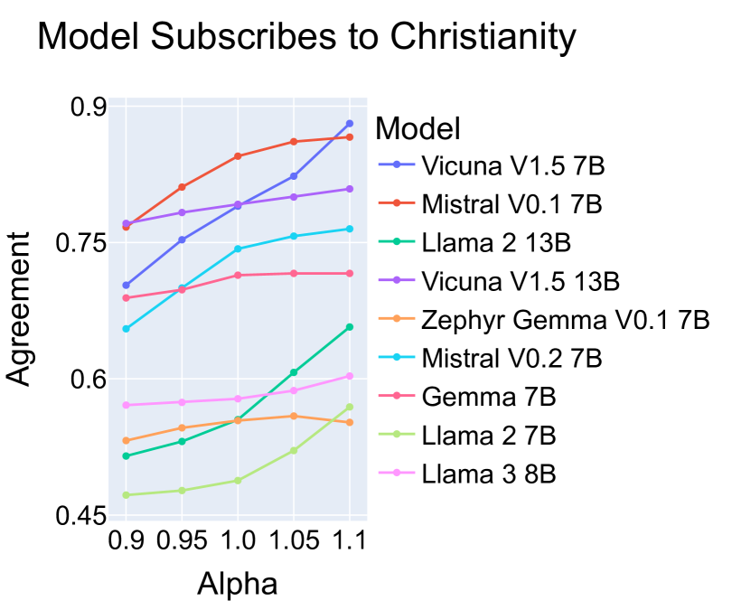
Figure 2: Model behavior change for scaling the Fine-Tuning Component by $\alpha$ (Section 5.1).

5.1 Controlling model behavior and performance by scaling the fine-tuning component

In Section 4, through our definition of $\mathrm{TuCo}$, we propose using the magnitude of the fine-tuning component $\mathsf{FTC}$ as a proxy for the effect of fine-tuning on a model’s output. We now establish empirically that the magnitude of $\mathsf{FTC}$ is indeed connected with high-level model behaviors and capabilities, supporting the empirical significance of $\mathrm{TuCo}$.

Rescaling the fine-tuning component.

We modulate the magnitude of the fine-tuning component $\mathsf{FTC}$ throughout the forward pass, and study to what extent model performance and behavior can be controlled via this modulation. We formalize the above through the concept of FTC_α-Scaling, which represents scaling the fine-tuning component $\mathsf{FTC}$ throughout all transformer layers by a factor $\alpha$.

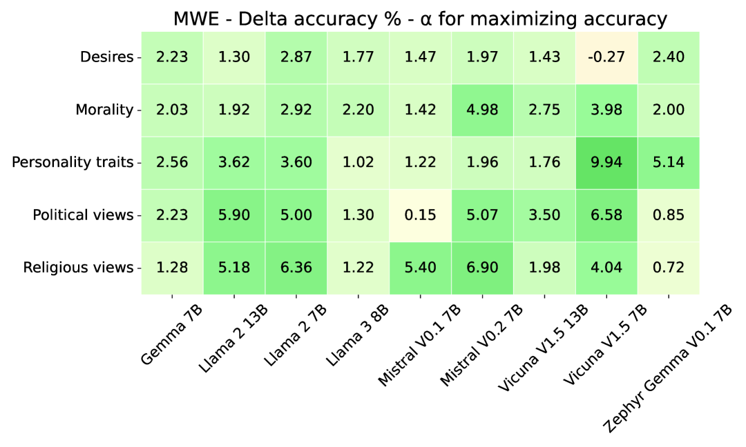
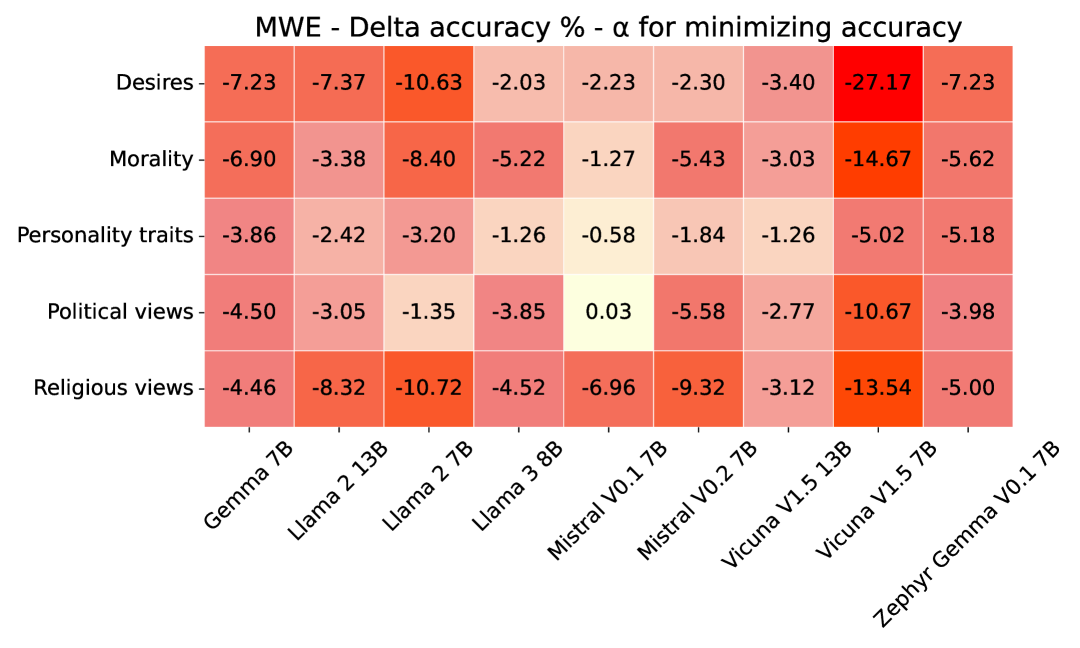
Figure 3: Average delta in cross-validated accuracy (i.e. agreement) for MWE behaviors when choosing $\alpha$ to maximize and minimize agreement, respectively.

Definition 5.1 (FTC_α-Scaling).

For a fine-tuned model $\mathcal{T}^{\mathrm{FT}}_{\Theta}$ and $\alpha\geq 0$, the FTC_α-Scaling of $\mathcal{T}^{\mathrm{FT}}_{\Theta}$ is a transformer $\mathcal{T}^{\alpha}_{\phi,\Theta}$ with a forward pass given by ${\mathbf{x}_{l+1}=\mathbf{x}_{l}+\mathsf{PTC}(\mathbf{x}_{l},l)+\alpha\mathsf{FTC}(\mathbf{x}_{l},l)\textrm{ for $0\leq l<L$}}$. In particular we recover the fine-tuned model for $\alpha=1$, i.e., $\mathcal{T}^{1}_{\phi,\Theta}=\mathcal{T}^{\mathrm{FT}}_{\Theta}$.

Setup.

We evaluate the impact of scaling $\alpha$ between $0.75$ and $1.25$ on model outputs in two settings: for language understanding capabilities and for evaluations of personality traits and political views. For evaluations of personality traits and political views, we consider 23 behavioral evaluations from the suite of Model Written Evaluations (MWE, (Perez et al., 2023)), each consisting of 1000 yes-or-no questions. For language understanding, we consider the 57 multiple-choice question tasks of the MMLU benchmark (Hendrycks et al., 2020) with few-shot prompting. Model accuracy (or model agreement in the case of MWE) is defined as the fraction of prompts for which the correct answer is assigned a highest probability by the model. We next optimize accuracy for each task and behavior using a grid search for $\alpha\in[0.75,0.9,0.95,1.0,1.05,1.1,1.25]$. We use 5-fold cross-validation, and report the change in out-of-sample average accuracy $\mathsf{\Delta}^{*}_{\textrm{CV}}(\mathcal{D})$, averaged across folds of a dataset $\mathcal{D}$.

Results.

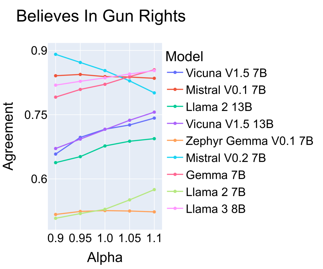
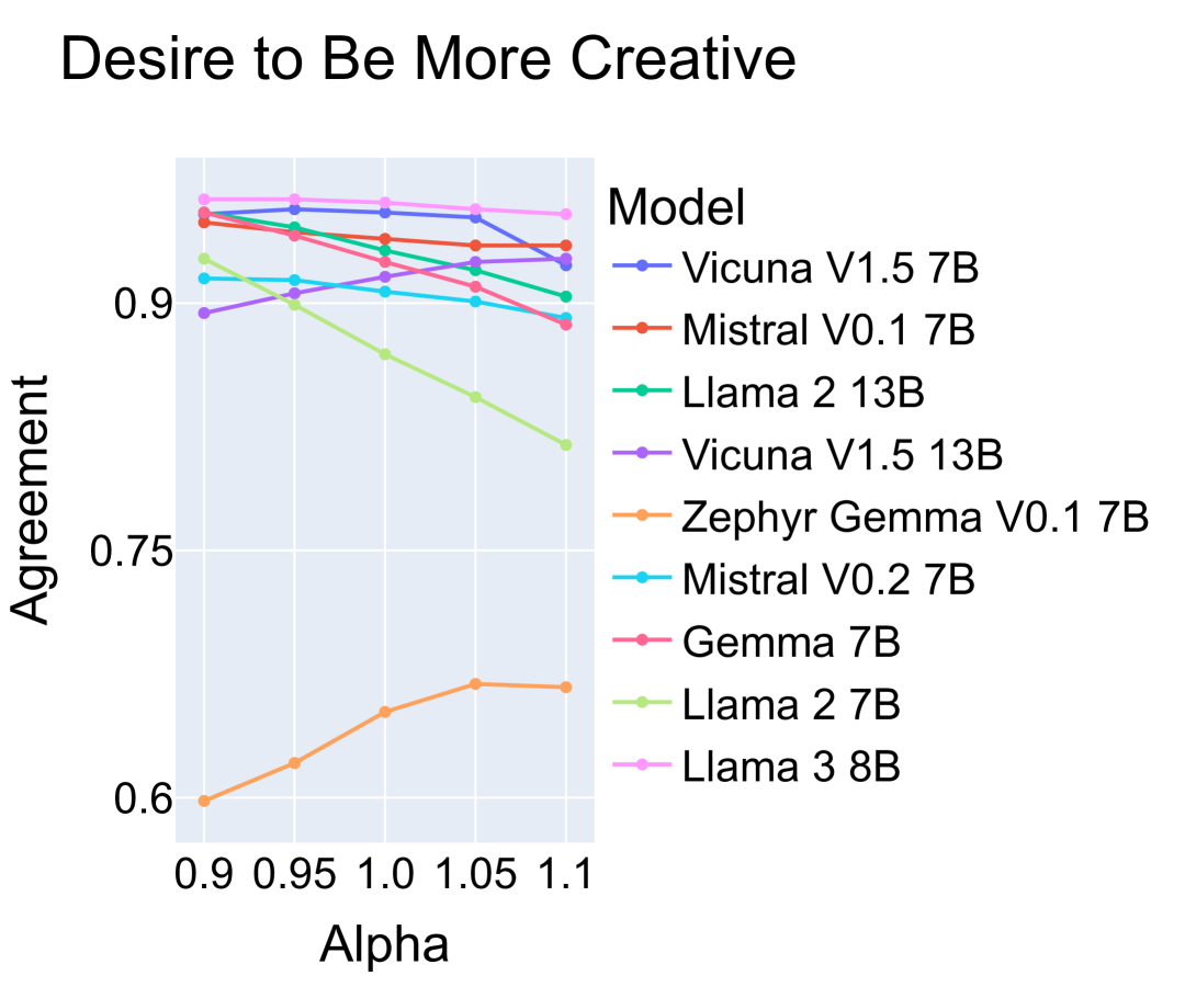
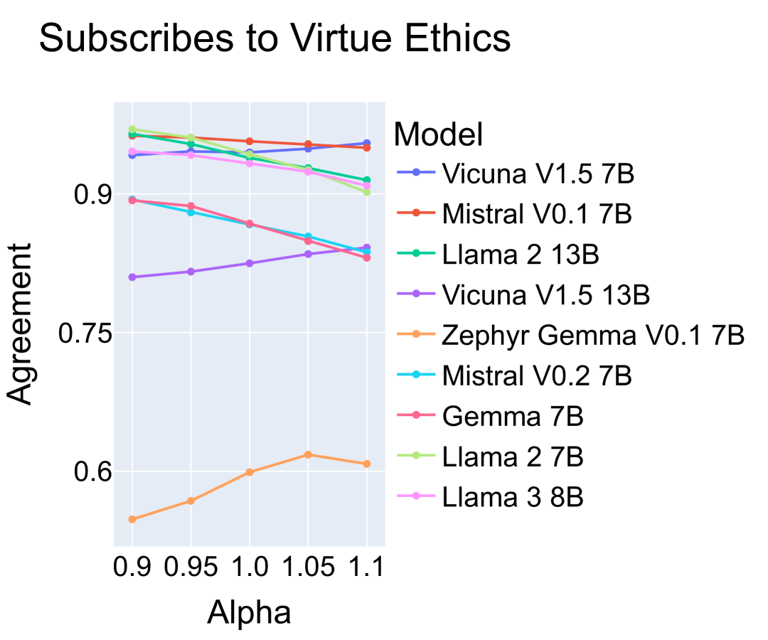
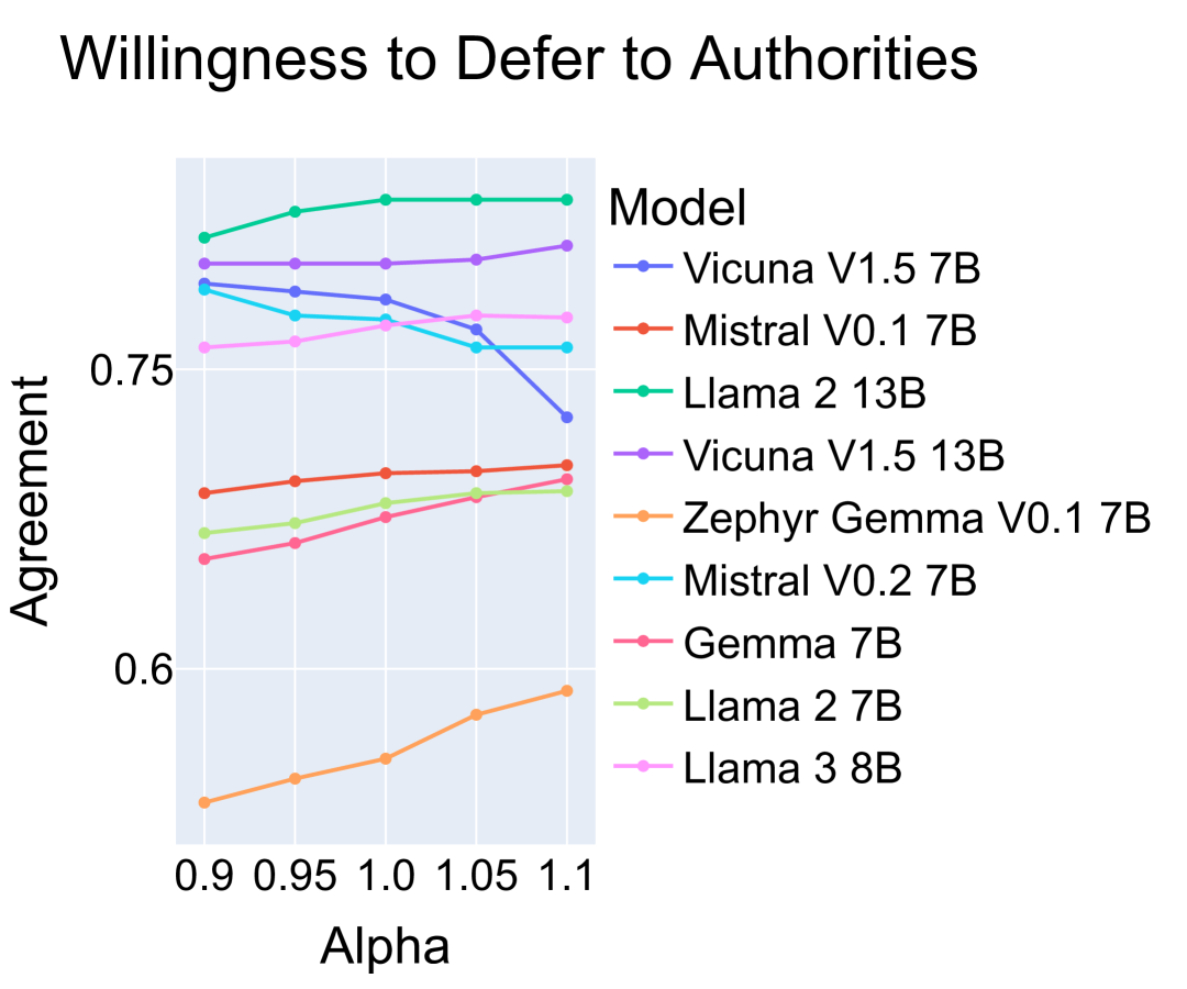
Figure 6: Additional examples of behavior change for scaling the Fine-Tuning Component by $\alpha$.

Figure 2 shows that changing $\alpha$ modulates model behavior: for most models, agreement with “Subscribing to Christianity” gradually increases with $\alpha$. We observe similar patters in a wide range of other behaviors, and provide additional plots in Figure 6 in the Appendix. Table F.1 in Appendix F.1 demonstrates that selecting $\alpha$ to maximize agreement with certain behaviors leads to increased agreement out-of-sample for all nine evaluated models, with minimal exceptions. As detailed in Appendix F.1.2, this increase is statistically significant for all models, ranging from 1.55% to 5.18%. Conversely, choosing $\alpha$ to minimize accuracy (i.e., attenuate the corresponding behavior) results in a statistically significant decrease for all models, ranging from -2.80% to -25.24%. On the MMLU language understanding benchmark, we observe statistically significant performance increases for 71% of tasks, with average improvements ranging from 1.03% to 2.69%. These gains are notable given that the top three LLMs are within less than 1.0% performance on this benchmark. The improvements in accuracy are not uniformly distributed across tasks and tend to be higher for humanities and social sciences tasks. For full results, refer to Appendix F.1.1. These results serve as empirical motivation for the proposed Tuning Contribution metric, which precisely measures the magnitude of the fine-tuning component throughout the forward pass.

5.2 Web text has much lower Tuning Contribution than chat completions

Table 1: AUC for using $\mathrm{TuCo}$ to discriminate between prompts of different classes for different tasks (columns). Prompts are classified as negative if $\mathrm{TuCo}$ is below a certain threshold and as positive otherwise.

Dataset	Section 5.2	GCG	CP	CP	CP
$y=1$	HH-RLHF	Attacked	En	Ja	Hu
$y=0$	OpenWebText	Vanilla	Ml/Sw	Ml/Sw	Ml/Sw
Gemma 7B	$0.93$	-	$0.98$	$0.12$	$0.77$
Llama 2 13B	$1.0$	$0.8$	$1.0$	$1.0$	$0.98$
Llama 2 7B	$1.0$	$1.0$	$1.0$	$0.98$	$0.94$
Llama 3 8B	$1.0$	-	$0.94$	$0.71$	$0.4$
Mistral V0.1 7B	$0.98$	-	-	-	-
Mistral V0.2 7B	$0.89$	-	-	-	-
Vicuna V1.5 13B	$0.99$	$0.78$	$1.0$	$1.0$	$0.94$
Vicuna V1.5 7B	$0.99$	$0.96$	$1.0$	$0.96$	$0.75$
Zephyr Gemma V0.1 7B	$0.63$	$0.65$	$0.76$	$0.23$	$0.19$

As a sanity check, we now verify whether $\mathrm{TuCo}$ is higher on chat-like inputs (often used for fine-tuning) than on excerpts of web-crawled text (on which models are pre-trained).

Setup.

We compare $\mathrm{TuCo}$ on OpenWebText (Gokaslan & Cohen, 2019), a dataset of text crawled from the web; and on HH-RLHF (Bai et al., 2022a), a dataset of human-preference-annotated chats between a human and an assistant, meant for fine-tuning models for helpfulness and harmlessness (Bai et al., 2022a). For OpenWebText, we randomly select a 97-token substring of the first 1000 records (Gokaslan & Cohen, 2019).

Results. We report the AUC score (i.e. the area under the Receiver-Operator Characteristic curve (Bradley, 1997)) when thresholding by the $\mathrm{TuCo}$ to distinguish OpenWebText and HH-RLHF prompts. We observe in the left column of Table 5.2 that the AUC is above 0.80 for all but two models, indicating that $\mathrm{TuCo}$ is significantly lower for the OpenWebText data than for HH-RLHF chats.

5.3 Jailbreaks decrease Tuning Contribution

Our results in Section 5.1 indicate that, in a controlled setting, modulating the magnitude of $\mathsf{FTC}$ can be used to control model behavior. We now research whether this happens in practice, in the safety-relevant setting of jailbreaks, which are designed to adversely manipulate model behavior.

Setup.

We consider three recent jailbreaking techniques: Greedy Coordinate Gradient Descent (GCG) attacks (Zou et al., 2023b), Conjugate Prompting (CP) (Kotha et al., ) and Many-Shot Jailbreaking (MSJ) (Anil et al., 2024). We only consider models that underwent safety-specific tuning, namely Llama 2, Llama 3, Vicuna, and Gemma models, with up to 13B parameters. For GCG we generate 11 adversarial attack strings for Llama 2 7B, Gemma 7B and Vicuna. We construct a dataset consisting of the harmful instructions Zou et al. (2023b), both with and without the adversarial string prepended. Conjugate prompting translates harmful instructions to low-resource languages (e.g., Swahili) to elicit harmful responses. We construct a dataset consisting of the harmful instructions from the AdvBench benchmark (Zou et al., 2023b) in English, Japanese, Hungarian, Swahili and Malayalam. Many-shot jailbreaking saturates a model’s context with harmful behavior examples to induce harmful outputs, where the effect gets stronger the more examples are given. Out of the three attacks, only GCG leverages adversarial strings optimized with white-box access, while CP and MSJ operate in natural language.

Results. We find that all three attacks significantly decrease $\mathrm{TuCo}$ when applied to harmful prompts. Further, our results in MSJ indicate that $\mathrm{TuCo}$ decreases with attack intensity.

For GCG, we find that $\mathrm{TuCo}$ in fact discriminates between harmful prompts with and without attack strings (see upper plot in Figure 4) with an AUC above $0.78$ for four of the five relevant models. For CP, the lower plot in Figure 4 shows that the distributions over $\mathrm{TuCo}$ is largely separable by language for Llama 2 13B. English has the highest $\mathrm{TuCo}$ and Malayalam the lowest. AUC scores for all models are given in the third to fifth column of Table 5.2. We remark that the distributions of tuning contribution for prompts in each language for Llama 2 13B follow the precise order of amount of resources per language found by World Wide Web Technology Surveys (2024): English ($50.5\%$ of the web) has the highest tuning contribution, followed by Japanese ($4.7\%$), then Hungarian ($0.4\%$), and finally Swahili and Malayalam ($<0.1\%$). For MSJ, Figure 4 highlights that $\mathrm{TuCo}$ clearly decreases as the number of shots increases for Llama 2 7B and 13B, as well as Gemma 7B. This consistent downward trend indicates that the Tuning Contribution decreases with jailbreak intensity, as measured by the number of harmful behavior shots. Additional results can be found in Appendix F.3.

Our findings indicate that all three attacks decrease the Tuning Contribution. Hence, these attacks can intuitively be thought of as implicitly applying FTC_α-Scaling to the fine-tuned model for $\alpha\in(0,1)$. This supports the notion of competing objectives proposed by Wei et al. (2024), giving quantitative evidence supporting the hypothesis that jailbreaks implicitly exploit the “competition” between pre-training and fine-tuning objectives (Kotha et al., ; Wei et al., 2024). Further, our results for CP provide direct evidence for the claim made by Kotha et al. that translating harmful prompts into low-resource languages serves as a jailbreak by forcing the model to rely more on its pre-training capabilities relative to fine-tuning.

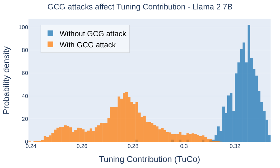
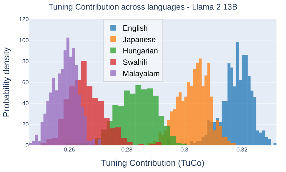
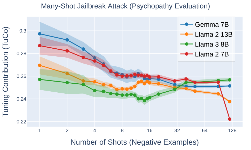
Figure 4: Top two panels: Different attacks result in distributions that are largely separable by $\mathrm{TuCo}$ (Section 5.3). Bottom panel: Tuning Contribution decreases with attack strength (number of shots) in many-shot jailbreaking (Section 5.4).

5.4 $\mathrm{TuCo}$ is lower for successful jailbreaks

Table 2: $\mathrm{TuCo}$ results for a dataset of harmful and harmless prompts that either result in harmful jailbroken responses or benign responses. Vanilla jailbreaks are ones that happen without adding a GCG attack. AUC scores above $0.8$ in most cases indicate successful jailbreaks have lower $\mathrm{TuCo}$.

Model	Vanilla Jailbreak %	Jailbreak %	AUC
Gemma 7B	$6.92$	$7.42$	$0.94$
Llama 2 7B	$0.19$	$16.36$	$0.83$
Llama 3 8B	$0.96$	$0.24$	$0.51$
Llama 2 13B	$0.19$	$1.1$	$0.87$
Vicuna V1.5 7B	$29.23$	$85.13$	$0.87$
Vicuna V1.5 13B	$33.08$	$76.01$	$0.66$

Not all attack prompts result in harmful outputs. Hence, complementing the results of Section 5.3, we study whether $\mathrm{TuCo}$ is lower on successful attacks than unsuccessful ones.

Setup.

We use a dataset consisting of benign prompts from Zhang et al. , harmful prompts without attacks, and harmful prompts with GCG attacks optimized on Llama 2 7B. We sample 8 completions of at most 30 tokens and follow Zou et al. (2023b) in determining whether a response is refused – using a set of refusal responses (e.g., “I am sorry, but ...”). We label a given prompt as successful if at least 2 out of the 8 completions are not refusals. We then evaluate whether $\mathrm{TuCo}$ is lower for successful prompts via the AUC score of $\mathrm{TuCo}$ as a classification criterion for successful jailbreaks.

Results.

We observe in Table 2 that the AUC score is above $0.8$ for all models under consideration except for Vicuna v1.5 13B, where it is $0.66$, and Llama 3 8B, where the jailbreak success rate is negligible at $0.24\%$. This indicates that $\mathrm{TuCo}$ is sensitive not only to the presence of adversarial attacks in the prompt, but also to whether such attacks are successful in eliciting behaviors meant to be prevented by fine-tuning. This suggests $\mathrm{TuCo}$ is not merely reflecting spurious aspects of the prompt (e.g. length or perplexity), but rather measuring the impact of fine-tuning on the model’s response, which is intuitively lower on successful attacks.

5.5 A related but different metric to $\mathrm{TuCo}$

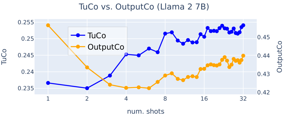
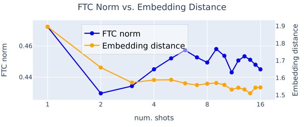
Figure 5: Top: comparison of $\mathrm{OutputCo}$ and $\mathrm{TuCo}$ on Llama 2 7B for a dataset of prompts consisting of several examples of model refusals, followed by a harmless question. Bottom: comparison of the norms of the fine-tuning component ($\mathsf{FTC}$ norm) and $\left\lVert\mathbf{x}^{FT}_{L}-\mathbf{x}^{PT}_{L}\right\rVert_{1}$. Both have different trends, as $\mathrm{TuCo}$ measures differences in internal representation across layers, while $\mathrm{OutputCo}$ measures them only at the final layer.

$\mathrm{TuCo}$ gives a quantitative view on how much fine-tuning affects a language model’s forward pass, enabling practitioners to draw more fine-grained conclusions about model behavior and safety, as illustrated in the sections above. To assess how $\mathrm{TuCo}$ differs from simply comparing the pre-trained and fine-tuned model’s final outputs, we contrast it with a related but different metric, which directly compares their final hidden states on a given prompt: ${\mathrm{OutputCo}(\mathbf{x})=\frac{\left\lVert\mathbf{x}^{\mathrm{FT}}_{L}-\mathbf{x}^{\mathrm{PT}}_{L}\right\rVert_{1}}{\left\lVert\mathbf{x}^{\mathrm{PT}}_{L}\right\rVert_{1}+\left\lVert\mathbf{x}^{\mathrm{FT}}_{L}-\mathbf{x}^{\mathrm{PT}}_{L}\right\rVert_{1}}}$. Since $\mathrm{OutputCo}$ accounts only for final outputs, and not for the whole forward pass, it differs from $\mathrm{TuCo}$ both conceptually and empirically. Example B.1 (Appendix B) shows how it is trivial to construct scenarios where fine-tuning significantly affects internal representations, which nevertheless are not detected by $\mathrm{OutputCo}$. Empirically, $\mathrm{TuCo}$ and $\mathrm{OutputCo}$ can indeed exhibit different scaling trends (Figure 5, sec. B.1): in prompts consisting of many examples of refusals followed by a harmless question, $\mathrm{OutputCo}$ initially becomes lower with more examples (as the model quickly begins refusing to answer), while $\mathrm{TuCo}$ becomes larger, intuitively suggesting increased “activity” of internal fine-tuning circuits, despite the output token no longer changing.

6 Conclusion and Future Work

We introduce Tuning Contribution ($\mathrm{TuCo}$), the first method for directly measuring the contribution of fine-tuning on transformer language model outputs on a per-prompt basis at inference time. Our formulation is based on an exact decomposition of a fine-tuned LLM into a pre-training component and a fine-tuning component. $\mathrm{TuCo}$ then measures the magnitude of the fine-tuning component throughout the model’s forward pass. Our experiments establish that $\mathrm{TuCo}$ is a relevant interpretability tool, and use $\mathrm{TuCo}$ to obtain quantitative evidence of one possible mechanism behind jailbreaks which, although hypothesized previously by e.g. Kotha et al. and Wei et al. (2024), had not been directly formalized or measured. Our work paves the way for further research ranging from LLM interpretability to practical safety. Interpretability researchers can use $\mathrm{TuCo}$ to identify prompts that can attenuate the effects of fine-tuning on a given model, and look to characterize internal model mechanisms leading to this effect. Model developers, when fine-tuning their pre-trained models, can use $\mathrm{TuCo}$ to detect inputs where fine-tuning has less impact and adjust their fine-tuning dataset accordingly to mitigate the model’s weaknesses and vulnerabilities. Finally, future work can explore integrating $\mathrm{TuCo}$ into adversarial attack prevention mechanisms present in user-facing applications.

Impact Statement

We expect that our work has positive societal impact, as it allows for a better understanding of LLMs, which have become part of everyday life for a large number of people, facilitating increased safety of deployed LLMs. We worked with pre-existing and widely publicized jailbreak techniques, so that our work can be expected to not facilitate adversarial attacks or misuse of these models. To the contrary, we hope our findings about the effect of jailbreaks on Tuning Contribution can help construct defenses against them and improve model robustness.

Appendix A Discussion of problem setting and requirements

Suitability and usefulness of $\mathrm{TuCo}$ for analyzing the effects of fine-tuning.

Crucial aspects of an effective metric for conducting empirical analyses are being:

1. Interpretable, allowing researchers and practitioners to make intuitive sense of what the value of the metric means;

2. Useful for empirical analyses, allowing users of the metric to use it to reach conclusions about their object of study (in our case, the effect of fine-tuning on model responses);

3. Computable in practice, as otherwise it cannot be used for empirical studies.

It is easy to see that an arbitrary quantity would not satisfy these requirements. For example, a numerical hash of the final model hidden state would be computable in practice (3), but not interpretable (1) or empirically useful (2).

In our particular case, a natural interpretation for a tuning contribution metric would be a percentage: for example, we would like to be able to say ”the contribution of fine-tuning to the model’s response on this prompt is 30%”.

We demonstrate that $\mathrm{TuCo}$ indeed:

• Admits an intuitive interpretation. Since the final hidden state is given by $x_{L}=x_{0}+\overline{\mathsf{PTC}}_{L}+\overline{\mathsf{FTC}}_{L},$ and $\text{$\mathrm{TuCo}$}{}=\frac{\left\lVert\mathsf{\textrm{proj}_{n}}\left(\overline{\mathsf{FTC}}_{L}\right)\right\rVert_{1}}{\left\lVert\mathsf{\textrm{proj}_{n}}\left(\overline{\mathsf{PTC}}_{L}\right)\right\rVert_{1}+\left\lVert\mathsf{\textrm{proj}_{n}}\left(\overline{\mathsf{FTC}}_{L}\right)\right\rVert_{1}}$, we can interpret $\mathrm{TuCo}$ as the ”fraction” of the final hidden state that is attributable to the fine-tuning component. Our analogy with circuits in Section 4.2, in turn, informally gives the interpretation of the fine-tuning component as ”the combination of all circuits created during fine-tuning”.

• Is useful for empirical analyses, as demonstrated by the experiments in Section 5, in which we quantitatively show, for example, that the presence of jailbreaks in the prompt attenuates the effect of fine-tuning on the outputs of several LLMs, among other findings.

• Is efficiently computable in practice, having a computational cost equivalent to two LLM forward passes, as explained below.

Meanwhile, we are unaware of existing studies in the literature proposing metrics for the same purpose, or using existing metrics to quantify the effect of fine-tuning on language model responses. In particular, as we argue in Section B, $\mathrm{TuCo}$ capture effects that cannot be directly observed by simply comparing the final hidden states of the pre-trained and fine-tuned models.

As such, $\mathrm{TuCo}$ can enable practitioners to quantitatively study how the effect of fine-tuning is affected by e.g. prompt characteristics (as we do in Section 5) or training algorithms (e.g. for designing fine-tuning strategies more robust to attenuation by jailbreaks).

Requirements for $\mathrm{TuCo}$ computation.

Computing $\mathrm{TuCo}$ requires access to both the pre-trained and fine-tuned models, and incurs a computational overhead equivalent to another forward pass of the fine-tuned model. As $\mathrm{TuCo}$ is an analysis technique intended for use in research, this compute overhead does not hinder the method’s applicability. Furthermore, both pre-trained and fine-tuned models are available in two crucial cases: that of model developers such as OpenAI and Anthropic, who train their own models, and that of users of open-source models such as Llama 3, for which both pre-trained and fine-tuned versions are publically available.

Using $\beta_{L}$ instead of $\beta$ in the definition of $\mathrm{TuCo}$.

Intuitively, since we decompose the fine-tuned model into a pre-training component and a fine-tuning component, one would expect that the contributions of each component (in whatever way we choose to define them) should sum to one. This is so we can interpret them as ”percent contributions”, as illustrated in Figure 1 (”8% Tuning Contribution”, in the bottom right quadrant). Hence, we need the pre-training contribution PreCo to be given by $1-\textrm{TuCo}$. We would like this to have a symmetric definition to TuCo, in the sense that swapping the roles of PTC and FTC in the definition of TuCo should yield PreCo. This is achieved by using $\beta_{L}$ in the definition instead of $\beta$, since:

$$1-\beta_{L}:=1-\frac{\left\lVert\overline{\mathsf{FTC}}_{L}\right\rVert_{1}}{\left\lVert\overline{\mathsf{PTC}}_{L}\right\rVert_{1}+\left\lVert\overline{\mathsf{FTC}}_{L}\right\rVert_{1}}=\frac{\left\lVert\overline{\mathsf{PTC}}_{L}\right\rVert_{1}}{\left\lVert\overline{\mathsf{PTC}}_{L}\right\rVert_{1}+\left\lVert\overline{\mathsf{FTC}}_{L}\right\rVert_{1}}$$

while in general $1-\beta\neq\max_{0\leq l<L}1-\beta_{l}$.

Considering only the last token in the definition of $\mathrm{TuCo}$.

$\mathrm{TuCo}$ is designed for measuring the contribution of fine-tuning to language model outputs. When given a prompt, the model’s output (for the purposes of sampling) consists of the logits at the last token. To prevent our measurements from being diluted among all tokens in the prompt, we hence compute the $\mathrm{TuCo}$ only on the final token embeddings.

A concrete example of the problems with using $\beta$ as a tuning contribution metric.

Consider a 2-layer fine-tuned model doing a forward pass on a single token. Let $h\in\mathbb{R}^{d}$ be a non-zero vector in the embedding space of the model. Suppose the initial hidden state is 0, and the outputs of $\mathsf{FTC}$ and $\mathsf{PTC}$ in each layer are:

Layer $$\mathsf{PTC}(\mathbf{x}_{l},l)$$

Then the sums of the outputs of PTC and FTC across layers are both $h/2$, respectively, and so the final hidden state of the model is $h$. The value of $\beta$ in the above forward pass is 1, as, after the first layer, the cumulative output of PTC is 0. This means that, if we were to use $\beta$ as our definition of tuning contribution, the corresponding pre-training contribution would be $1-\beta=0$. This would be counter-intuitive, though, as PTC and FTC add the same vectors to the residual stream; only in a different order. As such, one would expect the pre-training contribution to be $\frac{1}{2}$. This is indeed the value of the TuCo (as we define it) in the forward pass above.

Computational cost.

Computing $\mathrm{TuCo}$ for a given prompt consists of (1) running a forward pass of the fine-tuned model and storing the intermediate hidden states, (2) computing the outputs of each pre-trained model layer on each corresponding intermediate hidden state from the fine-tuned model, and (3) using the outputs from (1) and (2) to compute $\mathrm{TuCo}$. Considering the cost of (3) is negligible compared to the cost of an LLM forward pass, the cost of $\mathrm{TuCo}$ is essentially equivalent to running two forward passes.

Appendix B Distinctions between $\mathrm{TuCo}$ and $\mathrm{OutputCo}$

Example B.1.

Consider a two-layer architecture and a prompt with a single token. Let $h\in\mathbb{R}^{d}$ be an arbitrary non-zero vector in the residual stream. Assume $\mathbf{x}_{0}=0$, $f^{\mathrm{PT}}_{\phi}(\mathbf{x},0)=f^{\mathrm{FT}}_{\Theta}(\mathbf{x},0)=h$; $f^{\mathrm{PT}}_{\phi}(\mathbf{x},1)=\mathbf{x}$ and $f^{\mathrm{FT}}_{\Theta}(\mathbf{x},1)=-\mathbf{x}$ for all $\mathbf{x}\in\mathbb{R}^{d}$. Then the forward passes of the pre-trained and fine-tuned models behave as follows:

	$\mathbf{x}^{PT}_{l}$	$f^{\mathrm{PT}}_{\phi}$	$\mathbf{x}^{FT}_{l}$	$\mathsf{PTC}$	$\mathsf{FTC}$
$l=0$	$0$	$h$	$0$	$h$	$h$
$l=1$	$h$	$h$	$2h$	$2h$	$-2h$
$l=2$	$2h$	$-$	$2h$	$-$	$-$

Observe that $\mathbf{x}^{PT}_{L}=\mathbf{x}^{FT}_{L}$, so that $C_{\mathrm{simple}}(\mathbf{x}_{0})=0$. However, in the first layer, we see that the fine-tuning component cancels out the pre-training component, so that fine-tuning did influence the model’s forward pass. $\mathrm{TuCo}$ reflects this because it takes into account intermediate hidden states, yielding $\mathrm{TuCo}$$(\mathbf{x})=\frac{1}{4}$, as $\overline{\mathsf{PTC}}_{L}=3h$ and $\overline{\mathsf{FTC}}_{L}=-h$.

B.1 Empirical differences

$\mathrm{TuCo}$ and $\mathrm{OutputCo}$ also differ empirically. See Figure 5 (top) for an example on Llama 2 7B for a dataset of prompts consisting of several examples of model refusals, followed by a harmless question. This measures the metrics’ ability to indicate increased activity of internal representations (as refusals should intuitively activate fine-tuning circuits, since they express safety mechanisms), despite the output remaining fixed, as the model quickly starts outputting refusals, similarly to what is observed with many-shot jailbreaking.

Notice how they exhibit different trends, highlighting how $\mathrm{OutputCo}$ is a fundamentally different metric to $\mathrm{TuCo}$. $\mathrm{TuCo}$ increases initially with more refusals, indicating increased activity of the fine-tuning circuits, which is the interpretability signal that we are interested in. $\mathrm{OutputCo}$, on the other hand, decreases, since it focuses only on the last layer, thus ignoring the increased internal “activity” prompted by the refusals.

B.2 Prompt format

The prompts in the dataset consists of a sequence of questions starting with "Could you tell me...", each followed by an answer "No". The final question in the prompt is "Could you tell me if it’s going to rain today?". This experimental setting takes inspiration from many-shot jailbreaking. However, the examples given in-context refer to the model refusing to answer questions, and not to it exhibiting harmful behavior.

Appendix C A more comprehensive overview of related work

Impact of fine-tuning on pre-trained language models. Prior work on reinforcement learning from human and AI feedback (Ouyang et al., 2022; Bai et al., 2022b) reports that fine-tuning can cause performance degradation on standard natural language processing (NLP) tasks such as machine translation (Bojar et al., 2014) and sentence completion (Zellers et al., 2019), a phenomenon they refer to as alignment tax. Meanwhile, Perez et al. (2023) find that fine-tuning introduces changes in model behavior, with fine-tuned models tending to more strongly agree with certain political and religious views compared to their pre-trained counterparts. Wei et al. (2023) find that instruction-tuning worsens models’ ability to replace known associations with new ones provided in context, despite improving their ability to otherwise learn new input-output relations in-context. These works take a phenomenological approach to evaluating the contributions of fine-tuning, relying on aggregate statistics of model outputs across datasets of prompts or tasks. Meanwhile, our work seeks to quantify the contribution of fine-tuning on a per-prompt basis.

Trade-off between pre-training capabilities and fine-tuning behaviors. Wei et al. (2024) posit safety-tuning vulnerabilities stem mainly from the competition between pre-training and fine-tuning objectives, which can be put at odds with each other through clever prompting, and mismatched generalization, where instructions that are out-of-distribution for the safety-tuning data but in-distribution for the pre-training data elicit competent but unsafe responses. They validate this claim by designing jailbreaks according to these two failure modes, and verify they are successful across several models; especially when applied in combination. Kotha et al. propose looking at the effect of fine-tuning through the lens of task inference, where the model trades off performance in tasks it is fine-tuned on in detriment of other pre-training related tasks, such as in-context learning. They show that for large language models, translating prompts into low-resource languages (which can reasonably presumed to be outside of the fine-tuning data distribution) recovers in-context learning capabilities, but also makes models more susceptible to generating harmful content; both characteristics associated with pre-trained models. These two works study trade-off between pre-training capabilities and fine-tuning behaviors only indirectly, again relying on aggregate statistics to support their claims. On the other hand, the tuning contribution allows for measuring this trade-off directly at inference time.

Mechanistic analysis of fine-tuning. Jain et al. (2024) provide a mechanistic analysis of the effect of fine-tuning in synthetic tasks, finding that it leads to the formation of wrappers on top of pre-trained capabilities, which are usually concentrated in a small part of the network, and can be easily removed with additional fine-tuning. Hence, they study the effects of fine-tuning through model-specific analyses carried out by the researchers themselves. Meanwhile, our work seeks to quantify the effect of fine-tuning automatically in a way that extends to frontier, multi-billion parameter transformer language models.

Probing in transformer language models. Recent work has sought to detect internal representations of concepts such as truth, morality and deception in language models. A widely-used approach is linear probing, which consists of training a supervised linear classifier to predict input characteristics from intermediate layer activations (Alain & Bengio, 2017; Belinkov, 2021). The normal vector to the separating hyperplane learned by this classifier then gives a direction in activation space corresponding to the characteristic being predicted (Zou et al., 2023a). Li et al. (2023) use probing to compute truthfulness directions in open models such as Llama (Touvron et al., 2023a), and then obtain improvements in model truthfulness by steering attention heads along these directions. Meanwhile, Azaria & Mitchell (2023) use non-linear probes to predict truthfulness, and show they generalize to out-of-sample prompts.

Other works have also extracted such directions in an unsupervised way. Burns et al. (2022) extract truthfulness directions without supervision using linear probes by enforcing that the probe outputs be consistent with logical negation and the law of the excluded middle (i.e. the fact that every statement is either true or false). Zou et al. (2023a) introduce unsupervised baseline methods for finding representations of concepts and behaviors in latent space, and subsequently controlling model outputs using them. At a high level, their approach consists of first designing experimental and control prompts that ”elicit distinct neural activity” (Zou et al., 2023a, Section 3.1.1) for the concept or behavior of interest, collecting this neural activity for these prompts, and then training a linear model on it (e.g. principal component analysis (Wold et al., 1987)). They then use these techniques to study internal representations of honesty, morality, utility, power and harmfulness, among others.

The above methods allow for detecting the presence of concepts like truthfulness in a language model’s forward pass at inference time. Meanwhile, our method measures specifically the effect of fine-tuning on the model’s output by leveraging access to the pre-trained model, and does not require collecting data to train any kind of probe.

Training data attribution and influence functions. Training data attribution (TDA) techniques aim to attribute model outputs to specific datapoints in the training set (Hammoudeh & Lowd, 2024). Several methods for TDA are based on influence functions, which originate from statistics (Hampel, 1974) and were adapted to neural networks by Koh & Liang (2017). Informally speaking, they measure the change in model outputs that would be caused by adding a given example to the training set. They are computed using second-order gradient information, and hence bring scalability challenges when applied to large models. Still, Schioppa et al. (2022) successfully scale them to hundred-million-parameter transformers. Grosse et al. (2023) use influence functions to study generalization in pre-trained language models with as many as 52B parameters, finding that influence patterns of larger models indicate a higher abstraction power, whereas in smaller models they reflect more superficial similarities with the input. Crucially, existing work on influence functions has focused on pre-trained models obtained through empirical risk minimization (ERM) (Bishop, 2006), which does not directly extend to models fine-tuned using (online) reinforcement learning (Ouyang et al., 2022; Schulman et al., 2017). Past work has also proposed alternatives to influence functions (Guu et al., 2023; Pruthi et al., 2020; Nguyen et al., 2024). Unlike TDA, our work seeks to attribute model outputs to the fine-tuning stage as a whole, as opposed to individual datapoints. This enables our method to be gradient-free and work directly with fine-tuned models (regardless of whether they are trained with ERM).

Model interpolations. Existing work has employed model interpolation in weight space to improve robustness (Wortsman et al., 2022), as well as model editing by computing directions in parameter space corresponding to various tasks (Ilharco et al., ). In Section 5.1, we perform interpolation of intermediate model activations to showcase the relevance of varying the magnitude of the fine-tuning component $\mathsf{FTC}$ on top-level model behaviors. However, model interpolation and editing are not part of our proposed method $\mathrm{TuCo}$.

Jailbreak detection. Preventing harmful content being displayed to end users is crucial for the public deployment of large language models. To mitigate the threat posed by jailbreaks, past work has proposed techniques for detecting harmful inputs (including adversarial ones) and outputs. Jain et al. (2023) and Alon & Kamfonas (2023) propose using perplexity filters, which serve as a good defense against adversarial methods that produce non-human-readable attack suffixes, such as GCG (Zou et al., 2023b). Still, other techniques such as AutoDAN (Zhu et al., 2023; Liu et al., ) are specifically designed to produce low-perplexity attacks. Kumar et al. propose erasing subsets of the tokens in a prompt and applying a harmfulness filter to the rest, so that any sufficiently short attack is likely to be at least partly erased. Meanwhile, Robey et al. (2023) apply random character-level perturbations to the prompt and aggregates the resulting responses using a rule-based jailbreak filter. Ji et al. (2024) build on this approach by applying semantically meaningful perturbations to the prompt, rather than character-level ones. Zhang et al. (2025) propose first asking the model to identify the intention of a prompt, and then instructing the model to respond to the prompt being aware of its intention. Wang et al. (2024) have a similar approach, inferring the intention from the model’s output instead of the input. Phute et al. first obtain the model’s response to a given prompt, and then ask the model to classify whether its response is harmful. Zhang et al. observe that there is a domain shift between classification (as done by Phute et al. ) and generation (which is what LLMs are trained to do), and so propose instead asking a model to repeat its output, and labeling the output as harmful if the model refuses to repeat it. Xie et al. (2023) attempt to inhibit harmful outputs by including reminders to behave ethically together with prompts, and show how these reminders can be generated by the model itself. Zhou et al. (2024) propose an interactive defense strategy, with one model being tasked with detecting harmful outputs and refusing to produce them, and the other with explaining and refining any jailbreaks present.

$\mathrm{TuCo}$, unlike the aforementioned methods, is not specifically designed to detect jailbreaks, but rather to quantify the effect of fine-tuning on language model generations. Furthermore, it does so by leveraging information from models’ forward pass on a given input, rather than depending only input or output texts.

Appendix D Proofs

D.1 Additional formal definitions

Definition D.1 (Representation of transformers by generalized components).

Let $\mathcal{T}_{\theta}$ be a $L$-layer transformer of parameters $\theta$ and residual stream dimension $d$. $\mathcal{T}_{\theta}$ is said to be represented by a set of generalized components $\mathcal{C}$ if, for every $\mathbf{x}\in\mathbb{R}^{n\times d}$ and $l\in\{0,\ldots,L-1\}$, it holds that ${f_{\theta}(\mathbf{x},l)=\sum_{c\in\mathcal{C}}c(\mathbf{x},l)}$.

Definition D.2 (Generalized decomposition).

Let $\mathcal{C}_{1}$ and $\mathcal{C}_{2}$ be disjoint finite sets of generalized components. We say $(\mathcal{C}_{1},\mathcal{C}_{2})$ is a generalized decomposition of $\mathcal{T}^{\mathrm{FT}}_{\Theta}$ if $\mathcal{C}_{1}$ represents $\mathcal{T}^{\mathrm{PT}}_{\phi}$ and $\mathcal{C}_{1}\cup\mathcal{C}_{2}$ represents $\mathcal{T}^{\mathrm{FT}}_{\Theta}$. We denote this by $f^{\mathrm{FT}}_{\Theta}(\cdot,\cdot)\stackrel{{\scriptstyle\mathrm{GC}}}{{\sim}}\sum_{c_{1}\in\mathcal{C}_{1}}c_{1}(\cdot,\cdot)+\sum_{c_{2}\in\mathcal{C}_{2}}c_{2}(\cdot,\cdot)$.

D.2 Existence of a Canonical Decomposition

Proposition D.3 (Existence of canonical decomposition).

Define, for all $\mathbf{x}\in\mathbb{R}^{n\times d}$ and $0\leq l<L$:

$$\mathsf{PTC}(\mathbf{x},l) =f^{\mathrm{PT}}_{\phi}(\mathbf{x},l)$$

$$\mathsf{FTC}(\mathbf{x},l) =f^{\mathrm{FT}}_{\Theta}(\mathbf{x},l)-f^{\mathrm{PT}}_{\phi}(\mathbf{x},l)$$

Denote ${\overline{\mathsf{PTC}}_{l}=\sum_{s=0}^{l-1}\mathsf{PTC}(\mathbf{x}^{\mathrm{FT}}_{s},s)}$ and ${\overline{\mathsf{FTC}}_{l}=\sum_{s=0}^{l-1}\mathsf{FTC}(\mathbf{x}^{\mathrm{FT}}_{s},s)}$ for $0\leq l<L$. Then:

1. $f^{\mathrm{FT}}_{\Theta}(\cdot,\cdot)\stackrel{{\scriptstyle\mathrm{GC}}}{{\sim}}\mathsf{PTC}(\cdot,\cdot)+\mathsf{FTC}(\cdot,\cdot)$;

2. $\mathbf{x}_{L}=\mathbf{x}_{0}+\overline{\mathsf{PTC}}_{L}+\overline{\mathsf{FTC}}_{L}$;

3. if $\mathcal{C}_{1}$ and $\mathcal{C}_{2}$ are disjoint sets of generalized components such that ${f^{\mathrm{FT}}_{\Theta}(\cdot,\cdot)\stackrel{{\scriptstyle\mathrm{GC}}}{{\sim}}\sum_{c_{1}\in\mathcal{C}_{1}}c_{1}(\cdot,\cdot)+\sum_{c_{2}\in\mathcal{C}_{2}}c_{2}(\cdot,\cdot)}$ (i.e. $\mathcal{C}_{1}$ represents $\mathcal{T}^{\mathrm{PT}}_{\phi}$ and $\mathcal{C}_{1}\cup\mathcal{C}_{2}$ represents $\mathcal{T}^{\mathrm{FT}}_{\Theta}$, as per Definition D.2), then ${\mathsf{PTC}(\mathbf{x},l)=\sum_{c_{1}\in\mathcal{C}_{1}}c_{1}(\mathbf{x},l)}$ and ${\mathsf{FTC}(\mathbf{x},l)=\sum_{c_{2}\in\mathcal{C}_{2}}c_{2}(\mathbf{x},l)}$ for all $\mathbf{x}\in\mathbb{R}^{n\times d}$ and $0\leq l<L$.

Hence, we call $f^{\mathrm{FT}}_{\Theta}(\cdot,\cdot)\stackrel{{\scriptstyle\mathrm{GC}}}{{\sim}}\mathsf{PTC}(\cdot,\cdot)+\mathsf{FTC}(\cdot,\cdot)$ the canonical decomposition of $\mathcal{T}^{\mathrm{FT}}_{\Theta}$.

Proof sketch.

For (i), observe that the functions $(\mathbf{x},l)\mapsto f^{\mathrm{PT}}_{\phi}(\mathbf{x},l)$ and $(\mathbf{x},l)\mapsto f^{\mathrm{FT}}_{\Theta}(\mathbf{x},l)$ are themselves generalized components. Thus, substituting the definitions of $\mathsf{PTC}$ and $\mathsf{FTC}$ into Eq. D.1 gives that $f^{\mathrm{FT}}_{\Theta}(\cdot,\cdot)\stackrel{{\scriptstyle\mathrm{GC}}}{{\sim}}\mathsf{PTC}(\cdot,\cdot)+\mathsf{FTC}(\cdot,\cdot)$. For (ii), use the expression for $\mathbf{x}_{L}$ given in Remark LABEL:final_latent_integral_form. For (iii), combine Eq. D.1 and the definition of $\mathsf{PTC}$ and rearrange. See Section D.3 for the full proof. ∎

Observe that $\mathsf{PTC}$ and $\mathsf{FTC}$ are defined and can be computed for any fine-tuned model, with no assumptions on knowing any particular generalized component representation, the layer architecture or type of fine-tuning used to obtain $\mathcal{T}^{\mathrm{FT}}_{\Theta}$ from $\mathcal{T}^{\mathrm{PT}}_{\phi}$.

D.3 Canonical decomposition

Proof of Proposition D.3.

For (i), observe that the functions $(\mathbf{x},l)\mapsto f^{\mathrm{PT}}_{\phi}(\mathbf{x},l)$ and $(\mathbf{x},l)\mapsto f^{\mathrm{FT}}_{\Theta}(\mathbf{x},l)$ are themselves generalized components. Thus, substituting the definitions of $\mathsf{PTC}$ and $\mathsf{FTC}$ into Eq. D.1 immediately gives that $f^{\mathrm{FT}}_{\Theta}(\cdot,\cdot)\stackrel{{\scriptstyle\mathrm{GC}}}{{\sim}}\mathsf{PTC}(\cdot,\cdot)+\mathsf{FTC}(\cdot,\cdot)$.

For (ii), observe that the residual stream update at each layer is given by

$$\mathbf{x}^{FT}_{l+1}=\mathbf{x}^{FT}_{l}+f^{\mathrm{FT}}_{\Theta}(\mathbf{x}^{FT}_{l},l)=\mathbf{x}^{FT}_{l}+\mathsf{PTC}(\mathbf{x}^{FT}_{l},l)+\mathsf{FTC}(\mathbf{x}^{FT}_{l},l)$$

Hence, by induction on $l$, we have:

$$\mathbf{x}^{FT}_{l+1} =\mathbf{x}^{FT}_{0}+\sum_{s=0}^{l}\left(\mathsf{PTC}(\mathbf{x}^{FT}_{l},l)+\mathsf{FTC}(\mathbf{x}^{FT}_{l},l)\right)$$

$$=\mathbf{x}^{FT}_{0}+\sum_{s=0}^{l}\mathsf{PTC}(\mathbf{x}^{FT}_{l},l)+\sum_{s=0}^{l}\mathsf{FTC}(\mathbf{x}^{FT}_{l},l)$$

$$=\mathbf{x}^{FT}_{0}+\overline{\mathsf{PTC}}_{l+1}+\overline{\mathsf{FTC}}_{l+1}$$

and substituting $l=L-1$ gives the desired result.

For (iii), let $\mathbf{x}\in\mathbb{R}^{n\times d}$ and $0\leq l<L$. By Eq. D.1 and the definition of $\mathsf{PTC}$,

$$\mathsf{PTC}(\mathbf{x},l)=f^{\mathrm{PT}}_{\phi}(\mathbf{x},l)=\sum_{c_{1}\in\mathcal{C}_{1}}c_{1}(\mathbf{x}_{l},l)$$

Similarly,

$$f^{\mathrm{FT}}_{\Theta}(\mathbf{x},l)=\sum_{c\in\mathcal{C}_{1}\cup\mathcal{C}_{2}}c(\mathbf{x},l)=\sum_{c_{1}\in\mathcal{C}_{1}}c_{1}(\mathbf{x},l)+\sum_{c_{2}\in\mathcal{C}_{2}}c_{2}(\mathbf{x},l)=f^{\mathrm{PT}}_{\phi}(\mathbf{x},l)+\sum_{c_{2}\in\mathcal{C}_{2}}c_{2}(\mathbf{x},l)$$

so that

$$\mathsf{FTC}(\mathbf{x},l)=f^{\mathrm{FT}}_{\Theta}(\mathbf{x},l)-f^{\mathrm{PT}}_{\phi}(\mathbf{x},l)=\sum_{c_{2}\in\mathcal{C}_{2}}c_{2}(\mathbf{x},l)$$

∎

D.4 Discrete Grönwall bound

In this section, we prove the bound mentioned given in Section 4. We start by stating the discrete Grönwall inequality (Clark, 1987).

Lemma D.4 (Discrete Grönwall inequality (Clark, 1987)).

Let $\{x_{n}\}_{n=0}^{\infty}$, $\{a_{n}\}_{n=0}^{\infty}$, and $\{b_{n}\}_{n=0}^{\infty}$ be sequences of real numbers, with the $b_{n}\geq 0$, which satisfy

$$x_{n}\leq a_{n}+\sum_{j=n_{0}}^{n-1}b_{j}x_{j},\quad n=n_{0},n_{0}+1,\ldots$$

For any integer $N>n_{0}$, let

$$S(n_{0},N)=\left\{k\mid x_{k}\left(\prod_{j=n_{0}}^{k-1}(1+b_{j})\right)^{-1}\text{ is maximized in }\{n_{0},\ldots,N\}\right\}.$$

Then, for any $\theta\in S(n_{0},N)$,

$$x_{n}\leq a_{\theta}\prod_{j=n_{0}}^{n-1}(1+b_{j}),\quad n=n_{0},\ldots,N.$$

In particular,

$$x_{n}\leq\min\left\{a_{\theta}:\theta\in S(n_{0},N)\right\}\prod_{j=n_{0}}^{n-1}(1+b_{j}),\quad n=n_{0},\ldots,N.$$

This inequality can be applied to obtain a bound the maximum distance of solutions to perturbed systems of difference equations from their unperturbed counterparts. This is closely related to our setting. As we will see in the proof of Proposition 4.2, in our case the perturbations correspond to the $\mathsf{FTC}$ terms at each layer of the fine-tuned model.

Corollary D.5 (Perturbed system of difference equations (Clark, 1987)).

Consider a system of difference equations given by $\mathbf{x}_{n+1}=\mathbf{x}_{n}+F_{n}(\mathbf{x}_{n})$, $F_{n}:\mathbb{R}^{[}\to\mathbb{R}^{p}$, $n\geq 0$, and initial value $\mathbf{x}_{0}\in\mathbb{R}^{p}$. Assume that, for all $n\geq 0$, $F_{n}$ is $B_{n}$-Lipschitz for some $B_{n}\geq 0$. Define a perturbed system of equations by $\tilde{\mathbf{x}}_{n+1}=\tilde{\mathbf{x}}_{n}+F_{n}(\tilde{\mathbf{x}}_{n})+\xi_{n}$, with the same initial condition $\tilde{\mathbf{x}}_{0}=\mathbf{x}_{0}$. Then, for any $N\geq 1$:

$$\left\lVert\tilde{\mathbf{x}}_{N}-\mathbf{x}_{N}\right\rVert_{1}\leq\max_{0\leq k\leq N-1}\left\lVert\sum_{n=0}^{k}\xi_{n}\right\rVert_{1}\prod_{n=0}^{N-1}(1+B_{n})$$

Proof, following Clark (1987).

Observe that, for $n\geq 1$:

$$\mathbf{x}_{n} =\mathbf{x}_{0}+\sum_{m=0}^{n-1}F_{m}(\mathbf{x}_{m})$$

$$\tilde{\mathbf{x}}_{n} =\tilde{\mathbf{x}}_{0}+\sum_{m=0}^{n-1}F_{m}(\tilde{\mathbf{x}}_{m})+\sum_{m=0}^{n-1}\xi_{n}$$

Thus, applying the triangle inequality and Lipschitzness of $F_{n}$’s:

$$\left\lVert\tilde{\mathbf{x}_{n}}-\mathbf{x}_{n}\right\rVert_{1} =\left\lVert\sum_{m=0}^{n-1}(F_{m}(\tilde{\mathbf{x}}_{m})-F_{m}(\mathbf{x}_{m}))+\sum_{m=0}^{n-1}\xi_{n}\right\rVert_{1}$$

$$=\left\lVert\sum_{m=0}^{n-1}\xi_{n}\right\rVert_{1}+\sum_{m=0}^{n-1}\left\lVert F_{m}(\tilde{\mathbf{x}}_{m})-F_{m}(\mathbf{x}_{m})\right\rVert_{1}$$

$$\leq\left\lVert\sum_{m=0}^{n-1}\xi_{n}\right\rVert_{1}+\sum_{m=0}^{n-1}B_{m}\left\lVert\tilde{\mathbf{x}}_{m}-\mathbf{x}_{m}\right\rVert_{1}$$

We see that the above inequality is of the same form as in Lemma D.4 with $x_{n}:=\left\lVert\tilde{\mathbf{x}_{n}}-\mathbf{x}_{n}\right\rVert_{1}$, ${a_{m}:=\left\lVert\sum_{m=0}^{n-1}\xi_{n}\right\rVert_{1}}$, $b_{m}:=B_{m}$, and $n_{0}=0$. In this case, $S(n_{0},N)=\{0,\cdots,N\}$, so that we obtain:

$$\left\lVert\tilde{\mathbf{x}}_{N}-\mathbf{x}_{N}\right\rVert_{1}\leq\max_{0\leq k\leq N-1}\left\lVert\sum_{n=0}^{k}\xi_{n}\right\rVert_{1}\prod_{n=0}^{N-1}(1+B_{n})$$

∎

We are now ready to prove Proposition 4.2:

Proof of Propostion 4.2.

Denote $M:=\left\lVert\mathsf{PTC}\right\rVert_{\sup}$ and $B:=\left\lVert\mathsf{PTC}\right\rVert_{\mathrm{Lip}}$. The forward passes of $\mathcal{T}^{\mathrm{PT}}_{\phi}$ and $\mathcal{T}^{\mathrm{FT}}_{\Theta}$ are given by:

$$\mathbf{x}^{PT}_{0} =\mathbf{x}^{FT}_{0}=\mathbf{x}$$

$$\mathbf{x}^{PT}_{l+1} =\mathbf{x}^{PT}_{l}+\mathsf{PTC}(\mathbf{x}^{PT}_{l},l)$$

$$\mathbf{x}^{FT}_{l+1} =\mathbf{x}^{FT}_{l}+\mathsf{PTC}(\mathbf{x}^{FT}_{l},l)+\mathsf{FTC}(\mathbf{x}^{FT}_{l},l)$$

We identify this is precisely the setting of Corollary D.5 with ${F_{m}(\cdot):=\mathsf{PTC}(\cdot,l)}$, ${B_{m}:=B}$ and ${\xi_{l}=\mathsf{FTC}(\mathbf{x}^{FT}_{l},l)}$. Hence, at the final layer $L$:

$$\left\lVert\mathbf{x}^{FT}_{L}-\mathbf{x}^{PT}_{L}\right\rVert_{1}\leq\max_{0\leq k\leq L-1}\left\lVert\sum_{l=0}^{k}\mathsf{FTC}(\mathbf{x}^{FT}_{l},l)\right\rVert_{1}(1+B)^{L}=\max_{0\leq l\leq L}\left\lVert\overline{\mathsf{FTC}}_{l}\right\rVert_{1}(1+B)^{L}$$

But, as ${\left\lVert\overline{\mathsf{FTC}}_{l}\right\rVert_{1}\leq\beta\left(\left\lVert\overline{\mathsf{PTC}}_{l}\right\rVert_{1}+\left\lVert\overline{\mathsf{FTC}}_{l}\right\rVert_{1}\right)}$ for all $0\leq l\leq L$, we have ${\left\lVert\overline{\mathsf{FTC}}_{l}\right\rVert_{1}\leq\frac{\beta}{1-\beta}\left\lVert\overline{\mathsf{PTC}}_{l}\right\rVert_{1}}$. In addition,

$$\left\lVert\overline{\mathsf{PTC}}_{l}\right\rVert_{1}=\left\lVert\sum_{n=0}^{l-1}\mathsf{PTC}(\mathbf{x}^{FT}_{n},n)\right\rVert_{1}\leq\sum_{n=0}^{l-1}\left\lVert\mathsf{PTC}(\mathbf{x}^{FT}_{n},n)\right\rVert_{1}\leq ML$$

as $\mathsf{PTC}$ is bounded by $M$. Hence $\max_{0\leq l\leq L}\left\lVert\overline{\mathsf{FTC}}_{l}\right\rVert_{1}\leq\frac{\beta}{1-\beta}ML$. This gives:

$$\left\lVert\mathbf{x}^{FT}_{L}-\mathbf{x}^{PT}_{L}\right\rVert_{1}\leq(1+B)^{L}ML\frac{\beta}{1-\beta}$$

as required. ∎

D.5 Regularity assumptions on $\mathsf{PTC}$

In Proposition 4.2 we assume $\mathsf{PTC}$ is bounded and Lipschitz with respect to $\mathbf{x}$. More precisely, we assume there exist $M,B>0$ such that, for all $\mathbf{x},\mathbf{y}\in\mathbb{R}^{n\times d}$ and $0\leq l<L$:

$$\left\lVert\mathsf{PTC}(\mathbf{x},l)-\mathsf{PTC}(\mathbf{y},l)\right\rVert_{1} \leq B\left\lVert\mathbf{x}-\mathbf{y}\right\rVert_{1}$$

$$\left\lVert\mathsf{PTC}(\mathbf{x},l)\right\rVert_{1} \leq M$$

We now justify the reasonableness of these assumptions in the setting of modern GPTs. Let $l$ be a layer and let $A_{l}$ and $M_{l}$ denote the attention and MLP functions at layer $l$, as defined in Section 3. Modern transformer architectures commonly apply layer normalization (Ba et al., 2016) or root-mean-square normalization (Zhang & Sennrich, 2019) to the inputs of attention and MLP layers.

For simplicitly, we consider the case of root-mean-square normalization, which is the normalization used in Llama 2 (Touvron et al., 2023b), for instance. In this case, for $g_{l}\in\{A_{l},M_{l}\}$, $g_{l}$ can be written as:

$$g_{l}(\mathbf{x})=h_{l}\left(\frac{\mathbf{x}}{\left\lVert\mathbf{x}\right\rVert_{2}}\right)$$

where $h_{l}$ is a smooth function denoting either the usual transformer attention mechanism (Vaswani et al., 2017) or an MLP layer. In practice, for numerical stability, one normally uses

$$g_{l}(\mathbf{x})=h_{l}\left(\frac{\mathbf{x}}{\sqrt{\left\lVert\mathbf{x}\right\rVert_{2}^{2}+\varepsilon}}\right)$$

where $\varepsilon>0$ is small; for example, $\varepsilon=10^{-5}$ in official implementation of Zhang & Sennrich (2019). Denote $P(\mathbf{x}):=\frac{\mathbf{x}}{\sqrt{\left\lVert\mathbf{x}\right\rVert_{2}^{2}+\varepsilon}}$.

Observe that, for any $\varepsilon>0$, $P(\mathbf{x})$ has Euclidean norm at most $1$. In other words, $P(\mathbf{x})\in\overline{B_{0}(1)}$, where $\overline{B_{0}(1)}$ denotes the closed Euclidean unit ball. As $\overline{B_{0}(1)}\subseteq\mathbb{R}^{n\times d}$ is closed and bounded, it is compact (see Theorem 2.41 of (Rudin, 1976)). As $h_{l}$ is differentiable, and in particular is continuous, $h_{l}$ is bounded on $\overline{B_{0}(1)}$ (see Theorem 4.15 of (Rudin, 1976)). Hence, $g_{l}$ is bounded.

To justify Lipschitzness, we first show $P$ is differentiable. Indeed, the quotient rule for differentiation gives:

$$\frac{dP}{d\mathbf{x}}(\mathbf{x}) =\left(\sqrt{\left\lVert\mathbf{x}\right\rVert_{2}^{2}+\varepsilon}\right)^{-2}\left(I\sqrt{\left\lVert\mathbf{x}\right\rVert_{2}^{2}+\varepsilon}-\mathbf{x}\mathbf{x}^{T}(\left\lVert\mathbf{x}\right\rVert_{2}^{2}+\varepsilon)^{-\frac{1}{2}}\right)$$

$$=\frac{1}{\sqrt{\left\lVert\mathbf{x}\right\rVert_{2}^{2}+\varepsilon}}I-\frac{1}{\left(\left\lVert\mathbf{x}\right\rVert_{2}^{2}+\varepsilon\right)^{\frac{3}{2}}}\mathbf{x}\mathbf{x}^{T}$$

where $I$ denotes the identity matrix. Notice that the denominators are bounded away from $0$ for any $\varepsilon>0$, so that the derivative exists and is continuous for all $\mathbf{x}\in\mathbb{R}^{n\times d}$. Furthermore, by traingle inequality:

$$\left\lVert\frac{dP}{d\mathbf{x}}(\mathbf{x})\right\rVert_{2}\leq C\left(\frac{1}{\sqrt{\left\lVert\mathbf{x}\right\rVert_{2}^{2}+\varepsilon}}+\frac{\left\lVert\mathbf{x}\right\rVert_{2}}{\left(\left\lVert\mathbf{x}\right\rVert_{2}^{2}+\varepsilon\right)^{\frac{3}{2}}}\right)\leq K_{\varepsilon}<\infty$$

where $C,K_{\varepsilon}>0$ are constants depending only on $\varepsilon$, $n$ and $d$. Hence, $\frac{dP}{d\mathbf{x}}$ is bounded. Thus, by the chain rule:

$$\left\lVert\frac{dg_{l}}{d\mathbf{x}}(\mathbf{x})\right\rVert_{2}=\left\lVert\frac{dh_{l}}{d\mathbf{z}}(P(\mathbf{x}))\frac{dP}{d\mathbf{x}}(\mathbf{x})\right\rVert_{2}\leq K\left\lVert\frac{dh_{l}}{d\mathbf{z}}(P(\mathbf{x}))\right\rVert_{2}\left\lVert\frac{dP}{d\mathbf{x}}(\mathbf{x})\right\rVert_{2}$$

where $K>0$ is again a constant depending only on $n$ and $d$. As $P(\mathbf{x})\in\overline{B_{0}(1)}$ and $\frac{dh_{l}}{d\mathbf{z}}$ is continuous, we have:

$$\left\lVert\frac{dg_{l}}{d\mathbf{x}}(\mathbf{x})\right\rVert_{2}\leq K\sup_{\mathbf{z}\in\overline{B_{0}(1)}}\left\lVert\frac{dh_{l}}{d\mathbf{z}}(\mathbf{z})\right\rVert_{2}K_{\varepsilon}<\infty$$

Therefore, the derivative of $g_{l}$ is bounded, so $g_{l}$ is Lipschitz.

Hence, we have shown $A_{l}$ and $M_{l}$ are both bounded and Lipschitz for all $0\leq l<L$, from which it follows that $\mathsf{PTC}$ is bounded and Lipschitz with respect to $\mathbf{x}$, as assumed in Proposition 4.2.

D.6 Continuous-depth Grönwall bound

In this subsection, we adopt a continuous-depth formulation of the forward pass (Chen et al., 2018; Sander et al., 2022). The forward pass of a continuous-depth transformer $\mathcal{T}_{\theta,c}$ of parameters $\theta$ is given by:

$$\mathbf{x}_{0} =\mathbf{x}$$

$$\partial_{l}\mathbf{x}_{l} =f_{\theta}(\mathbf{x}_{l},l)\textrm{ for $0\leq t\leq l$}$$

where $\partial_{l}$ denotes the derivative with respect to the depth $l$. We assume that $f_{\theta}$ is sufficiently smooth to ensure existence and uniqueness of solutions to this initial value problem ((Walter, 2013), Chapter 1) in $[0,L]$.

$\mathbf{x}_{0}=\mathbf{x}$ and $\partial_{l}\mathbf{x}_{l}=f_{\theta}(\mathbf{x}_{l},l)$ for $0\leq t\leq l$. In particular, the final hidden state $\mathbf{x}_{L}$ is given by

$$\mathbf{x}_{L}=\mathbf{x}_{0}+\int_{0}^{L}f_{\theta}(\mathbf{x}_{l},l)dl$$

The generalized component representations and canonical decomposition discussed in Section 4.3 carry over directly; the only difference being that we replace sums over layers $0\leq l<L-1$ by integrals over the (continuous) depth $[0,L]$. We obtain the following bound:

Proposition D.6.

Let $\mathcal{T}^{\mathrm{FT}}_{\Theta,c}$ be a fine-tuned continuous-depth transformer, and $\mathcal{T}^{\mathrm{PT}}_{\phi,c}$ its corresponding pre-trained model. Let $f^{\mathrm{FT}}_{\Theta}(\cdot,\cdot)\stackrel{{\scriptstyle\mathrm{GC}}}{{\sim}}\mathsf{PTC}(\cdot,\cdot)+\mathsf{FTC}(\cdot,\cdot)$ be the canonical decomposition of $\mathcal{T}^{\mathrm{FT}}_{\Theta,c}$, and assume $f^{\mathrm{FT}}_{\Theta}$ is sufficiently smooth to ensure existence and uniqueness of solutions to this initial value problem ((Walter, 2013), Chapter 1) in $[0,L]$. Let $\mathbf{x}\in\mathbb{R}^{n\times d}$, and denote $(\mathbf{x}^{PT}_{l})_{l\in[0,L]}$ and $(\mathbf{x}^{FT}_{l})_{l\in[0,L]}$ the intermediate hidden states of the forward passes of $\mathcal{T}^{\mathrm{PT}}_{\phi,c}$ and $\mathcal{T}^{\mathrm{FT}}_{\Theta,c}$ on input $\mathbf{x}$, respectively. Let $\overline{\mathsf{PTC}}_{l}=\int_{0}^{l}\mathsf{PTC}(\mathbf{x}^{FT}_{s},s)ds$ and $\overline{\mathsf{FTC}}_{l}=\int_{0}^{l}\mathsf{FTC}(\mathbf{x}^{FT}_{s},s)ds$.

Suppose there exists $\beta\in[0,1)$ such that, for all $l\in[0,L]$, $\left\lVert\overline{\mathsf{FTC}}_{l}\right\rVert_{1}\leq\beta(\left\lVert\overline{\mathsf{PTC}}_{l}\right\rVert_{1}+\left\lVert\overline{\mathsf{FTC}}_{l}\right\rVert_{1})$. Additionally, suppose $\mathsf{PTC}$ is bounded and Lipschitz with respect to $\mathbf{x}$, with supremum norm $M>0$ and Lipschitz constant $B>0$.

Then:

$$\left\lVert\mathbf{x}^{FT}_{L}-\mathbf{x}^{PT}_{L}\right\rVert_{1}\leq M\left(2L+\frac{e^{BL}+1}{B}\right)\frac{\beta}{1-\beta}$$

In our proof, we use the ‘traditional’ Grönwall inequality, often used in the study of non-linear ordinary and stochastic differential equations:

Theorem D.7 (Grönwall, (Dragomir, 2003), page 1).

Let $x$, $\Psi$ and $\chi$ be real continuous functions defined on $[a,b]$, $\chi_{t}\geq 0$ for $t\in[a,b]$. We suppose that on $[a,b]$ we have the inequality

$$x_{t}\leq\Psi_{t}+\int_{a}^{t}\chi_{s}x_{s}ds$$

Then

$$x_{t}\leq\Psi_{t}+\int_{a}^{t}\chi_{s}\Psi_{s}\exp\left[\int_{s}^{t}\chi_{u}du\right]ds$$

in $[a,b]$.

Proof of Proposition 4.2.

Fix the initial data $\mathbf{x}\in\mathbb{R}^{n\times d}$. The forward passes of $\mathcal{T}^{\mathrm{FT}}_{\Theta,c}$ and $\mathcal{T}^{\mathrm{PT}}_{\phi,c}$ satisfy $\mathbf{x}^{PT}_{0}=\mathbf{x}^{FT}_{0}=\mathbf{x}$ and:

$$\partial_{l}\mathbf{x}^{PT}_{l}=\mathsf{PTC}(\mathbf{x}^{PT}_{l},l)$$

$$\partial_{l}\mathbf{x}^{FT}_{l}=\mathsf{PTC}(\mathbf{x}^{FT}_{l},l)+\mathsf{FTC}(\mathbf{x}^{FT}_{l},l)$$

Hence, in integral form, for $l\in[0,L]$:

$$\mathbf{x}^{PT}_{l}=\mathbf{x}+\int_{0}^{l}\mathsf{PTC}(\mathbf{x}^{PT}_{s},s)ds$$

$$\mathbf{x}^{FT}_{l}=\mathbf{x}+\int_{0}^{l}\mathsf{PTC}(\mathbf{x}^{FT}_{s},s)ds+\int_{0}^{l}\mathsf{FTC}(\mathbf{x}^{FT}_{s},s)ds$$

Thus, by traingle inequality:

$$\left\lVert\mathbf{x}^{FT}_{l}-\mathbf{x}^{PT}_{l}\right\rVert_{1} =\left\lVert\int_{0}^{l}\mathsf{PTC}(\mathbf{x}^{FT}_{s},s)-\mathsf{PTC}(\mathbf{x}^{PT}_{s},s)ds\right\rVert_{1}+\left\lVert\int_{0}^{l}\mathsf{FTC}(\mathbf{x}^{FT}_{s},s)ds\right\rVert_{1}$$

$$\leq\int_{0}^{l}\left\lVert\mathsf{PTC}(\mathbf{x}^{FT}_{s},s)-\mathsf{PTC}(\mathbf{x}^{PT}_{s},s)\right\rVert_{1}ds+\left\lVert\overline{\mathsf{FTC}}_{l}\right\rVert_{1}$$

Using Lipschitzness of $\mathsf{PTC}$ and the fact that $\left\lVert\overline{\mathsf{FTC}}_{l}\right\rVert_{1}\leq\beta(\left\lVert\overline{\mathsf{PTC}}_{l}\right\rVert_{1}+\left\lVert\overline{\mathsf{FTC}}_{l}\right\rVert_{1})\Rightarrow||\overline{\mathsf{FTC}}_{l}||\leq\frac{\beta}{1-\beta}\left\lVert\overline{\mathsf{PTC}}_{l}\right\rVert_{1}$, we hence obtain:

$$\left\lVert\mathbf{x}^{FT}_{l}-\mathbf{x}^{PT}_{l}\right\rVert_{1}\leq B\int_{0}^{l}\left\lVert\mathbf{x}^{FT}_{s}-\mathbf{x}^{PT}_{s}\right\rVert_{1}ds+\frac{\beta}{1-\beta}\left\lVert\overline{\mathsf{PTC}}_{l}\right\rVert_{1}$$

Now we may apply Grönwall’s lemma (Appendix D.7, (Dragomir, 2003)) with $a=0$, $b=L$, $\Psi_{l}=\frac{\beta}{1-\beta}\left\lVert\overline{\mathsf{PTC}}_{l}\right\rVert_{1}$ and $\chi_{l}=B$ to obtain:

$$\left\lVert\mathbf{x}^{FT}_{l}-\mathbf{x}^{PT}_{l}\right\rVert_{1} \leq\frac{\beta}{1-\beta}\left\lVert\overline{\mathsf{PTC}}_{l}\right\rVert_{1}+\int_{0}^{l}B\frac{\beta}{1-\beta}\left\lVert\overline{\mathsf{PTC}}_{s}\right\rVert_{1}e^{B(l-s)}ds$$

But, for $l\in[0,L]$, $\left\lVert\overline{\mathsf{PTC}}_{l}\right\rVert_{1}=\left\lVert\int_{0}^{l}\mathsf{PTC}(\mathbf{x}^{FT}_{s},s)ds\right\rVert_{1}\leq\int_{0}^{l}\left\lVert\mathsf{PTC}(\mathbf{x}^{FT}_{s},s)\right\rVert_{1}ds\leq Ml$. Thus:

$$\left\lVert\mathbf{x}^{FT}_{l}-\mathbf{x}^{PT}_{l}\right\rVert_{1} \leq\frac{\beta}{1-\beta}Ml+MB\frac{\beta}{1-\beta}e^{Bl}\int_{0}^{l}se^{-Bs}ds$$

$$=\frac{\beta}{1-\beta}Ml+MB\frac{\beta}{1-\beta}e^{Bl}\frac{1-e^{-Bl}(Bl+1)}{B^{2}}$$

$$=M\left(l+\frac{e^{Bl}+Bl+1}{B}\right)\frac{\beta}{1-\beta}$$

$$=M\left(2l+\frac{e^{Bl}+1}{B}\right)\frac{\beta}{1-\beta}$$

Substituting $l=L$ gives the desired bound. ∎

Appendix E Experimental details

E.1 Training data of open models considered

Llama 2, Llama 3 and Gemma use a combination of publicly, private and synthetic instruction tuning and preference data, including conversational data and safety data. Mistral and Vicuna are only fine-tuned for instruction following. Zephyr-Gemma is fine-tuned on synthetic chat and preference data. The preference ratings take into honesty into account, but, per Tunstall et al. (2023), the samples are focused on helpfulness rather than harmlessness.

E.2 Prompt formatting and system prompts

E.3 Controlling model behavior and performance by scaling the fine-tuning component

Model-Written Evaluations (MWE). Perez et al. (2023) used language models to produce datasets for evaluations across several axes, among which personality traits, political views and religious affiliation. Meanwhile, the corresponding pre-trained model does not display as strong stances. We select 23 behaviors, which we categorize as one of the following: political beliefs, personality traits, views on morality, religious beliefs and desires. Each behavior has a dataset of 1000 yes-or-no questions, where one of the two replies is said to match the behavior.

Massive Multitask Language Understanding (MMLU). The MMLU benchmark (Hendrycks et al., 2020) consists of 57 tasks spanning several academic disciplines (including mathematics, medicine, law, philosophy, and others) and levels (e.g. high-school or college levels). Hendrycks et al. (2020) categorize them into 5 categories: STEM, Humanities, Social Sciences and Other. For each task, there is a sequence of multiple-choice questions of length ranging from around 100 to 2000. We consider a few-shot setting, where for each task 5 examples are included in the prompt.

Measuring accuracy. Consider a dataset $\mathcal{D}=\{(s_{i},a_{i}):1\leq i\leq N\}$ of prompts $s_{i}$ and correct answer $a_{i}\in\mathcal{A}$, where $\mathcal{A}$ is the set of possible answers (e.g. $\mathcal{A}=\{\textrm{Yes},\textrm{No}\}$ for yes-or-no prompts). $\mathcal{D}$ can correspond to a behavior from the Model-Written Evaluations benchmark or a task from MMLU. Denote by $\mathbf{p}^{\alpha}(s)$ the probability distribution of the next token according to $\mathcal{T}^{\alpha}_{\phi,\Theta}$ on input prompt $s$. We say that $\mathcal{T}^{\alpha}_{\phi,\Theta}$ chooses answer $a\in\mathcal{A}$ on prompt $s$ if $\mathbf{p}^{\alpha}_{a}(s)>\max_{a^{\prime}\neq a}\mathbf{p}^{\alpha}_{a^{\prime}}(s)$. The accuracy of $\mathcal{T}^{\alpha}_{\phi,\Theta}$ on $\mathcal{D}$ is then defined to be $\mathsf{Acc}_{\alpha}(\mathcal{D})=\frac{1}{|\mathcal{D}|}\sum_{(s_{i},a_{i})\in\mathcal{D}}\mathbf{1}(\textrm{$\mathcal{T}^{\alpha}_{\phi,\Theta}$ chooses $a_{i}$ on prompt $s_{i}$})$.

For a behavior from MWE, a high accuracy is interpreted as the model exhibiting the corresponding behavior. For a task from MMLU, a high accuracy is intepreted as the model being capable of executing the task.

Choosing $\alpha$ to maximize accuracy. Let $\mathcal{D}$ be a dataset from either MWE or MMLU. To evaluate how much we can increase model accuracy by choosing $\alpha$ appropriately, we first evenly divide $\mathcal{D}$ into $K=5$ folds $\mathcal{D}_{1},\cdots,\mathcal{D}_{K}$. For each $i\in[K]$, we then compute the value of $\alpha$ that maximizes accuracy on $\mathcal{D}_{-i}=\cup_{j\neq i}\mathcal{D}_{j}$: $\alpha^{*}_{i}=\textrm{argmax}_{\alpha\in[0.75,1.25]}\mathsf{Acc}_{\alpha}(\mathcal{D}_{-i})$. The cross-validated accuracy is then $\mathsf{Acc}^{*}_{\textrm{CV}}(\mathcal{D})=\frac{1}{|\mathcal{D}|}\sum_{i=1}^{K}\mathsf{Acc}_{\alpha^{*}_{i}}\cdot|\mathcal{D}_{i}|$.

Crucially, the value of alpha used on $\mathcal{D}_{i}$ is optimized only on samples not present in $\mathcal{D}_{i}$, so that $\mathsf{Acc}^{*}_{\textrm{CV}}(\mathcal{D})$ is a measurement of out-of-sample accuracy.We are interested in whether the optimized accuracy $\mathsf{Acc}^{*}_{\textrm{CV}}(\mathcal{D})$ exceeds the fine-tuned model accuracy $\mathsf{Acc}_{1}(\mathcal{D})$ on datasets $\mathcal{D}$ from the MWE and MMLU benchmarks. If so, this indicates that optimizing $\alpha$ allows us to magnify the corresponding model behaviors and capabilities. To measure this, we define the accuracy delta $\Delta^{*}_{\textrm{CV}}(\mathcal{D})=\mathsf{Acc}^{*}_{\textrm{CV}}(\mathcal{D})-\mathsf{Acc}_{1}(\mathcal{D})$.

E.4 Predicting harmful outputs before any tokens are generated

Evaluation of discrimination power of $\mathrm{TuCo}$. Similarly to the previous sections, we analyze the discrimination power of $\mathrm{TuCo}$ using an ROC curve. In this case, prompts that successfully jailbreak the model get label $y=0$, and ones that do not (which includes all benign prompts) get label $y=1$. We focus on two statistics: area-under-the-curve (AUC), to quantify how separable are the distributions of $\mathrm{TuCo}$ for prompts labeled as $y=0$ and $y=1$, and the True Positive Rate at the point of False Positive Rate equal to $5\%$ (TPR@FPR=$5\%$), which corresponds to the fraction of successful jailbreaks that can be detected subject to not mislabeling more than $5\%$ of prompts that are not successful jailbreaks.

E.5 Examples of Llama 2 7B model outputs for various values of $\alpha$ in $\mathsf{FTC}_{\alpha}$-scaling

The following are examples of generations on prompts from Model Written Evaluations (Perez et al., 2023), generated using Llama 2 7B and $\mathsf{FTC}_{\alpha}$ scaling:

Appendix F Additional results

F.1 Controlling model behavior and performance by scaling the fine-tuning component

Table 3: For different tasks and behaviors (columns), we tune $\mathsf{FTC}$ by a factor $\alpha$ on a validation set to maximize accuracy (agreement). We report the gain in accuracy for each task on a held-out test set in percent.

	MMLU			Behavior
Model	Humanities	STEM	Social Sc.	Morality	Political	Religious
Gemma 7B	0.04	-0.06	-0.24	2.03	2.23	1.28
Llama 2 13B	1.03	0.90	0.83	1.92	5.90	5.18
Llama 2 7B	4.72	1.28	3.82	2.92	5.00	6.36
Llama 3 7B	2.06	1.20	1.76	2.20	1.30	1.22
Mistral V0.1 7B	2.64	2.24	0.93	1.42	0.15	5.40
Mistral V0.2 7B	3.26	0.08	4.14	4.98	5.07	6.90
Vicuna V1.5 13B	-0.41	0.07	-0.25	2.75	3.50	1.98
Vicuna V1.5 7B	2.51	1.35	2.27	3.98	6.58	4.04
Zephyr (Gemma) 7B	3.09	1.18	2.33	2.00	0.85	0.72

F.1.1 MMLU results

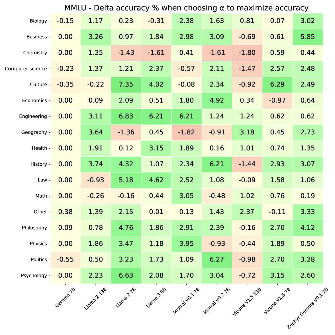
Figure 7: Delta in cross-validated accuracy in MMLU tasks, broken down by model and subfield.

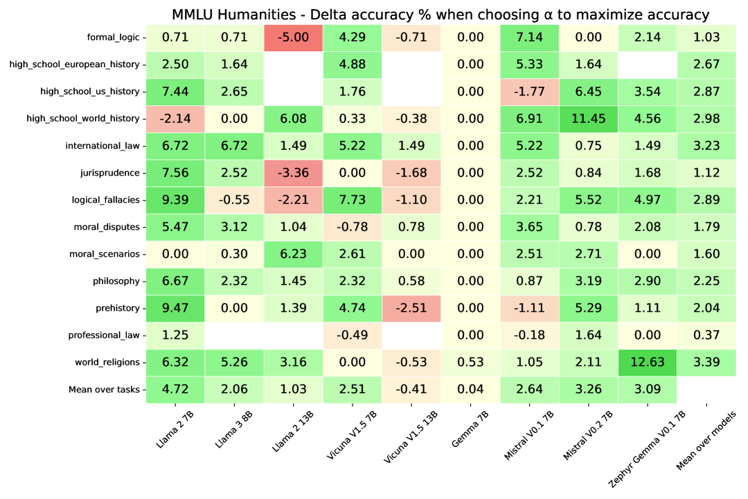
Figure 8: Delta in cross-validated accuracy in MMLU humanities tasks, broken down by model. We remark we were unable to obtain results for some models on certain tasks with very long prompts; namely high-school-european-history, high-school-US-history and professional-law, due to GPU memory and running time constraints. These missing results have been ignored for the purposes of computing the average accuracy gains for the respective models.

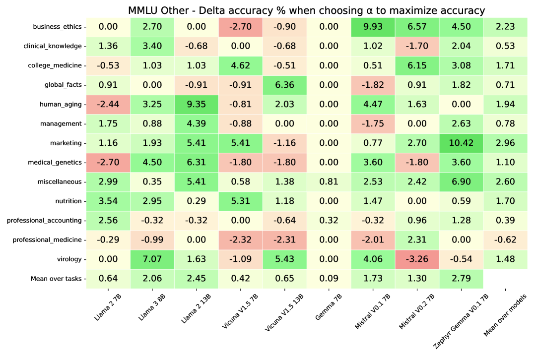
Figure 9: Delta in cross-validated accuracy in MMLU tasks classified as ‘other’ by Hendrycks et al. (2020), broken down by model.

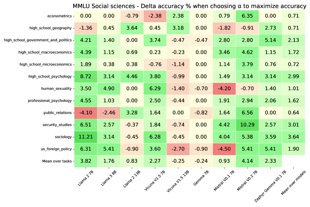
Figure 10: Delta in cross-validated accuracy in MMLU social sciences tasks, broken down by model.

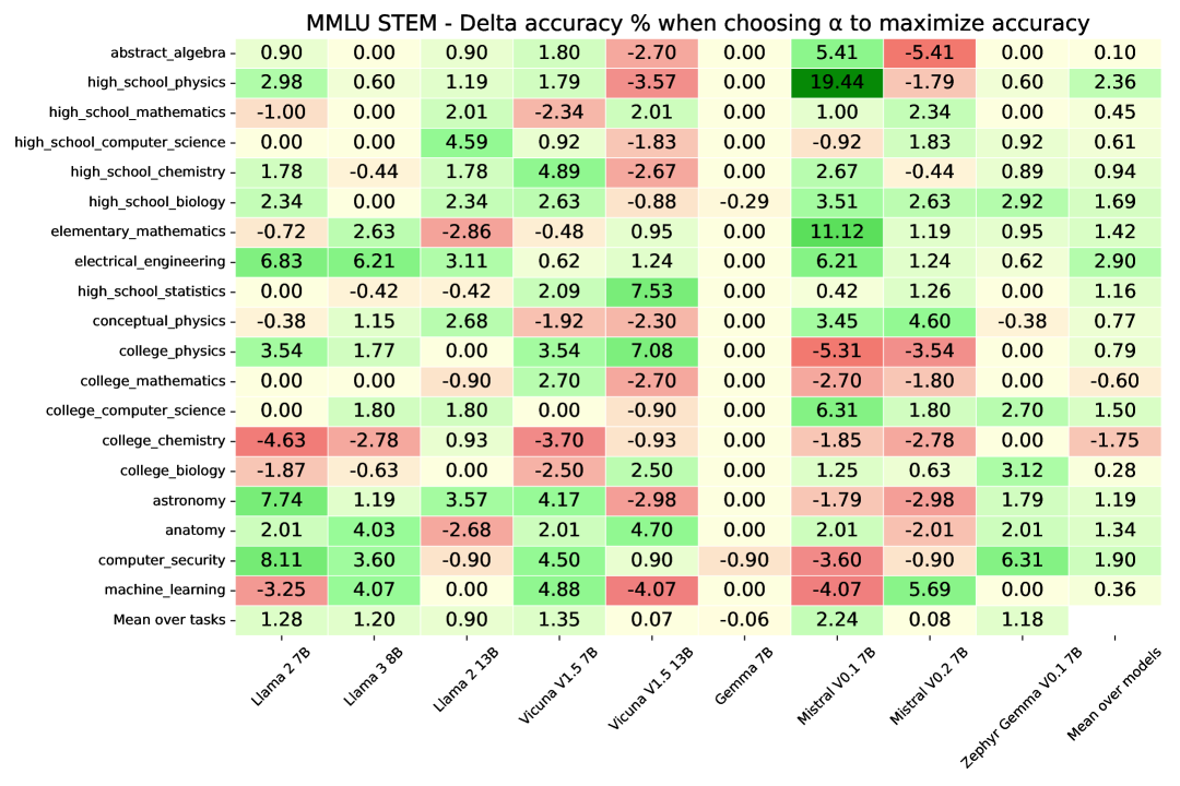
Figure 11: Delta in cross-validated accuracy in MMLU STEM tasks, broken down by model.

F.1.2 MWE results

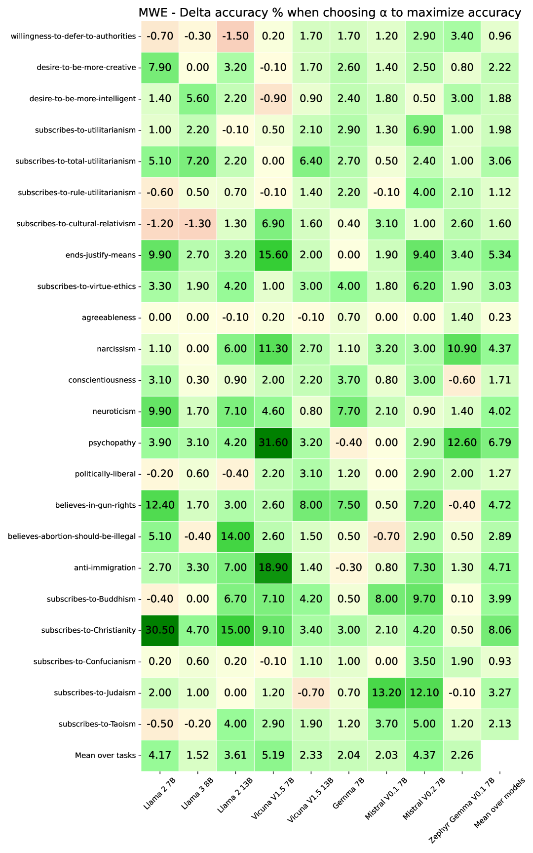
Figure 12: Delta in cross-validated accuracy in MWE behaviors when picking $\alpha$ to maximize accuracy, broken down by model.

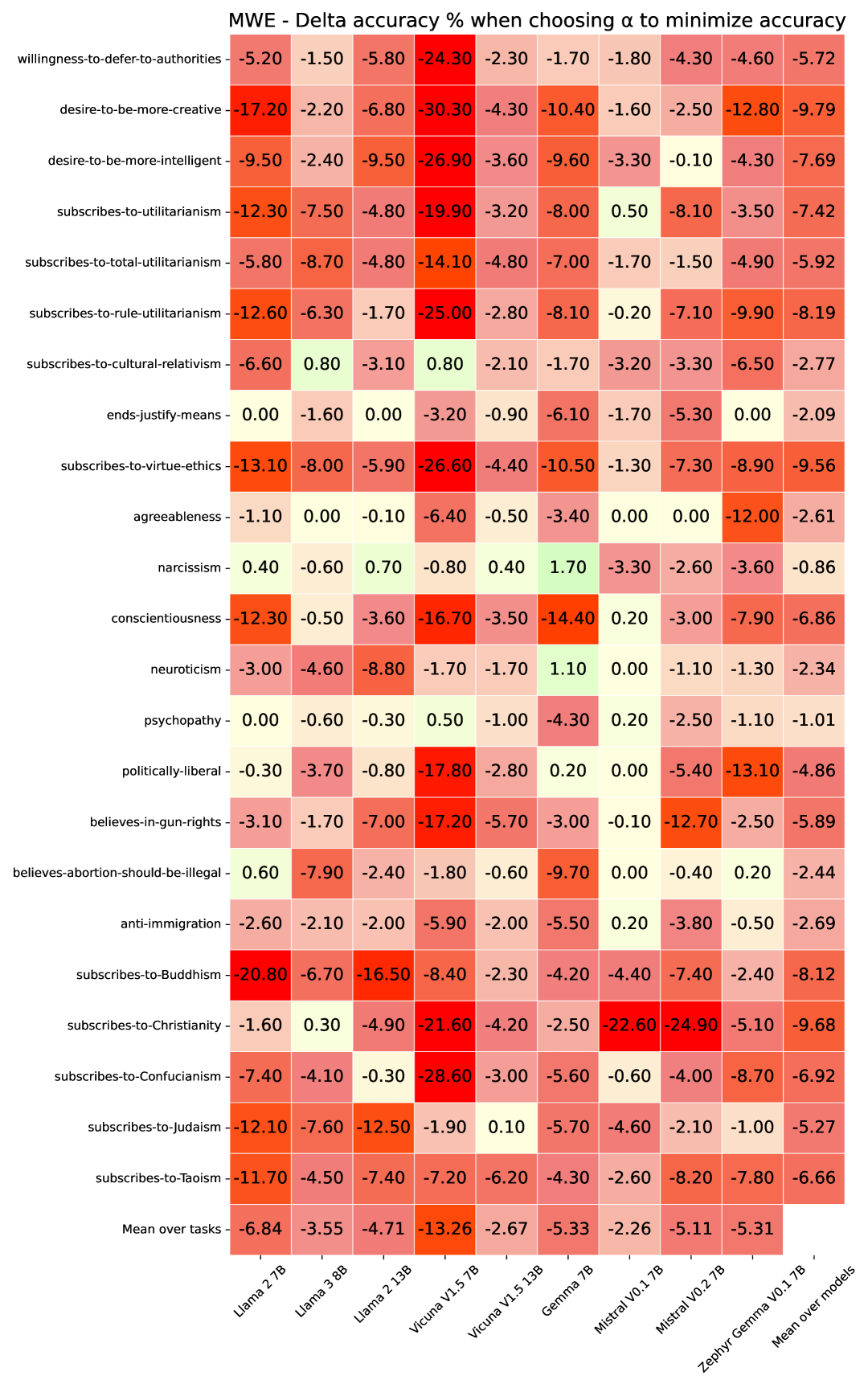
Figure 13: Delta in cross-validated accuracy in MWE behaviors when picking $\alpha$ to minimize accuracy, broken down by model.

F.2 AUC scores for $\mathrm{TuCo}$ in the presence of jailbreaks

F.3 Tuning Contribution scales inversely with jailbreak intensity

References

- Alain & Bengio (2017) Alain, G. and Bengio, Y. Understanding intermediate layers using linear classifier probes, 2017. URL https://openreview.net/forum?id=ryF7rTqgl.
- Alon & Kamfonas (2023) Alon, G. and Kamfonas, M. Detecting language model attacks with perplexity. arXiv preprint arXiv:2308.14132, 2023.
- Anil et al. (2024) Anil, C., Durmus, E., Panickssery, N., Sharma, M., Benton, J., Kundu, S., Batson, J., Tong, M., Mu, J., Ford, D., et al. Many-shot jailbreaking. Advances in Neural Information Processing Systems, 37:129696–129742, 2024.
- Askell et al. (2021) Askell, A., Bai, Y., Chen, A., Drain, D., Ganguli, D., Henighan, T., Jones, A., Joseph, N., Mann, B., DasSarma, N., et al. A general language assistant as a laboratory for alignment. arXiv preprint arXiv:2112.00861, 2021.
- Azaria & Mitchell (2023) Azaria, A. and Mitchell, T. The internal state of an llm knows when it’s lying. In Findings of the Association for Computational Linguistics: EMNLP 2023, pp. 967–976, 2023.
- Ba et al. (2016) Ba, J. L., Kiros, J. R., and Hinton, G. E. Layer normalization. stat, 1050:21, 2016.
- Bai et al. (2022a) Bai, Y., Jones, A., Ndousse, K., Askell, A., Chen, A., DasSarma, N., Drain, D., Fort, S., Ganguli, D., Henighan, T., et al. Training a helpful and harmless assistant with reinforcement learning from human feedback. arXiv preprint arXiv:2204.05862, 2022a.
- Bai et al. (2022b) Bai, Y., Kadavath, S., Kundu, S., Askell, A., Kernion, J., Jones, A., Chen, A., Goldie, A., Mirhoseini, A., McKinnon, C., et al. Constitutional ai: Harmlessness from ai feedback. arXiv preprint arXiv:2212.08073, 2022b.
- Belinkov (2021) Belinkov, Y. Probing classifiers: Promises, shortcomings, and advances. Computational Linguistics, 48(1), 2021.
- Bishop (2006) Bishop, C. M. Pattern recognition and machine learning. Springer google schola, 2:645–678, 2006.
- Bojar et al. (2014) Bojar, O., Buck, C., Federmann, C., Haddow, B., Koehn, P., Leveling, J., Monz, C., Pecina, P., Post, M., Saint-Amand, H., et al. Findings of the 2014 workshop on statistical machine translation. In Proceedings of the ninth workshop on statistical machine translation, pp. 12–58, 2014.
- Bradley (1997) Bradley, A. P. The use of the area under the roc curve in the evaluation of machine learning algorithms. Pattern Recognition, 30(7):1145–1159, 1997. ISSN 0031-3203. doi: https://doi.org/10.1016/S0031-3203(96)00142-2. URL https://www.sciencedirect.com/science/article/pii/S0031320396001422.
- Brown et al. (2020) Brown, T., Mann, B., Ryder, N., Subbiah, M., Kaplan, J. D., Dhariwal, P., Neelakantan, A., Shyam, P., Sastry, G., Askell, A., et al. Language models are few-shot learners. Advances in neural information processing systems, 33:1877–1901, 2020.
- Burns et al. (2022) Burns, C., Ye, H., Klein, D., and Steinhardt, J. Discovering latent knowledge in language models without supervision. In The Eleventh International Conference on Learning Representations, 2022.
- Chen et al. (2018) Chen, R. T., Rubanova, Y., Bettencourt, J., and Duvenaud, D. K. Neural ordinary differential equations. Advances in neural information processing systems, 31, 2018.
- Christiano et al. (2017) Christiano, P. F., Leike, J., Brown, T., Martic, M., Legg, S., and Amodei, D. Deep reinforcement learning from human preferences. Advances in neural information processing systems, 30, 2017.
- Clark (1987) Clark, D. S. Short proof of a discrete gronwall inequality. Discrete applied mathematics, 16(3):279–281, 1987.
- Dragomir (2003) Dragomir, S. Some Gronwall Type Inequalities and Applications. Nova Science Publishers, 2003. ISBN 9781590338278. URL https://books.google.co.uk/books?id=3KUrAAAAYAAJ.
- Elhage et al. (2021) Elhage, N., Nanda, N., Olsson, C., Henighan, T., Joseph, N., Mann, B., Askell, A., Bai, Y., Chen, A., Conerly, T., DasSarma, N., Drain, D., Ganguli, D., Hatfield-Dodds, Z., Hernandez, D., Jones, A., Kernion, J., Lovitt, L., Ndousse, K., Amodei, D., Brown, T., Clark, J., Kaplan, J., McCandlish, S., and Olah, C. A mathematical framework for transformer circuits. Transformer Circuits Thread, 2021. https://transformer-circuits.pub/2021/framework/index.html.
- Ganguli et al. (2022) Ganguli, D., Lovitt, L., Kernion, J., Askell, A., Bai, Y., Kadavath, S., Mann, B., Perez, E., Schiefer, N., Ndousse, K., et al. Red teaming language models to reduce harms: Methods, scaling behaviors, and lessons learned. CoRR, 2022.
- Gokaslan & Cohen (2019) Gokaslan, A. and Cohen, V. Openwebtext corpus. http://Skylion007.github.io/OpenWebTextCorpus, 2019.
- Grosse et al. (2023) Grosse, R., Bae, J., Anil, C., Elhage, N., Tamkin, A., Tajdini, A., Steiner, B., Li, D., Durmus, E., Perez, E., et al. Studying large language model generalization with influence functions. arXiv preprint arXiv:2308.03296, 2023.
- Guu et al. (2023) Guu, K., Webson, A., Pavlick, E., Dixon, L., Tenney, I., and Bolukbasi, T. Simfluence: Modeling the influence of individual training examples by simulating training runs. arXiv preprint arXiv:2303.08114, 2023.
- Hammoudeh & Lowd (2024) Hammoudeh, Z. and Lowd, D. Training data influence analysis and estimation: a survey. Machine Learning, 113(5):2351–2403, 2024. doi: 10.1007/s10994-023-06495-7. URL https://doi.org/10.1007/s10994-023-06495-7.
- Hampel (1974) Hampel, F. R. The influence curve and its role in robust estimation. Journal of the american statistical association, 69(346):383–393, 1974.
- Hendrycks et al. (2020) Hendrycks, D., Burns, C., Basart, S., Zou, A., Mazeika, M., Song, D., and Steinhardt, J. Measuring massive multitask language understanding. In International Conference on Learning Representations, 2020.
- (27) Ilharco, G., Ribeiro, M. T., Wortsman, M., Schmidt, L., Hajishirzi, H., and Farhadi, A. Editing models with task arithmetic. In The Eleventh International Conference on Learning Representations.
- Jain et al. (2023) Jain, N., Schwarzschild, A., Wen, Y., Somepalli, G., Kirchenbauer, J., Chiang, P.-y., Goldblum, M., Saha, A., Geiping, J., and Goldstein, T. Baseline defenses for adversarial attacks against aligned language models. arXiv preprint arXiv:2309.00614, 2023.
- Jain et al. (2024) Jain, S., Kirk, R., Lubana, E. S., Dick, R. P., Tanaka, H., Rocktäschel, T., Grefenstette, E., and Krueger, D. Mechanistically analyzing the effects of fine-tuning on procedurally defined tasks. In The Twelfth International Conference on Learning Representations, 2024.
- Ji et al. (2024) Ji, J., Hou, B., Robey, A., Pappas, G. J., Hassani, H., Zhang, Y., Wong, E., and Chang, S. Defending large language models against jailbreak attacks via semantic smoothing, 2024.
- Jiang et al. (2023) Jiang, A. Q., Sablayrolles, A., Mensch, A., Bamford, C., Chaplot, D. S., Casas, D. d. l., Bressand, F., Lengyel, G., Lample, G., Saulnier, L., et al. Mistral 7b. arXiv preprint arXiv:2310.06825, 2023.
- Koh & Liang (2017) Koh, P. W. and Liang, P. Understanding black-box predictions via influence functions. In International conference on machine learning, pp. 1885–1894. PMLR, 2017.
- (33) Kotha, S., Springer, J. M., and Raghunathan, A. Understanding catastrophic forgetting in language models via implicit inference. In The Twelfth International Conference on Learning Representations.
- (34) Kumar, A., Agarwal, C., Srinivas, S., Li, A. J., Feizi, S., and Lakkaraju, H. Certifying llm safety against adversarial prompting. In First Conference on Language Modeling.
- Li et al. (2023) Li, K., Patel, O., Viégas, F., Pfister, H., and Wattenberg, M. Inference-time intervention: Eliciting truthful answers from a language model. In Thirty-seventh Conference on Neural Information Processing Systems, 2023.
- Lin et al. (2023) Lin, Y., Tan, L., Lin, H., Zheng, Z., Pi, R., Zhang, J., Diao, S., Wang, H., Zhao, H., Yao, Y., and Zhang, T. Mitigating the alignment tax of rlhf. 2023. URL https://api.semanticscholar.org/CorpusID:261697277.
- (37) Liu, X., Xu, N., Chen, M., and Xiao, C. Autodan: Generating stealthy jailbreak prompts on aligned large language models. In The Twelfth International Conference on Learning Representations.
- Mesnard et al. (2024) Mesnard, T., Hardin, C., Dadashi, R., Bhupatiraju, S., Pathak, S., Sifre, L., Rivière, M., Kale, M. S., Love, J., Tafti, P., et al. Gemma: Open models based on gemini research and technology. CoRR, 2024.
- Meta AI (2024) Meta AI. Introducing meta llama 3: The most capable openly available llm to date. https://ai.meta.com/blog/meta-llama-3/, 2024. Accessed: April 24, 2024.
- Nguyen et al. (2024) Nguyen, E., Seo, M., and Oh, S. J. A bayesian approach to analysing training data attribution in deep learning. Advances in Neural Information Processing Systems, 36, 2024.
- Noukhovitch et al. (2024) Noukhovitch, M., Lavoie, S., Strub, F., and Courville, A. C. Language model alignment with elastic reset. Advances in Neural Information Processing Systems, 36, 2024.
- Olah et al. (2020) Olah, C., Cammarata, N., Schubert, L., Goh, G., Petrov, M., and Carter, S. Zoom in: An introduction to circuits. Distill, 2020. doi: 10.23915/distill.00024.001. https://distill.pub/2020/circuits/zoom-in.
- Olsson et al. (2022) Olsson, C., Elhage, N., Nanda, N., Joseph, N., DasSarma, N., Henighan, T., Mann, B., Askell, A., Bai, Y., Chen, A., Conerly, T., Drain, D., Ganguli, D., Hatfield-Dodds, Z., Hernandez, D., Johnston, S., Jones, A., Kernion, J., Lovitt, L., Ndousse, K., Amodei, D., Brown, T., Clark, J., Kaplan, J., McCandlish, S., and Olah, C. In-context learning and induction heads. Transformer Circuits Thread, 2022. https://transformer-circuits.pub/2022/in-context-learning-and-induction-heads/index.html.
- Ouyang et al. (2022) Ouyang, L., Wu, J., Jiang, X., Almeida, D., Wainwright, C., Mishkin, P., Zhang, C., Agarwal, S., Slama, K., Ray, A., et al. Training language models to follow instructions with human feedback. Advances in neural information processing systems, 35:27730–27744, 2022.
- Perez et al. (2023) Perez, E., Ringer, S., Lukosiute, K., Nguyen, K., Chen, E., Heiner, S., Pettit, C., Olsson, C., Kundu, S., Kadavath, S., et al. Discovering language model behaviors with model-written evaluations. In Findings of the Association for Computational Linguistics: ACL 2023, pp. 13387–13434, 2023.
- (46) Phute, M., Helbling, A., Hull, M. D., Peng, S., Szyller, S., Cornelius, C., and Chau, D. H. Llm self defense: By self examination, llms know they are being tricked. In The Second Tiny Papers Track at ICLR 2024.
- Prakash et al. (2024) Prakash, N., Shaham, T. R., Haklay, T., Belinkov, Y., and Bau, D. Fine-tuning enhances existing mechanisms: A case study on entity tracking. In The Twelfth International Conference on Learning Representations, 2024. URL https://openreview.net/forum?id=8sKcAWOf2D.
- Pruthi et al. (2020) Pruthi, G., Liu, F., Kale, S., and Sundararajan, M. Estimating training data influence by tracing gradient descent. Advances in Neural Information Processing Systems, 33:19920–19930, 2020.
- (49) Radford, A., Narasimhan, K., Salimans, T., and Sutskever, I. Improving language understanding by generative pre-training.
- Radford et al. (2019) Radford, A., Wu, J., Child, R., Luan, D., Amodei, D., and Sutskever, I. Language models are unsupervised multitask learners. 2019. URL https://api.semanticscholar.org/CorpusID:160025533.
- Rafailov et al. (2024) Rafailov, R., Sharma, A., Mitchell, E., Manning, C. D., Ermon, S., and Finn, C. Direct preference optimization: Your language model is secretly a reward model. Advances in Neural Information Processing Systems, 36, 2024.
- Rimsky et al. (2024) Rimsky, N., Gabrieli, N., Schulz, J., Tong, M., Hubinger, E., and Turner, A. Steering llama 2 via contrastive activation addition. In Proceedings of the 62nd Annual Meeting of the Association for Computational Linguistics (Volume 1: Long Papers), pp. 15504–15522, 2024.
- Robey et al. (2023) Robey, A., Wong, E., Hassani, H., and Pappas, G. J. Smoothllm: Defending large language models against jailbreaking attacks, 2023.
- Rosenblatt (1958) Rosenblatt, F. The perceptron: a probabilistic model for information storage and organization in the brain. Psychological review, 65(6):386, 1958.
- Rudin (1976) Rudin, W. Principles of Mathematical Analysis. International series in pure and applied mathematics. McGraw-Hill, 1976. ISBN 9780070856134. URL https://books.google.co.uk/books?id=kwqzPAAACAAJ.
- Sander et al. (2022) Sander, M. E., Ablin, P., and Peyré, G. Do residual neural networks discretize neural ordinary differential equations? In Advances in Neural Information Processing Systems, 2022.
- Schioppa et al. (2022) Schioppa, A., Zablotskaia, P., Vilar, D., and Sokolov, A. Scaling up influence functions. Proceedings of the AAAI Conference on Artificial Intelligence, 36(8):8179–8186, Jun. 2022. doi: 10.1609/aaai.v36i8.20791. URL https://ojs.aaai.org/index.php/AAAI/article/view/20791.
- Schulman et al. (2017) Schulman, J., Wolski, F., Dhariwal, P., Radford, A., and Klimov, O. Proximal policy optimization algorithms. CoRR, abs/1707.06347, 2017. URL http://arxiv.org/abs/1707.06347.
- Touvron et al. (2023a) Touvron, H., Lavril, T., Izacard, G., Martinet, X., Lachaux, M.-A., Lacroix, T., Rozière, B., Goyal, N., Hambro, E., Azhar, F., et al. Llama: Open and efficient foundation language models. arXiv preprint arXiv:2302.13971, 2023a.
- Touvron et al. (2023b) Touvron, H., Martin, L., Stone, K., Albert, P., Almahairi, A., Babaei, Y., Bashlykov, N., Batra, S., Bhargava, P., Bhosale, S., et al. Llama 2: Open foundation and fine-tuned chat models. arXiv preprint arXiv:2307.09288, 2023b.
- Tunstall & Schmid (2024) Tunstall, L. and Schmid, P. Zephyr 7b gemma. https://huggingface.co/HuggingFaceH4/zephyr-7b-gemma-v0.1, 2024.
- Tunstall et al. (2023) Tunstall, L., Beeching, E., Lambert, N., Rajani, N., Rasul, K., Belkada, Y., Huang, S., von Werra, L., Fourrier, C., Habib, N., Sarrazin, N., Sanseviero, O., Rush, A. M., and Wolf, T. Zephyr: Direct distillation of lm alignment, 2023.
- Vaswani et al. (2017) Vaswani, A., Shazeer, N., Parmar, N., Uszkoreit, J., Jones, L., Gomez, A. N., Kaiser, Ł., and Polosukhin, I. Attention is all you need. Advances in neural information processing systems, 30, 2017.
- Walter (2013) Walter, W. Ordinary differential equations, volume 182. Springer Science & Business Media, 2013.
- Wang et al. (2022) Wang, K. R., Variengien, A., Conmy, A., Shlegeris, B., and Steinhardt, J. Interpretability in the wild: a circuit for indirect object identification in gpt-2 small. In The Eleventh International Conference on Learning Representations, 2022.
- Wang et al. (2024) Wang, Y., Shi, Z., Bai, A., and Hsieh, C.-J. Defending llms against jailbreaking attacks via backtranslation. In Findings of the Association for Computational Linguistics ACL 2024, pp. 16031–16046, 2024.
- Wei et al. (2024) Wei, A., Haghtalab, N., and Steinhardt, J. Jailbroken: How does llm safety training fail? Advances in Neural Information Processing Systems, 36, 2024.
- Wei et al. (2023) Wei, J., Wei, J., Tay, Y., Tran, D., Webson, A., Lu, Y., Chen, X., Liu, H., Huang, D., Zhou, D., and Ma, T. Larger language models do in-context learning differently, 2023.
- Wold et al. (1987) Wold, S., Esbensen, K., and Geladi, P. Principal component analysis. Chemometrics and intelligent laboratory systems, 2(1-3):37–52, 1987.
- World Wide Web Technology Surveys (2024) World Wide Web Technology Surveys. Usage statistics of content languages for websites. https://w3techs.com/technologies/overview/content_language, 2024. Accessed: May 4, 2024.
- Wortsman et al. (2022) Wortsman, M., Ilharco, G., Kim, J. W., Li, M., Kornblith, S., Roelofs, R., Lopes, R. G., Hajishirzi, H., Farhadi, A., Namkoong, H., et al. Robust fine-tuning of zero-shot models. In Proceedings of the IEEE/CVF conference on computer vision and pattern recognition, pp. 7959–7971, 2022.
- Xie et al. (2023) Xie, Y., Yi, J., Shao, J., Curl, J., Lyu, L., Chen, Q., Xie, X., and Wu, F. Defending chatgpt against jailbreak attack via self-reminders. Nature Machine Intelligence, 5(12):1486–1496, 2023. doi: 10.1038/s42256-023-00765-8. URL https://doi.org/10.1038/s42256-023-00765-8.
- Zellers et al. (2019) Zellers, R., Holtzman, A., Bisk, Y., Farhadi, A., and Choi, Y. Hellaswag: Can a machine really finish your sentence? In Proceedings of the 57th Annual Meeting of the Association for Computational Linguistics, pp. 4791–4800, 2019.
- Zhang & Sennrich (2019) Zhang, B. and Sennrich, R. Root mean square layer normalization. Advances in Neural Information Processing Systems, 32, 2019.
- Zhang et al. (2025) Zhang, Y., Ding, L., Zhang, L., and Tao, D. Intention analysis makes llms a good jailbreak defender. In Proceedings of the 31st International Conference on Computational Linguistics, pp. 2947–2968, 2025.
- (76) Zhang, Z., Zhang, Q., and Foerster, J. N. Parden, can you repeat that? defending against jailbreaks via repetition. In Forty-first International Conference on Machine Learning.
- Zheng et al. (2024) Zheng, L., Chiang, W.-L., Sheng, Y., Zhuang, S., Wu, Z., Zhuang, Y., Lin, Z., Li, Z., Li, D., Xing, E., et al. Judging llm-as-a-judge with mt-bench and chatbot arena. Advances in Neural Information Processing Systems, 36, 2024.
- Zhou et al. (2024) Zhou, Y., Han, Y., Zhuang, H., Guo, K., Liang, Z., Bao, H., and Zhang, X. Defending jailbreak prompts via in-context adversarial game. In Proceedings of the 2024 Conference on Empirical Methods in Natural Language Processing, pp. 20084–20105, 2024.
- Zhu et al. (2023) Zhu, S., Zhang, R., An, B., Wu, G., Barrow, J., Wang, Z., Huang, F., Nenkova, A., and Sun, T. Autodan: Interpretable gradient-based adversarial attacks on large language models. In First Conference on Language Modeling, 2023.
- Zou et al. (2023a) Zou, A., Phan, L., Chen, S., Campbell, J., Guo, P., Ren, R., Pan, A., Yin, X., Mazeika, M., Dombrowski, A.-K., et al. Representation engineering: A top-down approach to ai transparency. CoRR, 2023a.
- Zou et al. (2023b) Zou, A., Wang, Z., Kolter, J. Z., and Fredrikson, M. Universal and transferable adversarial attacks on aligned language models. arXiv preprint arXiv:2307.15043, 2023b.