Computing Multi-Lumps in Nonlinearity-Managed Spatial-Symmetric Dispersive Framework

Abstract.

We investigate the dynamics of multi-lump waves in a generalized spatial symmetric higher-dimensional dispersive water wave model using an analytical approach. This involves the construction of explicit solutions using Hirota’s bilinear method and generalized polynomial expansions. The dynamical study shows that the multi-lump waves are non-interacting and reveal different geometrical patterns.

1. Introduction

The manifestation of localized coherent structures in physical systems is one of the most intriguing phenomena in nature. The classical stable coherent structure, the solitons, appears in dispersive models with a delicate balance between nonlinearity and dispersion. A variety of one- and higher-dimensional models are proposed for the exploration of exotic wave patterns such as solitary waves, breathers, cnoidal waves, compactons, rogue waves, and lumps, where each of them is characterized by distinct dynamical features and localization properties [Yan10]. Recently, spatially symmetric nonlinear models have attracted considerable interest, and a few works have been reported in the literature for the investigation of localized wave structures, particularly solitons and lump wave solutions. To be specific, a (2+1)-dimensional spatially symmetric Hirota-Satsuma-Ito model has been analyzed for lump waves in [MBA21]. Similarly, a (2+1)-dimensional dispersive water wave model with spatial symmetry is examined in [Ma23]. The lump waves in the spatially symmetric KP model are reported in [MBM23], while a generalized spatially symmetric KP-type model is proposed in [Ma24] with lump waves, breather solitons [ZMM⁺24] and interaction solutions [Kan25]. These works deal with (2+1)-dimensional models and first-order lump and interactions and breather wave profiles.

Motivated by these developments and several open questions because of the new problem, we propose the following generalized (3+1)-dimensional spatial symmetric dispersive water wave model and aim to investigate multi-lump wave by constructing explicit solutions and analysis thereof:

(1.1) $$P(u,v,w,r) =\alpha_{1}\left(u_{xt}+6u_{x}v_{x}+6u_{xx}v\right)+\alpha_{2}u_{xxxx}+\alpha_{3}u_{xx}$$

$$\quad+\beta_{1}\left(u_{yt}+6u_{y}w_{y}+6u_{yy}w\right)+\beta_{2}u_{yyyy}+\beta_{3}u_{yy}$$

$$\quad+\gamma_{1}\left(u_{zt}+6u_{z}r_{z}+6u_{zz}r\right)+\gamma_{2}u_{zzzz}+\gamma_{3}u_{zz}=0,$$

where $v_{y}=u_{x}$, $w_{x}=u_{y}$ and $r_{x}=u_{z}$, with $u$ being a function of $x$, $y$, $z$ and $t$. The manuscript is organized as follows. In the next section, we construct first-order lump wave solutions. Section 3 is devoted to the analysis of second- and third-order lump waves. Finally, concluding remarks are presented in the last section.

2. The method and First-order lump-wave solution

In this section, we study the evolutionary dynamics of the first lump wave of the new generalized (3+1)-dimensional spatial symmetric dispersive-nonlinear wave (GSSDNW) model (1.1). To achieve this, we make use of the dimensional reduction and Hirota’s bilinear methods. First, we transform the GSSDNW equation (1.1) to a $(1+1)$-dimensional nonlinear equation through the dimensional reduction approach using $\tau=(mx+nt)$, $\xi=(\mu y+\lambda z)$, thereby applying the following set of logarithmic transformations:

$$u(\xi,\tau)=2(\ln f)_{\tau\xi},\quad v(\xi,\tau)=2(\ln f)_{\tau\tau},\quad w(\xi,\tau)=2(\ln f)_{\xi\xi},\quad r(\xi,\tau)=2(\ln f)_{\xi\xi}.$$

From further simplification, we arrive at the Hirota bilinear equation described as

(2.1) $$\left(\chi_{1}D_{\tau}^{4}+\chi_{2}D_{\xi}^{4}+\chi_{3}D_{\tau}^{2}+\chi_{4}D_{\xi}^{2}+\chi_{5}D_{\tau}D_{\xi}\right)f\cdot f=0,$$

where

$$\chi_{1}=(2m^{4}\alpha_{2}\gamma_{2}),\quad\chi_{2}=(\gamma_{1}^{2}+2\beta_{1}\gamma_{2}\mu^{2}-\gamma_{0}\gamma_{1}),\quad\chi_{3}=2\gamma_{2}m^{2}(\alpha_{3}+mn\alpha_{2}),$$

$$\chi_{4}=(\gamma_{1}\gamma_{3}+2\beta_{3}\gamma_{2}\mu^{2}-\gamma_{0}\gamma_{3}),\quad\chi_{5}=2\gamma_{2}n\left(\beta_{1}\mu+\gamma_{1}\lambda\right).$$

The above bilinearizing process possesses certain restrictions among the parameters as below.

$$\alpha_{2}=(\alpha_{1}/{m^{2}})\,;\quad\lambda=\sqrt{\left({\gamma_{1}-\gamma_{0}}\right)/{2\gamma_{2}}};\quad\mbox{where}\quad\gamma_{0}=\sqrt{(\gamma_{1}^{2}+4\beta_{1}\gamma_{2}\mu^{2}-4\beta_{2}\gamma_{2}\mu^{4})},$$

which can serve as the integrability constraints for the reduced $(1+1)$-dimensional nonlinear model. In the bilinear equation, $D$ is the Hirota bilinear operator defined as follows [Hir04].

(2.2) $$D_{\tau}^{a}D_{\xi}^{b}(\Lambda\cdot\Theta)=\left(\frac{\partial}{\partial\tau}-\frac{\partial}{\partial\tau^{\prime}}\right)^{a}\left(\frac{\partial}{\partial\xi}-\frac{\partial}{\partial\xi^{\prime}}\right)^{b}\Lambda(\xi,\tau)\,\Theta(\tau^{\prime},\xi^{\prime})\Big{|}_{\tau^{\prime}=\tau,\,\xi^{\prime}=\xi}.$$

To construct the first-order lump-wave solution, we choose the following test function:

(2.3) $$f(\xi,\tau)=a_{0,0}+a_{0,2}\xi^{2}+a_{2,0}\tau^{2}+a_{1,1}\xi\tau,$$

where $a_{0,0}$, $a_{0,2}$, $a_{2,0}$, and $a_{1,1}$ are constants to be determined. On substituting the above ansatz into the bilinear equation (2.1) and solving it recursively, we get the following explicit form for the parameters:

$$a_{0,0}=-\frac{12\left(\chi_{2}\chi_{3}^{2}+\chi_{1}\chi_{4}^{2}\right)}{\chi_{3}\left(4\chi_{3}\chi_{4}-\chi_{5}^{2}\right)},\quad a_{2,0}=\frac{\chi_{4}}{\chi_{3}},\quad a_{1,1}=-\frac{\chi_{5}}{\chi_{3}},\quad a_{0,2}=1.$$

Substituting the above parameters into equation (2.3), applying the logarithmic variable transformation and going back to the original model using the dimensional reduction, we obtain the required first-order lump wave solution. The obtained solution contains various arbitrary parameters, using which one can manipulate the dynamical characteristics of the resulting lump waves. The evolution of such a first-order lump wave is depicted in Fig. 1.

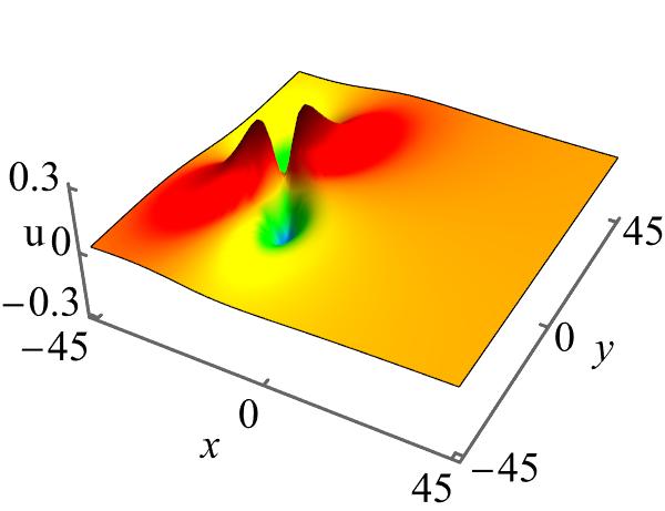
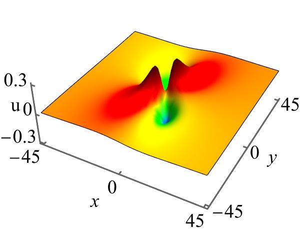
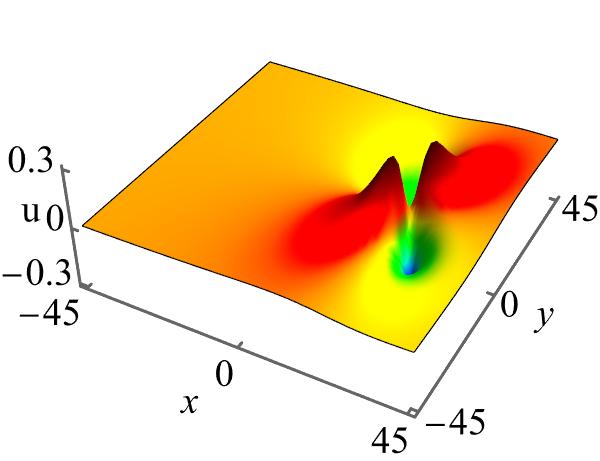
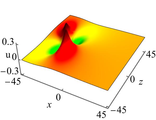
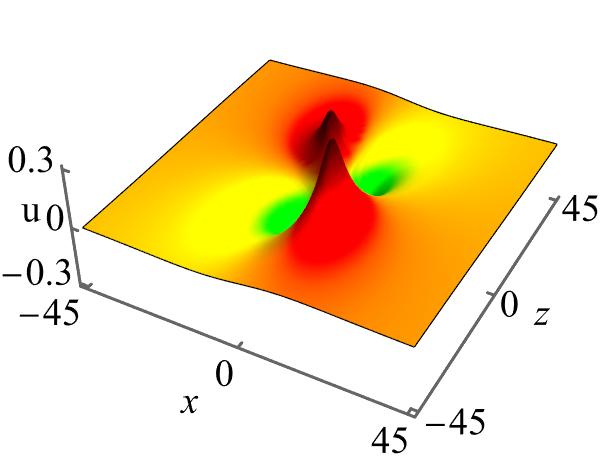
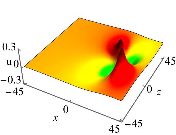
Figure 1. Evolution of first-order lump structure in the $x$–$y$ and $x$–$z$ planes at $z=0.1$ and $y=0.1$, respectively, at different times $t=-15~((a)~\&~(d))$, $t=0~((b)~\&~(e))$, and $t=15~((c)~\&~(f))$. The remaining parameters are taken as $\gamma_{1}=3$, $\gamma_{2}=3$, $m=0.2$, $n=-0.3$, $\alpha_{3}=\alpha_{2}=-0.4$, $\mu=-0.5$, $\beta_{3}=2$, $\gamma_{3}=-3.1$, $\beta_{1}=3$, and $\beta_{2}=21$.

It is evident from Fig. 1 that the obtained first-order lump wave possesses a paired peak, and they do not interact during evolution. Note that the nature of the present lump waves differs along the three spatial dimensions. Basically, the orientation of the lump waves and their peaks change along the way, as demonstrated in Fig. 1 for an example. By changing other arbitrary parameters, the properties of the lump waves, such as amplitude, thickness/width, spacing between the peaks, along with the orientation, can be controlled effectively. Considering the length of the manuscript, we have not provided further details and graphical explanations.

3. Higher-order Lump Waves

To derive the higher-order lump wave solutions of the considered GSSDNW model (1.1), we incorporate technical input from the previous reports given in [GHLM21, Pen21]. By imposing the constraint conditions, we wish to eliminate the contribution of the mixed Hirota derivative $D_{\xi}D_{\tau}$ and the fourth-order Hirota derivative $D_{\xi}^{4}$, thereby simplifying the underlying model. Taking into account the constraint condition $\chi_{2}=\chi_{5}=0$, the following restrictions have to be imposed:

$$\beta_{1}=2\beta_{2}\mu^{2},\quad\gamma_{1}=-\beta_{1},\quad\gamma_{2}=-\beta_{2}.$$

To construct higher-order lump wave solutions, we take a generalized polynomial function for $f(\xi,\tau)$ by following Refs. [CD17, Zha18, GHLM21] as given below.

(3.1) $$f(\xi,\tau)=F_{n+1}(\xi,\tau)+2\phi\,\xi\,P_{n}(\xi,\tau)+2\psi\,\tau\,Q_{n}(\xi,\tau)+(\phi^{2}+\psi^{2})\,F_{n-1}(\xi,\tau),$$

where

$$F_{n}(\xi,\tau)=\sum_{k=0}^{n(n+1)/2}\sum_{i=0}^{k}a_{n(n+1)-2k,\,2i}\,\xi^{2i}\,\tau^{n(n+1)-2k},$$

$$P_{n}(\xi,\tau)=\sum_{k=0}^{n(n+1)/2}\sum_{i=0}^{k}b_{n(n+1)-2k,\,2i}\,\,\tau^{2i}\,\xi^{n(n+1)-2k},$$

$$Q_{n}(\xi,\tau)=\sum_{k=0}^{n(n+1)/2}\sum_{i=0}^{k}c_{n(n+1)-2k,\,2i}\,\xi^{2i}\,\tau^{n(n+1)-2k}.$$

The application of the above polynomial in the bilinear form and solving the resulting equation, one can arrive at the solution in (1+1)-dimensional version, from which the required solution for the (3+1)D GSSDNW equation can be constructed by using the dimensional-expansion.

As an example, to construct the second-order lump solution, we choose $a_{(n+1)(n+2),\,0}=1$, $F_{0}=1$, and for $n=1$, which terminates the polynomial expansion for $f$ as below.

$$f(\xi,\tau)=F_{2}(\xi,\tau)+2\phi\,\xi\,P_{1}(\xi,\tau)+2\psi\,\tau\,Q_{1}(\xi,\tau)+(\phi^{2}+\psi^{2}).$$

The substitution of $F_{2}(\xi,\tau)$, $P_{1}(\xi,\tau)$, and $Q_{1}(\xi,\tau)$, gives the following detailed form for the test function $f(\xi,\tau)$ corresponding to the second-order lump wave:

$$f(\xi,\tau)= (a_{0,0}+a_{0,2}\xi^{2}+a_{0,4}\xi^{4}+a_{0,6}\xi^{6})+(a_{2,0}+a_{2,2}\xi^{2}+a_{2,4}\xi^{4})\tau^{2}+(a_{4,0}+a_{4,2}\xi^{2})\tau^{4}+\tau^{6}$$

$$+2\phi\xi(b_{0,0}+b_{0,2}\xi^{2}+b_{2,0}\tau^{2})+2\psi\tau(c_{0,0}+c_{0,2}\xi^{2}+c_{2,0}\tau^{2})+(\phi^{2}+\psi^{2})\,.$$

Using the above test function (3) for second-order lump waves in the bilinear equation (2.1), and collecting all terms that involve powers of $\left(\tau^{i}\xi^{j}\right)$, where $\left(i,j=0,1,2,\dots\right)$, we obtain a system of nonlinear algebraic equations. Upon solving this system, we derive the following lump wave parameters corresponding to the second-order lump wave:

$$a_{0,0} =\frac{-16875\,\chi_{1}^{3}+\chi_{3}^{2}\left(\phi^{2}\,(-9\,\chi_{3}+b_{2,0}^{2}\,\chi_{4})+9\,(c_{2,0}^{2}-1)\,\chi_{3}\,\psi^{2}\right)}{9\,\chi_{3}^{3}}\,;\quad a_{0,2}=\frac{475\,\chi_{1}^{2}}{\chi_{3}\,\chi_{4}}\,;$$

$$a_{0,4} =-\frac{17\,\chi_{1}\,\chi_{3}}{\chi_{4}^{2}}\,;\quad a_{0,6}=\left(\frac{\chi_{3}}{\chi_{4}}\right)^{3}\,;\quad a_{2,0}=-125\left(\frac{\,\chi_{1}}{\chi_{3}}\right)^{2}\,;\quad a_{2,2}=-\frac{90\,\chi_{1}}{\chi_{4}}\,;\quad a_{2,4}=3\left(\frac{\,\chi_{3}}{\chi_{4}}\right)^{2}\,;$$

$$a_{4,0} =-\frac{25\,\chi_{1}}{\chi_{3}}\,;\quad a_{4,2}=\frac{3\,\chi_{3}}{\chi_{4}}\,;\quad b_{0,0}=-\frac{5\,b_{2,0}\,\chi_{1}}{3\,\chi_{3}}\,;\quad b_{0,2}=-\frac{b_{2,0}\,\chi_{3}}{3\,\chi_{4}}\,;$$

$$c_{0,0} =\frac{c_{2,0}\,\chi_{1}}{\chi_{3}}\,;\quad c_{0,2}=-\frac{3\,c_{2,0}\,\chi_{3}}{\chi_{4}}\,.$$

The above explicit form of parameters and the final expression $f(\xi,\tau)$ gives the required second-order lump-wave solution of the GSSDNW equation (1.1) from the bilinear transformations and mapping to the original (3+1)-dimensions. This second-order solution contains four arbitrary parameters, namely, $b_{2,0},c_{2,0},\phi$, and $\psi$ apart from the arbitrary model parameters, and using them all, one can modify the nature and evolution of the lump-wave dynamics effectively. For an easy understanding, one such evolution of the second-order lump waves is demonstrated in Fig. 2. It is clear that the second-order lumps exhibit three sets of paired peaks and do not interact during the time evolution. Such a structure resembles the identities of three independent first-order lump-waves, and they combine to form a triangular geometry. As mentioned earlier, the characteristics of the triangular lump waves, like inter- and intra-peak distance, peak amplitude, width of peaks, angle or orientation of the peaks in addition to the orientation of the triangular structure itself, can be tuned by properly adjusting the available arbitrary parameters.

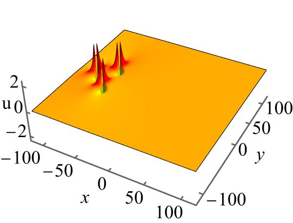
(a) $t=-5$

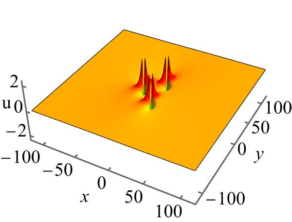
(b) $t=0$

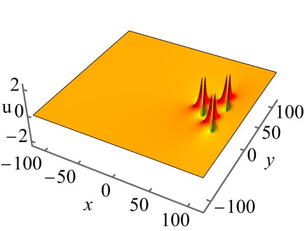
(c) $t=5$

Figure 2. The evolution of second-order lump-wave possessing triangular structure in the $x$–$y$ planes for $z=0.5$ at (a) $t=-5$, (b) $t=0$, and (c) $t=5$, with other parameters taken as $\gamma_{1}=-1$, $\gamma_{2}=-2$, $\mu=0.5$, $\beta_{1}=1$, $\beta_{2}=2$, $m=-0.2$, $n=3$, $\alpha_{3}=-1$, $\alpha_{2}=2$, $\beta_{3}=-3$, $\gamma_{3}=-3.2$, $\phi=2$, $\psi=3$, $b_{2,0}=0.2$, and $c_{2,0}=-10$.

To proceed further for the construction of a third-order lump-wave solution, we terminate the polynomial expansion for $n=2$ and obtain the following form for the function $f(\xi,\tau)$, which will serve as the test function for the third-order lump solution:

$$f(\xi,\tau)=F_{3}(\xi,\tau)+2\phi\,\xi\,P_{2}(\xi,\tau)+2\psi\,\tau\,Q_{2}(\xi,\tau)+(\phi^{2}+\psi^{2})F_{1}(\xi,\tau).$$

where $F_{1}$ is given in $(\ref{eq4})$. By substituting the above $f(\xi,\tau)$ into the bilinear equation and solving the resulting set of algebraic equations recursively, as performed in the previous cases, one can arrive at the explicit form of the parameters as follows.

$$a_{0,0} =\frac{\chi_{1}(878826025\chi_{1}^{5}\chi_{3}^{2}+27\phi^{2}\chi_{3}^{6}\chi_{4}-27\phi^{2}\chi_{4}^{7}-27\chi_{3}^{7}\psi^{2}+27\chi_{3}^{6}\chi_{4}\psi^{2})}{9\chi_{3}^{8}},$$

$$a_{0,2} =\frac{-300896750\chi_{1}^{5}\chi_{3}^{2}-3\phi^{2}\chi_{3}^{6}\chi_{4}+3\phi^{2}\chi_{4}^{7}+3\chi_{3}^{7}\psi^{2}-3\chi_{3}^{6}\chi_{4}\psi^{2}}{3\chi_{3}^{6}\chi_{4}},$$

$$a_{0,4} =\frac{16391725\chi_{1}^{4}}{3\chi_{3}^{2}\chi_{4}^{2}},\quad a_{0,6}=\frac{-798980\chi_{1}^{3}}{3\chi_{4}^{3}},\quad a_{0,8}=\frac{4335\chi_{1}^{2}\chi_{3}^{2}}{\chi_{4}^{4}},\quad a_{0,10}=\frac{-58\chi_{1}\chi_{3}^{4}}{\chi_{4}^{5}},$$

$$a_{0,12} =\frac{\chi_{3}^{6}}{\chi_{4}^{6}},\quad a_{2,0}=\frac{-159786550\chi_{1}^{5}\chi_{3}^{2}-3\phi^{2}\chi_{3}^{6}\chi_{4}+3\phi^{2}\chi_{4}^{7}+3\chi_{3}^{7}\psi^{2}-3\chi_{3}^{6}\chi_{4}\psi^{2}}{{3\chi_{3}^{7}}},$$

$$a_{2,2} =\frac{565950\chi_{1}^{4}}{\chi_{3}^{3}\chi_{4}},\quad a_{2,4}=\frac{14700\chi_{1}^{3}}{\chi_{3}\chi_{4}^{2}},\quad a_{2,6}=\frac{35420\chi_{1}^{2}\chi_{3}}{\chi_{4}^{3}},\quad a_{2,8}=\frac{-570\chi_{1}\chi_{3}^{3}}{\chi_{4}^{4}},\quad a_{2,10}=\frac{6\chi_{3}^{5}}{\chi_{4}^{5}},$$

$$a_{4,0} =\frac{-5187875\chi_{1}^{4}}{3\chi_{3}^{4}},\quad a_{4,2}=\frac{220500\chi_{1}^{3}}{\chi_{3}^{2}\chi_{4}},\quad a_{4,4}=\frac{37450\chi_{1}^{2}}{\chi_{4}^{2}},\quad a_{4,6}=\frac{-1460\chi_{1}\chi_{3}^{2}}{\chi_{4}^{3}},\quad a_{4,8}=\frac{15\chi_{3}^{4}}{\chi_{4}^{4}},$$

$$a_{6,0} =\frac{-75460\chi_{1}^{3}}{3\chi_{3}^{3}},\quad a_{6,2}=\frac{18620\chi_{1}^{2}}{\chi_{3}\chi_{4}},\quad a_{6,4}=\frac{-1540\chi_{1}\chi_{3}}{\chi_{4}^{2}},\quad a_{6,6}=\frac{20{\chi_{3}^{3}}}{\chi_{4}^{3}},\quad a_{8,0}=\frac{735\chi_{1}^{2}}{\chi_{3}^{2}},$$

$$a_{8,2} =\frac{-690\chi_{1}}{\chi_{4}},\quad a_{8,4}=\frac{15\chi_{3}^{2}}{\chi_{4}^{2}},\quad a_{10,0}=\frac{-98\chi_{1}}{\chi_{3}},\quad a_{10,2}=\frac{6\chi_{3}}{\chi_{4}},\quad b_{0,0}=\frac{-18865\chi_{1}^{3}\chi_{4}^{3}}{3\chi_{3}^{6}},$$

$$b_{0,2} =\frac{-665\chi_{1}^{2}\chi_{4}^{3}}{\chi_{3}^{5}},\quad b_{0,4}=\frac{-105\chi_{1}\chi_{4}^{3}}{\chi_{3}^{4}},\quad b_{0,6}=\frac{5\chi_{4}^{3}}{\chi_{3}^{3}},\quad b_{2,0}=\frac{-245\chi_{1}^{2}\chi_{4}^{2}}{\chi_{3}^{4}},\quad b_{2,2}=\frac{190\chi_{1}\chi_{4}^{2}}{\chi_{3}^{3}},$$

$$b_{2,4} =\frac{-5\chi_{4}^{2}}{\chi_{3}^{2}},\quad b_{4,0}=\frac{7\chi_{1}\chi_{4}}{\chi_{3}^{2}},\quad b_{4,2}=\frac{-9\chi_{4}}{\chi_{3}},\quad c_{0,0}=\frac{-12005\chi_{1}^{3}}{3\chi_{3}},\quad c_{0,2}=\frac{535\chi_{1}^{2}}{\chi_{3}\chi_{4}},\quad c_{0,4}=\frac{-45\chi_{1}\chi_{4}}{\chi_{4}^{2}},$$

$$c_{0,6} =\frac{5\chi_{3}^{3}}{\chi_{4}^{3}},\quad c_{2,0}=\frac{-245\chi_{1}^{2}}{\chi_{3}^{2}},\quad c_{2,2}=\frac{230\chi_{1}}{\chi_{4}},\quad c_{2,4}=\frac{-5\chi_{3}^{2}}{\chi_{4}^{2}},\quad c_{4,0}=\frac{-13\chi_{1}}{\chi_{3}},\quad c_{4,2}=\frac{-9\chi_{3}}{\chi_{4}}.$$

Similar to the previous two cases, one can deduce the explicit form the required solution by using the above parameter relations, bilinear transformations, and the dimensional expansions to the original (3+1)D GSSDNW model (1.1). Further, by appropriately changing the arbitrary parameters in the final solution, one can control the characteristics of the resulting lump waves. A clear analysis reveals that the present third-order lump-wave solution possesses six sets of paired peaks, and they exhibit a pentagon shape with five paired peaks on the edges and a central paired peak. Further, such a pentagon structure moves over time by maintaining the geometrical structure, and its every property can be controlled by using the arbitrary parameters as one wishes to have. For completeness, we have shown an example of the resulting third-order lump wave dynamics in Fig. 3.

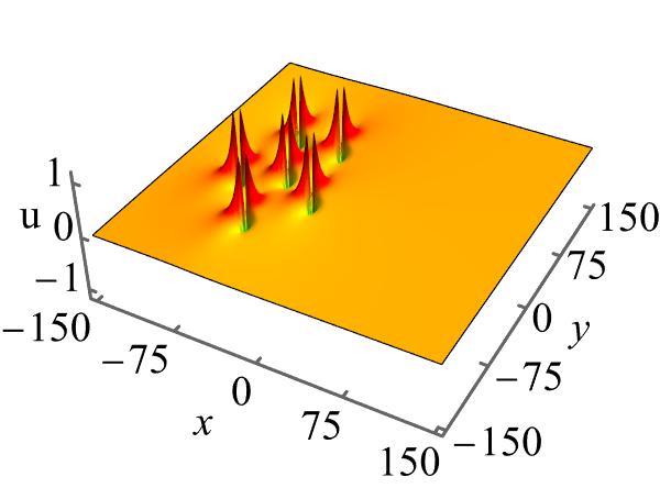
(a) $t=-25$

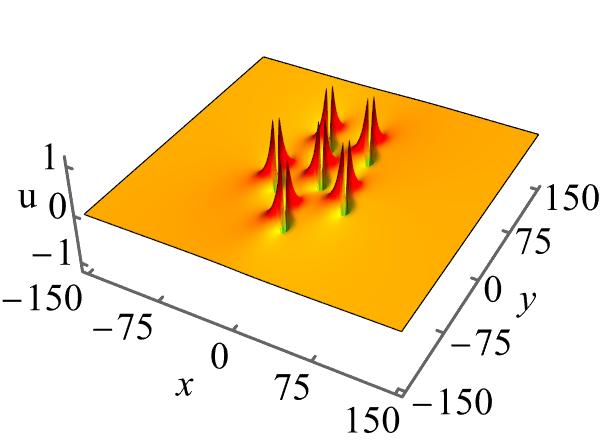
(b) $t=0$

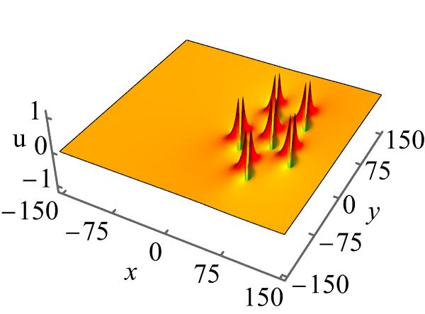
(c) $t=25$

Figure 3. The evolution of third-order lump-wave solution exhibiting a pentagon structure in the $x$–$y$ planes for $z=0.1$ at different time (a) $t=-25$, (b) $t=0$, and (c) $t=25$, with other parameters as $\gamma_{1}=-1;\ \gamma_{2}=-2;\ \mu=0.5;\ \beta_{1}=1;\ \beta_{2}=2;\ m=-0.2;\ n=0.5;\ \alpha_{3}=0.1;\ \alpha_{2}=-0.2;\ \beta_{3}=0.1;\ \gamma_{3}=0.3;\ \phi=0.5$; and $\psi=0.5.$

Based on the above analysis, one can extend the present procedure to construct the explicit form of the higher-order lump-wave solution of arbitrary order $n$ using the generalized polynomial function and their evolutionary dynamics can be explored in detail. The present analysis exposes the formation of different geometrical structures at various orders of the solutions, which resemble the studies reported in the literature for standard and extended KP-type nonlinear equations. As a future study, other types of localized wave solutions, such as solitons, breathers, and so on, can be constructed, and their characteristic dynamics can be explored in detail.

4. Conclusion

To summarize the present work, we have investigated a generalized (3+1)-dimensional nonlinearity-managed spatial symmetric dispersive model for higher-order lump-waves. By employing the Hirota bilinear method in conjunction with generalized polynomial expansions, we have constructed first-, second-, and third-order lump-wave solutions explicitly and generalized the results for arbitrary $n$-th order solutions. Our analysis of the obtained solutions reveals that the lump waves possess paired peaks with non-interacting behavior and exhibit different geometrical patterns/shapes, namely simple, triangular, and pentagonal structures with single, triple, and sextuple paired peaks, admitting manipulating possibilities using the available arbitrary parameters. The observations can provide valuable insights into the dynamics of higher-order lump structures in higher-dimensional water wave models and other diverse physical systems.

Acknowledgement

KM would like to thank SRM TRP Engineering College, India, for their financial support (Grant No. SRM/TRP/RI/005). KM is also supported by the Anusandhan National Research Foundation (ANRF), India — formerly known as the Science and Engineering Research Board (SERB), Government of India — through the MATRICS Research Grant (No. MTR/2023/000921).

References

- [CD17] Peter A Clarkson and Ellen Dowie, Rational solutions of the Boussinesq equation and applications to rogue waves, Trans. Math. Appl. 1 (2017), no. 1, tnx003.
- [GHLM21] Jutong Guo, Jingsong He, Maohua Li, and Dumitru Mihalache, Multiple-order line rogue wave solutions of extended Kadomtsev–Petviashvili equation, Math. Comput. Simul. 180 (2021), 251–257.
- [Hir04] Ryogo Hirota, The direct method in soliton theory (Cambridge University Press, Cambridge, 2004).
- [Kan25] Zhou-Zheng Kang, Searching for multiwave interaction solutions for a spatial symmetric generalized KP model in (2+ 1)-dimensions, Rom. J. Phys. 70 (2025), no. 3-4, 107.
- [Ma23] Wen-Xiu Ma, Lump waves in a spatial symmetric nonlinear dispersive wave model in (2+ 1)-dimensions, Math. 11 (2023), no. 22, 4664.
- [Ma24] WX Ma, Lump waves and their dynamics of a spatial symmetric generalized KP model, Rom. Rep. Phys 76 (2024), no. 3, 108.
- [MBA21] Wen-Xiu Ma, Yushan Bai, and Alle Adjiri, Nonlinearity-managed lump waves in a spatial symmetric HSI model, Eur. Phys. J. Plus 136 (2021), no. 2, 240.
- [MBM23] Wen-Xiu Ma, Sumayah Batwa, and Solomon Manukure, Dispersion-managed lump waves in a spatial symmetric KP model, East Asian J. Appl. Math. 13 (2023), no. 2, 246–256.
- [Pen21] Li-Juan Peng, Different wave structures for the completely generalized Hirota–Satsuma–Ito equation, Nonlinear Dyn. 105 (2021), no. 1, 707–716.
- [Yan10] Jianke Yang, Nonlinear waves in integrable and nonintegrable systems (SIAM, Philadelphia, 2010).
- [Zha18] Zhaqilao, A symbolic computation approach to constructing rogue waves with a controllable center in the nonlinear systems, Comput. Math. Appl. 75 (2018), no. 9, 3331–3342.
- [ZMM+24] Qunyan Zou, Jalil Manafian, Somaye Malmir, KH Mahmoud, A SA Alsubaie, Nilofer Ali Ewadh, and Ihssan Alrekabi, Exact breather waves solutions in a spatial symmetric nonlinear dispersive wave model in (2+ 1)-dimensions, Sci. Rep. 14 (2024), no. 1, 31718.