Quantum phase transitions and information-theoretic measures
of a spin-oscillator system with non-Hermitian coupling

Abstract

In this paper, we describe some interesting properties of a spin-oscillator system with non-Hermitian coupling. As shown earlier, the Hilbert space of this problem can be described by infinitely-many closed two-dimensional invariant subspaces together with the global ground state. We expose the appearance of exceptional points (EP) on such two-dimensional subspaces together with quantum phase transitions marking the transit from real to complex eigenvalues. We analytically compute some information-theoretic measures for this intriguing system, namely, the thermal entropy as well as the von Neumann and Rényi entropies using the framework of the so-called $G$-inner product. Such entropic measures are verified to be non-analytic at the points which mark the quantum phase transitions on the space of parameters – a naive comparison with Ehrenfest’s classification of phase transitions then suggests that these transitions are of the first order as the first derivatives of the entropies are discontinuous across such transitions.

I Introduction

Since nearly three decades, there has been a great interest in certain quantum systems dictated by non-Hermitian Hamiltonians that admit a real spectrum. Such studies became highly popular since the late 90s when it was discovered that systems respecting symmetry under the joint action of parity ($\mathcal{P}$) and time-reversal ($\mathcal{T}$) admit a real spectrum Bender and Boettcher (1998); Bender et al. (1999). It is now understood that a consistent quantum theory with an all-real spectrum, unitary time evolution, and a probabilistic interpretation for $\mathcal{PT}$-symmetric non-Hermitian systems can be developed in a modified Hilbert space equipped with a positive-definite ‘$\mathcal{CPT}$’-inner product Bender et al. (2002); Bender (2007); Mostafazadeh (2010), where $\mathcal{C}$ is an additional symmetry associated with all $\mathcal{PT}$-symmetric systems. Such a description, however, shall fail should $\mathcal{PT}$-symmetry be broken, in which case complex-conjugate eigenvalues appear in the spectrum. On the parameter space of the system, the breaking of $\mathcal{PT}$-symmetry Khare and Mandal (2000, 2009); Mandal et al. (2013, 2015); Raval and Mandal (2019); Mandal (2021); Modak and Mandal (2021); Pal et al. (2025); Ghatak et al. (2013) may be regarded as a quantum phase transition – the two phases, namely, the $\mathcal{PT}$-symmetric phase and the $\mathcal{PT}$-broken phase are separated by the so-called EP. $\mathcal{PT}$-symmetric non-Hermitian systems have found numerous applications in various branches of physics and interdisciplinary areas Hasan and Mandal (2018); Hasan et al. (2020); Basu-Mallick and Mandal (2001); Basu-Mallick et al. (2004); Bender et al. (2013); Mandal and Ghatak (2012); Ghatak et al. (2015); Hajong et al. (2024); Dwivedi and Mandal (2021); Hasan and Mandal (2020a); Banerjee et al. (2024); Bhowmick et al. (2025); Hasan and Mandal (2020b); Hajong et al. (2025); Brihaye et al. (2007); Mandal and Gupta (2010); Kumari et al. (2016).

It has subsequently been realized that although $\mathcal{PT}$-symmetry is a sufficient condition for the reality of the spectrum of a non-Hermitian Hamiltonian, it is not necessary Mostafazadeh (2010). $\mathcal{PT}$-symmetric non-Hermitian systems are only a subset of a bigger class of non-Hermitian systems, known as pseudo-Hermitian system, defined as Mostafazadeh (2010)

$$H=G^{-1}H^{\dagger}G,\quad\quad G^{\dagger}=G.$$ (1)

That is, the Hamiltonian and its Hermitian conjugate are related by a similarity transformation; if $G$ is the identity operator, then $H=H^{\dagger}$, i.e., the Hamiltonian equals its Hermitian conjugate. A Hamiltonian admitting the condition (1) may or may not be $\mathcal{PT}$-symmetric. However, it can be shown that the condition (1) naturally implies that the Hamiltonian is symmetric under the action of a linear ($L$) and an antilinear ($A$) operator, i.e., $[H,L]=0=[H,A]$. These operators $L$ and $A$ correspond to $\mathcal{P}$ and $\mathcal{T}$ operators in case of $\mathcal{PT}$ symmetric systems Mostafazadeh (2002a). Consequently, it has been shown that such systems admitting complete real spectrum when the operator $G$ is positive definite. It was natural to modify the Hilbert space by introducing G-inner product:

$$(\psi,\phi)_{G}\equiv\langle\psi|G|\phi\rangle.$$ (2)

to have a consistent quantum theory with pseudo-Hermitian systems. Note that $G=\mathcal{CPT}$ is only a special case. Now, given the time-evolution operator $e^{iHt}$ (we will adopt units in which $\hbar=1$), one can write

$$\langle\psi(t)|G|\phi(t)\rangle = \langle\psi(0)|e^{iH^{\dagger}t}Ge^{-iHt}|\phi(0)\rangle$$

$$= \langle\psi(0)|G(G^{-1}e^{iH^{\dagger}t}G)e^{-iHt}|\phi(0)\rangle$$

$$= \langle\psi(0)|G|\phi(0)\rangle,$$ (4)

where in the last step, we used the condition (1). The above result shows that the time evolution is unitary with respect to the modified inner product that possesses the metric $G$; because we have imposed $G$ to be positive definite, the norms of the states are positive which allows for a consistent quantum mechanical interpretation. We refer the reader to Mostafazadeh (2002b); Kretschmer and Szymanowski (2004); Ghatak and Mandal (2013) for more details on pseudo-Hermitian quantum systems.

As with $\mathcal{PT}$-symmetric systems exhibiting the breaking of $\mathcal{PT}$-symmetry at quantum phase transitions, one can encounter phase transitions in pseudo-Hermitian (but not necessarily $\mathcal{PT}$-symmetric) systems as well. On the parameter space, this happens at the EP which are singular points at which two or more eigenstates (eigenvalues and eigenvectors) coalesce. Referring to the condition (1), the metric operator $G$ exhibits non-invertibility at the EP, leading to the notion of self-orthogonality (vanishing of norm) which has interesting physical consequences such as the stopping of light in optical systems Goldzak et al. (2018). Moreover, in the so-called ‘pseudo-Hermiticity-broken’ phase where complex eigenvalues appear, $G$ becomes time-dependent, and at the EP, $G$ is singular. However, even in the pseudo-Hermiticity-broken phase, it is possible to associate a metric $G$, which, however does not satisfy Eq. (1). As a result, the eigenvalues are complex and the time-evolution is non-unitary despite being able to define inner products consistently.

One of the aims of this work is to study such quantum phase transitions in a pseudo-Hermitian but non-$\mathcal{PT}$-symmetric system, with the aid of the $G$-inner product. Further, it can be observed that although the study of pseudo-Hermitian (especially, $\mathcal{PT}$-symmetric) systems has gained considerable popularity over the past decades, there have been a relatively less number of developments devoted to the study of information-theoretic aspects such as density matrices and entropies (see Sinha et al. (2024); Bagarello et al. (2025); Fring and Frith (2019); Wehrl (1978); Casini and Huerta (2009); Rényi (1961) and references therein). Thus, with this in mind, one of the other aims of the present work is to study such quantities in the light of the quantum phase transitions mentioned above. In particular, we will present results on the Boltzmann, von Neumann, and Rényi entropies using the framework of the $G$-inner product and study their behavior across the EP marking the boundary between the pseudo-Hermitian and ‘pseudo-Hermiticity broken’ phases. The system that we are picking consists of a spin that is interacting with a bosonic oscillator with a non-Hermitian coupling, a model that has been explored earlier in Mandal (2005). Intriguingly, the Hilbert space of this problem can be described by infinitely many two-dimensional subspaces that are ‘closed’, together with the global ground state Mandal (2005). As we shall show, each of the above-mentioned two-dimensional invariant subspaces of the Hilbert space admits its own EP and quantum phase transition although the qualitative behavior of the attributes remains similar across different subspaces, which are infinite in number. Both the thermodynamic as well as quantum entropies have abrupt changes at the EP in each invariant subspace and the first derivative of the entropies suffer discontinuity at the EP leading to a first order phase transition.

II The Model

The system of interest is a spin-1/2 particle in an external magnetic field $\bm{B}$, coupled to an oscillator through some non-Hermitian interaction Mandal (2005). The Hamiltonian reads

$$H=\mu\bm{\sigma}.{\bf B}+\hbar\omega a^{\dagger}a+\gamma(\sigma_{+}a-\sigma_{-}a^{\dagger}),$$ (5)

where $\sigma$’s are the Pauli matrices, $\gamma$ is some real parameter for non-Hermitian interaction , $\sigma_{\pm}\equiv\frac{1}{2}[\sigma_{x}\pm\iota\sigma_{y}]$ are spin-projection operators, while $a$, $a^{\dagger}$ are the usual creation and annihilation operators for the oscillator states defined as

$$a=\frac{p-im\omega x}{\sqrt{2m\omega\hbar}},\quad\quad a^{\dagger}=\frac{p+im\omega x}{\sqrt{2m\omega\hbar}},$$ (6)

with

$$a|n\rangle=\sqrt{n}|n-1\rangle\quad{\rm and}\quad{}a^{\dagger}|n\rangle=\sqrt{n+1}|n+1\rangle,$$ (7)

where the notation $|n\rangle$ for the energy eigenstates for the oscillator has been adopted.

For the sake of simplicity, we choose the external magnetic field to be in $z$-direction, i.e., ${\bf B}=B_{o}\hat{z}$ and the Hamiltonian for the system in Eq. (5) is reduced to

$$H=\frac{\epsilon}{2}\sigma_{z}+\hbar\omega a^{\dagger}a+\gamma(\sigma_{+}a-\sigma_{-}a^{\dagger}),$$ (8)

where $\epsilon=2\mu B_{o}$. This system can also be thought of as a two-level system coupled to an oscillator where $\epsilon$ is the spacing between the levels. Note that this Hamiltonian is not Hermitian as

$$H^{\dagger}=\frac{\epsilon}{2}\sigma_{z}+\hbar\omega a^{\dagger}a-\gamma(\sigma_{+}a-\sigma_{-}a^{\dagger})\neq H,$$ (9)

since $\sigma_{\pm}^{\dagger}=\sigma_{\mp}$.

II.1 Pseudo-Hermiticity

Now, under the parity transformation $\mathcal{P}$, i.e., $x\rightarrow-x,p\rightarrow-p$, both $\bm{\sigma}$ and B remain invariant as both are axial vectors but the creation and annihilation operators slip their sign. Explicitly, we have

$$\mathcal{P}\bm{\sigma}\mathcal{P}^{-1} =\bm{\sigma},\qquad\mathcal{P}{\bf B}\mathcal{P}^{-1}={\bf B},$$ (10)

$$\mathcal{P}a^{\dagger}\mathcal{P}^{-1} =-a^{\dagger},\quad\mathcal{P}a\mathcal{P}^{-1}=-a.$$

The time-reversal operator for the system of spin-1/2 particles is $\mathcal{T}=-i\sigma_{y}K$ where $K$ is complex-conjugation operator. Let us note the changes of the following quantities under time-reversal transformation as follows,

$$\mathcal{T}\bm{\sigma}\mathcal{T}^{-1} =-\bm{\sigma},\quad\mathcal{T}{\bf B}\mathcal{T}^{-1}={\bf B},\quad\mathcal{T}\sigma_{\pm}\mathcal{T}^{-1}=-\sigma_{\mp},$$ (11)

$$\mathcal{T}a^{\dagger}\mathcal{T}^{-1} =-a^{\dagger},\quad\mathcal{T}a\mathcal{T}^{-1}=-a.$$

It must be remarked that we have considered the magnetic field as an external element in our system which does not change sign under time-reversal transformation. From Eqs. (10) and (11) we can see that the Hamiltonian in Eq. (8) is not $\mathcal{PT}$-symmetric as:

$$(\mathcal{PT})H(\mathcal{PT})^{-1} =-\frac{\epsilon}{2}\sigma_{z}+\hbar\omega a^{\dagger}a+\gamma(\sigma_{+}a-\sigma_{-}a^{\dagger})\neq H.$$ (12)

Nevertheless, the Hamiltonian is pseudo-Hermitian as it follows that:

$$\sigma_{z}H\sigma_{z}^{-1} =\frac{\epsilon}{2}\sigma_{z}+\hbar\omega a^{\dagger}a-\gamma(\sigma_{+}a-\sigma_{-}a^{\dagger})=H^{\dagger}.$$ (13)

Moreover, we can write:

$$\mathcal{P}H\mathcal{P}^{-1} =\frac{\epsilon}{2}\sigma_{z}+\hbar\omega a^{\dagger}a-\gamma(\sigma_{+}a-\sigma_{-}a^{\dagger})=H^{\dagger}.$$ (14)

Therefore, the Hamiltonian is invariant under the transformation generated by the combined operator $\mathcal{P}\sigma_{z}$, i.e., $[H,P\sigma_{z}]=0$. Comparing (13) and (14) with (1), one can easily conclude that $\sigma_{z}$ or $\mathcal{P}$ correspond to the $G$ operator mentioned therein. Note, however, that because these are not positive-definite, they cannot define a consistent inner product. However, as we shall demonstrate in section (III), it is possible to construct a metric $G$ which is positive definite, allowing one to define a consistent inner product.

II.2 Spectrum and eigenstates

To find the eigenvalues and the corresponding eigenvectors of the system described by the Hamiltonian in Eq. (5), we adopt the notation for a state as $\left|n,\frac{1}{2}m_{s}\right\rangle$, where $n$ is eigenvalue for the number operator $a^{\dagger}a$ and $m_{s}=\pm 1$ are the eigenvalues of the operator $\sigma_{z}$. It is readily seen that $\left|0,-\frac{1}{2}\right\rangle$ is the global ground state of the Hamiltonian with eigenvalue $-\frac{\epsilon}{2}$ and it is non-degenerate, i.e.,

$$H\left|0,-\frac{1}{2}\right\rangle=-\frac{\epsilon}{2}\left|0,-\frac{1}{2}\right\rangle.$$ (15)

It is easy to check that the next possible state $\left|0,\frac{1}{2}\right\rangle$ is not an eigenstate of the Hamiltonian. However, this state along with the state $\left|1,-\frac{1}{2}\right\rangle$ close under the action of the Hamiltonian and form an invariant subspace in the space of states which can be seen as follows:

$$H\left|0,\frac{1}{2}\right\rangle=\frac{\epsilon}{2}\left|0,\frac{1}{2}\right\rangle-\gamma\left|1,-\frac{1}{2}\right\rangle,$$ (16)

$$H\left|1,-\frac{1}{2}\right\rangle=\left(\hbar\omega-\frac{\epsilon}{2}\right)\left|1,-\frac{1}{2}\right\rangle+\gamma\left|0,\frac{1}{2}\right\rangle.$$

Thus, the first two excited states belong to this two-dimensional sector; the matrix Hamiltonian acting on this subspace can be written in the matrix form as

$$H_{1}=\begin{pmatrix}\frac{\epsilon}{2}&\gamma\\ -\gamma&-\frac{\epsilon}{2}+\hbar\omega\end{pmatrix}.$$ (17)

The eigenvalues of this Hamiltonian matrix are given by $R^{\rm I,II}_{1}=\frac{1}{2}[\hbar\omega\pm\sqrt{(\hbar\omega-\epsilon)^{2}-4\gamma^{2}}]$. The result is easily generalized to the sector spanned by $\left|n,\frac{1}{2}\right\rangle$ and $\left|n+1,-\frac{1}{2}\right\rangle$, wherein the Hamiltonian matrix is given by

$$H_{n+1}=\begin{pmatrix}\frac{\epsilon}{2}+n\hbar\omega&\gamma\sqrt{n+1}\\ -\gamma\sqrt{n+1}&-\frac{\epsilon}{2}+(n+1)\hbar\omega\end{pmatrix}.$$ (18)

The corresponding eigenvalues are

$$R^{\rm I,II}_{n+1}=\frac{1}{2}[(2n+1)\hbar\omega\pm\sqrt{(\hbar\omega-\epsilon)^{2}-4\gamma^{2}(n+1)}].$$ (19)

Next, let us have a look at the Hermitian conjugate of $H_{n+1}$ which goes as

$$H_{n+1}^{\dagger}=\begin{pmatrix}\frac{\epsilon}{2}+n\hbar\omega&-\gamma\sqrt{n+1}\\ \gamma\sqrt{n+1}&-\frac{\epsilon}{2}+(n+1)\hbar\omega\end{pmatrix}.$$ (20)

Let us denote eigenvalues of $H$ as $R^{\rm I}$ and $R^{\rm II}$, and eigenvalues of the Hamiltonian $H^{\dagger}$ as $L^{\rm I}$ and $L^{\rm II}$. Then, it can be readily seen that, for the $(n+1)^{th}$ subspace:

$$R^{\rm I,II}_{n+1}= L^{\rm I,II}_{n+1}=\frac{1}{2}[(2n+1)\hbar\omega\pm\sqrt{(\hbar\omega-\epsilon)^{2}-4\gamma^{2}(n+1)}].$$ (21)

Some comments are now in order. Clearly, the matrices $H_{n+1}$ for $n=0,1,\cdots$ are pseudo-Hermitian, exhibiting real eigenvalues if $(\hbar\omega-\epsilon)^{2}-4\gamma^{2}(n+1)>0$. The region of the parameter space in which the eigenvalues are real and distinct then corresponds to the region where pseudo-Hermiticity is unbroken, whereas for $(\hbar\omega-\epsilon)^{2}-4\gamma^{2}(n+1)<0$, the eigenvalues of each $H_{n+1}$ appear in complex-conjugate pairs indicating the pseudo-Hermiticity has been broken for such parameters and we cannot write for $H_{n+1}$ are relation akin to Eq. (1) for a Hermitian $G$. The two above-mentioned parameter regimes are connected by the curve $(\hbar\omega-\epsilon)^{2}-4\gamma^{2}(n+1)=0$ on the $\gamma-\epsilon$ parameter space for a given $n$. For parameter values on this curve, one essentially gets a single eigenvalue of $H_{n+1}$ but what is more intriguing is that these are not mere degeneracies but singular points named ‘EPs’ at which the eigenvectors also coalesce. Therefore, to summarize, the regions of unbroken and broken pseudo-Hermiticity are obtained as

$$|\hbar\omega-\epsilon|\geq 2\gamma\sqrt{n+1}~~\text{(unbroken region)},$$ (22a)

$$|\hbar\omega-\epsilon|<2\gamma\sqrt{n+1}~~\text{(broken region)}.$$ (22b)

while EP satisfy

$$\gamma_{n+1}^{c}=\frac{|\hbar\omega-\epsilon|}{2\sqrt{n+1}},$$ (23)

for the $n^{\rm th}$ subspace. In the above, the superscript ‘c’ on $\gamma$ indicates the value for which with a given $n$ and $\epsilon$, one hits an EP. The transition between the unbroken and broken regions of pseudo-Hermiticity through the EP can be understood as a quantum phase transition. In Fig. (1), we have plotted the equation $(\hbar\omega-\epsilon)^{2}-4\gamma^{2}(n+1)=0$, obtained by setting to zero the discriminant appearing in the roots appearing in Eq. (21) for $n=0,1,2,3$. The regions shaded in red correspond to negative values of the discriminant giving rise to eigenvalues of $H_{n+1}$ that are complex conjugates. On the other hand, the regions shaded in green correspond to positive values of the discriminant giving rise to real and distinct eigenvalues of $H_{n+1}$. These two regions therefore correspond to the pseudo-Hermiticity-broken and pseudo-Hermiticity-unbroken phases, respectively, with the lines separating them (discriminant = 0) corresponding to the EP on the $\epsilon$$\gamma$-parameter space. In what follows, we will explore this kind of phase transition in some detail. Henceforth we adopt the short terms ‘unbroken’ and ‘broken’ phases in the places of ‘pseudo-Hermiticity-unbroken’ and ‘pseudo-Hermiticity-broken’ phases, respectively for brevity.

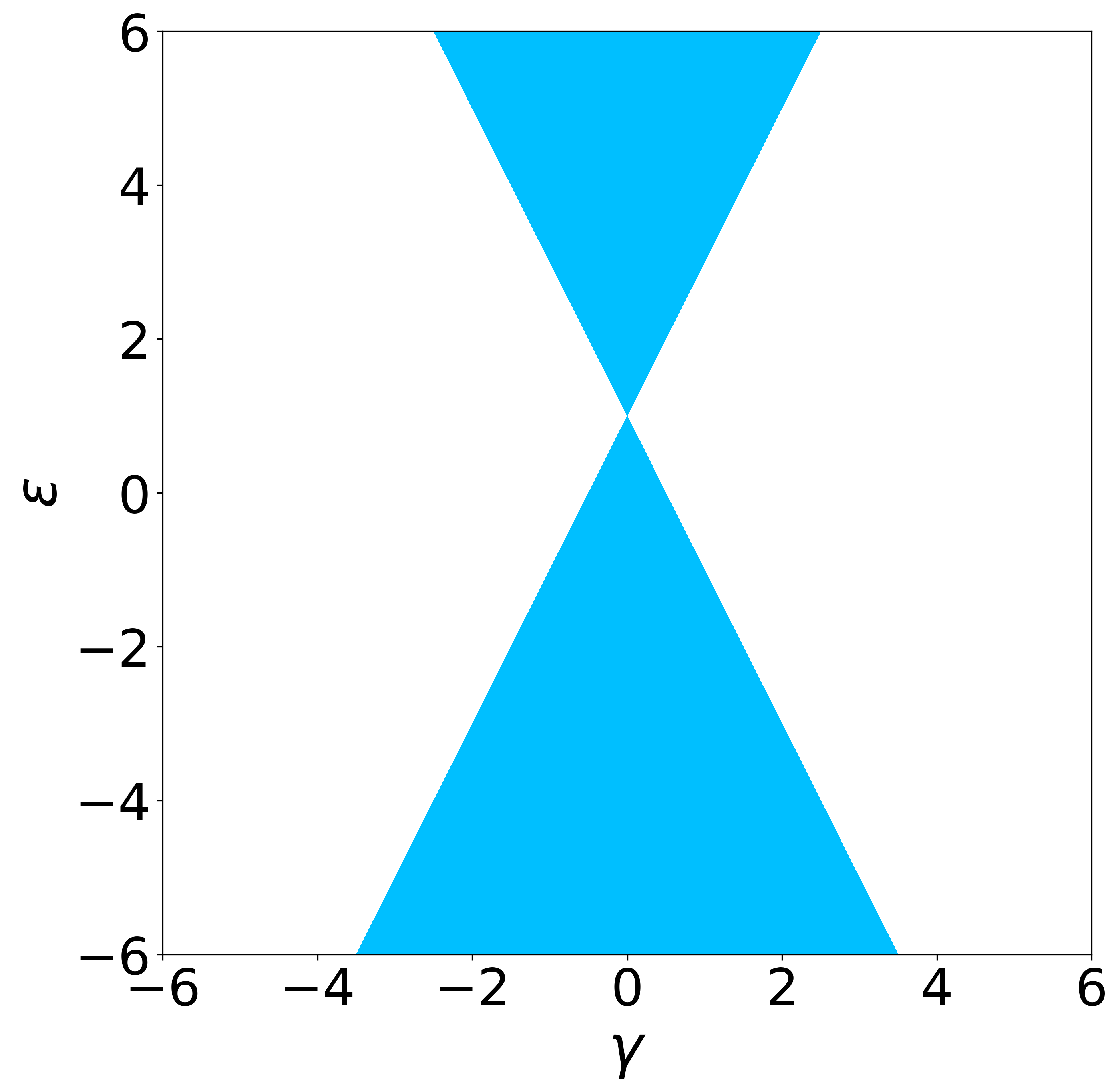
(a)  $n=0$

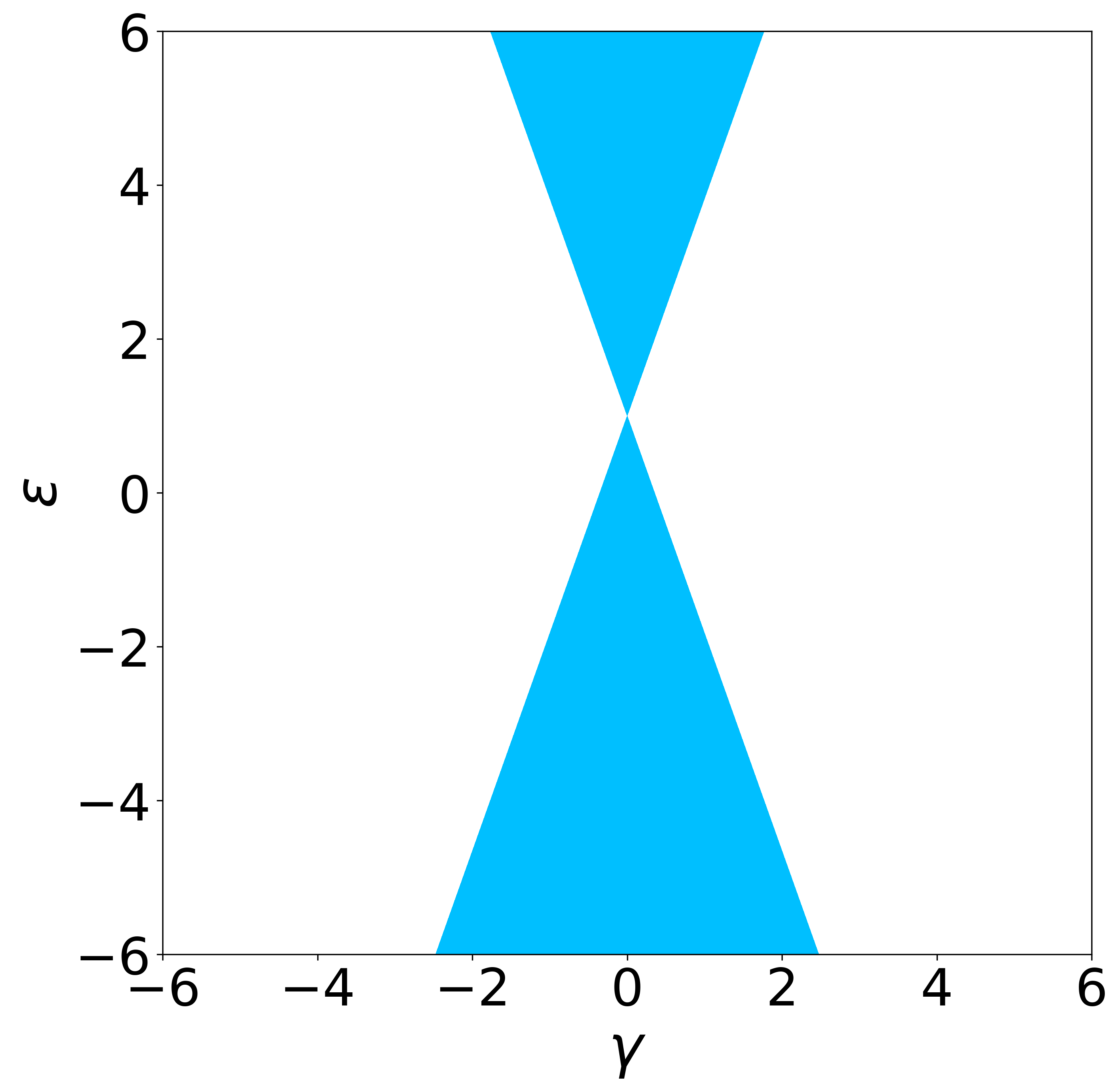
(b)  $n=1$

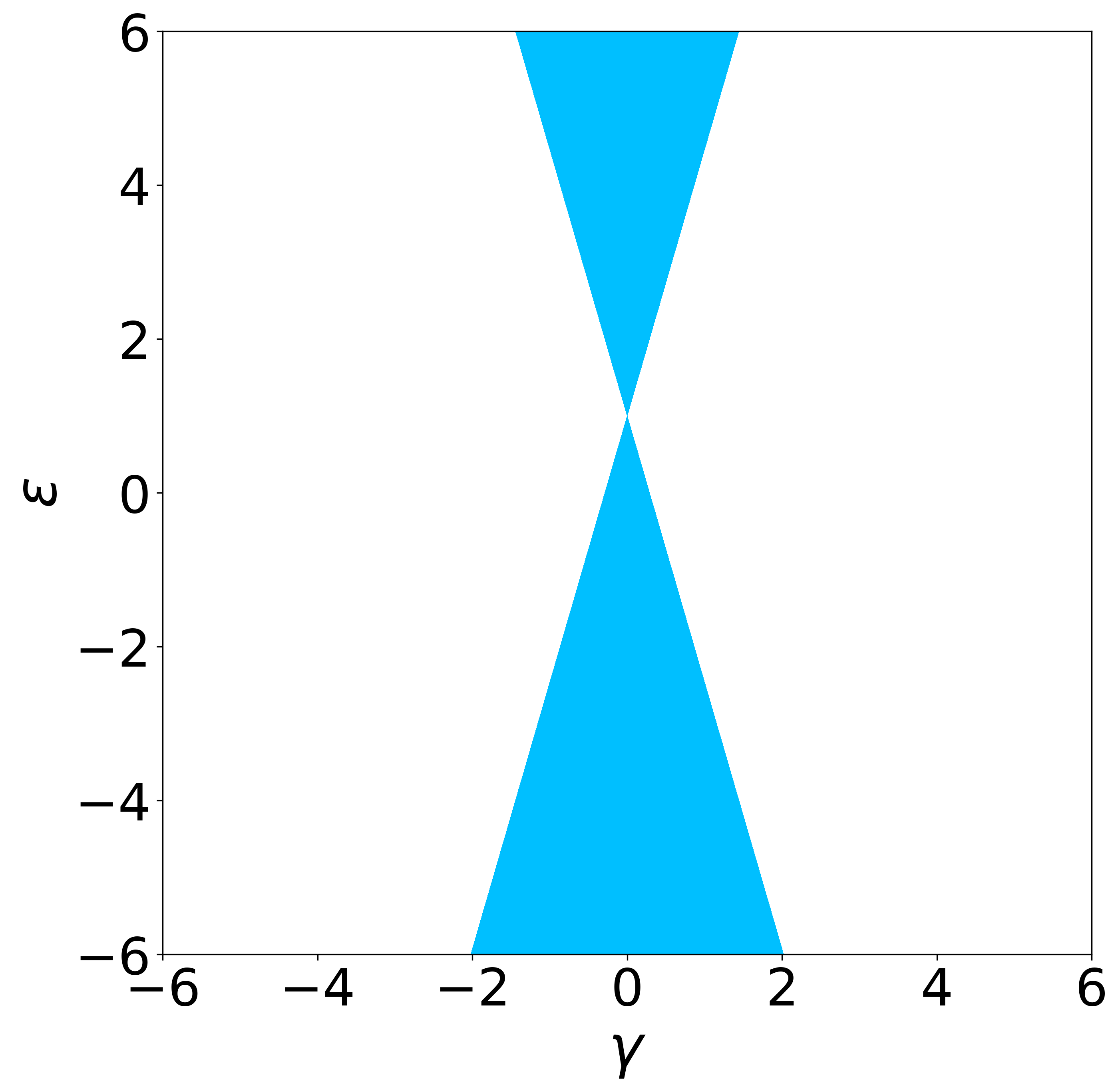
(c)  $n=2$

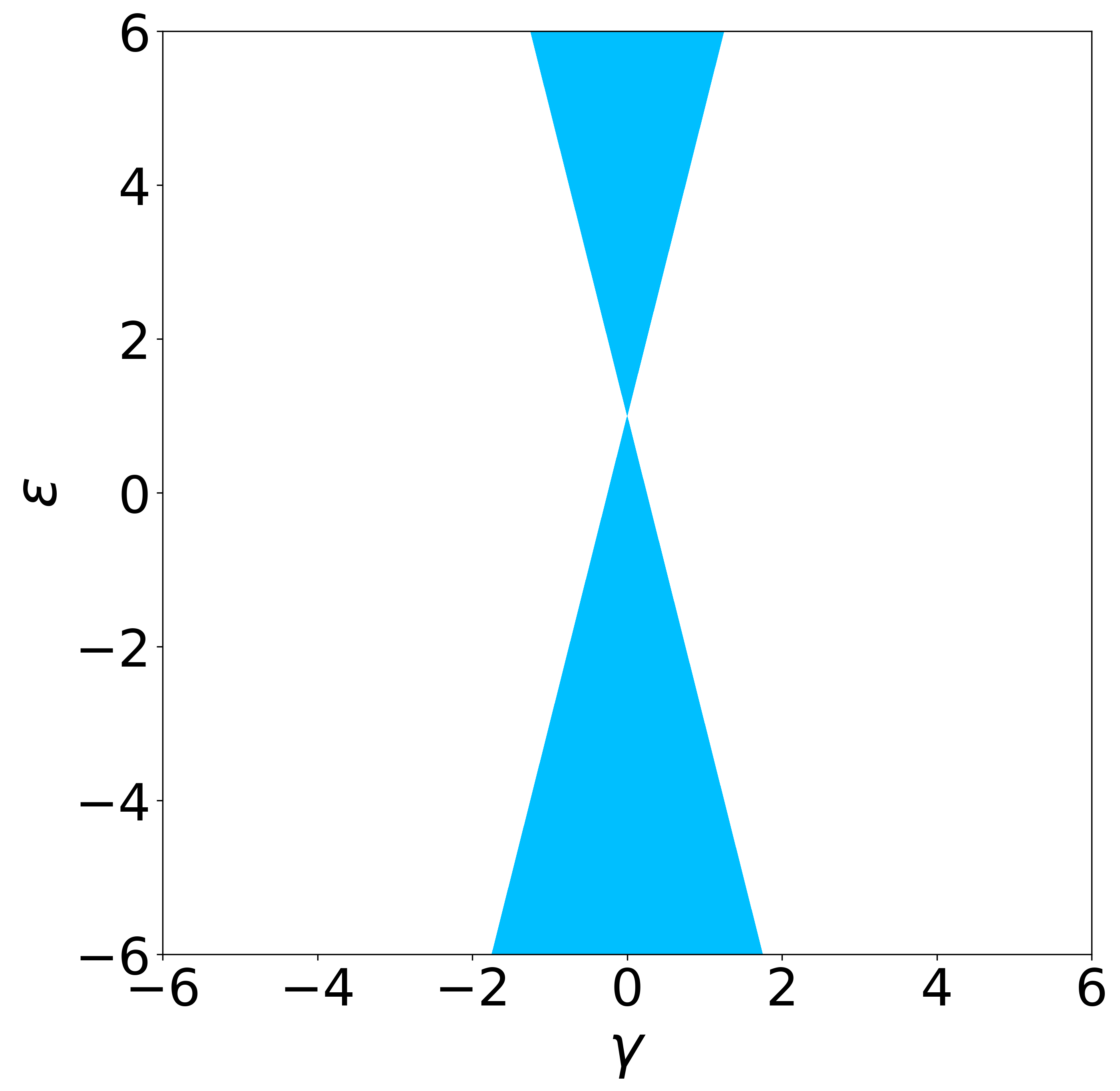
(d)  $n=3$

Figure 1: Figures showing the regions of the $\epsilon$$\gamma$-parameter space in which pseudo-Hermiticity is broken (unshaded) and unbroken (shaded) for $n=0,1,2,3$. EP lie on the lines separating the two regions.

III The $G$-inner product

For a non-Hermitian Hamiltonian $H$, there are distinct left and right eigenvectors $\left\langle L_{m}\right|$ and $\left|R_{m}\right\rangle$, respectively. In the bi-orthogonal interpretation of quantum mechanics Brody (2013), the inner product is defined as $\left\langle L_{m_{1}}|R_{m_{2}}\right\rangle=\delta_{m_{1},m_{2}}$. The metric $G$ can always be chosen as (except for at the EP) Hajong et al. (2024); Shukla et al. (2023); Ju et al. (2019); Tzeng et al. (2021)

$$G\equiv\sum_{m}\left|L_{m}\right\rangle\left\langle L_{m}\right|,$$ (24)

where $\left|L_{m}\right\rangle$ are the eigenstates of $H^{\dagger}$,

$$H|R_{m}\rangle=R_{m}|R_{m}\rangle\,,\quad H^{\dagger}|L_{m}\rangle=L_{m}|L_{m}\rangle\,.$$ (25)

The inner product may now be defined as

$$\left\langle R_{m_{1}}\right|\mathcal{O}\left|R_{m_{2}}\right\rangle_{G}\equiv\left\langle R_{m_{1}}\right|G\mathcal{O}\left|R_{m_{2}}\right\rangle,$$ (26)

where $\mathcal{O}$ is some observable. Substituting Eq. (24), one immediately obtains

$$\left\langle R_{m_{1}}\right|\mathcal{O}\left|R_{m_{2}}\right\rangle_{G}=\left\langle L_{m_{1}}\right|\mathcal{O}\left|R_{m_{2}}\right\rangle,$$ (27)

where we notice that the bi-orthogonal inner product appears naturally. Moreover, notice that we have not made use of the condition given in Eq. (1), i.e., the above-mentioned prescription of constructing the metric operator can be extended to the region where Eq. (1) does not hold which is the region with broken pseudo-Hermiticity. Thus, with the understanding that the metric operator can be constructed using the general prescription given in Eq. (24), we will proceed on to studying the two phases mentioned earlier.

III.1 Unbroken region

In this region, the condition given in Eq. (22a) is met and the eigenvalues $R^{\rm I,II}=L^{\rm I,II}$ are real and distinct. Let us find the normalized eigenvectors of the matrix $H_{n+1}$. In particular, keeping in mind that a non-Hermitian matrix admits distinct left and right eigenvectors, will use the notations

$${\rm Right~eigenvectors}:\ |R^{\rm I}_{n+1}\rangle=-\frac{1}{\sqrt{1-(\Phi^{\rm I})^{2}}}\begin{pmatrix}1\\ \Phi^{\rm I}\end{pmatrix},$$ (28)

$$|R^{\rm II}_{n+1}\rangle=\frac{1}{\sqrt{(\Phi^{\rm II})^{2}-1}}\begin{pmatrix}-1\\ \Phi^{\rm II}\end{pmatrix},$$

$${\rm Left~eigenvectors}:\ |L^{\rm I}_{n+1}\rangle=\frac{1}{\sqrt{1-(\Phi^{\rm I})^{2}}}\begin{pmatrix}-1\\ \Phi^{\rm I}\end{pmatrix},$$

$$|L^{\rm II}_{n+1}\rangle=\frac{1}{\sqrt{(\Phi^{\rm II})^{2}-1}}\begin{pmatrix}1\\ \Phi^{\rm II}\end{pmatrix},$$

where $\Phi^{\rm I,II}=\frac{\delta}{\sqrt{4-\delta^{2}}\mp 2}$ and $\delta=\sqrt{(1+n)}\gamma$.
For definiteness, henceforth, we set the parameters $\hbar=\omega=1,\epsilon=5$. Now, in the $(n+1)^{\rm th}$ subspace, one can calculate the $G$-matrix in order to define the inner product as described earlier. The metric turns out to be

$$G_{n+1}= \sum_{i={\rm I,II}}|L^{i}_{n+1}\rangle\langle L^{i}_{n+1}|=\frac{1}{\sqrt{4-\delta^{2}}}\begin{pmatrix}2&\delta\\ \delta&2\end{pmatrix}.$$ (29)

On computing the $G$-inner product, the modified Hamiltonian matrix $H_{n+1}$ in the $(n+1)^{th}$ subspace takes the following appearance (using Eqs. (18) and (29)) :

$$H^{G}_{n+1}=\begin{pmatrix}\frac{(2n+1)+(4-\delta^{2})}{\sqrt{4-\delta^{2}}}&\frac{(2n+1)\delta}{2\sqrt{4-\delta^{2}}}\\ \frac{(2n+1)\delta}{2\sqrt{4-\delta^{2}}}&\frac{(2n+1)-(4-\delta^{2})}{\sqrt{4-\delta^{2}}}\end{pmatrix},$$ (30)

where the matrix elements are obtained via the $G$-inner product. The matrix $H^{G}_{n+1}$ is Hermitian as expected and we will denote the eigenvalues and normalized eigenvectors of this matrix as

$$\lambda^{\rm I,II}_{n+1} = \frac{2(2n+1)\pm\sqrt{(2n+1)^{2}\delta^{2}+4(4-\delta^{2})^{2}}}{2\sqrt{4-\delta^{2}}}\,,$$ (31)

$$\left|\lambda^{\rm I,II}_{n+1}\right\rangle = \begin{pmatrix}\frac{\Theta^{\rm I,II}}{\sqrt{1+({\Theta^{\rm I,II}})^{2}}}\\ \,\\ \frac{1}{\sqrt{1+({\Theta^{\rm I,II}})^{2}}}\end{pmatrix}\,,$$ (32)

with

$$\Theta^{\rm I,II} = \frac{2(4-\delta^{2})\pm\sqrt{(2n+1)^{2}\delta^{2}+4(4-\delta^{2})^{2}}}{(2n+1)\delta}\,.$$ (33)

III.2 Broken region

In the region where pseudo-Hermiticity is broken using Eq. (22b), let us adopt the following notation for the right and left eigenvectors and calculate them:

$${\rm Right~eigenvectors}:\ |\tilde{R}^{\rm I}_{n+1}\rangle=\frac{1}{\sqrt{(\tilde{\Phi}^{\rm I})^{2}-1}}\begin{pmatrix}1\\ \tilde{\Phi}^{\rm I}\end{pmatrix},$$ (34)

$$|\tilde{R}^{\rm II}_{n+1}\rangle=\frac{1}{\sqrt{(\tilde{\Phi}^{\rm II})^{2}-1}}\begin{pmatrix}-1\\ \tilde{\Phi}^{\rm II}\end{pmatrix},$$

$${\rm Left~eigenvectors}:\ |\tilde{L}^{\rm II}_{n+1}\rangle=\frac{1}{\sqrt{(\tilde{\Phi}^{\rm II})^{2}-1}}\begin{pmatrix}1\\ \tilde{\Phi}^{\rm II}\end{pmatrix},$$

$$|\tilde{L}^{\rm II}_{n+1}\rangle=\frac{1}{\sqrt{(\tilde{\Phi}^{\rm I})^{2}-1}}\begin{pmatrix}-1\\ \tilde{\Phi}^{\rm I}\end{pmatrix},$$

where $\tilde{\Phi}^{\rm I,II}=\frac{\delta}{\iota\sqrt{\delta^{2}-4}\mp 2}$.

Henceforth, we adopt the convention that the symbol with ’tilde’ represents broken phase. The metric is then calculated from Eq. (24) as

$$\tilde{G}_{n+1}= \sum_{i={\rm I,II}}|\tilde{L}^{i}_{n+1}\rangle\langle\tilde{L}^{i}_{n+1}|=\frac{1}{\sqrt{\delta^{2}-4}}\begin{pmatrix}\delta&2\\ 2&\delta\end{pmatrix},$$ (35)

On computing the $G$-inner product in the broken region, the modified Hamiltonian matrix $H_{n+1}$ in the $(n+1)^{th}$ subspace takes the following appearance (using Eqs. (18) and (35)) :

$$\tilde{H}^{G}_{n+1}=\begin{pmatrix}\frac{(2n+1)\delta}{2\sqrt{\delta^{2}-4}}&\frac{(2n+1)-(\delta^{2}-4)}{\sqrt{\delta^{2}-4}}\\ \frac{(2n+1)+(\delta^{2}-4)}{\sqrt{\delta^{2}-4}}&\frac{(2n+1)\delta}{2\sqrt{\delta^{2}-4}}\end{pmatrix},$$ (36)

which is clearly non-Hermitian as anticipated, hence the eigenvalues are complex.

$$\tilde{\lambda}^{\rm I,II}_{n+1} = \frac{(2n+1)\delta\pm 2\sqrt{(2n+1)^{2}-(\delta^{2}-4)^{2}}}{2\sqrt{\delta^{2}-4}}$$ (37)

$$\left|\tilde{\lambda}^{\rm I,II}_{n+1}\right\rangle = \frac{1}{\sqrt{2}}\begin{pmatrix}\tilde{\Theta}^{\rm I,II}\\ 1\end{pmatrix}\,,$$ (38)

with

$$\tilde{\Theta}^{\rm I,II}=\pm\sqrt{\frac{(2n+1)-(\delta^{2}-4)}{(2n+1)+(\delta^{2}-4)}}$$ (39)

These results will be used in later sections to compute the entropies.

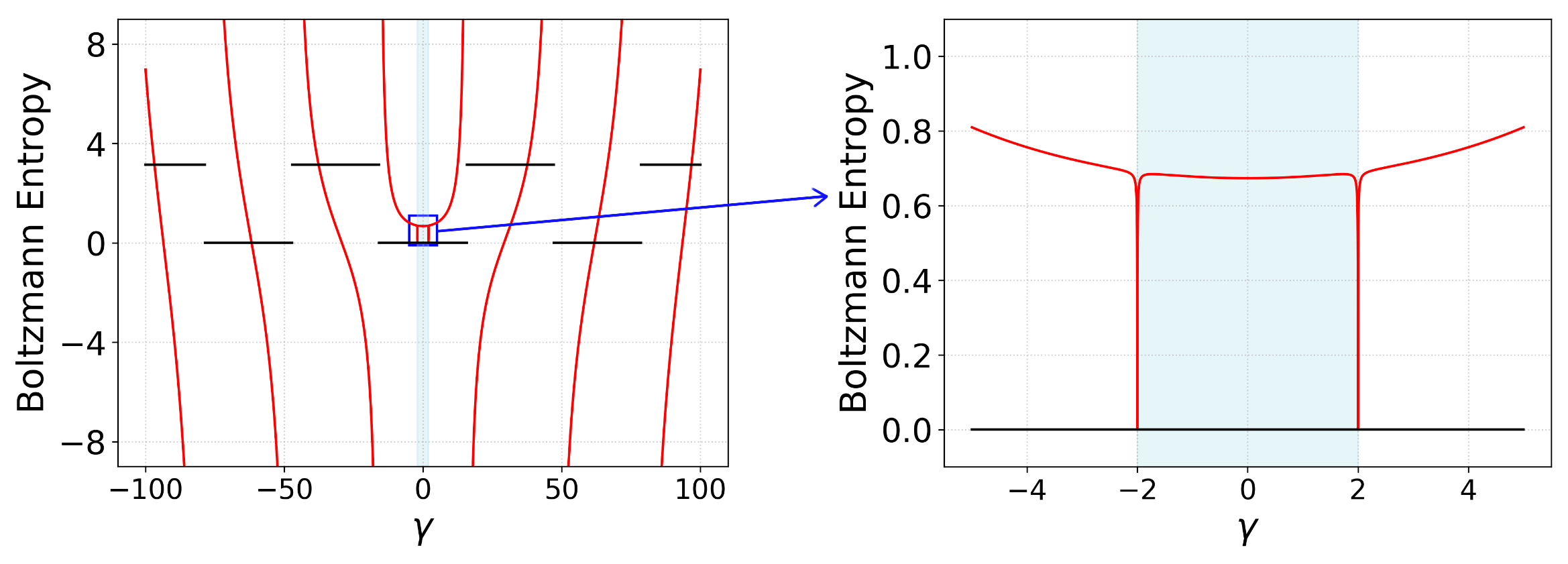
(a)  $n=0$

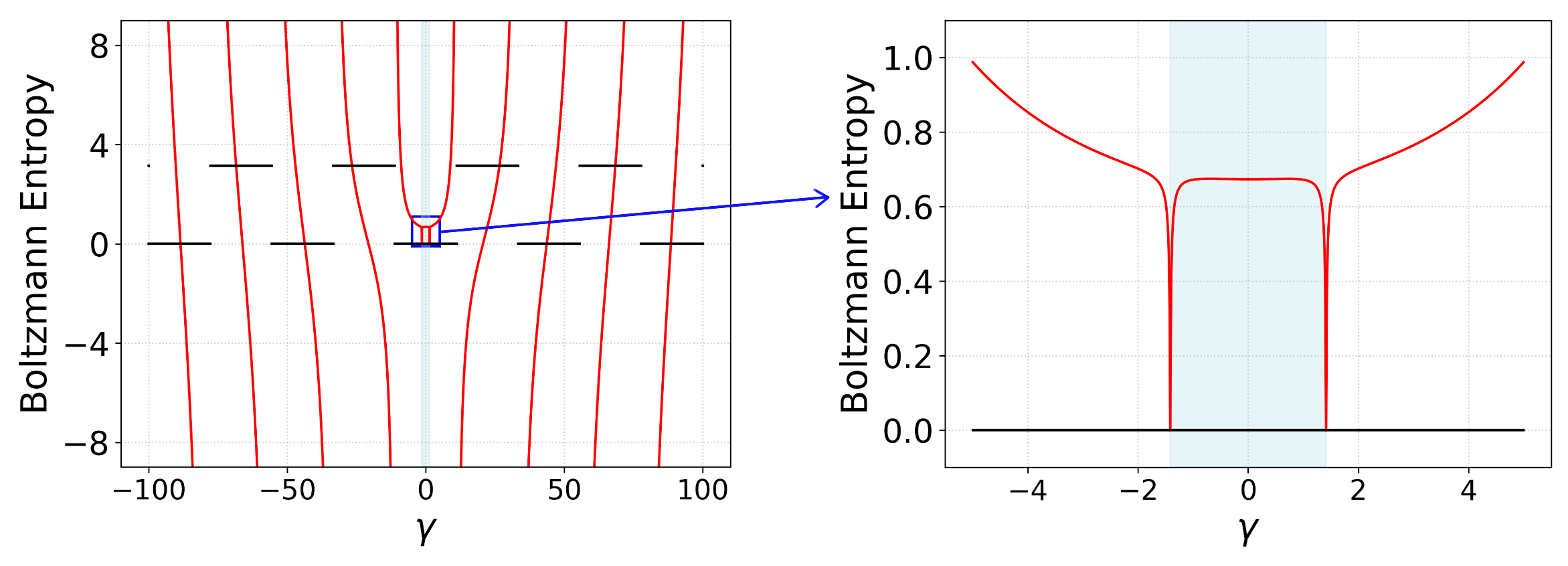
(b)  $n=1$

Figure 2: Variation of the Boltzmann entropy as a function of the parameter $\gamma$ for $n=0,1$. Red lines denote real part of Boltzmann entropy while the black lines denote its imaginary part. The shaded (blue) region denotes the unbroken region, while the unshaded region denotes the broken region. Sharp dips occur at the EP of that particular subspace.

IV Boltzmann entropy

Although the phase transitions exhibited by the system on the two-dimensional invariant subspaces of the Hilbert space are quantum phase transitions, as an application of the framework of the $G$-inner product discussed above, one can discuss the thermodynamic entropies by considering each invariant subspace as described by a thermal (Gibbs) state. Consider one such two-dimensional subspace. In the region with unbroken pseudo-Hermiticity, the canonical partition function for the $(n+1)^{\rm th}$ subspace

$$Z_{n+1}=e^{-\lambda^{\rm I}_{n+1}/\tau}+e^{-\lambda^{\rm II}_{n+1}/\tau},$$ (40)

is calculated using Eq. (31), whereas in the phase with broken pseudo-Hermiticity, the canonical partition function $\tilde{Z}_{n+1}$ for the $(n+1)^{\rm th}$ subspace is calculated is calculated using Eq. (37) by substituting in Eq. (40). Here, $\tau=k_{B}T$ is the thermal-energy scale.

It is then straightforward to compute the thermodynamic entropy from the partition function. For the $(n+1)^{\rm th}$ subspace, the Boltzmann entropy in the unbroken region is calculated as follows, taking $k_{B}=1$:

$$S_{n+1} =\ln{Z}_{n+1}+\tau\frac{\partial\ln{Z}_{n+1}}{\partial\tau}$$ (41)

whereas in the broken region, Boltzmann entropy $\tilde{S}_{n+1}$ is calculated by substituting $\tilde{Z}_{n+1}$ in Eq. (41).

Using Eqs. (40),(41), we calculate the thermodynamic entropies for both unbroken and broken regions. In Fig. (2), we have plotted the variation of the thermodynamic entropy for the invariant subspaces for $n=0,1$ and $\tau=10$. Entropy has sharp fall at the EP for each subspace. While, the entropy is completely real in the unbroken region, it takes up complex values as we enter the broken region and shows a periodic nature. This is due to the complex eigenvalues of the matrix $\tilde{H}^{G}_{n+1}$ given in Eq. (37) in the broken region. Also the real part of the entropy goes to $\pm\infty$ when value of partition function becomes zero which is understood from the mathematical equation of the entropy given in Eq. (41).

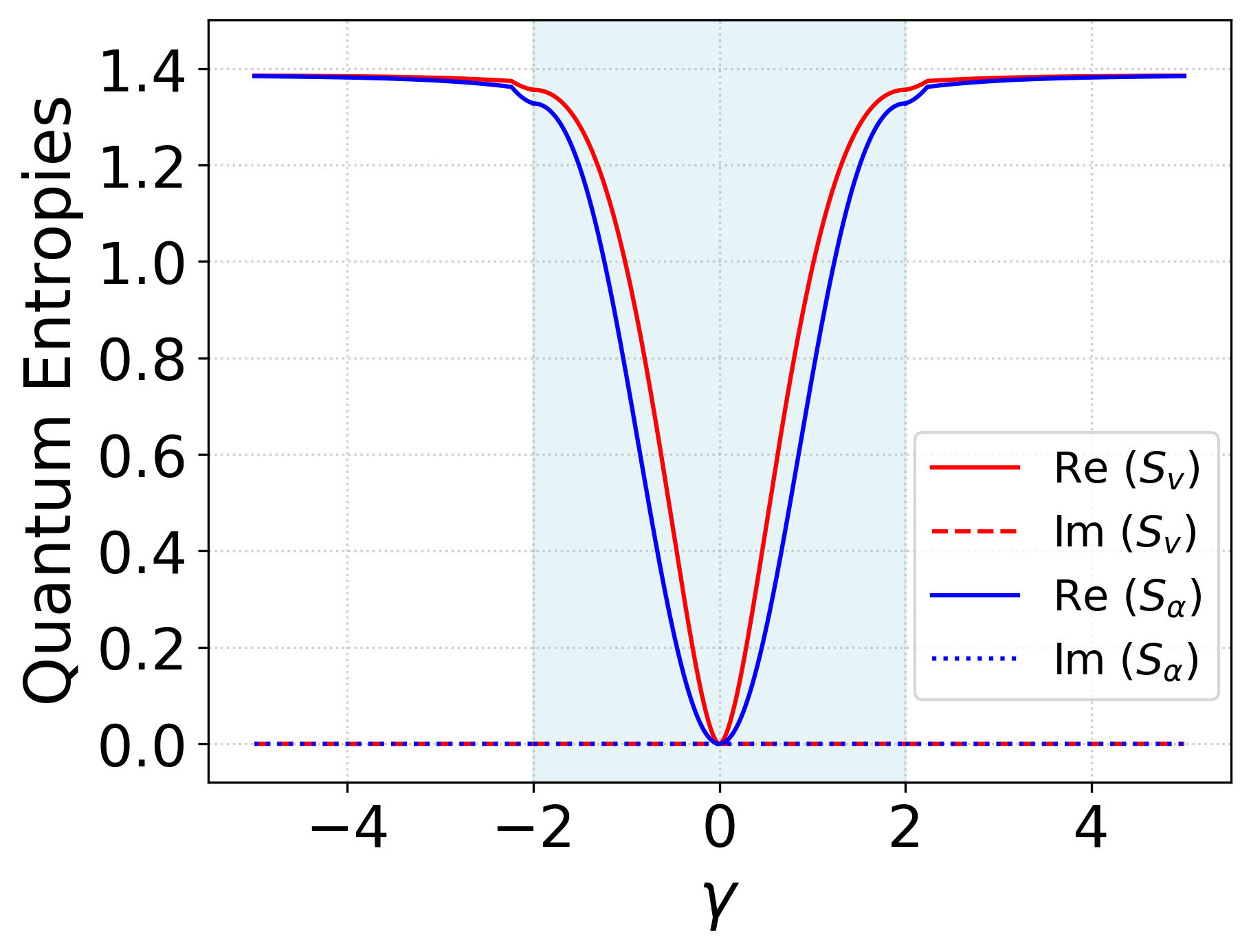
(a)  $n=0$

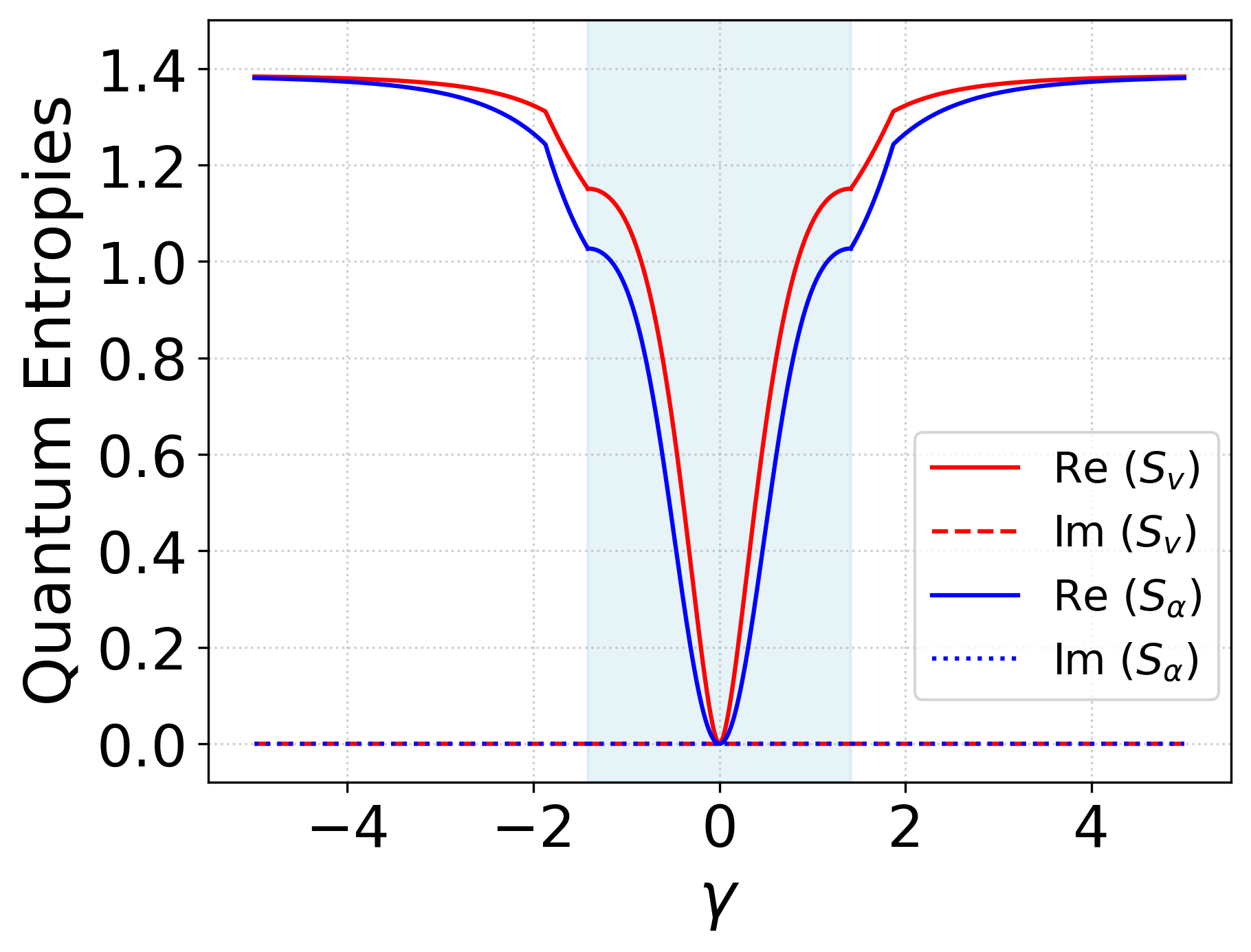
(b)  $n=1$

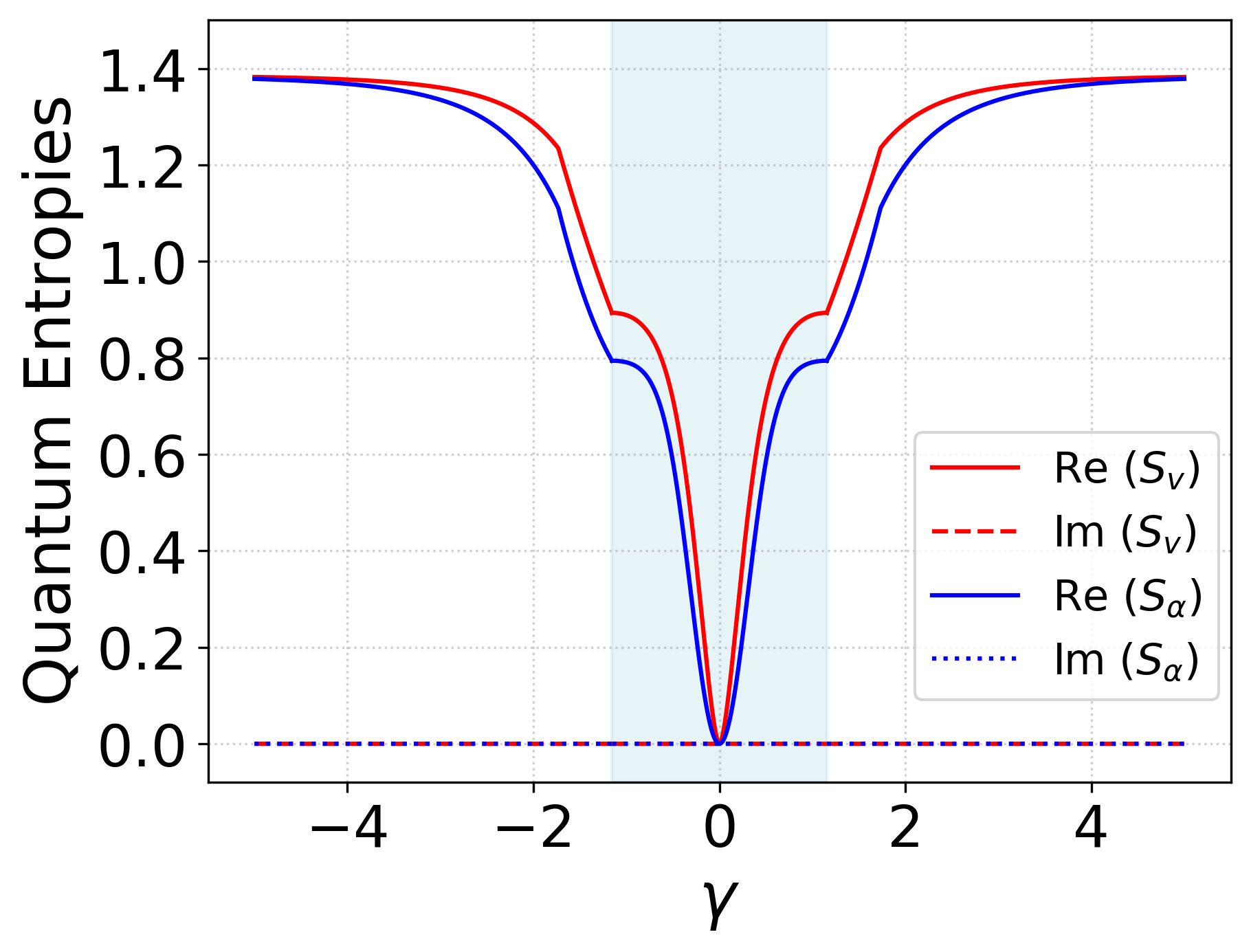
(c)  $n=2$

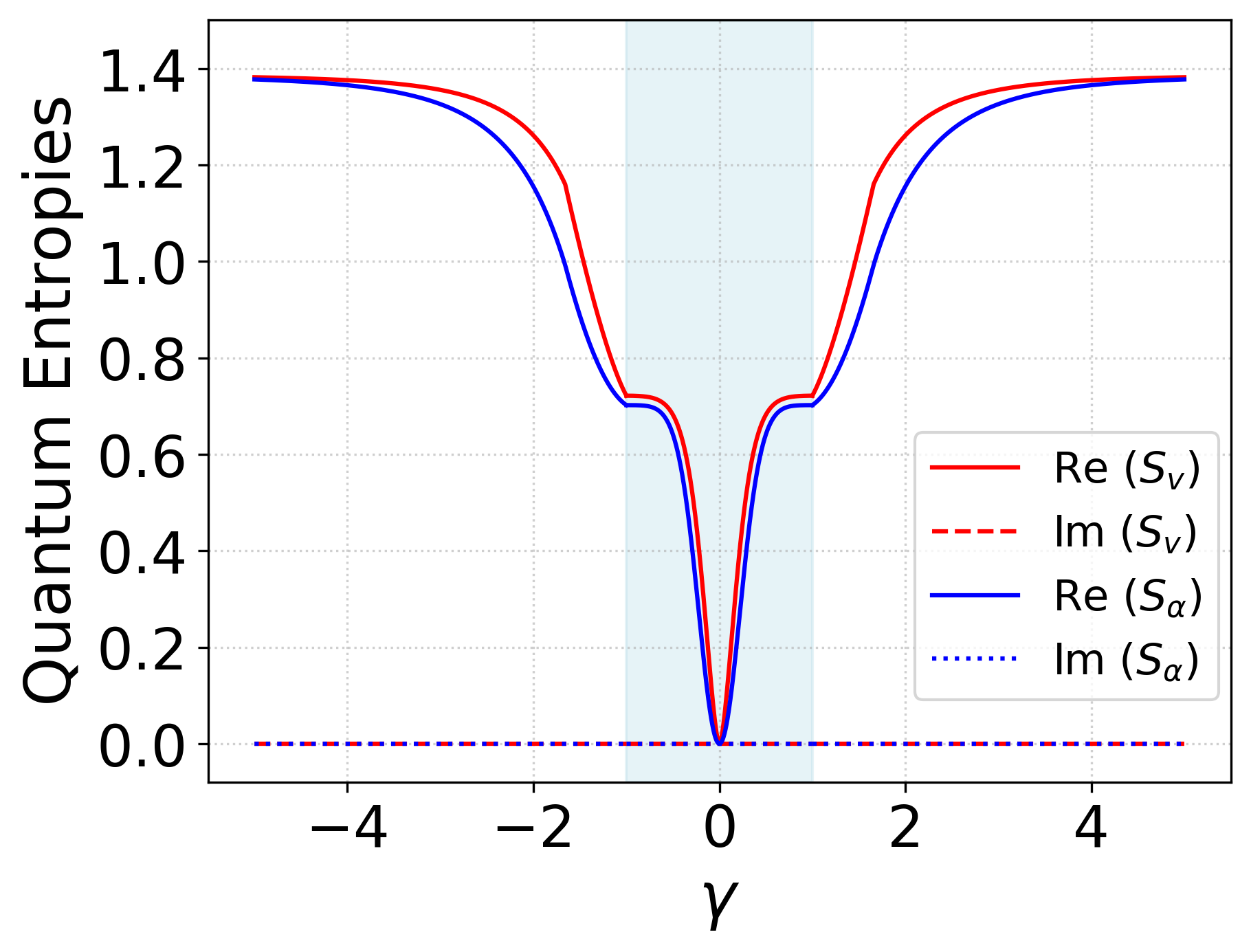
(d)  $n=3$

Figure 3: Variation of the quantum entropies as a function of the real parameter, $\gamma$ for different subspaces for $\alpha=2$. The red and blue lines represent the von Neumann entropy $S_{v}$ and Rényi entropy $S_{\alpha}$ respectively. The unbroken and broken regions are denoted by the shaded (blue) and unshaded regions respectively.

V Quantum Entropies

Concerning the appearance of quantum phase transitions due to the transit from broken to unbroken pseudo-Hermiticity and vice versa, let us investigate how different quantum information-theoretic measures such as the quantum entropies behave at the EP of each invariant subspace. The starting point is the density operator for each invariant subspace, being defined formally as

$$\rho=\sum_{i}p_{i}|\Psi_{i}\rangle\langle\Psi_{i}|$$ (42)

where, $\Psi_{i}$ is the $i^{th}$ eigenstate of a system having probability $p_{i}$ .

For a quantum-mechanical system described by a density matrix $\rho$, the von Neumann entropy $S_{v}$ and Rényi entropy $S_{\alpha}$ of order $\alpha$ ($0<\alpha<\infty$) are defined as follows:

$$S_{v}= -{\rm Tr}(\rho\ln\rho)=-\sum_{i}\beta_{i}\ln\beta_{i}$$ (43)

$$S_{\alpha}= \frac{1}{1-\alpha}\ln[{\rm Tr}(\rho^{\alpha})]=\frac{1}{1-\alpha}\ln\left[\sum_{i}(\beta_{i})^{\alpha}\right]$$

where, $\beta_{i}$, $(i=\rm I,II)$ are the eigenvalues of the density matrix $\rho$

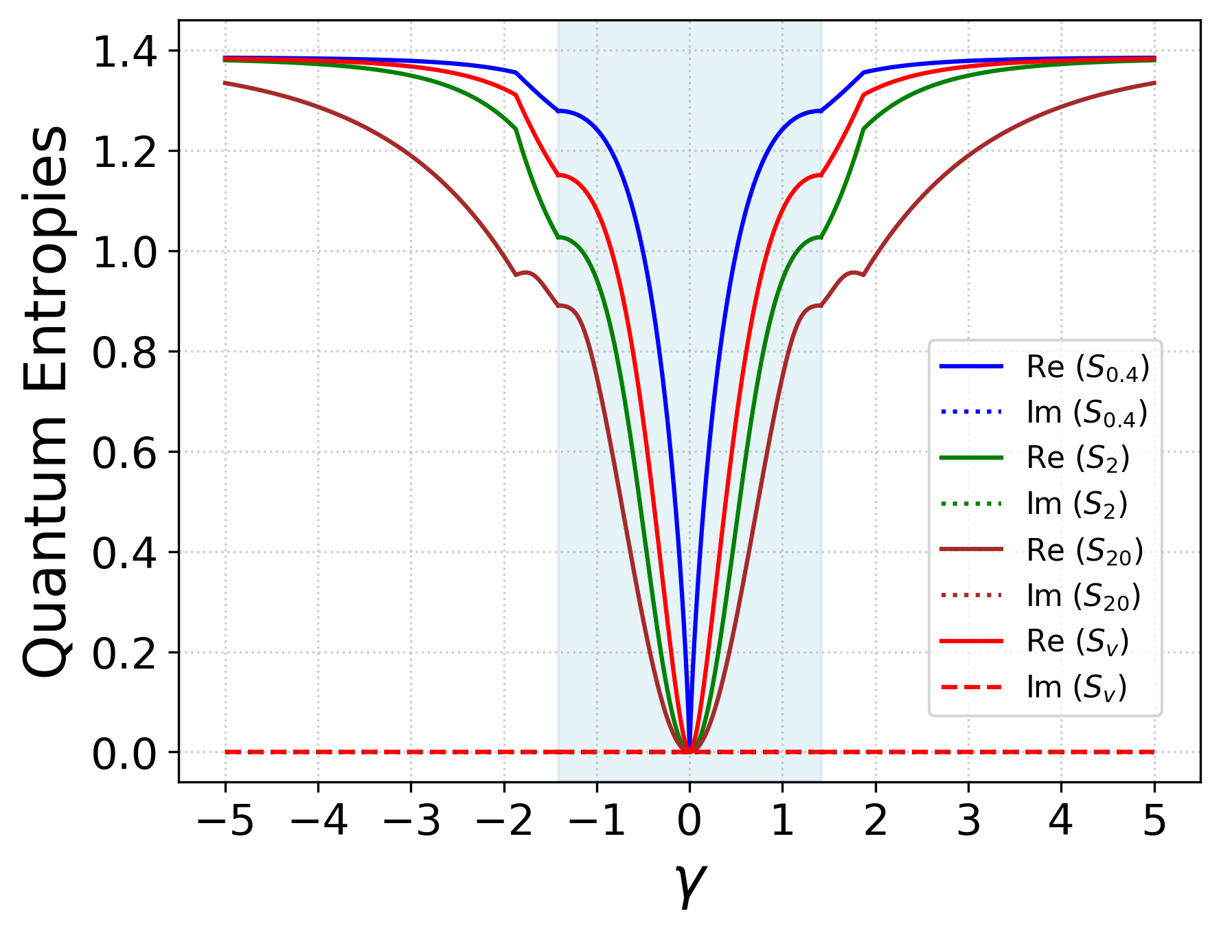
Figure 4: Variation of the quantum entropies as a function of the real parameter, $\gamma$ for different values of alpha for $n=1$. The red line represents the von Neumann entropy, $S_{v}$ and the other plots represent Rényi entropy $S_{\alpha}$ for different values of $\alpha$ as mentioned in the figure. The unbroken and broken regions are denoted by the shaded (blue) and unshaded regions respectively.

V.1 Unbroken region

The density operator, for the $(n+1)^{th}$ subspace in the unbroken region, is obtained using Eqs. (29) and (32) as:

$$\rho_{n+1}=(|\lambda^{i}_{n+1}\rangle\langle\lambda^{i}_{n+1}|)_{G}$$ (44)

where, $|\lambda^{i}_{n+1}\rangle$ $(i=\rm I,II)$ are normalized eigenvectors of the Hamiltonian matrix $(H^{G}_{n+1})$ (given in Eq. (30)). Next, we calculate the reduced density matrix by tracing out the spin degrees of freedom from Eq. (44) as:

$$\rho_{n+1}^{r}= (\langle\frac{1}{2}|\lambda^{i}_{n+1}\rangle\langle\lambda^{i}_{n+1}|\frac{1}{2}\rangle)_{G}+(\langle-\frac{1}{2}|\lambda^{i}_{n+1}\rangle\langle\lambda^{i}_{n+1}|-\frac{1}{2}\rangle)_{G}$$ (45)

$$= \begin{pmatrix}1-\frac{8(2n+1)\delta^{2}}{(2n+1)^{2}\delta^{2}+4(4+\delta^{2})^{2}}&0\\ 0&1+\frac{8(2n+1)\delta^{2}}{(2n+1)^{2}\delta^{2}+4(4+\delta^{2})^{2}}\end{pmatrix}$$

The von Neumann entropy $S_{v}$ and Rényi entropy $S_{\alpha}$ of order $\alpha$ for the $(n+1)^{th}$ subspace in the unbroken region are calculated as (using Eq.  (43)):

$$S_{v_{n+1}} =-\sum_{i}\beta^{i}_{n+1}\ln\beta^{i}_{n+1}$$ (46)

$$S_{\alpha_{n+1}} =\frac{1}{1-\alpha}\ln\left[\sum_{i}(\beta^{i}_{n+1})^{\alpha}\right]$$

where, $\beta^{\rm I,II}_{n+1}$ are the eigenvalues of the reduced density matrix $\rho_{n+1}^{r}$ as given in Eq. (45) for the $(n+1)^{th}$ subspace in the unbroken region.

V.2 Broken region

For the $(n+1)^{th}$ subspace, the density operator, for broken region, is calculated using Eqs. (35) and  (37) as:

$$\tilde{\rho}_{n+1}=(|\tilde{\lambda}^{i}_{n+1}\rangle\langle\tilde{\lambda}^{i}_{n+1}|)_{\tilde{G}}$$ (47)

where, $|\tilde{\lambda}^{i}_{n+1}\rangle$ $(i=\rm I,II)$ are normalized eigenvectors of the Hamiltonian matrix $(\tilde{H}^{G}_{n+1})$ given in Eq. (36). The reduced density matrix for the broken region is then calculated by tracing spin part from Eq. (47) as:

$$\tilde{\rho}_{n+1}^{r}= (\langle\frac{1}{2}|\tilde{\lambda}^{i}_{n+1}\rangle\langle\tilde{\lambda}^{i}_{n+1}|\frac{1}{2}\rangle)_{\tilde{G}}+(\langle-\frac{1}{2}|\tilde{\lambda}^{i}_{n+1}\rangle\langle\tilde{\lambda}^{i}_{n+1}|-\frac{1}{2}\rangle)_{\tilde{G}}$$ (48)

$$= \begin{pmatrix}1-\frac{2n+1}{4+\delta^{2}}&0\\ 0&1+\frac{2n+1}{4+\delta^{2}}\end{pmatrix}$$

The von Neumann entropy $\tilde{S}_{v_{n+1}}$ and Rényi entropy $\tilde{S}_{\alpha_{n+1}}$ of order $\alpha$ are then calculated for the $(n+1)^{th}$ subspace in the broken region by putting the eigenvalues ($\tilde{\beta}^{\rm I,II}_{n+1}$) of $\tilde{\rho}_{n+1}^{r}$ in Eq.  (43).

We have explicitly and analytically calculated $S_{v}$ and $S_{\alpha}$ for both unbroken as well as broken phases of the system for a arbitrary subspace and as a consistency check have verified:

$$\lim_{\alpha\to 1}S_{\alpha}=S_{v}$$ (49)

in both the phases. Expressions for $S_{v}$ and $S_{\alpha}$ are not provided here due to long cumbersome expressions, rather we prefer to analyze these graphically.

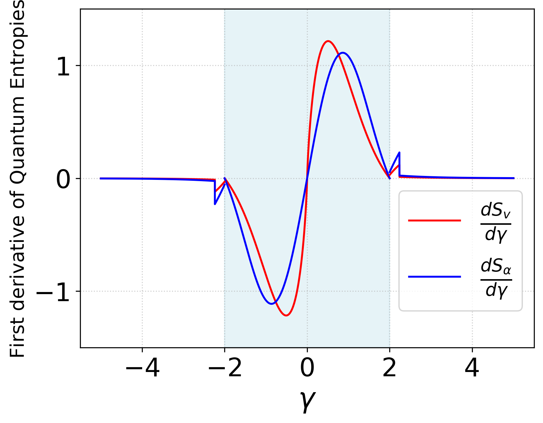
(a)  $n=0$

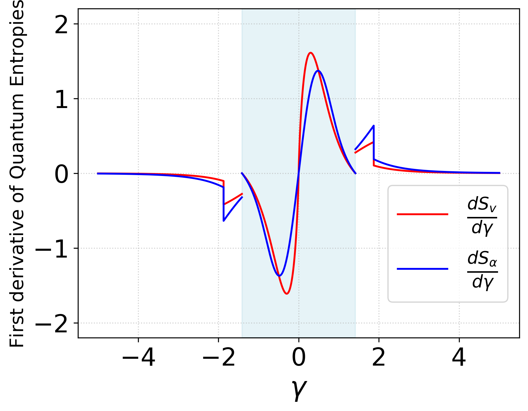
(b)  $n=1$

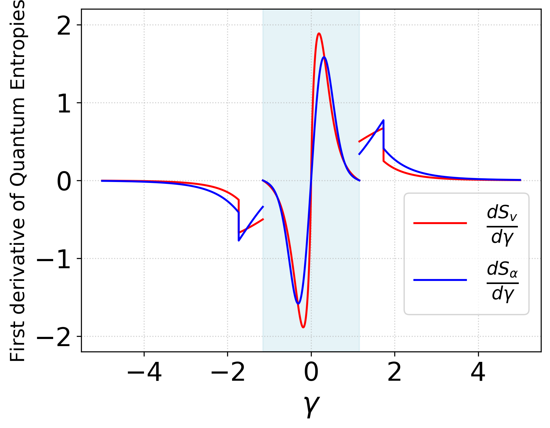
(c)  $n=2$

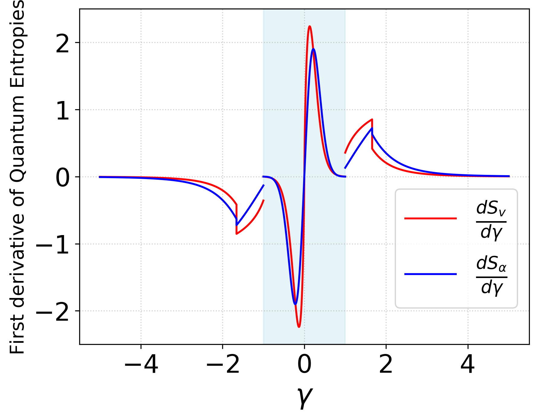
(d)  $n=3$

Figure 5: Variation of the first derivative of quantum entropies as a function of the real parameter, $\gamma$ for different subspaces for $\alpha=2$. The red and blue lines represent the first derivatives of von Neumann entropy $S_{v}$ and Rényi entropy $S_{\alpha}$ respectively. The unbroken and broken regions are denoted by the shaded (blue) and unshaded regions respectively.

In Fig. (3), we have plotted the von Neumann entropy, $S_{v}$ and Rényi entropy $S_{\alpha}$, against the interaction parameter $\gamma$ for different subspaces (n=0,1,2,3). Entropies are always real in both broken and unbroken phases and change abruptly at the EP of that subspace. Entropies saturate at their maximum values for large $\left|\gamma\right|$. The variations of von Neumann entropy and Rényi entropy for different values of $\alpha$ with hermiticity breaking parameter $\gamma$ are depicted in 4. As $\alpha\to 1$, $S_{\alpha}$ gradually converges to $S_{v}$ which is nicely captured in this figure for both the phases. Abrupt changes of these entropies are unaffected in the limit $\alpha\to 1$. First derivatives of the quantum entropies with respect to parameter $\gamma$ for different subspaces are plotted in Fig. 5. It clearly shows the first derivatives for both $S_{v}$ and $S_{\alpha}$ are discontinuous at the EP in all subspaces, indicating a first order quantum phase transition at the EP.

VI Discussion and Results

In this work, we have described some interesting properties of a spin-oscillator system with non-Hermitian coupling. This system can be realised as infinitely-many closed two-dimensional subspaces together with the global ground state. Each two dimensional subspace is associated with an EP, where the eigenvalues along with the corresponding eigenvector coalesce and the system passes from unbroken pseudo-hermitian phase to broken pseudo-hermitian phase or vice versa as illustrated in Figure (1) for different subspaces. Furthur, we compute various information-theoretic measures for this system, namely, the Boltzmann entropy, the von Neumann and R´enyi entropies using the framework of the so-called G-inner product. We have observed that all the quantum entropies are real and positive in both phases and saturate to their maximum values for large $\left|\gamma\right|$. The Boltzmann entropy is real in the unbroken region, but takes up complex values periodically in the broken region due to the complex nature of eigenvalues of the matrix $\tilde{H}^{G}_{n+1}$ given in Eq. (37) in the broken region. It also shows sharp dip and approaches zero at the EP for each subspace as depicted in Figure (2). For the invariant subspaces with higher values of n, the pseudo-Hermitian transition occurs at lower values of $\gamma$, which is also evident from Eq. (23). Unlike the Boltzmann entropy, the quantum entropies are non-zero as we approach the EP. However, the variation of the quantum entropies are abrupt at the EP. The first order derivative of quantum entropies with respect to hermiticity breaking parameter $\gamma$ is discontinuous at the EP leading to the irregular behavior of the entropies at the EP of the theory, as illustrated in Figures (3) and (5). We furthur did a comparative study of the variation of Rényi entropy with respect to $\alpha$. We observe that the slope of the Rényi entropy decreases as value of $\alpha$ increases as shown in Figure (4). To check the robustness of our results, we need to investigate more physical systems.

VII Acknowledgement

G.D. acknowledges UGC-JRF for JRF fellowship. A. G. acknowledges Akash Sinha, Bigchi Bagchi, and Miloslav Znojil for related discussions. B.P.M. acknowledges the incentive research grant for faculty under the IoE Scheme (IoE/Incentive/2021-22/32253) of Banaras Hindu University, Varanasi.

References

- Bender and Boettcher (1998) C. M. Bender and S. Boettcher, Physical review letters 80, 5243 (1998).
- Bender et al. (1999) C. M. Bender, S. Boettcher, and P. N. Meisinger, Journal of Mathematical Physics 40, 2201 (1999).
- Bender et al. (2002) C. M. Bender, D. C. Brody, and H. F. Jones, Physical review letters 89, 270401 (2002).
- Bender (2007) C. M. Bender, Reports on Progress in Physics 70, 947 (2007).
- Mostafazadeh (2010) A. Mostafazadeh, International Journal of Geometric Methods in Modern Physics 7, 1191 (2010).
- Khare and Mandal (2000) A. Khare and B. P. Mandal, Physics Letters A 272, 53 (2000).
- Khare and Mandal (2009) A. Khare and B. P. Mandal, Pramana 73, 387 (2009).
- Mandal et al. (2013) B. P. Mandal, B. K. Mourya, and R. K. Yadav, Physics Letters A 377, 1043 (2013).
- Mandal et al. (2015) B. P. Mandal, B. K. Mourya, K. Ali, and A. Ghatak, Annals of Physics 363, 185 (2015).
- Raval and Mandal (2019) H. Raval and B. P. Mandal, Nuclear Physics B 946, 114699 (2019).
- Mandal (2021) B. P. Mandal, in Journal of Physics: Conference Series (IOP Publishing, 2021), vol. 2038, p. 012017.
- Modak and Mandal (2021) R. Modak and B. P. Mandal, Physical Review A 103, 062416 (2021).
- Pal et al. (2025) T. Pal, R. Modak, and B. P. Mandal, Physical Review E 111, 014421 (2025).
- Ghatak et al. (2013) A. Ghatak, R. D. R. Mandal, and B. P. Mandal, Annals of Physics 336, 540 (2013).
- Hasan and Mandal (2018) M. Hasan and B. P. Mandal, Annals of Physics 396, 371 (2018).
- Hasan et al. (2020) M. Hasan, V. N. Singh, and B. P. Mandal, The European Physical Journal Plus 135, 640 (2020).
- Basu-Mallick and Mandal (2001) B. Basu-Mallick and B. P. Mandal, Physics Letters A 284, 231 (2001).
- Basu-Mallick et al. (2004) B. Basu-Mallick, T. Bhattacharyya, A. Kundu, and B. P. Mandal, Czechoslovak journal of physics 54, 5 (2004).
- Bender et al. (2013) C. M. Bender, B. K. Berntson, D. Parker, and E. Samuel, American Journal of Physics 81, 173 (2013).
- Mandal and Ghatak (2012) B. P. Mandal and A. Ghatak, Journal of Physics A: Mathematical and Theoretical 45, 444022 (2012).
- Ghatak et al. (2015) A. Ghatak, M. Hasan, and B. P. Mandal, Physics Letters A 379, 1326 (2015).
- Hajong et al. (2024) G. Hajong, R. Modak, and B. P. Mandal, Physical Review A 109, 022227 (2024).
- Dwivedi and Mandal (2021) A. Dwivedi and B. P. Mandal, Annals of Physics 425, 168382 (2021).
- Hasan and Mandal (2020a) M. Hasan and B. P. Mandal, The European Physical Journal Plus 135, 1 (2020a).
- Banerjee et al. (2024) S. Banerjee, R. K. Yadav, A. Khare, and B. P. Mandal, Journal of Mathematical Physics 65 (2024).
- Bhowmick et al. (2025) B. Bhowmick, R. M. Shinde, and B. P. Mandal, International Journal of Theoretical Physics 64, 34 (2025).
- Hasan and Mandal (2020b) M. Hasan and B. P. Mandal, Journal of Mathematical Physics 61 (2020b).
- Hajong et al. (2025) G. Hajong, R. Modak, and B. P. Mandal, arXiv preprint arXiv:2504.20167 (2025).
- Brihaye et al. (2007) Y. Brihaye, A. Nininahazwe, and B. P. Mandal, Journal of Physics A: Mathematical and Theoretical 40, 13063 (2007).
- Mandal and Gupta (2010) B. P. Mandal and S. Gupta, Modern Physics Letters A 25, 1723 (2010).
- Kumari et al. (2016) N. Kumari, R. K. Yadav, A. Khare, B. Bagchi, and B. P. Mandal, Annals of Physics 373, 163 (2016).
- Mostafazadeh (2002a) A. Mostafazadeh, Journal of Mathematical Physics 43, 3944 (2002a).
- Mostafazadeh (2002b) A. Mostafazadeh, Journal of Mathematical Physics 43, 205 (2002b).
- Kretschmer and Szymanowski (2004) . R. Kretschmer and L. Szymanowski, Physics Letters A 325, 112 (2004).
- Ghatak and Mandal (2013) A. Ghatak and B. P. Mandal, Communications in Theoretical Physics 59, 533 (2013).
- Goldzak et al. (2018) T. Goldzak, A. A. Mailybaev, and N. Moiseyev, Physical review letters 120, 013901 (2018).
- Sinha et al. (2024) A. Sinha, A. Ghosh, and B. Bagchi, Physica Scripta 99, 105534 (2024).
- Bagarello et al. (2025) F. Bagarello, F. Gargano, and L. Saluto, Journal of Mathematical Physics 66 (2025).
- Fring and Frith (2019) A. Fring and T. Frith, Physical Review A 100, 010102 (2019).
- Wehrl (1978) A. Wehrl, Reviews of Modern Physics 50, 221 (1978).
- Casini and Huerta (2009) H. Casini and M. Huerta, Journal of Physics A: Mathematical and Theoretical 42, 504007 (2009).
- Rényi (1961) A. Rényi, in Proceedings of the fourth Berkeley symposium on mathematical statistics and probability, volume 1: contributions to the theory of statistics (University of California Press, 1961), vol. 4, pp. 547–562.
- Mandal (2005) B. P. Mandal, Modern Physics Letters A 20, 655 (2005).
- Brody (2013) D. C. Brody, Journal of Physics A: Mathematical and Theoretical 47, 035305 (2013).
- Shukla et al. (2023) N. Shukla, R. Modak, and B. P. Mandal, Physical Review A 107, 042201 (2023).
- Ju et al. (2019) C.-Y. Ju, A. Miranowicz, G.-Y. Chen, and F. Nori, Physical Review A 100, 062118 (2019).
- Tzeng et al. (2021) Y.-C. Tzeng, C.-Y. Ju, G.-Y. Chen, and W.-M. Huang, Physical Review Research 3, 013015 (2021).