Type II Seesaw Leptogenesis in a Majoron background

Abstract

We discuss spontaneous Leptogenesis in the Type II Seesaw model of neutrino masses featuring an electroweak triplet scalar $T$ in a coherent pseudo Nambu-Goldstone boson (pNGB) background. In the wash-in scenario the inverse decays of Higgs bosons to $T$ generate a chemical potential for the triplet that is then transmitted to the lepton sector via the leptonic decays of $T$. Our mechanism works with a single triplet that can be as light as 1 TeV, and has a vacuum expectation value $v_{T}$ in the window $\mathcal{O}($1\text{\,}\mathrm{keV}$)<v_{T}<\mathcal{O}($1\text{\,}\mathrm{MeV}$)$. This range of $v_{T}$ can lead to appreciable decays of the triplet’s doubly charged component into both same sign di-leptons and same sign pairs of $W$-bosons, which could potentially allow for an experimental distinction from a recently proposed inflationary Type II Seesaw Affleck-Dine scenario preferring the leptonic mode. In the singlet-doublet-triplet Majoron UV-completion of the Type II Seesaw model, the required pNGB is automatically included in the form of the Majoron that originates from the phase of the lepton number breaking singlet scalar. The coherent motion of the Majoron can furthermore explain the dark matter relic abundance via the kinetic misalignment mechanism. Cogenesis of dark matter and the baryon asymmetry can work for a lepton number breaking scale of $\mathcal{O}(${10}^{5}\text{\,}\mathrm{GeV}$)<v_{\sigma}<\mathcal{O}(${10}^{8}\text{\,}\mathrm{GeV}$)$ and a Majoron mass of $\mathcal{O}($1\text{\,}\mathrm{eV}$)>m_{j}>\mathcal{O}($1\text{\,}\mathrm{\SIUnitSymbolMicro eV}$)$.

1 Introduction

1.1 Overview

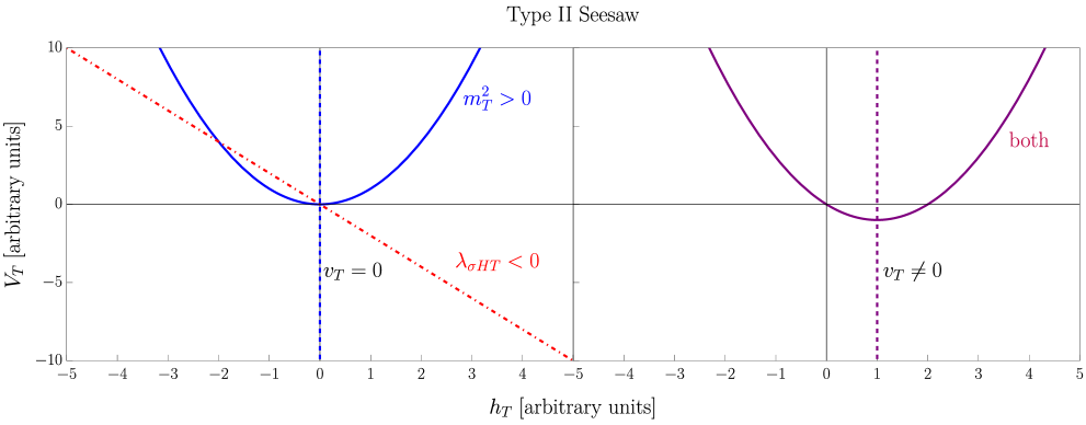
Figure 1: Basic overview for how a parametrically small triplet vev $v_{T}$ can be generated in the Type II Seesaw mechanism. The triplet has a positive mass squared (blue, left) that by itself would lead to a trivial minimum $v_{T}=0$. After lepton number and the SM gauge symmetry are spontaneously broken by the vevs $v_{\sigma}$, $v_{H}$ of $\sigma$ and $H$ respectively, there exists a linear term in the triplet potential proportional to $\kappa=\lambda_{\sigma HT}v_{\sigma}/\sqrt{2}$ (red, left) from Eq. (2.3), which tilts the potential to generate a small $v_{T}\neq 0$ (purple, right). Here $h_{T}$ denotes the field value of the electrically neutral, $CP$ even component of $T$ and $V_{T}$ is the potential energy. The plot is not up to scale and all parameters were chosen for illustration only.

Non-vanishing neutrino masses have been robustly established from numerous observations of neutrino flavor oscillations at different length scales (see Refs.[1, 2] for an overview), and a precise measurement of the $\beta$-decay spectrum by the KATRIN collaboration [3]. Consequently the massive nature of neutrinos provides unambiguous evidence for physics beyond the Standard Model (SM). The Type II Seesaw mechanism [4, 5, 6, 7, 8] stands out among the three known tree level UV completions of the Weinberg operator [9] for parametrically small Majorana neutrino masses, because it is the only one that relies on a scalar mediator in the form of electroweak triplet $T$ carrying hypercharge. Another distinction is given by the fact that it is the only tree level scheme for Majorana neutrino masses that predicts the existence of electrically double charged particles, which might be accessible at collider experiments due to their couplings to electroweak gauge bosons. Similar to the right handed gauge singlet neutrino of the Type I Seesaw [13, 14, 15, 16] the scalar triplet can be accommodated in the grand unified theory $\text{SO}(10)$, where it usually appears together with the Type I Seesaw.

At its core the Type II Seesaw mechanism can also be understood as sourcing a parametrically small vacuum expectation value (vev) $v_{T}$ for the neutral component of the triplet, that can be closer to the observed scale of neutrino masse than the vev of the SM Higgs. This occurs because the positive quadratic potential for the triplet $m_{T}^{2}|T|^{2}$ is biased in one direction by the impact of the term $\kappa H^{t}\varepsilon TH\;(\varepsilon=i\sigma_{2})$ after the neutral component of the Higgs doublet condenses with a vev $v_{H}$. Here $\kappa$ is a coupling of mass dimension one, that is a priori unrelated to any other energy scale and it can be understood as a spurion of the global lepton number symmetry $\text{U}(1)_{L}$ with charge minus two. A schematic illustration of the origin of this minimum with $v_{T}\neq 0$ can be observed in Fig. 1.

Where the previously described model breaks lepton number explicitly and induces a vev for $T$, one could also try to use the triplet to spontaneously break $\text{U}(1)_{L}$ with e.g. an eV-scale vev. Such a model gives rise to a Nambu-Goldstone boson (NGB) known as the triplet Majoron [17]. However since the massless Majoron arises from a hypercharged weak multiplet, it would be produced in decays of the $Z$ boson. In fact this decay mode would contribute more than one additional generations of neutrinos to the $Z$-width, which is robustly ruled out by data from LEP 1 [18]. This serious caveat is absent in models that utilize a scalar gauge singlet to spontaneously break lepton number, and their NGBs are usually referred to as singlet Majorons [19, 20].

Nevertheless one can salvage the triplet Majoron via a synthesis with the Type II Seesaw: In the singlet-doublet-triplet model [29, 30, 31] the dimensionful spurion $\kappa$ is UV completed via the vev $v_{\sigma}$ of a singlet scalar $\sigma$ that predominantly houses the Majoron and one obtains $\kappa=\lambda_{\sigma HT}v_{\sigma}/\sqrt{2}$ in terms of the dimensionless scalar coupling $\lambda_{\sigma HT}$. The advantage of having a Majoron in the spectrum is that it can be a good dark matter (DM) candidate (see Refs. [32, 33, 34, 35] for an overview), if further explicit breaking of $\text{U}(1)_{L}$ renders it to be a massive pseudo Nambu-Goldstone boson (pNGB). Previous analyses of dark matter in the singlet-doublet-triplet Majoron scenario can be found in Refs. [36, 37].

It has been known for a long time that the neutrino sector can not just help with the problem of dark matter, but it can also address the origin of the observed asymmetry between matter and anti-matter of $\Delta_{B}=8.76\times 10^{-11}$ [38, 39] via the mechanism known as Leptogenesis [40] from the out-of-equilibrium decays of the heavy Seesaw mediators. Type II Seesaw Leptogenesis was first studied in Refs. [41, 42, 43, 44], and whereas neutrino masses only need a single triplet, the $CP$-violation in the out-of-equilibrium decay scenario requires at least two such generations. For a hierarchical triplet spectrum one needs [44]

$$m_{T}>\mathcal{O}(${10}^{10}\text{\,}\mathrm{GeV}$),$$ (1.1)

to explain the observed baryon asymmetry, which is about one order of magnitude stronger than the limit on the right handed neutrino masses in Type I Seesaw Leptogenesis [45]. This estimate illustrates, why it is almost hopeless to test the required $m_{T}$ with laboratory experiments. A resonant enhancement of the self-energy graphs on the other hand could bring the needed triplet mass down to the TeV-scale at the cost of having at least two almost degenerate triplets [46, 47].

An elegant resolution of the previously motivated problems can be found in non-thermal Leptogenesis scenarios of the Affleck-Dine archetype [48, 49, 50]. Here the required $CP$ violation comes from the coherent motion of a scalar field in the complex plane, and a single triplet suffices. The coherent rotation of the condensate is possible due to a phase-dependent scalar interactionl, that explicitly violates baryon- or lepton-number. At the end of the scalar field’s evolution its baryonic or leptonic charge is dumped into the plasma via decays, which lends itself naturally to post-inflationary reheating, especially in models that identify the Affleck-Dine field with the inflaton. The idea of inflation from a non-minimal coupling to gravity was merged with the Type II Seesaw and Affleck-Dine Leptogenesis in Refs. [51, 52], and this set-up was further discussed in Refs. [53, 54]. Such an approach can also work with TeV-scale triplets, and avoiding the washout of the leptonic asymmetry into the Higgs sector limits the triplet vev to be [51, 52]

$$v_{T}<$8.5\text{\,}\mathrm{keV}$\sqrt{\frac{$1\text{\,}\mathrm{TeV}$}{m_{T}}}.$$ (1.2)

1.2 This work

The second staple of non-thermal Baryogenesis scenarios from the coherent motion of a scalar field is known as Spontaneous Baryogenesis [55, 56] (see Ref. [57] for a review). In its minimal form this scenario involves only a single $CP$ odd scalar, that eventually begins to oscillate around the minimum of its potential. The key idea is that the pseudoscalar’s field velocity $\dot{\theta}$ evolves as an adiabatic background field, that spontaneously violates $CPT$ and can thus allow for asymmetry production in thermal equilibrium. The trade-off is that one needs to supply an additional baryon- or lepton-number violating interaction, that is active in the plasma, and decouples eventually. Here interactions that would usually “wash-out” the baryon- or lepton number asymmetry in the out-of-equilibrium decay scenario, instead “wash-in” the asymmetry [58]. A natural realization of this mechanism is found in heavy Majoron models [59, 60] (see also Ref. [61] for a recent implementation in the singlet-doublet-triplet model). The needed Majorons typically overclose the universe, or are not long-lived enough to be the dark matter [62].

In recent years this idea has received renewed attention, because the authors of Refs. [63, 64] realized that the pNGB velocity $\dot{\theta}$ , that drives spontaneous Baryogenesis, can be induced via the Affleck-Dine mechanism. The prerequisite explicit breaking of e.g. baryon- or lepton-number then automatically generates a mass for the NGB in question [65, 66] and the pNGBs can be much lighter than in the original spontanoues Baryogenesis scenario. It was shown in Ref. [63] that the pNGB rotation experiences only a negligible back-reaction from driving Baryogenesis, which is why it can survive until late times, and source the dark matter relic abundance via the kinetic misalignment mechanism [67, 68, 69] (see also [70]). This idea stimulated a lot of studies [71, 72, 73, 74, 75, 76, 77, 78, 79, 80, 81, 82], and was applied to both theories of Dirac neutrino masses in Ref. [83, 65], as well as to Majorana neutrino masses in Refs. [84, 62, 66].

An investigation of these dynamics in a Type I Seesaw context [62] revealed that “wash-in” Leptogenesis can proceed via the inverse decays $LH\rightarrow N$, where $N$ is a right handed neutrino. This approach has an additional benefit, that has not received a lot of attention so far: It can also significantly lower the right handed neutrino mass scale down to values above $2\text{\,}\mathrm{GeV}$, where the lower limit comes from the cosmological self-consistency of the analysis. In a similar vein Ref. [79] obtained an upper limit of $10\text{\,}\mathrm{GeV}$ in the context of asymmetry production from scattering in a supersymmetric QCD axion model. Apart from the attractive features of a built-in dark matter candidate and production mechanism, this makes Leptogenesis in a Majoron background a serious candidate for low-scale Leptogenesis, all without quasi-degenerate Seesaw mediators, or even multiple genrations of mediators. In particular we expect the discussion of Ref. [62] to also apply to the hypercharge-less triplet fermions of the Type III Seesaw [85], where the lowest triplet mass is already constrained by collider searches at the LHC to be at or above the TeV-scale [86, 87].

The present work follows this path and adapts it to the peculiarities of the Type II Seesaw. In particular our scenario works with a single generation of scalar triplets, whose mass is only limited by bounds from laboratory experiments and could well be close to the TeV-scale. Here the inverse decay of two Higgses $HH\rightarrow T$ first generates a chemical potential for $T$ proportional to $\dot{\theta}$ that is then transmitted to the lepton sector via the decays $T\rightarrow L^{\dagger}L^{\dagger}$. We do not consider a rotation of the triplet, but rather employ it as an intermediate reservoir for the asymmetry, which works, because it is not self-conjugate. In the “strong wash-in” regime, where both of the aforementioned processes are fast on cosmological time scales, we predict that the triplet vev lies in the following window

$$$8.5\text{\,}\mathrm{keV}$\sqrt{\frac{$1\text{\,}\mathrm{TeV}$}{m_{T}}}<v_{T}<$277\text{\,}\mathrm{keV}$\sqrt{\frac{$1\text{\,}\mathrm{TeV}$}{m_{T}}}\sqrt{\frac{\overline{m}_{\nu}^{2}}{$2.65\text{\times}{10}^{-3}\text{\,}{\mathrm{eV}}^{2}$}}.$$ (1.3)

However out set-up can also work outside of this window in the “weak wash-in” regime, so that a larger range of

$$\mathcal{O}($1\text{\,}\mathrm{keV}$)<v_{T}<\mathcal{O}($1\text{\,}\mathrm{MeV}$)$$ (1.4)

is viable. In principle these ranges for $v_{T}$ allow our model to be experimentally distinguished from the inflationary Affleck-Dine scenario of Refs. [51, 52, 53, 54], that predicts the different range of $v_{T}$ shown in Eq. (1.2). For completeness we also discuss the high-scale scenario with a super-heavy triplet $m_{T}\gtrsim\mathcal{O}(${10}^{14}\text{\,}\mathrm{GeV}$)$, that is too heavy to be present in the plasma, and corresponds to the well studied regime of spontaneous Leptogenesis from the Weinberg-operator. If the radial mode of $\sigma$ has a large field value, this high-scale regime only works for a narrow range of parameters.

This manuscript is structured in the following way: We begin with a review over the Type II Seesaw model and its associated phenomenology in section 2. Then we provide an overview over the phenomenological aspects of the singlet-doublet-triplet Majoron in section 3, where special emphasis is put on a review of the known mechanisms for generating a time dependent Majoron condensate, including the Affleck-Dine scheme in subsection 3.2.1 and a host of alternatives in subsection 3.2.2. Majoron dark matter from the kinetic misalignment mechanism and its detection prospects are discussed in section 4. We encourage the avid reader, that is already familiar with these subjects, to directly skip ahead to sections 5-6, where the key features of our Leptogenesis scenario are discussed in detail. The combined parameter space from all these ingredients is displayed in Figs. 3, 6 and 7. Section 6 discusses the high scale scenario, where the triplet is too heavy to be in the thermal bath, and contains our arguments, for why we do not focus on this specific region of parameter space. The details of our predictions will be elucidated in section 7, before we provide our conclusions in section 8. Appendix A explicitly demonstrates that the effective chemical potential prescription in a Majoron background also holds for bosons coupled to the Majoron. Appendix B explains why we do not consider a rotation of the triplet scalar itself.

2 Type II Seesaw

In this section we introduce the Type II Seesaw model [4, 5, 6, 7, 8] in the “singlet-doublet-triplet” formulation [29, 30, 31], and review its salient phenomenological aspects.

2.1 The Model

Figure 2: Diagrammatic representation of the dimension six operator for the Type II Seesaw with spontaneously broken lepton number giving rise to Majorana masses for the active neutrinos. The arrows of the fermion line correspond to their chirality following the two-component spinor notation of Ref. [88].

We introduce an electroweak scalar triplet $T$ with hypercharge $Q_{Y}[T]=1$ and lepton number $Q_{L}[T]=-2$ that can be decomposed as

$$T=\begin{pmatrix}\frac{T^{+}}{\sqrt{2}}&T^{++}\\ T^{0}&-\frac{T^{+}}{\sqrt{2}}\end{pmatrix},$$ (2.1)

together with an SM singlet scalar $\sigma$ with $Q_{L}[\sigma]=2$

$$\sigma=\frac{h_{\sigma}+v_{\sigma}}{\sqrt{2}}e^{i\frac{j}{v_{L}}},$$ (2.2)

where $v_{\sigma}$ is the scale of lepton number breaking and $j$ the Majoron. The relevant interactions with the lepton doublet $L$ and the Higgs doublet $H$ read

$$-\mathcal{L} =y_{L}L^{t}\varepsilon TL+\text{h.c.},$$ (2.3)

$$V(\sigma,H,T) \subset m_{T}^{2}\text{Tr}\left(T^{\dagger}T\right)+\lambda_{\sigma HT}\sigma H^{\dagger}\varepsilon TH^{*}+\text{h.c.},$$ (2.4)

where $\varepsilon=i\sigma_{2}$ in terms of the second Pauli matrix is needed to symmetrize the $\text{SU}(2)$ contractions. Throughout this work we use the two-component spinor notation of Ref. [88]. The full scalar potential can be found in e.g. Ref. [37] and the coupling $\lambda_{\sigma HT}$ can be made real by a field redefinition of either $\sigma$ or $T$. Consequently a complex vev $v_{T}$ can only arise from spontaneous $CP$ violation, which requires at least two triplets [89]. The necessary and sufficient conditions for vacuum stability were compiled in Ref. [90].

We take $m_{T}^{2}>0$ and assume the following potential for the spontaneous breaking of lepton number

$$V_{\sigma}=\lambda_{\sigma}(v_{\sigma}^{2}-|\sigma|^{2})^{2}.$$ (2.5)

At low energies one can integrate out the triplet to obtain the following dimension six operator depicted in Fig. 2

$$y_{L}\lambda_{\sigma HT}\frac{v_{H}^{2}}{m_{T}^{2}}\;\sigma^{*}(LH)^{2},$$ (2.6)

which reduces to the well known dimension five Weinberg-operator $(LH)^{2}$ [9] once the lepton number breaking scalar $\sigma$ condenses. Non-zero values for the vev $v_{H}$ of the neutral component of $H$ and $v_{\sigma}$ induce a vev for the neutral component of the triplet (see Fig. 1 for an illustration)

$$v_{T}=\lambda_{\sigma HT}\frac{v_{\sigma}v_{H}^{2}}{m_{T}^{2}},$$ (2.7)

and the neutrino mass is found to be

$$m_{\nu}=y_{L}\frac{v_{T}}{\sqrt{2}}.$$ (2.8)

Taking $m_{T}^{2}\gg\lambda_{\sigma HT}v_{\sigma}v_{H}$ ensures that $v_{T}\ll v_{H}$. In this work we will focus on a TeV-scale triplet with $\mathcal{O}($1\text{\,}\mathrm{keV}$)<v_{T}<\mathcal{O}($1\text{\,}\mathrm{MeV}$)$ and $v_{\sigma}>\mathcal{O}(${10}^{5}\text{\,}\mathrm{GeV}$)$, for which the neutrino mass scale is realized via small $\lambda_{\sigma HT}$ and $y_{L}$. The role of the spontaneously broken $\text{U}(1)_{L}$ symmetry is to ultra-violet (UV) complete the commonly assumed explicit lepton number breaking term $\kappa H^{t}\varepsilon TH$ via the identification $\kappa=\lambda_{\sigma HT}v_{\sigma}/\sqrt{2}$.

2.2 Phenomenology

process	type	$v_{T}>$	experiment	reference
$\mu\rightarrow e\gamma$	limit	$$0.95\text{\,}\mathrm{eV}$\left(\frac{$1\text{\,}\mathrm{TeV}$}{m_{T}}\right)$	MEG	[91]
	projection	$$1.85\text{\,}\mathrm{eV}$\left(\frac{$1\text{\,}\mathrm{TeV}$}{m_{T}}\right)$	MEGII	[92]
$\mu\rightarrow 3e$	limit	$\left(\frac{$1\text{\,}\mathrm{TeV}$}{m_{T}}\right)\begin{cases}$0.45\text{\,}\mathrm{eV}$\;\text{(NO)}\\ $0.98\text{\,}\mathrm{eV}$\;\text{(IO)}\end{cases}$	SINDRUM	[93]
	projection	$\left(\frac{$1\text{\,}\mathrm{TeV}$}{m_{T}}\right)\begin{cases}$4.54\text{\,}\mathrm{eV}$\;\text{(NO)}\\ $9.83\text{\,}\mathrm{eV}$\;\text{(IO)}\end{cases}$	Mu3e	[94]
$\mu-e\;\text{conversion}$	limit (Ti)	$$9.10\text{\,}\mathrm{eV}$\left(\frac{$1\text{\,}\mathrm{TeV}$}{m_{T}}\right)\sqrt{\frac{4v_{T}^{2}|C_{\mu e}^{(II)}|}{$1\text{\,}\mathrm{eV}$}}$	SINDRUMII	[95]
	limit (Al)	$$71.86\text{\,}\mathrm{eV}$\left(\frac{$1\text{\,}\mathrm{TeV}$}{m_{T}}\right)\sqrt{\frac{4v_{T}^{2}|C_{\mu e}^{(II)}|}{$1\text{\,}\mathrm{eV}$}}$	Mu2e	[96]

Table 1: Bounds on the vev $v_{T}$ from lepton flavor violation. The limits were adapted from Refs. [97, 98].

Most of the Type II Seesaw phenomenology is controlled by the two parameters $v_{T}$ and $m_{T}$, together with the sum of squared neutrino masses $\sum_{i}m_{\nu_{i}}^{2}$. For the numerical evaluation of this quantity we take the mass splittings from the global fit in Ref. [2], and impose the constraint on the sum of neutrino masses $\sum_{i}m_{\nu_{i}}<$0.12\text{\,}\mathrm{eV}$$ [38] from Planck temperature and polarization data together with information from gravitational lensing and BAO

(NO)$$2.65\text{\times}{10}^{-3}\text{\,}{\mathrm{eV}}^{2} <\overline{m}_{\nu}^{2}\equiv\sum_{i}m_{\nu_{i}}^{2}<$5.34\text{\times}{10}^{-3}\text{\,}{\mathrm{eV}}^{2}$,$$ (2.9)

(IO)$$4.92\text{\times}{10}^{-3}\text{\,}{\mathrm{eV}}^{2} <\overline{m}_{\nu}^{2}\equiv\sum_{i}m_{\nu_{i}}^{2}<$5.68\text{\times}{10}^{-3}\text{\,}{\mathrm{eV}}^{2}$,$$ (2.10)

where NO (IO) denotes normal (inverted) mass ordering. The lower value refers to the case of a massless lightest neutrino and the upper value comes from saturating the cosmological limit. Throughout this work we limit ourselves to the NO mass hierarchy and fix

$$\overline{m_{\nu}}^{2}=$2.65\text{\times}{10}^{-3}\text{\,}{\mathrm{eV}}^{2}$.$$ (2.11)

The mass eigenstates of the triplet are given by the $CP$ even (odd) $h_{T}\;(a_{T})$, the singly charged $h^{\pm}$ and the doubly charged $h^{\pm\pm}$ that are (mostly) aligned with the gauge eigenstates $T^{0},T^{\pm}$ and $T^{\pm\pm}$. Their mass spectrum reads in the limit $v_{H}\gg v_{T}$

$$m_{h_{T}}^{2}\simeq m_{a_{T}}^{2}\simeq m_{h^{\pm}}^{2}+\frac{\lambda_{HT2}}{4}v_{H}^{2}\simeq m_{h^{\pm\pm}}^{2}+\frac{\lambda_{HT2}}{2}v_{H}^{2}\simeq m_{T}^{2},$$ (2.12)

where $\lambda_{HT2}$ is the coefficient of the term $\text{Tr}\left(H^{\dagger}T^{\dagger}TH\right)$, and a full overview over the masses and mixing can be found in Ref. [37]. Electroweak precision data further constrains the mass splitting between the doubly and singly-charged scalar [108, 109, 110, 111]

$$|m_{h^{\pm\pm}}-m_{h^{\pm}}|<$40\text{\,}\mathrm{GeV}$.$$ (2.13)

In this work we will consider either $m_{T}^{2}\gg v_{H}^{2}$ or $\lambda_{HT2}\ll 1$, which limits the discussion to a degenerate mass spectrum of common mass $m_{T}$. We denote the mass eigenstate that predominantly arises from the radial mode of $\sigma$ as $h_{\sigma}$ and its mass reads

$$m_{S}^{2}\simeq 2\lambda_{\sigma}v_{\sigma}^{2}.$$ (2.14)

We introduce the $CP$ even boson, that predominantly arises from the neutral component of $H$, as $h_{H}$, and identify it with the $125\text{\,}\mathrm{GeV}$ resonance observed at the LHC.

The doubly charged scalar $h^{\pm\pm}$ is the smoking gun signature for models involving a hypercharged triplet, such as the Type II Seesaw for Majorana neutrino masses. Present day collider searches already set limits on the doubly charged triplet mass and the strongest constraint comes from the pair production of $h^{\pm\pm}$ via the Drell-Yan process, followed by the decays $h^{\pm\pm}\rightarrow W^{\pm}W^{\pm}$ or $h^{\pm\pm}\rightarrow l^{\pm}l^{\pm}$. Their branching fraction reads [112]

$$\frac{\Gamma\left(h^{\pm\pm}\rightarrow\sum_{i}l_{i}^{\pm}l_{i}^{\pm}\right)}{\Gamma\left(h^{\pm\pm}\rightarrow W^{\pm}W^{\pm}\right)}=\frac{1}{4}\frac{\sum_{i}m_{\nu_{i}}^{2}}{m_{T}^{2}}\left(\frac{v_{H}}{v_{T}}\right)^{4},$$ (2.15)

and from this one finds that $h^{\pm\pm}\rightarrow W^{\pm}W^{\pm}$ dominates for

$$v_{T}>$40\text{\,}\mathrm{keV}$\left(\frac{\overline{m}_{\nu}^{2}}{$2.65\text{\times}{10}^{-3}\text{\,}{\mathrm{eV}}^{2}$}\right)^{\frac{1}{4}}\sqrt{\frac{$1\text{\,}\mathrm{TeV}$}{m_{T}}}.$$ (2.16)

The negative result of a search for the $W^{\pm}W^{\pm}$ final state carried out by the ATLAS collaboration leads to the bound [113]

$$m_{T}>$350\text{\,}\mathrm{GeV}$,$$ (2.17)

and associated production of a doubly-charged scalar together with a singly charged one implies gives a weaker limit of $m_{T}>$230\text{\,}\mathrm{GeV}$$ [113]. In case the decays to lepton dominates ($v_{T}<$40\text{\,}\mathrm{keV}$$) searches by both ATLAS [114] and CMS [115] place a limit of

$$m_{T}>$870\text{\,}\mathrm{GeV}$.$$ (2.18)

Optimized multi-lepton searches at the LHC with more luminosity are expected to improve these limits for $v_{T}<$40\text{\,}\mathrm{keV}$$ to [112]

$$m_{T}>$640\text{\,}\mathrm{GeV}$$$ (2.19)

and for $v_{T}>$40\text{\,}\mathrm{keV}$$ to [112]

$$m_{T}>$1.49\text{\,}\mathrm{TeV}$.$$ (2.20)

Future colliders are also expected to be able to probe $m_{T}=\mathcal{O}(\text{TeV})$ [116].

The electroweak scale depends on the doublet and triplet vevs

$$v_{\text{EW}}\equiv\sqrt{v_{H}^{2}+2v_{T}^{2}}=$246\text{\,}\mathrm{GeV}$,$$ (2.21)

and the dimensionless measure of custodial symmetry violation called the $\rho$-parameter [117, 118] turns out to be

$$\rho=\frac{m_{W}^{2}}{m_{Z}^{2}\cos{(\theta_{W})}^{2}}=\frac{v_{H}^{2}+2v_{T}^{2}}{v_{H}^{2}+4v_{T}^{2}}=\frac{v_{\text{EW}}^{2}}{v_{\text{EW}}^{2}+2v_{T}^{2}}.$$ (2.22)

The current experimental limit on this quantity reads $\rho=1.0002\pm 0.0009$ [119] and therefore the triplet vev is bounded to be [37]

$$v_{T}<$7\text{\,}\mathrm{GeV}$$$ (2.23)

at $95\%$ confidence level. A lower limit on $v_{T}$ follows from the demand, that the atmospheric mass splitting $m_{\text{atm.}}^{2}=$2.52\text{\times}{10}^{-3}\text{\,}{\mathrm{eV}}^{2}$$ should be reproduced for perturbative values of $y_{L}<\sqrt{4\pi}$, and therefore

$$v_{T}>\sqrt{\frac{2m_{\text{atm.}}^{2}}{4\pi}}=$0.02\text{\,}\mathrm{eV}$.$$ (2.24)

Neutrinoless double-beta decay can be mediated by the doubly-charged component of the triplet [120], and the corresponding amplitude is expected to be suppressed by $p_{\nu}^{2}/m_{T}^{2}$ [121] compared to the usual light neutrino mediated amplitude in Type I Seesaw models, where $p_{\nu}\simeq$100\text{\,}\mathrm{MeV}$$ is the momentum exchange inside the nucleus. For our range of $m_{T}\gtrsim\mathcal{O}($1\text{\,}\mathrm{TeV}$)$ we expect the rate for this process to be well within existing bounds.

Lepton flavor violation for our scenario was studied in e.g. Refs. [97, 98] and the authors obtained limits on $\kappa=\lambda_{\sigma HT}v_{\sigma}/\sqrt{2}$ by using the best fit values for the neutrino mass splittings, and numerically marginalizing over the PMNS mixing angles and phases. We recast these limits in terms of $v_{T}$. We compiled the relevant bounds in the table 1, and they include the non-observation of the decay mode $\mu\rightarrow e\gamma$ at MEG [91], as well as an improved limit expected from future MEGII [92] data. The next decay mode is $\mu\rightarrow 3e$ with a limit from SINDRUM experiment [93] and a projected limit for Mu3e experiment [94]. Nuclear conversion of $\mu$ to $e$ was searched for by the SINDRUMII experiment [95] using titanium (Ti) and in aluminum (Al) by the Mu2e experiment [96]. Here the definition of the quantity $C_{\mu e}^{(II)}$ involves the PMNS matrix elements and a loop factor that depends on $m_{T}$ (see Refs. [97, 98] for more details), which is why it can be suppressed for both NO and IO, or even cross zero for NO. The precise bounds for this process have to be found numerically by varying the PMNS phases and the lightest neutrino mass [97, 98], which is beyond the scope of this work. Future experiments such as COMET [122] and Mu2e-II [123] are expected to improve the aforementioned limits. The anomalous magnetic moment of the muon can not be explained by loops involving the triplet, because the resulting contribution has the wrong sign [124].

We showcase the collected limits from this section in the $m_{T}$ versus $v_{T}$ plane in Fig. 3 without the more complicated bounds from nuclear conversion.

3 The Majoron

Here we discuss the singlet-doublet-triplet Majoron model [29, 30, 31], specify the origins of the Majoron mass and summarize the known mechanisms for generating the Majoron velocity.

3.1 Phenomenology

Global symmetries like $\text{U}(1)_{L}$ are expected to be only approximate in the context of quantum gravity [125, 126, 127, 128, 129, 130, 131, 132, 133, 134]. We parameterize the explicit breaking of lepton number required for the Majoron mass as a dimension $d=m+n$ operator

$$V_{\not{L}}=c_{m+n}\frac{\sigma^{m}\sigma^{*\;n}}{M_{\text{Pl.}}^{m+n-4}}+\text{h.c.},$$ (3.1)

where we require $m\neq n$. The resulting Majoron mass reads

$$m_{j}^{2}=2^{1-\frac{m+n}{2}}(m-n)^{2}|c_{m+n}|\cos[\delta]v_{\sigma}^{2}\left(\frac{v_{\sigma}}{M_{\text{Pl.}}}\right)^{m+n-4},$$ (3.2)

and we further defined $\delta\equiv\text{Arg}[c_{m+n}]$. Note that a priori there is no reason for $V_{\not}{L}$ to be a $d>4$ operator, and that the coupling $c_{m+n}$ might be exponentially suppressed by some action similar to an instanton effect (see e.g. Ref. [133]).

In section 7 we will demonstrate that our preferred parameter space involves the following range for the lepton number breaking scale $\mathcal{O}(${10}^{5}\text{\,}\mathrm{GeV}$)<v_{\sigma}<\mathcal{O}(${10}^{8}\text{\,}\mathrm{GeV}$)$ and the Majoron mass $\mathcal{O}($1\text{\,}\mathrm{eV}$)>m_{j}>\mathcal{O}($1\text{\,}\mathrm{\SIUnitSymbolMicro eV}$)$. For $v_{\sigma}=\mathcal{O}(${10}^{5}\text{\,}\mathrm{GeV}$)$ we find that the right $m_{j}$ can be realized with a $d=6$ operator

$$m_{j}\simeq$0.8\text{\,}\mathrm{eV}$\sqrt{|c_{6}|\cos[\delta]}\left(\frac{v_{\sigma}}{${10}^{5}\text{\,}\mathrm{eV}$}\right)^{2},$$ (3.3)

and for $v_{\sigma}=\mathcal{O}(${10}^{8}\text{\,}\mathrm{GeV}$)$ we would need a $d=8$ operator

$$m_{j}\simeq$7\text{\,}\mathrm{\SIUnitSymbolMicro eV}$\sqrt{|c_{8}|\cos[\delta]}\left(\frac{v_{\sigma}}{${10}^{8}\text{\,}\mathrm{eV}$}\right)^{3}.$$ (3.4)

The mass eigenstate Majoron $\hat{j}$ is given by the following linear combination of the phases of the neutral component of the doublet (triplet) $a_{H}\;(a_{T})$ [29]

$$\hat{j}\simeq j-\frac{2v_{T}^{2}}{v_{\sigma}v_{H}}a_{H}+\frac{v_{T}}{v_{\sigma}}a_{T},$$ (3.5)

and since we take $v_{\sigma}\gg v_{H}\gg v_{T}$ we can take $\hat{j}\simeq j$ to simplify our notation. Consult Refs. [31, 135] for the full mixing matrix. A non-zero Majoron mass modifies the above estimate for the mixing between $j$ and $a_{T}$ only by a completely negligible contribution of $(m_{j}/m_{T})^{2}v_{T}/v_{\sigma}\ll 1$ [37]. The admixture of the Majoron in the phase of the neutral component of $H$ that becomes the longitudinal mode of the $Z$-boson, is also given by $2v_{T}^{2}(v_{\sigma}v_{H})$ [31] and consequently the flavor-diagonal Majoron couplings to SM fermions read [37]

$$c_{\nu_{i}}\simeq-\frac{m_{\nu_{i}}}{2v_{\sigma}},\;c_{l_{i}}=-\frac{2v_{T}^{2}}{v_{H}^{2}}\frac{m_{l_{i}}}{v_{\sigma}},\;c_{u_{i}}=\frac{2v_{T}^{2}}{v_{H}^{2}}\frac{m_{u_{i}}}{v_{\sigma}},\;c_{d_{i}}=-\frac{2v_{T}^{2}}{v_{H}^{2}}\frac{m_{d_{i}}}{v_{\sigma}}.$$ (3.6)

Since the singlet-doublet-triplet Majoron couplings are aligned with the charged lepton and quark mass matrices, they do not give rise to flavor changing processes like $\mu\rightarrow ej$, or $K\rightarrow\pi j$ at tree level. Lepton flavor violating decays can nevertheless happen at one loop via diagrams involving the singly and doubly charged components of the triplet, where the Majoron is emitted from the triplet or lepton lines. However since the Majoron coupling will always involve a small factor of $1/v_{\sigma}$, we expect the rates to be even more suppressed than $\mu\rightarrow e\gamma$ from section 2.2, and therefore we do not discuss this mode in more detail.

The coupling of the Majoron to the $\nu_{e}$ flavor eigenstate is constrained by the non-observation of Majoron emission in neutrinoless double-beta decays, and the strongest limit $|c_{\nu_{e}}|<(0.4-0.9)\times 10^{-5}$ was obtained by the EXO-200 experiement using ¹³⁶Xe nuclei [136] (consult also Ref. [137] for an overview over the limits from different neutrinoless double-beta decay experiments). Even without taking the flavor composition of $\nu_{e}$ into account it is obvious, that $c_{\nu}$ in this model will in general far to suppressed to matter, as can be seen from a simple estimate of

$$|c_{\nu}|\lesssim\frac{m_{\text{atm.}}}{2v_{\sigma}}=2.5\times 10^{-10}\left(\frac{${10}^{8}\text{\,}\mathrm{GeV}$}{v_{\sigma}}\right).$$ (3.7)

When it comes to the Majoron electron coupling, stellar cooling arguments demand that $|c_{e}|<10^{-13}$ [138], which in turn implies that

$$v_{T}<$24.33\text{\,}\mathrm{GeV}$\sqrt{\frac{v_{\sigma}}{${10}^{8}\text{\,}\mathrm{eV}$}}.$$ (3.8)

The Majoron can couple to photons either via mixing with the neutral pion [139], or at one loop due via the above couplings to charged SM fermions. Since lepton number is not anomalous with respect to electromagnetism, the loop induced contribution scales with the masses of the fermions running in the loop, and it is dominated by the lightest such fermions [140, 32], which is why we limit ourselves to the electron, as well as the up and down quarks. Thus the effective coupling reads at leading order

$$g_{j\gamma\gamma}\simeq\frac{2\alpha}{\pi}\frac{v_{T}^{2}}{v_{H}^{2}v_{\sigma}}\left(\frac{m_{j}^{2}}{m_{j}^{2}-m_{\pi_{0}}^{2}}-B_{1}\left(\frac{4m_{e}^{2}}{m_{j}^{2}}\right)+\frac{4}{3}B_{1}\left(\frac{4m_{u}^{2}}{m_{j}^{2}}\right)-\frac{1}{3}B_{1}\left(\frac{4m_{d}^{2}}{m_{j}^{2}}\right)\right),$$ (3.9)

in terms of the loop functions $B_{1}$ defined in Ref. [139].

The phenomenology of the Type II Seesaw Majoron has been extensively studied in Refs. [141, 142, 135]. We have to check that the branching ratio for Higgs decays to Majorons are within existing bounds. Working to lowest order in $v_{T}$ we obtain an irreducible contribution from the $\lambda_{\sigma HT}$ term of

$$\Gamma(h_{H}\rightarrow jj)\simeq\frac{1}{64\pi}\left(\frac{m_{T}}{v_{\sigma}}\right)^{4}\frac{v_{T}^{4}}{v_{H}^{2}m_{h_{H}}},$$ (3.10)

where $m_{h_{H}}=$125\text{\,}\mathrm{GeV}$$ is the mass of the SM-like Higgs boson. The invisible branching fraction is constrained to be $\text{BR}\equiv\text{BR}(h_{H}\rightarrow\text{inv.})=0.18$ [143], and the SM prediction for the decay width of the Higgs to visible states reads $\Gamma(h_{H}\rightarrow\text{vis.})=$4.1\text{\,}\mathrm{MeV}$$ [144]. From the condition $\Gamma(h_{H}\rightarrow jj)<\text{BR}/(1-\text{BR})\Gamma(h_{H}\rightarrow\text{vis.})$ we obtain a weak bound on $v_{T}$ of

$$v_{T}<$2.4\text{\times}{10}^{6}\text{\,}\mathrm{GeV}$\left(\frac{v_{\sigma}}{${10}^{8}\text{\,}\mathrm{GeV}$}\right)\left(\frac{$1\text{\,}\mathrm{TeV}$}{m_{T}}\right).$$ (3.11)

The decay width for $h_{H}\rightarrow Zj$ was parameterized in terms of the mixing matrix elements in Ref. [37], and the admixture of $j$ in the $Z$-boson is given by $2v_{T}^{2}/(v_{\sigma}v_{H})$ [31], so that

$$\Gamma(h_{H}\rightarrow Zj)=\frac{g^{2}}{16\pi\cos{(\theta_{W})}^{2}}\frac{v_{T}^{4}}{v_{\sigma}^{2}v_{H}^{2}}\frac{m_{h_{H}}^{3}}{m_{Z}^{2}}\left(1-\frac{m_{Z}^{2}}{m_{h_{H}}^{2}}\right)^{3},$$ (3.12)

where $g$ denotes the $\text{SU}(2)_{\text{L}}$ gauge coupling and $\theta_{W}$ the weak mixing angle. The corresponding bound on $v_{T}$ from invisible Higgs decays reads

$$v_{T}<$3.8\text{\times}{10}^{5}\text{\,}\mathrm{GeV}$\sqrt{\frac{v_{\sigma}}{${10}^{8}\text{\,}\mathrm{GeV}$}}.$$ (3.13)

We do not consider the decay mode $h_{H}\rightarrow\nu^{\dagger}\nu j$, because the neutrinos only couple to the SM like Higgs via the potentially small mixing with the neutral component of the triplet, and the emission of the Majoron introduces another small factor of $m_{\nu}/v_{\sigma}$.

Invisible decays of the $Z$-boson can involve Majorons too, and the first process we consider is $Z\rightarrow\nu\nu j$. Ref. [145] was the first work to properly account for the treatment of the infrared divergence that appears when taking $m_{j}\rightarrow 0$, and the authors found a limit of $|c_{\nu}|<1.4$ [145], which translates to

$$v_{\sigma}>\frac{\overline{m}_{\nu}}{2.8},$$ (3.14)

and this bound is hardly constraining at all. The decays $Z\rightarrow h_{i}j$ are forbidden as all the $CP$-even scalars $h_{i}=h_{\sigma},h_{H},h_{T}$, are heavier than the $Z$-boson. This illustrates why the singlet Majoron extension of the Type II Seesaw is not ruled out by constraints from LEP 1 [18], unlike the original triplet Majoron model [17].

3.2 Mechanisms for Majoron Rotation

We begin with the most well known approach for generating an angular rotation for a complex scalar, that is known as the Affleck-Dine mechanism [48, 49], which was applied to pNGBs in Ref. [63]. Afterwards we provide an overview of numerous alternative schemes for realizing a non-zero angular velocity of the Majoron.

3.2.1 Affleck-Dine mechanism

We limit our discussion to the epoch of radiation domination, where the Hubble rate and entropy density are given by

$$H(T)=\sqrt{\frac{8\pi^{3}g_{\rho}(T)}{90}}\frac{T^{2}}{M_{\text{Pl.}}},\quad s(T)=\frac{2\pi^{2}}{45}g_{S}(T)T^{3},$$ (3.15)

in terms of the number of relativistic degrees of freedom in energy (entropy) $g_{\rho}\;(g_{S})$.

In models with an oscillating Majoron [55, 56, 59, 60, 146] the field velocity is given by

$$\dot{\theta}\simeq m_{j}$$ (3.16)

and successful Leptogenesis typically requires very large values of $m_{j}$ as can be seen from the following estimate: The baryon asymmetry scales as

$$\Delta_{B}\simeq\frac{45}{2\pi^{2}}\frac{\dot{\theta}(T_{\text{dec.}})}{g_{S}(T_{\text{dec.}})T_{\text{dec.}}},$$ (3.17)

where $T_{\text{dec.}}$ is the model dependent temperature at which the lepton or baryon number changing processes decouple. For a rough model independent estimate we take $T_{\text{dec.}}\simeq T_{\text{osc.}}\simeq 0.78\sqrt{m_{j}M_{\text{Pl.}}}/g_{\rho}(T_{\text{osc.}})^{1/4}$, where $T_{\text{osc.}}$ is the temperature at which the Majoron oscillations commence. This leads us to

$$\Delta_{B}\simeq\frac{3g_{\rho}(T_{\text{osc.}})^{\frac{1}{4}}}{g_{S}(T_{\text{osc.}})}\sqrt{\frac{m_{j}}{M_{\text{Pl.}}}},$$ (3.18)

and reproducing the observed baryon asymmetry of implies with $g_{\rho}(T_{\text{osc.}})\simeq g_{S}(T_{\text{osc.}})\simeq 106.75$ that

$$m_{j}\simeq$12\text{\,}\mathrm{GeV}$.$$ (3.19)

Such a heavy Majoron can lead to overclosure, which could be fixed via sufficient entropy dilution. However a large $m_{j}$ also implies a short life-time for the Majoron (see e.g. Eq. (4.12) in one of the next sections) that can be below the age of the universe, making it hard to realize Majoron dark matter in these scenarios.

The advantage of the Affleck-Dine mechanism for NGBs [63] is that it decouples $\dot{\theta}$ from its present day mass $m_{j}$, because the dynamics of the radial mode with initial value $S_{i}$ lead to an attractor solution [147] for the velocity of [64]

$$\braket{\dot{\theta}}=\varepsilon m_{S}(S_{i})\gg m_{j},$$ (3.20)

where an average over the radial oscillations is understood, and we will define $\varepsilon,m_{S}$ in the following. During inflation the field value $S$ of the radial mode can be far larger than its minimum today of $v_{\sigma}$. If the effective mass of $S$ given by

$$m_{S}(S)\simeq\sqrt{3\lambda_{\sigma}}S$$ (3.21)

is below the approximately constant Hubble rate during inflation $H_{I}<$6\text{\times}{10}^{13}\text{\,}\mathrm{GeV}$$ [148], then diffusion due to stochastic quantum fluctuations can push the field value to [149]

$$S_{i}\simeq\left(\frac{1}{8\pi^{2}}\right)^{\frac{1}{4}}\frac{H_{I}}{\lambda_{\sigma}^{\frac{1}{4}}},$$ (3.22)

and due to inflation this field value will be almost homogeneous in our Hubble patch. Alternatively one may consider a coupling of the form $-R|\sigma|^{2}$ or finite energy effects in supersymmetric theories [150] to induce a negative Hubble dependent squared mass for $S$ during inflation that leads to

$$S_{i}\simeq\frac{H_{I}}{\sqrt{\lambda_{\sigma}}}.$$ (3.23)

The radial mode will begin to oscillate when $m_{S}(S_{i})\simeq 3H(T_{\text{osc.}})$, which implicitly defines

$$T_{\text{osc.}}\simeq$3\text{\times}{10}^{15}\text{\,}\mathrm{GeV}$\left(\frac{\lambda_{\sigma}}{10^{-12}}\right)^{\frac{1}{4}}\sqrt{\frac{S_{i}}{M_{\text{Pl.}}}},$$ (3.24)

and throughout this work we assume that this happens during radiation domination. Furthermore we will use $T_{\text{osc.}}$ as a free parameter instead of $\lambda_{\sigma}$. From $H(T_{\text{osc.}})<H_{I}$ and the CMB bound on $H_{I}$ [148] from the non=observation of inflationary tensor modes one finds that [66]

$$T_{\text{osc.}}<$6.5\text{\times}{10}^{15}\text{\,}\mathrm{GeV}$\sqrt{\frac{H_{I}}{$6\text{\times}{10}^{13}\text{\,}\mathrm{GeV}$}},$$ (3.25)

which in turn implies

$$\lambda_{\sigma}<1.8\times 10^{-11}\left(\frac{H_{I}}{$6\text{\times}{10}^{13}\text{\,}\mathrm{GeV}$}\right)^{2}\left(\frac{M_{\text{Pl.}}}{S_{i}}\right)^{2}.$$ (3.26)

As long as $S_{i}<2M_{\text{Pl.}}$ the energy density stored in these oscillations is subdominant to the energy density of the radiation bath [69, 147]. In the Affleck-Dine mechanism [48, 49] the radial oscillations are converted into a coherent motion in the angular direction. The required angular curvature comes from the higher dimensional operator defined in Eq. (3.1) that is also responsible for the Majoron mass. The lepton number charge stored in the $\sigma$ condensate with $\theta\equiv j/S$ reads

$$n_{\theta}\equiv\dot{\theta}S^{2},$$ (3.27)

and the Klein-Gordon equation in the expanding space-time can be cast as [64]

$$\dot{n}_{\theta}+3Hn_{\theta}=\frac{\partial V_{\not}{L}}{\partial\theta}.$$ (3.28)

For small couplings $|c_{m+n}|\ll 1$ or $\sin{((m-n)\theta+\delta)}\simeq 0$ we can work perturbatively in the slow-roll approximation, and neglect the evolution of $\theta$ away from its initial value $\theta_{i}$ [151], to find the dimensionless charge yield

$$Y_{\theta}\equiv\frac{n_{\theta}}{s}\simeq\frac{2^{1-\frac{m+n}{2}}(m-n)|c_{m+n}|M_{\text{pl.}}^{4}}{3H(T_{\text{osc.}})s(T_{\text{osc.}})}\left(\frac{S_{i}}{M_{\text{Pl.}}}\right)^{m+n}\sin{((m-n)\theta_{i}+\delta)},$$ (3.29)

and for larger $|c_{m+n}|$ or $\sin{((m-n)\theta+\delta)}$ one has to solve the equations of motion numerically. Note that the right hand side is proportional to the Majoron mass squared from Eq. (3.2) evaluated at $S_{i}$, which scales as $m_{j}^{2}(S_{i}/v_{\sigma})^{m+n-2}$. A higher dimensional operator for $V_{\not}{L}$ is favored, because the explicit breaking of lepton number is switched of dynamically as the radial field value decreases. It is useful to define a dimensionless measure of the charge stored in the condensate [63]

$$\varepsilon\equiv\frac{n_{\theta}}{V_{\sigma}(S_{i})/m_{s}(S_{i})},$$ (3.30)

where $V_{\sigma}$ was introduced in Eq. (2.5), and this can be understood as the ratio of the minor semi-axis of the two-dimensional orbit in field space over the major semi-axis. The aforementioned motion will in general be elliptic $\varepsilon<1$ and a perfectly circular motion is encoded in $\varepsilon=1$. Once the radial mode is thermalized the rotation will be perfectly circular [147]. The case of $\varepsilon>1$ is not allowed, as the Majoron would roll to one of the minima of its potential before the radial oscillations begin, and since the angular gradient vanishes at the minimum, an angular rotation will not be excited [151]. Another way to interpret the danger of $\varepsilon>1$ is that the effective Majoron mass evaluated at $S_{i}$ becomes larger than the radial mass $m_{S}(S_{i})$, so that the treatment of the Majoron in terms of a pNGB breaks down [65]. Note that as a consequence of the previously employed slow-roll approximation the above formula for $\varepsilon$ only holds for $\varepsilon\ll 1$ [151], or else numerics have to be employed.

Owing to the constraint in Eq. (3.26) one finds that $m_{S}(S_{i})<3H_{I}/2$, and from the previous discussion it is clear that the angular mode will be even lighter. Hence both fields will be subject to quantum fluctuations during inflation, that get imprinted on the Baryon asymmetry and dark matter abundance [69, 64]. Note that the fluctuations in the angular direction can be tuned away for specific choices of the initial misalignment angle $\theta_{i}$ in the regime $\varepsilon\ll 1$ [64]. This is not possible for the radial mode and for a quartic potential these fluctuations typically lead to a limit of [69, 64]

$$\lambda_{\sigma}<\mathcal{O}(10^{-10}).$$ (3.31)

We refrain from estimating the precise constraint, but note that for a given $S_{i}$ it will lead to an upper limit for $T_{\text{osc.}}$. The leading correction to $\lambda_{\sigma}$ arises at two loops and reads

$$\delta\lambda_{\sigma}\simeq\frac{\lambda_{\sigma HT}^{2}}{16\pi^{2}}\left(2\lambda_{\sigma H}+\lambda_{\sigma T}\right),$$ (3.32)

where $\lambda_{\sigma H}\;(\lambda_{\sigma T})$ is the coefficient of the operator $|\sigma|^{2}|H|^{2}\;(|\sigma|^{2}|T|^{2})$. Since these couplings are irrelevant for our phenomenology, we can make them arbitrarily small, and therefore do not expect isocurvature constraints to impact our preferred parameter space.

A related scenario in which the vev of the radial mode decreases due to thermal corrections, so that the height of the Majoron’s potential barriers decrease in time allowing it to “slide” over them, was analyzed in Ref. [81]. The Affleck Dine mechanism can also be realized in models where the radial mode of $\sigma$ is the inflaton see e.g. Refs. [152, 153].

3.2.2 Other mechanisms

Here we provide an overview over possible mechanisms apart from the previously discussed Affleck-Dine approach for sourcing a Majoron velocity. Due to the large number of such mechanisms we take the viewpoint that the Majoron rotation can be quite generic in the early universe.

Apart from directly applying the Affleck-Dine mechanism to the dynamics of the lepton number breaking scalar, there exists also the possibility that another rotating scalar transfers part of its charge to the Majoron [75]. For instance the Majoron and the phase of the Affleck-Dine field $\theta_{\text{AD}}$ could have a coupling to a non-abelian gauge group with field strength tensor $G_{\mu\nu}$ of $(\theta+\theta_{\text{AD}})G_{\mu\nu}\tilde{G}^{\mu\nu}$. The charge initially stored only in the Affleck-Dine field reads $mr_{0}^{2}$ for a quadratic potential with mass $m$. For $r_{0}\gg v_{\sigma}$ the charged is mostly stored in the Affleck Dine field, but since the vev $r_{0}$ decreases due to Hubble friction, eventually once $r_{0}<v_{\sigma}$ almost all of the charge can be transferred into the Majoron rotation. Depending on whether the transfer rate $\gamma_{S}T^{2}/v_{\sigma}^{2}$ defined in terms of the sphaleron transition rate $\gamma_{S}$ is fast or not, one can estimate the Majoron velocity to be [75]

$$\dot{\theta}\simeq-m~\text{Min}\left[1,\frac{\gamma_{S}T^{2}}{3v_{\sigma}^{2}H(T)}\right].$$ (3.33)

Next we introduce some mechanisms that do not necessarily rely on the motion of a radial mode. Suppose the Majoron possesses a non-minimal coupling to the Ricci scalar $R$ [154, 155, 156, 82] of the form $\xi M_{\text{Pl.}}^{2}R(1-\cos{(\theta)})$. During inflation $R=12H_{I}^{2}$, and if inflation is followed by an epoch of kination [157, 158, 159, 160, 161, 147] the sign of $R$ changes to $R=-6H^{2}$. This “flip” of the Majoron potential interchanges its maxima and minima thus forcing the Majoron to roll to a new minimum after inflation with an initial velocity given by [82]

$$\dot{\theta}\simeq\frac{\sqrt{12\xi}M_{\text{Pl.}}H_{I}}{v_{\sigma}}.$$ (3.34)

If Majoron domain walls are formed (see the next section 4.2 for more details) the motion of the walls with velocity $v_{W}$ and Lorentz factor $\gamma_{W}$ through space during their collapsing phase due to a bias term [162, 163, 164] causes a time dependent angular velocity of [165, 166]

$$\dot{\theta}=\frac{2m_{j}\gamma_{W}v_{W}}{\cosh{(m_{j}\gamma_{W}v_{W}(t-t_{0}))}},$$ (3.35)

where the wall is located at the origin of the chosen coordinate system at the time $t_{0}$. For scenarios with a strong first order phase transition in the lepton number breaking sector, the evolution of the bubble walls in the radial direction of $\sigma$ can also drive the evolution of $\theta$ for certain choices of explicit symmetry breaking potentials just as in e.g. the thin wall regime of electroweak Baryogenesis [167].

Lepton number might be anomalous with respect to an additional $\text{U}(1)$ gauge group leading to a topological term $\alpha/(8\pi)\theta F_{\mu\nu}\tilde{F}^{\mu\nu}$, where $F_{\mu\nu}$ is the field strength tensor of the new interaction. In the presence of a parity violating gauge field background one finds that $\braket{F_{\mu\nu}\tilde{F}^{\mu\nu}}\neq 0$ and this can push the Majoron to a velocity of [168]

$$\dot{\theta}=\frac{1}{\frac{3(\omega+3)}{2}-n}\frac{\alpha}{8\pi}\frac{\braket{F_{\mu\nu}\tilde{F}^{\mu\nu}}}{Hf_{a}^{2}},$$ (3.36)

where $\alpha$ is the dark fine structure constant and the scaling of $F_{\mu\nu}\tilde{F}^{\mu\nu}\sim 1/a^{n}$ was assumed. Here $\omega$ is the equation of state parameter of the dominant component that drives the expansion of the universe and we require $n\neq 5$ during radiation domination. For the conditions that ensure the survival of such a background consult Refs. [169, 168] and references therein.

One of the main advantages of sourcing the Majoron velocity via the above mechanisms is that they can take place after inflation, allowing for a post-inflationary breaking of the lepton number symmetry, and hence avoiding the stringent constraints from isocurvature fluctuations altogether. This comes at the price of allowing the formation of domain walls discussed in the next section. In the “flipped” model of Refs. [155, 82] the Majoron is already present during inflation, but isocurvature fluctuations can be avoided as the non-minimal coupling can source an effective Majoron mass larger than $H_{I}$ [156].

4 Majoron Dark Matter

4.1 Kinetic Misalignment

The general phenomenology of Majoron DM was discussed in Refs. [32, 33, 34, 35]. Previous studies about Majoron dark matter in Type II scenarios focused on production via misalignment [36] or Freeze-in [37]. Coherent oscillations [170, 171, 172] of the Majoron begin when $3H(T_{\text{osc.}}^{j})=m_{j}$, which implies during radiation domination

$$T_{\text{osc.}}^{j}\simeq$27\text{\,}\mathrm{TeV}$\sqrt{\frac{m_{j}}{1\;\text{eV}}},$$ (4.1)

and the corresponding relic abundance is

$$\Omega_{j}^{\text{mis.}}\;h^{2}\simeq 0.12\cdot\sqrt{\frac{m_{j}}{1\;\text{eV}}}\cdot\left(\frac{\braket{\theta_{i}^{2}}}{(2.1)^{2}}\right)\cdot\left(\frac{v_{\sigma}}{$4.3\text{\times}{10}^{11}\text{\,}\mathrm{GeV}$}\right)^{2},$$ (4.2)

where $\theta_{i}$ denotes the initial misalignment angle of the Majoron after inflation. If $\text{U}(1)_{L}$ is broken before or during the visible part of inflation as e.g. in the Affleck-Dine scenario, $\theta_{i}$ is an unknown initial condition. On the contrary for post-inflationary lepton number breaking one can average over all Hubble patches to find that $\sqrt{\braket{\theta_{i}^{2}}}=2.1$ [173], which we employ as a reference value

In this work we will focus on the kinetic misalignment mechanism introduced in Refs. [67, 68, 69] (see also Ref. [70]). This scenario relies on the fact that the initially large kinetic energy of the axion $\dot{\theta}^{2}v_{\sigma}^{2}/2$ redshifts due to the Noether charge conservation $\dot{\theta}\sim 1/a^{3}\sim s$. Eventually the kinetic energy becomes comparable to the maximum value of the potential $2m_{j}v_{\sigma}^{2}$ and the Majoron becomes trapped at a temperature defined by $\dot{\theta}(T^{j}_{\text{trap}})=2m_{j}$

$$T_{\text{trap}}^{j}\simeq$100\text{\,}\mathrm{GeV}$\left(\frac{m_{j}}{$1\text{\,}\mathrm{eV}$}\right)^{\frac{1}{3}}\left(\frac{v_{\sigma}}{${10}^{8}\text{\,}\mathrm{eV}$}\right)^{\frac{2}{3}}\left(\frac{0.22}{Y_{\theta}}\right)^{\frac{1}{3}}.$$ (4.3)

Kinetic misalignment dominates over the usual misalignment mechanism if $T_{\text{trap}}^{j}<T_{\text{osc.}}^{j}$, which can be expressed as a bound on the condensate yield $Y_{\theta}=\dot{\theta}v_{\sigma}^{2}/s$ [67, 70]

$$Y_{\theta}>6\times 10^{-8}\sqrt{\frac{$1\text{\,}\mathrm{eV}$}{m_{j}}}\left(\frac{v_{\sigma}}{${10}^{8}\text{\,}\mathrm{GeV}$}\right)^{2}.$$ (4.4)

Since the trapping happens later than the onset of the conventional misalignment, the Majoron energy density has less time to dilute, and the observed relic abundance can be reproduced for smaller values of $v_{\sigma}$ than in Eq. (4.2). Because the Majoron is trapped close to the hilltop of its potential, it probes the anharmonic part of the cosine potential, and the yield for the Majoron rotation $Y_{j}$ is actually larger by a factor of two

$$Y_{j}=2Y_{\theta},$$ (4.5)

as explained in Refs. [67, 147]. The dark matter relic abundance then turns out to be

$$\frac{\rho_{j}}{s}=m_{j}Y_{j}=$0.44\text{\,}\mathrm{eV}$\left(\frac{m_{j}}{$1\text{\,}\mathrm{eV}$}\right)\left(\frac{Y_{\theta}}{0.22}\right).$$ (4.6)

In the following we assume that the dark matter from the kinetic misalignment mechanism makes up all of the relic abundance and trade $Y_{\theta}$ for $m_{j}$ via the relation

$$Y_{\theta}=\frac{$0.22\text{\,}\mathrm{eV}$}{m_{j}}.$$ (4.7)

Using the above relation we can re-express the condition for kinetic misalignment from Eq. (4.4) as

$$v_{\sigma}<$2\text{\times}{10}^{11}\text{\,}\mathrm{GeV}$\left(\frac{$1\text{\,}\mathrm{eV}$}{m_{j}}\right)^{\frac{1}{4}}.$$ (4.8)

So far we treated the Majoron as a homogeneous condensate also known as a zero mode. Higher momentum modes can be excited as the Majoron rolls over many minima of its potential, which leads to fast oscillations of the Majoron mass. This process is known as fragmentation and was investigated in Refs. [174, 175, 176, 177, 178]. Fragmentation starts to happens for [178]

$$v_{\sigma}<$5\text{\times}{10}^{9}\text{\,}\mathrm{GeV}$\cdot\left(\frac{$1\text{\,}\mathrm{eV}$}{m_{j}}\right)^{\frac{1}{4}},$$ (4.9)

and for smaller $v_{\sigma}$ it can even occur before the trapping of the zero mode has taken place. However fragmentation is not expected to significantly change the relic abundance, as it occurs at the same time the Majoron becomes non-relativistic [179, 72], so the characteristic momentum scale is given by $m_{j}$.

Recently another mechanism for dark matter called “acoustic misalignment” was put forward in Refs. [180, 181]. Here curvature perturbations excite fluctuations of the rotating pNGB condensate, that initially redshift like radiation, before later becoming non-relativistic. In certain cases this contribution can be larger than the energy density of the zero mode from kinetic misalignment, but this intimately depends on the cosmological history, as well as on the curvature power spectrum on scales not constrained by the CMB observations. In order to minimize the number of free parameters we do not include this effect.

The oscillations of the radial mode can also efficiently produce angular fluctuations via the parametric resonance effect [182], which can be the dominant source of non-thermal Majorons. However this production channel suffers from the drawback that the Majoron abundance has too large momenta, which can be in conflict with bounds on the warmness of dark matter. In Ref. [69] it was found that parametric resonance in a quartic potential is absent for $\varepsilon>0.8$ (see Eq. (3.30)), or if the radial mode is thermalized before parametric can become efficient [151]. For a quartic potential this would need to occur before $S$ reaches $0.01S_{i}$ [183, 184, 185].

4.2 Topological defects

If $\text{U}(1)_{L}$ is broken before or during inflation, as in the Afflek-Dine mechanism from section 3.2.1, or the “flipped” mechanism of Refs. [155, 82] from section 3.2.2, the Majoron field will have a correlation length that is larger than the cosmological horizon. Therefore the Majoron is homogenized over our entire universe, so that no domain wall arise.

On the contrary, if lepton number breaking occurs after inflation, the Majoron stochastically takes a different initial value in each Hubble patch. In this second scenario global cosmic strings are formed when $\text{U}(1)_{L}$ is spontaneously broken after inflation, so they are not exponentially diluted. The higher dimensional operator in Eq. (3.1) explicitly breaks $\text{U}(1)_{L}$ down a to $\mathcal{Z}_{|m-n|}$. Domain walls are formed when $j$ relaxes to a different minimum of its potential in each patch, spontaneously breaking the $\mathcal{Z}_{|m-n|}$ symmetry [186]. For a potential with

$$|m-n|=1$$ (4.10)

the cosmic strings can chop the domain walls into smaller pieces [187, 188], or eat them up via the nucleation of closed string loops [189], which eventually destroys the string-wall network. This process generates a non-thermal population of axions with an energy density of a similar order of magnitude [190] as the usual misalignment contribution in Eq. (4.2). Since we focus on the kinetic misalignment mechanism, which is operative for smaller $v_{\sigma}$, we can neglect this contribution.

In the Affleck-Dine mechanism quantum fluctuations of the radial mode are unavoidable since $m_{S}(S_{i})<H_{I}$, and induce fluctuations of the angular mode via the operator in Eq. (3.1). Ref. [69] demonstrated that these fluctuations can cause domain walls without attached strings. However if parametric resonance [182] occurs, the $\text{U}(1)_{L}$ symmetry is restored and strings are formed again during the subsequent breaking of lepton number. The strings cause the walls to collapse at the price of an abundance of warm Majorons from parametric resonance (see the discussion at the end of section 4.1).

Irrespective of the dynamics underlying the walls’ origins one can invoke an even higher dimensional operator, than the one in Eq. (3.1) with powers $m_{2}>m,\;n_{2}>n$. If $|m_{2}-n_{2}|$ is not co-prime with $|m-n|$, then this operator can act [35] as a small bias term [162, 163, 164] that corresponds to a tiny correction of the Majoron mass $\Delta m_{j}\ll m_{j}$, and lifts one vacuum over the others, eventually causing the walls to collapse. Alternatively one could use the tiny contribution to the Majoron potential from the anomalous $\text{U}(1)_{L}$ breaking via instantons of the weak interaction, which requires a separate interaction that explicitly breaks $B+L$ [191], to generate the bias term [192]. The abundance of Majorons released in the wall collapse is of the order of the usual misalignment contribution from Eq. (4.2) multiplied by $m_{j}/\Delta m_{j}\gg 1$ [35, 65]. While this can also enhance the Majoron relic abundance at smaller $v_{\sigma}$, depending in the ratio $m_{j}/\Delta m_{j}$, we do not consider this avenue further.

4.3 Dark Matter stability and (in)direct detection

The ultralight Majoron should be stable on cosmological time-scales in order for it to constitute the dark matter. Due to its lightness the most important decay modes are to neutrinos and photons. For the decay width of the Majoron to neutrinos one finds

$$\Gamma\left(j\rightarrow\sum_{i}\nu_{i}\nu_{i}\right)\simeq\frac{\sum_{i}m_{\nu_{i}}^{2}}{16\pi v_{\sigma}^{2}}m_{j},$$ (4.11)

where we ignored the phase space suppression, and work in the single effective neutrino approximation with $m_{j}>2\sqrt{\sum_{i}m_{\nu_{i}}^{2}}$. Normalized to the age of the universe $t_{0}\simeq 13.79\;\text{Gyr}$ one obtains for the Majoron life-time [35]

$$\tau_{\nu}=1/\Gamma\left(j\rightarrow\sum_{i}\nu_{i}\nu_{i}\right)\simeq 3\times 10^{5}\;t_{0}\left(\frac{$2.65\text{\times}{10}^{-3}\text{\,}{\mathrm{eV}}^{2}$}{\overline{m_{\nu}}^{2}}\right)\cdot\left(\frac{1\;\text{eV}}{m_{j}}\right)\cdot\left(\frac{v_{\sigma}}{10^{8}\;\text{GeV}}\right)^{2}.$$ (4.12)

The decay width of the Majoron to photons from the coupling in Eq. (3.9) is given by

$$\Gamma\left(j\rightarrow\gamma\gamma\right)\simeq\frac{\alpha^{2}}{64\pi^{3}}|g_{j\gamma\gamma}|^{2}m_{j}^{3}.$$ (4.13)

By focusing on the coupling from the electron loop we can write down an analytical estimate for the Majoron lifetime

$$\tau_{\gamma}=1/\Gamma\left(j\rightarrow\gamma\gamma\right)\simeq 1.5\times 10^{4}\;t_{0}\left(\frac{m_{j}}{$1\text{\,}\mathrm{eV}$}\right)\left(\frac{v_{\sigma}}{${10}^{8}\text{\,}\mathrm{eV}$}\right)^{2}\left(\frac{$1\text{\,}\mathrm{MeV}$}{v_{T}}\right)^{4},$$ (4.14)

which illustrates that the lifetime decreases for larger $v_{T}$.

The precise limit on the dark matter life-time depends on its mass and possible decay products, see Refs. [193, 194, 195, 196]. Here we impose the following limit on the Majoron lifetime derived from CMB and Baryon Accoustic Oscillation (BAO) data [196]

$$\tau_{j}>250\;\text{Gyr}.$$ (4.15)

Direct detection experiments utilizing electron recoils could offer the opportunity to detect Majoron DM, and the first run of XENONnT already placed bounds on Majorons with $$1\text{\,}\mathrm{keV}$<m_{j}<$130\text{\,}\mathrm{keV}$$ with $|c_{\nu_{e}}|<10^{-13}\;(10^{-14})$ for $m_{j}=$100\text{\,}\mathrm{keV}$\;($1\text{\,}\mathrm{keV}$)$ [197]. By comparing with the limit from stellar cooling in Eq. (3.8) via the majoron-electron coupling, we can deduce that direct detection constraints only matter for $v_{T}\geq\mathcal{O}($1\text{\,}\mathrm{GeV}$)$.

In section 7 we will see that our preferred parameter space involves sub-eV Majorons, and hence we focus on the constraints for such light masses: Apart from the dark matter lifetime there exists a multitude of limits on dark matter decaying to X-ray and gamma ray photons from various satellites that were compiled for $m_{j}<$1\text{\,}\mathrm{MeV}$$ in Ref. [198]. Numerically we find that these limits are only relevant for $v_{T}>\mathcal{O}($1\text{\,}\mathrm{MeV}$)$. Due to the smallness of our predicted majoron masses the decay $j\rightarrow e^{+}e^{-}$ is kinematically forbidden.

Majoron dark matter decaying to neutrinos can also lead to signals [199] in neutrino detectors such as Super-Kamiokande [200, 201], Borexino [202] or KamLAND [203]. As a consequence of the Majoron’s coupling to neutrino mass eigenstates, the flavor composition of the emitted neutrino lines does not change between their production and their arrival on earth [32]. The authors of Ref. [32] find that the aforementioned neutrino experiments are only sensitive to $m_{J}>\mathcal{O}($1\text{\,}\mathrm{MeV}$)$, which is why we do not include these bounds.

One potential probe of ultralight Majorons decaying to neutrinos [204, 205] are proposed experiments aiming at a direct detection of the cosmic neutrino background such as PTOLEMY [206, 207], and an overview over the field can be found in Ref. [208].

The authors of Ref. [35] concluded that this could work for $m_{j}=\mathcal{O}($0.1\text{\,}\mathrm{eV}$-$1\text{\,}\mathrm{eV}$)$ and lifetimes of $\tau_{\nu}=(10-100)\;t_{0}$. While we note that this is an attractive possibility, we do not analyze this idea further, because the PTOLEMY collaboration is still investigating the potential complications of actually reaching the required energy resolution required for neutrino detection [209], that were first pointed out by Ref. [210].

4.4 Dark Radiation and Hot Dark Matter

$\Delta N_{\text{eff.}}<$	experiment	reference
0.285	Planck+lensing+BAO	[38, 211]
0.18	Planck+BBN	[212, 213]
0.17	ACT+Planck+lensing	[214]
0.12	COrE	[215]
0.12	Euclid	[216]
0.12	SPT-3G	[217]
0.12	SO	[218]
0.06	CMB-S4	[219, 220]
0.06	PICO	[221]
0.014	CMB-HD	[222]

Table 2: Current limits (upper block) and forecasts (lower block) for the dark radiation abundance parameterized in terms of the shift in the effective number of neutrinos $\Delta N_{\text{eff.}}$ from various currently ongoing and proposed future experiments.

In this work we assume that the cold non-thermal Majoron condensate produced via kinetic misalignment is the sole source of the observed dark matter abundance. In section 7 we will demonstrate that our preferred parameter space from cogenesis involves sub-eV scale Majorons. Majorons with keV-scale masses [223, 224, 225, 226, 227] produced via freeze-in [228] are also viable dark matter candidates, but here we consider only ultralight Majorons, that would be relativistic during BBN or recombination if produced thermally. These thermal Majorons would therefore contribute to the dark radiation abundance during the aforementioned epochs, which is conventionally expressed in terms of the effective number of neutrinos $N_{\text{eff.}}$, and faces tight constraints from e.g. Planck CMB data together with BAO and the observed light element abundances from primordial nucleosynthesis (BBN) [38]

$$N_{\text{eff}}^{\text{BBN}}=2.97^{+0.58}_{-0.54},\quad N_{\text{eff}}^{\text{Planck+BAO}}=2.99^{+0.34}_{-0.33}.$$ (4.16)

These measurements translate to a limit on additional dark radiation

$$\Delta N_{\text{eff.}}\equiv N_{\text{eff.}}-N_{\text{eff.}}^{\text{SM}},$$ (4.17)

where the Standard Model prediction $N_{\text{eff.}}^{\text{SM}}$ lies between 3.043 and 3.044 [229, 230]. We tabulated existing limits together with projected sensitivities for $\Delta N_{\text{eff.}}$ from several ongoing and future experiments in table 2. One can determine $\Delta N_{\text{eff.}}$ from the following relation

$$\Delta N_{\text{eff.}}(T)=\frac{4}{7}\;g_{*\rho}(T)\left(\frac{10.75}{g_{*S}(T)}\right)^{\frac{4}{3}}\frac{\rho_{j}(T)}{\rho_{\text{SM}}(T)}\quad\text{with}\quad\rho_{\text{SM}}(T)=\frac{\pi^{2}}{30}g_{*\rho}(T)T^{4}.$$ (4.18)

For a thermalized Majoron, that decoupled from the bath at the temperature $T_{\text{dec.}}$ one would find that [211]

$$\Delta N_{\text{eff.}}\simeq 0.027\left(\frac{106.75}{g_{\rho}(T_{\text{dec.}})}\right)^{\frac{4}{3}},$$ (4.19)

which implies that $T_{\text{dec.}}$ should be larger than $$100\text{\,}\mathrm{MeV}$\;($1\text{\,}\mathrm{MeV}$)$ for $\Delta N_{\text{eff.}}<0.17\;(0.285)$. However for our scenario we typically find that thermalized Majorons are a problematic subcomponent of too hot dark matter, and hence we focus on the production via freeze-in [231] from a thermal bath. We approximate the Majoron energy density as [232]

$$\rho_{j}\simeq 2.5T\;n_{j},$$ (4.20)

and we evaluate Eq. (4.18) at the production temperature $T_{\text{prod.}}$, that depends on the process at hand. Since $\rho_{j}\sim Tn_{j}\sim TYs$ and $\rho_{\text{SM}}\sim T^{4}\sim Ts$ in terms of the dimensionless Majoron yield $Y_{j}^{\text{FI}}$ from freeze in and the entropy density $s$, we can write

$$\Delta N_{\text{eff.}}\simeq 45.2\frac{Y_{j}^{\text{FI}}}{g_{S}(T_{\text{prod.}})}.$$ (4.21)

At temperatures below recombination, say during structure formation, the thermal Majorons would act as a component of hot dark matter, since they were produced while being ultra-relativistic. Limits from structure formation [223, 224, 225, 226, 227] enforce that such a too warm component of DM has to be subdominant. Therefore we require that the thermal abundance is always below 10% of the abundance from kinetic misalignment

$$Y_{j}^{\text{FI}}<0.1Y_{\theta}=\frac{$0.022\text{\,}\mathrm{eV}$}{m_{j}}.$$ (4.22)

Typically we find that the out-of-equilibrium conditions lead to stronger constraints on our parameter space, than the current limits on $\Delta N_{\text{eff.}}$. The previous condition on the hot dark matter abundance usually turns out to be weaker than the requirement of sufficiently long lived dark matter discussed in Eq. (4.15).

4.4.1 Decays

We first discuss production from decays, which peak when the temperature falls to the value of the decaying particle’s mass. In Ref. [37] it was shown that the largest decay widths arise when the heavy components of $T$ decay to Majorons. However since these couplings only switch on after the SM has condensed at $T\lesssim v_{H}$, the authors of Ref. [37] assume a modified electroweak phase transition that occurs at a larger temperature. We do not make this assumption and focus on the irreducible couplings to the SM like Higgs that lead to the invisible decay widths in Eq. (3.10)-(3.12). Here the production of Majorons will predominantly occur at $T_{\text{prod.}}=m_{h_{H}}$. The decays $h_{H}\rightarrow jj$ and $h_{H}\rightarrow Zj$ never reach equilibrium as long as

$$v_{T}<\begin{cases}$5.4\text{\,}\mathrm{TeV}$\left(\frac{$1\text{\,}\mathrm{TeV}$}{m_{T}}\right)\left(\frac{v_{\sigma}}{${10}^{8}\text{\,}\mathrm{GeV}$}\right),\\ $84\text{\,}\mathrm{GeV}$\sqrt{\frac{v_{\sigma}}{${10}^{8}\text{\,}\mathrm{eV}$}}.\end{cases}$$ (4.23)

We estimate the resulting Majoron yield following Ref. [228]

$$Y_{j}^{\text{FI}}\simeq\frac{135}{8\pi^{3}g_{S}(m_{h_{H}})}\begin{cases}\frac{\Gamma\left(h_{H}\rightarrow jj\right)}{2H(m_{h_{H}})},\\ \frac{\Gamma\left(h_{H}\rightarrow Zj\right)}{H(m_{h_{H}})},\end{cases}$$ (4.24)

where the factor of $1/2$ in the first line arises because $h_{H}\rightarrow jj$ produces two Majorons per decay. The corresponding contributions to the dark radiation abundance read

$$\Delta N_{\text{eff.}}\simeq\begin{cases}3\times 10^{-41}\left(\frac{v_{T}}{$1\text{\,}\mathrm{keV}$}\right)^{4}\left(\frac{m_{T}}{$1\text{\,}\mathrm{TeV}$}\right)^{4}\left(\frac{${10}^{8}\text{\,}\mathrm{GeV}$}{v_{\sigma}}\right)^{4},\\ 10^{-33}\left(\frac{v_{T}}{$1\text{\,}\mathrm{keV}$}\right)^{4}\left(\frac{${10}^{8}\text{\,}\mathrm{GeV}$}{v_{\sigma}}\right)^{2}.\end{cases}$$ (4.25)

The radial mode of the lepton number breaking scalar can also source Majorons via the decays

$$\Gamma(h_{\sigma}\rightarrow jj)=\frac{1}{32\pi}\frac{m_{S}^{3}}{v_{\sigma}^{2}}$$ (4.26)

which implies [64]

$$\Delta N_{\text{eff.}}\simeq 0.25\cdot\sqrt{\frac{$10\text{\,}\mathrm{MeV}$}{m_{S}}}\cdot\left(\frac{v_{\sigma}}{10^{8}\;\text{GeV}}\right).$$ (4.27)

Here the choice of mass $m_{S}$ was motivated by the parameters required for the Affleck Dine mechanism, see Eq. (3.31). The above was derived assuming a thermalized population of $h_{\sigma}$, which can arise due to thermalization from the coupling to the Higgs $\lambda_{\sigma H}|\sigma|^{2}|H|^{2}$ [69]. For the other mechanisms that induce the Majoron velocity in section 3.2.2, $m_{S}$ can be much larger, e.g. $m_{S}\simeq v_{\sigma}$, and the dark radiation abundance can be be suppressed far below any current or future limit.

4.4.2 Scattering

Majoron production from fermion annihilations like $\overline{f}f\rightarrow Zj$ is typically suppressed due to the small couplings in Eq. (3.6), and due to the dependence on $v_{T}$ for charged leptons and quarks, this channel only becomes active after the electroweak transition, so that the $Z$ boson production becomes kinematically blocked. Pair production $\overline{f}f\rightarrow jj$ is then the only remaining channel, but this is even more suppressed due to two insertions of the fermion-Majoron-coupling.

In the scalar sector there is an irreducible contribution from the $\lambda_{\sigma HT}$ coupling first considered in Ref. [37], and the scattering rate can be estimated to be

$$\Gamma(HH\rightarrow Tj)\simeq 3\times 10^{-4}\left(\frac{v_{T}}{v_{\sigma}}\right)^{2}\left(\frac{m_{T}}{v_{H}}\right)^{4}T.$$ (4.28)

Since here $\Gamma/H(T)\sim 1/T$ the rate is infrared (IR) dominated, and its contribution is largest at the smallest available temperature. Since the triplet is expected to be heavier than the SM Higgs boson, it becomes non-relativistic first, which suppresses the scattering rate exponentially. Therefore we take $T_{\text{prod.}}\simeq m_{T}/5.4$ following Ref. [37], and we find that this rate does not establish chemical equilibrium as long as

$$v_{T}<$12\text{\,}\mathrm{GeV}$\left(\frac{$1\text{\,}\mathrm{TeV}$}{m_{T}}\right)^{\frac{3}{2}}\left(\frac{v_{\sigma}}{${10}^{8}\text{\,}\mathrm{GeV}$}\right).$$ (4.29)

In the analysis of Ref. [37] this condition could not be satisfied because the authors focused on the parameter range with $v_{T}=\mathcal{O}($1\text{\,}\mathrm{GeV}$)$, $v_{\sigma}=\mathcal{O}(${10}^{7}\text{\,}\mathrm{GeV}$)$ and $m_{T}<$1\text{\,}\mathrm{TeV}$$ in order to maximize the direct detection prospects via scattering with electrons (see the discussion below Eq. (4.15)). To ameliorate this problem together with the overproduction of Majorons from decays, the authors then assumed an early matter dominated epoch with a subsequent release of entropy. We do not work in the aforementioned region of parameter space and are therefore free from these problems.

In case the triplet is too heavy to be thermally produced the relevant rate involves a virtual triplet (see Fig. 2)

$$\Gamma(\sum_{i}L_{i}L_{i}\rightarrow HHj)\simeq 0.2\frac{\sum_{i}m_{\nu_{i}}^{2}}{v_{\sigma}^{2}}\frac{T^{5}}{v_{H}^{4}}.$$ (4.30)

Here we find that $\Gamma/H\sim T^{3}$ and hence the reaction is UV dominated. We expect the production temperature to be $T_{\text{prod.}}=\text{Min}[T_{\text{RH}},v_{\sigma}]$, where $T_{\text{RH}}$ denotes the reheating temperature and we note that Majoron is only present after the lepton number breaking transition at $T=v_{\sigma}$. This process never equilibrates for $v_{\sigma}<T_{\text{RH}}$ as long as

$$v_{\sigma}<$9\text{\times}{10}^{12}\text{\,}\mathrm{GeV}$\left(\frac{$2.65\text{\times}{10}^{-3}\text{\,}{\mathrm{eV}}^{2}$}{\overline{m}_{\nu}^{2}}\right),$$ (4.31)

and for $v_{\sigma}>T_{\text{RH}}$ as long as

$$v_{\sigma}>$3.3\text{\times}{10}^{11}\text{\,}\mathrm{GeV}$\left(\frac{\overline{m}_{\nu}^{2}}{$2.65\text{\times}{10}^{-3}\text{\,}{\mathrm{eV}}^{2}$}\right)\left(\frac{T_{\text{RH}}}{${10}^{12}\text{\,}\mathrm{GeV}$}\right)^{\frac{3}{2}}.$$ (4.32)

The yields for all scatterings are estimated following Ref. [233]

$$Y_{j}^{\text{FI}}\simeq\frac{180}{2(2\pi)^{7}}\begin{cases}\frac{\Gamma(HH\rightarrow Tj)}{H(T)g_{s}(T)}\Big{|}_{T=m_{T}/5.4},\\ \frac{\Gamma(\sum_{i}L_{i}L_{i}\rightarrow HHj)}{H(T)g_{s}(T)}\Big{|}_{T=\text{Min}[T_{\text{RH}},v_{\sigma}]},\end{cases}$$ (4.33)

and the dark radiation abundance turns out to be

$$\Delta N_{\text{eff.}}\simeq\begin{cases}10^{-19}\left(\frac{v_{T}}{$1\text{\,}\mathrm{keV}$}\right)^{2}\left(\frac{m_{T}}{$1\text{\,}\mathrm{TeV}$}\right)^{3}\left(\frac{${10}^{8}\text{\,}\mathrm{GeV}$}{v_{\sigma}}\right)^{2},\\ 2\times 10^{-10}\left(\frac{\overline{m}_{\nu}^{2}}{$2.65\text{\times}{10}^{-3}\text{\,}{\mathrm{eV}}^{2}$}\right)\left(\frac{v_{\sigma}}{${10}^{8}\text{\,}\mathrm{GeV}$}\right),\end{cases}$$ (4.34)

where we focused on the case $v_{\sigma}<T_{\text{RH}}$ to reduce the number of free parameters.

5 Low scale Leptogenesis (triplet in the thermal bath)

In this section we consider Leptogenesis with a triplet, that is light enough to be present as a dynamical degree of freedom in the thermal bath. For each particle species $X$ we define the following dimensionless abundances and asymmetries

$$Y_{X}=\frac{n_{X}}{s},\quad\Sigma_{X}=Y_{X}+Y_{\overline{X}}\simeq 2Y_{X},\quad\Delta_{X}=Y_{X}-Y_{\overline{X}},$$ (5.1)

and note that the chemical potential is given by

$$\frac{\Delta_{X}}{Y_{X}^{\text{eq.}}}=2\frac{\mu_{X}}{T},$$ (5.2)

where the superscript “eq.” denotes thermal equilibrium. Throughout this work we resort to the Maxwell-Boltzmann approximation, and only incorporate the difference between bosons and fermions in our treatment of the spectator processes. In a $CPT$ violating background from e.g. a Majoron rotation the chemical potentials are shifted via the following prescription [62]

$$\mu_{X}\rightarrow\mu_{X}+\frac{B-L}{2}\dot{\theta},$$ (5.3)

which in our scenario implies that

$$\mu_{L}\rightarrow\mu_{L}-\frac{\dot{\theta}}{2},\quad\mu_{T}\rightarrow\mu_{T}+\dot{\theta}.$$ (5.4)

The validity of the above shift for the chemical potential of the bosonic triplet $T$ will be explicitly demonstrated in appendix A. The chemical potential of the Higgs $\mu_{H}$ does not get shifted, as this field is not charged under $B-L$.

5.1 No oscillating radial mode

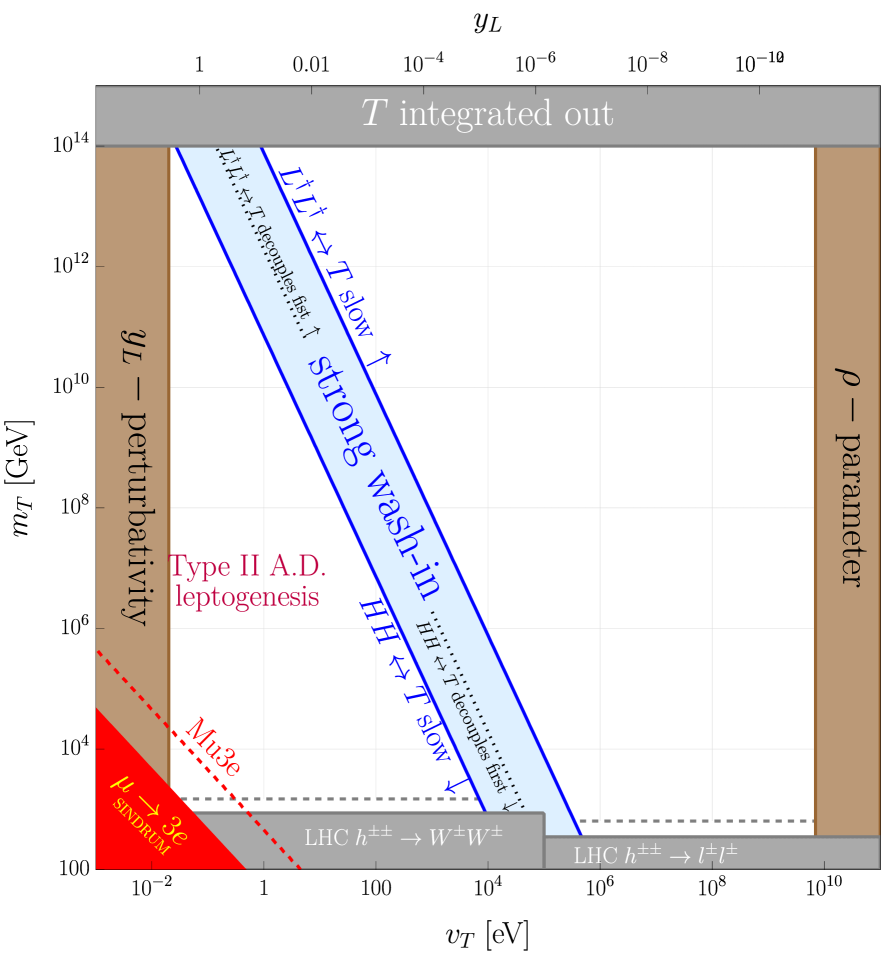
Figure 3: Summary of terrestrial limits on the Type II Seesaw mechanism from section 2.2. Straight line show current constraints and colored dashed lines refer to projected future limits. In order to show the range of $y_{L}$ on the upper axis we assumed a fiducial neutrino mass of $0.05\text{\,}\mathrm{eV}$ for reference. The blue band depicts the “strong wash-in” regime for Leptogenesis defined in Eq. (5.15). The “weak wash-in” regime is situated to the left and to the right of the blue band. In the left part of the plot labeled “Type II A.D. Leptogenesis” the scenario of Refs. Refs. [51, 52, 53, 54] is operative. For $m_{T}>\mathcal{O}(${10}^{14}\text{\,}\mathrm{GeV}$)$ the triplet would be too heavy to be in the thermal bath at the time the reactions from the lepton number violating Weinberg operator decouple, which will be discussed in section 6.

The Boltzmann equations from Ref. [44] are translated to the notation of Refs. [234, 62] to read in a Majoron background

$$\frac{\text{d}}{\text{d}\ln{(T)}}\left(\frac{\mu_{L}}{T}\right) =\frac{\Gamma_{L}^{\text{av.}}}{H(T)}\left(2\frac{\mu_{L}}{T}+\frac{\mu_{T}}{T}\right),$$ (5.5)

$$\frac{\text{d}}{\text{d}\ln{(T)}}\left(\frac{\mu_{H}}{T}\right) =\frac{\Gamma_{H}^{\text{av.}}}{H(T)}\left(2\frac{\mu_{H}}{T}-\frac{\mu_{T}}{T}-\frac{\dot{\theta}}{T}\right),$$ (5.6)

$$\frac{\text{d}}{\text{d}\ln{(T)}}\left(\frac{\mu_{T}}{T}\right) =\frac{1}{6}\frac{\Gamma_{L}^{\text{av.}}}{H(T)}\left(2\frac{\mu_{L}}{T}+\frac{\mu_{T}}{T}\right)-\frac{1}{3}\frac{\Gamma_{H}^{\text{av.}}}{H(T)}\left(2\frac{\mu_{H}}{T}-\frac{\mu_{T}}{T}-\frac{\dot{\theta}}{T}\right),$$ (5.7)

and here we defined the total chemical potential $\mu_{L}$

$$\mu_{L}=3\mu_{L_{i}},$$ (5.8)

in terms of the chemical potential of each generation $\mu_{L_{i}}$. We further dropped the contribution from the scattering terms as they are subdominant at $T=m_{T}$ for small couplings. Moreover there is no contribution from $CP$-violating out-of-equilibrium decays, since we work with a single generation of triplets. Here the $CP$ conserving tree level decay rates read [44]

$$\sum_{i}\Gamma_{L_{i}} \equiv\Gamma\left(T\rightarrow\sum_{i}L_{i}^{\dagger}L_{i}^{\dagger}\right)=\text{Tr}(|y_{L}|^{2})\frac{m_{T}}{16\pi}=\frac{\sum_{i}m_{\nu_{i}}^{2}}{8\pi v_{T}^{2}}m_{T},$$ (5.9)

$$\Gamma_{H} \equiv\Gamma\left(T\rightarrow HH\right)=\frac{\lambda_{\sigma HT}^{2}v_{\sigma}^{2}}{16\pi m_{T}}=\frac{v_{T}^{2}}{4\pi v_{H}^{4}}m_{T}^{3},$$ (5.10)

where we ignored the phase space suppression from the SM Higgs mass. The thermally averaged decay rates in the Maxwell Boltzmann approximation are found to be

$$\Gamma_{L}^{\text{av.}} \equiv\sum_{i}\frac{\text{K}_{1}(z)}{\text{K}_{2}(z)}\frac{\Sigma_{T}^{\text{eq.}}}{Y_{L_{i}}^{\text{eq.}}}\Gamma_{L_{i}},$$ (5.11)

$$\Gamma_{H}^{\text{av.}} \equiv\frac{\text{K}_{1}(z)}{\text{K}_{2}(z)}\frac{\Sigma_{T}^{\text{eq.}}}{Y_{H}^{\text{eq.}}}\Gamma_{H},$$ (5.12)

in terms of the modified Bessel function of the first (second) kind $\text{K}_{1}(z)\;\left(\text{K}_{2}(z)\right)$ and $z\equiv m_{T}/T$. One can understand the effect of the thermal average from the following expression

$$\Gamma_{i}^{\text{av.}}\simeq\frac{3}{2}\Gamma_{i}\begin{cases}\left(\frac{m_{T}}{T}\right)\quad&\text{for}\quad T\gg m_{T},\\ \sqrt{\frac{\pi}{2}}\left(\frac{m_{T}}{T}\right)^{\frac{3}{2}}e^{-\frac{m_{T}}{T}}\quad&\text{for}\quad T\ll m_{T},\end{cases}\quad\text{for}\quad i=L,H.$$ (5.13)

In Eq. (5.5) the contribution of $\dot{\theta}$ cancels out between $L$ and $T$ and hence the inverse $LL\rightarrow T^{\dagger}$ can not produce a chemical potential for either $T$ or $L$. The subsequent equation Eq. (5.6) on the other hand involves $T$ and $H$, where $\mu_{H}$ does not get shifted, since $H$ carries no lepton number. Consequently the $\dot{\theta}$ dependence does not cancel and the reaction $HH\rightarrow T$ can produce a chemical potential $\mu_{T}\sim\dot{\theta}$ that is then transmitted to $\mu_{L}$ via the decay $T\rightarrow L^{\dagger}L^{\dagger}$. This is only possible due to the fact that $T$ is not self conjugate, and can therefore have its own asymmetry described by the Boltzmann equation Eq. (5.7). An efficient production of lepton asymmetry therefore requires both rates $\Gamma_{H}^{\text{av.}}$ and $\Gamma_{L}^{\text{av.}}$ to be fast at $T=m_{T}$. This is not surprising, because “wash-in” Leptogenesis [58] requires the rates that “wash-out” the asymmetry produced in the conventional out-of-equilibrium decay scenario to be fast, and for scalar triplets it is well known, that “wash-out” is only efficient, if both rates are in equilibrium [44]. The decays and inverse decays reach their maximum at $T=m_{T}$ (see Fig. 4), and hence for strong washout we impose the conditions

$$K_{L,H}\equiv\frac{\Gamma_{L,H}^{\text{av.}}}{H(T)}\Big{|}_{T=m_{T}}\geq 1,$$ (5.14)

which imply that

$$$8.5\text{\,}\mathrm{keV}$\sqrt{\frac{$1\text{\,}\mathrm{TeV}$}{m_{T}}}<v_{T}<$277\text{\,}\mathrm{keV}$\sqrt{\frac{$1\text{\,}\mathrm{TeV}$}{m_{T}}}\sqrt{\frac{\overline{m}_{\nu}^{2}}{$2.65\text{\times}{10}^{-3}\text{\,}{\mathrm{eV}}^{2}$}}.$$ (5.15)

We call this the “strong wash-in” regime, and depicted it as a blue band in Fig. 3. One can analytically approximate the temperatures at which the processes come into thermal equilibrium

$$T_{L}^{\text{EQ}} \simeq$2.3\text{\,}\mathrm{TeV}$\left(\frac{m_{T}}{$1\text{\,}\mathrm{TeV}$}\right)^{\frac{2}{3}}\left(\frac{$100\text{\,}\mathrm{keV}$}{v_{T}}\right)^{\frac{2}{3}}\left(\frac{\overline{m}_{\nu}^{2}}{$2.65\text{\times}{10}^{-3}\text{\,}{\mathrm{eV}}^{2}$}\right)^{\frac{1}{3}},$$ (5.16)

$$T_{H}^{\text{EQ}} \simeq$6.1\text{\,}\mathrm{TeV}$\left(\frac{m_{T}}{$1\text{\,}\mathrm{TeV}$}\right)^{\frac{4}{3}}\left(\frac{v_{T}}{$100\text{\,}\mathrm{keV}$}\right)^{\frac{2}{3}}.$$ (5.17)

In order for Leptogenesis to proceed in the strong wash-in regime, we have to additionally ensure that the rates equilibrate before the critical temperature $T_{c}$ [62], at which the sphaleron transitions decouple [235]

$$T_{c}\simeq$130\text{\,}\mathrm{GeV}$.$$ (5.18)

From the conditions $T_{L,H}^{\text{EQ}}>T_{c}$ we obtain

$$$308\text{\,}\mathrm{eV}$\left(\frac{$1\text{\,}\mathrm{TeV}$}{m_{T}}\right)^{2}<v_{T}<$7.6\text{\,}\mathrm{MeV}$\left(\frac{m_{T}}{$1\text{\,}\mathrm{TeV}$}\right)\sqrt{\frac{\overline{m}_{\nu}^{2}}{$2.65\text{\times}{10}^{-3}\text{\,}{\mathrm{eV}}^{2}$}},$$ (5.19)

and these inequalities are always satisfied, when we impose the parameter range in Eq. (5.15) for the strong wash-in together with the lower bounds on $m_{T}$ from Eq. (2.17) and Eq. (2.18). Also note that since $T_{L,H}^{\text{EQ}}>m_{T}$, equilibration below $T_{c}$ would imply $m_{T}<T_{c}=$130\text{\,}\mathrm{GeV}$$, which is ruled out by the previously mentioned LHC searches.

The analytical expressions for the freeze-out temperature with $1\ll K_{L,H}<10^{4}$ are estimated to be (see section 6 of Ref. [236])

$$T_{L}^{\text{FO}} \simeq\frac{m_{T}}{5\sqrt{\log\left(\frac{9\sqrt{\frac{5}{2}}M_{\text{Pl}}\overline{m}_{\nu}^{2}}{32\pi^{2}\sqrt{g_{\rho}(T_{L}^{\text{FO}})}m_{T}v_{T}^{2}}\right)}},$$ (5.20)

$$T_{H}^{\text{FO}} \simeq\frac{m_{T}}{5\sqrt{\log\left(\frac{9\sqrt{\frac{5}{2}}M_{\text{Pl}}m_{T}v_{T}^{2}}{16\pi^{2}\sqrt{g_{\rho}(T_{H}^{\text{FO}})}v_{H}^{4}}\right)}}.$$ (5.21)

Here due to weak logarithmic dependence on the model parameters we find that

$$T_{L,H}^{\text{FO}}=\mathcal{O}\left(\frac{m_{T}}{10}\right).$$ (5.22)

Note that the above expressions are just used to provide some analytical intuition. All figures will be plotted using the numerically determined freeze-out temperatures.

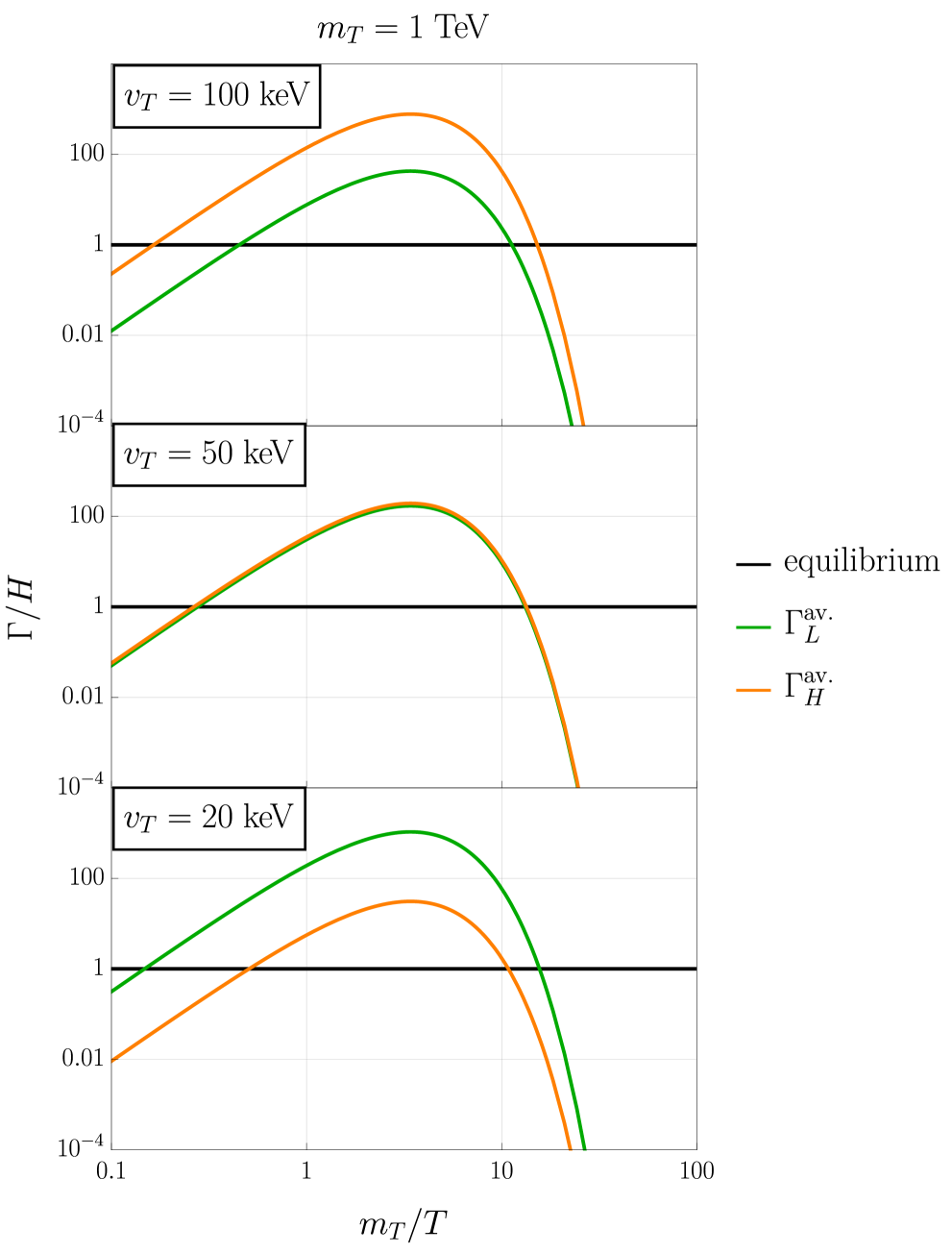
Figure 4: Rates for the processes $L^{\dagger}L^{\dagger}\leftrightarrow T$ (green) and $HH\leftrightarrow T$ (orange) normalized to the Hubble rate as a function of $m_{T}$ over temperature. For constant $m_{T}$ the values of $v_{T}$ were varied such that $L^{\dagger}L^{\dagger}\leftrightarrow T$ decouples after (upper panel), at the same time as (middle panel) or before (lower panel) $HH\leftrightarrow T$.

The reaction involving $L$ freezes out before the inverse decays to $H$ as long as

$$v_{T}>$48\text{\,}\mathrm{keV}$\left(\frac{\overline{m}_{\nu}^{2}}{$2.65\text{\times}{10}^{-3}\text{\,}{\mathrm{eV}}^{2}$}\right)^{\frac{1}{4}}\sqrt{\frac{$1\text{\,}\mathrm{TeV}$}{m_{T}}},$$ (5.23)

and a numerical example that demonstrates, which rate decouples first was displayed in Fig. 4. We also show the regions in the $m_{T}$ versus $v_{T}$ parameter plane, in which each of the rates decouples first in Fig. 3.

The original Boltzmann equations from Ref. [44] satisfy a sum rule

$$2\Delta_{T}+\Delta_{H}-\Delta_{L}=0,$$ (5.24)

which corresponds to the following condition on the chemical potentials

$$6\mu_{T}+2\mu_{H}-\mu_{L}=0,$$ (5.25)

and one can check that this is satisfied by Eqns. (5.5)-(5.7). This statement is nothing more than hypercharge conservation [44] for the triplet and its decay products. Our analysis treats the lepton number violating processes on the same footing as the other spectator processes [58], which redistribute the lepton asymmetry (see Ref. [237]), and therefore the previously mentioned sum rule is included in the conservation of the total hypercharge of the plasma

$$3\left(\mu_{Q_{i}}+\mu_{u_{i}}-\mu_{d_{i}}-\mu_{L_{i}}-\mu_{e_{i}}\right)+6\mu_{T}+2\mu_{H}=0,$$ (5.26)

where we remind the reader that $3\mu_{L_{i}}=\mu_{L}$. We take all Standard Model Yukawa interactions to be fast, which is accurate below about ${10}^{5}\text{\,}\mathrm{GeV}$ [238], and include the equilibrated interactions of the triplet

$$\mu_{T}+2\mu_{L_{i}}=0,\quad\mu_{T}-2\mu_{H}+\dot{\theta}=0.$$ (5.27)

The sphaleron redistribution coefficient can be read off from

$$\mu_{B_{i}}=-\frac{14}{51}\dot{\theta}=\frac{28}{61}\mu_{(B-L)_{i}},$$ (5.28)

and its value of $28/61$ is larger than the sphaleron redistribution coefficient of $28/79$ for models without a thermalized triplet scalar. Note that the value of this coefficient changes for models in which the Majoron is identified with a QCD axion due to its direct coupling to QCD sphalerons, see e.g. [64]. In general the resulting baryon asymmetry can be parameterized as

$$\Delta_{B}=\frac{7}{153}\text{Min}\left[1,\frac{\Gamma_{L}^{\text{av.}}}{H(T)}\right]\text{Min}\left[1,\frac{\Gamma_{H}^{\text{av.}}}{H(T)}\right]\left(\frac{T}{v_{\sigma}}\right)^{2}Y_{\theta}\Big{|}_{T=\tilde{T}},$$ (5.29)

with

$$\tilde{T}\equiv\begin{cases}\text{Max}\left[T_{L}^{\text{FO}},T_{H}^{\text{FO}}\right]\quad&\text{for}\;K_{L}\geq 1\land K_{H}\geq 1\land\text{Max}\left[T_{L}^{\text{FO}},T_{H}^{\text{FO}}\right]>T_{c},\\ T_{L}^{\text{FO}}\quad&\text{for}\;K_{L}\geq 1\land K_{H}<1\land T_{L}^{\text{FO}}>T_{c},\\ T_{H}^{\text{FO}}\quad&\text{for}\;K_{L}<1\land K_{H}\geq 1\land T_{H}^{\text{FO}}>T_{c},\\ T_{c}\quad&\text{else}.\end{cases}$$ (5.30)

In the above $\tilde{T}$ is determined by which process decouples first. If the rates involving the triplets never thermalize, or only decouple below the sphaleron decoupling at $T_{c}$, the sphalerons freeze-out first and hence $\tilde{T}=T_{c}$. Otherwise the condition in Eq. (5.23) allows one to determine whether $T_{L}^{\text{FO}}$ or $T_{H}^{\text{FO}}$ is larger. We can deduce from Eq. (5.15) that either $\Gamma_{L}^{\text{av.}}$ or $\Gamma_{H}^{\text{av.}}$, but not both, can be slow. Therefore the asymmetry can only depend on at most a single factor of either $\Gamma_{L}^{\text{av.}}/H(T)$ or $\Gamma_{H}^{\text{av.}}/H(T)$.

Note that spontaneous Leptogenesis in a Majoron background is not affected by the triplet’s gauge interactions, unlike the conventional out-of-equilibrium decay scenario: There the source term for the lepton asymmetry is $\varepsilon_{L}(\Sigma_{T}-\Sigma_{T}^{\text{eq.}})$, where $\varepsilon_{L}$ is the amount of $CP$ violation per triplet decay corresponding to the second Sakharov condition, and $\Sigma_{T}-\Sigma_{T}^{\text{eq.}}$ is the deviation from equilibrium encoded in the third Sakharov condition. One expects that the electroweak gauge annihilations $\overline{T}T\rightarrow WW,WY,YY$ keep $\Sigma_{T}$ closer to $\Sigma_{T}^{\text{eq.}}$ reducing the efficiency of the conventional Leptogenesis; however Ref. [44] showed that in the strong washout regime the decays and inverse decays actually are the dominant processes thermalizing the triplet. In spontaneous Leptogenesis the source term is instead given by $\dot{\theta}$, which breaks $CP$ and $CPT$ spontaneously. Therefore the third Sakharov condition and the corresponding out-of-equilibrium conditions are not required. Furthermore gauge annihilations only act on the symmetric component $\Sigma_{T}$, but we use the inverse decays $HH\leftrightarrow T$ to generate the asymmetric component $\Delta_{T}$, which stores the asymmetry, before releasing it via decays to leptons.

5.1.1 Strong Wash-In

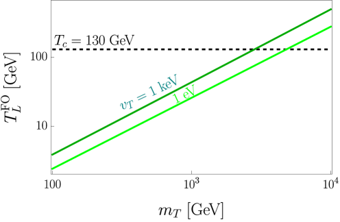
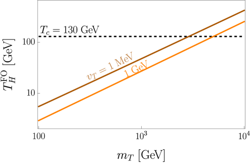
Figure 5: Numerically determined freeze-out temperatures of $\Gamma_{L}^{\text{av.}}$ (left) and $\Gamma_{H}^{\text{av.}}$ (right) as a function of $m_{T}$ for different choices of $v_{T}=\{$1\text{\,}\mathrm{eV}$,\;$1\text{\,}\mathrm{keV}$,\;$1\text{\,}\mathrm{MeV}$,\;$1\text{\,}\mathrm{GeV}$\}$. Note that the choices for $v_{T}$ not depicted in each respective plot do not lead to successful thermalization.

In order to develop some intuition for the required parameter space we proceed with analytical estimates: Saturating the inequality in Eq. (5.23) means that $\Gamma_{L}^{\text{av.}}$ and $\Gamma_{H}^{\text{av.}}$ decouple around the same time, and as long as Eq. (5.15) is satisfied we can work in the strong wash-in regime

$$\Delta_{B}\simeq\frac{7}{153}\left(\frac{\tilde{T}}{v_{\sigma}}\right)^{2}Y_{\theta}.$$ (5.31)

Since the freeze-out of the inverse decays typically happens at the temperature given by Eq. (5.22), we deduce that these processes decouple above $T_{c}$ for $m_{T}>\mathcal{O}(10)T_{c}=$1.3\text{\,}\mathrm{TeV}$$. It is important to emphasize that this is just a rough estimate for the sake of analytical understanding. In Fig. 5 we plot the numerically determined freeze-out temperature $T_{L,H}^{\text{FO}}$ for both rates $\Gamma_{L,H}^{\text{av.}}$, and find in each case that decoupling actually occurs above $T_{c}$ for somewhat larger values of $m_{T}\simeq(3-5)\;\text{TeV}$. Our previous estimate allows us to write a simplified approximate expression for the decoupling temperature

$$\tilde{T}\simeq\begin{cases}\frac{m_{T}}{\mathcal{O}(10)}\quad&\text{for}\quad m_{T}>$1.3\text{\,}\mathrm{TeV}$,\\ T_{c}\quad&\text{for}\quad m_{T}<$1.3\text{\,}\mathrm{TeV}$.\end{cases}$$ (5.32)

Trading $Y_{\theta}$ for $m_{j}$ we find that

$$\Delta_{B}\simeq 8.76\times 10^{-11}\left(\frac{${10}^{8}\text{\,}\mathrm{GeV}$}{v_{\sigma}}\right)^{2}\begin{cases}\left(\frac{m_{T}}{$100\text{\,}\mathrm{TeV}$}\right)^{2}\left(\frac{$1\text{\,}\mathrm{eV}$}{m_{j}}\right)\quad&\text{for}\quad m_{T}>$1.3\text{\,}\mathrm{TeV}$,\\ \left(\frac{$0.2\text{\,}\mathrm{meV}$}{m_{j}}\right)\quad&\text{for}\quad m_{T}<$1.3\text{\,}\mathrm{TeV}$.\end{cases}$$ (5.33)

Here we need $v_{T}\simeq$4.8\text{\,}\mathrm{keV}$$ for $m_{T}=$100\text{\,}\mathrm{TeV}$$ from Eq. (5.23).

5.1.2 Weak Wash-In

Next we show an analytical expression for the case when one of the rates is suppressed compared to the other

$$\Delta_{B}\simeq\frac{7}{153}\left(\frac{\tilde{T}}{v_{\sigma}}\right)^{2}Y_{\theta}\begin{cases}\frac{\Gamma_{L}^{\text{av.}}}{H}\Big{|}_{\tilde{T}}\quad\text{for}\quad v_{T}>$277\text{\,}\mathrm{keV}$\sqrt{\frac{$1\text{\,}\mathrm{TeV}$}{m_{T}}}\sqrt{\frac{\overline{m}_{\nu}^{2}}{$3\text{\times}{10}^{-3}\text{\,}{\mathrm{eV}}^{2}$}},\\ \frac{\Gamma_{H}^{\text{av.}}}{H}\Big{|}_{\tilde{T}}\quad\text{for}\quad v_{T}<$8.5\text{\,}\mathrm{keV}$\sqrt{\frac{$1\text{\,}\mathrm{TeV}$}{m_{T}}},\end{cases}$$ (5.34)

where $\tilde{T}$ is still given by Eq. (5.32). In case $\Gamma_{L}^{\text{av.}}$ never thermalizes we obtain

$$\Delta_{B}\simeq 8.76\times 10^{-11}\left(\frac{${10}^{8}\text{\,}\mathrm{GeV}$}{v_{\sigma}}\right)^{2}\sqrt{\frac{\overline{m}_{\nu}^{2}}{$2.65\text{\times}{10}^{-3}\text{\,}{\mathrm{eV}}^{2}$}}\begin{cases}\left(\frac{m_{T}}{$10\text{\,}\mathrm{TeV}$}\right)\left(\frac{$100\text{\,}\mathrm{keV}$}{v_{T}}\right)^{2}\left(\frac{$2.7\text{\,}\mathrm{meV}$}{m_{j}}\right),\\ \left(\frac{m_{T}}{$1\text{\,}\mathrm{TeV}$}\right)^{\frac{5}{2}}\left(\frac{$500\text{\,}\mathrm{keV}$}{v_{T}}\right)^{2}\left(\frac{$71\text{\,}\mathrm{\SIUnitSymbolMicro eV}$}{m_{j}}\right).\end{cases}$$ (5.35)

If instead $\Gamma_{H}^{\text{av.}}$ never thermalizes we find

$$\Delta_{B}\simeq 8.76\times 10^{-11}\left(\frac{${10}^{8}\text{\,}\mathrm{GeV}$}{v_{\sigma}}\right)^{2}\begin{cases}\left(\frac{m_{T}}{$10\text{\,}\mathrm{TeV}$}\right)^{3}\left(\frac{v_{T}}{$1\text{\,}\mathrm{keV}$}\right)^{2}\left(\frac{$0.5\text{\,}\mathrm{meV}$}{m_{j}}\right),\\ \left(\frac{m_{T}}{$1\text{\,}\mathrm{TeV}$}\right)^{\frac{9}{2}}\left(\frac{v_{T}}{$5\text{\,}\mathrm{keV}$}\right)^{2}\left(\frac{$81\text{\,}\mathrm{\SIUnitSymbolMicro eV}$}{m_{j}}\right).\end{cases}$$ (5.36)

One should be careful with the above expressions for $m_{T}<$1.3\text{\,}\mathrm{TeV}$$ as they non-linearly depend on $m_{T}$ due to the Boltzmann suppression $e^{-m_{T}/T_{c}}$ (see Eq. (5.13)).

5.2 Constraints

Overall it is important to emphasize, that our Leptogenesis scenario can in principle work with all triplet masses above the collider limits in Eqns. (2.17)-(2.18). More specifically we can accommodate TeV-scale triplets in reach of present and next generation collider experiments.

The backreaction of the fermionic asymmetry generation on the Majoron rotation is negligible as long as $T\ll v_{\sigma}$ [63], so the condensate persists until later times and can source the dark matter abundance. Here this constraint implies $\tilde{T}\ll v_{\sigma}$ so that

$$v_{\sigma}\gg T_{c}\quad\text{for}\quad m_{T}<$1.3\text{\,}\mathrm{TeV}$,$$ (5.37)

as well as

$$m_{T}\ll 10v_{\sigma}\quad\text{for}\quad m_{T}>$1.3\text{\,}\mathrm{TeV}$.$$ (5.38)

In order for our assumption of radiation domination to be valid, we have to demand the kinetic energy of the Majoron rotation is subdominant to the energy density of the thermal plasma at least at the time of asymmetry production

$$\frac{\dot{\theta}^{2}v_{\sigma}^{2}}{2}<\frac{\pi^{2}}{30}g_{\rho}(\tilde{T})\tilde{T}^{4},$$ (5.39)

which corresponds to an upper limit on $Y_{\theta}$. Here we follow the treatment of Ref. [62], where $Y_{\theta}=\dot{\theta}v_{\sigma}^{2}/s$ is fixed to reproduce the baryon asymmetry. Using this together with the analytical result from the strong wash-in regime in Eq. (5.33) we find that

$$v_{\sigma}<\begin{cases}$3\text{\times}{10}^{11}\text{\,}\mathrm{GeV}$\left(\frac{m_{T}}{$10\text{\,}\mathrm{TeV}$}\right)\quad&\text{for}\quad m_{T}>$1.3\text{\,}\mathrm{TeV}$,\\ $1.2\text{\times}{10}^{10}\text{\,}\mathrm{GeV}$\quad&\text{for}\quad m_{T}<$1.3\text{\,}\mathrm{TeV}$,\end{cases}$$ (5.40)

where we used $g_{\rho}(\tilde{T})=106.75=g_{s}(\tilde{T})$. For the more suppressed asymmetry production from weak wash-in with a slow $\Gamma_{L}^{\text{inv.}}$ discussed in Eq. (5.35) we find that

$$v_{\sigma}<\left(\frac{\overline{m}_{\nu}^{2}}{$2.65\text{\times}{10}^{-3}\text{\,}{\mathrm{eV}}^{2}$}\right)\begin{cases}$2.2\text{\times}{10}^{10}\text{\,}\mathrm{GeV}$\left(\frac{$100\text{\,}\mathrm{keV}$}{v_{T}}\right)^{2}\quad&\text{for}\quad m_{T}>$1.3\text{\,}\mathrm{TeV}$,\\ $4.5\text{\times}{10}^{9}\text{\,}\mathrm{GeV}$\left(\frac{m_{T}}{$1\text{\,}\mathrm{TeV}$}\right)^{\frac{5}{2}}\left(\frac{$500\text{\,}\mathrm{keV}$}{v_{T}}\right)^{2}\quad&\text{for}\quad m_{T}<$1.3\text{\,}\mathrm{TeV}$,\end{cases}$$ (5.41)

and for the case with a slow $\Gamma_{H}^{\text{av.}}$ from Eq. (5.36) we deduce

$$v_{\sigma}<\begin{cases}$4\text{\times}{10}^{9}\text{\,}\mathrm{GeV}$\left(\frac{m_{T}}{$10\text{\,}\mathrm{TeV}$}\right)^{2}\left(\frac{v_{T}}{$1\text{\,}\mathrm{keV}$}\right)^{2}\quad&\text{for}\quad m_{T}>$1.3\text{\,}\mathrm{TeV}$,\\ $5\text{\times}{10}^{9}\text{\,}\mathrm{GeV}$\left(\frac{m_{T}}{$1\text{\,}\mathrm{TeV}$}\right)^{\frac{9}{2}}\left(\frac{v_{T}}{$5\text{\,}\mathrm{keV}$}\right)^{2}\quad&\text{for}\quad m_{T}<$1.3\text{\,}\mathrm{TeV}$.\end{cases}$$ (5.42)

Our calculation assumed that $\theta$ is a slowly varying background field. In order for $\theta$ to remain approximately constant over the time scale of thermal processes $1/T$ we impose that [64]

$$\dot{\theta}<\tilde{T},$$ (5.43)

and proceed in a similar vein to the previous limit. For all cases we find that the $v_{\sigma}$ dependence divides out. In the strong wash-in regime with $Y_{\theta}$ fixed via the observed baryon asymmetry the adiabaticity condition is always satisfied. In the weak wash-in regime with a slow $\Gamma_{L}^{\text{av.}}$ discussed in Eq. (5.35) we obtain an upper limit on $v_{T}$ of

$$v_{T}<\sqrt{\frac{\overline{m}_{\nu}^{2}}{$2.65\text{\times}{10}^{-3}\text{\,}{\mathrm{eV}}^{2}$}}\begin{cases}$163\text{\,}\mathrm{MeV}$\sqrt{\frac{$10\text{\,}\mathrm{TeV}$}{m_{T}}}\quad&\text{for}\quad m_{T}>$1.3\text{\,}\mathrm{TeV}$,\\ $1\text{\,}\mathrm{GeV}$\left(\frac{m_{T}}{$1\text{\,}\mathrm{TeV}$}\right)^{\frac{5}{4}}\quad&\text{for}\quad m_{T}<$1.3\text{\,}\mathrm{TeV}$,\end{cases}$$ (5.44)

and for the case with a slow $\Gamma_{H}^{\text{av.}}$ from Eq. (5.36) we find a lower limit on $v_{T}$ of

$$v_{T}>\begin{cases}$1.5\text{\,}\mathrm{eV}$\sqrt{\frac{$10\text{\,}\mathrm{TeV}$}{m_{T}}}\quad&\text{for}\quad m_{T}>$1.3\text{\,}\mathrm{TeV}$,\\ $2.3\text{\,}\mathrm{eV}$\left(\frac{$1\text{\,}\mathrm{TeV}$}{m_{T}}\right)^{\frac{9}{4}}\quad&\text{for}\quad m_{T}<$1.3\text{\,}\mathrm{TeV}$.\end{cases}$$ (5.45)

By comparing these bounds with the definition of the weak wash-in regime in Eq. (5.15), one can deduce that they do not impose significant constraints on our parameter space.

The authors of Ref. [237] argued that one should take

$$|\dot{\theta}|<m_{T},$$ (5.46)

to avoid Bose condensation of the triplet scalar. From Eq. (5.43) we see, that $|\dot{\theta}|$ is bounded from above by $\tilde{T}$, whose order of magnitude can be found in Eq. (5.32), and this evinces that Bose condensation of the triplet does not occur.

5.3 Oscillating radial mode

So far we have assumed that the vev of $\sigma$ is stabilized at its present day value $v_{\sigma}$ during Leptogenesis. For a Majoron rotation from the Affleck-Dine mechanism in section 3.2.1 we have to ensure that the dynamics at the beginning of the radial oscillations, when the radial mode takes a large field value $S_{i}\gg v_{\sigma}$, do not affect these results. Processes like $SHH\leftrightarrow T$ could modify the triplet asymmetry production at early time and its rate scales as

$$\Gamma(SHH\leftrightarrow T)\simeq\frac{\lambda_{\sigma HT}^{2}}{16\pi}\frac{S^{2}}{T},$$ (5.47)

where for a quartic potential with $S\sim 1/a$ we find $\Gamma(SHH\leftrightarrow T)/H(T)\sim 1/T$ during radiation domination, implying that this rate is IR dominated. The large field value never affects Leptogenesis, if the reaction involving it only equilibrates after $h_{\sigma}$ has settled to its true minimum at $v_{\sigma}$, which for a quartic potential occurs at

$$T_{\text{min}}=\frac{v_{\sigma}}{S_{i}}T_{\text{osc.}},$$ (5.48)

where $T_{\text{osc.}}$ was defined in Eq. (3.24). This implies the condition

$$v_{T}<$11\text{\,}\mathrm{MeV}$\left(\frac{$1\text{\,}\mathrm{TeV}$}{m_{T}}\right)^{2}\left(\frac{v_{\sigma}}{${10}^{9}\text{\,}\mathrm{GeV}$}\right)^{\frac{3}{2}}\left(\frac{T_{\text{osc.}}}{${10}^{15}\text{\,}\mathrm{GeV}$}\right)^{\frac{3}{2}}\left(\frac{M_{\text{Pl.}}}{S_{i}}\right).$$ (5.49)

Here we assume that the production temperature of the baryon asymmetry $\tilde{T}$ defined in Eq. (5.32) is below $T_{\text{min}}$, which implies

$$\tilde{T}<${10}^{5}\text{\,}\mathrm{GeV}$\left(\frac{v_{\sigma}}{${10}^{9}\text{\,}\mathrm{GeV}$}\right)\left(\frac{M_{\text{Pl.}}}{S_{i}}\right)\left(\frac{T_{\text{osc.}}}{${10}^{15}\text{\,}\mathrm{GeV}$}\right).$$ (5.50)

If $m_{T}>$1.3\text{\,}\mathrm{TeV}$$ we can deduce from Eq. (5.32) that

$$m_{T}<${10}^{6}\text{\,}\mathrm{GeV}$\left(\frac{v_{\sigma}}{${10}^{9}\text{\,}\mathrm{GeV}$}\right)\left(\frac{M_{\text{Pl.}}}{S_{i}}\right)\left(\frac{T_{\text{osc.}}}{${10}^{15}\text{\,}\mathrm{GeV}$}\right).$$ (5.51)

Thus we can sequester the generation of the rotation in the Affleck Dine scenario at the large temperature $T_{\text{osc.}}$ from the generation of the baryon asymmetry at the much lower temperature $\tilde{T}$.

6 High scale Leptogenesis (triplet not in the thermal bath)

Here we comment on the features of the scenario where the triplet is heavy enough to be integrated out at all times. In case the triplet is not part of the thermal bath, we can work in the effective operator limit making use of the Weinberg operator. Consequently one would expect that Leptogenesis in this regime is not sensitive to the UV completion of the Weinberg operator in a similar manner to the scenarios discussed in Refs. [59, 60, 165, 64, 84, 62, 146, 66]. The Boltzmann equation for the lepton chemical potential reads

$$\frac{\text{d}}{\text{d}\ln{(T)}}\left(\frac{\mu_{L}}{T}\right)=\frac{\Gamma_{W}}{H(T)}\left(\frac{\mu_{L}}{T}-\frac{\dot{\theta}}{T}\right),$$ (6.1)

but here we will not discuss Leptogenesis further as it has been covered in a wide array of literature before [59, 60, 165, 64, 84, 62, 146, 66]. Instead we comment on the implications for the Type II Seesaw. Here the rate for the process $LL\leftrightarrow HH$ and all processes related by crossing symmetry is

$$\Gamma_{W}\equiv\Gamma\left(LL\leftrightarrow HH\right)=\frac{1}{4\pi^{3}}\frac{\sum_{i}m_{\nu_{i}}^{2}}{v_{H}^{4}}T^{3},$$ (6.2)

which freezes out at

$$T_{W}^{\text{FO}}\simeq$2.41\text{\times}{10}^{14}\text{\,}\mathrm{GeV}$\left(\frac{$2.65\text{\times}{10}^{-3}\text{\,}{\mathrm{eV}}^{2}$}{\overline{m_{\nu}}^{2}}\right).$$ (6.3)

For this estimate to be self-consistent we have to impose that the triplet is at least heavier than the freeze-out temperature

$$m_{T}>\mathcal{O}(${10}^{14}\text{\,}\mathrm{GeV}$),$$ (6.4)

which was depicted in Fig. 3. Such heavy triplet masses require large values of $v_{\sigma}$ to maintain the smallness of $v_{T}$ in Eq. (2.7) for perturbative values of $\lambda_{\sigma HT}<\sqrt{4\pi}$. We can use this to find a lower limit on the lepton number breaking scale of

$$v_{\sigma}>\frac{v_{T}}{\sqrt{4\pi}}\frac{m_{T}^{2}}{v_{H}^{2}}\simeq$5\text{\times}{10}^{13}\text{\,}\mathrm{GeV}$\left(\frac{v_{T}}{$1\text{\,}\mathrm{eV}$}\right)\left(\frac{m_{T}}{${10}^{14}\text{\,}\mathrm{GeV}$}\right)^{2}.$$ (6.5)

A distinction occurs when the radial mode of $\sigma$ develops a large initial field value as in the Affleck-Dine mechanism discussed in section 3.2.1. Because the Weinberg operator for the Type II Seesaw is sensitive to an insertion of this vev and hence its dynamics (see Fig. 2 and Eq. (2.6)), the rate for processes like $SLL\leftrightarrow HH$ changes to (see e.g. Ref. [65, 80])

$$\Gamma_{SW}\equiv\Gamma\left(SLL\leftrightarrow HH\right)=\frac{1}{4\pi^{3}}\frac{\sum_{i}m_{\nu_{i}}^{2}}{v_{H}^{4}}T^{3}\left(\frac{S}{v_{\sigma}}\right)^{2}=\Gamma_{W}\left(\frac{S}{v_{\sigma}}\right)^{2}.$$ (6.6)

For concreteness we assume a quartic potential for $\sigma$ so that during radiation domination

$$S(T)=S_{i}\frac{T}{T_{\text{osc.}}}.$$ (6.7)

Assuming that $S$ is already moving this process freezes out at

$$T_{SW}^{\text{FO}}=${10}^{8}\text{\,}\mathrm{GeV}$\left(\frac{$2.65\text{\times}{10}^{-3}\text{\,}{\mathrm{eV}}^{2}$}{\overline{m_{\nu}}^{2}}\right)\left(\frac{v_{\sigma}}{${10}^{10}\text{\,}\mathrm{GeV}$}\right)^{\frac{2}{3}}\left(\frac{M_{\text{Pl.}}}{S_{i}}\right)^{\frac{2}{3}}\left(\frac{T_{\text{osc.}}}{${10}^{14}\text{\,}\mathrm{GeV}$}\right)^{\frac{2}{3}},$$ (6.8)

and once can see that the $v_{\sigma}/S_{i}$ suppression lowers the freeze-out temperature. This could in principle allow for a smaller $m_{T}$, if we only require it to be absent from the plasma below $T_{SW}^{\text{FO}}$. Note however that the scenario with large $S_{i}$ faces strong constraints from dark radiation due to irreducible contribution from decays of the radial mode in Eq. (4.27). Requiring $\Delta N_{\text{eff.}}<0.17$ implies

$$v_{\sigma}<$2.5\text{\times}{10}^{12}\text{\,}\mathrm{GeV}$\left(\frac{T_{\text{osc.}}}{$6.5\text{\times}{10}^{15}\text{\,}\mathrm{GeV}$}\right)^{2}\left(\frac{M_{\text{Pl.}}}{S_{i}}\right),$$ (6.9)

where we used the largest possible $T_{\text{osc.}}$ from Eq. (3.25). Note that Leptogenesis in this regime is independent of $v_{T}$, but as we argued in Eq. (2.24) $v_{T}$ can not be too far below the eV-scale. If we use this information in Eq. (6.5), we find that

$$v_{\sigma}>$2.5\text{\times}{10}^{12}\text{\,}\mathrm{GeV}$\left(\frac{v_{T}}{$0.02\text{\,}\mathrm{eV}$}\right)\left(\frac{m_{T}}{$1.6\text{\times}{10}^{14}\text{\,}\mathrm{GeV}$}\right)^{2}.$$ (6.10)

On the one hand this example demonstrates that we can not lower the triplet mass much below the conventional upper limit in Eq. (6.4), and on the other hand we see that at best there is only a narrow allowed parameter window. The available parameter space is even further reduced once we include the other reactions producing Majorons from section 4.4.2. Together with the fact that high scale scenario is hard to test experimentally these arguments illustrate, why we de not consider the high-scale scenario in more detail.

7 Discussion

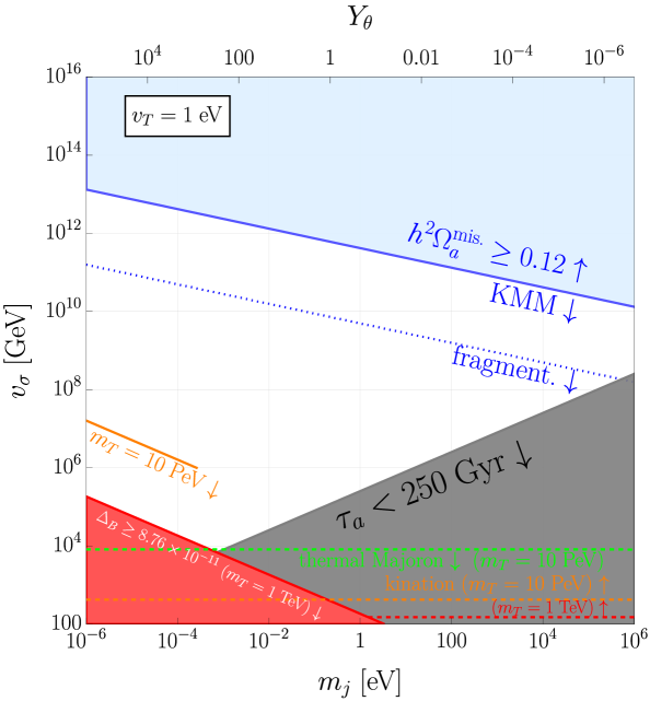
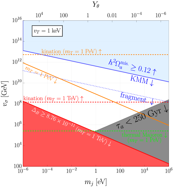
Figure 6: Parameter space for the cogenesis of the baryon asymmetry and dark matter relic abundance via kinetic misalignment in the plane spanned by the lepton number breaking scale $v_{\sigma}$ and the Majoron mass $m_{j}$ for $v_{T}=$1\text{\,}\mathrm{eV}$$ (upper panel) and $v_{T}=$1\text{\,}\mathrm{keV}$$ (lower panel). An explanation of all colored lines and regions is given section 7.

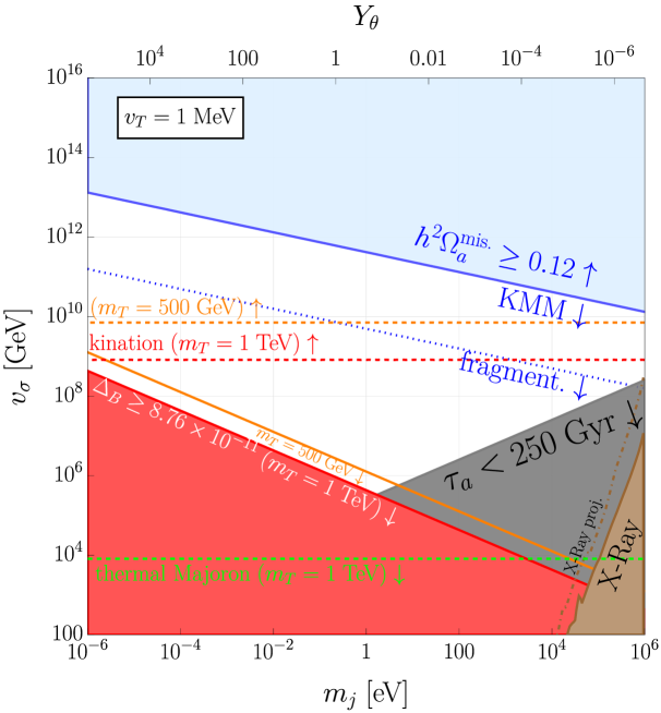
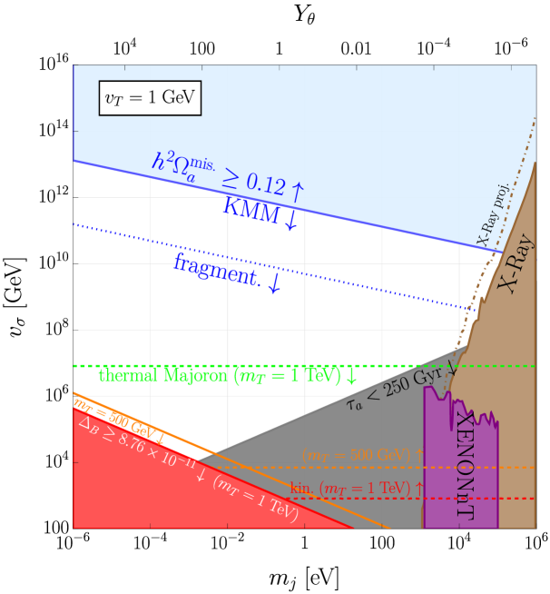
Figure 7: Parameter space for the cogenesis of the baryon asymmetry and dark matter relic abundance via kinetic misalignment in the plane spanned by the lepton number breaking scale $v_{\sigma}$ and the Majoron mass $m_{j}$ for $v_{T}=$1\text{\,}\mathrm{MeV}$$ (upper panel) and $v_{T}=$1\text{\,}\mathrm{GeV}$$ (lower panel). An explanation of all colored lines and regions is given section 7.

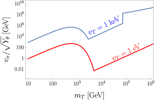
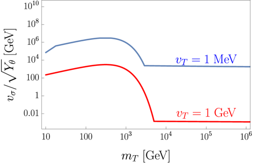
Figure 8: The required value of $v_{\sigma}/\sqrt{Y_{\theta}}$ for successful Leptogenesis from Eq. (5.29) as a function of $m_{T}$ for different values of $v_{T}=\{$1\text{\,}\mathrm{eV}$,\;$1\text{\,}\mathrm{keV}$,\;$1\text{\,}\mathrm{MeV}$,\;$1\text{\,}\mathrm{GeV}$\}$. In the left figure $\Gamma^{\text{av.}}_{H}$ is out of equilibrium, and in the right figure $\Gamma_{L}^{\text{av.}}$ is out of equilirbium. For a fixed $m_{T}$ the left plot can be mapped to the parameter space in Fig. 6, and the right plot can be translated to the parameter space in Fig. 7.

7.1 Parameter Space

We display our collection of predictions and constraints in the $v_{\sigma}$ versus $m_{j}$ parameter plane in Figs. 6-7, where we varied $v_{T}$ in steps of three orders of magnitude between $1\text{\,}\mathrm{eV}$ and $1\text{\,}\mathrm{GeV}$.

Let us first discuss the implications for dark matter: Here we also display the value of the Majoron yield $Y_{\theta}$ that is required for a given $m_{j}$ to explain the dark matter relic abundance via kinetic misalignment, see Eq. (4.7). For each point one can then check, if a given model from sections 3.2.1-3.2.2 can realize the required $Y_{\theta}$. For the Affleck-Dine scenario one can then also check, whether the constraint from the sequestering in Eq. (5.49) is satisfied. In all plots kinetic misalignment dominates over the conventional misalignment (see Eq. (4.8)) in the region below the blue line labeled “KMM $\downarrow$”. On this blue line the relic abundance is saturated by the usual misalignment contribution from Eq. (4.2), where we chose the post-inflationary lepton number breaking scenario with an patch-averaged initial misalignment angle of $\sqrt{\braket{\theta_{i}^{2}}}=2.1$ [173]. For smaller $\theta_{i}$ from the pre-inflationary scenario the relic abundance is fixed for larger $v_{\sigma}$. Below the dotted blue line labeled “fragment. $\downarrow$” the Majoron condensate fragments into higher momentum excitations as described in the discussion surrounding Eq. (4.9) from Ref. [178].

In the black area the dark matter lifetime from decays to neutrinos (Eq. (4.11)) or photons (Eq. (4.13)) is below $250\;\text{Gyr}$. We find that the photon decay mode requires larger $v_{T}$ of the order $\mathcal{O}($1\text{\,}\mathrm{GeV}$)$ to be relevant at all, which is close to the upper bound from electroweak precision observables in Eq. (2.23). Existing limits from X-Ray and gamma ray searches were displayed as brown regions and projected future limits as brown dot-dashed lines (consult Ref. [198] and references therein for details). From both panels in Fig 7 it can be deduced that the aforementioned limits only become relevant for $v_{T}>\mathcal{O}($1\text{\,}\mathrm{MeV}$)$, and they can dominate over the lifetime constraint for large $m_{j}$ if $v_{T}=\mathcal{O}($1\text{\,}\mathrm{GeV}$)$.

The direct detection limit from Majorons scattering off electrons obtained by the XENONnT [197] collaboration for an exposure of $1.16\;\text{ton}\times\text{year}$ was drawn in purple. For a larger exposure the exclusion limit would move upwards to larger $v_{\sigma}$. The lower panel in Fig. 7 reveals, that this limit also only matters for $v_{T}=\mathcal{O}($1\text{\,}\mathrm{GeV}$)$ together with $m_{j}=\mathcal{O}($10\text{\,}\mathrm{keV}$)$, $v_{\sigma}=\mathcal{O}(${10}^{6}\text{\,}\mathrm{GeV}$)$. The authors of Ref. [37] attempted to populate this parameter region via the freeze-in production of Majorons, which required an earlier electroweak phase transition together with an early matter dominated epoch.

Concerning dark radiation and hot dark matter our results indicate that the strongest limits come from the non-thermalization conditions in Eq. (4.23) and Eq. (4.29), which was drawn as a green line labeled “thermal Majoron $\downarrow$”. By comparing both equations one finds that the limit from scattering is stronger. From the lower panel in Fig. 7 it is clear that most of the parameter space for $v_{T}=\mathcal{O}($1\text{\,}\mathrm{GeV}$)$ would be ruled out by the Majoron thermalization. This finding mirrors the conclusions reached in Ref. [37], and was one of the reasons, why the authors of that reference considered early matter domination. Depending on the combination of $v_{T}$ and $m_{T}$ this constraint rules out $v_{\sigma}$ below $\mathcal{O}(${10}^{4}\text{\,}\mathrm{GeV}$)$-$\mathcal{O}(${10}^{7}\text{\,}\mathrm{GeV}$)$. We verified that the constraints from the dark radiation abundance encoded in $\Delta N_{\text{eff.}}$ and the limit on the hot dark matter abundance in Eq. (4.22) were subleading.

Next we discuss what conclusions can be drawn for Leptogenesis: For a given $m_{T}$ we showcase the line on which the observed value of the baryon asymmetry $\Delta_{B}=8.76\times 10^{-11}$ [38, 39] is reproduced by Eq. (5.29). Below this line the asymmetry is overproduced for the same $m_{T}$. In all plots we use the color red for $m_{T}=$1\text{\,}\mathrm{TeV}$$ and the color orange for a second representative choice of $m_{T}$, which depends on $v_{T}$. Above the dashed red and orange line there would be an epoch of kination during the asymmetry production (see Eq. (5.39) and the paragraph below), which is not ruled out by data, but would change the details of our calculation via the change in the redshifting behavior. Here we do not use the analytical approximations from section 5, but employ numerical results instead.

For $v_{T}=$1\text{\,}\mathrm{eV}$$ shown in the upper panel of Fig. 6 we are in the weak wash-in regime with a slow $\Gamma_{H}^{\text{av.}}$, described by Eq. (5.36) for both $m_{T}=$1\text{\,}\mathrm{TeV}$$ and $m_{T}=$10\text{\,}\mathrm{PeV}$$. Here both choices of $m_{T}$ are not viable because the kination constraint implies $v_{\sigma}<\mathcal{O}((100-1000)\;\text{GeV})$ and cuts away almost the entire parameter space. Note that we truncated the orange line for Leptogenesis with $m_{T}=$10\text{\,}\mathrm{PeV}$$ to comply with the backreaction constraint in Eq. 5.38.

If we consider $v_{T}=$1\text{\,}\mathrm{keV}$$ as displayed in the lower panel of Fig. 6, we still find ourselves in the weak wash-in regime with a slow $\Gamma_{H}^{\text{av.}}$, described by Eq. (5.36) for both $m_{T}=$1\text{\,}\mathrm{TeV}$$ and $m_{T}=$1\text{\,}\mathrm{PeV}$$. Here the Leptogenesis lines lie at larger values of $v_{\sigma}$ compared to the previous panel, since the rate $\Gamma^{\text{av.}}_{H}$ is larger for a larger $v_{T}$ as can be seen in Eq. (5.10). For $m_{T}=$1\text{\,}\mathrm{TeV}$$ the viable window for dark matter and baryon asymmetry cogenesis is $\mathcal{O}(${10}^{5}\text{\,}\mathrm{GeV}$)<v_{\sigma}<\mathcal{O}(${10}^{8}\text{\,}\mathrm{GeV}$)$ and $\mathcal{O}($1\text{\,}\mathrm{eV}$)>m_{j}>\mathcal{O}($1\text{\,}\mathrm{\SIUnitSymbolMicro eV}$)$ due to the DM lifetime and kination. Here the Majoron fragments in the entire viable parameter space. For $m_{T}=$1\text{\,}\mathrm{PeV}$$ the viable window is $\mathcal{O}(${10}^{7}\text{\,}\mathrm{GeV}$)<v_{\sigma}<\mathcal{O}(${10}^{10}\text{\,}\mathrm{GeV}$)$, where the lower limit comes from the lifetime and the upper limit comes from the overabundance of conventional misalignment Majorons. For smaller $\theta_{i}$ this limit could be lifted to $\mathcal{O}(${10}^{13}\text{\,}\mathrm{GeV}$)$, when the kination bound becomes relevant.

For both $v_{T}=$1\text{\,}\mathrm{eV}$,\;$1\text{\,}\mathrm{keV}$$ we find that the lines for the baryon asymmetry and kination constraint move to larger $v_{\sigma}$ for both $$300\text{\,}\mathrm{GeV}$\lesssim m_{T}\lesssim$1\text{\,}\mathrm{TeV}$$ and $m_{T}>(10^{5}-10^{6})\;\text{GeV}$, which can be deduced from the left panel of Fig. 8, and which motivated our choices of $m_{T}=(1-10)\;\text{PeV}$.

We continue with the choice $v_{T}=$1\text{\,}\mathrm{MeV}$$ that was presented in the upper panel of Fig. 7. Leptogenesis for both $m_{T}=$1\text{\,}\mathrm{TeV}$$ and $m_{T}=$500\text{\,}\mathrm{GeV}$$ occurs in the weak wash-in regime with slow $\Gamma_{L}^{\text{av.}}$ described in Eq. (5.35). For $m_{T}=$1\text{\,}\mathrm{TeV}$$ ($500\text{\,}\mathrm{GeV}$) cogenesis works for $\mathcal{O}(${10}^{5}\text{\,}\mathrm{GeV}$)<v_{\sigma}<\mathcal{O}(${10}^{9}\text{\,}\mathrm{GeV}$)$ and $\mathcal{O}($1\text{\,}\mathrm{eV}$)>m_{j}>\mathcal{O}($1\text{\,}\mathrm{\SIUnitSymbolMicro eV}$)$ ($\mathcal{O}(${10}^{6}\text{\,}\mathrm{GeV}$)<v_{\sigma}<\mathcal{O}(${10}^{10}\text{\,}\mathrm{GeV}$)$ and $\mathcal{O}($10\text{\,}\mathrm{eV}$)>m_{j}>\mathcal{O}($0.1\text{\,}\mathrm{\SIUnitSymbolMicro eV}$)$). Here even the parameter space in which the Majoron does not fragment is reachable .

The largest considered value of $v_{T}=$1\text{\,}\mathrm{GeV}$$ was motivated by the constraint from the electroweak rho-parameter in Eq. (2.23), and the corresponding parameter space is visible in the lower panel of Fig. 7. One can observe that the whole parameter space for Leptogenesis with $m_{T}=$1\text{\,}\mathrm{TeV}$$ and $m_{T}=$500\text{\,}\mathrm{GeV}$$ is ruled out by the aforementioned constraint from Majoron thermalization in green and the bound for avoiding Majoron kination.

The choice of $m_{T}=$500\text{\,}\mathrm{GeV}$$ in both panels of Fig. 7 can be understood via the right panel of Fig. 8: For constant $v_{T}$ the lines for the baryon asymmetry and kination constraint move to larger $v_{\sigma}$ for $$50\text{\,}\mathrm{GeV}$\lesssim m_{T}\lesssim$1\text{\,}\mathrm{TeV}$$. This time the choice $m_{T}\gg$1\text{\,}\mathrm{TeV}$$ does not allow one to raise $v_{\sigma}$: Both curves on the right of Fig. 8 decrease with growing $m_{T}$, and eventually become flat for $m_{T}>\mathcal{O}(${10}^{4}\text{\,}\mathrm{GeV}$)$, unlike the curves in the left panel of Fig. 8, which start to grow again significantly for $m_{T}>\mathcal{O}(${10}^{4}\text{\,}\mathrm{GeV}$)$. The lines of constant baryon asymmetry with the same choice of $m_{T}$ are found at larger values of $v_{\sigma}$ for $v_{T}=$1\text{\,}\mathrm{MeV}$$ compared to $v_{T}=$1\text{\,}\mathrm{GeV}$$, because the rate $\Gamma_{L}^{\text{av.}}$ in Eq. (5.9) is inversely proportional to $v_{T}^{2}$.

We conclude our analysis by noting that the viable range for cogenesis with $m_{T}=\mathcal{O}($1\text{\,}\mathrm{TeV}$)$ is given by

$$\mathcal{O}($1\text{\,}\mathrm{keV}$)<v_{T}<\mathcal{O}($1\text{\,}\mathrm{MeV}$),$$ (7.1)

and this range includes both the strong and weak wash-in regimes. This band for $v_{T}$ is compatible with the constraints from the adiabaticity of $\dot{\theta}$ in Eqns. (5.44)-(5.45).

7.2 Model discrimination

The previous discussion revealed that while cogenesis is viable over a wide range of parameters, the required values of $v_{T}$ and $m_{j}$ are too tiny, to ever give a signal for direct or indirect DM detection. Since the Majoron does not thermalize, we also do not expect cosmological signatures except a freeze-in suppressed contribution to $\Delta N_{\text{eff.}}$, which is rather generic from a beyond the SM viewpoint, and can not be used to single out our scenario. Our preferred values of $v_{\sigma}$ are also far too large to lead to observable rates for Majoron emission in neutrino-less double beta decay [136, 137]. For the $v_{T}$ we consider we find no appreciable rates for invisible Higgs decays to Majorons (see Eq. (3.11) and Eq. (3.13)). Because the couplings or the Type II Seesaw Majoron to charged leptons and quarks are flavor diagonal, tree level lepton flavor violation or rare meson decays with Majoron emission are also unavailable. The Majoron-photon coupling also offers no chance of detectability, since is suppressed by either the Majoron-pion mixing or by small fermion masses, since lepton number is not anomalous with respect to electromagnetism. Therefore the Majoron itself does not offer ways of directly probing this model.

If the Majoron rotation is excited via the Affleck-Dine mechanism with a quartic potential for $\sigma$, the radial mode of $\sigma$ will typically have masses of $\mathcal{O}(\text{MeV})$. Thermalization of the radial mode via the Higgs portal coupling $\lambda_{\sigma H}$ could lead to observable mixing with the Higgs [69, 64]. However, while potentially observable, this avenue is not specific to our model, and can arise in wide array of beyond the SM contexts.

This means that we have to resort to the phenomenology of the triplet scalar. For our band of $\mathcal{O}($1\text{\,}\mathrm{keV}$)<v_{T}<\mathcal{O}($1\text{\,}\mathrm{MeV}$)$ we can see from Fig. 3 that lepton flavor violation from decays is unlikely to be observable, and we do not expect a more refined analysis of nuclear conversion processes to drastically change this conclusion. In this range, or in the narrower strong wash-in regime from Eq. (5.15) with $$8.5\text{\,}\mathrm{keV}$<v_{T}<$277\text{\,}\mathrm{keV}$$ for $m_{T}=$1\text{\,}\mathrm{TeV}$$, we find that the doubly charged scalar $h^{\pm\pm}$ can decay to both $l^{\pm}l^{\pm}$ or $W^{\pm}W^{\pm}$ with branching fractions depending on the precise value of $v_{T}$ (see Eq. (2.16)).

The Inflationary Affleck Dine Type II Seesaw Leptogenesis of Refs. [51, 52, 53, 54] can also operate with TeV-scale triplets. This particular model needs $\Gamma_{L}^{\text{av.}}$ to be fast in order to transmit the asymmetry stored in the inflaton to the lepton sector, while having a slow $\Gamma_{H}^{\text{av.}}$, to avoid washout of the lepton asymmetry into the SM higgs doublet, which implies

$$v_{T}<$8.5\text{\,}\mathrm{keV}$\sqrt{\frac{$1\text{\,}\mathrm{TeV}$}{m_{T}}}.$$ (7.2)

This limit corresponds to the weak wash-in regime, as can be observed in Fig. 3. For this model we expect a TeV-scale triplet to preferably decay to leptons. Such a smaller $v_{T}$ can also potentially lead to observable rates in experiments probing lepton flavor violation [97, 98].

The last mechanism for low scale Type II Seesaw Leptogenesis involves a resonant enhancement from at least two quasi-degenerate triplets [46, 47]. Assuming that this also occurs in the strong wash-out regime like its high scale counterpart in Ref. [44], the range of vevs is the same as in Eq. (5.15). Such a setup could be potentially distinguished from our spontaneous Leptogenesis scenario by the presence of a compressed spectrum with two almost degenerate doubly-charged scalars. We expect that the corresponding pair of doubly charged Higgses could appear experimentally as two overlapping resonances, which could at least in principle be discriminated from a single narrower resonance.

8 Conclusion

In this work we have demonstrated that spontaneous wash-in Type II Seesaw Leptogenesis can successfully occur in a Majoron background. Our approach addresses the observed neutrino mass scale, the origin of the asymmetry between matter and anti-matter, as well as the nature of dark matter in the form of the Majoron. This set up requires only a single electroweak triplet, whose lightest possible mass is not limited by Leptogenesis but rather only by collider constraints to lie above (350-870) GeV [114, 115, 113]. In other words our mechanism is fully compatible with a triplet mass of 1 TeV in reach of dedicated searches at current or future colliders.

In this mass range we require a triplet vev of $\mathcal{O}($1\text{\,}\mathrm{keV}$)<v_{T}<\mathcal{O}($1\text{\,}\mathrm{MeV}$)$ for Leptogenesis due to limits from the absence of kination and thermalized Majorons.

Long lived enough Majoron dark matter from kinetic misalignment [67, 68, 69] and Leptogenesis can be simultaneously realized for a lepton number breaking scale of around $\mathcal{O}(${10}^{5}\text{\,}\mathrm{GeV}$)<v_{\sigma}<\mathcal{O}(${10}^{8}\text{\,}\mathrm{GeV}$)$ and a Majoron mass between about $\mathcal{O}($1\text{\,}\mathrm{eV}$)>m_{j}>\mathcal{O}($1\text{\,}\mathrm{\SIUnitSymbolMicro eV}$)$. For a TeV-scale triplet this range of $v_{\sigma}$ implies, that the small neutrino mass scale arises from a combination of tiny values of $\lambda_{\sigma HT}$ together with a suppressed Yukawa coupling $y_{L}$.

In this set-up the Majoron is essentially invisible from an experimental point of view, as all of its couplings are suppressed by the large $v_{\sigma}$.

Our proposal can nevertheless be tested in terrestrial experiments involving the triplet scalar: We predict no observable lepton flavor violation from decays in next generation experiments, while the treatment of nuclear conversion requires a dedicated analysis. Here the doubly charged scalar has decay modes to both $l^{\pm}l^{\pm}$ and $W^{\pm}W^{\pm}$, and which decay dominates depends on the precise value of $v_{T}$.

Another recent approach to non-thermal Leptogenesis in the Type II Seesaw was based on the Affleck-Dine mechanism, and took the inflaton to be a linear combination of the SM like Higgs and the neutral component of the triplet [51, 52, 53, 54]. This model is complimentary to ours, as its minimal field content provides no dark matter candidate, whereas our singlet-double-triplet Majoron model comes with dark matter “out of the box”, but inflation was not considered so far. In our model it is straightforward to promote the radial mode of the lepton number breaking scalar $\sigma$ to the inflaton [239, 240], either with or without considering the admixture of the SM like Higgs. The inflationary dynamics of the radial mode can then be used to excite the coherent motion of the Majoron (see e.g. Refs. [152, 153]). In this case one has to carefully treat preheating along the lines of Refs. [239, 240], in order to avoid non-thermal symmetry restoration or the production of topological defects [242].

If a triplet scalar were to be discovered at a collider, the model of Refs. [51, 52, 53, 54] predicts that the doubly charged scalar predominantly decays to $l^{\pm}l^{\pm}$. This could be used to distinguish it from our model, which can have decays to $W^{\pm}W^{\pm}$ as the dominant mode for $v_{T}>$40\text{\,}\mathrm{keV}$$. Another way to discriminate both scenarios would be an observation of lepton flavor violating decays, which can arise in the aforementioned model but are not expected in out preferred parameter space.

Low scale resonant Leptogenesis [46, 47] could be differentiated from both non-thermal scenarios by a precise measurement of the doubly charged scalar resonance, since resonant Leptogenesis predicts two almost degenerate triplets with overlapping resonances.

9 Acknowledgments

The authos is supported by “Consolidación Investigadora Grant CNS2022-135592”, and also funded by “European Union NextGenerationEU/PRTR”.

Appendix A Effective chemical potential for bosons in a pNGB background

To the best of our knowledge the effective chemical potential prescription in a cosmological pNGB background (here for the Majoron case) [62]

$$\mu_{X}\rightarrow\mu_{X}+\frac{B-L}{2}\dot{\theta},$$ (A.1)

has not been derived in the literature for the case of $X$ being a boson. Ref. [243] showed that this prescription is valid for Dirac fermions, and in Ref. [62] it was demonstrated that it also holds for Majorana fermions, as long as the temperature is far above the Majorana mass.

We begin our discussion by removing the Majoron phase

$$\theta\equiv\frac{j}{v_{\sigma}}$$ (A.2)

from the scalar interaction

$$\lambda_{\sigma HT}\sigma H^{\dagger}\varepsilon TH^{*},$$ (A.3)

by a field redefinition

$$T\rightarrow e^{i\theta}T,$$ (A.4)

and we suppress the weak interaction gauge indices throughout this section. This redefinition shifts the Lagrangian (here we do not show the gauge interactions)

$$\left(\partial_{\mu}T\right)\left(\partial^{\mu}T^{*}\right)-m_{T}^{2}|T|^{2}$$ (A.5)

to

$$\partial_{\mu}T\partial^{\mu}T^{*}+\left(\partial_{\mu}\theta\partial^{\mu}\theta-m_{T}^{2}\right)|T|^{2}+i\partial_{\mu}\theta\left(\left(\partial^{\mu}T\right)T^{*}-T(\partial^{\mu}T^{*})\right).$$ (A.6)

The second interaction is the coupling of $\partial_{\mu}\theta$ to the scalar lepton number current $j_{L}^{\mu}$,

$$j_{L}^{\mu}=\left(\partial^{\mu}T\right)T^{*}-T\partial^{\mu}T^{*},$$ (A.7)

which is analogous to the fermionic case. However for bosons there also exists a quadratic interaction $\partial_{\mu}\theta\partial^{\mu}\theta|T|^{2}$, that is not present for fermions. This term only affects the normalization of the Majoron’s kinetic term $\partial_{\mu}\theta\partial^{\mu}\theta v_{\sigma}^{2}$, which is negligible here due to the fact that $v_{\sigma}\gg v_{T}$.

Next we will demonstrate, that the interaction of $T$ with $\theta$ shifts the energy levels of particle and anti-particles. We continue by the deriving the equation of motion for the triplet

$$\left[\Box+m_{T}^{2}-\partial_{\mu}\theta\partial^{\mu}\theta-i\Box\theta-2i\partial_{\mu}\theta\partial^{\mu}\right]T=0.$$ (A.8)

In the following we take $v_{\sigma}$ to be constant, so that $\partial_{\mu}\theta=(\partial_{\mu}j)/v_{\sigma}$. In cosmology we are usually interested in spatially homogeneous, time-dependent backgrounds so that $\partial_{i}\theta=0$ and $\dot{\theta}=\partial_{t}\theta\neq 0$, which simplifies the equation of motion to

$$\left[\left(\partial_{t}-i\dot{\theta}\right)^{2}-\partial_{i}^{2}+m_{T}^{2}-i\ddot{\theta}\right]T=0.$$ (A.9)

For spontaneous Baryogenesis the background field $\theta$ only changes adiabatically [55, 56, 243], so that we have $\dot{\theta}\simeq\text{const.}$, and we can take $\ddot{\theta}\simeq 0$. The dispersion relation is obtained by applying the equation of motion to a plane wave solution $\sim e^{-i(Et-\vec{p}\vec{x})}$ for the triplet field and we find

$$E_{\pm}=\pm\sqrt{|\vec{p}|^{2}+m_{T}^{2}}-\dot{\theta}.$$ (A.10)

As usual we identify the positive energy solutions $E_{+}$ with particles $T$ of positive energy $E_{T}=E_{+}$, and the negative energy solutions $E_{-}$ with anti-particles of positive energy $E_{\overline{T}}=-E_{-}$. We further define

$$E_{0}\equiv\sqrt{|\vec{p}|^{2}+m_{T}^{2}},$$ (A.11)

and obtain the shifted energies

$$E_{T}=E_{0}-\dot{\theta},\quad E_{\overline{T}}=E_{0}+\dot{\theta}.$$ (A.12)

The Bose-Einstein distribution function for $T$ and $\overline{T}$ read

$$f_{T} =\frac{1}{(2\pi)^{3}}\frac{1}{e^{\frac{-(E_{T}-\mu_{T})}{T}}-1},$$ (A.13)

$$f_{\overline{T}} =\frac{1}{(2\pi)^{3}}\frac{1}{e^{\frac{-(E_{\overline{T}}+\mu_{T})}{T}}-1},$$ (A.14)

and the triplet asymmetry turns out to be

$$\Delta n_{T}\equiv n_{T}-n_{\overline{T}}=(\mu_{T}+\dot{\theta})T^{2}.$$ (A.15)

From this is evident that $\dot{\theta}\neq 0$ can effectively be accounted for by a shift of the triplet’s chemical potential

$$\mu_{T}\rightarrow\mu_{T}+\dot{\theta},$$ (A.16)

which we used in Eq. (5.4) of the main text, and which is equivalent to Eq. (A.1), since the triplet carries a lepton number of $Q_{L}[T]=-2$. Bose condensation of the triplet scalar can be avoided as long as [237]

$$|\dot{\theta}|<m_{T}.$$ (A.17)

Appendix B Triplet rotation?

In the main text we considered the lepton number breaking field $\sigma$ to be realized as a rotating condensate in the post-inflationary universe, and used the triplet essentially as a mediator to communicate the effect of $\dot{\theta}\neq 0$ to the leptons. One may wonder, if our scenario could also involve a rotation of the triplet itself similar to the inflationary set-up considered in Refs. [51, 52, 53]:

In appendix A of Ref. [64] it was suggested that a coupling of the form $\sigma H_{u}H_{d}$, where $H_{u,d}$ denote Higgs doublets with opposite hypercharges, could both source a large field value and initiate a rotation of $H_{u,d}$ from the oscillation of the radial mode in $\sigma$. The large field value of the Higgses can arise, because the aforementioned term is essentially a $\sigma$-dependent mass term for $\phi^{2}\equiv H_{u}H_{d}$. However our model features the term $\lambda_{\sigma HT}\sigma H^{t}\varepsilon TH$, which can not be interpreted as a mass term for $T$ or $H$, so we do not expect it to induce large field values. If either field $H$ or $T$ forms a coherent condensate ($\braket{H^{0}},\braket{T^{0}}\gg\text{temperature}$) via other dynamics, one could use the $\lambda_{\sigma HT}$ term to transfer the Majoron rotation to the angular components of $H^{0}$ and $T^{0}$ in the same vein as in Ref. [75]. Then the rotating $T$ could source a lepton asymmetry directly via the decay $T\rightarrow L^{\dagger}L^{\dagger}$. A potential caveat is that both $\braket{H^{0}},\braket{T^{0}}\neq 0$ break electroweak symmetry and hence the $B+L$ violating sphaleron transitions, that converts the lepton asymmetry into one for baryons, are expected to be out of equilibrium. This could be circumvented, if the decays happen late enough so that thermal corrections have time to restore electroweak symmetry.

We can avoid the formation of a triplet condensate during inflation by either giving it a positive Hubble-dependent mass squared [244], or by impeding the development of quantum fluctuations via a large coupling to another field, that is heavy during inflation [245].

Another potential problem is that this charge transfer reduces $Y_{\theta}$ by a fraction $f$ and $fY_{\theta}$ is depleted by the decays of $T$ into leptons. One then has to ensure, that $(1-f)Y_{\theta}$ is still large enough to source the dark matter relic abundance, see Eq. (4.6). Due to these complications we do not consider the direct rotation of $T$ further.

References

- [1] P.F. de Salas, D.V. Forero, S. Gariazzo, P. Martínez-Miravé, O. Mena, C.A. Ternes et al., 2020 global reassessment of the neutrino oscillation picture, JHEP 02 (2021) 071 [2006.11237].
- [2] I. Esteban, M.C. Gonzalez-Garcia, M. Maltoni, T. Schwetz and A. Zhou, The fate of hints: updated global analysis of three-flavor neutrino oscillations, JHEP 09 (2020) 178 [2007.14792].
- [3] KATRIN collaboration, Direct neutrino-mass measurement based on 259 days of KATRIN data, Science 388 (2025) adq9592 [2406.13516].
- [4] G. Lazarides, Q. Shafi and C. Wetterich, Proton Lifetime and Fermion Masses in an SO(10) Model, Nucl. Phys. B 181 (1981) 287.
- [5] J. Schechter and J.W.F. Valle, Neutrino Masses in SU(2) x U(1) Theories, Phys. Rev. D 22 (1980) 2227.
- [6] R.N. Mohapatra and G. Senjanovic, Neutrino Masses and Mixings in Gauge Models with Spontaneous Parity Violation, Phys. Rev. D 23 (1981) 165.
- [7] T.P. Cheng and L.-F. Li, Neutrino masses, mixings, and oscillations in su(2) x u(1) models of electroweak interactions, Phys. Rev. D 22 (1980) 2860.
- [8] C. Wetterich, Neutrino Masses and the Scale of B-L Violation, Nucl. Phys. B 187 (1981) 343.
- [9] S. Weinberg, Baryon and Lepton Nonconserving Processes, Phys. Rev. Lett. 43 (1979) 1566.
- [10] A. Zee, Quantum Numbers of Majorana Neutrino Masses, Nucl. Phys. B 264 (1986) 99.
- [11] K.S. Babu, Model of ’Calculable’ Majorana Neutrino Masses, Phys. Lett. B 203 (1988) 132.
- [12] M. Berbig, Type II Dirac seesaw portal to the mirror sector: Connecting neutrino masses and a solution to the strong CP problem, Phys. Rev. D 106 (2022) 115018 [2209.14246].
- [13] P. Minkowski, at a Rate of One Out of Muon Decays?, Phys. Lett. B 67 (1977) 421.
- [14] T. Yanagida, Horizontal gauge symmetry and masses of neutrinos, Conf. Proc. C 7902131 (1979) 95.
- [15] M. Gell-Mann, P. Ramond and R. Slansky, Complex Spinors and Unified Theories, Conf. Proc. C 790927 (1979) 315 [1306.4669].
- [16] R.N. Mohapatra and G. Senjanović, Neutrino mass and spontaneous parity nonconservation, Phys. Rev. Lett. 44 (1980) 912.
- [17] G.B. Gelmini and M. Roncadelli, Left-Handed Neutrino Mass Scale and Spontaneously Broken Lepton Number, Phys. Lett. B 99 (1981) 411.
- [18] Z.G. Berezhiani, A.Y. Smirnov and J.W.F. Valle, Observable Majoron emission in neutrinoless double beta decay, Phys. Lett. B 291 (1992) 99 [hep-ph/9207209].
- [19] Y. Chikashige, R.N. Mohapatra and R.D. Peccei, Spontaneously Broken Lepton Number and Cosmological Constraints on the Neutrino Mass Spectrum, Phys. Rev. Lett. 45 (1980) 1926.
- [20] Y. Chikashige, R.N. Mohapatra and R.D. Peccei, Are There Real Goldstone Bosons Associated with Broken Lepton Number?, Phys. Lett. B 98 (1981) 265.
- [21] S. Weinberg, A new light boson?, Phys. Rev. Lett. 40 (1978) 223.
- [22] F. Wilczek, Problem of strong and invariance in the presence of instantons, Phys. Rev. Lett. 40 (1978) 279.
- [23] F. Wilczek, Decays of Heavy Vector Mesons Into Higgs Particles, Phys. Rev. Lett. 39 (1977) 1304.
- [24] L.J. Hall and M.B. Wise, FLAVOR CHANGING HIGGS - BOSON COUPLINGS, Nucl. Phys. B 187 (1981) 397.
- [25] J.E. Kim, Weak-interaction singlet and strong invariance, Phys. Rev. Lett. 43 (1979) 103.
- [26] M. Shifman, A. Vainshtein and V. Zakharov, Can confinement ensure natural cp invariance of strong interactions?, Nuclear Physics B 166 (1980) 493.
- [27] A.R. Zhitnitsky, On Possible Suppression of the Axion Hadron Interactions. (In Russian), Sov. J. Nucl. Phys. 31 (1980) 260.
- [28] M. Dine, W. Fischler and M. Srednicki, A simple solution to the strong cp problem with a harmless axion, Physics Letters B 104 (1981) 199.
- [29] J. Schechter and J.W.F. Valle, Neutrino Decay and Spontaneous Violation of Lepton Number, Phys. Rev. D 25 (1982) 774.
- [30] K. Choi, C.W. Kim, W.P. Lam and A. Santamaria, DARK MATTER NEUTRINOS AND NATURAL MASS HIERARCHY IN SINGLET - TRIPLET MAJORON MODEL, .
- [31] K. Choi and A. Santamaria, 17-KeV neutrino in a singlet - triplet majoron model, Phys. Lett. B 267 (1991) 504.
- [32] C. Garcia-Cely and J. Heeck, Neutrino Lines from Majoron Dark Matter, JHEP 05 (2017) 102 [1701.07209].
- [33] T. Brune and H. Päs, Massive Majorons and constraints on the Majoron-neutrino coupling, Phys. Rev. D 99 (2019) 096005 [1808.08158].
- [34] J. Heeck and H.H. Patel, Majoron at two loops, Phys. Rev. D 100 (2019) 095015 [1909.02029].
- [35] M. Reig, J.W.F. Valle and M. Yamada, Light majoron cold dark matter from topological defects and the formation of boson stars, JCAP 09 (2019) 029 [1905.01287].
- [36] W. Chao, M. Jin, H.-J. Li, Y.-Q. Peng and Y. Wang, Axionlike dark matter from the type-II seesaw mechanism, Phys. Rev. D 109 (2024) 115027 [2210.13233].
- [37] C. Biggio, L. Calibbi, T. Ota and S. Zanchini, Majoron dark matter from a type II seesaw model, Phys. Rev. D 108 (2023) 115003 [2304.12527].
- [38] Planck collaboration, Planck 2018 results. VI. Cosmological parameters, Astron. Astrophys. 641 (2020) A6 [1807.06209].
- [39] N. Schöneberg, The 2024 BBN baryon abundance update, JCAP 06 (2024) 006 [2401.15054].
- [40] M. Fukugita and T. Yanagida, Baryogenesis Without Grand Unification, Phys. Lett. B 174 (1986) 45.
- [41] E. Ma and U. Sarkar, Neutrino masses and leptogenesis with heavy Higgs triplets, Phys. Rev. Lett. 80 (1998) 5716 [hep-ph/9802445].
- [42] T. Hambye, E. Ma and U. Sarkar, Supersymmetric triplet Higgs model of neutrino masses and leptogenesis, Nucl. Phys. B 602 (2001) 23 [hep-ph/0011192].
- [43] T. Hambye and G. Senjanovic, Consequences of triplet seesaw for leptogenesis, Phys. Lett. B 582 (2004) 73 [hep-ph/0307237].
- [44] T. Hambye, M. Raidal and A. Strumia, Efficiency and maximal CP-asymmetry of scalar triplet leptogenesis, Phys. Lett. B 632 (2006) 667 [hep-ph/0510008].
- [45] S. Davidson and A. Ibarra, A Lower bound on the right-handed neutrino mass from leptogenesis, Phys. Lett. B 535 (2002) 25 [hep-ph/0202239].
- [46] A. Pilaftsis and T.E.J. Underwood, Resonant leptogenesis, Nucl. Phys. B 692 (2004) 303 [hep-ph/0309342].
- [47] A. Bechinger and G. Seidl, Resonant Dirac leptogenesis on throats, Phys. Rev. D 81 (2010) 065015 [0907.4341].
- [48] I. Affleck and M. Dine, A New Mechanism for Baryogenesis, Nucl. Phys. B 249 (1985) 361.
- [49] M. Dine, L. Randall and S.D. Thomas, Baryogenesis from flat directions of the supersymmetric standard model, Nucl. Phys. B 458 (1996) 291 [hep-ph/9507453].
- [50] H. Murayama and T. Yanagida, Leptogenesis in supersymmetric standard model with right-handed neutrino, Phys. Lett. B 322 (1994) 349 [hep-ph/9310297].
- [51] N.D. Barrie, C. Han and H. Murayama, Affleck-Dine Leptogenesis from Higgs Inflation, Phys. Rev. Lett. 128 (2022) 141801 [2106.03381].
- [52] N.D. Barrie, C. Han and H. Murayama, Type II Seesaw leptogenesis, JHEP 05 (2022) 160 [2204.08202].
- [53] C. Han, Z. Lei and J.M. Yang, Type-II Seesaw Leptogenesis along the Ridge, 2312.01718.
- [54] A. Kaladharan and S. Saad, Unified origin of inflation, baryon asymmetry, and neutrino mass, Phys. Rev. D 110 (2024) 116012 [2409.02225].
- [55] A.G. Cohen and D.B. Kaplan, Thermodynamic Generation of the Baryon Asymmetry, Phys. Lett. B 199 (1987) 251.
- [56] A.G. Cohen and D.B. Kaplan, SPONTANEOUS BARYOGENESIS, Nucl. Phys. B 308 (1988) 913.
- [57] A. De Simone and T. Kobayashi, Cosmological Aspects of Spontaneous Baryogenesis, JCAP 08 (2016) 052 [1605.00670].
- [58] V. Domcke, K. Kamada, K. Mukaida, K. Schmitz and M. Yamada, Wash-In Leptogenesis, Phys. Rev. Lett. 126 (2021) 201802 [2011.09347].
- [59] A. Kusenko, K. Schmitz and T.T. Yanagida, Leptogenesis via Axion Oscillations after Inflation, Phys. Rev. Lett. 115 (2015) 011302 [1412.2043].
- [60] M. Ibe and K. Kaneta, Spontaneous thermal Leptogenesis via Majoron oscillation, Phys. Rev. D 92 (2015) 035019 [1504.04125].
- [61] S. Mishra, Triplet Higgs assisted leptogenesis from axion oscillation after inflation, 2506.13412.
- [62] E.J. Chun and T.H. Jung, Leptogenesis driven by a Majoron, Phys. Rev. D 109 (2024) 095004 [2311.09005].
- [63] R.T. Co and K. Harigaya, Axiogenesis, Phys. Rev. Lett. 124 (2020) 111602 [1910.02080].
- [64] R.T. Co, N. Fernandez, A. Ghalsasi, L.J. Hall and K. Harigaya, Lepto-Axiogenesis, JHEP 03 (2021) 017 [2006.05687].
- [65] M. Berbig, Diraxiogenesis, JHEP 01 (2024) 061 [2307.14121].
- [66] J. Wada, Majoron-driven leptogenesis in gauged U(1)L-L model, Phys. Rev. D 110 (2024) 103510 [2404.10283].
- [67] R.T. Co, L.J. Hall and K. Harigaya, Axion Kinetic Misalignment Mechanism, Phys. Rev. Lett. 124 (2020) 251802 [1910.14152].
- [68] C.-F. Chang and Y. Cui, New Perspectives on Axion Misalignment Mechanism, Phys. Rev. D 102 (2020) 015003 [1911.11885].
- [69] R.T. Co, L.J. Hall, K. Harigaya, K.A. Olive and S. Verner, Axion Kinetic Misalignment and Parametric Resonance from Inflation, JCAP 08 (2020) 036 [2004.00629].
- [70] B. Barman, N. Bernal, N. Ramberg and L. Visinelli, QCD Axion Kinetic Misalignment without Prejudice, Universe 8 (2022) 634 [2111.03677].
- [71] R.T. Co, L.J. Hall and K. Harigaya, Predictions for Axion Couplings from ALP Cogenesis, JHEP 01 (2021) 172 [2006.04809].
- [72] K. Harigaya and I.R. Wang, Axiogenesis from phase transition, JHEP 10 (2021) 022 [2107.09679].
- [73] J. Kawamura and S. Raby, Lepto-axiogenesis in minimal SUSY KSVZ model, JHEP 04 (2022) 116 [2109.08605].
- [74] R.T. Co, K. Harigaya, Z. Johnson and A. Pierce, R-parity violation axiogenesis, JHEP 11 (2021) 210 [2110.05487].
- [75] V. Domcke, K. Harigaya and K. Mukaida, Charge transfer between rotating complex scalar fields, JHEP 08 (2022) 234 [2205.00942].
- [76] R.T. Co, T. Gherghetta and K. Harigaya, Axiogenesis with a heavy QCD axion, JHEP 10 (2022) 121 [2206.00678].
- [77] P. Barnes, R.T. Co, K. Harigaya and A. Pierce, Lepto-axiogenesis and the scale of supersymmetry, JHEP 05 (2023) 114 [2208.07878].
- [78] R.T. Co and M. Yamada, Axion cogenesis without isocurvature perturbations, Phys. Rev. D 110 (2024) 055009 [2312.17730].
- [79] P. Barnes, R.T. Co, K. Harigaya and A. Pierce, Lepto-axiogenesis with light right-handed neutrinos, 2402.10263.
- [80] R.T. Co, N. Fernandez, A. Ghalsasi, K. Harigaya and J. Shelton, Axion baryogenesis puts a new spin on the Hubble tension, Phys. Rev. D 110 (2024) 083534 [2405.12268].
- [81] E.J. Chun, S. Jyoti Das, M. He, T.H. Jung and J. Sun, Cogenesis by a sliding pNGB with symmetry non-restoration, 2406.04180.
- [82] C. Chen, S. Jyoti Das, K. Dimopoulos and A. Ghoshal, Flipped Rotating Axion Non-minimally Coupled to Gravity: Baryogenesis and Dark Matter, 2502.08720.
- [83] S. Chakraborty, T.H. Jung and T. Okui, Composite neutrinos and the QCD axion: Baryogenesis, dark matter, small Dirac neutrino masses, and vanishing neutron electric dipole moment, Phys. Rev. D 105 (2022) 015024 [2108.04293].
- [84] W. Chao and Y.-Q. Peng, Majorana Majoron and the Baryon Asymmetry of the Universe, 2311.06469.
- [85] R. Foot, H. Lew, X.G. He and G.C. Joshi, Seesaw Neutrino Masses Induced by a Triplet of Leptons, Z. Phys. C 44 (1989) 441.
- [86] S. Ashanujjaman and K. Ghosh, Type-III see-saw: Phenomenological implications of the information lost in decoupling from high-energy to low-energy, Phys. Lett. B 819 (2021) 136403 [2102.09536].
- [87] S. Ashanujjaman and K. Ghosh, Type-III see-saw: Search for triplet fermions in final states with multiple leptons and fat-jets at 13 TeV LHC, Phys. Lett. B 825 (2022) 136889 [2111.07949].
- [88] H.K. Dreiner, H.E. Haber and S.P. Martin, Two-component spinor techniques and Feynman rules for quantum field theory and supersymmetry, Phys. Rept. 494 (2010) 1 [0812.1594].
- [89] P.M. Ferreira, B.L. Gonçalves and F.R. Joaquim, The hidden side of scalar-triplet models with spontaneous CP violation, JHEP 05 (2022) 105 [2109.13179].
- [90] C. Bonilla, R.M. Fonseca and J.W.F. Valle, Consistency of the triplet seesaw model revisited, Phys. Rev. D 92 (2015) 075028 [1508.02323].
- [91] J. Adam et al., The MEG detector for decay search, Eur. Phys. J. C 73 (2013) 2365 [1303.2348].
- [92] MEG II collaboration, The design of the MEG II experiment, Eur. Phys. J. C 78 (2018) 380 [1801.04688].
- [93] SINDRUM collaboration, Search for the Decay , Nucl. Phys. B 299 (1988) 1.
- [94] Mu3e collaboration, Technical design of the phase I Mu3e experiment, Nucl. Instrum. Meth. A 1014 (2021) 165679 [2009.11690].
- [95] SINDRUM II collaboration, Test of lepton flavor conservation in mu — e conversion on titanium, Phys. Lett. B 317 (1993) 631.
- [96] Mu2e collaboration, Mu2e Technical Design Report, 1501.05241.
- [97] N.D. Barrie and S.T. Petcov, Lepton Flavour Violation tests of Type II Seesaw Leptogenesis, JHEP 01 (2023) 001 [2210.02110].
- [98] C. Han, Y. Han, S. Huang and Z. Lei, Probing Type II Seesaw Leptogenesis Through Lepton Flavor Violation, 2501.12184.
- [99] DESI collaboration, DESI 2024 VI: cosmological constraints from the measurements of baryon acoustic oscillations, JCAP 02 (2025) 021 [2404.03002].
- [100] DESI collaboration, DESI DR2 Results II: Measurements of Baryon Acoustic Oscillations and Cosmological Constraints, 2503.14738.
- [101] D. Naredo-Tuero, M. Escudero, E. Fernández-Martínez, X. Marcano and V. Poulin, Critical look at the cosmological neutrino mass bound, Phys. Rev. D 110 (2024) 123537 [2407.13831].
- [102] DESI collaboration, Dynamical Dark Energy in light of the DESI DR2 Baryonic Acoustic Oscillations Measurements, 2504.06118.
- [103] M. Loverde and Z.J. Weiner, Massive neutrinos and cosmic composition, JCAP 12 (2024) 048 [2410.00090].
- [104] X.T. Tang, D. Brout, T. Karwal, C. Chang, V. Miranda and M. Vincenzi, Uniting the Observed Dynamical Dark Energy Preference with the Discrepancies in m and H0 across Cosmological Probes, Astrophys. J. Lett. 983 (2025) L27 [2412.04430].
- [105] T. Jhaveri, T. Karwal and W. Hu, Turning a negative neutrino mass into a positive optical depth, 2504.21813.
- [106] S. Roy Choudhury and T. Okumura, Updated Cosmological Constraints in Extended Parameter Space with Planck PR4, DESI Baryon Acoustic Oscillations, and Supernovae: Dynamical Dark Energy, Neutrino Masses, Lensing Anomaly, and the Hubble Tension, Astrophys. J. Lett. 976 (2024) L11 [2409.13022].
- [107] S. Roy Choudhury, Cosmology in Extended Parameter Space with DESI DR2 BAO: A 2+ Detection of Non-zero Neutrino Masses with an Update on Dynamical Dark Energy and Lensing Anomaly, 2504.15340.
- [108] E.J. Chun, H.M. Lee and P. Sharma, Vacuum Stability, Perturbativity, EWPD and Higgs-to-diphoton rate in Type II Seesaw Models, JHEP 11 (2012) 106 [1209.1303].
- [109] M. Aoki, S. Kanemura, M. Kikuchi and K. Yagyu, Radiative corrections to the Higgs boson couplings in the triplet model, Phys. Rev. D 87 (2013) 015012 [1211.6029].
- [110] D. Das and A. Santamaria, Updated scalar sector constraints in the Higgs triplet model, Phys. Rev. D 94 (2016) 015015 [1604.08099].
- [111] R. Primulando, J. Julio and P. Uttayarat, Scalar phenomenology in type-II seesaw model, JHEP 08 (2019) 024 [1903.02493].
- [112] S. Ashanujjaman and K. Ghosh, Revisiting type-II see-saw: present limits and future prospects at LHC, JHEP 03 (2022) 195 [2108.10952].
- [113] ATLAS collaboration, Search for doubly and singly charged Higgs bosons decaying into vector bosons in multi-lepton final states with the ATLAS detector using proton-proton collisions at = 13 TeV, JHEP 06 (2021) 146 [2101.11961].
- [114] ATLAS collaboration, Search for doubly charged Higgs boson production in multi-lepton final states with the ATLAS detector using proton–proton collisions at , Eur. Phys. J. C 78 (2018) 199 [1710.09748].
- [115] CMS collaboration, A search for doubly-charged Higgs boson production in three and four lepton final states at , .
- [116] S. Mandal, O.G. Miranda, G.S. Garcia, J.W.F. Valle and X.-J. Xu, High-energy colliders as a probe of neutrino properties, Phys. Lett. B 829 (2022) 137110 [2202.04502].
- [117] D. Ross and M. Veltman, Neutral currents and the higgs mechanism, Nuclear Physics B 95 (1975) 135.
- [118] M.J.G. Veltman, Second Threshold in Weak Interactions, Acta Phys. Polon. B 8 (1977) 475.
- [119] Particle Data Group collaboration, Review of particle physics, Phys. Rev. D 110 (2024) 030001.
- [120] R.N. Mohapatra and J.D. Vergados, A New Contribution to Neutrinoless Double Beta Decay in Gauge Models, Phys. Rev. Lett. 47 (1981) 1713.
- [121] J. Barry, L. Dorame and W. Rodejohann, Linear Collider Test of a Neutrinoless Double Beta Decay Mechanism in left-right Symmetric Theories, Eur. Phys. J. C 72 (2012) 2023 [1203.3365].
- [122] COMET collaboration, Search for Muon-to-Electron Conversion with the COMET Experiment †, Universe 8 (2022) 196 [2203.06365].
- [123] Mu2e-II collaboration, Mu2e-II: Muon to electron conversion with PIP-II, in Snowmass 2021, 3, 2022 [2203.07569].
- [124] M. Lindner, M. Platscher and F.S. Queiroz, A Call for New Physics : The Muon Anomalous Magnetic Moment and Lepton Flavor Violation, Phys. Rept. 731 (2018) 1 [1610.06587].
- [125] H.M. Georgi, L.J. Hall and M.B. Wise, Grand Unified Models With an Automatic Peccei-Quinn Symmetry, Nucl. Phys. B 192 (1981) 409.
- [126] M. Dine and N. Seiberg, String Theory and the Strong CP Problem, Nucl. Phys. B 273 (1986) 109.
- [127] S.R. Coleman and K.-M. Lee, WORMHOLES MADE WITHOUT MASSLESS MATTER FIELDS, Nucl. Phys. B 329 (1990) 387.
- [128] L.F. Abbott and M.B. Wise, Wormholes and Global Symmetries, Nucl. Phys. B 325 (1989) 687.
- [129] R. Holman, S.D.H. Hsu, T.W. Kephart, E.W. Kolb, R. Watkins and L.M. Widrow, Solutions to the strong CP problem in a world with gravity, Phys. Lett. B 282 (1992) 132 [hep-ph/9203206].
- [130] M. Kamionkowski and J. March-Russell, Planck scale physics and the Peccei-Quinn mechanism, Phys. Lett. B 282 (1992) 137 [hep-th/9202003].
- [131] S.M. Barr and D. Seckel, Planck scale corrections to axion models, Phys. Rev. D 46 (1992) 539.
- [132] S. Ghigna, M. Lusignoli and M. Roncadelli, Instability of the invisible axion, Phys. Lett. B 283 (1992) 278.
- [133] R. Kallosh, A.D. Linde, D.A. Linde and L. Susskind, Gravity and global symmetries, Phys. Rev. D 52 (1995) 912 [hep-th/9502069].
- [134] R. Alonso and A. Urbano, Wormholes and masses for Goldstone bosons, JHEP 02 (2019) 136 [1706.07415].
- [135] C. Bonilla, J.C. Romão and J.W.F. Valle, Electroweak breaking and neutrino mass: ‘invisible’ Higgs decays at the LHC (type II seesaw), New J. Phys. 18 (2016) 033033 [1511.07351].
- [136] S.A. Kharusi et al., Search for Majoron-emitting modes of 136Xe double beta decay with the complete EXO-200 dataset, Phys. Rev. D 104 (2021) 112002 [2109.01327].
- [137] CUPID-0 collaboration, Search for Majoron-like particles with CUPID-0, Phys. Rev. D 107 (2023) 032006 [2209.09490].
- [138] K. Choi and A. Santamaria, Majorons and Supernova Cooling, Phys. Rev. D 42 (1990) 293.
- [139] M. Bauer, M. Neubert and A. Thamm, Collider Probes of Axion-Like Particles, JHEP 12 (2017) 044 [1708.00443].
- [140] F. Bazzocchi, M. Lattanzi, S. Riemer-Sørensen and J.W.F. Valle, X-ray photons from late-decaying majoron dark matter, JCAP 08 (2008) 013 [0805.2372].
- [141] A.S. Joshipura and J.W.F. Valle, Invisible Higgs decays and neutrino physics, Nucl. Phys. B 397 (1993) 105.
- [142] M.A. Diaz, M.A. Garcia-Jareno, D.A. Restrepo and J.W.F. Valle, Seesaw Majoron model of neutrino mass and novel signals in Higgs boson production at LEP, Nucl. Phys. B 527 (1998) 44 [hep-ph/9803362].
- [143] CMS collaboration, Search for invisible decays of the Higgs boson produced via vector boson fusion in proton-proton collisions at s=13 TeV, Phys. Rev. D 105 (2022) 092007 [2201.11585].
- [144] ATLAS collaboration, Evidence of off-shell Higgs boson production from ZZ leptonic decay channels and constraints on its total width with the ATLAS detector, Phys. Lett. B 846 (2023) 138223 [2304.01532].
- [145] P.S.B. Dev, D. Kim, D. Sathyan, K. Sinha and Y. Zhang, New Laboratory Constraints on Neutrinophilic Mediators, 2407.12738.
- [146] A. Datta, S.K. Manna and A. Sil, Spontaneous leptogenesis with sub-GeV axionlike particles, Phys. Rev. D 110 (2024) 095035 [2405.07003].
- [147] Y. Gouttenoire, G. Servant and P. Simakachorn, Kination cosmology from scalar fields and gravitational-wave signatures, 2111.01150.
- [148] Planck collaboration, Planck 2018 results. X. Constraints on inflation, Astron. Astrophys. 641 (2020) A10 [1807.06211].
- [149] A.A. Starobinsky and J. Yokoyama, Equilibrium state of a selfinteracting scalar field in the De Sitter background, Phys. Rev. D 50 (1994) 6357 [astro-ph/9407016].
- [150] M. Dine, L. Randall and S.D. Thomas, Supersymmetry breaking in the early universe, Phys. Rev. Lett. 75 (1995) 398 [hep-ph/9503303].
- [151] R.T. Co, K. Harigaya and A. Pierce, Cosmic perturbations from a rotating field, JCAP 10 (2022) 037 [2202.01785].
- [152] H.M. Lee, A.G. Menkara, M.-J. Seong and J.-H. Song, Peccei-Quinn inflation at the pole and axion kinetic misalignment, JHEP 05 (2024) 295 [2310.17710].
- [153] H.M. Lee, A.G. Menkara, M.-J. Seong and J.-H. Song, Inflation models with Peccei–Quinn symmetry and axion kinetic misalignment, Eur. Phys. J. C 84 (2024) 1260 [2408.17013].
- [154] F. Takahashi and M. Yamada, Strongly broken Peccei-Quinn symmetry in the early Universe, JCAP 10 (2015) 010 [1507.06387].
- [155] D. Bettoni and J. Rubio, Quintessential Affleck-Dine baryogenesis with non-minimal couplings, Phys. Lett. B 784 (2018) 122 [1805.02669].
- [156] M. Berbig, Minimal solution to the axion isocurvature problem from nonminimal coupling, Phys. Rev. D 110 (2024) 095008 [2404.06441].
- [157] B. Spokoiny, Deflationary universe scenario, Phys. Lett. B 315 (1993) 40 [gr-qc/9306008].
- [158] M. Joyce, Electroweak Baryogenesis and the Expansion Rate of the Universe, Phys. Rev. D 55 (1997) 1875 [hep-ph/9606223].
- [159] P.G. Ferreira and M. Joyce, Cosmology with a primordial scaling field, Phys. Rev. D 58 (1998) 023503 [astro-ph/9711102].
- [160] R.T. Co, D. Dunsky, N. Fernandez, A. Ghalsasi, L.J. Hall, K. Harigaya et al., Gravitational wave and CMB probes of axion kination, JHEP 09 (2022) 116 [2108.09299].
- [161] Y. Gouttenoire, G. Servant and P. Simakachorn, Revealing the Primordial Irreducible Inflationary Gravitational-Wave Background with a Spinning Peccei-Quinn Axion, 2108.10328.
- [162] T.W.B. Kibble, Topology of Cosmic Domains and Strings, J. Phys. A 9 (1976) 1387.
- [163] A. Vilenkin, Gravitational Field of Vacuum Domain Walls and Strings, Phys. Rev. D 23 (1981) 852.
- [164] P. Sikivie, Of Axions, Domain Walls and the Early Universe, Phys. Rev. Lett. 48 (1982) 1156.
- [165] R. Daido, N. Kitajima and F. Takahashi, Axion domain wall baryogenesis, JCAP 07 (2015) 046 [1504.07917].
- [166] A. Mariotti, X. Nagels, A. Rase and M. Vanvlasselaer, DW-genesis: baryon number from domain wall network collapse, JHEP 03 (2025) 199 [2411.13494].
- [167] A.G. Cohen, D.B. Kaplan and A.E. Nelson, Spontaneous baryogenesis at the weak phase transition, Phys. Lett. B 263 (1991) 86.
- [168] T. Kobayashi and R.K. Jain, Impact of Helical Electromagnetic Fields on the Axion Window, JCAP 03 (2021) 025 [2012.00896].
- [169] V. Domcke, B. von Harling, E. Morgante and K. Mukaida, Baryogenesis from axion inflation, JCAP 10 (2019) 032 [1905.13318].
- [170] J. Preskill, M.B. Wise and F. Wilczek, Cosmology of the Invisible Axion, Phys. Lett. B 120 (1983) 127.
- [171] L.F. Abbott and P. Sikivie, A Cosmological Bound on the Invisible Axion, Phys. Lett. B 120 (1983) 133.
- [172] M. Dine and W. Fischler, The Not So Harmless Axion, Phys. Lett. B 120 (1983) 137.
- [173] G. Grilli di Cortona, E. Hardy, J. Pardo Vega and G. Villadoro, The QCD axion, precisely, JHEP 01 (2016) 034 [1511.02867].
- [174] J. Jaeckel, V.M. Mehta and L.T. Witkowski, Monodromy Dark Matter, JCAP 01 (2017) 036 [1605.01367].
- [175] J. Berges, A. Chatrchyan and J. Jaeckel, Foamy Dark Matter from Monodromies, JCAP 08 (2019) 020 [1903.03116].
- [176] N. Fonseca, E. Morgante, R. Sato and G. Servant, Axion fragmentation, JHEP 04 (2020) 010 [1911.08472].
- [177] E. Morgante, W. Ratzinger, R. Sato and B.A. Stefanek, Axion fragmentation on the lattice, JHEP 12 (2021) 037 [2109.13823].
- [178] C. Eröncel, R. Sato, G. Servant and P. Sørensen, ALP dark matter from kinetic fragmentation: opening up the parameter window, JCAP 10 (2022) 053 [2206.14259].
- [179] R.T. Co, K. Harigaya and A. Pierce, Gravitational waves and dark photon dark matter from axion rotations, JHEP 12 (2021) 099 [2104.02077].
- [180] A. Bodas, R.T. Co, A. Ghalsasi, K. Harigaya and L.-T. Wang, Acoustic Misalignment Mechanism for Axion Dark Matter, 2503.04888.
- [181] C. Eröncel, Y. Gouttenoire, R. Sato, G. Servant and P. Simakachorn, A New Source for (QCD) Axion Dark Matter Production: Curvature-Induced, 2503.04880.
- [182] R.T. Co, L.J. Hall and K. Harigaya, QCD Axion Dark Matter with a Small Decay Constant, Phys. Rev. Lett. 120 (2018) 211602 [1711.10486].
- [183] S. Kasuya and M. Kawasaki, Topological defects formation after inflation on lattice simulation, Phys. Rev. D 58 (1998) 083516 [hep-ph/9804429].
- [184] S. Kasuya and M. Kawasaki, Comments on cosmic string formation during preheating on lattice simulations, Phys. Rev. D 61 (2000) 083510 [hep-ph/9903324].
- [185] M. Kawasaki, T.T. Yanagida and K. Yoshino, Domain wall and isocurvature perturbation problems in axion models, JCAP 11 (2013) 030 [1305.5338].
- [186] Y.B. Zeldovich, I.Y. Kobzarev and L.B. Okun, Cosmological Consequences of the Spontaneous Breakdown of Discrete Symmetry, Zh. Eksp. Teor. Fiz. 67 (1974) 3.
- [187] A. Vilenkin and A.E. Everett, Cosmic Strings and Domain Walls in Models with Goldstone and PseudoGoldstone Bosons, Phys. Rev. Lett. 48 (1982) 1867.
- [188] S.M. Barr, K. Choi and J.E. Kim, Some aspects of axion cosmology in unified and superstring models, Nucl. Phys. B 283 (1987) 591.
- [189] T.W.B. Kibble, G. Lazarides and Q. Shafi, Walls bounded by strings, Phys. Rev. D 26 (1982) 435.
- [190] M. Kawasaki, K. Saikawa and T. Sekiguchi, Axion dark matter from topological defects, Phys. Rev. D 91 (2015) 065014 [1412.0789].
- [191] M. Berbig, About electroweak domain walls in Majoron models, 2506.02910.
- [192] J. Preskill, S.P. Trivedi, F. Wilczek and M.B. Wise, Cosmology and broken discrete symmetry, Nucl. Phys. B 363 (1991) 207.
- [193] B. Audren, J. Lesgourgues, G. Mangano, P.D. Serpico and T. Tram, Strongest model-independent bound on the lifetime of Dark Matter, JCAP 12 (2014) 028 [1407.2418].
- [194] K. Enqvist, S. Nadathur, T. Sekiguchi and T. Takahashi, Constraints on decaying dark matter from weak lensing and cluster counts, JCAP 04 (2020) 015 [1906.09112].
- [195] A. Nygaard, T. Tram and S. Hannestad, Updated constraints on decaying cold dark matter, JCAP 05 (2021) 017 [2011.01632].
- [196] S. Alvi, T. Brinckmann, M. Gerbino, M. Lattanzi and L. Pagano, Do you smell something decaying? Updated linear constraints on decaying dark matter scenarios, JCAP 11 (2022) 015 [2205.05636].
- [197] XENON collaboration, Search for New Physics in Electronic Recoil Data from XENONnT, Phys. Rev. Lett. 129 (2022) 161805 [2207.11330].
- [198] P. Panci, D. Redigolo, T. Schwetz and R. Ziegler, Axion dark matter from lepton flavor-violating decays, Phys. Lett. B 841 (2023) 137919 [2209.03371].
- [199] S. Palomares-Ruiz, Model-independent bound on the dark matter lifetime, Phys. Lett. B 665 (2008) 50 [0712.1937].
- [200] Super-Kamiokande collaboration, Search for anti-nu(e) from the sun at Super-Kamiokande I, Phys. Rev. Lett. 90 (2003) 171302 [hep-ex/0212067].
- [201] Super-Kamiokande collaboration, Supernova Relic Neutrino Search with Neutron Tagging at Super-Kamiokande-IV, Astropart. Phys. 60 (2015) 41 [1311.3738].
- [202] Borexino collaboration, Study of solar and other unknown anti-neutrino fluxes with Borexino at LNGS, Phys. Lett. B 696 (2011) 191 [1010.0029].
- [203] KamLAND collaboration, A study of extraterrestrial antineutrino sources with the KamLAND detector, Astrophys. J. 745 (2012) 193 [1105.3516].
- [204] D. McKeen, Cosmic neutrino background search experiments as decaying dark matter detectors, Phys. Rev. D 100 (2019) 015028 [1812.08178].
- [205] Z. Chacko, P. Du and M. Geller, Detecting a Secondary Cosmic Neutrino Background from Majoron Decays in Neutrino Capture Experiments, Phys. Rev. D 100 (2019) 015050 [1812.11154].
- [206] S. Betts et al., Development of a Relic Neutrino Detection Experiment at PTOLEMY: Princeton Tritium Observatory for Light, Early-Universe, Massive-Neutrino Yield, in Snowmass 2013: Snowmass on the Mississippi, 7, 2013 [1307.4738].
- [207] PTOLEMY collaboration, PTOLEMY: A Proposal for Thermal Relic Detection of Massive Neutrinos and Directional Detection of MeV Dark Matter, 1808.01892.
- [208] M. Bauer and J.D. Shergold, Limits on the cosmic neutrino background, JCAP 01 (2023) 003 [2207.12413].
- [209] PTOLEMY collaboration, Heisenberg’s uncertainty principle in the PTOLEMY project: A theory update, Phys. Rev. D 106 (2022) 053002 [2203.11228].
- [210] Y. Cheipesh, V. Cheianov and A. Boyarsky, Navigating the pitfalls of relic neutrino detection, Phys. Rev. D 104 (2021) 116004 [2101.10069].
- [211] K.N. Abazajian and J. Heeck, Observing Dirac neutrinos in the cosmic microwave background, Phys. Rev. D 100 (2019) 075027 [1908.03286].
- [212] B.D. Fields, K.A. Olive, T.-H. Yeh and C. Young, Big-Bang Nucleosynthesis after Planck, JCAP 03 (2020) 010 [1912.01132].
- [213] T.-H. Yeh, J. Shelton, K.A. Olive and B.D. Fields, Probing physics beyond the standard model: limits from BBN and the CMB independently and combined, JCAP 10 (2022) 046 [2207.13133].
- [214] ACT collaboration, The Atacama Cosmology Telescope: DR6 Constraints on Extended Cosmological Models, 2503.14454.
- [215] CORE collaboration, Exploring cosmic origins with CORE: Survey requirements and mission design, JCAP 04 (2018) 014 [1706.04516].
- [216] R. Laureijs, J. Amiaux, S. Arduini, J.L. Auguères, J. Brinchmann, R. Cole et al., Euclid Definition Study Report, arXiv e-prints (2011) arXiv:1110.3193 [1110.3193].
- [217] SPT-3G collaboration, SPT-3G: A Next-Generation Cosmic Microwave Background Polarization Experiment on the South Pole Telescope, Proc. SPIE Int. Soc. Opt. Eng. 9153 (2014) 91531P [1407.2973].
- [218] Simons Observatory collaboration, The Simons Observatory: Science goals and forecasts, JCAP 02 (2019) 056 [1808.07445].
- [219] K. Abazajian et al., “CMB-S4 Science Case, Reference Design, and Project Plan.” 7, 2019.
- [220] K.N. Abazajian and M. Kaplinghat, Neutrino physics from the cosmic microwave background and large-scale structure, Annual Review of Nuclear and Particle Science 66 (2016) 401 [https://doi.org/10.1146/annurev-nucl-102014-021908].
- [221] NASA PICO collaboration, “PICO: Probe of Inflation and Cosmic Origins.” 3, 2019.
- [222] CMB-HD collaboration, Snowmass2021 CMB-HD White Paper, 2203.05728.
- [223] V. Iršič et al., New Constraints on the free-streaming of warm dark matter from intermediate and small scale Lyman- forest data, Phys. Rev. D 96 (2017) 023522 [1702.01764].
- [224] L. Lopez-Honorez, O. Mena, S. Palomares-Ruiz and P. Villanueva-Domingo, Warm dark matter and the ionization history of the Universe, Phys. Rev. D 96 (2017) 103539 [1703.02302].
- [225] G. Ballesteros, M.A.G. Garcia and M. Pierre, How warm are non-thermal relics? Lyman- bounds on out-of-equilibrium dark matter, JCAP 03 (2021) 101 [2011.13458].
- [226] F. D’Eramo and A. Lenoci, Lower mass bounds on FIMP dark matter produced via freeze-in, JCAP 10 (2021) 045 [2012.01446].
- [227] Q. Decant, J. Heisig, D.C. Hooper and L. Lopez-Honorez, Lyman- constraints on freeze-in and superWIMPs, JCAP 03 (2022) 041 [2111.09321].
- [228] L.J. Hall, K. Jedamzik, J. March-Russell and S.M. West, Freeze-In Production of FIMP Dark Matter, JHEP 03 (2010) 080 [0911.1120].
- [229] M. Cielo, M. Escudero, G. Mangano and O. Pisanti, Neff in the Standard Model at NLO is 3.043, Phys. Rev. D 108 (2023) L121301 [2306.05460].
- [230] M. Drewes, Y. Georis, M. Klasen, L.P. Wiggering and Y.Y.Y. Wong, Towards a precision calculation of N eff in the Standard Model. Part III. Improved estimate of NLO contributions to the collision integral, JCAP 06 (2024) 032 [2402.18481].
- [231] X. Luo, W. Rodejohann and X.-J. Xu, Dirac neutrinos and Neff. Part II. The freeze-in case, JCAP 03 (2021) 082 [2011.13059].
- [232] J. Heeck and D. Teresi, Cold keV dark matter from decays and scatterings, Phys. Rev. D 96 (2017) 035018 [1706.09909].
- [233] F. Elahi, C. Kolda and J. Unwin, UltraViolet Freeze-in, JHEP 03 (2015) 048 [1410.6157].
- [234] V. Domcke, Y. Ema, K. Mukaida and M. Yamada, Spontaneous Baryogenesis from Axions with Generic Couplings, JHEP 08 (2020) 096 [2006.03148].
- [235] M. D’Onofrio, K. Rummukainen and A. Tranberg, Sphaleron Rate in the Minimal Standard Model, Phys. Rev. Lett. 113 (2014) 141602 [1404.3565].
- [236] G.F. Giudice, A. Notari, M. Raidal, A. Riotto and A. Strumia, Towards a complete theory of thermal leptogenesis in the SM and MSSM, Nucl. Phys. B 685 (2004) 89 [hep-ph/0310123].
- [237] J.A. Harvey and M.S. Turner, Cosmological baryon and lepton number in the presence of electroweak fermion number violation, Phys. Rev. D 42 (1990) 3344.
- [238] E. Nardi, Y. Nir, J. Racker and E. Roulet, On Higgs and sphaleron effects during the leptogenesis era, JHEP 01 (2006) 068 [hep-ph/0512052].
- [239] G. Ballesteros, J. Redondo, A. Ringwald and C. Tamarit, Unifying inflation with the axion, dark matter, baryogenesis and the seesaw mechanism, Phys. Rev. Lett. 118 (2017) 071802 [1608.05414].
- [240] G. Ballesteros, J. Redondo, A. Ringwald and C. Tamarit, Standard Model—axion—seesaw—Higgs portal inflation. Five problems of particle physics and cosmology solved in one stroke, JCAP 08 (2017) 001 [1610.01639].
- [241] Q. Liang, X. Ponce Díaz and T.T. Yanagida, Axion Detection Experiments Can Probe Majoron Models, Phys. Rev. Lett. 134 (2025) 151803 [2406.19083].
- [242] L. Kofman, A.D. Linde and A.A. Starobinsky, Nonthermal phase transitions after inflation, Phys. Rev. Lett. 76 (1996) 1011 [hep-th/9510119].
- [243] E.V. Arbuzova, A.D. Dolgov and V.A. Novikov, General properties and kinetics of spontaneous baryogenesis, Phys. Rev. D 94 (2016) 123501 [1607.01247].
- [244] M. Redi and A. Tesi, Meso-inflationary QCD axion, Phys. Rev. D 107 (2023) 095032 [2211.06421].
- [245] K. Enqvist, D.G. Figueroa and G. Rigopoulos, Fluctuations along supersymmetric flat directions during Inflation, JCAP 01 (2012) 053 [1109.3024].