Gravitational redshift from large-scale structure: nonlinearities, anti-symmetries, and the dipole

Abstract

Gravitational redshift imprints a slight asymmetry in the observed clustering of galaxies, producing odd multipoles (e.g. the dipole) in the cross-correlation function. But there are other sources of asymmetry which must also be considered in any model which aims to measure gravitational redshift from large-scale structure. In this work we develop a nonlinear model of the redshift-space correlation function complete down to these subleading, asymmetric effects. In addition to gravitational redshift and the well-known redshift-space distortions, our model, given by a compact nonperturbative formula, also accounts for wide-angle effects (to all orders), lightcone effects, and other kinematic contributions. We compare our model with $N$-body simulations and find good agreement; in particular we find that the observed turnover in the dipole moment around a separation of $20\,h^{-1}\mathrm{Mpc}$ (a feature absent in the linear predictions) is well accounted for. By examining the exchange properties of distinct tracers, we identify the pairwise potential difference as the key physical ingredient of the dipole. Several new insights related to the theory of redshift-space distortions are also given.

I Introduction

The large-scale structure revealed by galaxy surveys discloses important information about how gravity operates on cosmological scales. This is possible through three major techniques: redshift-space distortions (RSD) [1, 2], baryon acoustic oscillations [3, 4, 5], and weak gravitational lensing [6, 7, 8]. Together, these probes form a large part of the science case of galaxy surveys, both past and present [9, 10, 11, 12, 13, 14, 15, 16, 17, 18, 19].

In recent years interest has turned to more subtle effects imprinted on large-scale structure. One such effect is gravitational redshift, the shift in the frequency of light due to the presence of a gravitational potential (as perceived by an outside observer). Like RSD, gravitational redshift distorts the clustering of galaxies in a coherent way. But unlike RSD, these distortions are directly sensitive to the time-time component of the metric fluctuation, containing information complementary to that from weak lensing (which is sensitive to a degenerate combination of both time and space components in projection).

Despite the increasingly large numbers of galaxies and redshifts available to us, isolating the gravitational redshift and accessing this information remains a challenge. Compared with the Doppler shift, the gravitational redshift is typically smaller by about two orders of magnitude. Nevertheless, upcoming surveys put a significant detection within reach.

Towards this effort, one general method stands as the ideal way to isolate this small signal. The basic idea is to use the fact that gravitational redshift, unlike the Doppler shift, imprints an asymmetry in the clustering. This asymmetry can in principle be seen on a range of scales, from galaxy clusters to large-scale structure. In the case of clusters, gravitational redshift can be measured through the redshift difference between the bright central galaxy and its satellites [20, 21, 22]. Since the bright central galaxy tends to sit deeper within the potential well relative to other cluster members, the anti-symmetry manifests as a net negative redshift difference. By contrast, there is no net difference expected from the linear Doppler shift; only a (symmetric) dispersion in the redshift differences. A first detection of gravitational redshift from clusters was reported in Ref. [21], followed by various other analyses [23, 24, 25, 26].

On cosmological scales, gravitational redshift can be probed by correlating two distinct populations of galaxies and searching for the dipole moment in their cross-correlation function. The idea behind this is similar to the cluster method: gravitational redshift induces an anti-symmetry along the line of sight, manifesting as odd multipoles in the two-point function [27, 28]. In the linear regime, the dipole has yet to be detected, but in the near future a $19\sigma$ detection of the dipole at redshift $z=0.25$ is expected from the DESI Bright Galaxy Sample [29] (among other redshift bins). In the nonlinear regime, a first detection of the dipole in the cross-correlations was reported at $2.8\sigma$ using the BOSS CMASS sample [30]. Euclid, by the second data release, should eventually reach a combined detection significance of $6\sigma$ from four redshift bins [31]. These measurements will enable novel tests of gravity and of dark matter [32, 33, 34, 35, 36, 37, 38, 39].

In order to arrive at the correct interpretation of the gravitational redshift signal, it is necessary to have a complete model of the total signal. At the very least, this is important for checking the robustness of more approximate models currently in use by the community. The challenge is that gravitational redshift is not the only source of anti-symmetry. Indeed there are several other effects which also lead to anti-symmetry, most notably kinematic effects. On linear scales, a consistent treatment of all possible contributions to the dipole was first presented in Ref. [28]. On the scales of clusters, it became clear shortly after the first measurement [21] that several other effects need to be accounted for in the signal modelling [40, 41, 42]. These include second-order kinematic effects which, by virtue of the virial theorem, are of the same order as gravitational redshift and so cannot be neglected in the modelling. Towards a more robust interpretation of future measurements from clusters, Ref. [22] recently showed that all effects can be comprehensively accounted for in a fully relativistic framework.

In a similar way, this work aims to put forward a complete and consistent model of the anti-symmetric correlation function, valid down to mildly nonlinear scales (larger than cluster scales but smaller than the large, linear scales typically treated). The advantage of targeting nonlinear scales is that in this regime gravitational redshift begins to dominate over the kinematic effects, increasing its signal-to-noise [43, 44, 29, 31]. This leads to a turnover in the dipole, a clear departure from linear theory and an observational sign of gravitational redshift [43, 44, 31].

We note that a few works have already developed a model of the asymmetric correlations in the mildly nonlinear regime. Focussing on the $\mathcal{H}/k$ corrections (where $\mathcal{H}$ is the conformal Hubble parameter and $k$ the wavenumber), Di Dio and Seljak [45] calculated the dipole in the power spectrum to one-loop precision, incorporating both the standard treatment of galaxy bias and Eulerian perturbation theory at third order. Follow-up studies [46, 47] tested the one-loop dipole model against simulations, finding good agreement down to very small scales ($k=0.48h\,\mathrm{Mpc}^{-1}$), well beyond the scale where linear theory was found to break down ($k=0.01h\,\mathrm{Mpc}^{-1}$). However, these one-loop fits depend on the addition of an effective-field-theory-like nuisance parameter which cannot be estimated a priori.

Other works have modelled the dipole in configuration space. Saga et al. [48, 49] presented a model of the correlation function based on the resummed approach to Lagrangian perturbation theory [50, 51, 52]. Their model is built on the predictive success of the Zel’dovich approximation [53, 54, 55] and the straightforwardness of extending it to include wide-angle effects and gravitational redshift. Their model matches well with simulations down to small separations $s\simeq 10\,h^{-1}\mathrm{Mpc}$, provided a nonperturbative correction is added to the gravitational redshift. Although the model is challenging to evaluate (due to high-dimensional integration), it was found to be well approximated by a simple quasi-linear formula. This formula, adopted in recent forecasts of the dipole [44, 31], makes clear the role of the nonperturbative correction in accounting for the dipole’s turnover and boosting the gravitational redshift signal on small scales. But while this model accounts for wide-angle effects and gravitational redshift, both important for the dipole, it misses several kinematic contributions which are more difficult to include in this framework.

Though the model of Di Dio et al. achieves impressive fits, it is subject to an unknown nuisance parameter. The model of Saga et al., on the other hand, suffers less of the same problem but is more approximate and ad-hoc in its coverage of anti-symmetric effects and nonlinearities. There is room still for another model which is more user-friendly yet physically motivated.

In this work we develop a complete model of the correlation function beyond the linear regime, on the full sky, including a consistent treatment of all subleading effects—RSD, gravitational redshift, wide-angle effects, and other relevant kinematic effects. Our model is based on the ‘streaming model’, a nonperturbative approach to RSD [56, 57, 58, 59]. As we showed in previous work [60], the streaming model is not only able to handle more general types of distortions but it can also be extended without approximation to the full wide-angle regime. (By contrast, note that wide-angle effects can only be treated approximately in Fourier space due to the loss of translation invariance in this regime [61].) The important quantity in this approach is the map from real to redshift space (see Ref. [62] for an earlier expression of this idea). This map, normally determined by the Doppler shift (RSD), is extended in this work to include the gravitational redshift.

Importantly, the streaming model naturally accounts for nonperturbative effects which are otherwise missed in more straightforward perturbative treatments. This is because the redshift map need not be one-to-one but can be ‘multistreaming’, leading to the possibility of stochastic effects like drift and dispersion (e.g. Finger-of-God effect). Such effects are necessarily absent in perturbative treatments, where a Jacobian is explicitly computed. In this work we show that inclusion of the gravitational redshift leads to a contribution of the drift type, providing physical motivation for the empirical correction in the model of Saga et al. [48]. As we will see, this effect is also associated with a one-point function (similar to the velocity dispersion), but is a consequence of the inherent density weighting arising when correlating discrete tracers. It reflects the fact that when probing gravitational redshift using tracers such as galaxies there is a large nonperturbative contribution from the local small-scale potential (and thus the gravitational redshift), which is strongly correlated with its immediate environment [42]. We show that a realistic estimate of this nonlinear one-point function is required to reproduce the dipole’s turnover as seen in simulations.

In addition to the gravitational redshift, our model also accounts for two kinematic effects, well established from the linear calculations [63, 64, 65, 66], which also need to be included in a consistent treatment of the nonlinear dipole. Both are related to the lightcone. The first effect is relatively trivial and can be built into the model by simply promoting the usual spatial mapping to a spacetime mapping on the lightcone. The second effect is less trivial. As we explain in some detail, heuristically and then more systematically, it originates from the fact that we generally probe galaxies in motion. This observation, although obvious, implies a subtle kinematic correction to the underlying clustering statistics, leading to another source of anti-symmetry.

Summary and overview of this paper

This paper can be divided into three parts. The first part presents the analytic development of the model (Sections II and III) and the second contains the numerical results (Sections IV and V). The third part presents a formalism for understanding the model along with a deeper discussion of the dipole (Sections VI and VII).

In detail, Section II reviews and generalises the streaming model to include gravitational redshift and wide-angle effects, emphasizing the key role of the real-to-redshift map which makes possible our treatment. Section III continues the model development by building in the lightcone and lookback-time effects, the two remaining order $\mathcal{H}/k$ effects missed in the first pass of Section II. (The discussion on the lightcone effect is a slight digression from the model development; readers more interested in the final products can skip ahead to Section III.3.) Including these two effects, a complete model of the streaming model is presented. In Section IV we describe the real-space ingredients needed in the evaluation of the model. Section V tests the model against $N$-body simulations and presents the numerical results. In Section VI we analyse the main ingredients of the streaming model, showing that the displacement statistics decompose into symmetric and anti-symmetric parts, each having distinct physical interpretations. We show that many of the usual intuitions and rules-of-thumb related to anti-symmetry can be understood in terms of a small set of pairwise correlation functions, independent of survey considerations (geometry, line of sight, etc). From this set we identify the pairwise potential difference as the single most important quantity for the dipole and compute it using the halo model. In Section VII we make use of the pairwise formalism to derive a working perturbative model of the dipole which accounts for the turnover. The physical origin is shown to be due to an advection-like effect. We summarize our main findings in Section VIII.

Technical material and further discussion can be found in a number of appendices. Of note is Appendix C in which we discuss the two-point correlations of the gravitational potential, the (apparent) infrared divergence, and the impact of the local potential on correlations.

Notation.

We work in conformal Newtonian gauge with spatially flat Friedmann–Lemaître–Robertson–Walker line element $\mathrm{d}s^{2}=-a^{2}(\tau)(1+2\Psi)\hskip 0.59998pt\mathrm{d}\tau^{2}+a^{2}(\tau)(1-2\Phi)(\mathrm{d}\chi^{2}+\chi^{2}\mathrm{d}\Omega^{2})$, where $\tau$ is conformal time, $\chi$ is the comoving radial distance, $a(\tau)$ is the scale factor, and $\Psi$ and $\Phi$ are the Bardeen potentials. We work in units where the speed of light $c=1$, so that, e.g. $\Psi$ and $\Phi$ are dimensionless, the conformal Hubble parameter $\mathcal{H}=aH$ has units inverse length, and $\mathcal{H}/k$ (with $k$ the wavenumber) is dimensionless. A summary of the rest of our notation can be found in Table 1 below.

II Galaxy clustering with gravitational redshift

This section begins the model development. To avoid introducing too many novelties at once, we will gradually build up the model, starting in this section with the inclusion of gravitational redshift and wide-angle effects (in addition to RSD). We postpone to the next section the inclusion of the two remaining effects needed to complete the model.

Since our model is aimed at the nonlinear regime, and in particular the anti-symmetric correlations, we need only treat the order $\mathcal{H}/k$ relativistic effects [63, 64, 65, 66]. On sub-Hubble scales ($k\gg\mathcal{H}$), these are the leading corrections to the dominant RSD effect. Including these corrections, the linear overdensity $\delta^{(\mathrm{s})}_{A}$ of an arbitrary tracer $A$ in redshift space (denoted s) is given by [28]

$$\begin{split}\delta^{(\mathrm{s})}_{A}&=\delta_{A}-\frac{1}{\mathcal{H}}\frac{\partial\hskip 0.59998pt\mathbf{v}\cdot\hat{\mathbf{n}}}{\partial\chi}+\frac{1}{\mathcal{H}}\frac{\partial\Psi}{\partial\chi}\\ &\qquad+\mathbf{v}\cdot\hat{\mathbf{n}}-\left(\frac{2}{\mathcal{H}\chi}+\frac{\dot{\mathcal{H}}}{\mathcal{H}^{2}}\right)\mathbf{v}\cdot\hat{\mathbf{n}}+\frac{1}{\mathcal{H}}\hskip 0.89996pt\dot{\mathbf{v}}\cdot\hat{\mathbf{n}}\,,\end{split}$$ (1)

where $\delta_{A}=b_{A}\delta$ is the linear overdensity in real space (with $\delta$ the matter overdensity and $b_{A}$ the linear bias), $\mathbf{v}$ is the peculiar velocity, $\hat{\mathbf{n}}$ is the line of sight, and an overdot denotes a partial derivative with respect to $\tau$. In this expression the second term gives the well-known RSD effect, the third term is due to gravitational redshift, and the second line of terms are kinematic contributions (whose physical origin we will discuss).

By the end of the development we will see that the linear expression (1) actually follows from a very simple formula [Eq. (23)]. As in the streaming model, the trick is to keep everything resummed by working with the integral form of number conservation. This allows us to avoid having to explicitly compute a Jacobian associated with the transformation from real to redshift space (and the large number of terms that result from it).

II.1 Nonlinear modelling of the redshift-space correlation function in the wide-angle regime

To go beyond the linear regime, we begin by extending the wide-angle streaming model presented in Ref. [60]. We will do so in a more formal way to make clear the possibility of generalisation beyond RSD. There are two elements to the model: (i) a map from the undistorted, real-space position $\mathbf{x}$ to the observed, redshift-space position $\mathbf{s}$ (both in comoving units); and (ii) the requirement that the number of tracers in going between real and redshift space is conserved.

We will focus here on radial distortions, i.e. distortions in the clustering along the line of sight. Both the Doppler effect and the gravitational redshift (the target of this work) are distortions of this type. Since the line of sight in redshift space and in real space coincide, $\hat{\mathbf{s}}=\hat{\mathbf{x}}\equiv\hat{\mathbf{n}}$, we can simply work with the radial map, $\chi(\mathbf{x})=\chi^{\prime}+\delta\chi(\mathbf{x})$, obtained by projecting the three-dimensional map $\mathbf{s}(\mathbf{x})=\mathbf{x}+\delta\mathbf{x}$ onto $\hat{\mathbf{n}}$. Here $\chi^{\prime}=\mathbf{x}\cdot\hat{\mathbf{n}}$ and $\chi=\mathbf{s}\cdot\hat{\mathbf{n}}$ are the comoving distances in real and redshift space, respectively. The displacement $\delta\chi=\hat{\mathbf{n}}\cdot\delta\mathbf{x}$ between these two distances is due to fluctuations to the redshift from the Doppler shift and gravitational redshift:

$$\delta\chi(\mathbf{x})=\mathbf{u}(\mathbf{x})\cdot\hat{\mathbf{n}}+\psi(\mathbf{x})-\psi_{O}\,.$$ (2)

Here we have defined the scaled quantities $\mathbf{u}\equiv\mathcal{H}^{-1}\mathbf{v}$ and $\psi\equiv-\mathcal{H}^{-1}\Psi$ (both having units length), with $\psi_{O}\equiv\psi(\tau_{0},\mathbf{x}=0)$ being the local potential. Clearly the usual RSD map is recovered by dropping the potentials so that $\mathbf{s}=\mathbf{x}+(\mathbf{u}\cdot\hat{\mathbf{n}})\hskip 0.59998pt\hat{\mathbf{n}}$, or $\delta\chi=\mathbf{u}\cdot\hat{\mathbf{n}}$. In general, the map (2) depends on the difference between quantities at the observer and quantities at the source; here we have removed the contribution from the observer velocity since it is routinely subtracted in the measurement of the redshift. Note that the results in the rest of this section hold for any $\delta\chi(\mathbf{x})$ and thus any radial map, not just for Eq. (2).

Figure 1: Coordinates used to specify a typical configuration in the wide-angle regime (in which the opening angle $\vartheta$ can range from $0^{\circ}$ to the maximum $180^{\circ}$). Here, two-point correlations are specified by three independent variables describing the redshift triangle formed by the two tracers (solid circles) and the observer $O$. Here we use two sidelengths $\chi_{1}=|\mathbf{s}_{1}|$, $\chi_{2}=|\mathbf{s}_{2}|$, and the opening angle $\vartheta$. The real triangle (dashed lines) is specified by $\chi_{1}^{\prime}=|\mathbf{x}_{1}|$, $\chi_{2}^{\prime}=|\mathbf{x}_{2}|$, and the same opening angle $\vartheta$. The streaming model integrates over the unknown real positions of the tracers (open circles) which can lie anywhere on their respective line of sight ($\hat{\mathbf{n}}_{1}$ or $\hat{\mathbf{n}}_{2}$).

Since the anti-symmetric effects can only be revealed in cross-correlation it will be necessary to consider two distinct tracers, labelled $A$ and $B$. (We will often treat $A$ as an abstract label for both tracers.) Denoting by $n_{A}$ the number density of tracer $A$ and using number conservation of tracers, $n^{(\mathrm{s})}_{A}(\mathbf{s})\hskip 0.89996pt\mathrm{d}^{3}\mathbf{s}=n_{A}(\mathbf{x})\hskip 0.89996pt\mathrm{d}^{3}\mathbf{x}$, the redshift-space number density is

$$n^{(\mathrm{s})}_{A}(\mathbf{s}) =\int\mathrm{d}^{3}\mathbf{x}\,n_{A}(\mathbf{x})\hskip 0.89996pt\delta_{\mathrm{D}}\big{(}\mathbf{s}-\mathbf{s}(\mathbf{x})\big{)}$$

$$=\frac{1}{\chi^{2}}\int^{\infty}_{0}\mathrm{d}\chi^{\prime}\chi^{\prime 2}n_{A}(\mathbf{x})\hskip 0.89996pt\delta_{\mathrm{D}}\big{(}\chi-\chi^{\prime}-\delta\chi(\mathbf{x})\big{)}\,,$$ (3)

where $\mathbf{s}=\chi\hskip 0.59998pt\hat{\mathbf{n}}$, $\mathbf{x}=\chi^{\prime}\hat{\mathbf{n}}$, and $\delta_{\mathrm{D}}$ is the Dirac delta function. This expression relates the redshift-space density $n^{(\mathrm{s})}_{A}$ to the real-space density $n_{A}$ underlying it, through a map (which need not be one-to-one). The key step above, which makes possible much of this work, is the change to spherical coordinates. With these coordinates the integration over the angular coordinates becomes trivial because $\mathbf{s}(\mathbf{x})$ is purely radial (the $1/\chi^{2}$ is due to to the transformation properties of the delta function).

From Eq. (3) an exact formula for the wide-angle correlation function can be obtained. Denoting by $A$ the tracer at $\mathbf{s}_{1}=\chi_{1}\hat{\mathbf{n}}_{1}$ and by $B$ the tracer at $\mathbf{s}_{2}=\chi_{2}\hat{\mathbf{n}}_{2}$, the redshift-space correlation function $\xi^{(\mathrm{s})}_{AB}\equiv\langle\delta_{A}^{(\mathrm{s})}(\mathbf{s}_{1})\hskip 0.59998pt\delta_{B}^{(\mathrm{s})}(\mathbf{s}_{2})\rangle$ is given by  (see Ref. [60] for details)

$$\begin{split}&1+\xi^{(\mathrm{s})}_{AB}(\chi_{1},\chi_{2},\cos\vartheta)=\frac{1}{\chi_{1}^{2}\,\chi_{2}^{2}}\int\mathrm{d}\chi_{1}^{\prime}\,\chi_{1}^{\prime 2}\int\mathrm{d}\chi_{2}^{\prime}\,\chi_{2}^{\prime 2}\\ &\qquad\quad\times\big{[}1+\xi_{AB}(\chi_{1}^{\prime},\chi_{2}^{\prime},\cos\vartheta)\big{]}\,p(\bm{\chi}-\bm{\chi}^{\prime},\bm{\chi}^{\prime},\cos\vartheta)\,.\end{split}$$ (4)

Here $\cos\vartheta=\hat{\mathbf{n}}_{1}\cdot\hat{\mathbf{n}}_{2}$ is the (cosine) opening angle between $A$ and $B$; $\bm{\chi}=(\chi_{1},\chi_{2})$ and $\bm{\chi}^{\prime}=(\chi_{1}^{\prime},\chi_{2}^{\prime})$ are two-component vectors consisting of the radial distances to each tracer; and $\xi_{AB}$ is the real-space cross-correlation function between tracer $A$ and $B$. No assumption about galaxy bias needs to be made; Eq. (4) simply expresses the relation between pairs of tracers in real space and in redshift space.

The distribution function $p(\bm{\chi}-\bm{\chi}^{\prime},\bm{\chi}^{\prime},\cos\vartheta)$ is at the core of the streaming model (4). It emerges because the map from real to redshift space is not one-to-one but rather many-to-one, leading to a distribution of possible pair positions in real space (or distribution in possible displacements), given a pair position in redshift space, as depicted in Figure 1. However, the possible positions of each tracer are not independent from one another but are instead correlated. This is because $\delta\chi$ depends, for instance, on the velocity of the tracer, which in turn is correlated with the velocity of the other tracer. Since there are two independent lines of sight the ‘probability’ distribution is two-dimensional and can be formally written as

$$p(\bm{\chi}-\bm{\chi}^{\prime},\bm{\chi}^{\prime},\cos\vartheta) =\int\frac{\mathrm{d}^{2}\bm{\kappa}}{(2\pi)^{2}}\,\mathrm{e}^{-\mathrm{i}\bm{\kappa}\cdot(\bm{\chi}-\bm{\chi}^{\prime})}$$ (5)

$$\quad\times\exp\left(\mathrm{i}\hskip 0.59998pt\bm{\kappa}^{\mathrm{T}}\bm{m}-\frac{1}{2}\bm{\kappa}^{\mathrm{T}}\mathbf{C}\hskip 0.59998pt\bm{\kappa}+\cdots\right)\,,$$

i.e. expressed as the Fourier transform of the cumulant generating function (the second exponential). The first and second cumulants, the mean $\bm{m}$ and covariance $\mathbf{C}$, are given by

$$\bm{m}(\bm{\chi}^{\prime},\cos\vartheta) =\llangle\delta\bm{\chi}\rrangle\,,$$ (6)

$$\mathbf{C}(\bm{\chi}^{\prime},\cos\vartheta) =\llangle\delta\bm{\chi}\hskip 0.89996pt\delta\bm{\chi}^{\mathrm{T}}\rrangle-\bm{m}\hskip 0.59998pt\bm{m}^{\mathrm{T}}\,,$$ (7)

where $\delta\bm{\chi}\equiv(\delta\chi(\mathbf{x}_{1}),\delta\chi(\mathbf{x}_{2}))$ is a two-component vector consisting of the radial displacements given by Eq. (2). Explicit expressions for $\bm{m}$ and $\mathbf{C}$ are given in Section II.2 below. The double bracket in Eqs. (6) and (7) is a shorthand for the density-weighted ensemble average:

$$\llangle F(\mathbf{x}_{1},\mathbf{x}_{2})\rrangle\equiv\frac{\big{\langle}n_{A}(\mathbf{x}_{1})\hskip 0.59998ptn_{B}(\mathbf{x}_{2})\hskip 0.59998ptF(\mathbf{x}_{1},\mathbf{x}_{2})\big{\rangle}}{\big{\langle}n_{A}(\mathbf{x}_{1})\hskip 0.59998ptn_{B}(\mathbf{x}_{2})\big{\rangle}}\,,$$ (8)

for any pairwise function $F(\mathbf{x}_{1},\mathbf{x}_{2})$. These averages naturally arise in the model from the fact that we map (or displace) only those points where there is a galaxy to be found, i.e. where the density is high. In general each component of the vector $\bm{m}$ and $2\times 2$ matrix $\mathbf{C}$ is a function of $\bm{\chi}^{\prime}=(\chi_{1}^{\prime},\chi_{2}^{\prime})$ and $\cos\vartheta$. One should keep in mind that $\bm{m}$ and $\mathbf{C}$ also depend on the galaxy bias of each tracer $A$ and $B$ through the density weighting. For brevity we have suppressed this dependence.

The probability distribution (5) is in general determined by an infinite series of cumulants. In our model we will truncate the series after the second cumulant, keeping the mean and covariance, and dropping all the non-Gaussian cumulants. This is the approximation typically used in the streaming model (distant-observer limit) and provides an accurate description in the mildly nonlinear regime. We expect a similar level of accuracy in our model.

Finally, retaining only the mean and covariance in the generating function, Eq. (5) integrates to a Gaussian and the correlation function (4) then explicitly reads

$$1+\xi^{(\mathrm{s})}_{AB}(\bm{\chi},\cos\vartheta)=\frac{1}{\chi_{1}^{2}\hskip 0.59998pt\chi_{2}^{2}}\int^{\infty}_{0}\mathrm{d}\chi_{1}^{\prime}\hskip 0.59998pt\chi_{1}^{\prime 2}\int^{\infty}_{0}\mathrm{d}\chi_{2}^{\prime}\hskip 0.89996pt\chi_{2}^{\prime 2}\hskip 0.59998pt(1+\xi_{AB})$$

$$\times\frac{1}{2\pi|\mathbf{C}|^{1/2}}\exp\left(-\frac{1}{2}(\bm{\chi}-\bm{\chi}^{\prime}-\bm{m})^{\mathrm{T}}\mathbf{C}^{-1}\hskip 0.59998pt(\bm{\chi}-\bm{\chi}^{\prime}-\bm{m})\right)\,,$$ (9)

where $\xi_{AB}$, $\bm{m}$, and $\mathbf{C}$ are all functions of $\bm{\chi}^{\prime}=(\chi_{1}^{\prime},\chi_{2}^{\prime})$, and $\cos\vartheta$. This is the wide-angle generalisation of the Gaussian streaming model; it allows us to correlate any two points on the sky, regardless of the size of the opening angle $\cos\vartheta$ (e.g. when one galaxy is in front of the observer and the other is a full $180^{\circ}$ behind). Although Eq. (9) is valid for any radial distortion $\delta\bm{\chi}$, for the rest of this work we will specialise to the case of Doppler shift and gravitational redshift, given by Eq. (2).

It should be noted that although $\chi_{1},\chi_{2}$ and $\vartheta$ are natural coordinates in the wide-angle regime, they are not appropriate to describe the (line-of-sight) asymmetries in correlations we are after (or any of the multipoles for that matter). For this one needs to make a change of coordinates and express the natural coordinates in terms of the standard coordinates $s$ (separation) and $\mu$ (line-of-sight angle), together with a third coordinate, $d$, describing the length scale between the tracers and the observer (see Appendix I for relations). With these coordinates one can then perform a multipole decomposition with respect to $\mu$ in the usual way, isolating the anti-symmetric effects through the odd multipoles.

II.2 Displacement statistics

The mean and covariance of the displacement field (2) are two key quantities in the model (9). Although the treatment in the previous section was kept largely general, it will be useful to plug in the particular displacement (2) to see the structure of these quantities. Compared with the standard model in the distant-observer limit, there are two main differences to be noted. First, in the wide-angle regime the mean and covariance are vector and matrix quantities. Second, each consist of contributions due to RSD and gravitational redshift.

Since the mean (2) is linear in the displacements we can decompose it into two parts:

$$\bm{m}(\bm{\chi}^{\prime})=\bm{m}_{\text{RSD}}(\bm{\chi}^{\prime})+\bm{m}_{\text{grav}}(\bm{\chi}^{\prime})\,,\\$$ (10)

where again we dropped the dependence on $\cos\vartheta$ and

$$\bm{m}_{\text{RSD}}(\bm{\chi}^{\prime})=\begin{pmatrix}\hskip 0.89996pt\llangle u_{\|}(\mathbf{x}_{1})\rrangle\\[3.0pt] \hskip 0.89996pt\llangle u_{\|}(\mathbf{x}_{2})\rrangle\end{pmatrix},\quad\bm{m}_{\text{grav}}(\bm{\chi}^{\prime})=\begin{pmatrix}\llangle\psi(\mathbf{x}_{1})-\psi_{O}\rrangle\hskip 0.89996pt\\[3.0pt] \llangle\psi(\mathbf{x}_{2})-\psi_{O}\rrangle\hskip 0.89996pt\end{pmatrix}.$$ (11)

Here we used the shorthands $u_{\|}(\mathbf{x}_{1})\equiv\mathbf{u}(\mathbf{x}_{1})\cdot\hat{\mathbf{n}}_{1}$ and $u_{\|}(\mathbf{x}_{2})\equiv\mathbf{u}(\mathbf{x}_{2})\cdot\hat{\mathbf{n}}_{2}$. It should be noted that the mean of these fields is not zero because of the density weighting (as it would be with volume weighting). As we will see in Section VII, this has an important consequence for the dipole in the nonlinear regime.

By size alone, the gravitational redshift is about two orders of magnitude smaller than the Doppler shift. However, as already mentioned, each effect has a different line-of-sight dependence, so contributes to different parts of the overall multipole structure. This can be used to measure these effects separately. For instance, in terms of the line-of-sight angle $\mu=\hat{\mathbf{s}}\cdot\hat{\mathbf{n}}$ we have ${m}_{\mathrm{RSD}}\sim\mu$ while ${m}_{\mathrm{grav}}\sim 1$, leading to $\partial\hskip 0.89996pt{m}_{\mathrm{RSD}}\sim\mu^{2}$ while $\partial\hskip 0.89996pt{m}_{\mathrm{grav}}\sim\mu$ (upon perturbatively expanding the exponential in Eq. (9)). In other words, at leading order RSD contributes to even multipoles while gravitational redshift contributes to odd multipoles. The separation of RSD from gravitational redshift is in practice not perfect (there is contamination of RSD and other effects into odd multipoles), but this is the basis for isolating gravitational redshift from the dominant RSD.

We can similarly decompose the covariance (7):

$$\mathbf{C}(\bm{\chi}^{\prime})=\mathbf{C}_{\mathrm{RSD}}(\bm{\chi}^{\prime})+\mathbf{C}_{\mathrm{grav}}(\bm{\chi}^{\prime})+\mathbf{C}_{\mathrm{cross}}(\bm{\chi}^{\prime})\,,$$ (12)

where now we have a cross term for the covariance between the Doppler shift and gravitational redshift. Inserting the particular displacement (2) into the general formula (7) yields

$$\mathbf{C}_{\text{RSD}}(\bm{\chi}^{\prime}) =\begin{pmatrix}\llangle u_{\|}(\mathbf{x}_{1})\hskip 0.59998ptu_{\|}(\mathbf{x}_{1})\rrangle&\llangle u_{\|}(\mathbf{x}_{1})\hskip 0.59998ptu_{\|}(\mathbf{x}_{2})\rrangle\\[3.0pt] \llangle u_{\|}(\mathbf{x}_{1})\hskip 0.59998ptu_{\|}(\mathbf{x}_{2})\rrangle&\llangle u_{\|}(\mathbf{x}_{2})\hskip 0.59998ptu_{\|}(\mathbf{x}_{2})\rrangle\end{pmatrix}-\bm{m}_{\mathrm{RSD}}\hskip 0.89996pt\bm{m}_{\mathrm{RSD}}^{\mathrm{T}}\,,$$ (13a)

$$\mathbf{C}_{\text{grav}}(\bm{\chi}^{\prime}) =\begin{pmatrix}\llangle[\psi(\mathbf{x}_{1})-\psi_{O}][\psi(\mathbf{x}_{1})-\psi_{O}]\rrangle&\llangle[\psi(\mathbf{x}_{1})-\psi_{O}][\psi(\mathbf{x}_{2})-\psi_{O}]\rrangle\\[3.0pt] \llangle[\psi(\mathbf{x}_{1})-\psi_{O}][\psi(\mathbf{x}_{2})-\psi_{O}]\rrangle&\llangle[\psi(\mathbf{x}_{2})-\psi_{O}][\psi(\mathbf{x}_{2})-\psi_{O}]\rrangle\end{pmatrix}-\bm{m}_{\mathrm{grav}}\hskip 0.89996pt\bm{m}_{\mathrm{grav}}^{\mathrm{T}}\,,$$ (13b)

$$\mathbf{C}_{\text{cross}}(\bm{\chi}^{\prime}) =\begin{pmatrix}2\hskip 0.89996pt\llangle u_{\|}(\mathbf{x}_{1})\hskip 0.59998pt[\psi(\mathbf{x}_{1})-\psi_{O}]\rrangle&\!\!\!\llangle u_{\|}(\mathbf{x}_{1})\hskip 0.59998pt[\psi(\mathbf{x}_{2})-\psi_{O}]\rrangle+(1\leftrightarrow 2)\\[3.0pt] \llangle u_{\|}(\mathbf{x}_{1})\hskip 0.59998pt[\psi(\mathbf{x}_{2})-\psi_{O}]\rrangle+(1\leftrightarrow 2)&2\hskip 0.89996pt\llangle u_{\|}(\mathbf{x}_{2})\hskip 0.59998pt[\psi(\mathbf{x}_{2})-\psi_{O}]\rrangle\end{pmatrix}-\bm{m}_{\mathrm{RSD}}\hskip 0.89996pt\bm{m}_{\mathrm{grav}}^{\mathrm{T}}-\bm{m}_{\mathrm{grav}}\hskip 0.89996pt\bm{m}_{\mathrm{RSD}}^{\mathrm{T}}\,,$$ (13c)

where in the last line $(1\leftrightarrow 2)$ is an instruction to exchange the arguments of $u_{\|}$ and $\psi$ only (the positions in the density weighting are to be left unchanged). Again, RSD gives the dominant contribution by magnitude, with $\mathbf{C}_{\mathrm{grav}}\lesssim\mathbf{C}_{\mathrm{cross}}\lesssim\mathbf{C}_{\mathrm{RSD}}$. In particular, the rms dispersion $\langle u_{\|}^{2}\rangle^{1/2}$ is about $300\,\mathrm{km}\,\mathrm{s}^{-1}$ while $\langle\psi^{2}\rangle^{1/2}$ is about $10\,\mathrm{km}\,\mathrm{s}^{-1}$; for the cross term we have roughly $(300\times 10)^{1/2}\simeq 50\,\mathrm{km}\,\mathrm{s}^{-1}$. As with the mean, each covariance has a different angular dependence so can be separated to some extent.

As will become clear, $\bm{m}$ plays a more important role than $\mathbf{C}$ in determining the odd multipoles. We can already understand this on a heuristic level given that $\bm{m}$ is associated with a direction (e.g. the line of sight) and thus an asymmetry along it, while $\mathbf{C}$ is driven by (RSD) auto-correlations which are symmetric in nature. There is however an asymmetry from $\mathbf{C}_{\mathrm{cross}}$, based on its parity, but this is suppressed relative to $\bm{m}$ (correlations in $\mathbf{C}_{\mathrm{cross}}$ are suppressed by an additional factor $\mathcal{H}/k$).

Quantity	Symbol	Comments
Real-space comoving position	$\mathbf{x}_{1},\mathbf{x}_{2}$, etc	$\hat{\mathbf{x}}_{1}=\mathbf{x}_{1}/|\mathbf{x}_{1}|$, $\hat{\mathbf{x}}_{2}=\mathbf{x}_{2}/|\mathbf{x}_{2}|$
Redshift-space comoving position	$\mathbf{s}_{1},\mathbf{s}_{2}$, etc	$\hat{\mathbf{s}}_{1}=\mathbf{s}_{1}/|\mathbf{s}_{1}|$, $\hat{\mathbf{s}}_{2}=\mathbf{s}_{2}/|\mathbf{s}_{2}|$
Real-space separation	$\mathbf{r}=\mathbf{x}_{1}-\mathbf{x}_{2}$	$r=|\mathbf{r}|$, $\hat{\mathbf{r}}=\mathbf{r}/|\mathbf{r}|$
Redshift-space separation	$\mathbf{s}=\mathbf{s}_{1}-\mathbf{s}_{2}$	$s=|\mathbf{s}|$, $\hat{\mathbf{s}}=\mathbf{s}/\mathbf{s}|$
Distance to pair	$\mathbf{d}=(\mathbf{s}_{1}+\mathbf{s}_{2})/2$	$d=|\mathbf{d}|$
Line of sight	$\hat{\mathbf{n}}_{1}=\hat{\mathbf{s}}_{1}$, $\hat{\mathbf{n}}_{2}=\hat{\mathbf{s}}_{2}$, etc	—
Angular separation	$\vartheta=\cos^{-1}(\hat{\mathbf{n}}_{1}\cdot\hat{\mathbf{n}}_{2})$	—
Real-space conformal distance	$\chi_{1}^{\prime},\chi_{2}^{\prime}$, etc	—
Redshift-space conformal distance	$\chi_{1},\chi_{2}$, etc	—
Wide-angle expansion parameter	$\epsilon=s/d$	—
Conformal Hubble parameter	$\mathcal{H}=aH$	units inverse length ($c=1$)
Peculiar velocity	$\mathbf{v}(\mathbf{x})$	dimensionless
Newtonian potential	$\Psi(\mathbf{x})$	dimensionless
(Scaled) Peculiar velocity	$\mathbf{u}=\mathcal{H}^{-1}\mathbf{v}$	units length
(Scaled) Line-of-sight velocity	$u_{\|}(\mathbf{x})=\mathbf{u}(\mathbf{x})\cdot\hat{\mathbf{x}}$	—
(Scaled) Newtonian potential	$\psi=-\mathcal{H}^{-1}\Psi$	units length
(Scaled) Potential of dark matter halo	$\phi(\mathbf{x})$	—
(Scaled) Potential at observer	$\psi_{O}=\psi(\mathbf{x}=0)$	—
(Scaled) Velocity difference	$\Delta\mathbf{u}=\mathbf{u}(\mathbf{x}_{1})-\mathbf{u}(\mathbf{x}_{2})$	—
(Scaled) Potential difference	$\Delta\psi=\psi(\mathbf{x}_{1})-\psi(\mathbf{x}_{2})$	—
(Scaled) Mean velocity	$\bar{\mathbf{u}}=\frac{1}{2}[\mathbf{u}(\mathbf{x}_{1})+\mathbf{u}(\mathbf{x}_{2})]$	—
(Scaled) Mean potential	$\bar{\psi}=\frac{1}{2}[\psi(\mathbf{x}_{1})-\psi_{O}+\psi(\mathbf{x}_{2})-\psi_{O}]$	—
Density-weighted ensemble average	$\llangle\cdots\rrangle$	see Eqs. (8), (29)
Pairwise velocity difference	$\llangle\Delta u\rrangle(r)\equiv\llangle\Delta\mathbf{u}\rrangle\cdot\hat{\mathbf{r}}$	also known as ‘mean streaming velocity’
Pairwise potential difference	$\llangle\Delta\psi\rrangle(r)$	—
Pairwise mean velocity	$\llangle\bar{u}\rrangle(r)\equiv\llangle\bar{\mathbf{u}}\rrangle\cdot\hat{\mathbf{r}}$	—
Pairwise mean potential	$\llangle\bar{\psi}\rrangle$	—
Mean number density	$\bar{n}_{A}$	$A,B,\ldots$ tracer labels
Real-space number density	$n_{A}(\mathbf{x}_{1})=\bar{n}_{A}\hskip 0.59998pt[1+\delta_{A}(\mathbf{x}_{1})]$	—
Redshift-space number density	$n^{(\mathrm{s})}_{A}(\mathbf{s}_{1})=\bar{n}_{A}\hskip 0.59998pt[1+\delta_{A}^{(\mathrm{s})}(\mathbf{s}_{1})]$	—
Lightcone-corrected number density	$\tilde{n}_{A}(\mathbf{x}_{1})$	—
Real-space correlation function	$\xi_{AB}(r)\equiv\langle\delta_{A}(\mathbf{x}_{1})\hskip 0.59998pt\delta_{B}(\mathbf{x}_{2})\rangle$	—
Redshift-space correlation function	$\xi_{AB}^{(\mathrm{s})}(\chi_{1},\chi_{2},\cos\vartheta)\equiv\langle\delta_{A}^{(\mathrm{s})}(\mathbf{s}_{1})\hskip 0.59998pt\delta_{B}^{(\mathrm{s})}(\mathbf{s}_{2})\rangle$	—

Table 1: Notation of some important quantities appearing in this work.

II.3 A probabilistic interpretation

In our treatment above we have taken the view that $p(\bm{\chi}-\bm{\chi}^{\prime},\bm{\chi}^{\prime})$ gives the distribution of displacements $\delta\bm{\chi}=\bm{\chi}-\bm{\chi}^{\prime}$, in a generalisation of the pairwise velocity distribution of the standard RSD streaming model. Here we offer an alternative and perhaps more natural way to understand $p(\bm{\chi}-\bm{\chi}^{\prime},\bm{\chi}^{\prime})$, namely, as the transition probability of a galaxy pair jumping from configuration $\bm{\chi}^{\prime}$ to configuration $\bm{\chi}$ (where real and redshift space should now be thought of as one and the same). Now, attention is placed on the initial and final positions, rather than the distance between them. This allows us to understand $p(\bm{\chi}\,|\,\bm{\chi}^{\prime})\equiv p(\bm{\chi}-\bm{\chi}^{\prime},\bm{\chi}^{\prime})$ as a genuine probability distribution, specifically, the conditional probability distribution of $\bm{\chi}$ given $\bm{\chi}^{\prime}$, with (fixed) mean [cf. Eq. (6)]

$$\bm{m}_{\hskip 0.49164pt|\bm{\chi}^{\prime}}\equiv\llangle\bm{\chi}^{\prime}+\delta\bm{\chi}\rrangle=\bm{\chi}^{\prime}+\bm{m}(\bm{\chi}^{\prime})\,$$ (14)

and a covariance unchanged from before:

$$\mathbf{C}_{\hskip 0.49164pt|\bm{\chi}^{\prime}} \equiv\llangle(\bm{\chi}^{\prime}+\delta\bm{\chi})(\bm{\chi}^{\prime}+\delta\bm{\chi})^{\mathrm{T}}\rrangle-\llangle\bm{\chi}^{\prime}+\delta\bm{\chi}\rrangle\llangle\bm{\chi}^{\prime}+\delta\bm{\chi}\rrangle^{\mathrm{T}}$$

$$=\llangle\delta\bm{\chi}\delta\bm{\chi}^{\mathrm{T}}\rrangle-\llangle\delta\bm{\chi}\rrangle\llangle\delta\bm{\chi}\rrangle^{\mathrm{T}}=\mathbf{C}(\bm{\chi}^{\prime})\,,$$

where we used that $\llangle\bm{\chi}^{\prime}\rrangle=\bm{\chi}^{\prime}$. Thus by absorbing $\bm{\chi}^{\prime}$ into the mean, the probability distribution in Eq. (9) then reads

$$p(\bm{\chi}\,|\,\bm{\chi}^{\prime})=\frac{1}{2\pi|\mathbf{C}|^{1/2}}\exp\left(-\frac{1}{2}(\bm{\chi}-\bm{m}_{\hskip 0.49164pt|\bm{\chi}^{\prime}})^{\mathrm{T}}\mathbf{C}^{-1}\hskip 0.59998pt(\bm{\chi}-\bm{m}_{\hskip 0.49164pt|\bm{\chi}^{\prime}})\right),$$ (15)

which is now to be understood as the probability of the transition $\bm{\chi}^{\prime}\to\bm{\chi}$ occurring.

A useful way to view this transition is as a two-step sequence $\bm{\chi}^{\prime}\to\bm{\chi}^{\prime\prime}\to\bm{\chi}$, where the first transition is due to RSD and the second due to gravitational redshift. By the chain rule we can then write

$$p(\bm{\chi}\,|\,\bm{\chi}^{\prime})=\int\mathrm{d}^{2}\bm{\chi}^{\prime\prime}p_{\mathrm{grav}}(\bm{\chi}\,|\,\bm{\chi}^{\prime\prime},\bm{\chi}^{\prime})\hskip 0.59998ptp_{\mathrm{RSD}}(\bm{\chi}^{\prime\prime}\,|\,\bm{\chi}^{\prime})\,,$$ (16)

i.e. the transition from the initial position $\bm{\chi}^{\prime}$ to the intermediate position $\bm{\chi}^{\prime\prime}$ with probability $p_{\mathrm{RSD}}(\bm{\chi}^{\prime\prime}\,|\,\bm{\chi}^{\prime})$, then the transition from the intermediate position $\bm{\chi}^{\prime\prime}$ to the final position $\bm{\chi}$ with probability $p_{\mathrm{grav}}(\bm{\chi}\,|\,\bm{\chi}^{\prime\prime},\bm{\chi}^{\prime})$, integrated over all $\bm{\chi}^{\prime\prime}$.

Thus the transition probability splits into two parts. However, each part is in general linked together so cannot be modelled independently, as one might hope to do. While $p_{\mathrm{RSD}}$ can be taken to be the Gaussian distribution discussed so far (but with $\bm{m}_{\mathrm{grav}}=\mathbf{C}_{\mathrm{grav}}=\mathbf{C}_{\mathrm{cross}}=0$), the probability $p_{\mathrm{grav}}(\bm{\chi}\,|\,\bm{\chi}^{\prime\prime},\bm{\chi}^{\prime})$ is more complicated due to dependence on the full transition history. In other words, one cannot assume $p_{\mathrm{RSD}}$ and $p_{\mathrm{grav}}$ are, for instance, both Gaussians with $p$ given by their convolution. The obstacle preventing this reduced description of $p$ is that the transition due to RSD and the transition due to gravitational redshift are correlated (they are generated by the same underlying density field). In the full model this is indicated by the presence of $\mathbf{C}_{\mathrm{cross}}$, giving the correlations between the velocity and potential fields. Neglecting this covariance allows us to treat the two distributions $p_{\mathrm{RSD}}$ and $p_{\mathrm{grav}}$ as independent Gaussians. This amounts to assuming that the transitions are a Markov process (depending on the previous state only) so that $p_{\mathrm{grav}}(\bm{\chi}\,|\,\bm{\chi}^{\prime\prime},\bm{\chi}^{\prime})=p_{\mathrm{grav}}(\bm{\chi}\,|\,\bm{\chi}^{\prime\prime})$. (As we will see in Section V, $\mathbf{C}_{\mathrm{cross}}$ does not play an important role for the dipole.) Under this assumption Eq. (16), can be used as the basis for another modelling strategy for $p(\bm{\chi}\,|\,\bm{\chi}^{\prime})$, one that provides an alternative to the standard truncation beyond second order. We elaborate on this in Appendix A.

Let us also note that there is another intriguing way to view the model. Since the correlation function gives the excess probability (relative to Poisson) of finding a galaxy pair at a given separation (or configuration), the streaming model (4) essentially expresses the relation $p(\bm{\chi})=\int\mathrm{d}^{2}\bm{\chi}^{\prime}\hskip 0.59998ptp(\bm{\chi}\,|\,\bm{\chi}^{\prime})\hskip 0.59998ptp(\bm{\chi}^{\prime})$, with $p(\bm{\chi})\propto 1+\xi^{(\mathrm{s})}(\bm{\chi})$ and $p(\bm{\chi}^{\prime})\propto 1+\xi(\bm{\chi}^{\prime})$ (ignoring the non-uniform radial measure). This point of view is suggestive and brings to mind the Fokker–Planck equation in that the truncation of the infinite series after second cumulant corresponds to the Fokker–Planck approximation [68], with the first and second cumulants analogous to the diffusion coefficients. This hints at a dynamical way of viewing clustering in redshift space. Note also that there are further hints of such a description, as we will see in Section VII when we analyse the model perturbatively.

III Accounting for the lightcone: the complete model

As it stands, $\xi^{(\mathrm{s})}_{AB}$ given by Eq. (9) accounts for RSD, gravitational redshift, and their associated wide-angle effects. But there are two other effects which can lead to asymmetries in the apparent clustering and which are missed in the modelling of Section II. These effects arise when relaxing the routine (but unrealistic) assumption that the mapping of galaxies is done on a fixed-time spatial surface. In order to bring out these effects we need to build into the model the fact that observations are based on light received from distant sources and therefore necessarily lie on our past lightcone. Accounting for this leads to two additional effects which, while small compared to RSD, also contribute terms of order $\mathcal{H}/k$ in $\delta^{(\mathrm{s})}$, i.e. formally of the same size as that of gravitational redshift. While the existence of these additional terms are well established in linear perturbation theory, including them in the current framework requires a conceptually different approach to the streaming model. Starting from first principles, we aim to give a derivation of these effects with a minimum of technical detail.

III.1 Lookback time

As discussed in Refs. [60, 28], the first effect is due to the fact that different redshifts correspond not only to different positions but also different times. Thus, given a galaxy with redshift $z$ we assign to it a distance $\chi(z)$ according to Eq. (2), and now also a time $\tau(z)$. Since on the lightcone distance is degenerate with time, with a larger distance implying an earlier time, $\tau(z)$ is naturally the lookback time, $\tau(z)=\tau_{0}-\chi(z)$. Altogether we have a spacetime map:

$$(\tau_{0}-\chi^{\prime},\mathbf{x})\to(\tau_{0}-\chi,\mathbf{s})\,,$$ (17)

where $\mathbf{x}=\chi^{\prime}\hat{\mathbf{n}}$ and $\mathbf{s}=\chi\hskip 0.59998pt\hat{\mathbf{n}}$ as before. This effect is naturally included in the model (9) by evaluating all quantities at the time $\tau^{\prime}=\tau_{0}-\chi^{\prime}$, e.g.

$$\delta_{g}(\tau^{\prime},\chi^{\prime}\hat{\mathbf{n}})=\delta_{g}(\tau_{0}-\chi^{\prime},\chi^{\prime}\hat{\mathbf{n}})\equiv\delta_{g}(\chi^{\prime})\,.$$ (18)

This means that the time variable plays an active role in the model (9), with the line-of-sight integrals similar to those of weak lensing. These integrals generally depend on unequal-time correlations, bringing an additional layer of complexity in the evaluation of the model. With one exception (see Section IV.1), it is enough to compute the correlation functions entering the model using linear theory, meaning that we can deal with this effect by simply scaling the power spectra according to the growth factor.

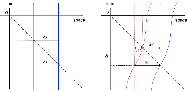
Figure 2: Spacetime diagram for two neighbouring galaxies (red and blue) as they cross the lightcone. In the left panel the galaxies are at rest with respect to the observer, while in the right panel they are moving away from the observer. The lightcone effect is that the density of crossings depends on the frame of observation, which will generally be boosted relative to the rest frame of the galaxies. Note that the total number of galaxies observed is equal to the number of worldlines crossing the past lightcone and is of course conserved in all frames.

III.2 Lightcone effect

In addition to the lookback time, there is also the so-called lightcone effect [41, 28]. This arises from the use of light as a means to probe the positions of galaxies, leading to a subtle correction to the number density if the galaxies are in motion (which they typically are). More precisely, when we measure the distance between two galaxies, what we do in practice is to measure the distance between two photons received at the same time by the observer. If the two galaxies are at different distances from the observer, the two photons were clearly not emitted at the same time. This leads to change in their observed separation if the galaxies are not at rest with respect to the observer. The overall correction is very similar to but distinct from the Doppler shift (the wave-like properties of light not needed).

The effect can be seen by considering the separation between two neighbouring galaxies along the same line of sight, as in Figure 2. The effect arises because the separation $\delta x^{\prime}$ inferred from light received and the ideal separation $\delta x$ measured at fixed time do not coincide if galaxies are observed in motion. (Conversely, there is no effect if the galaxy pair is at rest with respect to the observer, $\delta x^{\prime}=\delta x$.) This means that the number density of galaxies reckoned by the observer according to their lightcone is not necessarily the same as the number density on a surface of fixed time, which is what is typically assumed. The effect is a consequence of the travel time of light between objects (along the line of sight) and is present even if one could measure the real-space positions of galaxies.

The relation between $\delta x$ and $\delta x^{\prime}$ can be found by considering the time it takes for a photon emitted by the blue galaxy to reach the red galaxy (see Figure 2). If the galaxies are at rest with respect to the observer then the distance travelled is $\delta x$. However, if the galaxies are moving away from the observer with velocity $v>0$, the red galaxy moves towards the photon (in the observer frame), so that the photon does not have to cover the full distance $\delta x$ (as depicted in the right panel of Figure 2). In the time $\delta t$ it takes for the photon from the blue galaxy to reach the red galaxy the red galaxy covers a distance $v\hskip 0.59998pt\delta t$, meaning that the photon only has to travel a distance $\delta x^{\prime}=\delta x-v\hskip 0.59998pt\delta t$. Since the travel time of the photon between the blue and red galaxies is $\delta t=\delta x^{\prime}/c$, the inferred separation is therefore

$$\delta x^{\prime}=\delta x/(1+v/c)\,.$$ (19)

This is also the separation seen by the observer, since once the photon emitted by the blue galaxy has reached the red galaxy, the two photons travel together at the same speed and reach the observer at the same time.

In the primed coordinates the observer then measures a number density $\mathrm{d}N/\mathrm{d}x^{\prime}=(1+v/c)\,\mathrm{d}N/\mathrm{d}x$, that is, the observer sees the density $\mathrm{d}N/\mathrm{d}x$ either enhanced or suppressed, depending on the state of motion of galaxies (at the time of photon emission). In three dimensions this becomes

$$n(\mathbf{x})\to\tilde{n}(\mathbf{x})\equiv n(\mathbf{x})\hskip 0.59998pt[1+\mathbf{v}(\mathbf{x})/c\cdot\hat{\mathbf{x}}]\,,$$ (20)

where $\tilde{n}(\mathbf{x})$ is the apparent number density and, as before, $n(\mathbf{x})=\bar{n}[1+\delta(\mathbf{x})]$ is the underlying number density. Note that this is a line-of-sight effect so only the radial density is affected. This leads to a front-back asymmetry just as we have with the gravitational redshift. For instance, on the near side of an overdense patch, where galaxies are infalling away from us, the number density is biased high, whereas on the far side, where they are streaming towards us, it is biased low. For typical speeds, $v\simeq 300\,\mathrm{km\,s}^{-1}$, the bias (or asymmetry) is at the $0.1\%$ level, small but not negligible in the context of gravitational redshift.

As emphasized by Kaiser [41], the lightcone effect is not specific to cosmology but can be seen in a variety of contexts. Take for instance a photograph of a particle cloud, where at any given instant of time there are on average as many particles moving away from us as towards us [41]. According to the lightcone effect, the photograph—which captures each particle at slightly different times and not at fixed time—will show more particles moving away from us than towards us (which is not to say that the velocities can be inferred from the photograph itself). A useful way to understand this is by following the photons, arriving (simultaneously) from a given line of sight, back down the lightcone. We can imagine replacing the received photons by a single messenger travelling backwards in time from the observer, passing through the particles on the lightcone without stopping. From this perspective, the messenger will overtake more particles moving towards them than moving away from them—in exactly the same way that a trail runner will encounter more hikers coming towards them than going away from them.

III.2.1 Covariant formulation

The lightcone effect, along with all other relativistic effects, can of course be obtained systematically from a covariant treatment of the number counts of galaxies [63, 64, 65, 66]. Here we will not repeat the full calculation but simply point out the origin of the lightcone effect in the calculation. We will hence focus only on the relevant kinematic part needed to see the effect, ignoring gravitational effects, e.g. the metric perturbations which lead to order $(\mathcal{H}/k)^{2}$ corrections in the number counts. In this section we thus assume a metric with line element $\mathrm{d}s^{2}=g_{\mu\nu}\mathrm{d}x^{\mu}\mathrm{d}x^{\nu}=a^{2}(\tau)(-\mathrm{d}\tau^{2}+\mathrm{d}\mathbf{x}^{2})$.

In the relativistic context, both the galaxy number density and the volume element are frame-dependent quantities. Therefore to obtain a covariant expression of number conservation it is preferable to work with the covariant galaxy four-current $J^{\hskip 0.49164pt\mu}=n_{\mathrm{p}}\hskip 0.59998ptu^{\mu}$, where $u^{\mu}$ is the galaxy four-velocity and $n_{\mathrm{p}}(x)$ is the physical number density, as would be measured in the rest frame of the galaxies. The volume element on an arbitrary three-surface is given by [69]

$$\mathrm{d}\Sigma_{\mu}=\frac{1}{3!}\sqrt{-g}\,\varepsilon_{\mu\nu\rho\lambda}\,\mathrm{d}x^{\nu}\wedge\mathrm{d}x^{\rho}\wedge\mathrm{d}x^{\lambda}\,,$$ (21)

where $g$ is the metric determinant and $\varepsilon_{\mu\nu\rho\lambda}$ is the Levi-Civita symbol. Note that $\mathrm{d}\Sigma_{\mu}$ is a vector of three-forms whose direction is specified by the four-vector normal to $\mathrm{d}\Sigma_{\mu}$ (or, more accurately, the one-forms dual to the three-forms). The usual Euclidean volume element corresponds to that of a three-surface of constant time: $\mathrm{d}\Sigma_{\mu}=\delta_{\mu 0}\sqrt{-g}\hskip 0.89996pt\mathrm{d}^{3}\mathbf{x}$, with $\mathrm{d}^{3}\mathbf{x}=\frac{1}{3!}\hskip 0.59998pt\varepsilon_{ijk}\,\mathrm{d}x^{i}\wedge\mathrm{d}x^{j}\wedge\mathrm{d}x^{k}=\mathrm{d}x^{1}\wedge\mathrm{d}x^{2}\wedge\mathrm{d}x^{3}$.

The differential number of galaxies $\mathrm{d}N$ is the flux of the galaxy four-current $J^{\mu}$ across three-surface $\mathrm{d}\Sigma_{\mu}$:

$$\mathrm{d}N={J}^{\hskip 0.49164pt\mu}\hskip 0.59998pt\mathrm{d}\Sigma_{\mu}=\frac{1}{3!}\sqrt{-g}\,n_{\mathrm{p}}\hskip 0.59998ptu^{\mu}\hskip 0.59998pt\varepsilon_{\mu\nu\rho\lambda}\,\mathrm{d}x^{\nu}\wedge\mathrm{d}x^{\rho}\wedge\mathrm{d}x^{\lambda}\,.$$ (22)

The total number of galaxies on the surface $\Sigma$ is given by the flux integral $\int_{\Sigma}{J}^{\hskip 0.49164pt\mu}\hskip 0.59998pt\mathrm{d}\Sigma_{\mu}$. To recover the conventional expression $\mathrm{d}N=n(x)\hskip 0.89996pt\mathrm{d}^{3}\mathbf{x}$, take a three-surface of constant time, $\mathrm{d}\Sigma_{\mu}=\delta_{\mu 0}\sqrt{-g}\hskip 0.89996pt\mathrm{d}^{3}\mathbf{x}$. Then $\mathrm{d}N=n_{\mathrm{p}}(x)\hskip 0.59998ptu^{\mu}\hskip 0.59998pt\delta_{\mu 0}\sqrt{-g}\hskip 0.59998pt\mathrm{d}^{3}\mathbf{x}=a^{3}n_{\mathrm{p}}(x)\hskip 0.59998pt\mathrm{d}^{3}\mathbf{x}=n(x)\hskip 0.59998pt\mathrm{d}^{3}\mathbf{x}$, where $a^{3}n_{\mathrm{p}}(x)=n(x)$ is the comoving number density and we used that $u^{0}=a^{-1}$. But as emphasised in the previous section, galaxies are counted on a surface of constant time for the observer, which differs from the surface of constant time for the galaxies, if the galaxies are moving with respect to us. Since we cannot perform local measurements, the number counts are obtained remotely from light received, and we thus define $\mathrm{d}\Sigma_{\mu}$ with respect to our past lightcone, such that the null vector $k^{\mu}\propto(1,-\hat{\mathbf{x}})$ is normal to the surface $\mathrm{d}\Sigma_{\mu}$. In other words, the ‘volume element’ $\mathrm{d}\Sigma_{\mu}$, in which we observe galaxies, lives on a lightlike three-surface, not a spacelike one.

Now to show that there is a lightcone effect of the form given by Eq. (20) it is enough to consider a galaxy living on the $z$-axis at $x\equiv(\tau,\mathbf{x})=(\tau_{0}-\chi^{\prime},0,0,\chi^{\prime})$ and moving purely along the $z$-axis at a non-relativistic speed, $u^{\mu}=a^{-1}(1,0,0,v)$ in the observer’s frame. The null vector is $k^{\mu}\propto(1,0,0,-1)$ and the nonzero entries of $\mathrm{d}\Sigma_{\mu}$ are $\mathrm{d}\Sigma_{0}=\mathrm{d}x^{1}\mathrm{d}x^{2}\mathrm{d}x^{3}$ and $\mathrm{d}\Sigma_{3}=-\mathrm{d}\tau\hskip 0.59998pt\mathrm{d}x^{1}\mathrm{d}x^{2}$. The observed number of galaxies $\mathrm{d}N=J^{\mu}\mathrm{d}\Sigma_{\mu}$ about the point $x$ on the lightcone is then

$$\mathrm{d}N =n_{\mathrm{p}}(x)\,a^{-1}\sqrt{-g}\hskip 0.59998pt\big{(}\mathrm{d}x^{1}\mathrm{d}x^{2}\mathrm{d}x^{3}-v\,\mathrm{d}\tau\hskip 0.59998pt\mathrm{d}x^{1}\mathrm{d}x^{2}\big{)}$$

$$=n(x)\hskip 0.59998pt(1+v)\hskip 0.89996pt\mathrm{d}^{3}\mathbf{x}\,,$$

where the second line is obtained by using that on the past lightcone $\mathrm{d}\tau=-\mathrm{d}x^{3}$. If we now generalise to a galaxy observed in arbitrary direction $\hat{\mathbf{x}}$ with velocity $\mathbf{v}=\mathbf{v}(x)$, we will instead have $\mathrm{d}N=n(x)(1+\mathbf{v}\cdot\hat{\mathbf{x}})\hskip 0.89996pt\mathrm{d}^{3}\mathbf{x}$, thus recovering Eq. (20).

Compared with the analysis of the previous section, here $1+\mathbf{v}\cdot\hat{\mathbf{x}}$ emerges as the tilt between the galaxy’s worldline (with tangent $J^{\mu}$) and the lightcone (with tangent $k^{\mu}$) at the point of intersection $x$. The $+\mathbf{v}\cdot\hat{\mathbf{x}}$ is because both light and galaxies are moving with respect to the observer. If one or both are at rest with respect to the observer there is no effect. (Note that it is not simply the tilt between the surface of constant time on which the galaxies are living and the surface of constant time at the observer; rather it is the tilt between the surface of constant time on which the galaxies and the lightcone which is at the origin of the effect.) From this we understand that for the tilt to be non-unity, and so for there to be an effect at all, it is essential that neither the galaxies nor the messenger (the photons) are at rest in the observer’s frame. (Of course, the photons are never at rest.) Indeed, if we boost to a frame in which the galaxies at $x$ are at rest (so $u^{\mu}=a^{-1}{\delta^{\hskip 0.49164pt\mu}}_{0}$), there is no lightcone effect.

III.3 Complete expression of the number density

With the results of the preceding sections we can now give an expression for the redshift-space density, corrected for the lightcone and lookback time effects. Begin again from number conservation, which now reads $n^{(\mathrm{s})}_{A}(\mathbf{s})\hskip 0.59998pt\mathrm{d}^{3}\mathbf{s}=n_{A}(\mathbf{x})(1+\mathbf{v}\cdot\hat{\mathbf{n}})\hskip 0.89996pt\mathrm{d}^{3}\mathbf{x}$. By similar steps to the ones leading to Eq. (3), we obtain

$$\begin{split}n^{(\mathrm{s})}_{A}(\chi)&=\frac{1}{\chi^{2}}\int^{\infty}_{0}\chi^{\prime 2}\mathrm{d}\chi^{\prime}n_{A}(\chi^{\prime})[1+\mathbf{v}(\chi^{\prime})\cdot\hat{\mathbf{n}}]\\[-3.0pt] &\qquad\qquad\quad\times\,\delta_{\mathrm{D}}\big{[}\chi-\chi^{\prime}-\delta\chi(\chi^{\prime})\big{]}\,,\end{split}$$ (23)

where $\delta\chi$ is given by Eq. (2), as before, and we used the shorthand $n_{A}^{(\mathrm{s})}(\chi)=n_{A}^{(\mathrm{s})}(\tau_{0}-\chi,\chi\hat{\mathbf{n}})$, $n_{A}(\chi^{\prime})=n_{A}(\tau_{0}-\chi^{\prime},\chi^{\prime}\hat{\mathbf{n}})$, etc. The integration here is along the line of sight, in time and space (similar to the lensing convergence integral). Of course Eq. (23) can be expressed in terms of the overdensity $\delta^{(\mathrm{s})}_{A}(\chi)$, using $n^{(\mathrm{s})}_{A}(\chi)=\bar{n}^{(\mathrm{s})}_{A}[1+\delta^{(\mathrm{s})}_{A}(\chi)]$.

Equation (23) provides a compact way of accounting for all relevant effects affecting the number density of galaxies. In this expression, wide-angle effects result from the radial measure $\chi^{2}\mathrm{d}\chi$ (number of sources per radial bin varies with distance for a given solid angle); fluctuations in the redshift due to large-scale structure enter through the map in the delta function; and as we have discussed in the previous section, the fact that light is used to probe the positions of tracers yields a velocity correction to the underlying density (a kind of kinematic selection effect).

III.3.1 Recovering linear perturbation theory

It is not difficult to show that the well-known linear expression (1) for the overdensity is contained within Eq. (23). Linearizing Eq. (23) by expanding the delta function to first order in $\delta\chi$ (see Ref. [60], section 4, for details), and using that

$$\frac{\mathrm{d}}{\mathrm{d}\chi}\hskip 0.59998ptf(\tau_{0}-\chi,\chi\hat{\mathbf{n}})=\left(\frac{\partial}{\partial\chi}-\frac{\partial}{\partial\tau}\right)f(\tau,\chi\hat{\mathbf{n}})\,,$$ (24)

we obtain at leading order the compact formula

$$\delta_{A}^{(\mathrm{s})} =\tilde{\delta}_{A}+\frac{1}{\chi^{2}}\left(\frac{\partial}{\partial\tau}-\frac{\partial}{\partial\chi}\right)\left(\chi^{2}\frac{1}{\mathcal{H}}(\mathbf{v}\cdot\hat{\mathbf{n}}-\Psi+\Psi_{O})\right)\,,$$ (25)

where $\mathcal{H}=\mathcal{H}(\tau)$, $\mathbf{v}=\mathbf{v}(\tau,\chi\hat{\mathbf{n}})$, $\Psi=\Psi(\tau,\chi\hat{\mathbf{n}})$, etc, and $\tilde{\delta}_{A}=b_{A}\delta+\mathbf{v}\cdot\hat{\mathbf{n}}$ is the lightcone-corrected overdensity (as observed in the absence of redshift fluctuations). Note that here we have reinstated the $1/\mathcal{H}(\tau)$ since it is also differentiated.

The form of Eq. (25) shows at once the structure underlying the various terms, signs, prefactors and derivatives in Eq. (1). In particular, the time derivative traces back to the lookback time where by expanding the full formula (23) we are in effect computing the Jacobian of the spacetime map (17).

Now, evaluating the derivatives in Eq. (25) we see that all terms in Eq. (1) are indeed recovered:

$$\delta_{A}^{(\mathrm{s})} =\delta_{A}+\mathbf{v}\cdot\hat{\mathbf{n}}-\frac{1}{\mathcal{H}}\frac{\partial}{\partial\chi}(\mathbf{v}\cdot\hat{\mathbf{n}}-\Psi)+\frac{1}{\mathcal{H}}(\dot{\mathbf{v}}\cdot\hat{\mathbf{n}}-\dot{\Psi})$$

$$\qquad\qquad-\left(\frac{2}{\mathcal{H}\chi}+\frac{\dot{\mathcal{H}}}{\mathcal{H}^{2}}\right)(\mathbf{v}\cdot\hat{\mathbf{n}}-\Psi+\Psi_{O})\,.$$ (26)

In fact, we have also recovered additional terms which do not appear Eq. (1) (but which are contained in the relativistic derivation [64, 65, 63, 66]) such as $\Psi$ and $\dot{\Psi}$; these are all of order $(\mathcal{H}/k)^{2}$, and so have been neglected in Eq. (1). We could have even gone further and accounted for other $(\mathcal{H}/k)^{2}$ terms. For example, it is straightforward to add the ISW contribution to the redshift displacement (2), which would lead to several extra terms in Eq. (26). The transverse Doppler effect (a second-order contribution to redshift) may also be included in a similar way.

That we are able to recover Eq. (1) in very few steps derives from the fact that the redshift perturbation, taking us from real space to redshift space, determines most of the terms in the full expression of $\delta^{(\mathrm{s})}$, as was pointed out in Ref. [46]. As we can see, the large number of terms is simply due to the product rule.

III.4 Complete model of the correlation function

The complete model for the redshift-space correlation function, including all $\mathcal{H}/k$ effects, follows from Eq. (23). The derivation is similar to the one before, the main difference now being that the underlying real-space statistics are slightly modified due to the lightcone effect. However, Eq. (20) indicates that this simply amounts to the following replacement throughout the model: $1+\delta_{A}(\mathbf{x}_{1})\to[1+\delta_{A}(\mathbf{x}_{1})][1+\mathbf{v}(\mathbf{x}_{1})\cdot\hat{\mathbf{n}}_{1}]$ and $1+\delta_{B}(\mathbf{x}_{2})\to[1+\delta_{B}(\mathbf{x}_{2})][1+\mathbf{v}(\mathbf{x}_{2})\cdot\hat{\mathbf{n}}_{2}]$. In particular, this leads to the following change in the normalisation of the density-weighted averages:

$$1+\xi_{AB}(r) \to\langle[1+\delta_{A}(\mathbf{x}_{1})][1+\mathbf{v}(\mathbf{x}_{1})\cdot\hat{\mathbf{n}}_{1}]$$

$$\qquad\times[1+\delta_{B}(\mathbf{x}_{2})][1+\mathbf{v}(\mathbf{x}_{2})\cdot\hat{\mathbf{n}}_{2}]\rangle$$ (27)

$$=\big{[}1+\xi_{AB}(r)\big{]}\big{[}1+\llangle v_{\|1}+v_{\|2}+v_{\|1}v_{\|2}\rrangle\big{]}\,.$$

Thus the underlying real-space correlation function is kinematically ‘modulated’. This means that even before accounting for RSD we will observe stronger clustering in regions where the galaxy pair is streaming away from us than when they are streaming towards us.

Finally, by repeating the same steps that led to Eq. (4), and using that the underlying correlation function is replaced with Eq. (27), we have for the complete model

$$1+\xi^{(\mathrm{s})}_{AB}(\bm{\chi}) =\frac{1}{\chi_{1}^{2}\hskip 0.59998pt\chi_{2}^{2}}\int\mathrm{d}\chi_{1}^{\prime}\hskip 0.59998pt\chi_{1}^{\prime 2}\int\mathrm{d}\chi_{2}^{\prime}\hskip 0.89996pt\chi_{2}^{\prime 2}\,\big{[}1+\xi_{AB}(\bm{\chi}^{\prime})\big{]}$$

$$\qquad\times\big{[}1+\llangle v_{\|1}+v_{\|2}+v_{\|1}v_{\|2}\rrangle\big{]}\hskip 0.89996ptp(\bm{\chi}\,|\,\bm{\chi}^{\prime})\,,$$ (28)

where the time dependence in all quantities is now actively integrated over since there is a $\chi^{\prime}$ dependence in $\tau$, e.g. $v_{\|i}=\mathbf{v}(\tau_{0}-\chi^{\prime}_{i},\chi_{i}^{\prime}\hat{\mathbf{n}}_{i})\cdot\hat{\mathbf{n}}_{i}$. The form of this expression is essentially the same as Eq. (4) (had we absorbed the kinematic part into the definition of $\xi_{AB}$). However, the integration is now a line integral directed down the lightcone instead of on a fixed-time slice. Apart from the kinematic factor, there is one other difference when compared to the previous expression (9). This difference is found in the cumulants of $p$, which are now weighted by $\tilde{n}_{A}(\mathbf{x})=n_{A}(\mathbf{x})(1+\mathbf{v}\cdot\hat{\mathbf{x}})$ instead of $n_{A}(\mathbf{x})$. The form of $p$ is otherwise the same. Unless otherwise stated, double brackets $\llangle\cdots\rrangle$ will henceforth denote the following lightcone-corrected density-weighted average:

$$\llangle F(\mathbf{x}_{1},\mathbf{x}_{2})\rrangle =\frac{\langle\tilde{n}_{A}(\mathbf{x}_{1})\hskip 0.89996pt\tilde{n}_{B}(\mathbf{x}_{2})F(\mathbf{x}_{1},\mathbf{x}_{2})\rangle}{\langle\tilde{n}_{A}(\mathbf{x}_{1})\hskip 0.89996pt\tilde{n}_{B}(\mathbf{x}_{2})\rangle}\,,$$ (29)

replacing the previous one given by Eq. (8). (But note that the distinction between this average and the previous one is not particularly important for the level of approximation used in this work.)

IV Model inputs

Our focus up to now has been on the formal relation between correlations in redshift space and those in real space, independent of the specific biased tracer used or how the underlying fields might evolve gravitationally. We will henceforth specialise to dark matter haloes, as per the RayGalGroup catalogues (used in the model validation to follow).

Clearly a number of real-space correlation functions are needed in the model (28). These enter through the components of $\bm{m}$ and $\mathbf{C}$ of the Gaussian distribution function. Although these components consist of two-point functions, because of the density weighting they will generally also contain contributions from higher-order statistics, namely the (integrated) bispectrum and the (integrated) trispectrum. In this work we neglect such contributions and consider only contributions which are at most quadratic in fields. We thus approximate, e.g. $\llangle u_{\|}(\mathbf{x}_{1})\rrangle\simeq\langle u_{\|}(\mathbf{x}_{1})\hskip 0.59998pt\delta(\mathbf{x}_{2})\rangle[1+\xi_{AB}(r)]^{-1}$ and $\llangle u_{\|}(\mathbf{x}_{1})\hskip 0.59998ptu_{\|}(\mathbf{x}_{2})\rrangle\simeq\langle u_{\|}(\mathbf{x}_{1})u_{\|}(\mathbf{x}_{2})\rangle[1+\xi_{AB}(r)]^{-1}$ (where terms such as $\langle u_{\|}(\mathbf{x}_{1})\hskip 0.59998pt\delta(\mathbf{x}_{1})\hskip 0.59998pt\delta(\mathbf{x}_{2})\rangle$ have been neglected). As shown in Appendix B, with this approximation, $\bm{m}$ and $\mathbf{C}$ are composed of seven (scalar) correlation functions between $\delta$, $\mathbf{u}$, and $\psi$: $\xi_{\delta\delta}$, $\xi_{u\delta}$, $\xi_{\psi\delta}$, $\xi_{uu}^{\parallel}$, $\xi_{uu}^{\perp}$, $\xi_{u\psi}$ and $\xi_{\psi\psi}$. We evaluate these correlations at linear order in perturbation theory and assume linear bias. As we will see in Section V when comparing with numerical simulations, these approximations work well in the mildly nonlinear regime.

There is however one exception to this, which is the contribution from $\llangle\psi(\mathbf{x})-\psi_{O}\rrangle$ that enters $\bm{m}_{\mathrm{grav}}$ [Eq. (11)]. For this term, linear perturbation theory is not enough and a good estimate of this inherently nonlinear quantity is needed to reproduce simulation measurements of the dipole (see Section V). The reason is that $\llangle\psi(\mathbf{x})-\psi_{O}\rrangle$ contains the one-point function $\langle\psi(\mathbf{x})\hskip 0.59998pt\delta(\mathbf{x})\rangle$ (from the density weighting), which is sensitive to small-scale nonlinearities and to shot noise. In contrast, the analogous one-point function of RSD (entering $\bm{m}_{\mathrm{RSD}}$) vanishes due to parity, $\langle u_{\|}(\mathbf{x})\delta(\mathbf{x}))\rangle=0$. Hence $\langle\psi(\mathbf{x})\hskip 0.59998pt\delta(\mathbf{x}))\rangle$ is the only one-point function in $\bm{m}$ for which we need to go beyond linear theory. In practice this nonperturbative input can either be estimated given a prescription of the (highly) nonlinear regime, or it can be measured from numerical simulations, or else it can be treated as a free parameter, fitted together with cosmological parameters to data. In the following we compute $\llangle\psi(\mathbf{x})-\psi_{O}\rrangle$ using the halo model [70]. This gives at once the one-point function contained within.

IV.1 Density-weighted potential: nonlinear treatment

Since $\llangle\psi(\mathbf{x})-\psi_{O}\rrangle$ is a two-point correlation it decomposes in the usual way into a one- and two-halo term:

$$\llangle\psi(\mathbf{x})-\psi_{O}\rrangle=\llangle\psi(\mathbf{x})-\psi_{O}\rrangle_{\mathrm{1h}}+\llangle\psi(\mathbf{x})-\psi_{O}\rrangle_{\mathrm{2h}}\,.$$ (30)

The first term is the contribution from the internal halo structure (one-halo term) and the second term is the contribution from clustering as described by perturbation theory (two-halo term).

The important aspect of this statistic is the non-locality of the potential $\psi(\mathbf{x})$, because of which the one-halo term, nominally the shot noise contribution, yields a significant correction to the two-halo term at all separations. As we will see in Section VI, the one-point function $\langle\psi(\mathbf{x})\hskip 0.59998pt\delta(\mathbf{x})\rangle$ contained within is not well modelled using perturbation theory. The nature of density weighting skews the gravitational potential towards regions of high density (density contrast of several hundred) where tracers are likely to be found but where perturbation theory fails. In effect, the halo model augments the large-scale potential (described by perturbation theory) by the small-scale potential of the halo itself. The basic picture is of a smooth potential (sourced by large-scale structure) punctuated by sharp, local deviations due to dense dark matter haloes. Hence at the sites of tracers (the haloes), we find a large enhancement in the size of the one-point function. Since photons are emitted from the halos, they are affected by the small-scale potential. At linear order, this contribution vanishes, since the local potentials of two distant galaxies are uncorrelated and only the large-scale linear potential contributes to the correlation function. At nonlinear order, however, this is not the case any more and the signal is strongly boosted by this contribution.

To compute the one- and two-halo terms in Eq. (30) we first express the number density $n_{A}(\mathbf{x}_{1})$ and $n_{B}(\mathbf{x}_{2})$ (that enter through Eq. (8)) as a superposition of halos of mass $M_{A}$ and $M_{B}$ (or range of masses centred on $M_{A}$ and $M_{B}$). The gravitational potential $\psi(\mathbf{x})$ is sourced by haloes of all masses (according to some mass function), with each halo described by the same characteristic density profile. Details of the calculation are given in Appendix F; here we summarize the main results. For the one-halo terms we have

$$\begin{split}\!\!\llangle\psi(\mathbf{x}_{1})-\psi_{O}\rrangle_{\mathrm{1h}}&=[\phi_{A}(0)-\phi_{A}(\chi_{1}^{\prime})]-[\phi_{B}(\chi_{2}^{\prime})-\phi_{B}(r)]\,,\\ \!\!\llangle\psi(\mathbf{x}_{2})-\psi_{O}\rrangle_{\mathrm{1h}}&=[\phi_{B}(0)-\phi_{B}(\chi_{2}^{\prime})]-[\phi_{A}(\chi_{1}^{\prime})-\phi_{A}(r)]\,,\end{split}$$ (31)

where $\chi_{1}^{\prime}$ and $\chi_{2}^{\prime}$ are the comoving distance, in real space, to $\mathbf{x}_{1}$ and $\mathbf{x}_{2}$ and $r$ is the real-space separation between them. Here $\phi_{A}$ is the potential of an individual halo in population $A$; treated as an isolated body with spherically-symmetric density profile $\rho_{A}(r)$, the halo potential is given by

$$\phi_{A}(r)=\lambda\int^{\infty}_{r}\mathrm{d}r^{\prime}\hskip 0.59998pt\frac{GM_{A}(r^{\prime})}{r^{\prime 2}}\,,$$ (32)

with analogous expressions for tracer $B$. Here $\lambda\equiv\mathcal{H}^{-1}a^{2}$, $G$ is Newton’s constant of gravitation, and $M_{A}(r)=4\pi\int^{r}_{0}\rho_{A}(x)\hskip 0.59998ptx^{2}\mathrm{d}x$ is the mass profile, normalised so that $M_{A}(r)=M_{A}$ for $r>R_{\mathrm{vir}}$, with $R_{\mathrm{vir}}$ the virial radius. The tracer dependence is through parameters like the mass which characterise the density profile. Note that if $r>R_{\mathrm{vir}}$ we have $\phi_{A}(r)=\lambda\hskip 0.59998ptGM_{A}/r$, i.e. the details of the density profile are irrelevant and the potential is given as if it was sourced by a point particle of mass $M_{A}$.

The two-halo terms are (see again Appendix F for details)

$$\llangle\psi(\mathbf{x}_{1})-\psi_{O}\rrangle_{\mathrm{2h}} =\frac{[\xi^{\mathrm{HM}}_{\psi\delta_{A}}(0)-\xi^{\mathrm{HM}}_{\psi\delta_{A}}(\chi_{1}^{\prime})]-[\xi^{\mathrm{HM}}_{\psi\delta_{B}}(\chi_{2}^{\prime})-\xi^{\mathrm{HM}}_{\psi\delta_{B}}(r)]}{1+\xi_{AB}(\chi_{1}^{\prime},\chi_{2}^{\prime},\cos\vartheta)},$$ (33)

$$\llangle\psi(\mathbf{x}_{2})-\psi_{O}\rrangle_{\mathrm{2h}} =\frac{[\xi^{\mathrm{HM}}_{\psi\delta_{B}}(0)-\xi^{\mathrm{HM}}_{\psi\delta_{B}}(\chi_{2}^{\prime})]-[\xi^{\mathrm{HM}}_{\psi\delta_{A}}(\chi_{1}^{\prime})-\xi^{\mathrm{HM}}_{\psi\delta_{A}}(r)]}{1+\xi_{AB}(\chi_{1}^{\prime},\chi_{2}^{\prime},\cos\vartheta)},$$

where $\xi^{\mathrm{HM}}_{\psi\delta_{A}}(r)$, corresponding to $\langle\psi(\mathbf{x})\hskip 0.59998pt\delta_{A}(\mathbf{x}^{\prime})\rangle$, is given by

$$\xi^{\mathrm{HM}}_{\psi\delta_{A}}(r)=\int\mathrm{d}M\frac{\mathrm{d}n}{\mathrm{d}M}\int\mathrm{d}^{3}\mathbf{x}\,\xi_{hh}(\mathbf{r}-\mathbf{x},M_{A},M)\hskip 0.89996pt\phi_{M}(\mathbf{x})\,,$$ (34)

and likewise for $B$. Here $\mathrm{d}n/\mathrm{d}M$ is the halo mass function, $\xi_{hh}$ is the halo correlation function, and $\phi_{M}$ is the potential (32) of a halo of mass $M$ [with $\phi_{A}=\phi_{M_{A}}$ and $\phi_{B}=\phi_{M_{B}}$]. We assume $\xi_{hh}(\mathbf{r},M,M^{\prime})=b_{1}(M_{A})\hskip 0.59998ptb_{1}(M^{\prime})\hskip 0.59998pt\xi_{mm}(r)$ with $b_{1}(M)$ estimated using the peak–background split. For numerical work we use an NFW profile [71] (truncated at the virial radius $R_{\mathrm{vir}}$) and a Sheth–Tormen mass function [72].

As might be noticed, the normalisation $1+\xi_{AB}$ from the density weighting is present in the two-halo term but not in the one-halo term. As shown in Appendix F, the apparent dependence of $\llangle\psi(\mathbf{x})-\psi_{O}\rrangle_{\mathrm{1h}}$ on the normalisation drops out upon taking into account the third-order statistic $\langle\psi\delta\delta\rangle$ contained within (in addition to the second-order statistic $\langle\psi\delta\rangle$). This ought to be the case for the one-halo term, which should not depend on clustering statistics like $\xi_{AB}$.

In Section VI we will revisit these quantities and show that $\xi^{\mathrm{HM}}_{\psi\delta}(r)$ is given to a good approximation by linear theory for virtually all separations, with corrections being higher derivative (suppressed for $r\gtrsim R_{\mathrm{vir}}$). More importantly, we will see that the one-halo term represents a sizeable correction to linear theory.

V Numerical results

In this section we validate the model (28) against $N$-body simulations, focussing on the dipole moment.

V.1 Multipole decomposition

To extract the multipoles from the model we will first need to make a change of coordinates. In particular, we change from spherical coordinates $(\chi_{1},\chi_{2},\cos\vartheta)$, which we have used so far, to standard coordinates $(s,d,\mu)$, where $s$ is the separation, $d$ is some measure of the distance to the pair, and $\mu=\hat{\mathbf{s}}\cdot\hat{\mathbf{n}}$ is the angle of the pair with respect to the line of sight $\hat{\mathbf{n}}$. In the wide-angle regime the latter set of coordinates are not uniquely specified but depend on the choice of line of sight (with respect to which the multipoles are defined). In this work the line of sight is chosen according to the mid-point parametrisation; this is the most ‘symmetric’ choice in that it minimises the wide-angle effects [73]. Definitions and coordinate relations can be found in Appendix I. After making this change of coordinates, we obtain the multipoles of $\xi^{(\mathrm{s})}$ through numerical integration of the standard formula:

$$\xi_{\ell}(s,d)=\frac{2\ell+1}{2}\int^{1}_{-1}\mathrm{d}\mu\,\mathcal{L}_{\ell}(\mu)\,\xi^{(\mathrm{s})}(s,d,\mu)\,,$$ (35)

where $\mathcal{L}_{\ell}$ is the Legendre polynomial of degree $\ell$. Note that the multipoles $\xi_{\ell}$ depend on the separation $s$ and the distance $d$ to the pair.

On the practical matter of evaluating Eq. (35), some care is required at the upper and lower limits, $\mu=\pm 1$. At these points the lines of sight coincide ($\hat{\mathbf{n}}_{1}=\hat{\mathbf{n}}_{2}$) meaning that Eq. (9) is integrated through a configuration in which both galaxies ‘collide’ ($\mathbf{x}_{1}=\mathbf{x}_{2}$). As a result $\mathbf{C}$ is singular and we essentially have a single light of sight, or one less degree of freedom in our problem. These edge cases, and those where $\mu$ is close to but not quite equal to $\pm 1$, correspond to extremely flattened triangles in Figure 1, i.e. where wide-angle effects are negligible and one should revert to using the streaming model in the distant-observer limit given by

$$1+\xi^{(\mathrm{s})}(s_{\|},s_{\perp}) =\int^{\infty}_{-\infty}\mathrm{d}r_{\|}\,\big{[}1+\xi(r)\big{]}\frac{1}{\sqrt{2\pi}\hskip 0.89996pt\sigma_{12}(r_{\|},s_{\perp})}$$

$$\qquad\times\exp\left(-\frac{[s_{\|}-r_{\|}-m_{\|}(r_{\|},s_{\perp})]^{2}}{2\hskip 0.59998pt\sigma_{\|}^{2}(r_{\|},s_{\perp})}\right)\,,$$ (36)

where $r=(r_{\|}^{2}+r_{\perp}^{2})^{1/2}$, $r_{\|}$ is the (real-space) separation along the line of sight, and $r_{\perp}=s_{\perp}$ is the separation perpendicular to the line of sight. We also have the first and second moments, $m_{\|}(r_{\|},r_{\perp})=\llangle\Delta\chi\rrangle$ and $\sigma_{\|}^{2}(r_{\|},r_{\perp})=\llangle\Delta\chi^{2}\rrangle$, with $\Delta\chi\equiv\delta\chi(\mathbf{x}_{1})-\delta\chi(\mathbf{x}_{2})$ wherein $\hat{\mathbf{n}}_{1}=\hat{\mathbf{n}}_{2}$. (In the absence of gravitational redshift these are the familiar pairwise velocity moments.) As we have shown in Ref. [60] (see Appendix B), Eq. (36) is indeed a limiting case of the full wide-angle model (9).

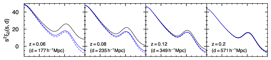
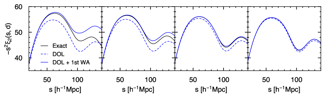
Figure 3: Comparison between the Gaussian streaming model in the exact wide-angle regime (solid black) and in the usual distant-observer limit (DOL; dashed blue). The solid blue curves show how close we can get to the exact result by simply adding the leading-order wide-angle correction to the DOL curve. Top row shows the monopole, bottom row the quadrupole. For this comparison we turn off all effects except RSD and associated wide-angle effects (no gravitational redshift, lightcone, etc). Here we have used the mid-point parametrisation, a Planck 2018 cosmology, and assumed no galaxy bias.

V.2 Impact of wide-angle effects on even multipoles

Before we turn to the complete model, let us first focus exclusively on the wide-angle aspect of the model, ignoring all effects except RSD (no gravitational redshift, lightcone effect, lookback time, etc). The results for the even multipoles are shown in Figure 3, illustrating the perturbativity of the wide-angle corrections as we go to higher redshift (or distance). As a basis of comparison we also show the standard Gaussian streaming model (in the distant-observer limit). As expected, we see large wide-angle corrections at large separations. For fixed distance $d$ (or redshift) these corrections grow with the opening angle $\vartheta$, and in the perturbative regime ($\vartheta\ll 1$) we use $\epsilon\equiv s/d\approx\vartheta$ as a small parameter to organize the wide-angle corrections. These large separations are within the linear regime and do not necessarily imply a need for a nonlinear dynamical treatment; linear dynamics is sufficient, although perhaps not near the BAO scale [74]. However, one can still have large wide-angle corrections at small separation if the distance $d$ is small, so that $\epsilon$ is large (see the lowest redshift bins).

To get a sense of how nonperturbative the departures are we also show an approximate model in which we simply add the leading-order wide-angle correction to the standard streaming model (36) (which at lowest order goes as $\epsilon^{2}$, not $\epsilon$, in the mid-point parametrisation. Comparing this model with the exact model (which contains wide-angle corrections at all orders in $\epsilon$), it is seen that both models converge by a redshift $z=0.2$, with quadrupole already well converged at $z=0.12$. Furthermore, the quadrupole at $z=0.08$ is also reasonably well accounted for by just the linear correction up to $s=100\,h^{-1}\mathrm{Mpc}$, while the monopole appears less so. This is because of the integration of the correlation function over $\mu$; some wedges are less susceptible to wide-angle effects than others, e.g. the ones aligned with the line of sight. The monopole gives equal weight to all wedges ($\mathcal{L}_{0}=1$), and in particular those where the galaxy pair is perpendicular to the line of sight ($\mu\simeq 0$); here the opening angle $s/d$ is largest (for fixed separation $s$) and thus large wide-angle corrections. By contrast the quadrupole gives about half weight, $\mathcal{L}_{2}(\mu)=(3\mu^{2}-1)/2\simeq-1/2$, to the same configurations and thus the quadrupole is driven more by wedges aligned with the line of sight, where as we mentioned we are less prone to wide-angle effects.

To determine the relevance of wide-angle effects, we compare them with the uncertainties on the measurements of the multipoles. For a survey like the DESI Bright Galaxy Sample, we find that wide-angle corrections for the monopole are of similar size as the 1$\sigma$ uncertainties in the lowest redshift bin ($z=0.15$), see Figure 10 in Appendix E. At redshift $z=0.25$, wide-angle corrections are still about half on the 1$\sigma$ uncertainties. Since the goal of surveys like DESI is to keep systematic effects at their minimum, such large biases should be avoided and wide-angle effects should properly be accounted for in the modelling.

V.3 Model validation

V.3.1 RayGalGroup simulation

For this comparison we use the publicly available halo catalogues from the RayGalGroup simulation, a dark-matter only $N$-body simulation of $4096^{3}$ particles in a box of size $(2625\,h^{-1}\mathrm{Mpc})^{3}$ [67, 75]. Haloes are identified using a pFoF halo-finding algorithm with linking length $b=0.2$ and a minimum particle count of 100. The particle mass-resolution is $1.88\times 10^{10}\,h^{-1}M_{\odot}$. The simulations were initialised from a power spectrum using a WMAP7 cosmology with $\Omega_{m}=0.25733$, $\Omega_{b}=0.04356$, $\Omega_{r}=8.076\times 10^{-5}$, $h=0.72$, $A_{s}=2.42\times 10^{-9}$, and $n_{s}=0.963$.

The catalogues are constructed from the $4\pi$ lightcone, with the observed position of the halo connected to its true position by ray tracing backwards from the observer to the source. The redshift and angular position, obtained by solving the null geodesic equations in the weak-field approximation, contain the total effect of Doppler shift (including the relativistic transverse part), gravitational redshift, gravitational lensing, time delay, and integrated Sachs–Wolfe. In the halo catalogues, each of these contributions to the total redshift have been separated. In our comparison, following Ref. [48], we keep only the contributions due to Doppler shift and gravitational redshift. The lightcone and lookback time effects are not included in this comparison. The redshift range is $z_{\mathrm{min}}=0.05$ to $z_{\mathrm{max}}=0.465$; the effective redshift is $z=0.341$, corresponding to a distance $d=950\,h^{-1}\mathrm{Mpc}$.

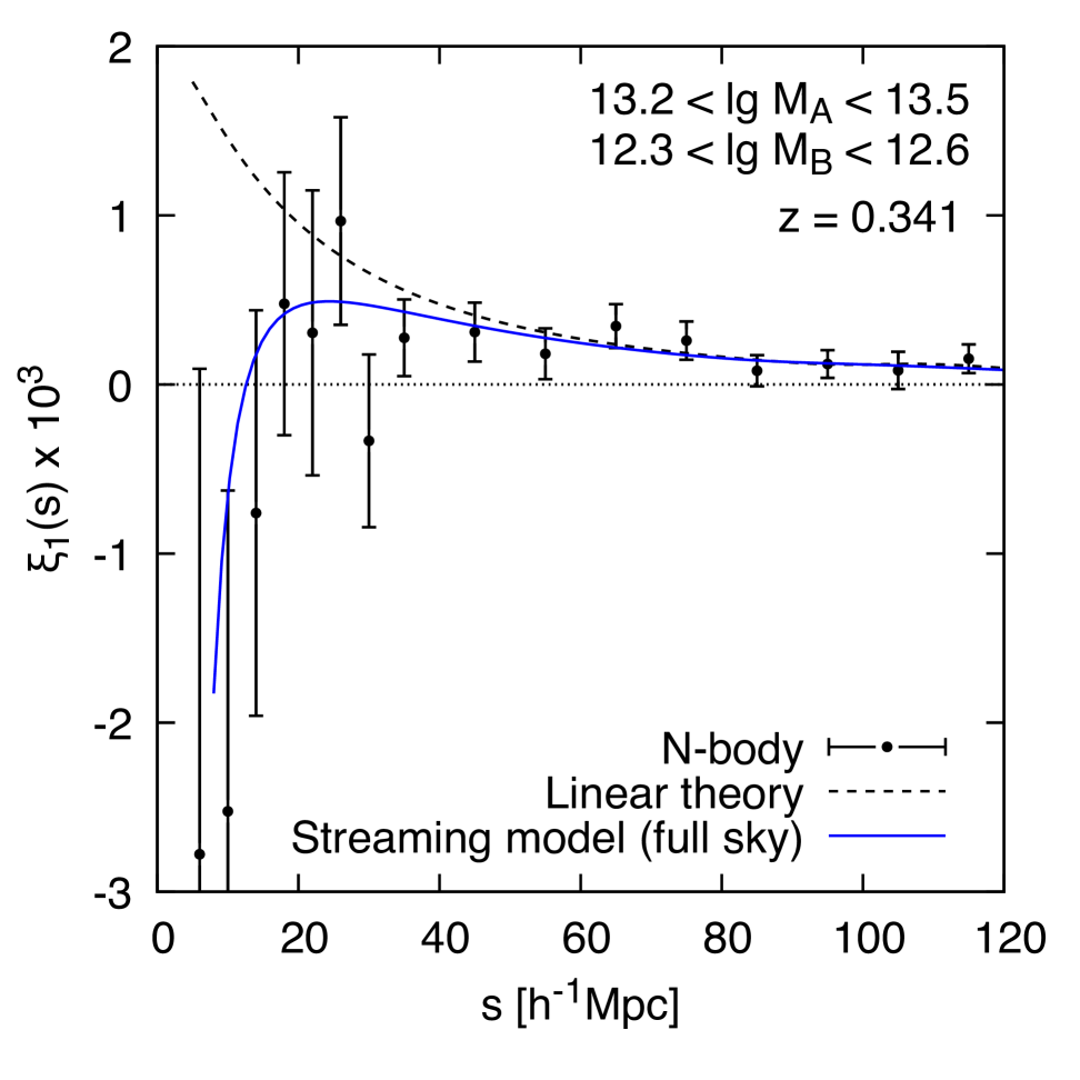
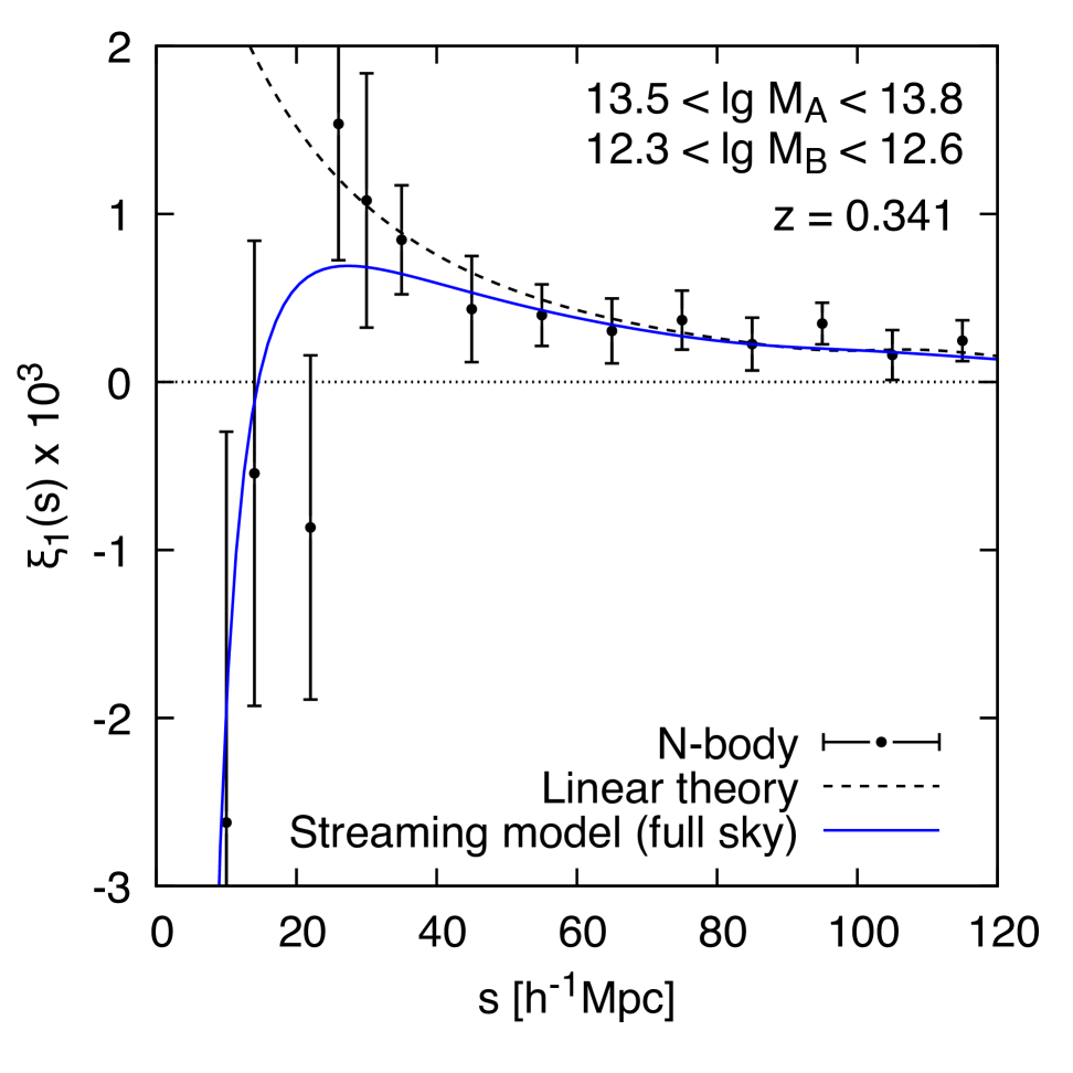
Figure 4: Comparison between model prediction (28) and dipole measurements from the RayGalGroup simulation. Left panel and right panel differ by choice of high-mass haloes: on the left we have mean mass $M_{A}=2.2\times 10^{13}\,h^{-1}M_{\odot}$, while on the right $M_{A}=4.5\times 10^{13}\,h^{-1}M_{\odot}$; in both $M_{B}=0.28\times 10^{13}\,h^{-1}M_{\odot}$. The model is evaluated using the mass ranges shown in the plot. The statistical uncertainty is estimated using the jack-knife method from 32 resamplings. Note that measurements at $s\leq 32\,h^{-1}\mathrm{Mpc}$ have a slightly finer binning than those at $s>32\,h^{-1}\mathrm{Mpc}$.

Table 2: Halo catalogues used in this work. Here $b_{1}$ is the estimated linear bias and $c$ the estimated mean halo concentration.

No. of haloes	No. of particles	Mean mass [$h^{-1}M_{\odot}$]	$b_{1}$	$c$
$5.4\times 10^{6}$	100–200	$0.28\times 10^{13}$	$1.08$	$8.2$
$1.0\times 10^{6}$	800–1600	$2.2\times 10^{13}$	$1.69$	$6.6$
$0.4\times 10^{6}$	1600–3200	$4.5\times 10^{13}$	$2.07$	$6.1$

The dipole is estimated from the cross-correlation of a high-mass bin with mean mass $2.2\times 10^{13}h^{-1}M_{\odot}$ (tracer $A$) and a low-mass bin with mean mass $0.28\times 10^{12}h^{-1}M_{\odot}$ (tracer $B$). We also consider a higher-mass bin with mean mass $4.5\times 10^{13}h^{-1}M_{\odot}$. See Table 2 for further details.

V.3.2 Dipole comparison

To compute the dipole, we evaluate the seven linear two-point correlation functions that enter into $\bm{m}$ and $\mathbf{C}$ (using the WMAP7 cosmology, as per the RayGal simulation). Moreover, we compute the nonlinear one-point correlation functions of Eq. (31) according to the specifications of the halo catalogue. The linear galaxy bias is calculated from the peak–background split using a Sheth–Tormen mass function [72], which is integrated over mass ranges given in Table 2. Specifically, tracer $A$ ranges from $M_{A1}=10^{13.2}h^{-1}M_{\odot}$ to $M_{A2}=10^{13.5}h^{-1}M_{\odot}$, while tracer $B$ ranges from $M_{B1}=10^{12.3}h^{-1}M_{\odot}$ to $M_{B2}=10^{12.6}h^{-1}M_{\odot}$. The formula for $\llangle\psi(\mathbf{x})-\psi_{O}\rrangle_{\mathrm{1h}}$, in the case of mass bins of finite width, has the same form as Eq. (31) but with the halo potentials replaced by their mass-weighted average:

$$\phi_{A}(\mathbf{x})\to\bar{\phi}_{A}(\mathbf{x})\equiv\frac{1}{\bar{n}_{A}}\int^{M_{A2}}_{M_{A1}}\mathrm{d}M\hskip 0.89996pt\frac{\mathrm{d}{n}}{\mathrm{d}M}\,\phi(\mathbf{x};M)\,,$$ (37)

where $\bar{n}_{A}=\int^{M_{A2}}_{M_{A1}}\mathrm{d}M\hskip 0.89996pt{\mathrm{d}n}/{\mathrm{d}M}$ is the mean density of population $A$ (and likewise for population $B$).

Figure 4 compares our theoretical model of the dipole with measurement from the RayGal catalogues, for different galaxy populations. At separations $s\lesssim 30\,h^{-1}\mathrm{Mpc}$ we see a clear departure of linear theory (which gives a positive dipole) from the measurements (which cross zero and become negative). Our model prediction on the other hand provides a better fit to the measurements. The point of zero crossing is also broadly consistent with the simulations in both panels. In the right panel we see however a slight enhancement in the amplitude of the dipole, which is not fully captured by our model. But the large uncertainty in the measurements, due to lower halo numbers, makes it difficult to draw any firm conclusions here. In Section VII we will discuss in detail the physical origin of the turnover. In brief, the turnover and eventual zero crossing is due to a cancellation in the effects of wide-angle RSD and gravitational redshift, marking a regime where the gravitational redshift begins to dominate over RSD and other kinematic effects.

Note that in order to reproduce the turnover it is essential that we have a realistic estimate of the one-point functions. These enter the density-weighted potential (30), by way of $\bm{m}_{\mathrm{grav}}$. As mentioned in Section IV.1, these one-point functions are estimated using the halo model, for which there is a contribution coming from the one-halo term and another from the two-halo term. For the population with mean mass $M_{A}=2.2\times 10^{13}h^{-1}M_{\odot}$ we find $\phi_{A}(0)=0.036\,h^{-1}\mathrm{Mpc}$, which represents a more than $100\%$ correction on top of the two-halo contribution $\xi_{\psi\delta_{A}}^{\mathrm{HM}}(0)=0.022\,h^{-1}\mathrm{Mpc}$. The linear estimate of the one-point function is virtually identical to the two-halo estimate (for reasons that will become clear in Section VI.3.3). By itself, the linear estimate is unable to reproduce the turnover and needs to be augmented by a small-scale contribution (e.g. the one-halo term).

Aside from these small-scale considerations, we have additionally performed a check on the importance of $\mathbf{C}_{\mathrm{cross}}$ and $\mathbf{C}_{\mathrm{grav}}$ on the dipole. We find almost identical results for the dipole with and without these contributions (i.e. keeping just $\mathbf{C}_{\mathrm{RSD}}$ in the covariance). This tells us that the important contributions to the dipole comes from the mean $\bm{m}$. We have also checked the impact $\mathbf{C}_{\mathrm{cross}}$ and $\mathbf{C}_{\mathrm{grav}}$ have on the monopole and quadrupole. For $s<150\,h^{-1}\mathrm{Mpc}$, we find these contributions also to be negligible (less than $0.1\%$ at $s=100\,h^{-1}\mathrm{Mpc}$, for example). This is of course not surprising given that in Fourier space one expects these contributions only to become important on scales approaching the horizon [47].

V.3.3 Impact of lightcone and lookback-time effects

To assess the impact of the lightcone and lookback time effects we investigate two versions of the streaming model: one with all the effects included (‘all’), as given by Eq. (28), and one where we exclude lightcone and lookback time effects, keeping all other effects (‘base’). (For the former model we use the lightcone-corrected density weighting (29), while for the latter we use Eq. (8).) The result is shown in Figure 5, in which we also show the linear predictions given by Eq. (1). Comparing the two streaming models we see that the lightcone and lookback time have a small net negative contribution to the dipole, consistent with findings elsewhere [67]. Although the amplitude is lowered slightly, the overall shape of the dipole remains largely the same. This rules out either of these effects as the cause of the turnover. (In Section VII below we will confirm this.)

An under-appreciated feature of the dipole (and all odd multipoles), is that it vanishes at zero separation, $\xi_{1}(s=0,d)=0$. This is because the overall contribution to the two-point correlation, $\xi_{1}(s,d)\hskip 0.59998pt\mathcal{L}_{\ell}(\mu)$, for odd $\ell$, is anti-symmetric about the axis $s_{\|}=0$ (the axis orthogonal to the line of sight) and is therefore required to vanish along this axis. We see this clearly for the linear theory curves in Figure 5, which return to zero at $s=0$. In principle, this is also the case for the streaming model, where we expect a very late turnaround as $s\to 0$ (which we are unable to show due to numerical instabilities in the model at small scales). We thus expect a second turnover in the dipole on very small scales for the complete model, where by contrast linear theory gives only one. But an improved treatment of the nonlinear regime (taking into account the higher-order correlations, halo exclusion, etc) is needed for a quantitative prediction here.

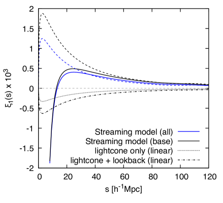
Figure 5: Dipole of the streaming model (solid blue) and from linear theory (dashed blue). For comparison we show in solid black the dipole from the streaming model without lightcone or lookback-time effects (the ‘base’ model), with the corresponding linear prediction shown in dashed black. The individual contribution from the lightcone effect given by linear theory is shown in dotted black; the sum of (linear) lightcone and lookback-time effects is shown in dash-dot black.

VI Anti-symmetries, parity, and pairwise functions

The way the displacement statistics of Section II.2 are currently written obscures the physical ingredients of the model. In this section we will bring out these ingredients by showing that these statistics naturally decompose into symmetric and anti-symmetric parts, with each part able to be reduced to a set of pairwise correlation functions (as in the distant-observer limit). The advantage of these pairwise functions is that they each have a distinct physical meaning, allowing us to isolate the important anti-symmetric effects (independent of the complications to do with the lines of sight).

VI.1 Decomposition of cumulants into symmetric and anti-symmetric parts

We consider two galaxies observed at $\mathbf{s}_{1}$ and $\mathbf{s}_{2}$, and label $A$ the galaxy at $\mathbf{s}_{1}$ and $B$ the galaxy at $\mathbf{s}_{2}$. (This label is generic and could describe galaxy bias, colour, luminosity, etc, although for concreteness we take this to be the galaxy bias.) In the distant-observer limit, and considering only the usual RSD effect we have that $\langle AB\rangle=\langle BA\rangle$; the order in which the two galaxies are paired does not matter. However, as shown in Ref. [28], when generalising beyond RSD and the distant-observer limit this is no longer the case. This motivates us to think of the labels $A$ and $B$ as an ordered pair given by the 2-tuple $(A,B)$. We can then determine which contributions to the two-point function are invariant under particle exchange, $(A,B)\to(B,A)$, and which contributions are not. Ultimately, the properties of $\langle\delta_{A}^{(\mathrm{s})}(\mathbf{s}_{1})\hskip 0.59998pt\delta_{B}^{(\mathrm{s})}(\mathbf{s}_{2})\rangle$ are determined by the cumulants $\bm{m},\mathbf{C},\ldots$, and by decomposing them into symmetric and anti-symmetric parts we can isolate in a systematic way only those terms which affect the odd multipoles.

For what follows, it will be convenient to restore labels $A$ and $B$, writing $\bm{m}\to\bm{m}_{AB}$ and $\mathbf{C}\to\mathbf{C}_{AB}$. With this notation we split each term into two parts:

$$\bm{m}_{AB}=\bm{m}_{(AB)}+\bm{m}_{[AB]}\,,\quad\mathbf{C}_{AB}=\mathbf{C}_{(AB)}+\mathbf{C}_{[AB]}\,,$$ (38)

where each part is given by

$$\bm{m}_{(AB)} =\tfrac{1}{2}(\bm{m}_{AB}+\bm{m}_{BA})\,, \quad\bm{m}_{[AB]} =\tfrac{1}{2}(\bm{m}_{AB}-\bm{m}_{BA})\,,$$

$$\mathbf{C}_{(AB)} =\tfrac{1}{2}(\mathbf{C}_{AB}+\mathbf{C}_{BA})\,, \quad\mathbf{C}_{[AB]} =\tfrac{1}{2}(\mathbf{C}_{AB}-\mathbf{C}_{BA})\,.$$

Under exchange $A\leftrightarrow B$, the first parts are symmetric ($\bm{m}_{(BA)}=\bm{m}_{(AB)}$) while the second parts are anti-symmetric ($\bm{m}_{[BA]}=-\bm{m}_{[AB]}$). Each of these quantities receive contributions from RSD and gravitational redshift and we write, for instance, $\bm{m}_{[AB]}=\bm{m}_{[AB]}^{\mathrm{RSD}}+\bm{m}_{[AB]}^{\mathrm{grav}}$.

VI.2 Pairwise correlations

We now apply decomposition (38) to each term in $\bm{m}=\bm{m}^{\mathrm{RSD}}+\bm{m}^{\mathrm{grav}}$ [Eq. (11)]. To avoid inessential complications and introducing too many novelties at once, we will present the following decomposition without the lightcone effect, i.e. we assume a symmetric density weighting, as in Eq. (8). In Section VI.2.2 we will discuss why this is justified.

Using that $\langle\psi(\mathbf{x}_{1})\hskip 0.59998pt\delta_{A}(\mathbf{x}_{2})\rangle=\langle\psi(\mathbf{x}_{2})\hskip 0.59998pt\delta_{A}(\mathbf{x}_{1})\rangle$ and $\langle\mathbf{u}(\mathbf{x}_{2})\hskip 0.59998pt\delta_{A}(\mathbf{x}_{1})\rangle=-\langle\mathbf{u}(\mathbf{x}_{1})\hskip 0.59998pt\delta_{A}(\mathbf{x}_{2})\rangle$, and likewise for $B$, we find that each term decomposes as

$$\bm{m}^{\mathrm{RSD}}_{AB} =\bm{m}^{\mathrm{RSD}}_{(AB)}+\bm{m}^{\mathrm{RSD}}_{[AB]}=\underbrace{\begin{pmatrix}\phantom{-}\tfrac{1}{2}\llangle\Delta\mathbf{u}\rrangle\cdot\hat{\mathbf{n}}_{1}\,\\[2.0pt] -\tfrac{1}{2}\llangle\Delta\mathbf{u}\rrangle\cdot\hat{\mathbf{n}}_{2}\end{pmatrix}}_{\text{sym.}}+\underbrace{\begin{pmatrix}\llangle\bar{\mathbf{u}}\rrangle\cdot\hat{\mathbf{n}}_{1}\\[2.0pt] \llangle\bar{\mathbf{u}}\rrangle\cdot\hat{\mathbf{n}}_{2}\end{pmatrix}}_{\text{anti-sym.}}\,,$$

$$\bm{m}^{\mathrm{grav}}_{AB} =\bm{m}^{\mathrm{grav}}_{(AB)}+\bm{m}^{\mathrm{grav}}_{[AB]}=\underbrace{\begin{pmatrix}\llangle\bar{\psi}\rrangle\\[2.0pt] \llangle\bar{\psi}\rrangle\end{pmatrix}}_{\text{sym.}}+\underbrace{\begin{pmatrix}\phantom{-}\tfrac{1}{2}\llangle\Delta\psi\rrangle\,\\[2.0pt] -\tfrac{1}{2}\llangle\Delta\psi\rrangle\,\end{pmatrix}}_{\text{anti-sym.}}\,,$$ (39)

where the symmetric and anti-symmetric parts are defined respectively by the first and second terms in the second equality. Here we have expressed $\mathbf{u}(\mathbf{x}_{1})$ and $\mathbf{u}(\mathbf{x}_{2})$, and similarly $\psi(\mathbf{x}_{1})-\psi_{O}$ and $\psi(\mathbf{x}_{2})-\psi_{O}$, in terms of new variables:

$$\Delta\mathbf{u} =\mathbf{u}(\mathbf{x}_{1})-\mathbf{u}(\mathbf{x}_{2})\,,\quad\;\,\bar{\mathbf{u}}=\tfrac{1}{2}[\mathbf{u}(\mathbf{x}_{1})+\mathbf{u}(\mathbf{x}_{2})]\,,$$ (40)

$$\Delta\psi =\psi(\mathbf{x}_{1})-\psi(\mathbf{x}_{2})\,,\quad\;\bar{\psi}=\tfrac{1}{2}[\psi(\mathbf{x}_{1})-\psi_{O}+\psi(\mathbf{x}_{2})-\psi_{O}]\,,$$

so that, e.g. $\mathbf{u}(\mathbf{x}_{1})=\bar{\mathbf{u}}+\Delta\mathbf{u}/2$. Note that all quantities in the right-hand side of Eq. (39) depend on the tracers $A$ and $B$ through the density weighting, even though here to simplify the notation we have dropped the subscript $AB$. Hence, e.g., the anti-symmetry of $\Delta\psi$ under the exchange of $\mathbf{x}_{1}$ and $\mathbf{x}_{2}$ results in an anti-symmetry of the weighted difference $\llangle\Delta\psi\rrangle_{AB}$ under the exchange of $AB$. This is easily verified by direct calculation:

$$\llangle\Delta\psi\rrangle_{BA} =(1+\xi_{AB})^{-1}\Big{[}\langle\psi(\mathbf{x}_{1})\hskip 0.59998pt\delta_{A}(\mathbf{x}_{2})\rangle-\langle\psi(\mathbf{x}_{2})\hskip 0.59998pt\delta_{B}(\mathbf{x}_{1})\rangle$$

$$\quad\qquad+\langle\psi(\mathbf{x}_{1})\hskip 0.59998pt\delta_{A}(\mathbf{x}_{1})\rangle-\langle\psi(\mathbf{x}_{2})\hskip 0.59998pt\delta_{B}(\mathbf{x}_{2})\rangle$$ (41)

$$\quad+\langle\psi(\mathbf{x}_{1})\hskip 0.59998pt\delta_{A}(\mathbf{x}_{1})\hskip 0.59998pt\delta_{B}(\mathbf{x}_{2})\rangle-\langle\psi(\mathbf{x}_{2})\hskip 0.59998pt\delta_{A}(\mathbf{x}_{2})\hskip 0.59998pt\delta_{B}(\mathbf{x}_{1})\rangle\Big{]}\,,$$

where each line is anti-symmetric under exchange of $A$ and $B$, so $\llangle\Delta\psi\rrangle_{BA}=-\llangle\Delta\psi\rrangle_{AB}$.

The basis (40) has the nice property that it is statistically independent: $\llangle\bar{\mathbf{u}}\Delta\mathbf{u}\rrangle=\llangle\Delta\mathbf{u}\bar{\mathbf{u}}\rrangle=0$ and $\llangle\bar{\psi}\Delta\psi\rrangle=\llangle\Delta\psi\bar{\psi}\rrangle=0$. In terms of the covariances, this is just the basis that diagonalizes $\mathbf{C}_{\mathrm{RSD}}$ and $\mathbf{C}_{\mathrm{grav}}$ (with the linear transformations containing all the line-of-sight dependence). The four quantities in Eq. (40) have a distinct physical meaning and their density-weighted averages, when reduced to their scalar parts, provide the basic objects of study (independent of geometrical factors from the lines of sight). To obtain the scalar parts of the velocity correlations, we recall that under statistical isotropy $\llangle\Delta\mathbf{u}\rrangle=\llangle\Delta u\rrangle\hat{\mathbf{r}}$ or $\llangle\Delta u\rrangle=\hat{\mathbf{r}}\cdot\llangle\Delta\mathbf{u}\rrangle$. Here $\llangle\Delta u\rrangle$ is (in our notation) the well-known pairwise velocity difference [56, 58], describing the tendency of infall of galaxy pairs as function of separation. Similarly, we also have a scalar correlation $\llangle\bar{u}\rrangle=\hat{\mathbf{r}}\cdot\llangle\bar{\mathbf{u}}\rrangle$, which we call the pairwise mean velocity (in the frame of the observer).

The symmetric pairwise correlation functions are thus

• $\llangle\Delta u\rrangle(r)\equiv\hat{\mathbf{r}}\cdot\llangle\Delta\mathbf{u}\rrangle$, the pairwise velocity difference;

• $\llangle\bar{\psi}\rrangle$, the pairwise mean potential;

while the anti-symmetric pairwise functions are

• $\llangle\bar{u}\rrangle(r)\equiv\hat{\mathbf{r}}\cdot\llangle\bar{\mathbf{u}}\rrangle$, the pairwise mean velocity;

• $\llangle\Delta\psi\rrangle(r)$, the pairwise potential difference.

Note that $\llangle\Delta u\rrangle$ and $\llangle\Delta\psi\rrangle$ are not of the same parity; the former is symmetric while the latter is anti-symmetric. As expected, the anti-symmetric functions are identically zero if $A=B$.

The parity of these pairwise functions determines whether they contribute at first order to the odd or even multipoles. Specifically, the symmetric pairwise functions contribute to the even multipoles, while the anti-symmetric ones contribute to the odd multipoles. (Note that at nonlinear order we can have products of these functions contributing to the multipoles, e.g. the product of a symmetric and anti-symmetric function, which is overall anti-symmetric.) Based on these properties we can already say that the important pairwise functions contributing to the dipole are $\llangle\bar{u}\rrangle$ and $\llangle\Delta\psi\rrangle$.

Another useful way to characterise these pairwise functions is by whether they are relative or absolute quantities. This property tells us in which regime the function enters and therefore whether it is a wide-angle effect, and if so at what order in $\epsilon=s/d$ it will contribute to the multipoles. To see this, recall that in the distant-observer limit we have only relative quantities appearing, $\llangle\Delta u\rrangle$, $\llangle\Delta\psi\rrangle$, etc. These generally depend purely on separation $r$ and are therefore the only types allowed by translation invariance (which exists in this limit but not in the wide-angle regime). The appearance in the wide-angle regime of ‘absolute’ quantities, $\llangle\bar{u}\rrangle$ and $\llangle\bar{\psi}\rrangle$, breaks translation invariance. For example, $\llangle\bar{\psi}\rrangle$ introduces dependence on the distances $\chi_{1}$ and $\chi_{2}$ between the galaxies and the observer (meaning we cannot translate the galaxy pair without fundamentally changing the triangle in Figure 1 on which the wide-angle correlations depend). This means that the wide-angle corrections of RSD and gravitational redshift are given in terms of the ‘absolute’ functions $\llangle\bar{u}\rrangle$ and $\llangle\bar{\psi}\rrangle$, respectively, and must enter the multipoles at order $\epsilon=s/d$ (vanishing in the distant-observer limit when $d\to\infty$). From these arguments, we can have a term of the form $\epsilon\hskip 0.59998pt\mathrm{d}\llangle\bar{u}\rrangle/\mathrm{d}s$ entering the dipole but not $\epsilon\hskip 0.59998pt\mathrm{d}\llangle\bar{\psi}\rrangle/\mathrm{d}s$ (where the derivative is required on dimensional grounds).

VI.2.1 Anti-symmetry of the lightcone effect

As another illustration, let us apply the decomposition to the kinematic factor in Eq. (28) to show that the lightcone effect induces an anti-symmetry at leading order. We have

$$\llangle u_{\|1}+u_{\|2}+u_{\|1}u_{\|2}\rrangle \simeq\llangle u_{\|1}+u_{\|2}\rrangle$$

$$=\llangle\mathbf{u}(\mathbf{x}_{1})\rrangle\cdot\hat{\mathbf{n}}_{1}+\llangle\mathbf{u}(\mathbf{x}_{2})\rrangle\cdot\hat{\mathbf{n}}_{2}$$

$$=\tfrac{1}{2}\hskip 0.59998pt\llangle\Delta u\rrangle\hskip 0.59998pt(\hat{\mathbf{r}}\cdot\hat{\mathbf{n}}_{1}-\hat{\mathbf{r}}\cdot\hat{\mathbf{n}}_{2})$$

$$\quad\;+\llangle\bar{u}\rrangle\hskip 0.59998pt(\hat{\mathbf{r}}\cdot\hat{\mathbf{n}}_{1}+\hat{\mathbf{r}}\cdot\hat{\mathbf{n}}_{2})\,,$$ (42)

where we have divided through by $\mathcal{H}$ and dropped the subdominant quadratic term (which at any rate is symmetric at leading order so not important for the odd multipoles). In the case $\hat{\mathbf{n}}_{1}=\hat{\mathbf{n}}_{2}$ (distant-observer limit) we see that only the second term in Eq. (42) remains, $\llangle\bar{u}\rrangle\propto(b_{A}-b_{B})\langle u\hskip 0.59998pt\delta\rangle$. This means that the impact of the lightcone effect at leading order is anti-symmetric and is present even in the distant-observer limit (unlike the anti-symmetric contribution from RSD).

Though we can also apply the decomposition to $\mathbf{C}_{AB}$ and obtain its pairwise ‘dispersion’ functions, it will not be necessary. As we found numerically in Section V, the impact of the covariance on the dipole is highly suppressed. Indeed, evaluated using linear theory, $\mathbf{C}_{AB}$ has no anti-symmetric part, $\mathbf{C}_{AB}=\mathbf{C}_{(AB)}$, since any anti-symmetric part can only come from the density weighting, which for $\mathbf{C}_{AB}$ enters at lowest order as a bispectrum contribution (which we ignore). In the remainder of this work, we will hence focus only on $\bm{m}_{AB}$ and its pairwise functions.

VI.2.2 Discussion

The decomposition into symmetric and anti-symmetric pairwise functions underlies the usual way of thinking about parity in terms of the number of radial derivatives carried by a given term in Eq. (1). When correlating with a single tracer (identical particles) there can be no anti-symmetry due to invariance under pair exchange. When correlating with distinct tracers (labelled particles) we have the possibility of anti-symmetry. Typically these parity properties are identified in the linear correlation function by looking at the number of radial derivatives a given term carries with respect to $\langle\delta\delta\rangle$. Those with an even (odd) number of derivatives will contain an even (odd) number of $\mu$’s and therefore contribute to the even (odd) multipoles, with the dependence on linear bias entering as $b_{A}+b_{B}$ ($b_{A}-b_{B}$). We can now see that this originates from the parity of the pairwise functions: for symmetric functions $\llangle\Delta u\rrangle$ and $\llangle\bar{\psi}\rrangle$ the biases enter as $b_{A}+b_{B}$, while for anti-symmetric functions $\llangle\Delta\psi\rrangle$ and $\llangle\bar{u}\rrangle$ the bias enters as $b_{A}-b_{B}$.

Although the parity is easy to see in linear theory, as above, it should be understood that the parity of these quantities holds at all orders in perturbation theory. So although we only consider linear bias in this work ($\delta_{A}\simeq b_{A}\hskip 0.59998pt\delta$ and $\delta_{B}\simeq b_{B}\hskip 0.59998pt\delta$), the above separation into terms proportional to bias sums ($b_{A}+b_{B}$) or bias differences ($b_{A}-b_{B}$) carries to higher-order galaxy bias. For instance, at second order there is nonlocal tidal bias and this also enters in the form $b_{K^{2}A}+b_{K^{2}B}$ or $b_{K^{2}A}-b_{K^{2}B}$. That this remains true is simply a consequence of the requirement that the galaxy bias expansion respect the equivalence principle, i.e. that galaxies symmetrically cluster with respect to the underlying matter.

As mentioned earlier, there is one complication and it is the effect of the lightcone correction on the pairwise functions. As we discussed, this changes the density weighting and in effect modifies the galaxy bias expansion through introduction of odd parity operators. This complicates the above analysis because we implicitly assumed that the bias expansion consists solely of even parity operators (a symmetric density weighting). As a result, we can no longer say that $\llangle\Delta\psi\rrangle$, with the lightcone-corrected density weighting (29), is totally anti-symmetric; it can also contain a symmetric part due to the additional factors of $1+\mathbf{v}\cdot\hat{\mathbf{n}}$. But this only leads to additional correlations in the form of $\langle\psi\hskip 0.59998ptv\rangle$ which is nominally suppressed relative to the other correlations $\langle\psi\hskip 0.59998pt\delta\rangle$ (and which is of the opposite parity anyway). There are also corrections in the form of a third-order statistic $\langle\psi\hskip 0.59998ptv^{2}\rangle$ which does affect the anti-symmetric part. But such terms are suppressed relative to $\langle\psi\hskip 0.59998pt\delta\rangle$. Altogether, this means that at leading order $\llangle\Delta\psi\rrangle$ remains unchanged and provided we work at this order we can continue to regard it as anti-symmetric. We note that similar considerations apply to the other pairwise functions.

VI.3 The pairwise potential difference

The numerical results and arguments above indicate that the key quantity governing the small-scale behaviour of the dipole is the pairwise potential difference $\llangle\Delta\psi\rrangle$. As Eq. (41) shows, this quantity contains contributions from the two-point correlation function, but also from the three-point functions that cannot be neglected.

VI.3.1 Linear contribution

As a first step, we study the behaviour of $\llangle\Delta\psi\rrangle$ at linear order, and then later in Sections VI.3.2 and VI.3.3 we compute the nonlinear corrections.

From the first two lines of Eq. (41), we have at linear order

$$\llangle\Delta\psi\rrangle =\frac{\big{[}{\xi_{\psi\delta_{A}}(0)-\xi_{\psi\delta_{A}}(r)}\big{]}-\big{[}{\xi_{\psi\delta_{B}}(0)-\hskip 0.59998pt\xi_{\psi\delta_{B}}(r)}\big{]}}{1+\xi_{AB}(r)}\,,$$ (43)

with $\xi_{\psi\delta_{A}}(r)=\langle\psi(\mathbf{x}_{1})\hskip 0.59998pt\delta_{A}(\mathbf{x}_{2})\rangle$ and $\xi_{\psi\delta_{B}}(r)=\langle\psi(\mathbf{x}_{1})\hskip 0.59998pt\delta_{B}(\mathbf{x}_{2})\rangle$. Writing $\xi_{\psi\delta_{A}}(r)=b_{A}\hskip 0.59998pt\xi_{\psi\delta}(r)$ and $\xi_{\psi\delta_{B}}(r)=b_{B}\hskip 0.59998pt\xi_{\psi\delta}(r)$, with $b_{A}$, $b_{B}$ the linear galaxy biases, and $\xi_{\psi\delta}(r)$ given by Eq. (86) in Appendix B, and using that at large separation, $\xi_{AB}(r)\ll 1$, we have

$$\llangle\Delta\psi\rrangle\simeq(b_{A}-b_{B})\,\big{[}{\xi_{\psi\delta}(0)-\xi_{\psi\delta}(r)}\big{]}\,.$$ (44)

This expression, with the galaxy biases made explicit, makes clear that $\llangle\Delta\psi\rrangle$ is anti-symmetric under the exchange of $A$ and $B$ and vanishes when $A=B$, as discussed above.

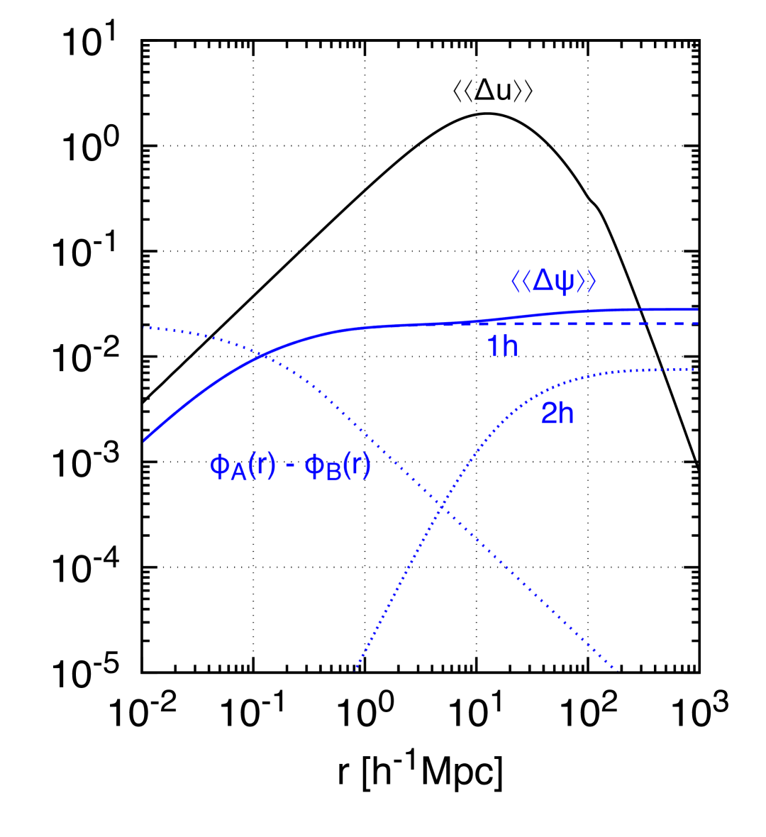
Figure 6: The contributions to the pairwise potential difference $\llangle\Delta\psi\rrangle=\llangle\Delta\psi\rrangle_{\mathrm{1h}}+\llangle\Delta\psi\rrangle_{\mathrm{2h}}$ (solid blue), where $\llangle\Delta\psi\rrangle_{\mathrm{1h}}$ is given by Eq. (46) and $\llangle\Delta\psi\rrangle_{\mathrm{2h}}$ is given by Eq. (34). For comparison, we also show the pairwise velocity difference $\llangle\Delta u\rrangle$ (which is negative valued). The scale dependent part of the one-halo term, $\phi_{A}(r)-\phi_{B}(r)$ is also shown. Note that in linear theory the $\llangle\bar{u}\rrangle$ differs from $\llangle\Delta{u}\rrangle$ by an order unity proportionality constant, $\llangle\bar{u}\rrangle=(b_{A}-b_{B})/(b_{A}+b_{B})\llangle\Delta u\rrangle$. All pairwise functions go to zero at $r=0$ and have units $h^{-1}\mathrm{Mpc}$. Here $b_{A}=2$, $b_{B}=1$, with $z=0.341$.

The key aspect of $\llangle\Delta\psi\rrangle$, setting it apart from $\llangle\Delta u\rrangle$, is that it does not vanish in the large-scale limit; see Figure 6. This is due to the presence of the one-point function, $\xi_{\psi\delta}(0)$, which is nonzero because modes $\psi(\mathbf{k})$ are in phase with $\delta(\mathbf{k})$ (or have the same parity). In the large-scale limit $\llangle\Delta\psi\rrangle\to(b_{A}-b_{B})\,\xi_{\psi\delta}(0)\neq 0$ as $r\to\infty$. Therefore, even at large separations $\llangle\Delta\psi\rrangle$ is sensitive to nonlinearities through $\xi_{\psi\delta}(0)$. By contrast the corresponding one-point function of $\llangle\Delta u\rrangle$ vanishes, since there are no preferred directions. So $\llangle\Delta u\rrangle$ goes to zero in the large-scale limit, with the tendency of pair infall decreasing with separation.

What is the impact of $\llangle\Delta\psi\rrangle$ on the redshift-space correlations $\xi^{(\mathrm{s})}$? Though the relation between $\xi^{(\mathrm{s})}$ and the pairwise functions is nonlocal, on dimensional grounds and recalling that $\Delta\psi$ has units length, we see that at linear order it is the derivative of $\llangle\Delta\psi\rrangle(r)$ with respect to $r$ that contributes to $\xi^{(\mathrm{s})}$. Consequently, at this order $\xi_{\psi\delta}(0)$ does not contribute to $\xi^{(\mathrm{s})}$. So although $\llangle\Delta\psi\rrangle$ appears to dominate over $\llangle\Delta u\rrangle$ at large $r$, its contribution is suppressed because of the flatness of $\llangle\Delta\psi\rrangle$ on these scales. The effect of the one-point function $\xi_{\psi\delta}(0)$ is however still relevant, since it enters at second order in $\xi^{(\mathrm{s})}$, and leads to a sizeable correction on small scales. We will show this explicitly in Section VII.2.

VI.3.2 Beyond linear theory: halo model approach

An improved estimate of $\llangle\Delta\psi\rrangle$, and in particular of the one-point function contained within, is obtained using the halo model. Again, since we have compared our model against halo catalogues, let us identify tracers $A$ and $B$ with two populations of dark matter haloes, described by mass $M_{A}$ and $M_{B}$ (among other parameters).

We split $\llangle\Delta\psi\rrangle$ into two contributions, writing

$$\llangle\Delta\psi\rrangle=\llangle\Delta\psi\rrangle_{\mathrm{1h}}+\llangle\Delta\psi\rrangle_{\mathrm{2h}}\,.$$ (45)

By taking the difference of $\llangle\psi(\mathbf{x}_{1})-\psi_{O}\rrangle/2$ and $\llangle\psi(\mathbf{x}_{2})-\psi_{O}\rrangle/2$, using the formulae of Section IV.1, it is easy to show that we have for the one- and two-halo terms

$$\llangle\Delta\psi\rrangle_{\mathrm{1h}} =[\phi_{A}(0)-\phi_{A}(r)]-[\phi_{B}(0)-\phi_{B}(r)]\,,$$ (46)

$$\llangle\Delta\psi\rrangle_{\mathrm{2h}} =\frac{[\xi^{\mathrm{HM}}_{\psi\delta_{A}}(0)-\xi^{\mathrm{HM}}_{\psi\delta_{A}}(r)]-[\xi^{\mathrm{HM}}_{\psi\delta_{B}}(0)-\xi^{\mathrm{HM}}_{\psi\delta_{B}}(r)]}{1+\xi_{AB}(r)}\,,$$ (47)

where we recall $\phi_{A}$ and $\phi_{B}$ are given by Eq. (32), and $\xi^{\mathrm{HM}}_{\psi\delta_{A}}$ and $\xi^{\mathrm{HM}}_{\psi\delta_{B}}$ are given by Eq. (34). Note that the local terms have cancelled out as expected so that both one- and two-halo terms are functions of $r$ only.

Let us note that the discreteness of the density field plays a crucial role in Eq. (46). Indeed, in the case where $\delta_{A}$ is a continuous field, related to the matter density through $\delta_{A}=b_{A}\delta$, the contribution from the three-point function to $\llangle\Delta\psi\rrangle$ vanishes due to symmetry. The third line in Eq. (41) becomes

$$b_{A}b_{B}\big{[}\langle\psi(\mathbf{x}_{1})\hskip 0.59998pt\delta(\mathbf{x}_{1})\hskip 0.59998pt\delta(\mathbf{x}_{2})\rangle-\langle\psi(\mathbf{x}_{2})\hskip 0.59998pt\delta(\mathbf{x}_{2})\hskip 0.59998pt\delta(\mathbf{x}_{1})\rangle\big{]}=0\,.$$ (48)

However, as we show in Appendix F, taking into account the discreteness of the density field, this third line does not vanish and leads to a non-negligible contribution to $\llangle\Delta\psi\rrangle$. This is due to the fact that when correlating $\delta_{A}(\mathbf{x}_{1})$ with $\psi(\mathbf{x}_{1})$ (that is sourced by all masses, as we see from Eq. (107)), the only contribution that survives is the one due to the potential $\phi_{A}$. And similarly $\delta_{B}(\mathbf{x}_{2})$ correlated with $\phi(\mathbf{x}_{2})$ gives rise to a contribution proportional to $\phi_{B}$. For $B\neq A$ this leads to a nonzero contribution from the three-point function in Eq. (41), which enters in the one-halo term $\llangle\Delta\psi\rrangle_{\mathrm{1h}}$. Physically, this term encodes the correlation between the density of the halo and the gravitational potential at the same position. Since this correlation differs for tracers $A$ and $B$, $\phi_{A}\neq\phi_{B}$, it contributes to the anti-symmetric part.

As Figure 6 shows, the one-halo term (46) dominates over the two-halo term at all scales $r$. Moreover, the individual contributions from $\phi_{A}(r)$ and $\phi_{B}(r)$ are negligible on scales $r\gg 1$ (beyond a few virial radii of the halo). On the other hand, $\phi_{A}(0)$ and $\phi_{B}(0)$ is relevant at all $r$ in that it sets an absolute scale on the depth of the halo potentials. Since these ‘one-point functions’ contain no scale dependence they shift $\llangle\Delta\psi\rrangle$ up and down; the same is also true for the corresponding $\xi^{\mathrm{HM}}_{\psi\delta_{A}}(0)$ and $\xi^{\mathrm{HM}}_{\psi\delta_{B}}(0)$, although they lead to smaller shifts. In Table 3 we compare the two contributions at zero separation for different halo masses. We see that, except for the lowest mass, the one-halo term dominates over the two-halo term by a factor of $1.5-6$. Note that all of these zero separation terms are degenerate with each other, however. The slight scale dependence seen in Figure 6 at $r\gtrsim 10\,h^{-1}\mathrm{Mpc}$ mainly enters through $\xi^{\mathrm{HM}}_{\psi\delta_{A}}(r)$ and $\xi^{\mathrm{HM}}_{\psi\delta_{B}}(r)$.

It is perhaps not surprising that the one-halo term is dominant: the density weighting biases the effect of gravitational redshift towards regions of high number density (galaxy clusters, dark matter haloes, etc), environments where high mass concentrations drive potential wells deeper than expectations from linear theory alone.

Table 3: Comparison between the one- and two-halo value of the potential depth, $\phi_{A}(0)$ and $\xi_{\psi\delta_{A}}(0)$, respectively. (To get a sense of the size relative to RSD, we have multiplied both quantities by $-\mathcal{H}$; the units are thus km/s.) The values are computed at $z=0.2$ using the Planck 2018 best-fit cosmology and assuming an NFW profile with concentration $c=9$ and truncated at the virial radius.

$M\hskip 0.89996pt[h^{-1}M_{\odot}]$	$R_{\mathrm{vir}}\,[h^{-1}\mathrm{Mpc}]$	$b_{1}$	$\xi_{\psi\delta_{A}}(0)\,[\text{km/s}]$	$\phi_{A}(0)\,[\text{km/s}]$
$10^{12}$	$0.18$	$0.87$	$-0.62$	$-0.32$
$10^{13}$	$0.39$	$1.39$	$-0.99$	$-1.48$
$10^{14}$	$0.84$	$2.80$	$-2.00$	$-6.89$
$10^{15}$	$1.80$	$7.68$	$-5.47$	$-31.96$

VI.3.3 Beyond linear theory: model-independent approach

Rather than resorting to a specific model of the halo profile, we will now pursue a more model-independent approach. In this section (and the next), we will show that the results of the previous section VI.3.2—in particular that there is negligible contribution to $\llangle\Delta\psi\rrangle$ from $\phi_{A}(r)$ and $\phi_{B}(r)$ for practically all $r$—holds under more general conditions than was assumed using the halo model.

We are interested in the gravitational potential outside the halo, treated here as an isolated, spherical but otherwise arbitrary body $\rho_{A}(\mathbf{x})$ with compact nonzero support on $|\mathbf{x}|<R_{\mathrm{vir}}$. (The assumption of spherical symmetry is not a strong one as we will shortly see.) In general the halo potential is given by

$$\phi_{A}(\mathbf{x})=\lambda G\int\mathrm{d}^{3}\mathbf{y}\,\frac{\rho_{A}(\mathbf{y})}{|\mathbf{x}-\mathbf{y}|}\,.$$ (49)

Expanding the Green’s function $1/|\mathbf{x}-\mathbf{y}|$ in the case $|\mathbf{x}|>|\mathbf{y}|$ (i.e. outside the halo when $|\mathbf{x}|>R_{\mathrm{vir}}$), we have the following well-known result from electrostatics:

$$\frac{1}{|\mathbf{x}-\mathbf{y}|}=\frac{1}{|\mathbf{x}|}-y_{i}\hskip 0.59998pt\partial_{i}\frac{1}{|\mathbf{x}|}+\frac{1}{2}y_{i}y_{j}\hskip 0.59998pt\partial_{i}\hskip 0.59998pt\partial_{j}\frac{1}{|\mathbf{x}|}+\cdots\,,$$ (50)

where $\partial_{i}=\partial/\partial x^{i}$. Substituting this expansion back into Eq. (49) and integrating over $\mathbf{y}$ we have, for $|\mathbf{x}|>R_{\mathrm{vir}}$,

$$\phi_{A}(\mathbf{x}) =\lambda\hskip 0.59998ptG\left({M}_{A}-M_{A}^{i}\hskip 0.59998pt\partial_{i}+\frac{1}{2}M_{A}^{ij}\hskip 0.89996pt\partial_{i}\hskip 0.59998pt\partial_{j}+\cdots\right)\frac{1}{|\mathbf{x}|}\,.$$ (51)

Here $M_{A}=\int\rho_{A}(\mathbf{x})\hskip 0.59998pt\mathrm{d}^{3}\mathbf{x}$, $M_{A}^{i}=\int x^{i}\rho_{A}(\mathbf{x})\hskip 0.59998pt\mathrm{d}^{3}\mathbf{x}$, $M_{A}^{ij}=\int x^{i}x^{j}\rho_{A}(\mathbf{x})\hskip 0.59998pt\mathrm{d}^{3}\mathbf{x}$, etc, are the mass moments of $\rho_{A}(\mathbf{x})$—numbers which completely characterize a given halo’s mass distribution. In general, the mass moments will differ from halo to halo (there need not be a universal profile).

Since we are dealing with a spherical mass distribution, all but the first term in Eq. (51) vanishes. This implies that the potential at $|\mathbf{x}|>R_{\mathrm{vir}}$ is given as if it was sourced by a point particle of mass $M$ and located at the body’s centre. This is known as Newton’s shell theorem and means that outside the halo the potential is completely determined by its mass with the usual inverse distance fall-off, $\phi\propto M/|\mathbf{x}|$; no knowledge of the body’s internal structure is required. (At least when dealing with the halo potential, we do not even need to make the usual halo-model assumption of a universal density profile.) In Eq. (46) the potentials are thus

$$\phi_{A}(r) =\lambda\hskip 0.59998pt\frac{GM_{A}}{r}\,,\quad r>R_{\mathrm{vir},A}\,,$$ (52a)

$$\phi_{B}(r) =\lambda\hskip 0.59998pt\frac{GM_{B}}{r}\,,\quad r>R_{\mathrm{vir},B}\,,$$ (52b)

where the only tracer-dependent parameter is the mass, $M_{A}$ and $M_{B}$. Since the largest collapsed objects have $R_{\mathrm{vir}}\simeq 2\,h^{-1}\mathrm{Mpc}$, which is still much smaller than typical separations $r$, these formulae are broadly applicable. Hence, for practically all separations $r$ we indeed satisfy the condition $r>R_{\mathrm{vir}}$.

These results have of course been obtained under the assumption that haloes are spherical. But even if we relax this assumption Eq. (52) remains a good approximation. Since although we would have nonvanishing higher moments, resulting in additional terms on the right-hand side of Eq. (52), these yield only small corrections to the basic picture above. On dimensional grounds, the $n$th moment is suppressed by a factor of order $(R_{\mathrm{vir}}/r)^{n}$ with respect to the leading contribution, $\phi\propto M/r$. In particular, if we make the weaker assumption that the halo is not spherical but symmetric so $\phi(-\mathbf{r})=\phi(\mathbf{r})$, then the leading correction comes from the quadrupole moment, which is suppressed by $(R_{\mathrm{vir}}/r)^{2}$.

Now, although we do not need a full description of the entire profile, we do require knowledge of the potential at $r=0$ (the depth), where the point-particle description clearly breaks down. In keeping with the model-independent approach, one way around this difficulty is to simply treat both $\phi_{A}(0)$ and $\phi_{B}(0)$ as free parameters (as is often done in data analysis with the Finger-of-God velocity dispersion parameter). In fact since these contributions are degenerate with those from Eq. (44), the total zero-point $\phi_{A}(0)+\xi_{\psi\delta_{A}}(0)-\phi_{B}(0)-\xi_{\psi\delta_{B}}(0)$ may be treated as a single unknown quantity.

Any symmetries (or lack thereof) in the profile carry over to $\llangle\Delta\psi\rrangle_{\text{1h}}$, which therefore depends in general on the (signed) quantity $\mathbf{r}=\mathbf{x}_{1}-\mathbf{x}_{2}$. Here we have assumed spherical symmetry. However, for an arbitrary profile Eq. (46) is exactly anti-symmetric under exchange $A\leftrightarrow B$ (or equivalently $\mathbf{x}_{1}\leftrightarrow\mathbf{x}_{2}$). But we do not strictly need to assume spherical symmetry for Eq. (46) to be anti-symmetric; we can still have have anti-symmetry in an approximate sense. On large scales haloes can be treated as effectively spherical point particles, regardless of their actual structure, since their aspherical moments are suppressed, see Eq. (53). At leading order the halo potential thus falls as $1/r$ so that for sufficiently large separations we can consider $\llangle\Delta\psi\rrangle_{\mathrm{1h}}$ as a function of $r$ only (and a weak function of $r$ at that). Whatever complicated structure haloes have when viewed on small scales is erased on sufficiently large scales, allowing us to view halos as effectively spherical with $\llangle\Delta\psi\rrangle_{\mathrm{1h}}$ as given by Eq. (46).

VI.3.4 Perturbation theory

We now show that the two-halo term (34) is largely insensitive to the particular details of the halo in that it differs only marginally from the linear predictions. This is of course a well known fact of the halo model. But in the case of the gravitational potential it is interesting to see why this is from the point of view of effective field theory.

The key observation is that on large scales a separation of scales emerges between $R_{\mathrm{vir}}$ and $r$. At larger and larger $r$ the detailed structure of the haloes themselves should be of diminishing importance in the large-scale description of clustering, so that to a first approximation one can treat haloes as point masses with $\rho(\mathbf{x})=M\delta_{\mathrm{D}}(\mathbf{x})$ and $\phi(\mathbf{x})\propto M/|\mathbf{x}|$. As is readily checked, the two-halo formula for $\xi_{\psi\delta_{A}}(r)$ [Eq. (34)] does indeed recover the linear expression (86) in the case of point masses and with linear galaxy bias, e.g. by writing the convolution in Eq. (34) in Fourier space and use that the Fourier transform of $1/4\pi|\mathbf{x}|$ is $1/k^{2}$.

If we now allow that haloes are of course extended objects, we can compute the corrections to the point-particle approximation. On dimensional grounds these corrections enter as terms going as the ratio of the size $R_{*}$ of the halo to the separation $r$. This is easy to see in Fourier space. Substituting an arbitrary density written in terms of its mass moments, $\rho(\mathbf{k})=M+\mathrm{i}k_{i}M_{i}-k_{i}k_{j}M_{ij}/2+\cdots$, into the potential $\phi(\mathbf{k})=4\pi G\lambda\hskip 0.89996pt\rho(\mathbf{k})/k^{2}$, we have [cf. Eq. (51)]

$$\phi(\mathbf{k})=\phi_{0}(\mathbf{k})\left(1+\mathrm{i}k_{i}M_{i}/M-\frac{1}{2}k_{i}k_{j}M_{ij}\hskip 0.59998pt/\hskip 0.59998ptM+\cdots\right)\,,$$ (53)

where $\phi_{0}(\mathbf{k})\equiv{4\pi\lambda\hskip 0.59998ptGM}/{k^{2}}$ is the potential of a point mass (here we omit tracer labels to ease notation). Thus the leading correction goes as $kR_{*}\sim R_{*}/r$ since $M_{i}\sim MR_{*}$. In the case of a spherical body the leading correction goes as $(kR_{*})^{2}\sim(R_{*}/r)^{2}$ since $M_{ij}\sim\delta_{ij}MR_{*}^{2}$.

These corrections carry over to the two-halo term (34). Writing Eq. (34) in Fourier form (and setting aside the unimportant galaxy bias), we find

$$\xi^{\mathrm{HM}}_{\psi\delta}(\mathbf{r}) =\int\frac{\mathrm{d}^{3}\mathbf{k}}{(2\pi)^{3}}\,\mathrm{e}^{-\mathrm{i}\mathbf{k}\cdot\mathbf{r}}P_{\delta\delta}(k)$$ (54)

$$\quad\times\lambda\frac{4\pi G\bar{\rho}}{k^{2}}\left(1+\mathrm{i}k_{i}A_{i}-\frac{1}{2}k_{i}k_{j}A_{ij}+\cdots\right)\,,$$

where $\bar{\rho}=\int\mathrm{d}M(\mathrm{d}n/\mathrm{d}M)M$ is the mean mass density and $A_{i},A_{ij}$, etc, are parameters characterising the spatial extent of haloes as a population average, i.e. integrated over the mass function. (By contrast $M,M_{i},M_{ij}$, etc, characterise only a particular halo in that population.) The usual expression of $\xi_{\psi\delta}(r)$ is recovered by dropping all but the first term in Eq. (54). From the perspective of effective field theory, $A_{i},A_{ij}$, etc, absorb the uncertain details of the mass function and profile (the two key ingredients of the halo model).

At the population level we can reasonably assume that haloes are on average spherical so that $A_{i}=0$ and $A_{ij}=\delta_{ij}\hskip 0.59998ptR_{*}^{2}$, with $R_{*}$ a free parameter corresponding to a characteristic spatial scale associated with the second mass moment. Inserting these back into Eq. (54) we find $\xi^{\mathrm{HM}}_{\psi\delta}(r)\simeq\big{(}1+R_{*}^{2}\nabla^{2}\big{)}\,\xi_{\psi\delta}(r)$, with $\xi_{\psi\delta}(r)$ given by the standard expression (86). The leading-order correction is thus a higher-derivative term and so is suppressed on large scales. In fact, for $r\gtrsim 2\,h^{-1}\mathrm{Mpc}$ we find very small differences numerically between $\xi_{\psi\delta}(r)$ and the halo model $\xi^{\mathrm{HM}}_{\psi\delta}(r)$ given by the full expression (34) (ignoring biasing complications). When evaluated using linear theory and assuming linear bias, we find that the two-halo term $\llangle\Delta\psi\rrangle_{\mathrm{2h}}$ is well approximated by the standard expression.

VII Origin of the dipole’s turnover

In this section we investigate the origin of the turnover in the dipole, as seen in Figure 5. As mentioned above, this turnover—which is absent in linear theory—is a direct signature of the nonlinear gravitational redshift signal. Using the results of Section VI and following the perturbative approach taken in the distant-observer limit [58]), we will analytically compute the dipole

$$\xi_{1}(s,d)=\frac{3}{2}\int^{1}_{-1}\mathrm{d}\mu\,\mathcal{L}_{1}(\mu)\,\xi^{(\mathrm{s})}_{AB}(s,d,\mu)$$ (55)

by performing an expansion of $\xi^{(\mathrm{s})}_{AB}$ [Eq. (9)], identifying the displacements $\delta\chi$ as the expansion parameter.

We will work to order $\epsilon\equiv s/d$ in the mid-point parametrisation and consider subleading contributions to Eq. (55) which are suppressed (in Fourier space) by a single power of $\mathcal{H}/k$ with respect to the matter power spectrum. We will thus ignore terms contributing to Eq. (55) at order $\epsilon^{2}$, $(\mathcal{H}/k)^{2}$ and $\epsilon\,\mathcal{H}/k$, all of which we will simply call terms $\mathcal{O}(\epsilon^{2})$.

VII.1 Small-displacement expansion

Typical displacements, which we did not require to be small in our derivation, tend to be small in practice. For instance, in $\Lambda$CDM $\delta\chi\simeq v/H_{0}\simeq 3\,h^{-1}\mathrm{Mpc}$, which is much smaller than the order $100\,h^{-1}\mathrm{Mpc}$ radial length scales ($\chi_{1}$ and $\chi_{2}$) associated with typical configurations. As our notation already suggests, we can thus think of the radial map (2) as slightly perturbing the sidelengths of the real-space triangle (Figure 1) while keeping the opening angle fixed. On this basis we can expand ‘real space around redshift space’ [58], in other words, we expand out the displacement in Eq. (4) then perform the resulting integrals analytically. Note that most of the support of $p$ is tightly centred around $\bm{m}$ (which turns out to be very close to the point at which $p$ attains its maximum value).

To facilitate the integration, we define the joint six-dimensional vectors $\bm{X}=(\mathbf{x}_{1},\mathbf{x}_{2})$, $\bm{S}=(\mathbf{s}_{1},\mathbf{s}_{2})$, and $\bm{\Delta}=\bm{S}-\bm{X}$. In these coordinates Eq. (4) takes the form

$$1+\xi_{AB}^{(\mathrm{s})}(\bm{S})=\int\mathrm{d}^{6}\bm{\Delta}\,\big{[}1+\xi_{AB}(\bm{S}-\bm{\Delta})\big{]}\,p(\bm{\Delta}\,|\,\bm{S}-\bm{\Delta})\,,$$ (56)

where the integration is now over the displacement $\bm{\Delta}$ and we have suppressed the dependence on $A$ and $B$. Since $\bm{\Delta}$ is small compared to $\bm{S}$ we expand $\xi_{AB}(\bm{S}-\bm{\Delta})$ and $p(\bm{\Delta}\,|\,\bm{S}-\bm{\Delta})$ around $\bm{S}$:

$$\xi_{AB}(\bm{S}-\bm{\Delta}) =\big{[}1-(\bm{\Delta}\cdot\bm{\partial})+\tfrac{1}{2}(\bm{\Delta}\cdot\bm{\partial})^{2}+\cdots\big{]}\,\xi_{AB}(\bm{S})\,,$$

$$p(\bm{\Delta}\,|\,\bm{S}-\bm{\Delta}) =\big{[}1-(\bm{\Delta}\cdot\bm{\partial})+\tfrac{1}{2}(\bm{\Delta}\cdot\bm{\partial})^{2}+\cdots\big{]}\hskip 0.59998ptp(\bm{\Delta}\,|\,\bm{S})\,,$$

where we have defined the joint partial derivative

$$\partial_{a}=\partial/\partial\hskip 0.59998ptS^{a}\,,\qquad a=1,2,\ldots,6\,$$ (57)

acting on six-dimensional Cartesian space. Substituting these back into Eq. (56) and using that

$$\textstyle\int\mathrm{d}^{6}\bm{\Delta}\hskip 0.59998ptp(\bm{\Delta}\,|\,\bm{S})\hskip 0.59998pt\Delta_{a} =m^{a}_{AB}\,,$$

$$\textstyle\int\mathrm{d}^{6}\bm{\Delta}\hskip 0.59998ptp(\bm{\Delta}\,|\,\bm{S})\hskip 0.59998pt\Delta_{a}\Delta_{b} =C^{ab}_{AB}+m^{a}_{AB}\hskip 0.59998ptm^{b}_{AB}\,,$$

where $\bm{m}_{AB}$ is now a 6-dimensional vector and $\mathbf{C}_{AB}$ a $6\times 6$ matrix, we find up to second order

$$\xi^{(\mathrm{s})}_{AB}=\xi_{AB}-\partial_{a}\hskip 0.59998ptm_{AB}^{a}+\tfrac{1}{2}\partial_{a}\partial_{b}C_{AB}^{ab}-m_{AB}^{a}\hskip 0.59998pt\partial_{a}\hskip 0.59998pt\xi_{AB}$$

$$\qquad+\tfrac{1}{2}\partial_{a}\partial_{b}\hskip 0.59998pt(m_{AB}^{a}\hskip 0.59998ptm_{AB}^{b})-\xi_{AB}\hskip 0.59998pt\partial_{a}\hskip 0.59998ptm_{AB}^{a}+\tfrac{1}{2}C_{AB}^{ab}\hskip 0.59998pt\partial_{a}\partial_{b}\hskip 0.59998pt\xi_{AB}$$

$$\qquad+\tfrac{1}{2}\xi_{AB}\hskip 0.89996pt\partial_{a}\hskip 0.59998pt\partial_{b}C_{AB}^{ab}+\partial_{a}\hskip 0.59998pt\xi_{AB}\hskip 0.59998pt\partial_{b}C_{AB}^{ab}+\mathcal{O}(\xi_{AB}^{3})\,.$$ (58)

Here repeated indices $a,b$ are summed over (no sum over $A,B$) and all terms on the right-hand side are real-space quantities evaluated at the redshift-space position, i.e. at $\bm{X}=\bm{S}=(\mathbf{s}_{1},\mathbf{s}_{2})$. The first three terms on the right-hand side contain the usual leading-order contributions while the rest of the terms are quadratic in correlations (induced by the nonlinear part of the redshift map). In the case of distortions due purely to RSD, we have previously shown [60] that the first three terms recovers the usual Kaiser multipoles along with the leading-order wide-angle corrections.

The type of terms appearing in Eq. (58) is revealing. Although we know from the nonperturbative expression of $\xi^{(\mathrm{s})}_{AB}$ [Eq. (9)] that the dependence on the underlying real-space correlations is nonlocal, the expansion (58) shows that beyond linear order (where $m^{a}$ or $C_{ab}$ only appear in differentiated form) we also have terms with local dependence on $m^{a}$ and $C_{ab}$ (e.g. $m_{AB}^{a}\hskip 0.59998pt\partial_{a}\hskip 0.59998pt\xi_{AB}$). This has a key consequence for the dipole because $m^{a}$ (and $C_{ab}$) contains one-point functions (‘dispersions’) whose effect on $\xi^{(\mathrm{s})}_{AB}$ is not necessarily differentiated away at second order. In other words, the absolute scale of $m^{a}$ is important.

VII.2 Perturbative expression of the dipole

To capture the turnover occurring on small to intermediate scales, we now compute the dipole of $\xi^{(\mathrm{s})}_{AB}$ using the expansion (58), keeping terms up to second order in correlations. Although there are a large number of terms, fortunately not all of them contribute to the dipole and we can discard many of them. In particular, since $\mathbf{C}_{AB}=\mathbf{C}_{(AB)}$ the linear term $\partial_{a}\partial_{b}C^{ab}_{AB}$ does not contribute to the odd multipoles and can be ignored.

To further simplify the calculation we will neglect the lightcone and lookback-time effects. As we saw in Figure 5, the turnover is present in the absence of these effects (the full second-order expression including these effects can be found in Appendix H). With this simplification $\xi_{AB}$ is just the standard rest-frame galaxy correlation function and so contains no anti-symmetric part, $\xi_{AB}=\xi_{(AB)}(s)$. This allows us to further ignore terms such as $\xi_{AB}\hskip 0.59998pt\partial_{a}\hskip 0.59998pt\partial_{b}\hskip 0.59998ptC_{AB}^{ab}=\xi_{(AB)}\hskip 0.59998pt\partial_{a}\hskip 0.59998pt\partial_{b}\hskip 0.59998ptC_{(AB)}^{ab}$, which is totally symmetric at lowest order.

We are thus left with three anti-symmetric terms, namely, the second, fourth and sixth terms in Eq. (58). These can be written as an overall derivative:

$$\xi^{(\mathrm{s})}_{[AB]} \simeq-(1+\xi_{(AB)})\hskip 0.59998pt\partial_{a}\hskip 0.59998ptm^{a}_{[AB]}-m^{a}_{[AB]}\hskip 0.59998pt\partial_{a}\hskip 0.59998pt\xi_{(AB)}$$ (59)

$$=-\partial_{a}\big{[}(1+\xi_{(AB)})\hskip 0.59998ptm^{a}_{[AB]}\big{]}\,.$$ (60)

It is no accident that $\xi^{(\mathrm{s})}_{[AB]}$ can be written as an overall derivative (or divergence of the ‘momentum’). Such a term is related to the conservation of pairs [77, 56, 78] which we have in redshift space as well as in real space (just as we have conservation of number between real and redshift space). From a modern field theory perspective, one might expect a term of this form on the basis that the expansion (58) consists of all scalars constructed from $1+\xi_{AB}$, $m_{AB}^{a}$, $C_{AB}^{ab}$ and derivatives $\partial_{a}$ thereof.

To extract the dipole from Eq. (60) we need to switch to standard coordinates $(s,d,\mu)$. To do this we first evaluate Eq. (60) in coordinates $(\chi_{1},\chi_{2},\cos\vartheta)$, with which the derivatives are easy to compute, and then change to $(s,d,\mu)$ using the coordinate relations in Appendix I. Since this coordinate change is nonlinear we work to first order in $\epsilon$.

There are two terms to calculate in Eq. (59), $\partial_{a}\hskip 0.59998ptm^{a}_{[AB]}$ and $m_{[AB]}^{a}\hskip 0.59998pt\partial_{a}\hskip 0.59998pt\xi_{(AB)}$. Using the chain rule and working to leading order in $\epsilon$, we find for the latter term

$$m^{a}_{[AB]}\hskip 0.59998pt\partial_{a}\hskip 0.59998pt\xi_{(AB)}=\mu\left(\llangle\Delta\psi\rrangle+\epsilon\hskip 0.59998pt\frac{2}{5}\hskip 0.59998pt\llangle\bar{u}\rrangle\right)\frac{\mathrm{d}\hskip 0.59998pt\xi_{(AB)}}{\mathrm{d}s}+\mathcal{O}(\epsilon^{2})\,.$$ (61)

This is of course a dipole, which we expected by virtue of this term being overall anti-symmetric (at order $\epsilon$ there is also an octupole ($\ell=3$) but which we omit for brevity). Both pairwise functions appearing here are anti-symmetric.

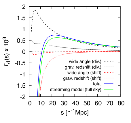
Figure 7: The four contributions to the dipole from the perturbative formula (65). Here ‘total’ is the sum of the divergence contributions ‘wide angle (div.)’ (RSD) and ‘grav. redshift (div.)’ [respectively the fourth and first term in Eq. (65)], and ’shift’ contributions [respectively the third and second term in Eq. (65), proportional to $\mathrm{d}\xi/\mathrm{d}s$]. For reference we have also plotted the nonperturbative dipole calculated from the streaming model (neglecting the connected piece in the covariance (7)). For the gravitational redshift curve there is a steep rise and fall near $s=0$ due to the NFW cusp. (note that each curve is an odd function so must go to zero at $s=0$, independent of model). Here $b_{A}=2$, $b_{B}=1$, and $z=0.341$.

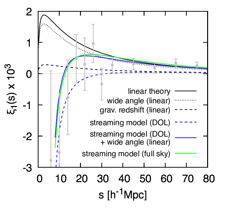
Figure 8: Impact of wide-angle effects on the linear and nonlinear dipoles at $z=0.341$. The linear-theory dipole (solid black) consists of the contribution from gravitational redshift (dashed black) and wide-angle effects in RSD (dotted black). The other three curves show various nonlinear models of the dipole: (i) dashed blue is the streaming model in the distant-observer limit (DOL) [Eq. (36)], in which only gravitational redshift contributes to the dipole and not RSD (since there are no wide-angle effects); (ii) solid blue is similar to model (i) but with the linear wide-angle correction added as a post-hoc correction; (iii) solid green is the streaming model in the wide-angle regime with RSD and gravitational redshift [see Eq. (9)]. Note that: none of these models include the effects of lookback time and lightcone; each of the linear-theory curves does not by definition contain normalisation from the density weighting; and the linear-theory curve of gravitational redshift is computed purely using linear theory, not the halo model (as used in Figure 7). For reference we show the measurements from the RayGal catalogues (for $M_{A}=2.2\times 10^{13}\,h^{-1}M_{\odot}$ and $M_{B}=0.28\times 10^{13}\,h^{-1}M_{\odot}$).

Computing $\partial_{a}\hskip 0.59998ptm_{[AB]}^{a}$ is more involved. For convenience, we split this into a part from RSD and a part from gravitational redshift:

$$\partial_{a}\hskip 0.59998ptm^{a}_{[AB]}\equiv\partial\cdot m_{[AB]}=\partial\cdot m^{\mathrm{RSD}}_{[AB]}+\partial\cdot m^{\mathrm{grav}}_{[AB]}\,.$$ (62)

In spherical coordinates the divergence is given by

$$\partial\cdot\hskip 0.59998ptm=\sum_{J=1,2}\frac{1}{\chi_{J}^{2}}\frac{\partial(\chi_{J}^{2}\,m^{J})}{\partial\chi_{J}}\,=\sum_{J=1,2}\left(\frac{\partial}{\partial\chi_{J}}+\frac{2}{\chi_{J}}\right)m^{J}\,,$$ (63)

where the sum is over the two radial components of $\bm{m}_{[AB]}$, see Eq. (11). The absence of the angular gradient on the right-hand side is because $\bm{m}_{AB}$ is purely radial.

The inverse-distance terms in the divergence formula (63) are wide-angle terms and so vanish when we take the distant-observer limit ($\epsilon\to 0$). This means that we only need to consider these types of terms for ${m}_{[AB]}^{\mathrm{RSD}}$ since for ${m}_{[AB]}^{\mathrm{grav}}$ these terms lead to corrections of order $\epsilon\hskip 0.59998pt\llangle\Delta\psi\rrangle\sim\epsilon^{2}$. In other words, we include wide-angle effects for RSD but not for gravitational redshift.

Substitution of the radial components (39) into the foregoing equation (63) then yields

$$\partial\cdot{m}^{\mathrm{RSD}}_{[AB]} =\left(\frac{\partial}{\partial\chi_{1}}+\frac{2}{\chi_{1}}\right)\mu_{1}\llangle\bar{u}\rrangle+\left(\frac{\partial}{\partial\chi_{2}}+\frac{2}{\chi_{2}}\right)\mu_{2}\llangle\bar{u}\rrangle\,,$$

$$\partial\cdot{m}^{\mathrm{grav}}_{[AB]} =\frac{1}{2}\frac{\partial}{\partial\chi_{1}}\llangle\Delta\psi\rrangle-\frac{1}{2}\frac{\partial}{\partial\chi_{2}}\llangle\Delta\psi\rrangle+\mathcal{O}(\epsilon^{2})\,,$$

where $\mu_{1}\equiv\hat{\mathbf{s}}\cdot\hat{\mathbf{n}}_{1}$ and $\mu_{2}\equiv\hat{\mathbf{s}}\cdot\hat{\mathbf{n}}_{2}$, and $\llangle\Delta\psi\rrangle$ and $\llangle\bar{u}\rrangle$ are evaluated at $r=s$. To extract the dipole we need to express each of these terms in coordinates $s,d,\mu$ using the coordinate relations given in Appendix I. After a short calculation, we find

$$\frac{3}{2}\int\mathrm{d}\mu\hskip 0.59998pt\mathcal{L}_{1}(\mu)\,\partial\cdot m^{\mathrm{RSD}}_{[AB]} =\epsilon\hskip 0.59998pt\frac{4}{5s^{4}}\frac{\mathrm{d}(s^{4}\llangle\bar{u}\rrangle)}{\mathrm{d}s}+\mathcal{O}(\epsilon^{2})\,,$$

$$\frac{3}{2}\int\mathrm{d}\mu\hskip 0.59998pt\mathcal{L}_{1}(\mu)\,\partial\cdot m^{\mathrm{grav}}_{[AB]} =\frac{\mathrm{d}\llangle\Delta\psi\rrangle}{\mathrm{d}s}+\mathcal{O}(\epsilon^{2})\,.$$ (64)

These are the linear dipoles due to RSD and gravitational redshift (although with a correction from the normalisation due to the density weighting). Note that the RSD dipole, given here in unusually compact form, is in fact equivalent to the well-known but lengthier expression (see Appendix G).

Finally, inserting Eqs. (61) and (64) into Eq. (59) we find for the total dipole

$$\xi_{1}(s,d)=-(1+\xi_{AB})\frac{\mathrm{d}\llangle\Delta\psi\rrangle}{\mathrm{d}s}-\llangle\Delta\psi\rrangle\hskip 0.59998pt\frac{\mathrm{d}\xi_{AB}}{\mathrm{d}s}$$ (65)

$$\quad-\epsilon\left(\frac{2}{5}\llangle\bar{u}\rrangle\frac{\mathrm{d}\xi_{AB}}{\mathrm{d}s}+(1+\xi_{AB})\frac{4}{5s^{4}}\frac{\mathrm{d}(s^{4}\llangle\bar{u}\rrangle)}{\mathrm{d}s}\right)+\mathcal{O}(\epsilon^{2})\,,$$

where we recall the dependence on $d$ enters only through $\epsilon=s/d$. This formula, expressed in terms of the pairwise functions, contains the well-known linear contribution from wide-angle RSD (last term) as well as the linear gravitational redshift, $\frac{\mathrm{d}}{\mathrm{d}s}\llangle\Delta\psi\rrangle_{{\color[rgb]{0.1,0.69,0.16}\rm lin}}\simeq(b_{A}-b_{B})\langle\frac{\partial\psi}{\partial\chi}\delta\rangle$ (first term). The other two terms (second and third terms) are second order in correlators and derive from $m_{AB}^{a}\hskip 0.59998pt\partial_{a}\hskip 0.59998pt\xi_{AB}\propto\frac{\mathrm{d}}{\mathrm{d}s}\xi_{AB}$. As a check, note that in the distant-observer limit ($\epsilon\to 0$) only the potential terms remain; the wide-angle RSD contributions, which here includes a second-order effect, vanishes as we expect.

VII.3 Discussion

Figure 7 shows the contributions from each term in Eq. (65). Both the RSD contribution and the gravitational redshift contributions are split into a linear contribution and a second-order contribution, that we denote by ‘shift’ since it arises from the shift term $m_{[AB]}^{a}\hskip 0.59998pt\partial_{a}\hskip 0.59998pt\xi_{(AB)}$ in Eq. (59). Note that the linear contributions are not strictly linear, due to the normalisation $1+\xi_{AB}$, as well as the intrinsic nonlinear terms within $\Delta\psi$ and $\bar{u}$.

Concerning the turnover in the dipole, we see from Figure 7 that the important term is due to the shift term in the gravitational redshift:

$$\xi_{1}(s,d)\supset-\llangle\Delta\psi\rrangle(s)\hskip 0.59998pt\frac{\mathrm{d}\hskip 0.59998pt\xi_{AB}}{\mathrm{d}s}\,.$$ (66)

The other shift contribution, due to wide-angle RSD, is proportional to $\llangle\bar{u}\hskip 0.59998pt\rrangle\frac{\mathrm{d}}{\mathrm{d}s}\xi_{AB}$, and, as Figure 7 shows, has negligible impact on the dipole. In the following, we call the gravitational redshift shift contribution simply ‘shift’ for simplicity.

Figure 7 shows that the shift gives a negative contribution to the dipole and rapidly grows in size towards small scales. Around $s\simeq 20\,h^{-1}\mathrm{Mpc}$ the shift begins to dominate over the other (net positive) contributions, which are driven mainly by the (linear) wide-angle effect. Eventually the shift cancels completely with the other contributions, leading to a sign change in the dipole.

The scale dependence of the shift (66) is mainly due to the slope of $\xi_{AB}$ and not from $\llangle\Delta\psi\rrangle$ itself. As we saw in Figure 6, $\llangle\Delta\psi\rrangle$ is relatively flat with mild scale dependence, vanishing as $r\to 0$. By contrast, $\xi_{AB}$ contains more small-scale power and so is increasingly steep towards small $r$, nonvanishing as $r\to 0$.

The amplitude of the shift (66) depends on both $\llangle\Delta\psi\rrangle$ and the slope of $\xi_{AB}$. There is however more uncertainty in the amplitude compared to the scale dependence due to the relative uncertainty of $\llangle\Delta\psi\rrangle$. As discussed in Section VI.3.2, $\llangle\Delta\psi\rrangle$ (as with pairwise velocity difference) is sensitive to nonlinearities in that the large-scale contributions tend to cancel out in the difference, bringing into relief the small-scale contributions which do not cancel. The one-point function $\langle\psi(0)\hskip 0.59998pt\delta_{A}(0)\rangle$ contained within is sensitive to small-scale modelling and corrections to the linear estimate of $\langle\psi(0)\hskip 0.59998pt\delta_{A}(0)\rangle$ can be large (from $50\%$ to $200\%$, depending on the mass of the tracers). Uncertainty in this quantity translates to uncertainty in the scale at which the turnover occurs—or whether it occurs at all. While we have assumed linear theory for $\xi_{AB}$, we have checked that improved modelling of $\xi_{AB}$ using the resummed Zel’dovich model [79, 54] leads only to small changes to the shape and size of the shift (66). These results suggest that efforts to improve the modelling of the dipole should focus on $\llangle\Delta\psi\rrangle$ and $\langle\psi(0)\hskip 0.59998pt\delta_{A}(0)\rangle$ contained therein.

Although not included in our modelling, we note that halo exclusion (that haloes cannot overlap) [80, 81] strongly affects the small-scale behaviour of $\xi_{AB}(r)$ and which we expect drives another turnover in the dipole around the exclusion scale $R_{\mathrm{exc}}=R_{\mathrm{vir,A}}+R_{\mathrm{vir,B}}$. We can understand this because $R_{\mathrm{exc}}$ demarcates two distinctly different regimes: for $r\gtrsim R_{\mathrm{exc}}$ we roughly have the power-law behaviour $\xi_{AB}(r)\propto(r/R_{\mathrm{exc}})^{-\gamma}$ with $\gamma>0$, whereas for $r<R_{\mathrm{exc}}$ we have that $\xi_{AB}(r)=-1$ (as required by the condition that the probability of finding a halo pair separated by less than $R_{\mathrm{exc}}$ is zero). This means that we must have a sign change in $\xi_{AB}$ and $\mathrm{d}\hskip 0.59998pt\xi_{AB}/\mathrm{d}s$, leading to a turnover in the dipole through Eq. (66).

Since the shift (66) does not vanish in the limit $\epsilon\to 0$ it must therefore be present in the distant-observer limit. This is confirmed by Figure 8, which shows the predicted dipole (dashed blue curve) of the standard streaming model in the distant-observer limit but with the inclusion of gravitational redshift [Eq. (36)]. The fact that the dipole is negative at small scales and then hovers slightly above zero at large scales tells us that it is driven primarily by the shift, as we expect. However, there is no longer a turnover because the large, positive contribution from wide-angle RSD is absent from this model. Interestingly, we find that we can restore the turnover using a hybrid model. In this model we take the dipole from the aforementioned standard streaming model (but generalised to include gravitational redshift), and add to it a post-hoc correction given by wide-angle dipole [Eq. (117)]. With this simple addition we recover the turnover and find better agreement with the simulations on scales $s>40\,h^{-1}\mathrm{Mpc}$. But this is not entirely unexpected because we know that at relatively high redshift ($z=0.341$) the wide-angle effects are in the perturbative regime and thus able to be accounted for using the first-order correction (see Figure 3). At lower redshifts such a hybrid approach will not be possible and the full model in the wide-angle regime will be needed.

VIII Conclusions

Gravitational redshift is a key observable for future galaxy surveys. Past works have shown that the mildly nonlinear regime of large-scale structure is well adapted to measure this effect, since the signal is boosted on these scales. But to properly isolate the gravitational redshift signal it is essential to have a robust model of this effect, as well as of all other effects that contribute to the correlation function at the same order.

In this work, we have shown that all such effects—namely, the order $\mathcal{H}/k$ relativistic effects—are captured by a simple formula (23). The two-point function is given by Eq. (28) and builds on the wide-angle generalisation of the streaming model developed in previous work [60]. We have formulated a complete model by incorporating into that framework the lightcone effect (Section III.2) and the gravitational redshift, our main interest in this work.

This work has focussed on nonlinear modelling of the dipole, the multipole most sensitive to the gravitational redshift. With our complete model we found that the gravitational redshift and the kinematic wide-angle effects are the two most important contributions to the dipole, supporting the earlier findings of Ref. [67]. The contributions from the lightcone and lookback-time effects are small but not negligible.

We saw that the dipole’s turnover at separation $s\simeq 20\,h^{-1}\mathrm{Mpc}$—a key feature marking a regime where the gravitational redshift begins to dominate over the kinematic contributions—is well accounted for in our model. From a perturbative expansion of the model, we showed that this behaviour is due to an advection-like effect (which we called the ‘shift’) whereby pairs of distinct galaxies ($A\neq B$) are asymmetrically transported along the lines of sight.

The important quantity driving this turnover is the pairwise potential difference $\llangle\Delta\psi\rrangle$. This quantity is sensitive to nonlinearities at all scales and is not well modelled by linear theory. There are several reasons for this. As with the pairwise velocity difference $\llangle\Delta u\rrangle$, the long-wavelength contributions to $\llangle\Delta\psi\rrangle$ tend to cancel out in the difference, leaving behind the small-scale nonlinearities. (In fact this cancellation should be more acute for $\llangle\Delta\psi\rrangle$ given that the potential is longer range, more sensitive to large-scale matter modes than the velocity field.)

We showed that the dominant contribution to $\llangle\Delta\psi\rrangle$ comes from the one-halo term (see Figure 6) and is driven in large part by the difference between $\langle n_{A}(\mathbf{x})\hskip 0.59998pt\psi(\mathbf{x})\rangle/\langle n_{A}(\mathbf{x})\rangle$ and $\langle n_{B}(\mathbf{x})\hskip 0.59998pt\psi(\mathbf{x})\rangle/\langle n_{B}(\mathbf{x})\rangle$, i.e. the difference between the density-weighted mean potential of each population. Unlike the velocity, the weighted potential does not average to zero: $\langle\delta_{A}(\mathbf{x})\mathbf{v}(\mathbf{x})\rangle=0$ whereas $\langle\delta_{A}(\mathbf{x})\hskip 0.59998pt\psi(\mathbf{x})\rangle\neq 0$ (and likewise for $B$). This follows from the fact that, under isotropy, we are as likely to sample both positive and negative velocities (both redshift or blueshift) in equal measure. This is true for both the coherent velocities on large scales and for the random virial motions on small scales: sampled over sufficiently large volumes velocities have no preferred directions, $\langle\delta_{A}(\mathbf{x})\mathbf{v}(\mathbf{x})\rangle=0$. By contrast $\langle\delta_{A}(\mathbf{x})\hskip 0.59998pt\psi(\mathbf{x})\rangle$ tends to have a definite sign. Since the density weighting biases the potential towards overdense collapsed regions, we will tend to see the effect of a gravitational redshift, not a gravitational blueshift. Thus, $\llangle\Delta\psi\rrangle$ is sensitive to the immediate environment through the local potential in which the tracers reside.

The importance of a nonlinear ingredient to capture the turnover of the dipole at small scales has been pointed out in previous works [47, 48]. In Ref. [47], an EFT-like nuisance parameter is added to the modelling of the power spectrum dipole, and fitted from the simulations. In Ref. [48], a constant nonlinear potential contribution is added to the displacement field of each of the tracers. In this work, we showed how this nonlinear ingredient naturally arises, namely, through the density-weighted pairwise potential difference $\llangle\Delta\psi\rrangle$, which we estimated using the halo model.

Besides these findings on the gravitational redshift, we found in the course of our calculations that redshift-space correlations find their natural expression in terms of pairwise correlation functions, whether in the distant-observer limit or the wide-angle regime. We found, for example, that the dipole generated by RSD takes on a particularly compact form in terms of the pairwise mean velocity. These quantities each have distinct physical meaning and contain information about stochastic effects, such as drift and FoG dispersion, that are absent in more straightforward perturbative treatments. Moreover, these scalar quantities carry parity: either symmetric or anti-symmetric under pair exchange of distinct tracers (and only symmetric in the case of identical tracers). We saw that such properties underlie the more conventional way of identifying anti-symmetric correlations (in terms of derivative counting), and that these functions provide a convenient way to build up the multipoles perturbatively. On large scales (terms linear in correlators), the symmetric functions contribute to the even multipoles, while the anti-symmetric functions contribute to the odd multipoles. On smaller scales (terms quadratic or higher in correlators), one counts all products of the pairwise functions which are overall symmetric or anti-symmetric as contributing to the even or odd multipoles, respectively.

Finally, let us mention a few ways in which our model can be improved.

1. An obvious starting point is the extension of the gravitational evolution and tracer bias beyond linear theory. A better approach would be to use, for example, convolution Lagrangian perturbation theory [79, 54] to compute all the density-weighted correlations.

2. This work used haloes as tracers, as per the RayGal catalogues, but a more realistic application should extend the modelling to galaxies. This implies an important change in the modelling of the pairwise potential difference. Since galaxies do not necessarily lie at the centre of haloes $\llangle\Delta\psi\rrangle$ needs to be recalculated to account for this offset (e.g. through modelling of the halo occupation statistics).

3. Inclusion of magnification and evolution bias is another obvious area of improvement. As we showed in previous work [60], these selection effects enter through a change in the density weighting in a similar way to the lightcone correction so should be straightforward to include in the model.

4. It would be interesting to investigate the impact of non-Gaussian cumulants on the dipole (in analogy with Ref. [82]). If the first cumulant (the mean) is important for the anti-symmetric correlations, as we found in this work, then it might reasonably be expected that the third cumulant (the skew) is the next most relevant. In this context, numerical simulations of the pairwise statistics of the potential difference and a study of the scale-dependent distribution should better inform further improvements to the modelling. We leave these aspects for future work.

Appendix A An alternative way to model $p(\bm{\chi}\,|\,\bm{\chi}^{\prime})$

This appendix outlines an alternative strategy for obtaining the transition probability $p(\bm{\chi}\,|\,\bm{\chi}^{\prime})$ and with it the correlation function $\xi^{\mathrm{(s)}}$. The basic idea is to use the chain rule to reduce $p(\bm{\chi}\,|\,\bm{\chi}^{\prime})$ to the product of two distributions, from RSD and gravitational redshift, with the assumption that each effect is largely independent of the other. This amounts to ignoring the correlations between velocity and potential—a good approximation in the case of the dipole (see Section V).

Without making any assumptions about $p(\bm{\chi}\,|\,\bm{\chi}^{\prime})$, we insert Eq. (16) into the correlation function (4) to get

$$1+\xi^{(\mathrm{s})}(\bm{\chi}) =\frac{1}{\chi_{1}^{2}\,\chi_{2}^{2}}\int\mathrm{d}\chi_{1}^{\prime}\,\chi_{1}^{\prime 2}\int\mathrm{d}\chi_{2}^{\prime}\,\chi_{2}^{\prime 2}\hskip 0.59998pt[1+\xi(\bm{\chi}^{\prime})]\hskip 0.59998ptp(\bm{\chi}\,|\,\bm{\chi}^{\prime})$$

$$=\frac{1}{\chi_{1}^{2}\,\chi_{2}^{2}}\int\mathrm{d}\chi_{1}^{\prime}\,\chi_{1}^{\prime 2}\int\mathrm{d}\chi_{2}^{\prime}\,\chi_{2}^{\prime 2}\hskip 0.59998pt[1+\xi(\bm{\chi}^{\prime})]\int\mathrm{d}^{2}\bm{\chi}^{\prime\prime}p_{\mathrm{grav}}(\bm{\chi}\,|\,\bm{\chi}^{\prime\prime},\bm{\chi}^{\prime})\hskip 0.59998ptp_{\mathrm{RSD}}(\bm{\chi}^{\prime\prime}\,|\,\bm{\chi}^{\prime})\,,$$ (67)

where $\mathrm{d}^{2}\bm{\chi}^{\prime\prime}=\mathrm{d}\chi_{1}^{\prime\prime}\mathrm{d}\chi_{2}^{\prime\prime}$. The crucial assumption that we will now make is that the transitions are a Markov process so that the current state only depends on the immediate previous state, or $p_{\mathrm{grav}}(\bm{\chi}\,|\,\bm{\chi}^{\prime\prime},\bm{\chi}^{\prime})=p_{\mathrm{grav}}(\bm{\chi}\,|\,\bm{\chi}^{\prime\prime})$. This allows us to separate the integral over the initial positions $\bm{\chi}^{\prime}$ from the integral over the intermediate positions $\bm{\chi}^{\prime\prime}$. Indeed, by rearranging the integrand in Eq. (67) we can write

$$1+\xi^{(\mathrm{s})}(\bm{\chi}) =\frac{1}{\chi_{1}^{2}\,\chi_{2}^{2}}\int\mathrm{d}^{2}\bm{\chi}^{\prime\prime}\chi_{1}^{\prime\prime 2}\hskip 0.59998pt\chi_{2}^{\prime\prime 2}\left(\,\frac{1}{\chi_{1}^{\prime\prime 2}\hskip 0.59998pt\chi_{2}^{\prime\prime 2}}\int\mathrm{d}^{2}\bm{\chi}^{\prime}\chi_{1}^{\prime 2}\hskip 0.59998pt\chi_{2}^{\prime 2}\hskip 0.59998pt[1+\xi(\bm{\chi}^{\prime})]\hskip 0.59998ptp_{\mathrm{RSD}}(\bm{\chi}^{\prime\prime}\,|\,\bm{\chi}^{\prime})\right)p_{\mathrm{grav}}(\bm{\chi}\,|\,\bm{\chi}^{\prime\prime})\,.$$ (68)

Notice that this expression has a self-similar composition in that the inner integral has the same form as the outer integral. Thus defining $1+\xi_{\mathrm{RSD}}(\bm{\chi}^{\prime\prime})$ by the contents of the parentheses, we can write Eq. (68) as

$$1+\xi^{(\mathrm{s})}(\bm{\chi})=\frac{1}{\chi_{1}^{2}\hskip 0.59998pt\chi_{2}^{2}}\int\mathrm{d}^{2}\bm{\chi}^{\prime\prime}\chi_{1}^{\prime\prime 2}\hskip 0.59998pt\chi_{2}^{\prime\prime 2}\hskip 0.59998pt\big{[}1+\xi_{\mathrm{RSD}}(\bm{\chi}^{\prime\prime})\big{]}\hskip 0.89996ptp_{\mathrm{grav}}(\bm{\chi}\,|\,\bm{\chi}^{\prime\prime})\,.$$ (69)

In fact, this nested form holds for any number of transitions, provided the Markov property holds for each. This means that a series of transitions can be modelled by applying successive integral transformations to the base real-space correlation $1+\xi(\bm{\chi}^{\prime})$. The practical advantage is that the correlation function $1+\xi^{\mathrm{(s)}}$ (due to both RSD and gravitational redshift) can be obtained by simply applying a transformation to an existing, well-tested model of $1+\xi_{\mathrm{RSD}}$ (promoted to the wide-angle regime), i.e. by convolving it with the distribution $p_{\mathrm{grav}}(\bm{\chi}\,|\,\bm{\chi}^{\prime\prime})$. In this way the problem of modelling RSD is separated from the problem of modelling the gravitational redshift, which boils down to modelling the distribution for the pairwise potential (and which in a further approximation may be modelled in the distant-observer limit as a one-dimensional probability distribution; see Section VII).

An obvious assumption one can make in the modelling is to suppose that both $p_{\mathrm{RSD}}(\bm{\chi}^{\prime\prime}\,|\,\bm{\chi}^{\prime})$ and $p_{\mathrm{grav}}(\bm{\chi}\,|\,\bm{\chi}^{\prime\prime})$ are Gaussian. We will not investigate in any detail the validity of this assumption, except to note here that the marginal integral (16) for $p(\bm{\chi}\,|\,\bm{\chi}^{\prime})$ does not evaluate to an exact Gaussian, as one might presume, because of the non-trivial dependence on $\bm{\chi}^{\prime\prime}$ through $\bm{m}_{\mathrm{grav}}(\bm{\chi}^{\prime\prime})$ and $\mathbf{C}_{\mathrm{grav}}(\bm{\chi}^{\prime\prime})$ preventing analytic integration. Certainly it does not integrate to the two-dimensional Gaussian we have used in, e.g. Eq. (9). However, the full numerical result turns out be to close to the analytic Gaussian result obtained by simply replacing $\bm{m}_{\mathrm{grav}}(\bm{\chi}^{\prime\prime})\to\bm{m}_{\mathrm{grav}}(\bm{\chi})$ and $\mathbf{C}_{\mathrm{grav}}(\bm{\chi}^{\prime\prime})\to\mathbf{C}_{\mathrm{grav}}(\bm{\chi})$, where corrections to this approximation are small because displacements $\bm{\chi}-\bm{\chi}^{\prime\prime}$ are small compared with the configuration size $\bm{\chi}$ itself.

Alternatively, one may wish to simply take $p_{\mathrm{grav}}(\bm{\chi}\,|\,\bm{\chi}^{\prime\prime})=\delta_{\mathrm{D}}(\bm{\chi}-\bm{\chi}^{\prime\prime}-\bm{m}_{\mathrm{grav}}(\bm{\chi}^{\prime\prime}))$ (obtained by neglecting all but the first cumulant in the cumulant expansion of Eq. (5)), on the basis that the covariance is symmetric at leading order so unimportant for the dipole (see Section VI).

A.1 Redshift-space distortions as a dynamical equation and the $\lambda$ trick

In Sections II.3 and VII we alluded to a dynamical way of viewing RSD; here we give further support for this picture.

Introduce an auxiliary variable $\lambda$ and consider the map $\mathbf{s}(\mathbf{x},\lambda)=\mathbf{x}+\lambda\hskip 0.59998pt\delta\mathbf{x}(\mathbf{x})$ which smoothly interpolates between real space ($\lambda=0$) and redshift space ($\lambda=1$). Define the $\lambda$ density [cf. Eq. (3)]

$$n_{\lambda}(\mathbf{s},\lambda)\equiv\int\mathrm{d}^{3}\mathbf{x}\,n(\mathbf{x})\hskip 0.89996pt\delta_{\mathrm{D}}\big{[}\mathbf{s}-\mathbf{x}-\lambda\hskip 0.89996pt\delta\mathbf{x}(\mathbf{x})\big{]}\,,$$ (70)

so that we recover the redshift-space density $n_{\lambda}(\mathbf{s},\lambda=1)=n^{\mathrm{(s)}}(\mathbf{s})$ when $\lambda=1$, and the real-space density $n_{\lambda}(\mathbf{s},\lambda=0)=n(\mathbf{s})=n(\mathbf{x})$ when $\lambda=0$. To highlight the novelty in the following calculation let us restrict to RSD only, so $\delta\mathbf{x}(\mathbf{x})=\mathbf{u}_{\|}(\mathbf{x})\equiv\hat{\mathbf{n}}\cdot\mathbf{u}(\mathbf{x})\hskip 0.59998pt\hat{\mathbf{n}}$. Now differentiate Eq. (70) with respect to $\lambda$:

$$\frac{\partial}{\partial\lambda}\,n_{\lambda}(\mathbf{s},\lambda)=\int\mathrm{d}^{3}\mathbf{x}\,n(\mathbf{x})\,\frac{\partial}{\partial\lambda}\int\frac{\mathrm{d}^{3}\mathbf{k}}{(2\pi)^{3}}\,\mathrm{e}^{-\mathrm{i}\mathbf{k}\cdot[\mathbf{s}-\mathbf{x}-\lambda\hskip 0.49164pt\mathbf{u}_{\|}(\mathbf{x})]} =\int\mathrm{d}^{3}\mathbf{x}\,n(\mathbf{x})\hskip 0.89996pt\mathbf{u}_{\|}(\mathbf{x})\cdot\int\frac{\mathrm{d}^{3}\mathbf{k}}{(2\pi)^{3}}\,\mathrm{i}\mathbf{k}\,\mathrm{e}^{-\mathrm{i}\mathbf{k}\cdot[\mathbf{s}-\mathbf{x}-\lambda\hskip 0.49164pt\mathbf{u}_{\|}(\mathbf{x})]}$$

$$=-\int\mathrm{d}^{3}\mathbf{x}\,n(\mathbf{x})\hskip 0.89996pt\mathbf{u}_{\|}(\mathbf{x})\cdot\frac{\partial}{\partial\mathbf{s}}\,\delta_{\mathrm{D}}\big{[}\mathbf{s}-\mathbf{x}-\lambda\hskip 0.59998pt\mathbf{u}_{\|}(\mathbf{x})\big{]}\,,$$ (71)

where in the first equality we used the Fourier representation of the delta function, and in the last equality we exchanged the factor of $\mathrm{i}\mathbf{k}$ for an overall derivative in $\mathbf{s}$.

Equation (71) is an expression of number conservation, for if we define the $\lambda$ momentum field [cf. Eq. (70)]

$$\mathbf{p}_{\|}(\mathbf{s},\lambda)\equiv\int\mathrm{d}^{3}\mathbf{x}\,n(\mathbf{x})\hskip 0.89996pt\mathbf{u}_{\|}(\mathbf{x})\hskip 0.89996pt\delta_{\mathrm{D}}\big{[}\mathbf{s}-\mathbf{x}-\lambda\hskip 0.59998pt\mathbf{u}_{\|}(\mathbf{x})\big{]}\,,$$ (72)

(where the redshift-space momentum field is recovered when $\lambda=1$), then we can write Eq. (71) as

$$\frac{\partial}{\partial\lambda}\,n_{\lambda}(\mathbf{s},\lambda)+\frac{\partial}{\partial\hskip 0.59998pt\mathbf{s}}\cdot\mathbf{p}_{\|}(\mathbf{s},\lambda)=0\,.$$ (73)

With $\lambda$ acting as a time parameter, this can be viewed as a continuity equation. As we let time go from $\lambda=0$ to $\lambda=1$ this equation tells us how the real-space density continuously distorts into the redshift-space density. Note that $\mathbf{p}_{\|}^{\mathrm{(s)}}$, like $\mathbf{u}_{\|}$, is a purely radial field.

We can use the continuity equation to obtain the redshift-space analogue of the pairwise conservation equation [56]. By evaluating Eq. (73) at $\mathbf{s}_{1}$, multiplying through by $n_{\lambda}$ evaluated at $\mathbf{s}_{2}$, then adding to it the same equation but with $\mathbf{s}_{1}\leftrightarrow\mathbf{s}_{2}$, we obtain

$$\frac{\partial}{\partial\lambda}\big{\langle}n_{\lambda}(\mathbf{s}_{1},\lambda)\hskip 0.59998ptn_{\lambda}(\mathbf{s}_{2},\lambda)\big{\rangle}+\mu\hskip 0.89996pt\frac{\partial}{\partial s_{z}}\big{[}\big{\langle}n_{\lambda}(\mathbf{s}_{1},\lambda)\hskip 0.59998ptn_{\lambda}(\mathbf{s}_{2},\lambda)\big{\rangle}\hskip 0.59998pt\llangle\Delta u\rrangle_{\lambda}\big{]}=0\,,$$ (74)

where $\partial/\partial s_{z}=\hat{\mathbf{z}}\cdot\partial/\partial\hskip 0.59998pt\mathbf{s}$, $\mu=\hat{\mathbf{s}}\cdot\hat{\mathbf{z}}$ (with line of sight along $z$ direction), $\mathbf{s}=\mathbf{s}_{1}-\mathbf{s}_{2}$ and $\llangle\Delta u\rrangle_{\lambda}$ is the $\lambda$ pairwise velocity difference (density weighting given by $n_{\lambda}$). Since the separation of pairs orthogonal to the line of sight ($\mu=0$) do not evolve under the corresponding correlations are undistorted, as we can see from Eq. (74). Note that here we have assumed the distant-observer limit wherein the Eq. (74) takes a simple form; in the wide-angle regime there is an additional term with dependence on the pairwise mean velocity (see Section VI.2).

Since we have touched on the redshift-space momentum field, a prospective cosmological probe [83, 84, 85, 86], let us note here that if we have a model or ansatz for the redshift-space density we can use the continuity equation (73) to solve for the redshift-space momentum, that is, without having to use Eq. (72) to model $\mathbf{p}^{\mathrm{(s)}}_{\|}(\mathbf{s})$ from scratch. This means that if we have a model of the density correlations (e.g. Eq. (9)), a model of the momentum correlations can in principle be ‘generated’ from it using the above $\lambda$ trick. More precisely, by solving Eq. (73) by Green’s method we obtain the redshift-space momentum field $\mathbf{p}^{\mathrm{(s)}}_{\|}(\mathbf{s})=\mathbf{p}_{\|}(\mathbf{s},\lambda=1)$ as

$$\mathbf{p}^{\mathrm{(s)}}_{\|}(\mathbf{s}) =-\frac{\partial}{\partial\lambda}\int\mathrm{d}^{3}\mathbf{y}\hskip 0.89996pt\frac{(\mathbf{s}-\mathbf{y})}{4\pi\hskip 0.59998pt|\hskip 0.59998pt\mathbf{s}-\mathbf{y}|^{3}}\hskip 0.89996ptn_{\lambda}(\mathbf{y},\lambda)\,\Big{|}_{\lambda=1}=\frac{\partial}{\partial\lambda}\left(\frac{\partial}{\partial\hskip 0.59998pt\mathbf{s}}\int\mathrm{d}^{3}\mathbf{y}\,G(\mathbf{s}-\mathbf{y})\,n_{\lambda}(\mathbf{y},\lambda)\right)\bigg{|}_{\lambda=1}\,,$$ (75)

where $G(\mathbf{s}-\mathbf{y})=1/4\pi\hskip 0.59998pt|\hskip 0.59998pt\mathbf{s}-\mathbf{y}|$ and we used that $\mathbf{p}_{\|}^{\mathrm{(s)}}$ has no curl component [86] so is able to be written as the gradient of a scalar. The two-point correlation function of the radial momentum $p_{\|}^{\mathrm{(s)}}=\mathbf{p}_{\|}^{\mathrm{(s)}}\cdot\hat{\mathbf{n}}$ is then

$$\big{\langle}p_{\|}^{\mathrm{(s)}}(\mathbf{s}_{1})\hskip 0.59998ptp_{\|}^{\mathrm{(s)}}(\mathbf{s}_{2})\big{\rangle}=\frac{\partial}{\partial\lambda_{1}}\frac{\partial}{\partial\lambda_{2}}\int\mathrm{d}^{3}\mathbf{y}_{1}\hskip 0.89996pt\frac{\partial}{\partial s_{1}}G(\mathbf{s}_{1}-\mathbf{y}_{1})\int\mathrm{d}^{3}\mathbf{y}_{2}\hskip 0.89996pt\frac{\partial}{\partial s_{2}}G(\mathbf{s}_{2}-\mathbf{y}_{2})\,\big{\langle}n_{\lambda}(\mathbf{y}_{1},\lambda_{1})\hskip 0.59998ptn_{\lambda}(\mathbf{y}_{2},\lambda_{2})\big{\rangle}\,\Big{|}_{\lambda_{1}=\lambda_{2}=0}\,,$$ (76)

where $\chi_{1}=|\mathbf{s}_{1}|=\mathbf{s}_{1}\cdot\hat{\mathbf{n}}_{1}$ and $\chi_{2}=|\mathbf{s}_{2}|=\mathbf{s}_{2}\cdot\hat{\mathbf{n}}_{2}$. This formula expresses the redshift-space momentum correlations in terms of the redshift-space density correlations. It is valid in the full wide-angle regime. Since the relation between the momentum (or velocity) and the density is nonlocal so too is the relation between their correlations. This means that the momentum correlation at a given separation is determined by density correlations from a range of separations. We thus run into the problem of needing to integrate down to arbitrarily small separations, where the model of the density correlations breaks down. Furthermore, for wide-angle correlations one needs to contend with high-dimensional integration. We note however that in the distant-observer limit one can reduce Eq. (76) to a one-dimensional integral over the line-of-sight separation.

Appendix B Correlation functions

Here we list and give explicit formulae for all real-space correlation functions that constitute the redshift-space correlation function (28). These enter through the normalisation $1+\xi_{AB}$, the mean $\bm{m}$ [Eq. (11)], and the covariance $\mathbf{C}$ [Eq. (13)]. We will work at leading order, keeping only leading-order statistics such as $\langle u_{\|}(\mathbf{x}_{1})\hskip 0.59998ptu_{\|}(\mathbf{x}_{2})\rangle$, neglecting third- and fourth-order statistics such as $\langle u_{\|}(\mathbf{x}_{1})\hskip 0.59998ptu_{\|}(\mathbf{x}_{2})\hskip 0.59998pt\delta_{A}(\mathbf{x}_{1})\rangle$ and $\langle u_{\|}(\mathbf{x}_{1})\hskip 0.59998ptu_{\|}(\mathbf{x}_{2})\hskip 0.59998pt\delta_{A}(\mathbf{x}_{1})\hskip 0.59998pt\delta_{B}(\mathbf{x}_{2})\rangle$. The components of $\bm{m}_{\mathrm{RSD}}$ and $\mathbf{C}_{\mathrm{RSD}}$ then read

$$\llangle u_{\|}(\mathbf{x}_{1})\rrangle \simeq\big{[}1+\xi_{AB}(\mathbf{x}_{1},\mathbf{x}_{2})\big{]}^{-1}\hat{n}_{1}^{i}\big{\langle}u_{i}(\mathbf{x}_{1})\hskip 0.59998pt\tilde{\delta}_{B}(\mathbf{x}_{2})\big{\rangle}\,,$$ (77)

$$\llangle u_{\|}(\mathbf{x}_{1})\hskip 0.59998ptu_{\|}(\mathbf{x}_{2})\rrangle \simeq\big{[}1+\xi_{AB}(\mathbf{x}_{1},\mathbf{x}_{2})\big{]}^{-1}\hat{n}_{1}^{i}\hat{n}_{2}^{j}\big{\langle}u_{i}(\mathbf{x}_{1})\hskip 0.59998ptu_{j}(\mathbf{x}_{2})\big{\rangle}\,,$$ (78)

while the components of $\bm{m}_{\mathrm{grav}}$, $\mathbf{C}_{\mathrm{grav}}$, and $\mathbf{C}_{\mathrm{cross}}$ respectively read

$$\llangle\psi(\mathbf{x}_{1})-\psi_{O}\rrangle \simeq\big{[}1+\xi_{AB}(\mathbf{x}_{1},\mathbf{x}_{2})\big{]}^{-1}\big{\langle}[\psi(\mathbf{x}_{1})-\psi_{O}][\tilde{\delta}_{A}(\mathbf{x}_{1})+\tilde{\delta}_{B}(\mathbf{x}_{2})]\big{\rangle}\,,$$ (79)

$$\llangle[\psi(\mathbf{x}_{1})-\psi_{O}][\psi(\mathbf{x}_{2})-\psi_{O}]\rrangle \simeq\big{[}1+\xi_{AB}(\mathbf{x}_{1},\mathbf{x}_{2})\big{]}^{-1}\big{\langle}[\psi(\mathbf{x}_{1})-\psi_{O}][\psi(\mathbf{x}_{2})-\psi_{O}]\big{\rangle}\,,$$ (80)

$$\llangle[\psi(\mathbf{x}_{1})-\psi_{O}]\hskip 0.59998ptu_{\|}(\mathbf{x}_{2})\rrangle \simeq\big{[}1+\xi_{AB}(\mathbf{x}_{1},\mathbf{x}_{2})\big{]}^{-1}\hat{n}_{2}^{j}\big{\langle}[\psi(\mathbf{x}_{1})-\psi_{O}]\hskip 0.59998ptu_{j}(\mathbf{x}_{2})\big{\rangle}\,.$$ (81)

Here $\tilde{\delta}_{A}(\mathbf{x}_{1})=\delta_{A}(\mathbf{x}_{1})+\mathbf{v}(\mathbf{x}_{1})\cdot\hat{\mathbf{n}}_{1}$ and $\tilde{\delta}_{B}(\mathbf{x}_{2})=\delta_{B}(\mathbf{x}_{2})+\mathbf{v}(\mathbf{x}_{2})\cdot\hat{\mathbf{n}}_{2}$ (including the lightcone correction). Moreover, we will assume linear theory so $\delta_{A}=b_{A}\hskip 0.59998pt\delta$ and $\delta_{B}=b_{B}\hskip 0.59998pt\delta$, with $\delta$ the linear matter field, and $b_{A}$ and $b_{B}$ the linear biases. Note that the normalisation $1+\xi_{AB}(\mathbf{x}_{1},\mathbf{x}_{2})$ [which also includes the lightcone correction; see Eq. (27)] becomes important on small scales and is always retained in numerical work. In addition to $\xi_{AB}$, there are six other correlation functions needed.

Velocity correlations. The correlations needed for RSD can be constructed by taking line-of-sight projections of the basic vector and tensor correlations, $\langle u_{i}(\mathbf{x}_{1})\hskip 0.59998pt\delta(\mathbf{x}_{2})\rangle$ and $\langle u_{i}(\mathbf{x}_{1})\hskip 0.59998ptu_{j}(\mathbf{x}_{2})\rangle$. By statistical isotropy, these basic correlations have the general forms $\langle u_{i}(\mathbf{x}_{1})\hskip 0.59998pt\delta(\mathbf{x}_{2})\rangle=\xi_{u\hskip 0.49164pt\delta}(r)\hskip 0.59998pt\hat{r}_{i}$ and $\langle u_{i}(\mathbf{x}_{1})\hskip 0.59998ptu_{j}(\mathbf{x}_{2})\rangle=\xi_{u\hskip 0.49164ptu}^{\hskip 0.49164pt\|}(r)\hat{r}_{i}\hat{r}_{j}+\xi_{u\hskip 0.49164ptu}^{\perp}(r)(\delta_{ij}-\hat{r}_{i}\hat{r}_{j})$, i.e. they can be written in terms of scalar correlations $\xi_{u\hskip 0.49164pt\delta}(r)$, $\xi_{u\hskip 0.49164ptu}^{\|}(r)$, and $\xi_{u\hskip 0.49164ptu}^{\perp}(r)$. According to gravitational instability theory, the growing mode is vorticity free so we can write $u_{i}$ solely in terms of the (scaled) velocity divergence $\theta=\nabla_{i}u^{i}$ so $u_{i}=\mathrm{i}k_{i}/k^{2}\theta$ (where $\theta$ has the same units as $\delta$). In terms of the power spectra of $\delta$ and $\theta$, the scalar correlation functions are obtained through contractions with the unit separation $\hat{\mathbf{r}}$:

$$\xi_{u\hskip 0.49164pt\delta}(r)\equiv\hat{r}^{i}\big{\langle}u_{i}(\mathbf{x}_{1})\hskip 0.59998pt\delta(\mathbf{x}_{2})\big{\rangle} =\frac{1}{\mathcal{H}}\int\frac{k^{2}\mathrm{d}k}{2\pi^{2}}\,\left(\frac{\mathcal{H}}{k}\right)\hskip 0.89996ptj_{1}(kr)\hskip 0.59998ptP_{\theta\delta}(k)\,,$$ (83)

$$\xi_{u\hskip 0.49164ptu}^{\hskip 0.49164pt\|}(r)\equiv\hat{r}^{i}\hskip 0.59998pt\hat{r}^{j}\big{\langle}u_{i}(\mathbf{x}_{1})\hskip 0.59998ptu_{j}(\mathbf{x}_{2})\big{\rangle} =\frac{1}{\mathcal{H}^{2}}\int\frac{k^{2}\mathrm{d}k}{2\pi^{2}}\left(\frac{\mathcal{H}}{k}\right)^{2}K_{\|}(kr)\hskip 0.59998ptP_{\theta\theta}(k)\,,$$ (84)

$$\xi_{u\hskip 0.49164ptu}^{\perp}(r)\equiv\frac{1}{2}\mathcal{P}_{\perp}^{\hskip 0.49164ptki}\,\mathcal{P}_{\perp}^{\hskip 0.49164ptkj}\hskip 0.59998pt\big{\langle}u_{i}(\mathbf{x}_{1})\hskip 0.59998ptu_{j}(\mathbf{x}_{2})\big{\rangle} =\frac{1}{\mathcal{H}^{2}}\int\frac{k^{2}\mathrm{d}k}{2\pi^{2}}\left(\frac{\mathcal{H}}{k}\right)^{2}K_{\perp}(kr)\hskip 0.59998ptP_{\theta\theta}(k)\,.$$ (85)

Note these depend on $r$ only and the dimensions of these correlations (as well as those below) are given by the prefactor $1/\mathcal{H}^{n}$ (e.g. $\xi_{u\hskip 0.49164pt\delta}$ has units length and $\xi_{u\hskip 0.49164ptu}^{\perp}$ units length squared). Here $K_{\|}(x)=j_{0}(x)/3-2j_{2}(x)/3$ and $K_{\perp}(x)=j_{0}(x)/3+j_{2}(x)/3$ are the standard velocity kernels [87], and we have defined the projection tensor $\mathcal{P}^{\perp}_{ij}=\delta_{ij}-\hat{r}_{i}\hat{r}_{j}$ which we used to extract the part perpendicular to $\hat{r}$. The power spectra are defined as usual as $\langle\delta(\mathbf{k})\hskip 0.59998pt\delta(\mathbf{k}^{\prime})\rangle=(2\pi)^{3}\delta_{\mathrm{D}}(\mathbf{k}+\mathbf{k}^{\prime})P_{\delta\delta}(k)$, $\langle\theta(\mathbf{k})\hskip 0.59998pt\delta(\mathbf{k}^{\prime})\rangle=(2\pi)^{3}\delta_{\mathrm{D}}(\mathbf{k}+\mathbf{k}^{\prime})P_{\theta\delta}(k)$, and $\langle\theta(\mathbf{k})\hskip 0.59998pt\theta(\mathbf{k}^{\prime})\rangle=(2\pi)^{3}\delta_{\mathrm{D}}(\mathbf{k}+\mathbf{k}^{\prime})P_{\theta\theta}(k)$. Note that the odd-parity correlations (those containing an odd power of $\hat{r}$) have Bessel functions of odd order, while even-parity correlations have Bessel functions of even order. This means that, unlike the even-parity correlations, the odd-parity correlations vanish at $r=0$.

These formulae are independent of the modelling of $\delta$ and $\theta$. In this work we use linear theory so $\theta\simeq-f\delta$, with $f$ the linear growth rate. The above formulae can then be written in terms of the linear matter power spectrum $P_{\mathrm{lin}}$, with $P_{\theta\delta}\simeq-fP_{\mathrm{lin}}$ and $P_{\theta\theta}\simeq f^{2}P_{\mathrm{lin}}$.

Potential correlations. With the inclusion of gravitational redshift, the mean displacement $\bm{m}$ now contains a correlation between $\psi$ and $\delta$ (due to the density weighting). Working on subhorizon scales, we use Poisson’s equation $\nabla^{2}\Psi=4\pi Ga^{2}\bar{\rho}\delta=\frac{3}{2}\hskip 0.89996pt\Omega_{m}\mathcal{H}^{2}\delta$ to write $\xi_{\psi\delta}(r)=\langle\psi(\mathbf{x}_{1})\hskip 0.59998pt\delta(\mathbf{x}_{2})\rangle$ in terms of the matter power spectrum as

$$\xi_{\psi\delta}(r)\equiv\big{\langle}\psi(\mathbf{x}_{1})\hskip 0.59998pt\delta(\mathbf{x}_{2})\big{\rangle} =\frac{1}{\mathcal{H}}\frac{3\Omega_{m}}{2}\int\frac{k^{2}\mathrm{d}k}{2\pi^{2}}\left(\frac{\mathcal{H}}{k}\right)^{2}j_{0}(kr)P_{\delta\delta}(k)\,,$$ (86)

where $\Omega_{m}=\Omega_{m}(z)$ is the fractional matter density. Note that $\psi$ and $\delta$ are positively correlated due to our convention $\psi=-\mathcal{H}^{-1}\Psi$, so $\xi_{\psi\delta}(r)>0$ for all $r$. This term is order $(\mathcal{H}/k)^{2}$, as with $\langle u^{2}\rangle$. There is also a one-point contribution, $\xi_{\psi\delta}(0)$, which does not vanish, unlike $\xi_{u\hskip 0.49164pt\delta}(0)$ which does for reasons of symmetry.

The covariance $\mathbf{C}_{\mathrm{cross}}$ [Eq. (13c)] contains correlations between $u$ and $\psi$. Because of the density weighting there are also correlations with $\delta$, but these enter at lowest order in the form of an integrated bispectrum (proportional to $P_{\mathrm{lin}}^{2}$). We will neglect such contributions. Thus for $\mathbf{C}_{\mathrm{cross}}$ we need only $\langle u_{i}(\mathbf{x}_{1})\hskip 0.59998pt\psi(\mathbf{x}_{2})\rangle=\xi_{u\hskip 0.49164pt\psi}(r)\hskip 0.59998pt\hat{r}_{i}$, where $\xi_{u\hskip 0.49164pt\psi}(r)$ is given by

$$\xi_{u\hskip 0.49164pt\psi}(r)\equiv\hat{r}^{i}\big{\langle}u_{i}(\mathbf{x}_{1})\hskip 0.59998pt\psi(\mathbf{x}_{2})\big{\rangle} =\frac{1}{\mathcal{H}^{2}}\frac{3\Omega_{m}}{2}\int\frac{k^{2}\mathrm{d}k}{2\pi^{2}}\left(\frac{\mathcal{H}}{k}\right)^{3}j_{1}(kr)P_{\theta\delta}(k)\,,$$ (87)

where again we have used that $u_{i}$ is a gradient flow. Note that compared with Eq. (83), $\xi_{u\hskip 0.49164pt\psi}(r)$ appears to be suppressed by one additional factor of $\mathcal{H}/k$. But here $j_{1}(kr)\sim k$ at low $k$ (whereas $j_{0}(kr)\sim 1$), so we get an extra factor of $k$ and the overall suppression on large scales is only $(\mathcal{H}/k)^{2}$. This is important because certain correlations are infrared divergent if $\mathcal{H}/k$ is raised to a sufficiently high power.

The apparent issues with divergences begin with the auto-correlation of the potential, $\xi_{\psi\psi}(r)=\langle\psi(\mathbf{x}_{1})\hskip 0.59998pt\psi(\mathbf{x}_{2})\rangle$:

$$\xi_{\psi\psi}(r)\equiv\langle\psi(\mathbf{x}_{1})\hskip 0.59998pt\psi(\mathbf{x}_{2})\rangle=\frac{1}{\mathcal{H}^{2}}\left(\frac{3\Omega_{m}}{2}\right)^{2}\int\frac{k^{2}\mathrm{d}k}{2\pi^{2}}\left(\frac{\mathcal{H}}{k}\right)^{4}j_{0}(kr)P_{\delta\delta}(k)\,.$$ (88)

This integral is formally divergent in the infrared. For reasons that we will make clear in Appendix C, let us thus define the renormalised correlation function

$$\tilde{\xi}_{\psi\psi}(r)=\xi_{\psi\psi}(r)-\sigma_{\psi}^{2}=\frac{1}{\mathcal{H}^{2}}\left(\frac{3\Omega_{m}}{2}\right)^{2}\int\frac{k^{2}\mathrm{d}k}{2\pi^{2}}\left(\frac{\mathcal{H}}{k}\right)^{4}\big{[}j_{0}(kr)-1\big{]}\hskip 0.59998ptP_{\delta\delta}(k)\,,$$ (89)

where $\sigma_{\psi}^{2}\equiv\xi_{\psi\psi}(0)$ and the integrand is well behaved in the infrared. Correlations of the potential appear in the model always in this renormalised form and so there is no IR divergence.

As might be noticed, we have written the correlation functions above in a way that makes explicit their suppression in powers of $\mathcal{H}/k$, where typically we work on sub-Hubble scales where $\mathcal{H}/k\ll 1$. In the case of $\xi_{\psi\psi}$ we see that it is highly suppressed relative to the RSD auto-correlations $\xi_{u\hskip 0.49164ptu}^{\|}$ and $\xi_{u\hskip 0.49164ptu}^{\perp}$. In particular, on scales of interest (e.g. tens of $\mathrm{Mpc}$) the contribution from gravitational redshift to the covariance (13b) is about two orders of magnitude smaller than that of RSD, see Eq. (85); on scales $r\sim 100\,h^{-1}\mathrm{Mpc}$ it is smaller by about an order of magnitude. Given that the potential is smooth compared to the density and so sourced by very large-scale modes, $\tilde{\xi}_{\psi\psi}$ depends weakly on $r$, varying by a total of $4\%$ from $r\simeq 10\,h^{-1}\mathrm{Mpc}$ to $r\simeq 100\,h^{-1}\mathrm{Mpc}$. Since $\psi(\mathbf{x})$ is long-range, it is saturated by large-scale, linear density modes, we have $\psi(\mathbf{x})\ll 1$ even if the local matter density is nonlinear, $\delta(\mathbf{x})\gg 0$. This means that on perturbative scales we expect $\psi(\mathbf{x})$ to be a smooth, slowly-varying field, more so than $\delta(\mathbf{x})$.

Appendix C Some aspects of the gravitational potential

In this appendix we discuss the potential auto-correlations which enter the covariance $\mathbf{C}_{\mathrm{grav}}$ [Eq. (13b)] and the issue of infrared divergence which apparently affect these correlations. Although the impact of these correlations on the dipole is suppressed (so largely irrelevant to the results of the main text), they do reveal some interesting aspects on the nature of the gravitational potential, touching on the equivalence principle.

C.1 On correlations of the potential

Without loss of generality consider the off-diagonal component of $\mathbf{C}_{\mathrm{grav}}$ (neglecting the density weighting for simplicity):

$$\langle[\psi(\mathbf{x}_{1})-\psi_{O}][\psi(\mathbf{x}_{2})-\psi_{O}]\rangle =\langle\psi(\mathbf{x}_{1})\hskip 0.59998pt\psi(\mathbf{x}_{2})\rangle-\langle\psi(\mathbf{x}_{1})\hskip 0.59998pt\psi_{O}\rangle-\langle\psi(\mathbf{x}_{2})\hskip 0.59998pt\psi_{O}\rangle+\langle\psi_{O}^{2}\rangle$$

$$=\langle\psi(\mathbf{x}_{1})\hskip 0.59998pt\psi(\mathbf{x}_{2})\rangle-\sigma_{\psi}^{2}-\langle\psi(\mathbf{x}_{1})\hskip 0.59998pt\psi_{O}\rangle+\sigma_{\psi}^{2}-\langle\psi(\mathbf{x}_{2})\hskip 0.59998pt\psi_{O}\rangle+\sigma_{\psi}^{2}$$

$$=\tilde{\xi}_{\psi\psi}(r)-\tilde{\xi}_{\psi\psi}(\chi_{1})-\tilde{\xi}_{\psi\psi}(\chi_{2})$$ (90)

where in the last line we have identified $\tilde{\xi}_{\psi\psi}=\xi_{\psi\psi}-\sigma_{\psi}^{2}$ [Eq. (89)]. There are several things to note about these correlations.

1. IR divergence. The subtraction of the one-point function $\xi_{\psi\psi}(0)=\sigma_{\psi}^{2}$ from $\xi_{\psi\psi}(r)$ renormalizes what is otherwise a divergent integral. Without this subtraction

   $$\xi_{\psi\psi}(r)=\langle\psi(\mathbf{x}_{1})\hskip 0.59998pt\psi(\mathbf{x}_{2})\rangle\propto\int^{\infty}_{0}\frac{k^{2}\mathrm{d}k}{2\pi^{2}}\,\left(\frac{\mathcal{H}}{k}\right)^{4}\!j_{0}(kr)P_{\delta\delta}(k)\sim\int^{k_{\mathrm{IR}}}_{0}{\mathrm{d}k}\,k^{n_{s}-2}$$ (91)

   is infrared divergent for $n_{s}<1$ (e.g. for $\Lambda$CDM which has $n_{s}\approx 0.96$).

   This divergence is related to the fact that $\psi$ and therefore $\xi_{\psi\psi}(r)=\langle\psi(\mathbf{x}_{1})\hskip 0.59998pt\psi(\mathbf{x}_{2})\rangle$ are not in themselves physical quantities so are not guaranteed to give sensible answers. Indeed by the equivalence principle we can always remove gravity in the immediate vicinity by going into a frame of free fall. This means that at a given point $\psi(\mathbf{x})$ is not locally observable for we can always put $\psi=0$ at that point. What ought to be observable however are differences of potential, $\Delta\psi=\psi(\mathbf{x}_{1})-\psi(\mathbf{x}_{2})$. Indeed, the renormalised correlation function (89) can be written in terms of $\Delta\psi$ as $\tilde{\xi}_{\psi\psi}(r)=-\tfrac{1}{2}\langle(\Delta\psi)^{2}\rangle$, which tells us that $\tilde{\xi}_{\psi\psi}(0)=0$ (no gravity at zero lag) and that the integrand in Eq. (89) is IR safe. Castorina and Di Dio [88] have discussed these issues in the context of a perturbative model of the power spectrum (see also Ref. [89]).

   Though these manipulations resolve the apparent divergence, at the end of the day the integration from zero to infinity is mostly formal concern. In practice, the survey’s finite size (our ‘laboratory’) effects an IR cut-off, that is, a scale $k_{f}$ below which it does not make sense to continue integrating modes, as modes with wavelengths much larger than the survey size leave no discernable imprint on the gravitational clustering. Another way to put this is that the long-wavelength modes $k\ll k_{f}$ affect objects in the survey uniformly, preserving the spacings, angles, and orientations of galaxy pairs (up to tidal corrections that grow with separation). But this is not to say there is no effect at all. From the point of view of comoving observers, the long-wavelength modes do impact the local expansion rate through gravitational time dilation (clocks run slower in denser regions as perceived by outside observers). However, this is in a way that is indistinguishable from the usual isotropic and homogeneous cosmological expansion, i.e. the effects of these long modes can be absorbed into a new FLRW cosmology, as in the separate universe description [90].

   Whether or not one is dealing with a finite survey, it seems sensible to introduce a cut-off anyway, given for instance by the inverse distance to the surface of last scattering [91]. Similar considerations also apply to correlations of density, velocity, etc (although their correlations are not IR divergent).

2. Observer dependence. The presence of the observer-dependent term $\psi_{O}$ breaks statistical homogeneity. As a consequence the two-point function depends also on $\chi_{1}$ and $\chi_{2}$ (the distance to each tracer). Due to the second and third terms in Eq. (90), $\langle(\psi_{1}-\psi_{O})(\psi_{2}-\psi_{O})\rangle$ acquires a multipole structure; see Figure 9. In the distant-observer limit $\chi_{1},\chi_{2}\to\infty$ ($\vartheta=0$), Eq. (90) does not converge to $\tilde{\xi}_{\psi\psi}(r)$, as might be expected, since the second and third terms are nonzero in this limit. We will have more to say about this in Section C.2 below.

3. Tidal effects and the equivalence principle. The physical content of Eq. (90) and its expression into multipoles can be better understood by taking the viewpoint of an observer locally comoving with the fluid flow (such an observer might be considered properly inertial if not for cosmic expansion). Since such an observer experiences no gravitational force we can put to zero the first derivative of the potential at the observer, $\partial_{i}\psi|_{\mathbf{x}=0}=0$. Taylor expanding $\psi(\mathbf{x})-\psi_{O}$ about $\mathbf{x}=0$, we then have at leading order

   $$\psi(\mathbf{x})-\psi_{O}=\tfrac{1}{2}\partial_{i}\partial_{j}\hskip 0.59998pt\psi\hskip 0.59998pt\big{|}_{\mathbf{x}=0}x^{i}x^{j}+\mathcal{O}(x^{3})\,,$$ (92)

   that is, the leading gravitational observable measured by a freely falling observer is the tidal field, $\partial_{i}\partial_{j}\hskip 0.59998pt\psi$. (Here the $\mathcal{O}(x^{3})$ corrections contain terms which are higher derivative in the tidal field.) Observe that the right-hand side of Eq. (92), being second derivative in $\psi$, is invariant under arbitrary constant and pure-gradient shifts,

   $$\psi\to\psi+c+\mathbf{b}\cdot\mathbf{x}\,,$$ (93)

   where in general $c$ and $\mathbf{b}$ can be time-dependent functions. In general relativity these shifts correspond to our freedom to set to zero the metric and its first derivative at any given point by taking up a reference frame which makes spacetime look locally like Minkowski. This means that both the potential and the first derivative of the potential, the gravitational acceleration, are frame-dependent quantities. By contrast, the second derivative of the metric (i.e. $\partial_{i}\partial_{j}\psi$), with which the Riemann tensor is built and the field equations formulated, cannot be made to vanish locally by a change of frame; indeed it is the second derivative that contains objective information about gravity.

   Turn now to the correlations. In terms of the tidal field, Eq. (90) reads

   $$\qquad\langle(\psi_{1}-\psi_{O})(\psi_{2}-\psi_{O})\rangle\simeq\tfrac{1}{4}x_{1}^{i}x_{1}^{j}x_{2}^{k}x_{2}^{l}\,\big{\langle}\partial_{i}\partial_{j}\psi\hskip 0.89996pt\partial_{k}\partial_{l}\psi\big{\rangle}\hskip 0.59998pt\big{|}_{r=0}\,.$$ (94)

   Because of isotropy the ensemble average of a rank-4 tensor evaluated at an arbitrary point has the tensorial structure $\langle\partial_{i}\partial_{j}\psi\hskip 0.89996pt\partial_{k}\partial_{l}\psi\rangle|_{0}\propto\delta_{ij}\delta_{kl}+\delta_{ik}\delta_{jl}+\delta_{il}\delta_{jk}$ (where the proportionality constant is fixed by an integral over the power spectrum), which, when fully contracted with $x_{1}^{i}x_{1}^{j}x_{2}^{k}x_{2}^{l}=\chi_{1}^{2}\hskip 0.89996pt\chi_{2}^{2}\,\hat{n}_{1}^{i}\hat{n}_{1}^{j}\hat{n}_{2}^{k}\hat{n}_{2}^{l}$, yields at leading order

   $$\qquad\langle(\psi_{1}-\psi_{O})(\psi_{2}-\psi_{O})\rangle\propto\chi_{1}^{2}\hskip 0.89996pt\chi_{2}^{2}\hskip 0.59998pt\big{[}1+2(\hat{\mathbf{n}}_{1}\cdot\hat{\mathbf{n}}_{2})^{2}\big{]}\,.$$ (95)

   To obtain the multipoles of this expression we rewrite it in terms of coordinates $s,d,\mu$ using the relations in Appendix I. The exact forms, while not difficult to calculate, are not particularly interesting; we simply note here that we have a monopole at order $\epsilon^{0}$, a quadrupole at order $\epsilon^{2}$, a hexadecapole at order $\epsilon^{4}$, etc. These are consistent with the orders of magnitude seen in Figure 9. In particular, we see that the slight scale dependence in the monopole is due to the subdominant wide-angle corrections (order $\epsilon^{2}$); and that the quadrupole and hexadecapole does vanish at $r=0$ when $\epsilon=r/d=0$.

   Equation (95) actually finds a more natural basis in spherical harmonics. In this basis we have no more than a monopole [the angular average] and a quadrupole. It is easily understood why. The monopole is due to the trace, $\nabla^{2}\psi$, which is associated with isotropic expansion (or contraction), while the quadrupole is due to the symmetric trace-free part, $\partial_{i}\partial_{j}\hskip 0.59998pt\psi-1/3\,\delta_{ij}\hskip 0.59998pt\nabla^{2}\psi$, which is associated with (anisotropic) tidal forces. But the effect of the trace part is indistinguishable from the cosmological expansion [90], and because of this the local scale factor will in general differ from the global one (cf. the separate universe). By contrast, the quadrupole tells us something more unambiguous about gravity.

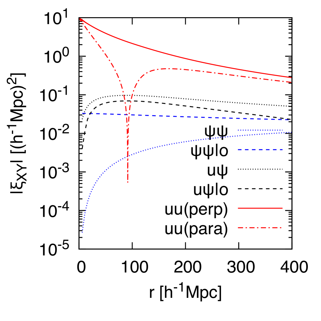
Figure 9: Left panel: Two-point correlations entering the covariance. The RSD contributions are in red, gravitational redshift contributions in blue, and cross correlations in black. Here $uu(\mathrm{perp})$ and $uu(\mathrm{para})$ are given by Eq. (85), $\psi\delta$ by Eq. (86), and $\psi\psi$ by Eq. (89). Note that $\psi\psi$ converges to a positive finite value at large separation, although this limit is very slowly reached (e.g. on the scale of the horizon). Correlations involving the local potential $\psi_{O}$ are indicated by $O$, e.g. $\psi\psi|O$ corresponds to $\langle(\psi_{1}-\psi_{O})\hskip 0.55496pt(\psi_{2}-\psi_{O})\rangle$. These types of correlations are not statistically homogeneous (depend not just on $r$), so we show only the angular average (monopole). Here we have taken $d=834\,h^{-1}\mathrm{Mpc}$, corresponding to redshift $z=0.3$. Right panel: Correlation function of the potential [Eq. (90)], broken down into its first three non-trivial multipoles, of which the main contribution is the monopole (shown also in left panel by the dashed blue curve). Here the multipoles are calculated for a patch of sky at a distance $\chi_{1}=\chi_{2}=834\,h^{-1}\mathrm{Mpc}$ (or $z=0.3$).

C.2 On the local potential

C.2.1 Impact on averages

The presence of the local potential $\psi_{O}$ in observables like $\psi-\psi_{O}$ requires a slight break from the usual way of thinking about cosmological averages. As mentioned earlier, the existence of the observer spoils statistical homogeneity by singling out one point for special treatment (the observer’s location). This is clear if we replace the ensemble average with a volume average, as allowed under ergodicity, for then averaging the local potential $\psi_{O}$ is equivalent to averaging over randomly placed observers, which is not justified; we make observations from a given point in space—and not any other point—meaning that when we perform an ensemble average of $\psi$ (or $\psi-\psi_{O}$) we should do so by averaging over only those configurations with $\psi(0)=\psi_{O}$ for given $\psi_{O}$ [91].

In principle we should replace the unconstrained two-point function (90) with the constrained one. In practice, however, we can usually get away with using the unconstrained one. This is because the effect of conditioning on $\psi_{O}$ is scale dependent, with impact weakening with distance from the observer, so that sufficiently far from the observer the constraint has little to no effect on correlations calculated in the usual way. For typical distances encountered in current surveys, the error we make in using the usual unconstrained average tends to be small, e.g. within the level of cosmic variance [91] (see also Ref. [96] in the context of weak lensing).

Incidentally, in the case $n_{s}<1$ and $\psi$ is Gaussian random, the constrained and unconstrained average is exactly equal:

$$\big{\langle}\big{(}\psi_{1}-\psi_{O}\big{)}\big{(}\psi_{2}-\psi_{O}\big{)}\,|\,O\big{\rangle}=\langle(\psi_{1}-\psi_{O})(\psi_{2}-\psi_{O})\big{\rangle}\,.$$ (96)

This can be shown by recalling a standard formula of conditional Gaussian statistics (see, e.g. Ref. [97], appendix D), namely, for $A,B,C$ Gaussian variables we have $\langle AB\,|\,C\rangle=\langle AB\rangle-\langle A\,|\,C\rangle\langle B\,|\,C\rangle/\langle C^{2}\rangle$. Applied to the potential,

$$\begin{split}\big{\langle}\big{(}\psi_{1}-\psi_{O}\big{)}\big{(}\psi_{2}-\psi_{O}\big{)}\,|\,O\big{\rangle}=\langle(\psi_{1}-\psi_{O})(\psi_{2}-\psi_{O})\big{\rangle}-\big{\langle}(\psi_{1}-\psi_{O})\hskip 0.59998pt\psi_{O}\big{\rangle}\hskip 0.59998pt\big{\langle}(\psi_{2}-\psi_{O})\hskip 0.59998pt\psi_{O}\big{\rangle}\hskip 0.89996pt\big{/}\hskip 0.89996pt\big{\langle}\psi^{2}_{O}\big{\rangle}\,.\end{split}$$ (97)

To show that the second term on the right-hand side vanishes, as Eq. (96) requires, we introduce an IR cut-off $k_{\mathrm{IR}}$ (which we send to zero at the end of the calculation) and replace $\langle\psi_{O}^{2}\rangle\equiv\sigma^{2}_{\psi}$ with $\sigma^{2}_{\psi}(k_{\mathrm{IR}})$ and $\tilde{\xi}_{\psi\psi}(r)$ with $\tilde{\xi}_{\psi\psi}(r;k_{\mathrm{IR}})$, i.e. we filter out power from scales $k<k_{\mathrm{IR}}$. Then since $\langle(\psi_{1}-\psi_{O})\hskip 0.59998pt\psi_{O}\rangle=\tilde{\xi}_{\psi\psi}(\chi_{1};k_{\mathrm{IR}})$ and $\langle(\psi_{2}-\psi_{O})\hskip 0.59998pt\psi_{O}\rangle=\tilde{\xi}_{\psi\psi}(\chi_{2};k_{\mathrm{IR}})$ we find for the second term

$$\big{\langle}(\psi_{1}-\psi_{O})\hskip 0.59998pt\psi_{O}\big{\rangle}\hskip 0.59998pt\big{\langle}(\psi_{2}-\psi_{O})\hskip 0.59998pt\psi_{O}\big{\rangle}\hskip 0.89996pt\big{/}\hskip 0.89996pt\big{\langle}\psi^{2}_{O}\big{\rangle}=\lim_{k_{\mathrm{IR}}\to 0}\,\tilde{\xi}_{\psi\psi}(\chi_{1};k_{\mathrm{IR}})\hskip 0.89996pt\tilde{\xi}_{\psi\psi}(\chi_{2};k_{\mathrm{IR}})\,\big{/}\,\sigma_{\psi}^{2}(k_{\mathrm{IR}})=0\,,$$

since in the limit $k_{\mathrm{IR}}\to 0$ the variance $\sigma_{\psi}^{2}(k_{\mathrm{IR}})\to\infty$, while $\tilde{\xi}_{\psi\psi}(r;k_{\mathrm{IR}})$ remains finite. These formal computations show that when integrating down to arbitrarily long modes ($k\to 0$) there is no impact from conditioning on the local potential and the average returns to its unconstrained form. Of course when dealing with a real survey modes larger than the survey cannot be measured and so the constrained and unconstrained averages will generally be different. But as mentioned, the effect of the constraint tends to be weak for all but the shallowest of surveys [96].

These results can be compared with those of Desjacques et al. [91] who have studied the issue of constrained averaging in Fourier space. Our results however have some differences with theirs, mainly because the power spectrum is no longer the Fourier transform of the correlation function so their results do not straightforwardly carry over to position space. In particular, estimating the power spectrum by the usual methods—i.e. spatial averaging of the constrained data assuming ergodicity—only converges to the unconstrained ensemble average in the limit of an infinite survey volume (corresponding to our taking $k_{\mathrm{IR}}\to 0$ above). Therefore in this case the constraint’s effect completely dies away. For finite volumes, while the impact of the constraint does not in general vanish, it is however small. For typical scales affected, such as those near the fundamental mode of the survey, the effect is within cosmic variance [91] (see also Ref. [96]).

C.2.2 Relation to the monopole

Since $\psi_{O}$ is not a local observable it is often neglected on the basis that, without any angular dependence, it is absorbed into the mean density, defined as the sky average. Indeed, $\psi_{O}$ is itself a monopole so will indeed drop out in the observed overdensity $\delta_{g}-\frac{1}{4\pi}\int\mathrm{d}^{2}{\hat{\mathbf{n}}}\,\delta_{g}$ (see Appendix D below). For instance, suppose $\psi(\chi\hat{\mathbf{n}})-\psi_{O}\subset\delta_{g}$. Clearly we have

$$\psi-\psi_{O}-\int\frac{\mathrm{d}^{2}\hat{\mathbf{n}}}{4\pi}\,(\psi-\psi_{O})=\psi-\int\frac{\mathrm{d}^{2}\hat{\mathbf{n}}}{4\pi}\,\psi\,.$$ (98)

In other words, there is no dependence on the local potential in the observed overdensity; the dependence on the local potential gets shuffled into the mean density. However, this is only the case when $\psi-\psi_{O}$ (or derivatives thereof) enters $\delta_{g}$ linearly, as in linear perturbation theory. In general, averaging and nonlinearity are not commutative operations, $\langle f(X)\rangle\neq f(\langle X\rangle)$ [98]. Therefore, in any model of $\delta_{g}-\frac{1}{4\pi}\int\mathrm{d}^{2}{\hat{\mathbf{n}}}\,\delta_{g}$ in which $\psi_{O}$ enters $\delta_{g}$ nonlinearly, it is important to retain such local terms, since at nonlinear order we can have products between terms evaluated at the source and terms evaluated at the observer [99]. This means that $\psi_{O}$ does not in general vanish upon monopole subtraction and so should not be neglected in, for example, Eq. (10). The correct approach is therefore to keep the local terms in the model, compute the monopole associated with the overdensity, and then subtract it from the model, as we discuss below in Appendix D.

These considerations of course concern full-sky coverage; for partial-sky coverage, even at linear order one cannot take for granted the absence of the local potential in the observed overdensity, as can be seen in Eq. (98) if one replaces $\psi-\psi_{O}$ with $W(\hat{\mathbf{n}})(\psi-\psi_{O})$.

Appendix D Full-sky correlations when the mean density is not known

Throughout this work we have routinely assumed that the mean background number density $\bar{n}_{g}$ is known, thus allowing us to isolate the ‘theoretical’ $\delta_{g}$ in the usual way, i.e. $\delta_{g}=(n_{g}-\bar{n}_{g})/\bar{n}_{g}$. But the mean number density is not known a priori and this leads to the ‘integral constraint’ [100, 101], the fact that since we measure the mean from the survey itself, whether it corresponds to the true mean or not, the overdensity is required by construction to average to zero over the survey. There is also the related issue that perturbations are not guaranteed to be observable quantities (e.g. the local potential) and what one deems the ‘background’ depends on choice of gauge (although note that these gauge effects are order $(\mathcal{H}/k)^{2}$ and so are suppressed with respect to the level of approximation used in this work).

These considerations are usually not a concern within the RSD paradigm. But with the inclusion of the (local) potential in the model one should take care to operationally define the galaxy overdensity from observable quantities. Furthermore, one also needs to be careful about what one means by ‘average’ in the absence of translation invariance in the wide-angle regime. Thus, for all-sky coverage over a wide redshift range we define the mean density as the sky average of the observed density, $\bar{n}_{g}\equiv\int_{\hat{\mathbf{n}}}n_{g}$, where as a shorthand $\int_{\hat{\mathbf{n}}}=\frac{1}{4\pi}\int\mathrm{d}^{2}\hat{\mathbf{n}}$ for the angular average. Then we extract (in redshift space) the overdensity $(n_{g}-\bar{n}_{g})/\bar{n}_{g}=(\delta_{g}-\int_{\hat{\mathbf{n}}}\delta_{g})/(1+\int_{\hat{\mathbf{n}}}\delta_{g})\simeq\delta_{g}-\int_{\hat{\mathbf{n}}}\delta_{g}$. That is, the observed fluctuation is the ‘theoretical’ one, $\delta_{g}$, with its monopole part removed [91, 102].

A short calculation shows that in going from $\delta_{g}\to\delta_{g}-\int_{\hat{\mathbf{n}}}\delta_{g}$ (linear or nonlinear $\delta_{g}$) the two-point function changes as

$$\xi^{(\mathrm{s})}(\chi_{1},\chi_{2},\cos\vartheta)\to\xi^{(\mathrm{s})}(\chi_{1},\chi_{2},\cos\vartheta)-C_{0}(\chi_{1},\chi_{2})/(4\pi)\,,$$ (99)

where $\xi^{(\mathrm{s})}(\chi_{1},\chi_{2},\cos\vartheta)$ is any rotationally-invariant correlation function (e.g. Eq. (4)), and we have recognised that because $\xi^{(\mathrm{s})}(\chi_{1},\chi_{2},\cos\vartheta)$ is rotationally invariant the average over the lines of sight $\hat{\mathbf{n}}_{1}$ and $\hat{\mathbf{n}}_{2}$ is equivalent to the average over the angular separation:

$$C_{0}(\chi_{1},\chi_{2})/(4\pi) =\int\frac{\mathrm{d}^{2}\hat{\mathbf{n}}_{1}}{4\pi}\int\frac{\mathrm{d}^{2}\hat{\mathbf{n}}_{2}}{4\pi}\,\xi^{(\mathrm{s})}(\chi_{1},\chi_{2},\cos\vartheta=\hat{\mathbf{n}}_{1}\cdot\hat{\mathbf{n}}_{2})=\frac{1}{2}\int^{1}_{-1}{\mathrm{d}\cos\vartheta}\,\xi^{(\mathrm{s})}(\chi_{1},\chi_{2},\cos\vartheta)\,,$$ (100)

which we have noted is just the definition of the monopole power $C_{0}$ (up to a factor of $4\pi$). Thus, the removal of the monopole in the overdensity translates to the removal of its monopole power $C_{0}$ in the two-point correlations. In other words, the harmonic series of the right-hand side of Eq. (99) in angular power $C_{\ell}$ begins non-trivially at $\ell=1$.

The question arises: does the subtraction of the monopole represent an important correction to the model (9)? For most surveys, no—the error made in neglecting the monopole should be small, with relative size $|C_{0}/(4\pi)\hskip 0.59998pt/\hskip 0.59998pt\xi^{(\mathrm{s})}|\ll 1$. For instance, at $z=0.3$ and $s=100\,h^{-1}\mathrm{Mpc}$ the correction is at the few-percent level. Qualitatively speaking, by changing to coordinates $s,d$, and $\mu$ we find that the relative correction grows with separation $s$, since the size of $\xi^{(\mathrm{s})}$ goes roughly as the inverse of $s$, while $C_{0}$ tends to be insensitive to $s$. In effect, for sufficiently large redshift (e.g. when we are justified in using the distant-observer approximation), $C_{0}$ acts as an overall shift and so does not change the shape of the correlation function (the position of the BAO peak is unaffected, for example [102]). In particular, only the $\ell=0$ multipole is shifted. On the other hand, at very low redshifts—for instance when the distant-observer limit breaks down and the curvature of the shells becomes relevant (over large $s$)—the monopole $C_{0}$ can induce in the multipoles a non-negligible scale-dependent shift. On the basis of symmetry we expect the leading-order wide-angle corrections are $\mathcal{O}(\epsilon^{2})$ for auto-correlations (in the mid-point parametrisation) and $\mathcal{O}(\epsilon)$ for cross-correlations.

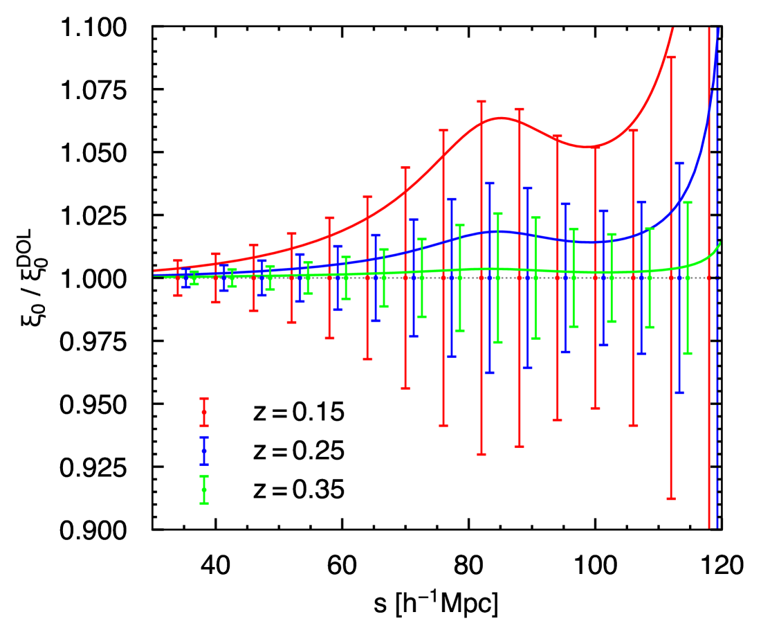
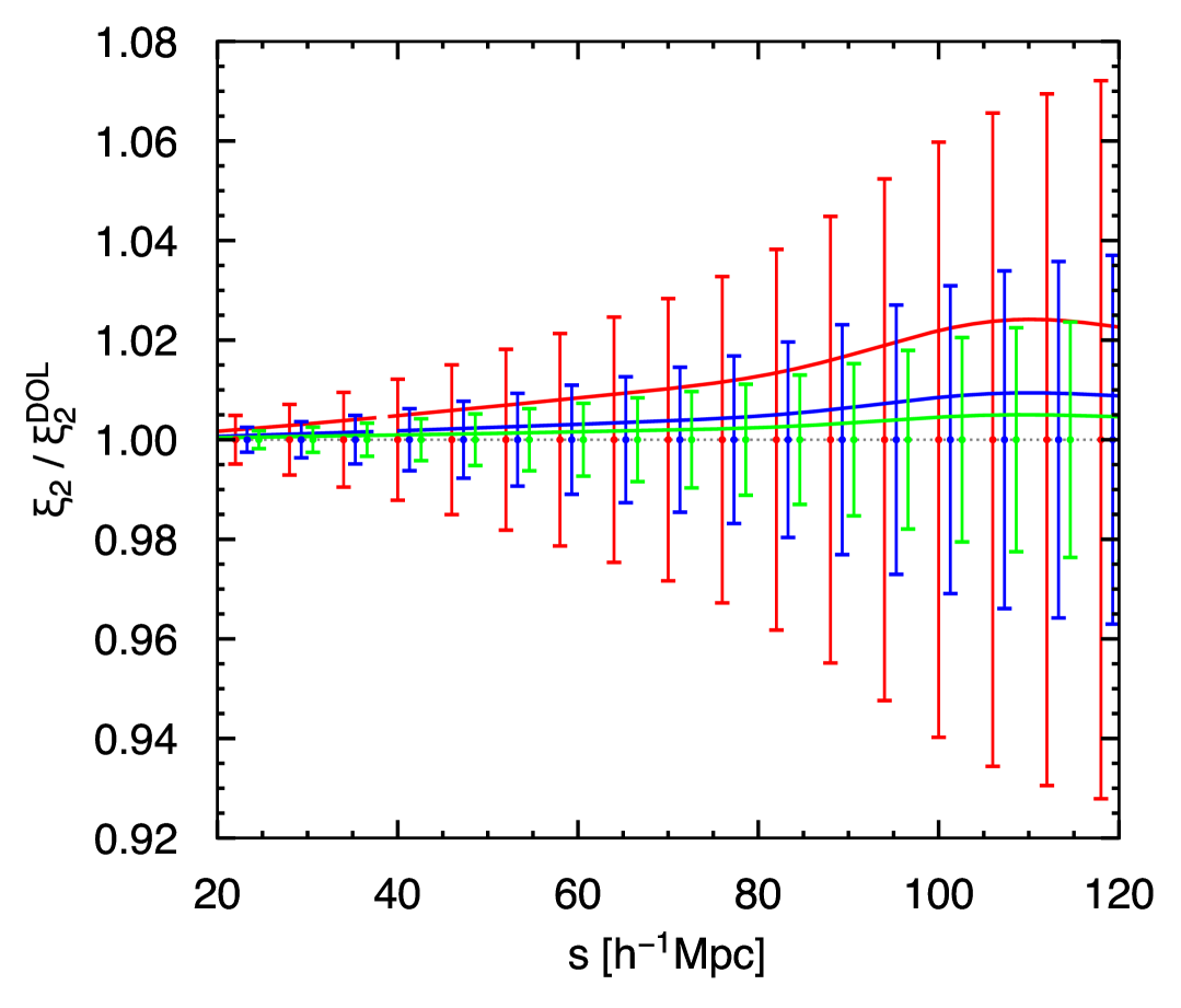
Figure 10: Forecasted uncertainties for BGS compared with the size of the wide-angle corrections defined as $\xi_{\ell}/\xi_{\ell}^{\mathrm{DOL}}$ (solid curves), with $\xi_{\ell}^{\mathrm{DOL}}$ given by the standard GSM [Eq. (36)] and $\xi_{\ell}$ the wide-angle generalisation [Eq. (9)]. Left panel shows monopole, right panel shows quadrupole. We use the fiducial BGS bias $b(z)=1.34/D(z)$, where $D(z)$ is the linear growth factor normalized so that $D(z=0)=1$ [103]. Here error bars (offset in the plot for clarity) are computed assuming DOL binned Gaussian covariances with bins of width $6\,h^{-1}\mathrm{Mpc}$.

Appendix E Impact of wide-angle effects on DESI BGS

Given the various novelties in the model (28), it is interesting to see in isolation just how important wide-angle effects are as a systematic compared to measurement uncertainties from upcoming surveys. Here we focus on the DESI Bright Galaxy Sample (BGS) [104], a low-redshift sample covering about a third of the sky ($f_{\mathrm{sky}}=0.339$) and where we might expect wide-angle corrections to be important. We show this comparison in Figure 10, ignoring all effects except the wide-angle ‘corrections’, which we recall are exact to all orders in $\epsilon=s/d$. Here it is seen that the monopole tends to be more affected than the quadrupole. This is not surprising given that the quadrupole is sourced by configurations with smaller opening angles than those of the monopole (see Section V.2). What is also clear is that the monopole at $z=0.15$ is significantly affected by wide-angle effects. However, we should caveat that the Gaussian covariances used to estimate the uncertainties are computed using the coffe code [105], which is limited to the distant-observer limit. Nevertheless, Ref. [106] found that in the case of the dipole the wide-angle corrections to the variance are negligible (due to cancellations).

Appendix F Calculation of $\llangle\Delta\psi\rrangle$ using the halo model

In this appendix we derive Eq. (45), i.e. the one- and two-halo contributions to the pairwise potential difference

$$\llangle\Delta\psi\rrangle\equiv\frac{\langle\hskip 0.59998ptn_{A}(\mathbf{x}_{1})\hskip 0.59998ptn_{B}(\mathbf{x}_{2})\hskip 0.59998pt\Delta\psi\rangle}{\langle n_{A}(\mathbf{x}_{1})\hskip 0.59998ptn_{B}(\mathbf{x}_{2})\rangle}$$ (101)

where $\Delta\psi=\psi(\mathbf{x}_{1})-\psi(\mathbf{x}_{2})$, $n_{A}(\mathbf{x}_{1})=\bar{n}_{A}[1+\delta_{A}(\mathbf{x}_{1})]$ and $n_{B}(\mathbf{x}_{2})=\bar{n}_{B}[1+\delta_{B}(\mathbf{x}_{2})]$ (assuming the usual density weighting). Note that the calculation of $\llangle\psi(\mathbf{x}_{1})-\psi_{O}\rrangle$ and $\llangle\psi(\mathbf{x}_{2})-\psi_{O}\rrangle$, as needed in $\bm{m}_{\mathrm{grav}}$, is essentially the same as the calculation of $\llangle\Delta\psi\rrangle$ we give below (with one minor difference which we point out at the end of this appendix).

Here we recall that the important aspect of this pairwise correlation is that it contains a nonvanishing one-point function, $\langle\psi(\mathbf{x}_{1})\hskip 0.59998pt\delta_{A}(\mathbf{x}_{1})\rangle$. As mentioned in the main text, this is because the gravitational redshift tends to trace overdense regions (i.e. potential wells), where $\langle\psi(\mathbf{x}_{1})\hskip 0.59998pt\delta_{A}(\mathbf{x}_{1})\rangle$ has a definite sign. By contrast, the analogous velocity statistic, $\llangle\Delta u\rrangle$, contains a vanishing one-point function since the mean velocity at a given point is zero (there are no preferred directions).

We carry out the calculation using the formalism of distributions [107], the basic quantity being the discrete distribution function

$$f_{d}(\mathbf{x},M,\tau)=\sum_{a}\delta_{\mathrm{D}}(\mathbf{x}-\mathbf{x}_{a}(\tau))\,\delta_{\mathrm{D}}(M-M_{a})\,,$$ (102)

where $M_{a}$ is the $a$th halo’s mass and $\mathbf{x}_{a}(\tau)$ is its (centre-of-mass) position at time $\tau$. The idea of the following calculation is to write Eq. (101) in terms of $f_{d}$ then use the known discrete statistics of $f_{d}$. We will not need to know the dynamics of $f_{d}$; only its statistics at a given time. We will henceforth suppress the time dependence.

Consider a population of dark matter haloes labelled $A$ in the mass range $M_{A1}\leq M\leq M_{A2}$. The number density is

$$n_{A}(\mathbf{x}) =\int^{M_{A2}}_{M_{A1}}\mathrm{d}M\,f_{d}(\mathbf{x},M)\,.$$ (103)

Making the standard assumption that all matter resides within haloes, each with characteristic profile $\rho(\mathbf{x};M)$ (e.g. the NFW profile), the matter density field $\rho_{\mathrm{tot}}(\mathbf{x})$ is obtained by convolving the point-particle distribution function with $\rho$, thereby turning the haloes into extended objects, i.e. we have

$$\rho_{\mathrm{tot}}(\mathbf{x}) =\int\mathrm{d}M\int\mathrm{d}^{3}\mathbf{y}\hskip 0.59998ptf_{d}(\mathbf{y},M)\hskip 0.89996pt\rho(\mathbf{x}-\mathbf{y};M)=\sum_{a}\rho(\mathbf{x}-\mathbf{x}_{a};M_{a})\,,$$ (104)

Here the integration is over all mass and we require $\int\mathrm{d}^{3}\mathbf{x}\,\rho(\mathbf{x};M)=M$ to ensure consistency with the predictions of perturbation theory on large scales [108]. With mass function $\mathrm{d}n/\mathrm{d}M=\langle f_{d}(\mathbf{x},M)\rangle$, the mean density is $\bar{\rho}=\langle\rho_{\mathrm{tot}}\rangle=\int\mathrm{d}M\hskip 0.59998ptM\hskip 0.59998pt({\mathrm{d}n}/{\mathrm{d}M})$.

By Poisson’s equation the potential sourced by fluctuations to the mean density $\langle\rho_{\mathrm{tot}}\rangle$ (rather than the density $\rho_{\mathrm{tot}}$ itself) can be written in position space as

$$\psi(\mathbf{x})=\lambda\hskip 0.59998ptG\int\mathrm{d}^{3}\mathbf{y}\,\frac{\rho_{\mathrm{tot}}(\mathbf{y})-\bar{\rho}}{|\mathbf{x}-\mathbf{y}|}\,.$$ (105)

Here $G$ is Newton’s constant of gravitation and we have defined $\lambda\equiv\mathcal{H}^{-1}a^{2}$. By linearity of Poisson’s equation, if $\rho_{\mathrm{tot}}(\mathbf{x})$ is a superposition of individual densities $\rho$, as it is in Eq. (104), then $\psi(\mathbf{x})$ is also a superposition of potentials given by

$$\phi(\mathbf{x};M) =\lambda G\int\mathrm{d}^{3}\mathbf{y}\,\frac{\rho(\mathbf{y};M)}{|\mathbf{x}-\mathbf{y}|}\,,$$ (106)

which individually solve Poisson’s equation with boundary condition $\phi\to 0$ as $\mathbf{x}\to\infty$. (Here we are assuming that haloes can be individually treated as isolated systems, i.e. with negligible tidal forces between them.) We have also dropped the integral over the mean field $\bar{\rho}$ since it gives an inconsequential normalisation constant which vanishes upon taking the difference of potentials (which is the quantity we are really after). The potential due to the entire distribution is then [cf. Eq. (104)]

$$\psi(\mathbf{x})=\int\mathrm{d}M\int\mathrm{d}^{3}\mathbf{y}\hskip 0.59998ptf_{d}(\mathbf{y},M)\hskip 0.89996pt\phi(\mathbf{x}-\mathbf{y};M)=\sum_{a}\phi(\mathbf{x}-\mathbf{x}_{a};M_{a})\,.$$ (107)

As with $\rho(\mathbf{x})$ above, the potential resulting from the entire distribution is given by the convolution of $f_{d}$ with the individual profiles $\phi$. But unlike $\rho$ the potential $\phi$, being a nonlocal function of $\rho$, reaches beyond the halo’s material extent (given, for instance, by the virial radius at which the profile is truncated). Therefore at any given point $\psi(\mathbf{x})$ can in principle receive contributions from many haloes, while that same point is located in one and only one halo (assuming halo exclusion). Note that in the case of a spherically symmetric profile, $\rho(\mathbf{x};M)=\rho(|\mathbf{x}|;M)$, Eq. (106) integrates to Eq. (32) in the main text.

To evaluate Eq. (101) we will need the first three $N$-point functions [109]:

$$\langle f_{d}(\mathbf{x}_{1},M_{1})\rangle \equiv\bar{f}_{1}={\mathrm{d}{n}}(M_{1})/{\mathrm{d}M}\,,$$ (108)

$$\langle f_{d}(\mathbf{x}_{1},M_{1})\hskip 0.89996ptf_{d}(\mathbf{x}_{2},M_{2})\rangle =\bar{f}_{1}\hskip 0.59998pt\delta_{\mathrm{D}}(\mathbf{x}_{1}-\mathbf{x}_{2})\hskip 0.89996pt\delta_{\mathrm{D}}(M_{1}-M_{2})+\bar{f}_{1}\bar{f}_{2}(1+\xi_{12})\,,$$ (109)

$$\langle f_{d}(\mathbf{x}_{1},M_{1})\hskip 0.89996ptf_{d}(\mathbf{x}_{2},M_{2})\hskip 0.89996ptf_{d}(\mathbf{x}_{3},M_{3})\rangle =\bar{f}_{1}\hskip 0.89996pt\delta_{\mathrm{D}}(\mathbf{x}_{1}-\mathbf{x}_{2})\hskip 0.89996pt\delta_{\mathrm{D}}(M_{1}-M_{2})\hskip 0.89996pt\delta_{\mathrm{D}}(\mathbf{x}_{1}-\mathbf{x}_{3})\hskip 0.89996pt\delta_{\mathrm{D}}(M_{1}-M_{3})$$

$$\quad+\bar{f}_{1}\hskip 0.89996pt\bar{f}_{3}\hskip 0.59998pt(1+\xi_{13})\hskip 0.89996pt\delta_{\mathrm{D}}(\mathbf{x}_{1}-\mathbf{x}_{2})\hskip 0.89996pt\delta_{\mathrm{D}}(M_{1}-M_{2})+\text{2 cyc.}$$

$$\quad+\bar{f}_{1}\hskip 0.59998pt\bar{f}_{2}\hskip 0.59998pt\bar{f}_{3}\hskip 0.59998pt(1+\xi_{12}+\text{2 cyc.})\,,$$ (110)

where $\xi_{ij}\equiv\xi_{hh}(\mathbf{x}_{i}-\mathbf{x}_{j},M_{i},M_{j})$, $i,j=1,2,3$, is the cross-correlation function between haloes of mass $M_{i}$ and $M_{j}$. In this work we take $\xi(\mathbf{r},M_{A},M)=b_{1}(M_{A})\hskip 0.59998ptb_{1}(M)\hskip 0.59998pt\xi_{mm}(r)$, with linear bias $b_{1}(M_{A})$ determined by the peak–background split and $\xi_{m}(r)$ the matter correlation function. Here we have assumed Poisson noise and that the clustering is Gaussian so that we can ignore the connected three-point function that would otherwise be present in the last line of Eq. (110). Note that the structure of $\langle f_{d}(1)\hskip 0.89996ptf_{d}(2)\hskip 0.89996ptf_{d}(3)\rangle$, for instance, is that we can have (i) all three points in a single halo (one-halo term; first line in Eq. (110)), (ii) two points in one halo and one point in a separate halo (two-halo term; second-to-last line), or (iii) each of the three points in distinct haloes (three-halo term; last line).

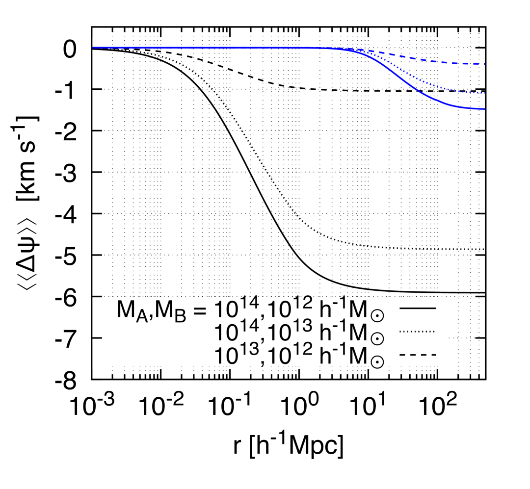
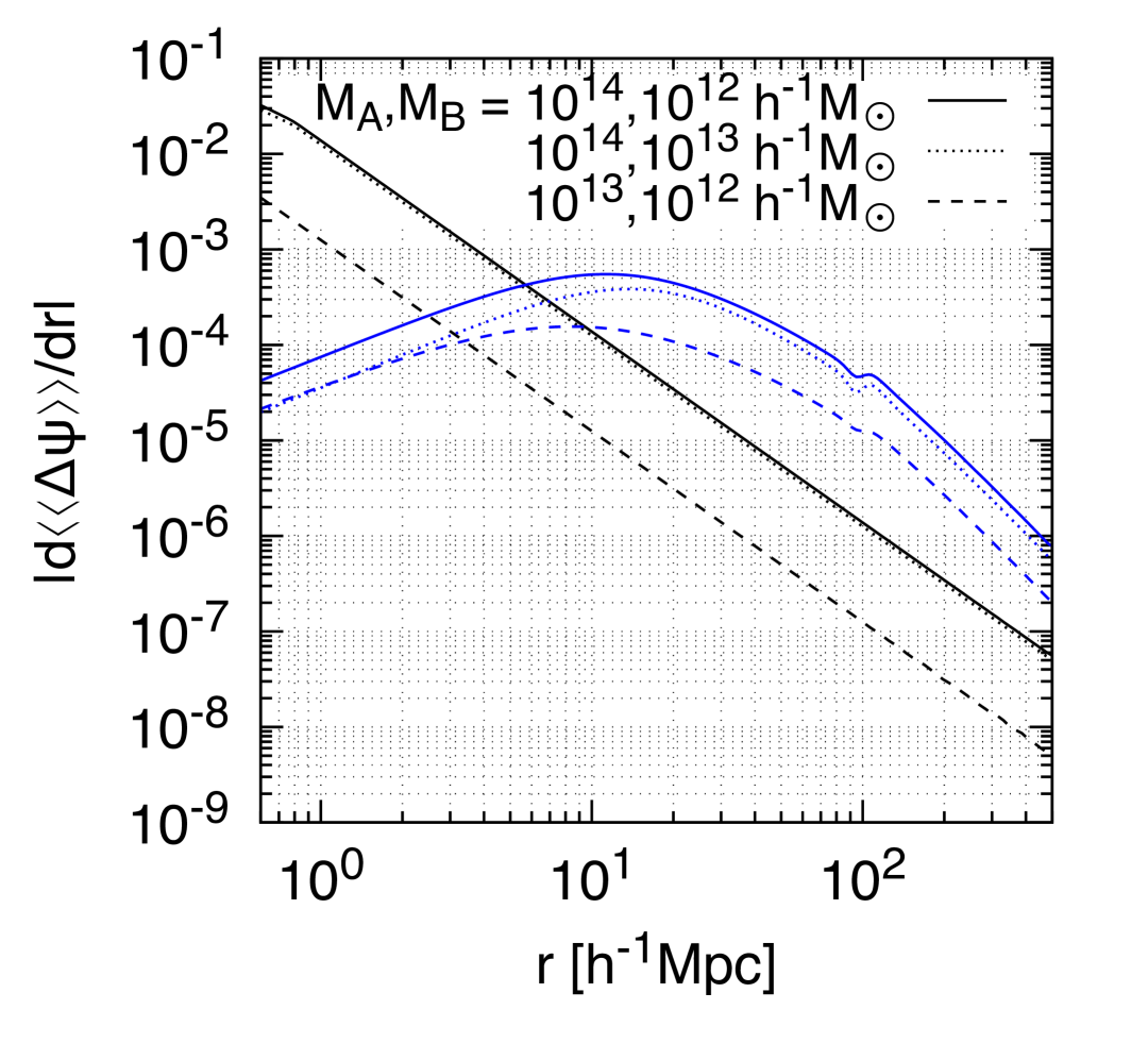
Figure 11: Left panel: Contributions to $\llangle\Delta\psi\rrangle$ from the one-halo (black curves) and two-halo (blue curves) terms for three different mass combinations. (Here $\llangle\Delta\psi\rrangle$ is multiplied by $-\mathcal{H}$; the units are thus $\mathrm{km}\,\mathrm{s}^{-1}$.) Note that the linear prediction of $\llangle\Delta\psi\rrangle$ is virtually identical to the two-halo curves. Note also that this plot is essentially Figure 6 but here on a linear scale to show more clearly the relative size. Right panel: The corresponding derivatives of each curve in the left panel [the form in which $\llangle\Delta\psi\rrangle$ enters the multipoles at first order]. Here $z=0.3$ and we assume a truncated NFW profile with concentration $c=9$.

For simplicity we consider two narrow, non-overlapping mass bins of width $\delta M_{A}$ and $\delta M_{B}$, centred at $M=M_{A}$ and $M=M_{B}$, respectively. By Eq. (103) we then have $n_{A}(\mathbf{x}_{1})\approx\delta M_{A}\hskip 0.89996ptf_{d}(\mathbf{x}_{1},M_{A})$ and $n_{B}(\mathbf{x}_{2})\approx\delta M_{B}\hskip 0.89996ptf_{d}(\mathbf{x}_{2},M_{B})$. The denominator of Eq. (101) is given by the standard result:

$$\langle n_{A}(\mathbf{x}_{1})\hskip 0.59998ptn_{B}(\mathbf{x}_{2})\rangle =\bar{n}_{A}\hskip 0.59998pt\bar{n}_{B}\left(1+\xi_{AB}(\mathbf{x}_{1}-\mathbf{x}_{2})+\frac{\delta_{AB}}{\bar{n}_{A}}\hskip 0.59998pt\delta_{\mathrm{D}}(\mathbf{x}_{1}-\mathbf{x}_{2})\right)\,,$$

where $\bar{n}_{A}\approx\delta M_{A}\langle f_{d}(\mathbf{x},M_{A})\rangle=\delta M_{A}\hskip 0.59998pt\mathrm{d}n(M_{A})/\mathrm{d}M$ and $\bar{n}_{B}\approx\delta M_{B}\langle f_{d}(\mathbf{x},M_{B})\rangle=\delta M_{B}\hskip 0.59998pt\mathrm{d}n(M_{B})/\mathrm{d}M$ are the mean number densities.

The novel part of the calculation is the evaluation of the numerator of Eq. (101). In terms of the distribution function it reads

$$\langle n_{A}(\mathbf{x}_{1})\hskip 0.59998ptn_{B}(\mathbf{x}_{2})\hskip 0.59998pt\Delta\psi\rangle=\delta M_{A}\hskip 0.59998pt\delta M_{B}\!\int\mathrm{d}M\!\int\mathrm{d}^{3}\mathbf{x}\,\Big{\{}\big{\langle}f_{d}(\mathbf{x}_{1},M_{A})\hskip 0.59998ptf_{d}(\mathbf{x}_{2},M_{B})\hskip 0.59998ptf_{d}(\mathbf{x},M)\big{\rangle}\big{[}\phi(\mathbf{x}_{1}-\mathbf{x};M)-\phi(\mathbf{x}_{2}-\mathbf{x};M)\big{]}\Big{\}}\,.$$

Substituting the three-point function (110) yields several terms in the integrand. The (unintegrated) one-halo term [first line in Eq. (110)] is proportional to $\delta_{\mathrm{D}}(\mathbf{x}_{1}-\mathbf{x}_{2})$ so vanishes at nonzero separation, while the integrated three-halo terms yields the clustering contribution. The remaining terms in Eq. (110), the integrated two-halo terms, yield the one-halo term which, after some algebra, can be written as [with $M_{1}\equiv M_{A}$, $M_{2}\equiv M_{B}$]

$$\begin{split}&\langle n_{A}(\mathbf{x}_{1})\hskip 0.59998ptn_{B}(\mathbf{x}_{2})\hskip 0.59998pt\Delta\psi\rangle=\bar{n}_{A}\hskip 0.89996pt\bar{n}_{B}\hskip 0.59998pt[1+\xi_{AB}(\mathbf{x}_{1}-\mathbf{x}_{2})]\\ &\qquad\quad\times\int\mathrm{d}M\int\mathrm{d}^{3}\mathbf{x}\,\Big{\{}\big{[}\delta_{\mathrm{D}}(\mathbf{x}_{1}-\mathbf{x})\hskip 0.89996pt\delta_{\mathrm{D}}(M_{1}-M)+(1\leftrightarrow 2)\big{]}\big{[}\phi(\mathbf{x}_{1}-\mathbf{x};M)-\phi(\mathbf{x}_{2}-\mathbf{x};M)\big{]}\Big{\}}+\text{2-halo terms}\,.\end{split}$$ (111)

In arriving at this expression we have used that one of the three two-halo permutations is symmetric in $(\mathbf{x}_{1},M_{1})$ and $(\mathbf{x}_{2},M_{2})$ so therefore vanishes upon integration against the potential difference, which is anti-symmetric in $\mathbf{x}_{1}$ and $\mathbf{x}_{2}$. (In any case it vanishes at nonzero separation because of the delta function $\delta_{\mathrm{D}}(\mathbf{x}_{1}-\mathbf{x}_{2})$.) Integrating the foregoing expression is trivial and gives

$$\begin{split}&\langle n_{A}(\mathbf{x}_{1})\hskip 0.59998ptn_{B}(\mathbf{x}_{2})\hskip 0.59998pt\Delta\psi\rangle=\bar{n}_{A}\hskip 0.89996pt\bar{n}_{B}\hskip 0.59998pt\big{[}1+\xi_{AB}(\mathbf{x}_{1}-\mathbf{x}_{2})\big{]}\big{[}\phi_{A}(0)-\phi_{A}(\mathbf{x}_{2}-\mathbf{x}_{1})+\phi_{B}(\mathbf{x}_{1}-\mathbf{x}_{2})-\phi_{B}(0)\big{]}+\text{2-halo terms}\,,\end{split}$$

where $\phi_{A}(\mathbf{x})\equiv\phi(\mathbf{x};M_{A})$ and $\phi_{B}(\mathbf{x})\equiv\phi(\mathbf{x};M_{B})$. Dividing by the normalisation $\langle n_{A}(\mathbf{x}_{1})\hskip 0.59998ptn_{B}(\mathbf{x}_{2})\rangle=\bar{n}_{A}\hskip 0.89996pt\bar{n}_{B}\hskip 0.59998pt[1+\xi_{AB}(\mathbf{x}_{1}-\mathbf{x}_{2})]$, $\mathbf{x}_{1}\neq\mathbf{x}_{2}$, and writing $\llangle\Delta\psi\rrangle=\llangle\Delta\psi\rrangle_{\text{1h}}+\llangle\Delta\psi\rrangle_{\text{2h}}$, we arrive at the main result:

$$\llangle\Delta\psi\rrangle_{\text{1h}}=[\phi_{A}(0)-\phi_{A}(\mathbf{x}_{2}-\mathbf{x}_{1})]-[\phi_{B}(0)-\phi_{B}(\mathbf{x}_{1}-\mathbf{x}_{2})]\,.$$ (112)

This equation reduces to Eq. (46) in the case of spherical symmetry, $\phi_{A}(r)\equiv\phi_{A}(\mathbf{x}_{2}-\mathbf{x}_{1})$ and $\phi_{B}(r)\equiv\phi_{B}(\mathbf{x}_{1}-\mathbf{x}_{2})$ with $r=|\mathbf{x}_{1}-\mathbf{x}_{2}|$. Notice that Eq. (112) is not simply the potential difference $\phi_{B}(r)-\phi_{A}(r)$, but the difference of potentials, normalised to their respective central values. This ensures that $\llangle\Delta\psi\rrangle_{\mathrm{1h}}=0$ at $r=0$ (which we should have on account of anti-symmetry). Note that the one-halo term does not depend on the correlation function $\xi_{AB}$ (the normalisation completely drops out).

Obtaining the clustering contribution (two-halo term) is a more straightforward affair. From the last line of terms in Eq. (110),

$$\llangle\Delta\psi\rrangle_{\text{2h}}=\frac{1}{1+\xi_{AB}(r)}\,\Big{\{}[\xi_{\psi\delta_{A}}(0)-\xi_{\psi\delta_{A}}(r)]-[\xi_{\psi\delta_{B}}(0)-\xi_{\psi\delta_{B}}(r)]\Big{\}}\,,$$ (113)

where $\xi_{\psi\delta_{A}}(r)$ is given by Eq. (34). A similar expression holds for $\xi_{\psi\delta_{B}}(r)$ [take $M_{A}\to M$ and $M\to M_{B}$]. Note that the integration over $\mathbf{x}$ is a convolution of each halo with its associated potential $\phi$, while the integration over $M$ is over all mass since the potential is sourced by all matter (not just the matter belonging to the population of tracer $A$).

Now, as the one-halo term shares the same basic form as the two-halo term we can therefore write

$$\llangle\Delta\psi\rrangle =\llangle\Delta\psi\rrangle_{\text{1h}}+\llangle\Delta\psi\rrangle_{\text{2h}}$$

$$\simeq[\xi_{\psi\delta_{A}}(0)+\phi_{A}(0)-\xi_{\psi\delta_{A}}(r)-\phi_{A}(r)]-[\xi_{\psi\delta_{B}}(0)+\phi_{B}(0)-\xi_{\psi\delta_{B}}(r)-\phi_{B}(r)]\,,$$ (114)

where we have dropped the normalisation in the second line. The last line says that the clustering contributions, $\xi_{\psi\delta_{A}}$ and $\xi_{\psi\delta_{B}}$, are augmented by a halo correction, $\phi_{A}$ and $\phi_{B}$, for both zero-lag terms and scale-dependent terms. At the field level we heuristically think of these corrections as coming from the individual $\phi$’s superposed on the large-scale linear potential, having the effect of deepening the potential at the sites of tracers (where light is emitted).

The left panel of Figure 11 shows the one- and two-halo contributions to $\llangle\Delta\psi\rrangle$, while the right panel shows the derivatives thereof. The first-order contribution to the multipoles comes from the derivative while at second order we can have products containing $\llangle\Delta\psi\rrangle$ (not differentiated). The point here is that at first order the two-halo term is more important than the one-halo term (for $r\gtrsim 10\,h^{-1}\mathrm{Mpc}$). While at second order it is the one-halo term which is more important (on all scales in fact) due to its larger one-point function. For two of the mass combinations (solid and dotted curves) the difference between $\llangle\Delta\psi\rrangle_{\mathrm{1h}}$ and $\llangle\Delta\psi\rrangle_{\mathrm{2h}}$ is significant. For instance, for $M_{A}=10^{14}h^{-1}M_{\odot}$ and $M_{B}=10^{12}h^{-1}M_{\odot}$ at $r=20\,h^{-1}\mathrm{Mpc}$ we have that $\llangle\Delta\psi\rrangle_{\mathrm{1h}}$ is about an order of magnitude larger than the term $\llangle\Delta\psi\rrangle_{\mathrm{2h}}$ (which we find is very similar to the estimate of linear theory, e.g. by writing $\xi_{\psi\delta_{A}}(0)=b_{1}(M_{A})\hskip 0.59998pt\xi_{\psi\delta}(0)$ and evaluating $\xi_{\psi\delta}(0)$ using Eq. (86)). The other mass combination yields a smaller one-halo contribution, albeit one which is still a factor of two larger that the corresponding two-halo contribution (the total contribution is a factor of three larger than the two-halo term).

Finally, let us give here the formula for $\llangle\psi(\mathbf{x}_{1})-\psi_{O}\rrangle_{\mathrm{1h}}$ and $\llangle\psi(\mathbf{x}_{2})-\psi_{O}\rrangle_{\mathrm{1h}}$. As mentioned at the start of this section, the calculation presented above goes through in much the same way for these two statistics. Returning to Eq. (111) but putting $\phi(\mathbf{x}_{1}-\mathbf{x};M)-\phi(\mathbf{x}_{2}-\mathbf{x};M)\to\phi(\mathbf{x}_{1}-\mathbf{x};M)-\phi(-\mathbf{x};M)$ for the first statistic and $\phi(\mathbf{x}_{1}-\mathbf{x};M)-\phi(\mathbf{x}_{2}-\mathbf{x};M)\to\phi(\mathbf{x}_{2}-\mathbf{x};M)-\phi(-\mathbf{x};M)$ for the second, then repeating many of the same steps above, we find

$$\llangle\psi(\mathbf{x}_{1})-\psi_{O}\rrangle_{\mathrm{1h}} =[\phi_{A}(0)-\phi_{A}(-\mathbf{x}_{1})]-[\phi_{B}(-\mathbf{x}_{2})-\phi_{B}(\mathbf{x}_{1}-\mathbf{x}_{2})]\,,$$ (115)

$$\llangle\psi(\mathbf{x}_{2})-\psi_{O}\rrangle_{\mathrm{1h}} =[\phi_{B}(0)-\phi_{B}(-\mathbf{x}_{2})]-[\phi_{A}(-\mathbf{x}_{1})-\phi_{A}(\mathbf{x}_{2}-\mathbf{x}_{1})]\,,$$ (116)

for $\mathbf{x}_{1}\neq\mathbf{x}_{2}$. In the case of spherical symmetry, $\phi_{A}(-\mathbf{x}_{1})=\phi_{A}(\chi_{1}^{\prime})$ and $\phi_{B}(-\mathbf{x}_{2})=\phi_{B}(\chi_{2}^{\prime})$. Note the difference of Eq. (115) and Eq. (116) is Eq. (112) (terms depending on radial distances cancel). Note also that compared with Eq. (112) there is in fact an additional term on the right-hand sides of Eqs. (115) and (116); this traces back to the first term in the second line of Eq. (110) (which is not identically zero anymore). However, this term is proportional to $\delta_{\mathrm{D}}(\mathbf{x}_{1}-\mathbf{x}_{2})$, i.e. a shot noise contribution, so can be ignored if $\mathbf{x}_{1}\neq\mathbf{x}_{2}$, as we have done above.

Appendix G Configuration-space formula for the dipole induced by RSD in the wide-angle regime

In the course of the calculations of Section VII we gave a neat expression for the leading-order RSD dipole in terms of the pairwise mean velocity. In the mid-point parametrisation it reads (see Eq. (64) in the main text)

$$\xi_{1}^{\mathrm{RSD}}(s,d)=-\epsilon\hskip 0.59998pt\frac{4}{5s^{4}}\frac{\mathrm{d}}{\mathrm{d}s}\big{(}s^{4}\llangle\bar{u}\rrangle\big{)}+\mathcal{O}(\epsilon^{2})=-\epsilon\hskip 0.59998pt\frac{4}{5}\left(\frac{4}{s}\llangle\bar{u}\rrangle+\frac{\mathrm{d}\llangle\bar{u}\rrangle}{\mathrm{d}s}\right)+\mathcal{O}(\epsilon^{2})\,,$$ (117)

where the first term in the second equality is due to the radial volume effect while the second term is due to the projection of distinct lines of sight onto the mid-point. Here we confirm that this is indeed equivalent to the more standard expression of the RSD dipole (see, e.g. Ref. [60], equation 61)

$$\begin{split}\xi_{1}^{\mathrm{RSD}}(s,d)&=-\epsilon(b_{A}-b_{B})\hskip 0.59998ptf\int\frac{k^{2}\mathrm{d}k}{2\pi^{2}}\left(2\hskip 0.59998pt\frac{j_{1}(ks)}{ks}-\frac{2}{5}j_{2}(ks)\right)P_{\delta\delta}(k)+\mathcal{O}(\epsilon^{2})\,.\end{split}$$ (118)

That these two equations are equivalent can be verified by: substituting into Eq. (117) the linear expression $\llangle\bar{u}\rrangle(s)\simeq-(1/2)(b_{A}-b_{B})\hskip 0.89996pt\xi_{u\hskip 0.49164pt\delta}(s)$, with $\xi_{u\hskip 0.49164pt\delta}$ replaced by its Fourier representation (83); evaluating the derivative with respect to $s$; and using that $\mathrm{d}j_{1}(x)/\mathrm{d}x=j_{1}(x)/x-j_{2}(x)$. Formula (117) reaffirms that pairwise functions (and derivatives thereof) form the basic building blocks of all multipoles, whether in the distant-observer limit or in the wide-angle regime. Moreover, Eq. (117), such as it is written, has the advantage that it does not explicitly depend on the modelling details of $\llangle\bar{u}\rrangle$ (dynamics and bias), unlike Eq. (118).

Note that when cross-checking expressions of odd multipoles one may find an overall sign difference. This is due to the convention being used for the separation vector: either $\mathbf{s}=\mathbf{s}_{1}-\mathbf{s}_{2}$ (used here) or $\mathbf{s}=\mathbf{s}_{2}-\mathbf{s}_{1}$. (This convention should not be confused with the line-of-sight convention.) No such ambiguity exists for the even multipoles since these are even functions of $\mu=\hat{\mathbf{s}}\cdot\hat{\mathbf{n}}$. For numerical work we multiply our dipole by $-1$, in keeping with the convention used in the simulation measurements (opposite our own).

Appendix H Anti-symmetric part of the cross-correlation function up to second order in Gaussian cumulants

For completeness, we give here the expression for the anti-symmetric part of the cross-correlation function up to second order:

$$\begin{split}\xi^{(\mathrm{s})}_{[AB]}&=\xi_{[AB]}-\partial_{a}\hskip 0.59998ptm^{a}_{[AB]}+\tfrac{1}{2}\partial_{a}\partial_{b}C^{ab}_{[AB]}+\partial_{a}\partial_{b}\hskip 0.59998pt(m^{a}_{[AB]}\hskip 0.59998ptm^{b}_{(AB)})-m^{a}_{[AB]}\hskip 0.59998pt\partial_{a}\hskip 0.59998pt\xi_{(AB)}-m^{a}_{(AB)}\hskip 0.59998pt\partial_{a}\hskip 0.59998pt\xi_{[AB]}\\ &\quad-\xi_{(AB)}\hskip 0.59998pt\partial_{a}\hskip 0.59998ptm^{a}_{[AB]}-\xi_{[AB]}\hskip 0.59998pt\partial_{a}\hskip 0.59998ptm^{a}_{(AB)}+\tfrac{1}{2}C^{ab}_{(AB)}\hskip 0.59998pt\partial_{a}\partial_{b}\hskip 0.59998pt\xi_{[AB]}+\tfrac{1}{2}C^{ab}_{[AB]}\hskip 0.59998pt\partial_{a}\partial_{b}\hskip 0.59998pt\xi_{(AB)}\\ &\quad+\tfrac{1}{2}\xi_{(AB)}\hskip 0.89996pt\partial_{a}\hskip 0.59998pt\partial_{b}C^{ab}_{[AB]}+\tfrac{1}{2}\xi_{[AB]}\hskip 0.89996pt\partial_{a}\hskip 0.59998pt\partial_{b}C^{ab}_{(AB)}+\partial_{a}\hskip 0.59998pt\xi_{[AB]}\hskip 0.59998pt\partial_{b}C^{ab}_{(AB)}+\partial_{a}\hskip 0.59998pt\xi_{(AB)}\hskip 0.59998pt\partial_{b}C^{ab}_{[AB]}\,,\end{split}$$ (119)

where repeated lowercase letters $a,b=1,2,\ldots,6$ are summed over (no sum over labels $A$, $B$), all quantities are evaluated at $\mathbf{S}=(\mathbf{s}_{1},\mathbf{s}_{2})$, and we recall $\partial_{a}=\partial/\partial\hskip 0.59998ptS^{a}$ is the partial derivative on six-dimensional Cartesian space. (Note that $A$ and $B$ are not tensorial indices but rather labels we find convenient to use to distinguish between symmetric and anti-symmetric parts.) This expression, valid for both radial and transverse distortions, follows from Eq. (60) by inserting into it $\xi_{AB}=\xi_{(AB)}+\xi_{[AB]}$, $m^{a}_{AB}=m^{a}_{(AB)}+m^{a}_{[AB]}$, and $C^{ab}_{AB}=C^{ab}_{(AB)}+C^{ab}_{[AB]}$, and remembering that the product here of a symmetric and anti-symmetric part is overall anti-symmetric, hence the large number of cross terms. Except for the first three terms, all terms in Eq. (119) are quadratic in correlators.

Now if we assume no lightcone effect, $\xi_{[AB]}=0$ (see Eq. (27)). If we keep only the leading contribution to the cumulants, $C_{[AB]}=0$ (but $m_{[AB]}\neq 0$). Under these two approximations Eq. (119) is greatly simplified and we are left with

$$\xi^{(\mathrm{s})}_{[AB]} \simeq-\partial_{a}\hskip 0.59998ptm^{a}_{[AB]}-m^{a}_{[AB]}\hskip 0.59998pt\partial_{a}\hskip 0.59998pt\xi_{(AB)}-\xi_{(AB)}\hskip 0.59998pt\partial_{a}\hskip 0.59998ptm^{a}_{[AB]}+\partial_{a}\partial_{b}\hskip 0.59998pt(m^{a}_{[AB]}\hskip 0.59998ptm^{b}_{(AB)})$$

$$=-\partial_{a}\big{[}(1+\xi_{(AB)})\,m_{[AB]}^{a}\big{]}+\partial_{a}\partial_{b}\hskip 0.59998pt(m^{a}_{[AB]}\hskip 0.59998ptm^{b}_{(AB)})\,.$$ (120)

Except for the last term, this is Eq. (60) in the main text.

The last term is the disconnected piece of the second moment which is often neglected in streaming models (as we have done in Section VII). Since this is the only term in the expression which contains a double derivative, developing it requires some work. First, distributing the derivatives:

$$\partial_{a}\partial_{b}\hskip 0.59998pt(m^{a}_{[AB]}\hskip 0.59998ptm^{b}_{(AB)}) =\partial_{a}\partial_{b}m^{a}_{[AB]}\hskip 0.59998ptm^{b}_{(AB)}+m^{a}_{[AB]}\hskip 0.59998pt\partial_{a}\partial_{b}m^{b}_{(AB)}+\partial_{a}m^{a}_{[AB]}\hskip 0.59998pt\partial_{b}m^{b}_{(AB)}+\partial_{b}m^{a}_{[AB]}\hskip 0.59998pt\partial_{a}m^{b}_{(AB)}$$

$$=m_{(AB)}\cdot\partial\,(\partial\cdot m_{[AB]})+m_{[AB]}\cdot\partial\,(\partial\cdot m_{(AB)})+(\partial\cdot m_{[AB]})\hskip 0.59998pt(\partial\cdot m_{(AB)})+\partial_{b}m^{a}_{[AB]}\hskip 0.59998pt\partial_{a}m^{b}_{(AB)}$$

where in the second line we have used that $\partial_{a}\partial_{b}=\partial_{b}\partial_{a}$.

In our perturbative scheme recall that we count as the same order terms suppressed by $\mathcal{H}/k$ and terms suppressed by $\epsilon$, i.e. $\mathcal{H}/k\sim\epsilon$. Note that $m^{\mathrm{grav}}_{[AB]}\sim m^{\mathrm{RSD}}_{[AB]}\sim\epsilon\hskip 0.89996ptm^{\mathrm{RSD}}_{(AB)}$. We have the following divergences:

$$\partial\cdot m_{[AB]}^{\mathrm{grav}} =\mu\frac{\mathrm{d}\llangle\Delta\psi\rrangle}{\mathrm{d}s}+\mathcal{O}(\epsilon\cdot\mathcal{H}/k)\,,$$ (121)

$$\partial\cdot m_{(AB)}^{\mathrm{RSD}} =\mu^{2}\frac{\mathrm{d}\llangle\Delta{u}\rrangle}{\mathrm{d}s}+\mathcal{O}(\epsilon^{2})\,,$$ (122)

$$\partial\cdot m_{[AB]}^{\mathrm{RSD}} =\epsilon\hskip 0.59998pt\mu(1-\mu^{2})\frac{\mathrm{d}\llangle\bar{u}\rrangle}{\mathrm{d}s}+\mathcal{O}(\epsilon^{2})\,,$$ (123)

where here we only need to compute the wide-angle effect for the anti-symmetric part of RSD.

Appendix I Coordinate relations and other useful formulae

This mathematical appendix gathers together some useful formulae relating spherical coordinates $\chi_{1},\chi_{2},\cos\vartheta$ (in which correlations on the full sky are naturally described) to the standard coordinates $s,d,\mu$ (in which the multipoles are defined). These formulae are needed in the calculations of Section VII but more generally in situations where one wishes to calculate multipoles in the absence of translation invariance.

First note $\chi_{1}=|\mathbf{s}_{1}|$, $\chi_{2}=|\mathbf{s}_{2}|$, $s\equiv|\mathbf{s}_{1}-\mathbf{s}_{2}|$, while $d=|\mathbf{d}|$ and $\mu=\hat{\mathbf{s}}\cdot\hat{\mathbf{n}}$ depend on the choice of $\mathbf{d}$ and $\hat{\mathbf{n}}$; here they are specified according to the mid-point prescription, in which $\mathbf{d}\equiv(\mathbf{s}_{1}+\mathbf{s}_{2})/2$ and $\hat{\mathbf{n}}\equiv\hat{\mathbf{d}}$. The coordinate relations are

$$s =\big{(}\chi_{1}^{2}+\chi_{2}^{2}-2\chi_{1}\chi_{2}\cos\vartheta\big{)}^{1/2}\,,$$ (124a)

$$d =\tfrac{1}{2}\big{(}\chi_{1}^{2}+\chi_{2}^{2}+2\chi_{1}\chi_{2}\cos\vartheta\big{)}^{1/2}\,,$$ (124b)

$$\mu =\frac{\chi_{1}^{2}-\chi_{2}^{2}}{[(\chi_{1}^{2}+\chi_{2}^{2})^{2}-(2\chi_{1}\chi_{2}\cos\vartheta)^{2}]^{1/2}}\,,$$ (124c)

where we recall $\cos\vartheta=\hat{\mathbf{n}}_{1}\cdot\hat{\mathbf{n}}_{2}$. These relations all follow from straightforward applications of the cosine rule, with analogous relations in real space [replace $\mu$ by $\mu^{\prime}$, $s$ by $r$, $\chi_{1}$ by $\chi_{1}^{\prime}$, $\chi_{2}$ by $\chi_{2}^{\prime}$, etc]. Note that $s$ and $d$ are positive valued; $\mu<0$ when $\chi_{1}<\chi_{2}$; and $\mu>0$ when $\chi_{1}>\chi_{2}$. Under pair exchange $(\mathbf{s}_{1}\leftrightarrow\mathbf{s}_{2}$) we have $\mu\to-\mu$ and $\chi_{1}\leftrightarrow\chi_{2}$. Note also that the relation between coordinates is unique since the jacobian is ${2\chi_{1}^{2}\chi_{2}^{2}}/{s^{2}d^{2}}$, which is nonzero for all physical configurations (i.e. excluding the unphysical case in which one or both points are at the origin, see Figure 1).

An important regime which can be treated perturbatively concerns small opening angles, $\epsilon\equiv s/d\ll 1$. In this more restricted wide-angle regime we can linearize about the distant-observer limit ($\epsilon=0$). The radial distances to linear order in $\epsilon$ read

$$\chi_{1} =d\big{(}1+\tfrac{1}{2}{\epsilon}\mu\big{)}+\mathcal{O}({\epsilon}^{2})\,,$$ (125a)

$$\chi_{2} =d\big{(}1-\tfrac{1}{2}{\epsilon}\mu\big{)}+\mathcal{O}({\epsilon}^{2})\,,$$ (125b)

where here and below we work in the mid-point parametrisation. Then since $\mathbf{s}_{1}=\mathbf{d}+\mathbf{s}/2$ and $\mathbf{s}_{2}=\mathbf{d}-\mathbf{s}/2$, the lines of sight $\hat{\mathbf{n}}_{1}\equiv\hat{\mathbf{s}}_{1}$ and $\hat{\mathbf{n}}_{2}\equiv\hat{\mathbf{s}}_{2}$ are found to be

$$\hat{\mathbf{n}}_{1} =\hat{\mathbf{n}}+\tfrac{1}{2}\epsilon(\hat{\mathbf{s}}-\mu\hat{\mathbf{n}})+\mathcal{O}(\epsilon^{2})\,,$$ (126a)

$$\hat{\mathbf{n}}_{2} =\hat{\mathbf{n}}-\tfrac{1}{2}\epsilon(\hat{\mathbf{s}}-\mu\hat{\mathbf{n}})+\mathcal{O}(\epsilon^{2})\,.$$ (126b)

With no transverse displacements we also have $\hat{\mathbf{n}}_{1}=\hat{\mathbf{s}}_{1}=\hat{\mathbf{x}}_{1}$ and $\hat{\mathbf{n}}_{2}=\hat{\mathbf{s}}_{2}=\hat{\mathbf{x}}_{2}$. From these it follows that

$$\hat{\mathbf{s}}\cdot\hat{\mathbf{n}}_{1} =\mu+\tfrac{1}{2}\epsilon(1-\mu^{2})+\mathcal{O}(\epsilon^{2})\,,$$ (127a)

$$\hat{\mathbf{s}}\cdot\hat{\mathbf{n}}_{2} =\mu-\tfrac{1}{2}\epsilon(1-\mu^{2})+\mathcal{O}(\epsilon^{2})\,.$$ (127b)

We also have $\cos\vartheta=\hat{\mathbf{n}}_{1}\cdot\hat{\mathbf{n}}_{2}=1+\mathcal{O}(\epsilon^{2})$ and $(\hat{\mathbf{s}}\cdot\hat{\mathbf{n}}_{1})(\hat{\mathbf{s}}\cdot\hat{\mathbf{n}}_{2})=\mu^{2}+\mathcal{O}(\epsilon^{2})$.

The radial derivatives of these quantities are also needed. First note $\partial s/\partial\chi_{1}=\hat{\mathbf{s}}\cdot\hat{\mathbf{n}}_{1}$ and $\partial s/\partial\chi_{2}=-\hat{\mathbf{s}}\cdot\hat{\mathbf{n}}_{2}$ (exact). For an arbitrary function $g(s)$ we have by the chain rule $\partial g/\partial\chi_{1}=(\partial s/\partial\chi_{1})(\mathrm{d}g/\mathrm{d}s)$ and likewise $\partial g/\partial\chi_{2}=(\partial s/\partial\chi_{2})(\mathrm{d}g/\mathrm{d}s)$. In the distant-observer limit $\partial\hskip 0.59998ptg/\partial\chi_{1}=-\partial\hskip 0.59998ptg/\partial\chi_{2}$ since $\partial s/\partial\chi_{1}=-\partial s/\partial\chi_{2}$ (or $\hat{\mathbf{s}}\cdot\hat{\mathbf{n}}_{1}=\hat{\mathbf{s}}\cdot\hat{\mathbf{n}}_{2}$). We also require the following derivatives:

$$\partial\hskip 0.59998pt(\hat{\mathbf{s}}\cdot\hat{\mathbf{n}}_{1})/\partial\chi_{1} =+\big{[}1-\left(\hat{\mathbf{s}}\cdot\hat{\mathbf{n}}_{1}\right)^{2}\big{]}/s\,,$$ (128a)

$$\partial\hskip 0.59998pt(\hat{\mathbf{s}}\cdot\hat{\mathbf{n}}_{2})/\partial\chi_{2} =-\big{[}1-\left(\hat{\mathbf{s}}\cdot\hat{\mathbf{n}}_{2}\right)^{2}\big{]}/s\,.$$ (128b)

Alternatively $\partial\hskip 0.59998pt(\hat{\mathbf{s}}\cdot\hat{\mathbf{n}}_{1})/\partial\chi_{1}=\partial^{2}s/\partial\chi_{1}^{2}$ and $\partial\hskip 0.59998pt(\hat{\mathbf{s}}\cdot\hat{\mathbf{n}}_{2})/\partial\chi_{2}=-\partial^{2}s/\partial\chi_{2}^{2}$. Notice that the radial derivative of $\hat{\mathbf{s}}\cdot\hat{\mathbf{n}}_{1}$ is given in terms of a polynomial of $\hat{\mathbf{s}}\cdot\hat{\mathbf{n}}_{1}$ (and likewise for $\hat{\mathbf{s}}\cdot\hat{\mathbf{n}}_{2}$). In general for every derivative of $\hat{\mathbf{s}}\cdot\hat{\mathbf{n}}_{1}$ we raise the degree by one so that the $n$th derivative of $\hat{\mathbf{s}}\cdot\hat{\mathbf{n}}_{1}$ returns a polynomial in $\hat{\mathbf{s}}\cdot\hat{\mathbf{n}}_{1}$ of degree $n+1$ (divided by $s^{n}$).

References

- Kaiser [1987] N. Kaiser, Clustering in real space and in redshift space, Mon. Not. Roy. Astron. Soc. 227, 1 (1987).
- Hamilton [1992] A. J. S. Hamilton, Measuring Omega and the real correlation function from the redshift correlation function, Astrophys. J. Lett. 385, L5 (1992).
- Eisenstein et al. [1998] D. J. Eisenstein, W. Hu, and M. Tegmark, Cosmic complementarity: and from combining CMB experiments and redshift surveys, Astrophys. J. Lett. 504, L57 (1998), arXiv:astro-ph/9805239 .
- Blake and Glazebrook [2003] C. Blake and K. Glazebrook, Probing dark energy using baryonic oscillations in the galaxy power spectrum as a cosmological ruler, Astrophys. J. 594, 665 (2003), arXiv:astro-ph/0301632 .
- Seo and Eisenstein [2003] H.-J. Seo and D. J. Eisenstein, Probing dark energy with baryonic acoustic oscillations from future large galaxy redshift surveys, Astrophys. J. 598, 720 (2003), arXiv:astro-ph/0307460 .
- Blandford et al. [1991] R. D. Blandford, A. B. Saust, T. G. Brainerd, and J. V. Villumsen, The distortion of distant galaxy images by large-scale structure., Mon. Not. Roy. Astron. Soc. 251, 600 (1991).
- Miralda-Escude [1991] J. Miralda-Escude, The Correlation Function of Galaxy Ellipticities Produced by Gravitational Lensing, Astrophys. J. 380, 1 (1991).
- Kaiser [1992] N. Kaiser, Weak Gravitational Lensing of Distant Galaxies, Astrophys. J. 388, 272 (1992).
- Peacock et al. [2001] J. A. Peacock et al., A Measurement of the cosmological mass density from clustering in the 2dF Galaxy Redshift Survey, Nature 410, 169 (2001), arXiv:astro-ph/0103143 .
- Eisenstein et al. [2005] D. J. Eisenstein et al. (SDSS), Detection of the Baryon Acoustic Peak in the Large-Scale Correlation Function of SDSS Luminous Red Galaxies, Astrophys. J. 633, 560 (2005), arXiv:astro-ph/0501171 .
- Cole et al. [2005] S. Cole et al. (2dFGRS), The 2dF Galaxy Redshift Survey: Power-spectrum analysis of the final dataset and cosmological implications, Mon. Not. Roy. Astron. Soc. 362, 505 (2005), arXiv:astro-ph/0501174 .
- Guzzo et al. [2008] L. Guzzo et al., A test of the nature of cosmic acceleration using galaxy redshift distortions, Nature 451, 541 (2008), arXiv:0802.1944 [astro-ph] .
- Beutler et al. [2011] F. Beutler, C. Blake, M. Colless, D. H. Jones, L. Staveley-Smith, L. Campbell, Q. Parker, W. Saunders, and F. Watson, The 6dF Galaxy Survey: Baryon Acoustic Oscillations and the Local Hubble Constant, Mon. Not. Roy. Astron. Soc. 416, 3017 (2011), arXiv:1106.3366 [astro-ph.CO] .
- Blake et al. [2011] C. Blake et al., The WiggleZ Dark Energy Survey: mapping the distance-redshift relation with baryon acoustic oscillations, Mon. Not. Roy. Astron. Soc. 418, 1707 (2011), arXiv:1108.2635 [astro-ph.CO] .
- Alam et al. [2017a] S. Alam et al. (BOSS), The clustering of galaxies in the completed SDSS-III Baryon Oscillation Spectroscopic Survey: cosmological analysis of the DR12 galaxy sample, Mon. Not. Roy. Astron. Soc. 470, 2617 (2017a), arXiv:1607.03155 [astro-ph.CO] .
- Alam et al. [2021] S. Alam et al. (eBOSS), Completed SDSS-IV extended Baryon Oscillation Spectroscopic Survey: Cosmological implications from two decades of spectroscopic surveys at the Apache Point Observatory, Phys. Rev. D 103, 083533 (2021), arXiv:2007.08991 [astro-ph.CO] .
- Abbott et al. [2022] T. M. C. Abbott et al. (DES), Dark Energy Survey Year 3 results: Cosmological constraints from galaxy clustering and weak lensing, Phys. Rev. D 105, 023520 (2022), arXiv:2105.13549 [astro-ph.CO] .
- Wright et al. [2025] A. H. Wright et al., KiDS-Legacy: Cosmological constraints from cosmic shear with the complete Kilo-Degree Survey, (2025), arXiv:2503.19441 [astro-ph.CO] .
- Abdul Karim et al. [2025] M. Abdul Karim et al. (DESI), DESI DR2 Results II: Measurements of Baryon Acoustic Oscillations and Cosmological Constraints, (2025), arXiv:2503.14738 [astro-ph.CO] .
- Cappi [1995] A. Cappi, Gravitational redshift in galaxy clusters., Astron. Astrophys. 301, 6 (1995).
- Wojtak et al. [2011] R. Wojtak, S. H. Hansen, and J. Hjorth, Gravitational redshift of galaxies in clusters as predicted by general relativity, Nature 477, 567 (2011), arXiv:1109.6571 [astro-ph.CO] .
- Di Dio et al. [2025] E. Di Dio, S. Castello, and C. Bonvin, Gravitational Redshift from Galaxy Clusters – a Relativistic Approach, (2025), arXiv:2503.11585 [astro-ph.CO] .
- Sadeh et al. [2015] I. Sadeh, L. L. Feng, and O. Lahav, Gravitational Redshift of Galaxies in Clusters from the Sloan Digital Sky Survey and the Baryon Oscillation Spectroscopic Survey, Phys. Rev. Lett. 114, 071103 (2015), arXiv:1410.5262 [astro-ph.CO] .
- Jimeno et al. [2015] P. Jimeno, T. Broadhurst, J. Coupon, K. Umetsu, and R. Lazkoz, Comparing gravitational redshifts of SDSS galaxy clusters with the magnified redshift enhancement of background BOSS galaxies, Mon. Not. Roy. Astron. Soc. 448, 1999 (2015), arXiv:1410.6050 [astro-ph.CO] .
- Mpetha et al. [2021] C. T. Mpetha et al. (eBOSS), Gravitational redshifting of galaxies in the SPIDERS cluster catalogue, Mon. Not. Roy. Astron. Soc. 503, 669 (2021), arXiv:2102.11156 [astro-ph.CO] .
- Rosselli et al. [2023] D. Rosselli, F. Marulli, A. Veropalumbo, A. Cimatti, and L. Moscardini, Testing general relativity: New measurements of gravitational redshift in galaxy clusters, Astron. Astrophys. 669, A29 (2023), arXiv:2206.05313 [astro-ph.CO] .
- McDonald [2009] P. McDonald, Gravitational redshift and other redshift-space distortions of the imaginary part of the power spectrum, JCAP 11, 026, arXiv:0907.5220 [astro-ph.CO] .
- Bonvin et al. [2014] C. Bonvin, L. Hui, and E. Gaztanaga, Asymmetric galaxy correlation functions, Phys. Rev. D 89, 083535 (2014), arXiv:1309.1321 [astro-ph.CO] .
- Bonvin et al. [2023] C. Bonvin, F. Lepori, S. Schulz, I. Tutusaus, J. Adamek, and P. Fosalba, A case study for measuring the relativistic dipole of a galaxy cross-correlation with the Dark Energy Spectroscopic Instrument, Mon. Not. Roy. Astron. Soc. 525, 4611 (2023), arXiv:2306.04213 [astro-ph.CO] .
- Alam et al. [2017b] S. Alam, H. Zhu, R. A. C. Croft, S. Ho, E. Giusarma, and D. P. Schneider, Relativistic distortions in the large-scale clustering of SDSS-III BOSS CMASS galaxies, Mon. Not. Roy. Astron. Soc. 470, 2822 (2017b), arXiv:1709.07855 [astro-ph.CO] .
- Lepori et al. [2025] F. Lepori et al. (Euclid), Euclid: Relativistic effects in the dipole of the two-point correlation function, Astron. Astrophys. 694, A321 (2025), arXiv:2410.06268 [astro-ph.CO] .
- Bonvin and Fleury [2018] C. Bonvin and P. Fleury, Testing the equivalence principle on cosmological scales, JCAP 05, 061, arXiv:1803.02771 [astro-ph.CO] .
- Castello et al. [2022] S. Castello, N. Grimm, and C. Bonvin, Rescuing constraints on modified gravity using gravitational redshift in large-scale structure, Phys. Rev. D 106, 083511 (2022), arXiv:2204.11507 [astro-ph.CO] .
- Bonvin and Pogosian [2023] C. Bonvin and L. Pogosian, Modified Einstein versus modified Euler for dark matter, Nature Astron. 7, 1127 (2023), arXiv:2209.03614 [astro-ph.CO] .
- Tutusaus et al. [2023] I. Tutusaus, D. Sobral-Blanco, and C. Bonvin, Combining gravitational lensing and gravitational redshift to measure the anisotropic stress with future galaxy surveys, Phys. Rev. D 107, 083526 (2023), arXiv:2209.08987 [astro-ph.CO] .
- Castello et al. [2024a] S. Castello, M. Mancarella, N. Grimm, D. Sobral-Blanco, I. Tutusaus, and C. Bonvin, Gravitational redshift constraints on the effective theory of interacting dark energy, JCAP 05, 003, arXiv:2311.14425 [astro-ph.CO] .
- Castello et al. [2024b] S. Castello, Z. Wang, L. Dam, C. Bonvin, and L. Pogosian, Disentangling modified gravity from a dark force with gravitational redshift, Phys. Rev. D 110, 103523 (2024b), arXiv:2404.09379 [astro-ph.CO] .
- Saga et al. [2023] S. Saga, A. Taruya, Y. Rasera, and M.-A. Breton, Cosmological test of local position invariance from the asymmetric galaxy clustering, Mon. Not. Roy. Astron. Soc. 524, 4472 (2023), arXiv:2112.07727 [astro-ph.CO] .
- Inoue et al. [2025] T. Inoue, T. Okumura, S. Saga, and A. Taruya, Testing local position invariance with odd multipoles of galaxy clustering statistics, Phys. Rev. D 111, L081303 (2025), arXiv:2412.13701 [astro-ph.CO] .
- Zhao et al. [2013] H. Zhao, J. A. Peacock, and B. Li, Testing gravity theories via transverse Doppler and gravitational redshifts in galaxy clusters, Phys. Rev. D 88, 043013 (2013), arXiv:1206.5032 [astro-ph.CO] .
- Kaiser [2013] N. Kaiser, Measuring gravitational redshifts in galaxy clusters, Mon. Not. Roy. Astron. Soc. 435, 1278 (2013), 1303.3663 .
- Cai et al. [2017] Y.-C. Cai, N. Kaiser, S. Cole, and C. Frenk, Gravitational redshift and asymmetric redshift-space distortions for stacked clusters, Mon. Not. Roy. Astron. Soc. 468, 1981 (2017), arXiv:1609.04864 [astro-ph.CO] .
- Zhu et al. [2017] H. Zhu, S. Alam, R. A. C. Croft, S. Ho, and E. Giusarma, N-body simulations of gravitational redshifts and other relativistic distortions of galaxy clustering, Mon. Not. Roy. Astron. Soc. 471, 2345 (2017), arXiv:1709.07859 [astro-ph.CO] .
- Saga et al. [2022] S. Saga, A. Taruya, M.-A. Breton, and Y. Rasera, Detectability of the gravitational redshift effect from the asymmetric galaxy clustering, Mon. Not. Roy. Astron. Soc. 511, 2732 (2022), arXiv:2109.06012 [astro-ph.CO] .
- Di Dio and Seljak [2019] E. Di Dio and U. Seljak, The relativistic dipole and gravitational redshift on LSS, JCAP 04, 050, arXiv:1811.03054 [astro-ph.CO] .
- Di Dio and Beutler [2020] E. Di Dio and F. Beutler, The relativistic galaxy number counts in the weak field approximation, JCAP 09, 058, arXiv:2004.07916 [astro-ph.CO] .
- Beutler and Di Dio [2020] F. Beutler and E. Di Dio, Modeling relativistic contributions to the halo power spectrum dipole, JCAP 07 (07), 048, arXiv:2004.08014 [astro-ph.CO] .
- Saga et al. [2020] S. Saga, A. Taruya, M.-A. Breton, and Y. Rasera, Modelling the asymmetry of the halo cross-correlation function with relativistic effects at quasi-linear scales, Mon. Not. Roy. Astron. Soc. 498, 981 (2020), arXiv:2004.03772 [astro-ph.CO] .
- Taruya et al. [2020] A. Taruya, S. Saga, M.-A. Breton, Y. Rasera, and T. Fujita, Wide-angle redshift-space distortions at quasi-linear scales: cross-correlation functions from Zel’dovich approximation, Mon. Not. Roy. Astron. Soc. 491, 4162 (2020), arXiv:1908.03854 [astro-ph.CO] .
- Taylor and Hamilton [1996] A. N. Taylor and A. J. S. Hamilton, Nonlinear cosmological power spectra in real and redshift space, Mon. Not. Roy. Astron. Soc. 282, 767 (1996), arXiv:astro-ph/9604020 .
- Matsubara [2008] T. Matsubara, Resumming Cosmological Perturbations via the Lagrangian Picture: One-loop Results in Real Space and in Redshift Space, Phys. Rev. D 77, 063530 (2008), arXiv:0711.2521 [astro-ph] .
- Couchman and Bond [1988] H. M. P. Couchman and J. R. Bond, Models for the evolution of the two point correlation function., in Post-Recombination Universe, edited by N. Kaiser and A. N. Lasenby (1988) pp. 263–265.
- Zeldovich [1970] Y. B. Zeldovich, Gravitational instability: an approximate theory for large density perturbations, Astron. Astrophys. 5, 84 (1970).
- White [2014] M. White, The Zel’dovich approximation, Mon. Not. Roy. Astron. Soc. 439, 3630 (2014), arXiv:1401.5466 [astro-ph.CO] .
- Vlah et al. [2015] Z. Vlah, U. Seljak, and T. Baldauf, Lagrangian perturbation theory at one loop order: successes, failures, and improvements, Phys. Rev. D 91, 023508 (2015), arXiv:1410.1617 [astro-ph.CO] .
- Peebles [1980] P. J. E. Peebles, The Large-Scale Structure of the Universe (Princeton University Press, Princeton, NJ, 1980).
- Fisher [1995] K. B. Fisher, On the validity of the streaming model for the redshift space correlation function in the linear regime, Astrophys. J. 448, 494 (1995), arXiv:astro-ph/9412081 .
- Scoccimarro [2004] R. Scoccimarro, Redshift-space distortions, pairwise velocities, and nonlinearities, Phys. Rev. D 70, 10.1103/physrevd.70.083007 (2004), astro-ph/0407214 .
- Vlah and White [2019] Z. Vlah and M. White, Exploring redshift-space distortions in large-scale structure, JCAP 03, 007, arXiv:1812.02775 [astro-ph.CO] .
- Dam and Bonvin [2023] L. Dam and C. Bonvin, Nonlinear redshift-space distortions on the full sky, Phys. Rev. D 108, 103505 (2023), arXiv:2307.01294 [astro-ph.CO] .
- Szalay et al. [1998] A. S. Szalay, T. Matsubara, and S. D. Landy, Redshift space distortions of the correlation function in wide angle galaxy surveys, Astrophys. J. Lett. 498, L1 (1998), arXiv:astro-ph/9712007 .
- Shaw and Lewis [2008] J. R. Shaw and A. Lewis, Non-linear Redshift-Space Power Spectra, Phys. Rev. D 78, 103512 (2008), arXiv:0808.1724 [astro-ph] .
- Yoo et al. [2009] J. Yoo, A. L. Fitzpatrick, and M. Zaldarriaga, A new perspective on galaxy clustering as a cosmological probe: General relativistic effects, Phys. Rev. D 80, 083514 (2009), arXiv:0907.0707 [astro-ph.CO] .
- Bonvin and Durrer [2011] C. Bonvin and R. Durrer, What galaxy surveys really measure, Phys. Rev. D 84, 063505 (2011), arXiv:1105.5280 [astro-ph.CO] .
- Challinor and Lewis [2011] A. Challinor and A. Lewis, The linear power spectrum of observed source number counts, Phys. Rev. D 84, 043516 (2011), arXiv:1105.5292 [astro-ph.CO] .
- Jeong et al. [2012] D. Jeong, F. Schmidt, and C. M. Hirata, Large-scale clustering of galaxies in general relativity, Phys. Rev. D 85, 023504 (2012), arXiv:1107.5427 [astro-ph.CO] .
- Breton et al. [2019] M.-A. Breton, Y. Rasera, A. Taruya, O. Lacombe, and S. Saga, Imprints of relativistic effects on the asymmetry of the halo cross-correlation function: from linear to non-linear scales, Mon. Not. Roy. Astron. Soc. 483, 2671 (2019), arXiv:1803.04294 [astro-ph.CO] .
- Binney and Tremaine [2008] J. Binney and S. Tremaine, Galactic Dynamics: Second Edition (2008).
- Hakim [1967] R. Hakim, Remarks on Relativistic Statistical Mechanics. I, Journal of Mathematical Physics 8, 1315 (1967).
- Cooray and Sheth [2002] A. Cooray and R. K. Sheth, Halo Models of Large Scale Structure, Phys. Rept. 372, 1 (2002), arXiv:astro-ph/0206508 .
- Navarro et al. [1997] J. F. Navarro, C. S. Frenk, and S. D. M. White, A Universal density profile from hierarchical clustering, Astrophys. J. 490, 493 (1997), arXiv:astro-ph/9611107 .
- Sheth and Tormen [1999] R. K. Sheth and G. Tormen, Large scale bias and the peak background split, Mon. Not. Roy. Astron. Soc. 308, 119 (1999), arXiv:astro-ph/9901122 .
- Gaztanaga et al. [2017] E. Gaztanaga, C. Bonvin, and L. Hui, Measurement of the dipole in the cross-correlation function of galaxies, JCAP 01, 032, arXiv:1512.03918 [astro-ph.CO] .
- Castorina and White [2018] E. Castorina and M. White, The Zeldovich approximation and wide-angle redshift-space distortions, Mon. Not. Roy. Astron. Soc. 479, 741 (2018), arXiv:1803.08185 [astro-ph.CO] .
- Rasera et al. [2022] Y. Rasera et al., The RayGalGroupSims cosmological simulation suite for the study of relativistic effects: An application to lensing-matter clustering statistics, Astron. Astrophys. 661, A90 (2022), arXiv:2111.08745 [astro-ph.CO] .
- Desjacques et al. [2018] V. Desjacques, D. Jeong, and F. Schmidt, Large-Scale Galaxy Bias, Phys. Rept. 733, 1 (2018), arXiv:1611.09787 [astro-ph.CO] .
- Davis and Peebles [1977] M. Davis and P. J. E. Peebles, On the integration of the BBGKY equations for the development of strongly nonlinear clustering in an expanding universe., Astrophys. J. Suppl. 34, 425 (1977).
- Smith et al. [2008] R. E. Smith, R. Scoccimarro, and R. K. Sheth, Eppur Si Muove: On The Motion of the Acoustic Peak in the Correlation Function, Phys. Rev. D 77, 043525 (2008), arXiv:astro-ph/0703620 .
- Carlson et al. [2013] J. Carlson, B. Reid, and M. White, Convolution Lagrangian perturbation theory for biased tracers, Mon. Not. Roy. Astron. Soc. 429, 1674 (2013), arXiv:1209.0780 [astro-ph.CO] .
- Tinker [2007] J. L. Tinker, Redshift-Space Distortions with the Halo Occupation Distribution II: Analytic Model, Mon. Not. Roy. Astron. Soc. 374, 477 (2007), arXiv:astro-ph/0604217 .
- Baldauf et al. [2013] T. Baldauf, U. Seljak, R. E. Smith, N. Hamaus, and V. Desjacques, Halo stochasticity from exclusion and nonlinear clustering, Phys. Rev. D 88, 083507 (2013), arXiv:1305.2917 [astro-ph.CO] .
- Uhlemann et al. [2015] C. Uhlemann, M. Kopp, and T. Haugg, Edgeworth streaming model for redshift space distortions, Phys. Rev. D 92, 063004 (2015), arXiv:1503.08837 [astro-ph.CO] .
- Okumura et al. [2014] T. Okumura, U. Seljak, Z. Vlah, and V. Desjacques, Peculiar velocities in redshift space: formalism, N-body simulations and perturbation theory, JCAP 05, 003, arXiv:1312.4214 [astro-ph.CO] .
- Sugiyama et al. [2016] N. S. Sugiyama, T. Okumura, and D. N. Spergel, Understanding redshift space distortions in density-weighted peculiar velocity, JCAP 07, 001, arXiv:1509.08232 [astro-ph.CO] .
- Howlett [2019] C. Howlett, The redshift-space momentum power spectrum – I. Optimal estimation from peculiar velocity surveys, Mon. Not. Roy. Astron. Soc. 487, 5209 (2019), arXiv:1906.02875 [astro-ph.CO] .
- Dam et al. [2021] L. Dam, K. Bolejko, and G. F. Lewis, Exploring the redshift-space peculiar velocity field and its power spectrum, JCAP 09, 018, arXiv:2105.12933 [astro-ph.CO] .
- Gorski [1988] K. Gorski, On the Pattern of Perturbations of the Hubble Flow, Astrophys. J. Lett. 332, L7 (1988).
- Castorina and di Dio [2022] E. Castorina and E. di Dio, The observed galaxy power spectrum in General Relativity, JCAP 01 (01), 061, arXiv:2106.08857 [astro-ph.CO] .
- Grimm et al. [2020] N. Grimm, F. Scaccabarozzi, J. Yoo, S. G. Biern, and J.-O. Gong, Galaxy Power Spectrum in General Relativity, JCAP 11, 064, arXiv:2005.06484 [astro-ph.CO] .
- Dai et al. [2015a] L. Dai, E. Pajer, and F. Schmidt, On Separate Universes, JCAP 10, 059, arXiv:1504.00351 [astro-ph.CO] .
- Desjacques et al. [2021] V. Desjacques, Y. B. Ginat, and R. Reischke, Statistics of a single sky: constrained random fields and the imprint of Bardeen potentials on galaxy clustering, Mon. Not. Roy. Astron. Soc. 504, 5612 (2021), arXiv:2009.02036 [astro-ph.CO] .
- Pajer et al. [2013] E. Pajer, F. Schmidt, and M. Zaldarriaga, The Observed Squeezed Limit of Cosmological Three-Point Functions, Phys. Rev. D 88, 083502 (2013), arXiv:1305.0824 [astro-ph.CO] .
- Dai et al. [2015b] L. Dai, E. Pajer, and F. Schmidt, Conformal Fermi Coordinates, JCAP 11, 043, arXiv:1502.02011 [gr-qc] .
- Kehagias and Riotto [2013] A. Kehagias and A. Riotto, Symmetries and Consistency Relations in the Large Scale Structure of the Universe, Nucl. Phys. B 873, 514 (2013), arXiv:1302.0130 [astro-ph.CO] .
- Peloso and Pietroni [2013] M. Peloso and M. Pietroni, Galilean invariance and the consistency relation for the nonlinear squeezed bispectrum of large scale structure, JCAP 05, 031, arXiv:1302.0223 [astro-ph.CO] .
- Hall [2020] A. Hall, Impact of our local environment on cosmological statistics, Phys. Rev. D 101, 043519 (2020), arXiv:1911.07855 [astro-ph.CO] .
- Bardeen et al. [1986] J. M. Bardeen, J. R. Bond, N. Kaiser, and A. S. Szalay, The Statistics of Peaks of Gaussian Random Fields, Astrophys. J. 304, 15 (1986).
- Bonvin et al. [2015] C. Bonvin, C. Clarkson, R. Durrer, R. Maartens, and O. Umeh, Cosmological ensemble and directional averages of observables, JCAP 07, 040, arXiv:1504.01676 [astro-ph.CO] .
- Mitsou et al. [2020] E. Mitsou, J. Yoo, R. Durrer, F. Scaccabarozzi, and V. Tansella, General and consistent statistics for cosmological observations, Phys. Rev. Res. 2, 033004 (2020), arXiv:1905.01293 [astro-ph.CO] .
- Peacock and Nicholson [1991] J. A. Peacock and D. Nicholson, The large-scale clustering of radio galaxies., Mon. Not. Roy. Astron. Soc. 253, 307 (1991).
- de Mattia and Ruhlmann-Kleider [2019] A. de Mattia and V. Ruhlmann-Kleider, Integral constraints in spectroscopic surveys, JCAP 08, 036, arXiv:1904.08851 [astro-ph.CO] .
- Yoo and Eisenstein [2025] J. Yoo and D. Eisenstein, Monopole Fluctuations in Galaxy Surveys, Astrophys. J. Lett. 979, L35 (2025), arXiv:2410.00951 [astro-ph.CO] .
- Aghamousa et al. [2016] A. Aghamousa et al., The DESI Experiment Part I: Science, Targeting, and Survey Design, (2016), arXiv:1611.00036 [astro-ph.IM] .
- Hahn et al. [2023] C. Hahn et al., The DESI Bright Galaxy Survey: Final Target Selection, Design, and Validation, Astron. J. 165, 253 (2023), arXiv:2208.08512 [astro-ph.CO] .
- Tansella et al. [2018] V. Tansella, G. Jelic-Cizmek, C. Bonvin, and R. Durrer, COFFE: a code for the full-sky relativistic galaxy correlation function, JCAP 10, 032, arXiv:1806.11090 [astro-ph.CO] .
- Hall and Bonvin [2017] A. Hall and C. Bonvin, Measuring cosmic velocities with 21 cm intensity mapping and galaxy redshift survey cross-correlation dipoles, Phys. Rev. D 95, 043530 (2017), arXiv:1609.09252 [astro-ph.CO] .
- Scherrer and Bertschinger [1991] R. J. Scherrer and E. Bertschinger, Statistics of Primordial Density Perturbations from Discrete Seed Masses, Astrophys. J. 381, 349 (1991).
- Schmidt [2016] F. Schmidt, Towards a self-consistent halo model for the nonlinear large-scale structure, Phys. Rev. D 93, 063512 (2016), arXiv:1511.02231 [astro-ph.CO] .
- Bertschinger [1992] E. Bertschinger, Large-Scale Structures and Motions: Linear Theory and Statistics, in New Insights into the Universe, Vol. 408, edited by V. J. Martinez, M. Portilla, and D. Saez (1992) p. 65.
- Croft [2013] R. A. C. Croft, Gravitational redshifts from large-scale structure, Mon. Not. Roy. Astron. Soc. 434, 3008 (2013), arXiv:1304.4124 [astro-ph.CO] .