CLoVE: Personalized Federated Learning
through Clustering of Loss Vector Embeddings

Abstract

We propose CLoVE (Clustering of Loss Vector Embeddings), a novel algorithm for Clustered Federated Learning (CFL). In CFL, clients are naturally grouped into clusters based on their data distribution. However, identifying these clusters is challenging, as client assignments are unknown. CLoVE utilizes client embeddings derived from model losses on client data, and leverages the insight that clients in the same cluster share similar loss values, while those in different clusters exhibit distinct loss patterns. Based on these embeddings, CLoVE is able to iteratively identify and separate clients from different clusters and optimize cluster-specific models through federated aggregation. Key advantages of CLoVE over existing CFL algorithms are (1) its simplicity, (2) its applicability to both supervised and unsupervised settings, and (3) the fact that it eliminates the need for near-optimal model initialization, which makes it more robust and better suited for real-world applications. We establish theoretical convergence bounds, showing that CLoVE can recover clusters accurately with high probability in a single round and converges exponentially fast to optimal models in a linear setting. Our comprehensive experiments comparing with a variety of both CFL and generic Personalized Federated Learning (PFL) algorithms on different types of datasets and an extensive array of non-IID settings demonstrate that CLoVE achieves highly accurate cluster recovery in just a few rounds of training, along with state-of-the-art model accuracy, across a variety of both supervised and unsupervised PFL tasks.

1 Introduction

Federated learning (FL) has emerged as a pivotal framework for training models on decentralized data, preserving privacy and reducing communication overhead mcmahan2017communication ; konecny2016federated ; bonawitz2019towards . Recently, there has been a growing demand for a unified, scalable approach to FL that can effectively address both current and future use cases (see, for instance, industry initiatives such as UNEXT UNEXT ). However, a significant challenge in FL is posed by the heterogeneity of data distributions across clients (non-IID data) zhao2018federated , as this can adversely impact the accuracy and convergence of FL models. To address this issue, Personalized Federated Learning (PFL) tan2023towards ; hanzely2020federated has developed as an active research area, focusing on tailoring trained models to each client’s local data, thereby improving model performance.

Our research focuses on a variant of PFL known as Clustered Federated Learning (CFL). In CFL, IFCA_paper_2020 ; Werner_2023 ; Sattler_2021_CFL ; Mansour_2020 ; Chung_2022 ; long_multicenter_2023_FeSEM ; duan_flexible_2022_FlexCFL ; vahidian_efficient_2023_PACFL , clients are naturally grouped into $K$ true clusters based on inherent similarities in their local data distributions. However, these cluster assignments are not known in advance. The objective of CFL is to develop distinct models tailored to each cluster, utilizing only the local data from clients within that cluster. To achieve this goal, identifying the cluster assignments for each client is crucial, as it enables the construction of accurate, cluster-specific models that capture the unique characteristics of each group.

Many existing approaches awasthi2012improved ; kumar2010clustering that provide guarantees on cluster assignment recovery often rely on the assumption that data of different clusters are well-separated. However, this assumption is often violated in real-world datasets, as evidenced by the modest performance of k-means on MNIST clustering even in a centralized setting. Its low Adjusted Rand Index (ARI) of only approximately $50\%$ MNIST_kmeans_blogpost can be attributed to the high variance in the MNIST image data, resulting in many digits being closer to other clusters than to their own digit’s cluster. Furthermore, in the federated setting, clustering approaches like k-FED Dennis_2021 can recover clustering in one shot, but they also rely on the inter-cluster separation conditions of awasthi2012improved . However, as we demonstrate (App. C.1.1), even k-FED achieves low ARI on clustering common mixed linear regression distributions yi2014alternating , as the cluster centers of those distributions can also be very close, highlighting the limitations of these approaches.

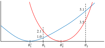
Figure 1: Model parameters are on the x-axis and model losses on the y-axis. Blue and red curves depict losses for clients of cluster $1$ and $2$ respectively. $\theta^{*}_{1}$ and $\theta^{*}_{2}$ are optimal models for clients of clusters $1$ and $2$ respectively. Initial models are $\theta_{1}$ and $\theta_{2}$. Loss on model $\theta_{1}$ ($\theta_{2}$) is $1.0$ ($5.1$) and $2.1$ ($3.5$) for clients of clusters $1$ and $2$, respectively. Loss vectors are $[1.0,5.1]$ for clients of cluster $1$ and $[2.1,3.5]$ for clients of cluster $2$. In IFCA, all clients select model $\theta_{1}$, as it minimizes their loss. Consequently they all get assigned to cluster $1$. Moreover, because of this assignment, model $\theta_{2}$ receives no updates, and therefore its loss stays high; as a result, no clients ever select it in future rounds. Ultimately, this leads to all clients converging to the same cluster, failing to recover the true client clusters. In contrast, clustering based on loss vectors achieves accurate client partitioning, as the loss vectors of clients from different clusters are highly distinct.

An alternative way to recover cluster assignments is to leverage the separation of cluster-specific models. For instance, the Iterative Federated Clustering Algorithm (IFCA) IFCA_paper_2020 assigns clients to clusters based on the model that yields the lowest empirical loss. However, IFCA has a significant limitation: it requires careful initialization of cluster models, ensuring each model is sufficiently close to its optimal counterpart. Specifically, the distance between an initial model and the cluster’s optimal model must be strictly less than half the minimum separation distance between any two optimal models. In practice, achieving this distance requirement can be challenging. For example, in our experiments with the MNIST dataset, IFCA often failed to recover accurate cluster assignments. As shown in Fig. 1, this issue typically occurs when clients from two or more clusters achieve the lowest loss on the same model, and thus get assigned to the same cluster. This, in turn, causes the algorithm to get stuck and fail to recover accurate clusters.

In this paper, we propose the Clustering of Loss Vector Embeddings (CLoVE) PFL algorithm, a novel approach to tackle both the challenges of constructing accurate cluster-specific models and recovering the underlying cluster assignments in a FL setting. Our solution employs an iterative process that simultaneously builds multiple personalized models and generates client embeddings, represented as vectors of losses achieved by these models on the clients’ local data. Specifically, we leverage the clustering of client embeddings to refine the models, while also using the models to inform the clustering process. The underlying principle of our approach is that clients within the same cluster will exhibit similar loss patterns, whereas those from different clusters will display distinct loss patterns across models. By analyzing and comparing these loss patterns through the clustering of loss vectors, our approach effectively separates clients from different clusters while grouping those from the same cluster together. This, in turn, leads to improved models for each cluster, as each model predominantly receives updates from clients within its corresponding cluster, thereby enhancing accuracy and robustness.

Similar to IFCA, our approach also exploits the separation of cluster-specific models and does not rely on assumptions about the data distributions of clusters. However, unlike IFCA, which for accurate cluster recovery requires that clients from the same cluster achieve the lowest loss on the same unique model, our method relies solely on the loss vectors of clients from different clusters being well-separated. As depicted in Figure 1, the separation of loss vectors among clients from different clusters is highly likely, regardless of the model initialization, since such clients’ local data is likely to incur different losses on any given model. Notably, we demonstrate (proof in Appendix, Lemma A.17) that the cluster recovery condition of IFCA implies loss vector separation among clients of different clusters, but as illustrated in Figure 1, the converse is not always true.

We conduct a comprehensive evaluation of our approach, demonstrating its ability to recover clusters with high accuracy while constructing per-cluster models in just a few rounds of FL. Furthermore, our analytical results show that our approach can achieve single-shot, accurate cluster recovery with high probability in the case of linear regression, thereby establishing its efficacy and robustness.

Our technical contributions can be summarized as follows:

• Introduction of the CLoVE PFL algorithm: We propose a novel approach that simultaneously builds multiple personalized models and generates client embeddings based on model losses, enabling effective clustering of clients with unknown cluster labels.

• Simplicity and wide applicability: Our method, unlike most others, extends to both supervised and unsupervised settings, handling a variety heterogeneous data distributions through a simple, loss-based embedding approach.

• Robustness against initialization: Unlike existing methods, CLoVE does not require careful initialization of cluster models, thereby mitigating the risk of inaccurate cluster assignments due to initialization sensitivities.

• Theoretical guarantees for cluster recovery: We provide analytical results showing that, in the context of linear regression, CLoVE can achieve single-shot, accurate cluster recovery with high probability.

• Efficient cluster recovery and model construction: We demonstrate through comprehensive evaluations that CLoVE can recover the true clusters with high accuracy and construct per-cluster models within a few rounds of federated learning in a variety of settings.

2 Related Work

A primary challenge in FL is handling heterogeneous data distributions (non-IID data) and varying device capabilities. Early optimization methods like FedAvg mcmahan2017communication and FedProx li2019convergence mitigate some issues by allowing multiple local computations before aggregation, yet they typically yield a single global model that may not capture the diversity across user populations zhao2018federated .

Personalized Federated Learning (PFL) hanzely2020federated ; tan2023towards aims to deliver client-specific models that outperform both global models and naïve local baselines. Various strategies have been proposed, including fine-tuning global models locally fallah_personalized_2020_Per-FedAvg or performing adaptive local aggregation zhang_FedALA_2023 , meta-learning jiang2023improving , multi-task learning smith2017federated ; xu_personalized_2023_FedPAC , and decomposing models into global and personalized components deng2020adaptive ; mansour2020three . However, these methods operate in a supervised setting and require labeled data.

Clustered Federated Learning (CFL) is an emerging approach in PFL that involves clustering clients based on similarity measures to train specialized models for each cluster (e.g. IFCA IFCA_paper_2020 based on model loss values, Werner_2023 ; kim2024 and FlexCFL duan_flexible_2022_FlexCFL based on gradients). Sattler_2021_CFL ’s CFL algorithm utilizes federated multitask learning and gradient embeddings in order to iteratively form and refine clusters. vahidian_efficient_2023_PACFL ’s PACFL algorithm derives a set of principal vectors from each cluster’s data, and FedProto tan_fedproto_2022 constructs class prototypes, which allow the server to identify distribution similarities.

Traditional clustering methods, such as spectral clustering and k-means, have also been adapted for federated scenarios. In long_multicenter_2023_FeSEM , personalization is achieved by deriving the optimal matching of users and multiple model centers, and in chen_spectral_2023 through spectral co-distillation. Despite their effectiveness, these methods often require complex similarity computations or additional communication steps.

Recent advancements in CFL have focused on enhancing convergence and reducing reliance on initial cluster assignments. Improved algorithms improved_clustered_fed2024 address some limitations of earlier approaches that require careful initialization like IFCA_paper_2020 , but their methods are complex. Our CLoVE algorithm overcomes these drawbacks using a simple method that utilizes robust loss-based embeddings, converges quickly to the correct clusters, eliminates the need for precise initialization, and operates in a variety of both supervised and unsupervised settings.

3 Embeddings-driven Federated Clustering

The typical FL architecture consists of a server and a number of clients. Let $M$ be the number of clients, which belong to $K$ clusters. Clients in each of the $K$ clusters draw data from a distinct data distribution $D_{j}$, $j\in[K]$ (where the notation $[K]$ denotes the set $\{1,2,...,K\}$). Each client $i\in[M]$ has $n_{i}$ data points. Let $f(\theta;z):\Theta\rightarrow\mathbb{R}$ be the loss function associated with data point $z$, where $\Theta\subseteq\mathbb{R}^{d}$ is the parameter space. The goal in FL is to minimize the population loss function $\mathcal{L}_{j}(\theta)\triangleq\mathbb{E}_{z\sim D_{j}}[f(\theta;z)]$ for all $j\in[K]$. Let the empirical loss for the data $Z_{i}$ of client $i$ be defined as $\mathcal{L}^{i}(\theta;Z_{i})\triangleq(1/|Z_{i}|)\sum_{z\in Z_{i}}f(\theta;z)$. The goal of a PFL algorithm is to simultaneously cluster the clients into $K$ clusters and train $K$ models, each of which each of which is best suited for the data of a single client cluster.

1

2

Input: # of clients $M$, # of true clusters (and # of models) $K$, # of data points $n_{i}$ for client $i$, $i\in[M]$

Hyperparameters : learning rate $\gamma$, # of rounds $T$, # of local epochs $\tau$ (for model averaging)

Output: final model parameters $\theta_{j}^{(T)},j\in[K]$

3

4Server: initialize model parameters $\theta_{j}^{(0)}$ for each of the $K$ models $j\in[K]$

5for round $t=0,1,...,T-1$ do

6    $M^{(t)}\leftarrow$ random subset of clients

7   

8   Server: broadcast model parameters $\theta_{j}^{(t)}$ of all $K$ models $j\in[K]$ to all clients in $M^{(t)}$

9   

10   for each client $i\in M^{(t)}$ in parallel do

11       Run client $i$’s data through all $K$ models and get the losses $\mathcal{L}^{i,{(t)}}\triangleq\left(\mathcal{L}^{i}(\theta_{j}^{(t)})\right),j\in[K]$

12      Send loss vector $\mathcal{L}^{i,{(t)}}$ to the server

13   

14   Server (clustering step):

15    – Run vector clustering algorithm to group the set of vectors $\{\mathcal{L}^{i,{(t)}},i\in[M]\}$ into $K$ client clusters

16   

17   – Map client clusters to models using min-cost matching and assign each client $i\in M^{(t)}$ to the corresponding model $c_{i}\equiv c_{i}^{(t)}\in[K]$ of its client cluster

18   for each client $i\in M^{(t)}$ in parallel do

19       – Option I (model averaging): Compute new model parameters $\widetilde{\theta}_{i}=\text{LocalUpdate}(i,\theta_{c_{i}}^{(t)},\gamma,\tau)$ for model $c_{i}$ and send them to the server

20      – Option II (gradient averaging): Compute stochastic gradient $g_{i}=\widehat{\nabla}\mathcal{L}^{i}(\theta_{c_{i}}^{(t)})$ using $c_{i}$’s model and send it to the server

21   

22   Server (averaging step):

23    Clients that were assigned to model $j$ at round $t$: $C_{j}^{(t)}\triangleq\{i\in M^{(t)}\text{ s.t. }c_{i}^{(t)}=j\}$

24   

25   – Option I (model averaging): $\forall~j\in[K]\text{ s.t. }C_{j}^{(t)}\neq\emptyset$, $\theta_{j}^{(t+1)}=\dfrac{\sum_{i\in C_{j}^{(t)}}n_{i}\widetilde{\theta}_{i}}{\sum_{i\in C_{j}^{(t)}}n_{i}}$

26   – Option II (gradient averaging): $\forall~j\in[K]\text{ s.t. }C_{j}^{(t)}\neq\emptyset$, $\theta_{j}^{(t+1)}=\theta_{j}^{(t)}-\gamma\dfrac{\sum_{i\in C_{j}^{(t)}}n_{i}g_{i}}{\sum_{i\in C_{j}^{(t)}}n_{i}}$

27   

28

29return $\theta_{j}^{(T)}$

Algorithm 1 Clustering of Loss Vector Embeddings (CLoVE) algorithm for PFL

The pseudocode of our Clustering of Loss Vector Embeddings (CLoVE) PFL algorithm is shown in Alg. 1. The algorithm operates as follows. Initially, the server creates $K$ models (line 1), each of which will eventually get trained to fit the data of each of the $K$ clusters, and sends all of them to a subset (or all) of the $M$ clients (lines 3-4). Each of these clients runs its data through all $K$ models and gets the losses, which form one loss vector of length $K$ per client. These loss vectors are then sent to the server (lines 5-7). The server treats the loss vectors as data points and runs a vector clustering algorithm (e.g. k-means) on them in order to cluster them into $K$ groups (line 9) using a minimum-cost matching algorithm: a bipartite graph is created, with the nodes being the client clusters on the left and the models on the right, and the weight of each edge being the sum of the losses of the clients in the cluster on the left on the model on the right (another weight option can be the cluster’s overlap with the previous clusters). We find the minimum cost bipartite matching using standard methods (e.g. max-flow-based). Subsequently, each client (represented by its corresponding loss vector) is assigned to a certain cluster $c_{i}$ (and effectively to the cluster’s corresponding model) for that iteration (line 10). Then, each client trains its assigned model on its private data (lines 11-12) by running locally $\tau$ steps of a gradient descent optimization algorithm denoted by the function $\text{LocalUpdate}(\cdot)$ (e.g. Stochastic Gradient Descent (SGD), Adaptive Moment Estimation (Adam) Adam_paper , etc.) starting with model $c_{i}$’s parameters, and sends the resulting model parameters to the server. Then, the averaging step follows: the server aggregates all the received model parameters for each model $j$ from the set $C_{j}^{(t)}$ of clients that updated it, using a weighted average, where each client $i$’s contribution is normalized by its number of samples $n_{i}$ (lines 13-15). In the next iteration, the server sends the computed updated parameters once again to the clients (line 4), and the process continues.

Another variant of CLoVE emerges if we replace model averaging with gradient averaging. The difference is that the order of taking a gradient step and of averaging has been reversed. Now, each client computes the gradient of the loss function with respect to its assigned model by the server ($c_{i}$) (line 12) and sends the gradient to the server. Then the server takes a weighted average of the gradients, where each client $i$’s gradient is normalized by its number of samples $n_{i}$, and subtracts the aggregated gradient multiplied by the learning rate from the previous parameters, to get the new parameters (line 15).

Note that our algorithm is a generalization of FedAvg, the original FL algorithm mcmahan2017communication , in which a single model is being trained by all clients. If we set $K=1$ in CLoVE, then lines 5-10 become trivial, all clients train the same model in lines 11-12 and the server aggregates the updated parameters from all clients together in lines 13-15. Note also that despite the fact that privacy is an important concern in FL, it is not the focus of this paper. The fact that clients send their loss vectors to the server for clustering does not reveal anything about their data, nor any information beyond (indirectly) the cluster each client belongs to, which anyway is information that the server needs to aggregate the models in any PFL setting.

4 Theoretical analysis of CLoVE’s performance

We now provide theoretical evidence supporting the superior performance of CLoVE. In the following we omit all proofs, which can be found in Appendix A. To analyze the efficacy of CLoVE, we consider a mixed linear regression problem yi2014alternating in a federated learning setting IFCA_paper_journal_version_2022 . In this context, each client’s data originates from one of $K$ distinct clusters, denoted as $\mathcal{C}_{1},\mathcal{C}_{2},\dots,\mathcal{C}_{K}$. Within each cluster $\mathcal{C}_{k}$, the data pairs $z_{i}=(x_{i},y_{i})$ are drawn from the same underlying distribution $\mathcal{D}_{k}$, which is generated by the linear model:

$$y_{i}=\langle\theta^{*}_{k},x_{i}\rangle+\epsilon_{i}.$$

Here, the feature $x_{i}$ follows a standard normal distribution $\mathcal{N}(0,I_{d})$, and the additive noise $\epsilon_{i}$ follows a normal distribution $\mathcal{N}(0,\sigma^{2})$ ($\sigma\ll 1$), both independently drawn. The loss function is the squared error: $f(\theta;x,y)=\left(\langle\theta,x\rangle-y\right)^{2}.$ Under this setting, the parameters $\theta^{*}_{k}\in\mathbb{R}^{d}$ are the minimizers of the population loss for cluster $\mathcal{C}_{k}$.

At a high level, our analysis unfolds as follows. We demonstrate that by setting the entries of a client’s loss vector (SLV) to the square root of model losses, CLoVE can accurately recover client clustering with high probability in each round. This, in turn, enables CLoVE to accurately match clients to models with high probability by utilizing the minimum-cost bipartite matching between clusters and models. Consequently, we show that the distance between the models constructed by CLoVE and their optimal counterparts decreases exponentially with the number of rounds, following the application of client gradient updates, thus implying fast convergence of CLoVE to optimal models.

For our analysis we make some assumptions, including that all $\theta^{*}_{i}\in\mathbb{R}^{d}$ have unit norms and their minimum separation $\Delta>0$ is close to $1$. We also assume the number of clusters $K$ is small in comparison to the total number of clients $M$ and the dimension $d$. We assume that each client of cluster $k$ uses the same number $n_{k}$ of i.i.d. data points independently chosen at each round.

For a given model $\theta$, the empirical loss $\mathcal{L}_{k}^{i}(\theta)$ for a client $i$ in cluster $k$ is:

$$\frac{1}{n_{k}}\sum_{j=1}^{n_{k}}\left(\langle\theta,x_{j}\rangle-y_{j}\right)^{2}=\frac{1}{n_{k}}\sum_{j=1}^{n_{k}}\left(\langle\theta^{*}_{k}-\theta,x_{j}\rangle+\epsilon_{j}\right)^{2}$$

For a given collection of $N$ models, $\boldsymbol{\theta}=\begin{bmatrix}\theta_{1}&\theta_{2}&\cdots&\theta_{N}\end{bmatrix}$, and the square root loss vector (SLV) of a client $i$ of cluster $k$ is $a_{k}^{i}(\boldsymbol{\theta})=[F_{k}^{i}(\theta_{1}),F_{k}^{i}(\theta_{2}),\ldots F_{k}^{i}(\theta_{N})]$. Here $F_{k}^{i}(\theta)=\sqrt{\mathcal{L}_{k}^{i}(\theta)}\sim\frac{\alpha(\theta,\theta_{k}^{*})}{\sqrt{n_{k}}}\chi(n_{k})$, where $\alpha(\theta,\theta_{k}^{*})=\sqrt{\|\theta-\theta_{k}^{*}\|^{2}+\sigma^{2}}$, and $\chi(n_{k})$ denotes a standard chi random variable with $n_{k}$ degrees of freedom. Let $c_{k}(\boldsymbol{\theta})=\left[\mathbb{E}[F_{k}^{i}(\theta_{1})],\mathbb{E}[F_{k}^{i}(\theta_{2})],\ldots,\mathbb{E}[F_{k}^{i}(\theta_{N})]\right]$ denote the distribution mean of the SLVs for a cluster $k$. We say a model collection $\boldsymbol{\theta}$ is $\Delta$-proximal if each $\theta_{k}$ is within a distance at most $\Delta/4$ of its optimal counterpart $\theta_{k}^{*}$. For our analysis we assume CLoVE is initialized with a set $\boldsymbol{\theta}$ of ortho-normal models. In the following $m_{k}$ denotes the number of clients in cluster $k$ and $n=\min_{k}n_{k}$.

One of our key results is the following.

Theorem 4.1.

For both ortho-normal or $\Delta$-proximal models collections, k-means clustering of SLVs, with suitably initialized centers, recovers accurate clustering of the clients in one shot. This result holds with probability at least $\xi=1-\delta-\frac{1}{\mbox{polylog}(M)}$, for any error tolerance $\delta$.

We prove this by showing that, for such model collections, the mixture of distributions formed by the collection of SLVs from different clients satisfies the proximity condition of kumar2010clustering . Specifically, it is shown in Theorem A.9 that when the number of data points across all clients is much larger than $d,K$, then for any client $i$, with probability at least $\xi$:

$$\forall~{j^{\prime}\neq j},~\|a_{j}^{i}(\boldsymbol{\theta})-c_{j^{\prime}}(\boldsymbol{\theta})\|-\|a_{j}^{i}(\boldsymbol{\theta})-c_{j}(\boldsymbol{\theta})\|\geq\left(\frac{c^{\prime}K}{m_{i}}+\frac{c^{\prime}K}{m_{j}}\right)\|A(\boldsymbol{\theta})-C(\boldsymbol{\theta})\|$$

Here $c^{\prime}$ is a large constant and client $i$ is assumed to belong to cluster $j$. Theorem 4.1 then follows directly from the result of kumar2010clustering .

The proof of Theorem A.9 is based on a sequence of intermediate results. In particular, Lemma A.1 and Lemma A.2 demonstrate that, for the ortho-normal and $\Delta$-proximal model collections, the means of the SLV distributions across distinct clusters are sufficiently well-separated:

For any $i\neq j$, $\|c_{i}(\boldsymbol{\theta})-c_{j}(\boldsymbol{\theta})\|\geq\dfrac{\Delta}{c}$. Here, $c\approx 2$.

Furthermore, Lemma A.4 shows that with high probability, SLVs of each cluster are concentrated around their means. We use these results, combined with a result of dasgupta2007spectral to prove Lemma A.7 which establishes that the norm of the matrix $X(\boldsymbol{\theta})$ of “centered SLVs”, whose $i$-th row is $a_{s(i)}^{i}(\boldsymbol{\theta})-c_{s(i)}(\boldsymbol{\theta})$, is bounded. That is, for $\gamma=\sqrt{d\frac{1}{2n}\left(9+\sigma^{2}\right)}$, with high probability: $\|X(\boldsymbol{\theta})\|\leq\gamma\sqrt{M}\mbox{polylog}(M)$. By combining these results, we are able to derive the proximity condition of Theorem A.9.

Next, we prove our second key result, that models constructed by CLoVE converge exponentially fast towards their optimal counterpart. Let $\boldsymbol{\theta}^{i}$ denote model collection at round $i$.

Theorem 4.2.

After $T$ rounds, each model $\theta_{k}\in\boldsymbol{\theta}^{T}$ satisfies $\|\theta_{k}-\theta^{*}_{k}\|\leq\dfrac{\Delta}{c_{1}^{T}}$, with high probability, for a constant $c_{1}$.

In the first round, the models $\boldsymbol{\theta}^{1}$ for CLoVE are initialized to be ortho-normal, ensuring accurate cluster recovery by Theorem 4.1. Under the assumption that for all clusters $k$, $n_{k}m_{k}\left(\frac{\rho}{\rho+1}\right)^{2}\gg\mbox{polylog}(K)$, where $\rho=\Delta^{2}/\sigma^{2}$, Lemma A.16 shows that the min-cost bi-bipartite matching found by CLoVE yields an optimal client-to-model match with probability close to 1. Furthermore, Lemma A.13 demonstrates that as a consequence of this optimal match, the updated models $\boldsymbol{\theta}^{2}$, obtained by applying gradient updates from clients to their assigned models, are $\Delta$-proximal with high probability, provided that the learning rate $\eta$ is suitably chosen.

In subsequent rounds, the $\Delta$-proximality of the models $\boldsymbol{\theta}^{2}$ enables the application of a similar argument, augmented by Corollary A.14. With high probability, this implies that the updated models $\boldsymbol{\theta}^{3}$ not only remain $\Delta$-proximal, but also have a distance to their optimal counterparts that is a constant fraction $c_{1}$ times smaller, resulting from the gradient updates from their assigned clients. Thus, by induction, the proof of Theorem 4.2 follows, provided $\delta T\ll 1$.

5 Performance Evaluation

We now show how our algorithms perform compare to the state of the art in both supervised and unsupervised settings.

5.1 Experimental Setup

Datasets and Models

We evaluate our method on three types of tasks – image classification, text classification, and image reconstruction – using five widely-used datasets: MNIST: handwritten digit images (10 classes), Fashion-MNIST (FMNIST): clothing items (10 classes), CIFAR-10: colored natural images (10 classes), Amazon Reviews: text-based sentiment classification (binary – positive/negative), and AG News: news article classification (4 categories). For the classification tasks, we use three different convolutional neural networks (CNNs): a shared CNN model for MNIST and FMNIST, a deeper CNN for CIFAR-10, a TextCNN for AG News, and an MLP-based model (AmazonMLP) for Amazon Reviews. For the unsupervised image reconstruction tasks on MNIST and FMNIST, we use a simple autoencoder, while a convolutional autoencoder is employed for CIFAR-10. Further details about these datasets and model architectures can be found in App. B.

Table 1: Supervised test accuracy results for MNIST, CIFAR-10 and FMNIST

Algorithm	Data mixing	MNIST	CIFAR-10	FMNIST	Data mixing	MNIST	CIFAR-10	FMNIST
FedAvg	Label skew 1	$87.4\pm 0.9$	$34.0\pm 3.6$	$64.7\pm 1.2$	Concept shift	$52.4\pm 0.3$	$\mathbf{63.1\pm 1.7}$	$49.1\pm 0.1$
Local-only		$99.5\pm 0.1$	$85.4\pm 1.6$	$98.8\pm 0.1$		$94.8\pm 0.3$	$45.1\pm 0.4$	$78.3\pm 0.4$
Per-FedAvg		$97.8\pm 0.2$	$75.0\pm 0.7$	$97.0\pm 0.1$		$80.2\pm 1.0$	$34.9\pm 0.7$	$70.4\pm 1.0$
FedProto		$99.2\pm 0.0$	$83.0\pm 0.3$	$98.6\pm 0.0$		$95.0\pm 0.4$	$40.8\pm 0.3$	$78.4\pm 0.3$
FedALA		$98.9\pm 0.1$	$80.0\pm 0.6$	$97.8\pm 0.0$		$96.7\pm 0.2$	$42.0\pm 1.0$	$81.1\pm 0.3$
FedPAC		$94.4\pm 0.7$	$78.3\pm 0.4$	$91.7\pm 1.2$		$90.7\pm 1.3$	$39.0\pm 1.0$	$73.8\pm 0.6$
CFL		$82.5\pm 21.8$	$87.4\pm 0.4$	$65.8\pm 22.4$		$97.5\pm 0.2$	$35.7\pm 3.2$	$83.7\pm 0.5$
FeSEM		$73.2\pm 0.8$	$11.2\pm 1.6$	$41.8\pm 0.7$		$46.2\pm 0.1$	$12.7\pm 0.5$	$39.7\pm 0.6$
FlexCFL		$99.4\pm 0.0$	$73.2\pm 0.3$	$99.0\pm 0.1$		$97.4\pm 0.1$	$17.8\pm 2.1$	$\mathbf{86.1\pm 0.2}$
PACFL		$99.1\pm 0.1$	$79.1\pm 1.0$	$98.7\pm 0.1$		$93.3\pm 0.1$	$26.8\pm 1.2$	$72.6\pm 1.2$
IFCA		$99.1\pm 0.5$	$85.7\pm 6.5$	$97.8\pm 1.9$		$80.0\pm 0.2$	$52.7\pm 4.7$	$67.0\pm 6.2$
CLoVE		$\mathbf{99.8\pm 0.0}$	$\mathbf{90.5\pm 0.1}$	$\mathbf{99.1\pm 0.0}$		$\mathbf{97.6\pm 0.1}$	$58.4\pm 0.6$	$84.3\pm 0.2$
FedAvg	Label skew 2	$76.4\pm 0.3$	$47.7\pm 4.0$	$55.2\pm 1.6$	Feature skew	$90.0\pm 0.6$	$52.4\pm 2.5$	$76.5\pm 0.3$
Local-only		$94.2\pm 0.2$	$55.9\pm 1.8$	$86.1\pm 0.4$		$93.0\pm 0.1$	$38.5\pm 1.6$	$75.8\pm 0.2$
Per-FedAvg		$94.9\pm 0.6$	$48.2\pm 0.9$	$78.2\pm 1.0$		$87.8\pm 0.5$	$22.8\pm 0.1$	$66.7\pm 0.4$
FedProto		$94.4\pm 0.2$	$56.8\pm 0.8$	$82.1\pm 0.9$		$92.3\pm 0.3$	$34.1\pm 0.2$	$74.0\pm 0.3$
FedALA		$95.1\pm 0.3$	$50.1\pm 1.6$	$81.6\pm 0.7$		$90.2\pm 0.6$	$22.3\pm 0.4$	$68.1\pm 0.5$
FedPAC		$91.9\pm 0.5$	$40.7\pm 5.2$	$77.6\pm 1.2$		$87.6\pm 0.4$	$24.6\pm 0.2$	$67.4\pm 0.2$
CFL		$\mathbf{97.3\pm 0.3}$	$62.1\pm 0.4$	$87.2\pm 1.2$		$95.1\pm 0.2$	$\mathbf{61.6\pm 5.1}$	$77.8\pm 3.5$
FeSEM		$89.1\pm 1.6$	$15.3\pm 2.5$	$51.4\pm 0.2$		$79.5\pm 0.4$	$10.7\pm 0.5$	$67.6\pm 0.5$
FlexCFL		$95.6\pm 0.3$	$43.6\pm 0.6$	$88.7\pm 0.2$		$96.7\pm 0.1$	$12.2\pm 0.4$	$\mathbf{85.2\pm 0.2}$
PACFL		$92.0\pm 1.1$	$40.4\pm 1.0$	$81.1\pm 0.5$		$89.3\pm 0.1$	$17.1\pm 0.6$	$70.6\pm 0.6$
IFCA		$96.8\pm 0.2$	$63.4\pm 3.4$	$89.4\pm 1.3$		$95.9\pm 2.0$	$50.8\pm 7.0$	$83.5\pm 0.3$
CLoVE		$97.1\pm 0.3$	$\mathbf{66.8\pm 2.3}$	$\mathbf{90.1\pm 0.3}$		$\mathbf{97.7\pm 0.1}$	$57.1\pm 1.8$	$85.1\pm 0.2$

Dataset Partitioning

Similar to vahidian_efficient_2023_PACFL ; duan_flexible_2022_FlexCFL ; xu_personalized_2023_FedPAC ; zhang_FedALA_2023 ; IFCA_paper_2020 , we simulate data heterogeneity by randomly partitioning data across clusters of clients, without replacement, with various types of skews, including label and feature skews, as well as concept shifts. For label skew, we consider both non-overlapping and overlapping label distributions. In case Label skew 1, clients within each cluster receive data from only two unique classes, with no label overlap between clients in different clusters. Conversely, in case Label skew 2, each client within each cluster receives samples from $U$ classes, with at least $V$ labels shared between the labels assigned to any two clusters. For the AG News dataset, we use $U=2$ and $V=1$, while for all image datasets we use $U=4$ and $V=2$. To simulate feature distribution shifts, we apply image rotations (0°, 90°, 180°, 270°) to the MNIST dataset. Each client within a cluster is assigned data with a specific rotation. Concept shift is achieved through label permutation: all labels are distributed across all clusters, but clients within each cluster receive data with two unique label swaps. Both test and train data of a client have the same distribution.

Compared Methods

We compare the following baselines: Local-only, where each client trains its model locally; FedAvg mcmahan2017communication , which learns a single global model; clustered federated learning methods, including CFL Sattler_2021_CFL , IFCA IFCA_paper_2020 , FlexCFL duan_flexible_2022_FlexCFL , FeSEM long_multicenter_2023_FeSEM , and PACFL vahidian_efficient_2023_PACFL ; and general PFL methods FedProto tan_fedproto_2022 , Per-FedAvg fallah_personalized_2020_Per-FedAvg , FedALA zhang_FedALA_2023 , and FedPAC xu_personalized_2023_FedPAC . The source code we used for these algorithms is linked in Table 6.

Training Settings

We use an Adam optimizer, a batch size of 100 and a learning rate $\gamma=10^{-3}$. The number of local training epochs is $\tau=1$ and the number of global communication rounds is $T=100$. For supervised classification tasks we use cross-entropy loss, and for unsupervised tasks we use the MSE reconstruction loss.

Table 2: Supervised ARI results for MNIST, CIFAR-10 and FMNIST

Algorithm	Data mixing	MNIST	CIFAR-10	FMNIST	Data mixing	MNIST	CIFAR-10	FMNIST
CFL	Label skew 1	$0.71\pm 0.20$	$\mathbf{1.00\pm 0.00}$	$0.86\pm 0.20$	Concept shift	$\mathbf{1.00\pm 0.00}$	$0.00\pm 0.00$	$\mathbf{1.00\pm 0.00}$
FeSEM		$0.18\pm 0.00$	$0.00\pm 0.00$	$0.00\pm 0.00$		$0.00\pm 0.00$	$0.00\pm 0.00$	$0.00\pm 0.00$
FlexCFL		$\mathbf{1.00\pm 0.00}$	$\mathbf{1.00\pm 0.00}$	$\mathbf{1.00\pm 0.00}$		$\mathbf{1.00\pm 0.00}$	$0.22\pm 0.24$	$\mathbf{1.00\pm 0.00}$
PACFL		$0.39\pm 0.07$	$0.60\pm 0.09$	$\mathbf{1.00\pm 0.00}$		$-0.00\pm 0.02$	$0.00\pm 0.00$	$0.00\pm 0.00$
IFCA		$0.83\pm 0.12$	$0.91\pm 0.13$	$0.92\pm 0.12$		$0.68\pm 0.00$	$0.76\pm 0.17$	$0.55\pm 0.18$
CLoVE		$\mathbf{1.00\pm 0.00}$	$\mathbf{1.00\pm 0.00}$	$\mathbf{1.00\pm 0.00}$		$\mathbf{1.00\pm 0.00}$	$\mathbf{1.00\pm 0.00}$	$\mathbf{1.00\pm 0.00}$
CFL	Label skew 2	$0.00\pm 0.00$	$0.72\pm 0.00$	$0.57\pm 0.00$	Feature skew	$0.48\pm 0.00$	$0.89\pm 0.15$	$0.16\pm 0.23$
FeSEM		$0.18\pm 0.00$	$0.00\pm 0.00$	$0.00\pm 0.00$		$0.00\pm 0.00$	$0.00\pm 0.00$	$0.00\pm 0.00$
FlexCFL		$\mathbf{1.00\pm 0.00}$	$\mathbf{1.00\pm 0.00}$	$\mathbf{1.00\pm 0.00}$		$\mathbf{1.00\pm 0.00}$	$0.11\pm 0.08$	$\mathbf{1.00\pm 0.00}$
PACFL		$0.35\pm 0.12$	$0.32\pm 0.11$	$0.55\pm 0.03$		$0.00\pm 0.00$	$0.00\pm 0.00$	$0.68\pm 0.11$
IFCA		$0.83\pm 0.12$	$0.81\pm 0.13$	$0.92\pm 0.12$		$0.67\pm 0.28$	$0.71\pm 0.22$	$0.55\pm 0.10$
CLoVE		$\mathbf{1.00\pm 0.00}$	$\mathbf{1.00\pm 0.00}$	$\mathbf{1.00\pm 0.00}$		$\mathbf{1.00\pm 0.00}$	$\mathbf{1.00\pm 0.00}$	$\mathbf{1.00\pm 0.00}$

Result reporting

We report the average performance of the models assigned to the clients on their local test data. Specifically, we report test accuracies for supervised classification tasks and reconstruction losses for unsupervised tasks. In addition, we report the accuracy of client-to-cluster assignments as the Adjusted Rand Index (ARI) between the achieved clustering and the ground-truth client groupings. To account for randomness, we run each experiment for 3 values of a randomness seed and report the mean and standard deviation.

5.2 Numerical results

Table 3: Supervised test accuracy results for Amazon Review and AG News

Algorithm	Amazon	AG News
FedAvg	$\mathbf{99.0\pm 0.1}$	$40.2\pm 0.1$
Local-only	$81.2\pm 0.4$	$51.4\pm 1.1$
Per-FedAvg	$87.7\pm 0.4$	$48.0\pm 1.1$
FedProto	$81.3\pm 0.1$	$18.9\pm 1.5$
FedALA	$88.3\pm 0.3$	$49.6\pm 0.1$
FedPAC	$88.2\pm 0.2$	$42.4\pm 2.9$
CFL	$87.7\pm 0.8$	$48.4\pm 2.7$
FeSEM	$50.9\pm 0.2$	$19.1\pm 1.5$
FlexCFL	$84.1\pm 0.8$	$\mathbf{60.2\pm 5.5}$
PACFL	$82.1\pm 0.3$	$51.1\pm 1.9$
IFCA	$85.5\pm 0.5$	$51.3\pm 3.3$
CLoVE	$86.8\pm 0.4$	$55.1\pm 0.2$

Our experiments involve varying the number of clients between 20 and 100, and distributing them across clusters ranging from 4 to 10. In most cases, the training data size per client is set to 500. However, for the Amazon Reviews and AG News datasets, we use 1000 and 100 samples, respectively. The test accuracies for image classification tasks are reported in Table 1. The results demonstrate that CLoVE performs consistently well across various data distributions, including label and feature skews, as well as concept shifts. While some baseline algorithms exhibit strong performance in specific cases, CLoVE is the only algorithm that consistently ranks among the top performers in almost all scenarios.

Table 4: Convergence behavior for MNIST, CIFAR-10 and FMNIST

Data mixing	Algorithm	% of final ARI reached in 10 rounds			First round when ARI $\geq 90\%$
		MNIST	CIFAR-10	FMNIST	MNIST	CIFAR-10	FMNIST
Label skew 1	CFL	$0.0\pm 0.0$	$0.0\pm 0.0$	$0.0\pm 0.0$	$25.3\pm 2.1$	$41.3\pm 2.1$	$28.3\pm 2.9$
	FeSEM	$\mathbf{100.0\pm 0.0}$	$0.0\pm 0.0$	$0.0\pm 0.0$	$\mathbf{1.0\pm 0.0}$	—	—
	FlexCFL	$\mathbf{100.0\pm 0.0}$	$\mathbf{100.0\pm 0.0}$	$\mathbf{100.0\pm 0.0}$	$\mathbf{1.0\pm 0.0}$	$\mathbf{1.0\pm 0.0}$	$\mathbf{1.0\pm 0.0}$
	PACFL	$\mathbf{100.0\pm 0.0}$	$\mathbf{100.0\pm 0.0}$	$\mathbf{100.0\pm 0.0}$	$\mathbf{1.0\pm 0.0}$	$\mathbf{1.0\pm 0.0}$	$\mathbf{1.0\pm 0.0}$
	IFCA	$\mathbf{100.0\pm 0.0}$	$81.3\pm 13.2$	$91.7\pm 11.8$	$2.0\pm 0.0$	$11.3\pm 6.6$	$7.3\pm 7.5$
	CLoVE	$\mathbf{100.0\pm 0.0}$	$\mathbf{100.0\pm 0.0}$	$\mathbf{100.0\pm 0.0}$	$2.0\pm 0.0$	$2.0\pm 0.0$	$2.0\pm 0.0$
Concept shift	CFL	$0.0\pm 0.0$	$0.0\pm 0.0$	$0.0\pm 0.0$	$60.0\pm 9.4$	—	$43.0\pm 5.7$
	FeSEM	$0.0\pm 0.0$	$0.0\pm 0.0$	$0.0\pm 0.0$	—	—	—
	FlexCFL	$\mathbf{100.0\pm 0.0}$	$66.7\pm 47.1$	$\mathbf{100.0\pm 0.0}$	$\mathbf{1.0\pm 0.0}$	$34.0\pm 46.7$	$\mathbf{1.0\pm 0.0}$
	PACFL	$33.3\pm 47.1$	$0.0\pm 0.0$	$0.0\pm 0.0$	$67.0\pm 46.7$	—	—
	IFCA	$\mathbf{100.0\pm 0.0}$	$\mathbf{100.0\pm 0.0}$	$\mathbf{100.0\pm 0.0}$	$2.3\pm 0.5$	$3.0\pm 0.8$	$2.0\pm 0.0$
	CLoVE	$\mathbf{100.0\pm 0.0}$	$\mathbf{100.0\pm 0.0}$	$\mathbf{100.0\pm 0.0}$	$2.0\pm 0.0$	$\mathbf{2.3\pm 0.5}$	$2.0\pm 0.0$

Table 2 presents the clustering accuracies of different CFL algorithms for the image datasets under the same experimental setup. CLoVE achieves optimal performance in all cases. Although FlexCFL also shows near-optimal performance, its accuracy declines when faced with concept shifts, as it neglects label information in similarity estimation. In contrast, loss-based approaches like CLoVE and IFCA excel in this metric, as model losses can effectively account for various types of skews. Results for additional types of label skews (e.g. dominant class xu_personalized_2023_FedPAC ) are included in App. C.1.2.

The test accuracies for the textual classification tasks are reported in Table 3 (more metrics in App. C.1.3). While CLoVE exhibits good performance here as well, the baseline FedAvg performs especially well on the Amazon Review dataset. One reason is that while the dataset is split by product categories, the underlying language and sentiment cues are still fairly similar across all 4 categories and can provide a good signal for classification. On AG News, CLoVE outperforms all baselines except FlexCFL.

Table 4 presents the clustering recovery speed for the image classification datasets under different client data distributions. The first 3 columns show the percentage of the final ARI that is reached within just 10 rounds (i.e. ARI at round 10 divided by the final ARI, expressed as a percentage) for each algorithm. CLoVE outperforms all baselines here. The next 3 columns show the first round at which an ARI of $90\%$ or higher is achieved (dashes mean 90% ARI is never achieved). As can be seen, CLoVE consistently reaches such high accuracy within 2-3 rounds, unlike any other baseline.

Table 5: Unsupervised test loss results for MNIST, CIFAR-10 and FMNIST

Algorithm	MNIST	CIFAR-10	FMNIST
FedAvg	$0.032\pm 0.001$	$0.026\pm 0.000$	$0.030\pm 0.000$
Local-only	$0.019\pm 0.000$	$0.022\pm 0.000$	$0.170\pm 0.000$
IFCA	$0.024\pm 0.005$	$\mathbf{0.019\pm 0.000}$	$0.020\pm 0.002$
CLoVE	$\mathbf{0.014\pm 0.000}$	$0.021\pm 0.000$	$\mathbf{0.016\pm 0.000}$

Unsupervised Setting

Unlike many of the baselines, CLoVE is equally applicable to unsupervised settings, as it relies solely on model losses to identify clients with similar data distributions. Another loss-based approach, IFCA, serves as a natural point of comparison in this context. As shown in Table 5, CLoVE consistently outperforms IFCA and other baselines in unsupervised settings on image reconstruction tasks using autoencoders, further highlighting its versatility and effectiveness. More experiments in an unsupervised setting can be found in App. C.2.

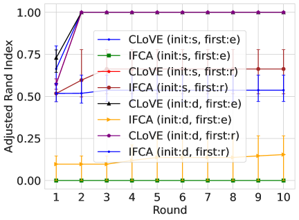
Figure 2: Clustering accuracy of CLoVE and IFCA over time for the initialization experiments

Robustness to initialization

Our results indicate that one key reason CLoVE outperforms related baselines such as IFCA is its robustness to initialization. We evaluate this by varying two factors: the initialization of model parameters and the first round client-to-model assignment strategy. For model initialization, we consider two settings: (1) all models begin with identical parameters (init:s – same), and (2) each model is initialized independently using PyTorch’s default random initialization (init:d – different). For the first round client-to-model assignment, we also explore two approaches: (1) assigning clients to models at random (first:r – random), and (2) assigning clients by clustering their loss vectors (first:e – evaluation-based), followed by bipartite matching as in Alg. 1. Fig. 2 compares CLoVE and IFCA on unsupervised MNIST image reconstruction with 10 clusters, each containing 5 clients with 500 samples. The results show that CLoVE maintains high performance across different initialization methods, unlike IFCA.

5.3 Ablation studies

We analyze the impact of changing some of the key components of CLoVE, one at a time. This includes: (1) No Matching: Order the clusters by their smallest client ID and assign models to them in that order (i.e. cluster $k$ gets assigned model $k$). This is in lieu of using the bi-partite matching approach of Alg. 1. (2) Agglomerative clustering: Use a different method than k-means to cluster the loss vectors. (3) Square root loss: Cluster vectors of square roots of model losses instead of the losses themselves. Our experiments are for image classification for the CIFAR-10 dataset using 25 clients that are partitioned uniformly among 5 clusters using a label skew with very large overlap. The details are provided in App. C.3. We find that “No Matching” has the most impact as it reduces the test accuracy by almost $4.3\%\pm 1\%$. On the other hand, switching to Agglomerative clustering or Square root loss results in no statistically significant gain or loss in performance.

6 Conclusion

We introduced CLoVE, a simple loss vector embeddings-based framework for personalized clustered federated learning that avoids stringent model initialization assumptions and substantially outperforms the state of the art across a range of datasets and in a variety of both supervised and unsupervised settings. In the future, we plan to extend CLoVE to handle online (streaming) data and/or dynamic cluster splits/merges over time. Overall, CLoVE’s design offers a promising and robust approach to scalable model personalization and clustering under heterogeneous data distributions.

Appendix A Linear regression

A.1 Background

We consider a mixed linear regression problem yi2014alternating in a federated setting IFCA_paper_journal_version_2022 . Client’s data come from one of $K$ different clusters, denoted as $\mathcal{C}_{1},\mathcal{C}_{2},\dots,\mathcal{C}_{K}$. Cluster $k$’s optimal model  $\theta^{*}_{k}\in\mathbb{R}^{d}$ is a vector of dimension $d$.

Assumptions: We assume all clients of a cluster $\mathcal{C}_{k}$ use the same number $n_{k}$ of independently drawn feature-response pairs $(x_{i},y_{i})$ in each federated round. These feature-response pairs are drawn from a distribution $\mathcal{D}_{k}$, generated by the model:

$$y_{i}=\langle\theta^{*}_{k},x_{i}\rangle+\epsilon_{i},$$

where $x_{i}\sim\mathcal{N}(0,I_{d})$ are the features, and $\epsilon_{i}\sim\mathcal{N}(0,\sigma^{2})$ represents additive noise. Both are independently drawn. We assume $\sigma$ is very small. Specifically, $\sigma\ll 1$.

We use notation $[K]$ for the set $\{1,2,...,K\}$.

The loss function $f(\theta)$ is defined as the square of the error:

$$f(\theta;x,y)=\left(\langle\theta,x\rangle-y\right)^{2}.$$

The population loss for cluster $k$ is:

$$\mathcal{L}_{k}(\theta)=\mathbb{E}_{(x,y)\sim\mathcal{D}_{k}}\left[\left(\langle\theta,x\rangle-y\right)^{2}\right],$$

Note that the optimal parameters $\{\theta^{*}_{k}\}_{k=1}^{K}$ are the minimizers of the population losses $\{\mathcal{L}_{k}\}_{k=1}^{K}$, i.e.,

$$\theta^{*}_{k}=\arg\min_{\theta}\mathcal{L}_{k}(\theta)\quad\text{for each }k\in[K].$$

We assume these optimal models have unit norm. That is $\|\theta^{*}_{k}\|=1$ for all $k$. We also assume the optimal models are well-separated. That is, there exists a $\Delta>0$ such that for any pair $i\neq j$:

$$\|\theta^{*}_{i}-\theta^{*}_{j}\|\geq\Delta$$

For a given $\theta$, the empirical loss for client $i$ in cluster $k$ is:

$$\mathcal{L}_{k}^{i}(\theta)=\frac{1}{n_{k}}\sum_{j=1}^{n_{k}}\left(\langle\theta,x_{j}\rangle-y_{j}\right)^{2}=\frac{1}{n_{k}}\sum_{j=1}^{n_{k}}\left(\langle\theta^{*}_{k}-\theta,x_{j}\rangle+\epsilon_{j}\right)^{2}$$

Let

$$\alpha(\theta,\theta_{k}^{*})=\sqrt{\|\theta-\theta_{k}^{*}\|^{2}+\sigma^{2}}.$$

Note $\mathcal{L}_{k}^{i}(\theta)\sim\frac{\alpha(\theta,\theta_{k}^{*})^{2}}{n_{k}}\chi^{2}(n_{k})$. That is, it is distributed as a scaled chi-squared random variable with $n_{k}$ degrees of freedom, with scaling factor $\frac{\alpha(\theta,\theta_{k}^{*})^{2}}{n_{k}}$. In the following, we denote the square root of the empirical loss by $F_{k}^{i}(\theta)$. That is, $F_{k}^{i}(\theta)=\sqrt{\mathcal{L}_{k}^{i}(\theta)}$. Note:

$$F_{k}^{i}(\theta)\sim\frac{\alpha(\theta,\theta_{k}^{*})}{\sqrt{n_{k}}}\chi(n_{k}),$$

where $\chi(n_{k})$ denotes a chi-distributed random variable with $n_{k}$ degrees of freedom.

Using Sterling approximation, $\mathbb{E}[\chi(n)]=\sqrt{n-1}\left[1-\frac{1}{4n}+O\left(\frac{1}{n^{2}}\right)\right]$. Also, $\text{Var}[\chi(n)]=(n-1)-\mathbb{E}[\chi(n)]^{2}=\frac{n-1}{2n}\left[1+O(\frac{1}{n})\right]$. Therefore:

$$\mathbb{E}\left[F_{k}^{i}(\theta)\right]=\alpha\left[1-\frac{1}{4n_{k}}+O\left(\frac{1}{n_{k}^{2}}\right)\right]\approx\alpha(\theta,\theta_{k}^{*}).$$

$$\text{Var}(F_{k}^{i}(\theta))=\frac{\alpha^{2}}{n_{k}}\left(\frac{n_{k}-1}{2n_{k}}+O\left(\frac{1}{n_{k}}\right)\right)\approx\frac{\alpha(\theta,\theta_{k}^{*})^{2}}{2n_{k}}.$$

For $N$ models $\boldsymbol{\theta}=\begin{bmatrix}\theta_{1}&\theta_{2}&\cdots&\theta_{N}\end{bmatrix}$, the square root loss vector (SLV) of a client $i$ of cluster $k$ is $a_{k}^{i}(\boldsymbol{\theta})=[F_{k}^{i}(\theta_{1}),F_{k}^{i}(\theta_{2}),\ldots F_{k}^{i}(\theta_{N})]$. Let $c_{k}(\boldsymbol{\theta})=[c^{1}_{k},c^{2}_{k},\ldots c^{N}_{k}]$ be the mean of $k$-th cluster’s SLVs. Note that $c_{k}^{j}=\mathbb{E}[F_{k}^{i}(\theta_{j})]=\alpha(\theta_{j},\theta_{k}^{*})=\sqrt{\|\theta_{j}-\theta_{k}^{*}\|^{2}+\sigma^{2}}$.

All the model collections $\boldsymbol{\theta}$ considered in this work are assumed to be one of two different types: a) $N=d$ ortho-normal models, such as $d$ models drawn randomly from a $d$-dimensional unit sphere, since such vectors are likely to be orthogonal, and b) $N=K$, $\Delta$-proximal models in which each $\theta_{k}$ is within a distance at most $\Delta/4$ of its optimal counterpart $\theta_{k}^{*}$. Furthermore, the norm of any model in these model collections is required to be bounded. Specifically, $\|\theta\|\leq 2$ for any model $\theta\in\boldsymbol{\theta}$.

A.2 Results

We prove that the mean of different cluster SLVs are well-separated for our choice of model collections. We first show this for a $N=d$ ortho-normal $\boldsymbol{\theta}$ model collection.

Lemma A.1.

For ortho-normal models $\boldsymbol{\theta}$, for any $i\neq j$, $\|c_{i}(\boldsymbol{\theta})-c_{j}(\boldsymbol{\theta})\|\geq\dfrac{\Delta}{c}$, where $c\approx 2$.

Proof.

First, we show the result for the following ortho-normal models:

$$\theta_{i}=(0,0,\dots,1,\dots,0)\quad\text{with the 1 in the $i$-th position.}$$

Note,

$$\left|\|\theta^{*}_{i}-\theta_{k}\|^{2}-\|\theta^{*}_{j}-\theta_{k}\|^{2}\right|=2\left|\langle(\theta^{*}_{i}-\theta^{*}_{j}),\theta_{k}\rangle\right|=2\left|t_{k}\right|,$$

where $t_{k}$ is the $k$-th component of $\theta^{*}_{i}-\theta^{*}_{j}$. Thus

$$\left|(c^{i}_{k})^{2}-(c^{j}_{k})^{2}\right|=\left|\|\theta^{*}_{i}-\theta_{k}\|^{2}-\|\theta^{*}_{j}-\theta_{k}\|^{2}\right|=2\left|t_{k}\right|.$$

Also, since $\forall_{i},\|\theta^{*}_{i}\|=1$ and $\forall_{k},\|\theta_{k}\|=1$, it follows for any $k,i$ that $c^{i}_{k}=\sqrt{\|\theta_{k}-\theta_{i}^{*}\|^{2}+\sigma^{2}}\leq\sqrt{4+\sigma^{2}}$. Thus,

$$\left|c^{i}_{k}-c^{j}_{k}\right|\geq\frac{\left|t_{k}\right|}{\sqrt{4+\sigma^{2}}}$$

Thus, since $\sum_{k}t_{k}^{2}=\|\theta^{*}_{i}-\theta^{*}_{j}\|^{2}$:

$$\|c_{i}(\boldsymbol{\theta})-c_{j}(\boldsymbol{\theta})\|^{2}\geq\sum_{k}\left(\frac{\left|t_{k}\right|}{\sqrt{4+\sigma^{2}}}\right)^{2}\geq\frac{\|\theta^{*}_{i}-\theta^{*}_{j}\|^{2}}{4+\sigma^{2}}$$

However, since $\forall{i\neq j}$, $\|\theta^{*}_{i}-\theta^{*}_{j}\|\geq\Delta$, it follows:

$$\|c_{i}(\boldsymbol{\theta})-c_{j}(\boldsymbol{\theta})\|^{2}\geq\frac{\Delta^{2}}{4+\sigma^{2}}$$

since, by assumption, $\sigma\ll 1$. Thus, for $c\approx 2$,

$$\forall{i\neq j},\|c_{i}(\boldsymbol{\theta})-c_{j}(\boldsymbol{\theta})\|\geq\frac{\Delta}{c}.$$ (1)

It is easy to see that the proof holds for any set $\boldsymbol{\theta}$ of ortho-normal unit vectors. Specifically, since vectors drawn randomly from a $d$-dimensional unit sphere are nearly orthogonal, for large $d$, the result holds for them as well. ∎

We now prove an analogue of the Lemma A.1 for the $K$ models of $\boldsymbol{\theta}$ that satisfy the proximity condition.

Lemma A.2.

Let $\boldsymbol{\theta}$ be collection of $K$ models that satisfy the $\Delta$-proximity condition. Then, for any $i\neq j$, $\|c_{i}(\boldsymbol{\theta})-c_{j}(\boldsymbol{\theta})\|>\dfrac{\Delta}{2}$.

Proof.

Recall, $c_{k}(\boldsymbol{\theta})=[c^{1}_{k},c^{2}_{k},\ldots c^{N}_{k}]$, where $c_{k}^{j}=\mathbb{E}\left[F_{k}^{i}(\theta_{j})\right]=\alpha(\theta_{j},\theta_{k}^{*})=\sqrt{\|\theta-\theta_{k}^{*}\|^{2}+\sigma^{2}}$.

Since $\|\theta_{i}-\theta^{*}_{i}\|\leq\frac{\Delta}{4}$ and since $\|\theta^{*}_{i}-\theta^{*}_{j}\|\geq\Delta$, by triangle inequality it follows that $\|\theta_{i}-\theta^{*}_{j}\|\geq\frac{3\Delta}{4}$. Likewise, $\|\theta_{j}-\theta^{*}_{j}\|\leq\frac{\Delta}{4}$ and $\|\theta_{j}-\theta^{*}_{i}\|\geq\frac{3\Delta}{4}$. Thus, since $\sigma\ll\frac{\Delta}{4}$:

$$|c^{i}_{j}-c^{i}_{i}|=\left|\sqrt{\|\theta_{i}-\theta^{*}_{j}\|^{2}+\sigma^{2}}-\sqrt{\|\theta_{i}-\theta^{*}_{i}\|^{2}+\sigma^{2}}\right|\\ \geq\left|\|\theta_{i}-\theta^{*}_{j}\|^{2}-\sqrt{\|\theta_{i}-\theta^{*}_{i}\|^{2}+\left(\frac{\Delta}{4}\right)^{2}}\right|\geq\frac{3-\sqrt{2}}{4}\Delta$$

Likewise,

$$|c^{j}_{i}-c^{j}_{j}|=\left|\sqrt{\|\theta_{j}-\theta^{*}_{i}\|^{2}+\sigma^{2}}-\sqrt{\|\theta_{j}-\theta^{*}_{j}\|^{2}+\sigma^{2}}\right|\geq\frac{3-\sqrt{2}}{4}\Delta$$

Since:

$$\|c_{i}(\boldsymbol{\theta})-c_{j}(\boldsymbol{\theta})\|^{2}\geq|c^{i}_{j}-c^{i}_{i}|^{2}+|c^{j}_{i}-c^{j}_{j}|^{2},$$

it follows:

$$\|c_{i}(\boldsymbol{\theta})-c_{j}(\boldsymbol{\theta})\|^{2}\geq 2\left(\frac{3-\sqrt{2}}{4}\right)^{2}\Delta^{2}.$$

Thus,

$$\|c_{i}(\boldsymbol{\theta})-c_{j}(\boldsymbol{\theta})\|>\frac{\Delta}{2}$$

∎

Any ortho-normal model, by definition, satisfies $\|\theta\|=1<2$. Now we show the same for any $\Delta$-proximal model.

Lemma A.3.

$\|\theta\|<2$, for any $\Delta$-proximal model $\theta$.

Proof.

This follows from our assumption $\|\theta^{*}_{k}\|=1$ for all $k\in[K]$ and since there exists a $k\in[K]$ such that $\|\theta-\theta^{*}_{k}\|\leq\Delta/4$, where $\Delta<2$. Therefore, by triangle inequality, $\|\theta\|<2$. ∎

Since, for all models, $\|\theta\|<2$, this implies $\|\theta-\theta^{*}_{k}\|\leq 3$, for all $k\in[K]$. Thus, it follows, for all $k\in[K]$:

$$\frac{1}{2n_{k}}\left(\|\theta-\theta_{k}^{*}\|^{2}+\sigma^{2}\right)\leq\frac{1}{2n_{k}}\left(9+\sigma^{2}\right)$$ (2)

All our results below hold for any ortho-normal or $\Delta$-proximal models collection $\boldsymbol{\theta}$, unless noted otherwise.

The Lemma below establishes that SLVs of a cluster are concentrated around their means and this result holds with high probability.

Lemma A.4.

Let client $i$ be in cluster $s(i)$. Let $\mbox{Var}_{j}(a_{s(i)}^{i})$ be the variance of the $j$-th entry of its SLV $a_{s(i)}^{i}(\boldsymbol{\theta})$. Then, for $t=\frac{9}{2}\log^{2}\frac{NM}{\delta}$ and for any error tolerance $\delta<1$:

$$\mathbb{P}\left[\forall i,\mbox{ }\|a_{s(i)}^{i}(\boldsymbol{\theta})-c_{s(i)}(\boldsymbol{\theta})\|^{2}\leq t\max_{j}\mbox{Var}_{j}(a_{s(i)}^{i})\right]\geq 1-\delta.$$

Proof.

In what follows, we use $k$ to denote the cluster assignment $s(i)$ for client $i$. Let

$$a_{k}^{i}(\boldsymbol{\theta})=\left[F_{k}^{i}(\theta_{1}),F_{k}^{i}(\theta_{2}),\ldots F_{k}^{i}(\theta_{N})\right],$$

and therefore

$$c_{k}(\boldsymbol{\theta})=\left[\mathbb{E}[F_{k}^{i}(\theta_{1})],\mathbb{E}[F_{k}^{i}(\theta_{2})],\ldots,\mathbb{E}[F_{k}^{i}(\theta_{N})]\right].$$

We start by focusing on the $j$-th component $F_{k}^{i}(\theta_{j})$ of $a_{k}^{i}(\boldsymbol{\theta})$. For notational convenience, we will omit the index $j$ and refer to this component as $F_{k}^{i}(\theta)$ in the following proof.

Recall

$$\mathcal{L}_{k}^{i}(\theta)=\left(F_{k}^{i}(\theta)\right)^{2}=\frac{1}{n_{k}}\sum_{j=1}^{n_{k}}\left(\langle\theta^{*}_{k}-\theta,x_{j}\rangle+\epsilon_{j}\right)^{2}.$$

$\mathcal{L}_{k}^{i}(\theta)$ is scaled chi-squared random variable with $n_{k}$ degrees of freedom (i.e. $\sim\frac{\alpha(\theta,\theta_{k}^{*})^{2}}{n_{k}}\chi^{2}(n_{k})$). Thus, its mean and variance are:

$$\mathbb{E}\left[\mathcal{L}_{k}^{i}(\theta)\right]=\alpha(\theta,\theta_{k}^{*})^{2}$$

$$\text{Var}(\mathcal{L}_{k}^{i}(\theta))=\frac{2}{n_{k}}\alpha(\theta,\theta_{k}^{*})^{4}$$

Note

$$\mathcal{L}_{k}^{i}(\theta)\sim\sum_{j}\frac{1}{n_{k}}\alpha(\theta,\theta_{k}^{*})^{2}y_{j}^{2}$$

$\mbox{ where }y_{j}\sim\mathcal{N}(0,1)$. Thus,

$$\mathcal{L}_{k}^{i}(\theta)\sim\sum_{j}\frac{\mathbb{E}\left[\mathcal{L}_{k}^{i}(\theta)\right]}{n_{k}}y_{j}^{2}$$

Let $\gamma=\sqrt{\sum_{j}\left(\frac{\mathbb{E}\left[\mathcal{L}_{k}^{i}(\theta)\right]}{n_{k}}\right)^{2}}=\frac{1}{\sqrt{n_{k}}}\mathbb{E}\left[\mathcal{L}_{k}^{i}(\theta)\right]$. Let $\alpha=\frac{\mathbb{E}[\mathcal{L}_{k}^{i}(\theta)]}{n_{k}}$. We apply Lemma 1, Section 4 of laurent2000adaptive to get:

$$\mathbb{P}\left[\mathcal{L}_{k}^{i}(\theta)-\mathbb{E}\left[\mathcal{L}_{k}^{i}(\theta)\right]\geq 2\alpha\sqrt{x}+2\gamma x\right]\leq e^{-x}$$

Here

$$2\alpha\sqrt{x}+2\gamma x=\mathbb{E}\left[\mathcal{L}_{k}^{i}(\theta)\right]\left(\frac{2\sqrt{x}}{n_{k}}+\frac{2x}{\sqrt{n}_{k}}\right)$$

Note that $\frac{3x}{\sqrt{n}_{k}}>\frac{2\sqrt{x}}{n_{k}}+\frac{2x}{\sqrt{n}_{k}}$ for $x>1$ (specifically for any $x>\frac{4}{n_{k}}$). Thus:

$$\mathbb{P}\left[\mathcal{L}_{k}^{i}(\theta)-\mathbb{E}\left[\mathcal{L}_{k}^{i}(\theta)\right]\geq\mathbb{E}\left[\mathcal{L}_{k}^{i}(\theta)\right]\frac{3x}{\sqrt{n}_{k}}\right]\leq e^{-x}$$

With $3x=2(1+\beta)$:

$$\mathbb{P}\left[\mathcal{L}_{k}^{i}(\theta)\geq\mathbb{E}\left[\mathcal{L}_{k}^{i}(\theta)\right]\left(1+2(1+\beta)\frac{1}{\sqrt{n_{k}}}\right)\right]\leq e^{-\frac{2}{3}(1+\beta)}$$

Recall $\mathcal{L}_{k}^{i}(\theta)=\left(F_{k}^{i}(\theta)\right)^{2}$ and

$$\mathbb{E}\left[\mathcal{L}_{k}^{i}(\theta)\right]=\alpha(\theta,\theta_{k}^{*})^{2}=\mathbb{E}\left[F_{k}^{i}(\theta)\right]^{2}$$

Thus:

$$\mathbb{P}\left[F_{k}^{i}(\theta)^{2}\geq\mathbb{E}\left[F_{k}^{i}(\theta)\right]^{2}\left(1+2(1+\beta)\frac{1}{\sqrt{n_{k}}}\right)\right]\leq e^{-\frac{2}{3}(1+\beta)}$$

Since

$$1+2(1+\beta)\frac{1}{\sqrt{n_{k}}}\leq\left(1+(1+\beta)\frac{1}{\sqrt{n_{k}}}\right)^{2},$$

$$\mathbb{P}\left[F_{k}^{i}(\theta)\geq\mathbb{E}\left[F_{k}^{i}(\theta)\right]\left(1+(1+\beta)\frac{1}{\sqrt{n_{k}}}\right)\right]\leq e^{-\frac{2}{3}(1+\beta)}$$

or

$$\mathbb{P}\left[\left(F_{k}^{i}(\theta)-\mathbb{E}\left[F_{k}^{i}(\theta)\right]\right)^{2}\geq(1+\beta)^{2}\frac{\mathbb{E}\left[F_{k}^{i}(\theta)\right]^{2}}{n_{k}}\right]\\ \leq e^{-\frac{2}{3}(1+\beta)}$$

Since

$$\text{Var}\left(F_{k}^{i}(\theta)\right)=\frac{\alpha(\theta,\theta_{k}^{*})^{2}}{2n_{k}}=\frac{\mathbb{E}\left[F_{k}^{i}(\theta)\right]^{2}}{2n_{k}},$$

$$\mathbb{P}\left[\left(F_{k}^{i}(\theta)-\mathbb{E}\left[F_{k}^{i}(\theta)\right]\right)^{2}\geq 2(1+\beta)^{2}\text{Var}\left(F_{k}^{i}(\theta)\right)\right]\\ \leq e^{-\frac{2}{3}(1+\beta)}$$

We set $t=2(1+\beta)^{2}$. Then:

$$\mathbb{P}\left[\left(F_{k}^{i}(\theta)-\mathbb{E}\left[F_{k}^{i}(\theta)\right]\right)^{2}\geq t\text{Var}\left(F_{k}^{i}(\theta)\right)\right]\leq e^{-\frac{\sqrt{2t}}{3}}$$

Note that this result holds for a single component $F_{k}^{i}(\theta_{j})$ of $A_{i}(\boldsymbol{\theta})$. By using union bound over all of its $N$ components:

$$\mathbb{P}\left[\sum_{j=1}^{N}\left(F_{k}^{i}(\theta_{j})-\mathbb{E}\left[F_{k}^{i}(\theta_{j})\right]\right)^{2}\geq t\max_{j}\text{Var}\left(F_{k}^{i}(\theta_{j})\right)\right]\\ \leq Ne^{-\frac{\sqrt{2t}}{3}}$$

or

$$\mathbb{P}\left[\left\|a_{k}^{i}(\boldsymbol{\theta})-c_{k}(\boldsymbol{\theta})\right\|^{2}\geq t\max_{j}\text{Var}\left(F_{k}^{i}(\theta_{j})\right)\right]\\ \leq Ne^{-\frac{\sqrt{2t}}{3}}.$$

Since $k=s(i)$ and $\text{Var}(F_{k}^{i}(\theta_{j}))=\mbox{Var}_{j}(a_{s(i)}^{i})$:

$$\mathbb{P}\left[\left\|a_{s(i)}^{i}(\boldsymbol{\theta})-c_{s(i)}(\boldsymbol{\theta})\right\|^{2}\geq t\max_{j}\ \mbox{Var}_{j}(a_{s(i)}^{i})\right]\\ \leq Ne^{-\frac{\sqrt{2t}}{3}}.$$

Applying union bounds for all $M$ clients and by noticing that for $t=\frac{9}{2}\log^{2}\frac{NM}{\delta}$:

$$MNe^{-\frac{\sqrt{2t}}{3}}=\delta$$

we get

$$\mathbb{P}\left[\forall i,\left\|a_{s(i)}^{i}(\boldsymbol{\theta})-c_{s(i)}(\boldsymbol{\theta})\right\|^{2}\geq t\max_{j}\mbox{Var}_{j}(a_{s(i)}^{i})\right]\\ \leq\delta$$

or

$$\mathbb{P}\left[\forall i,\left\|a_{s(i)}^{i}(\boldsymbol{\theta})-c_{s(i)}(\boldsymbol{\theta})\right\|^{2}\leq t\max_{j}\mbox{Var}_{j}(a_{s(i)}^{i})\right]\\ \geq 1-\delta.$$

∎

For models $\boldsymbol{\theta}$, Let $A(\boldsymbol{\theta})$ be the $M\times N$ matrix of the SLVs of all $M$ clients and let $C(\boldsymbol{\theta})$ be the corresponding $M\times N$ matrix of SLV means. Thus, $X(\boldsymbol{\theta})=A(\boldsymbol{\theta})-C(\boldsymbol{\theta})$ is the matrix of centered SLVs for all clients. Let $X_{i}(\boldsymbol{\theta})=A_{i}(\boldsymbol{\theta})-C_{i}(\boldsymbol{\theta})$ be the $i$-th row of $A(\boldsymbol{\theta})-C(\boldsymbol{\theta})$, with $A_{i}(\boldsymbol{\theta})$ being the SLV of the $i$-th client and $C_{i}(\boldsymbol{\theta})$ the mean of that SLV.

We now establish a bound on the directional variance of the rows of $A(\boldsymbol{\theta})-C(\boldsymbol{\theta})$. First we show the following:

Lemma A.5.

Let $X$ be an $N$-dimensional vector with components $x_{i}$ such that $\mathbb{E}[x_{i}]=0$ for all $i$, and let $v$ be any $N$-dimensional vector. Then

$$\mathbb{E}\left[\langle X,v\rangle^{2}\right]\leq\left(\sum_{i=1}^{N}|v_{i}|\sqrt{\text{Var}(x_{i})}\right)^{2}.$$ (3)

Proof.

Note

$$\mathbb{E}\left[\langle X,v\rangle^{2}\right]=\sum_{i=1}^{N}\sum_{j=1}^{N}v_{i}v_{j}\mathbb{E}[x_{i}x_{j}]\\ \leq\sum_{i=1}^{N}\sum_{j=1}^{N}\left|v_{i}v_{j}\mathbb{E}[x_{i}x_{j}]\right|.$$

Splitting the sum into diagonal and off-diagonal terms:

$$\mathbb{E}\left[\langle X,v\rangle^{2}\right]\leq\sum_{i=1}^{N}v_{i}^{2}\mathbb{E}[x_{i}^{2}]+\sum_{i\neq j}\left|v_{i}v_{j}\mathbb{E}[x_{i}x_{j}]\right|.$$

Applying the Cauchy-Schwarz inequality to the off-diagonal terms:

$$\left|\mathbb{E}[x_{i}x_{j}]\right|\leq\sqrt{\mathbb{E}[x_{i}^{2}]\mathbb{E}[x_{j}^{2}]}\quad\text{for}\quad i\neq j.$$

Thus,

$$\mathbb{E}\left[\langle X,v\rangle^{2}\right]\leq\sum_{i=1}^{N}v_{i}^{2}\mathbb{E}[x_{i}^{2}]+\sum_{i\neq j}|v_{i}v_{j}|\sqrt{\mathbb{E}[x_{i}^{2}]\mathbb{E}[x_{j}^{2}]}.$$

Thus,

$$\mathbb{E}\left[\langle X,v\rangle^{2}\right]\leq\left(\sum_{i=1}^{N}|v_{i}|\sqrt{\mathbb{E}[x_{i}^{2}]}\right)^{2}.$$

We substitute $\mathbb{E}\left[x_{i}^{2}\right]=\text{Var}(x_{i})$ (since $\mathbb{E}[x_{i}]=0$) to express the bound in terms of variances:

$$\mathbb{E}\left[\langle X,v\rangle^{2}\right]\leq\left(\sum_{i=1}^{N}|v_{i}|\sqrt{\text{Var}(x_{i})}\right)^{2}.$$

∎

Lemma A.6.

Let $X_{i}(\boldsymbol{\theta})=A_{i}(\boldsymbol{\theta})-C_{i}(\boldsymbol{\theta})$ be the $i$-th row of $A(\boldsymbol{\theta})-C(\boldsymbol{\theta})$, with $A_{i}(\boldsymbol{\theta})$ being the SLV of $i$-th client and $C_{i}(\boldsymbol{\theta})$ the mean of that SLV. Let $i$-th client be in in cluster $k$.

$$\max_{v:\|v\|=1}\mathbb{E}\left[\langle X_{i}(\boldsymbol{\theta}),v\rangle^{2}\right]\leq N\frac{1}{2n_{k}}\left(9+\sigma^{2}\right)$$ (4)

Proof.

Applying Equation 3 of Lemma A.5, it follows:

$$\max_{v:\|v\|=1}\mathbb{E}\left[\langle X_{i}(\boldsymbol{\theta}),v\rangle^{2}\right]\\ \leq\max_{v:\|v\|=1}\left(\sum_{j=1}^{N}|v_{j}|\sqrt{\text{Var}(X_{i}(\theta_{j}))}\right)^{2},$$

where $X_{i}(\theta_{j})$ is the $j$-th component of $X_{i}(\boldsymbol{\theta})$, which is the centered square root loss of client $i$ on model $\theta_{j}$. That is $X_{i}(\theta_{j})=A_{i}(\theta_{j})-\mathbb{E}[A_{i}(\theta_{j})]$. Therefore, $\text{Var}(X_{i}(\theta_{j}))=\text{Var}(A_{i}(\theta_{j}))$. Hence:

$$\max_{v:\|v\|=1}\mathbb{E}\left[\langle X_{i}(\boldsymbol{\theta}),v\rangle^{2}\right]\leq\max_{v:\|v\|=1}\left(\sum_{j=1}^{N}|v_{j}|\sqrt{\text{Var}(A_{i}(\theta_{j}))}\right)^{2}$$

Combining with Equation 2:

$$\text{Var}(A_{i}(\theta_{j}))=\frac{1}{2n_{k}}\left(\|\theta_{j}-\theta_{k}^{*}\|^{2}+\sigma^{2}\right)\leq\frac{1}{2n_{k}}\left(9+\sigma^{2}\right).$$

Thus

$$\max_{v:\|v\|=1}\mathbb{E}\left[\langle X_{i}(\boldsymbol{\theta}),v\rangle^{2}\right]\leq N\frac{1}{2n_{k}}\left(9+\sigma^{2}\right)$$

since maximum happens when all $v_{j}=\frac{1}{\sqrt{N}}$. ∎

Using a similar argument, it follows:

$$\mathbb{E}\left[\|X_{i}(\boldsymbol{\theta})\|^{2}\right]\leq N\frac{1}{2n_{k}}\left(9+\sigma^{2}\right)$$ (5)

We now establish a bound on the matrix operator norm $\|X(\boldsymbol{\theta})\|=\|A(\boldsymbol{\theta})-C(\boldsymbol{\theta})\|$. Let $n=\min_{k}n_{k}$ be the smallest number of data points any client has. Let $\gamma=\sqrt{N\frac{1}{2n}\left(9+\sigma^{2}\right)}$. Then we can show the following bound:

Lemma A.7.

With probability at least $1-\frac{1}{\mbox{polylog}(M)}$:

$$\|X(\boldsymbol{\theta})\|\leq\gamma\sqrt{M}\mbox{polylog}(M)$$ (6)

Proof.

With abuse of notation, we will use $X_{i}$ to refer to $i$-th row of $\mathbf{X}(\boldsymbol{\theta})$ and use $X_{ij}$ to denote the $j$-th entry of this row. Since $\text{Var}(\|X_{i}\|)\leq E[\|X_{i}\|^{2}]$, then by applying Equation 5 and by definition of $\gamma$, it follows $\text{Var}(\|X_{i}\|)\leq E[\|X_{i}\|^{2}]\leq\gamma^{2}$. Thus, by Chebyshev’s inequality:

$$\mathbb{P}\left[\|X_{i}\|\geq\gamma\sqrt{M}\mbox{polylog}(M)\right]\leq\frac{\gamma^{2}}{M\gamma^{2}\mbox{polylog}(M)}$$

Thus by union bound

$$\mathbb{P}\left[\max_{i=1,\dots,M}\|X_{i}\|\geq\gamma\sqrt{M}\mbox{polylog}(M)\right]\leq\frac{1}{\mbox{polylog}(M)}$$

Thus with probability at least $1-\frac{1}{\mbox{polylog}(M)}$:

$$\max_{i=1,\dots,M}\|X_{i}\|<\gamma\sqrt{M}\mbox{polylog}(M)$$

Now for any unit column vector $v$

$$v^{T}E\left[\mathbf{X}(\boldsymbol{\theta})^{T}\mathbf{X}(\boldsymbol{\theta})\right]v=\sum_{i=1}^{M}E\left[v^{T}X_{i}^{T}X_{i}v\right]\\ =\sum_{i=1}^{M}E\left[\|X_{i}v\|^{2}\right]=\sum_{i=1}^{M}E\left[\langle X_{i},v\rangle^{2}\right]$$

Thus from Equation 4 of Lemma A.6 and by definition of $\gamma$, it follows:

$$\max_{v:\|v\|=1}v^{T}E\left[\mathbf{X}(\boldsymbol{\theta})^{T}\mathbf{X}(\boldsymbol{\theta})\right]v\leq\gamma^{2}M$$

Since $E\left[\mathbf{X}(\boldsymbol{\theta})^{T}\mathbf{X}(\boldsymbol{\theta})\right]$ is symmetric, its spectral norm equals its largest eigenvalue, which is what is bounded above. Thus

$$\left\|E\left[\mathbf{X}(\boldsymbol{\theta})^{T}\mathbf{X}(\boldsymbol{\theta})\right]\right\|\leq\gamma^{2}M$$

We now use the following fact (Fact 6.1) from kumar2010clustering that follows from the result of dasgupta2007spectral .

Lemma A.8.

Let $Y$ be a $n\times d$ matrix, $n\geq d$, whose rows are chosen independently. Let $Y_{i}$ denote its $i$-th row. Let there exist $\gamma$ such that $\max_{i}\|Y_{i}\|\leq\gamma\sqrt{n}$ and $\|E\left[Y^{T}Y\right]\|\leq\gamma^{2}n$. Then $\|Y\|\leq\gamma\sqrt{n}\mbox{polylog}(n)$.

Thus, it follows that with probability at least $1-\dfrac{1}{\mbox{polylog}(M)}$:

$$\|\mathbf{X}(\boldsymbol{\theta})\|\leq\gamma\sqrt{M}\mbox{polylog}(M)$$

∎

We now establish one of our main results, that the SLVs satisfy the proximity condition of kumar2010clustering , thereby proving that k-means with suitably initialized centers recovers the accurate clustering of the SLVs (i.e. it recovers an accurate clustering of the clients).

Recall that for client $i$ of cluster $k$, its SLV is $a_{k}^{i}(\boldsymbol{\theta})=\left[F_{k}^{i}(\theta_{1}),F_{k}^{i}(\theta_{2}),\ldots F_{k}^{i}(\theta_{N})\right]$. Also $c_{k}(\boldsymbol{\theta})=\left[c^{k}_{1},c^{k}_{2},\ldots c^{k}_{N}\right],$ is the mean of $k$-th clusters SLVs, where $c_{k}^{j}=\mathbb{E}\left[F_{k}^{i}(\theta_{j})\right]$. Recall $X(\boldsymbol{\theta})=A(\boldsymbol{\theta})-C(\boldsymbol{\theta})$ is the matrix of centered SLVs for all clients. Also, $X_{i}(\boldsymbol{\theta})=A_{i}(\boldsymbol{\theta})-C_{i}(\boldsymbol{\theta})$ denotes the $i$-th row of $A(\boldsymbol{\theta})-C(\boldsymbol{\theta})$. Let $m_{k}$ denote the number of clients in cluster $k$.

Theorem A.9.

When $nM$, which is a lower bound on the the number of data points across all clients, is much larger in comparison to $d,K$, and specifically when

$$dK^{4}\mbox{ polylog}(M)=o(nM),$$ (7)

then for all ortho-normal or proximal models $\boldsymbol{\theta}$, the following proximity condition of kumar2010clustering holds for the SLV of any client $i$, with probability at least $1-\delta-\frac{1}{\mbox{polylog}(M)}$, for any error tolerance $\delta$ :

$$\forall~j^{\prime}\neq j,~\left\|a_{j}^{i}(\boldsymbol{\theta})-c_{j^{\prime}}(\boldsymbol{\theta})\right\|-\left\|a_{j}^{i}(\boldsymbol{\theta})-c_{j}(\boldsymbol{\theta})\right\|\\ \geq\left(\frac{c^{\prime}K}{m_{i}}+\frac{c^{\prime}K}{m_{j}}\right)\left\|A(\boldsymbol{\theta})-C(\boldsymbol{\theta})\right\|$$

for some large constant $c^{\prime}$. Here it is assumed that client $i$ belongs to cluster $j$.

Proof.

Since $\mbox{Var}(A_{i}(\theta_{j}))=\frac{1}{2n_{k}}\left(\|\theta_{i}-\theta_{k}^{*}\|^{2}+\sigma^{2}\right)$, it follows that $\forall~i,j,~\mbox{Var}(A_{i}(\theta_{j}))\leq\frac{1}{2n}\left(9+\sigma^{2}\right)=\gamma^{2}/N$, where $n=\min_{k}n_{k}$. Combining this with Equation A.4 established in Lemma A.4, it follows with high probability (at least $1-\delta$):

$$\forall~i,~\|A_{i}(\boldsymbol{\theta})-C_{i}(\boldsymbol{\theta})\|^{2}\leq\frac{9}{2}\log^{2}\frac{NM}{\delta}\max_{j}\mbox{Var}(A_{i}(\theta_{j}))\\ \leq\frac{9}{2}\log^{2}\frac{NM}{\delta}\frac{\gamma^{2}}{N},$$

where $A_{i}(\boldsymbol{\theta})$ and $C_{i}(\boldsymbol{\theta})$ are the $i$-th rows of matrices $A(\boldsymbol{\theta})$ and $C(\boldsymbol{\theta})$ respectively.

Without loss of generality, let the SLV of client $i$ belonging to cluster $j$ be in the $i$-th row of the matrix $A(\boldsymbol{\theta})$. Thus, it follows:

$$\left\|a_{j}^{i}(\boldsymbol{\theta})-c_{j}(\boldsymbol{\theta})\right\|=\|A_{i}(\boldsymbol{\theta})-C_{i}(\boldsymbol{\theta})\|\\ \leq\frac{3}{\sqrt{2}}\frac{1}{\sqrt{N}}\log\frac{NM}{\delta}\gamma.$$

Let

$$\zeta=\frac{3}{\sqrt{2}}\frac{1}{\sqrt{N}}\log\frac{NM}{\delta}\gamma$$

Since models in $\boldsymbol{\theta}$ collection are ortho-normal or $\Delta$-proximal, from Lemma A.1 and Lemma A.2 it follows that for any $j^{\prime}\neq j$, $\|c_{j^{\prime}}(\boldsymbol{\theta})-c_{j}(\boldsymbol{\theta})\|\geq\Delta/c$, where $c\approx 2$.

Thus, by triangle inequality, for any $j^{\prime}\neq j$:

$$\left\|a_{j}^{i}(\boldsymbol{\theta})-c_{j^{\prime}}(\boldsymbol{\theta})\right\|-\left\|a_{j}^{i}(\boldsymbol{\theta})-c_{j}(\boldsymbol{\theta})\right\|\\ \geq\frac{\Delta}{c}-2\zeta$$ (8)

We now show that:

$$\frac{\Delta}{c}-2\zeta\geq\left(\frac{c^{\prime}K}{m_{i}}+\frac{c^{\prime}K}{m_{j}}\right)\gamma\sqrt{M}\mbox{polylog}(M)$$

By assumption, $N\leq d\ll M$. Thus, in

$$2\zeta+\left(\frac{c^{\prime}K}{m_{i}}+\frac{c^{\prime}K}{m_{j}}\right)\gamma\sqrt{M}\mbox{polylog}(M)\\ =\frac{3}{\sqrt{2}}\frac{1}{\sqrt{N}}\log\frac{NM}{\delta}\gamma+\left(\frac{c^{\prime}K}{m_{i}}+\frac{c^{\prime}K}{m_{j}}\right)\gamma\sqrt{M}\mbox{polylog}(M),$$

the second term dominates. Also, we make the assumption that number of clients in each cluster is not too far from the average number of clients per cluster $M/K$. That is, there exists a small constant $c^{\prime\prime}$ such that the number of clients $m_{k}$ in any cluster $k$ is at least $\frac{1}{c^{\prime\prime}}\frac{M}{K}$. Hence:

$$2\zeta+\left(\frac{c^{\prime}K}{m_{i}}+\frac{c^{\prime}K}{m_{j}}\right)\gamma\sqrt{M}\mbox{polylog}(M)\\ =O\left(\gamma\frac{K^{2}}{\sqrt{M}}\mbox{polylog}(M)\right)$$

Since $\sigma\ll 1$ is very small and $K\leq N\leq d$, it follows that $\gamma\leq\sqrt{\frac{2d}{n}}$. Thus:

$$2\zeta+\left(\frac{c^{\prime}K}{m_{i}}+\frac{c^{\prime}K}{m_{j}}\right)\gamma\sqrt{M}\mbox{polylog}(M)\\ =O\left(\frac{\sqrt{d}}{\sqrt{n}}\frac{K^{2}}{\sqrt{M}}\mbox{polylog}(M)\right)$$

Since by assumption $\Delta$ is close to $1$ and

$$dK^{4}\mbox{ polylog}(M)=o(nM),$$

it follows that $\frac{\Delta}{c}$ (where $c\approx 2$) is much larger than $O\left(\frac{\sqrt{d}}{\sqrt{n}}\frac{K^{2}}{\sqrt{M}}\mbox{polylog}(M)\right)$.

This establishes, with probability at least $1-\delta$:

$$\frac{\Delta}{c}\geq 2\zeta+\left(\frac{c^{\prime}K}{m_{i}}+\frac{c^{\prime}K}{m_{j}}\right)\gamma\sqrt{M}\mbox{polylog}(M)$$

Applying Equation 6 of Lemma A.7, it follows with probability at least $1-\delta-\dfrac{1}{\mbox{polylog}(M)}$ that:

$$\frac{\Delta}{c}-2\zeta\geq\left(\frac{c^{\prime}K}{m_{i}}+\frac{c^{\prime}K}{m_{j}}\right)\|A(\boldsymbol{\theta})-C(\boldsymbol{\theta})\|$$

Combining with Equation 8, the proximity result follows. That is, with probability at least $1-\delta-\dfrac{1}{\mbox{polylog}(M)}$:

$$\forall~j^{\prime}\neq j,~\left\|a_{j}^{i}(\boldsymbol{\theta})-c_{j^{\prime}}(\boldsymbol{\theta})\right\|-\left\|a_{j}^{i}(\boldsymbol{\theta})-c_{j}(\boldsymbol{\theta})\right\|\\ \geq\left(\frac{c^{\prime}K}{m_{i}}+\frac{c^{\prime}K}{m_{j}}\right)\|A(\boldsymbol{\theta})-C(\boldsymbol{\theta})\|$$

∎

This yields one of our main results:

Theorem A.10.

For ortho-normal or $\Delta$-proximal models collection $\boldsymbol{\theta}$, with probability at least $1-\delta-\dfrac{1}{\mbox{polylog}(M)}$, k-means with suitably initialized centers recovers the accurate clustering of the SLVs (and hence an accurate clustering of the clients) in one shot.

Proof.

Follows from Lemma A.1 and Theorem A.9 and by applying the result of kumar2010clustering . ∎

Remark A.11.

There have been further improvements to the proximity bounds of kumar2010clustering (e.g. awasthi2012improved ) that can be used to improve our bounds (Equation 7). However, since our goal in this work is mainly to establish feasibility, we leave any improvements of those bounds for future work.

Remark A.12.

In the proof above we used loss vectors of square roots of losses (SLV). This is because it allows us to recover the accurate clustering of SLVs in one round of k-means. For loss vectors (LV) formed by losses instead of square roots of losses, we are only able to prove that the distance bound as established in Lemma A.4 holds for a large fraction of the rows $A(\boldsymbol{\theta})$, which means that k-means can recover accurate clustering of not all but still a large number of clients. This is still fine for our approach, since we do not need to apply updates from all clients to build the models for the next round. However, it does mean that the analysis gets more complex and we therefore leave that for future work.

In the following, let the set of clients in cluster $k$ be denoted by $Q_{k}$. Let $i\in Q_{k}$ be a client in cluster $k$. Let $H_{k}^{i}$ denote the set of $n_{k}$ data points and additive noise values $(x_{j},y_{j},\epsilon_{j})$ of client $i$. Its empirical loss is

$$\mathcal{L}_{k}^{i}\left(\theta;H_{k}^{i}\right)=\frac{1}{n_{k}}\sum_{(x_{j},y_{j},\epsilon_{j})\in H_{k}^{i}}\left(\langle\theta,x_{j}\rangle-y_{j}\right)^{2}\\ =\frac{1}{n_{k}}\sum_{(x_{j},y_{j},\epsilon_{j})\in H_{k}^{i}}\left(\langle\theta^{*}_{k}-\theta,x_{j}\rangle+\epsilon_{j}\right)^{2}$$

Let $H_{k}$ be the $m_{k}n_{k}\times d$ matrix with rows being the features of clients in cluster $k$:

$$H_{k}=\left[x_{j}:(x_{j},y_{j},\epsilon_{j})\in\bigcup_{j\in Q_{k}}H_{k}^{j}\right]$$

Note that all rows of $H_{k}$ are drawn independently from $\mathcal{N}(0,I_{d})$. Let $\xi_{k}$ be the $m_{k}n_{k}\times 1$ column vector of additive noise parameters of clients in cluster $k$:

$$\xi_{k}=\left[\epsilon_{j}:(x_{j},y_{j},\epsilon_{j})\in\bigcup_{j\in Q_{k}}H_{k}^{j}\right]$$

Note that all entries of $\xi_{k}$ are drawn independently from $\mathcal{N}(0,\sigma^{2})$.

Lemma A.13.

After applying gradient updates of clients belonging to a cluster $k$ to a model $\theta,\|\theta\|\leq 2$, the new model $\theta_{k}$ satisfies $\|\theta^{*}_{k}-\theta_{k}\|\leq\Delta/c$ with probability at least $1-c_{6}e^{-c_{7}d}$, for some constants $c_{6},c_{7}$. Furthermore, with probability at least $1-c_{6}Ke^{-c_{7}d}$, $\|\theta^{*}_{k}-\theta_{k}\|\leq\frac{\Delta}{c}$, for all clusters $k$. Here learning parameter $\eta$ is assumed to be at most $\frac{1}{2}\left(1-\frac{\Delta}{3c}\right)$.

Proof.

Note that

$$\nabla\mathcal{L}_{k}^{i}\left(\theta;H_{k}^{i}\right)=\frac{1}{n_{k}}\sum_{(x_{j},y_{j})\in H_{k}^{i}}\left(2x_{j}x_{j}^{T}(\theta-\theta^{*}_{k})-2x_{j}\epsilon_{j}\right)$$

Gradient updates from clients $Q_{k}$ of cluster $k$ on model $\theta$ for learning rate $\eta$ yield model $\theta_{k}$:

$$\theta_{k}=\theta-\frac{\eta}{m_{k}}\sum_{i\in Q_{k}}\nabla\mathcal{L}_{k}^{i}(\theta;H_{k}^{i})$$

Thus, as rows of matrix $H_{k}$ contain features of all clients in cluster $k$, and since entries of vector $\xi_{k}$ contain corresponding additive noise parameters of those clients:

$$\theta_{k}=\theta-\frac{\eta}{m_{k}n_{k}}\left(2H_{k}^{T}H_{k}(\theta-\theta^{*}_{k})-2H_{k}^{T}\xi_{k}\right)$$

Thus,

$$\theta_{k}-\theta^{*}_{k}=\theta-\theta^{*}_{k}-\frac{2\eta}{m_{k}n_{k}}H_{k}^{T}H_{k}(\theta-\theta^{*}_{k})+\frac{2\eta}{m_{k}n_{k}}H_{k}^{T}\xi_{k}$$

Or

$$\theta_{k}-\theta^{*}_{k}=\theta-\theta^{*}_{k}-\frac{2\eta}{m_{k}n_{k}}\mathbb{E}[H_{k}^{T}H_{k}](\theta-\theta^{*}_{k})\\ +\frac{2\eta}{m_{k}n_{k}}\left(\mathbb{E}[H_{k}^{T}H_{k}]-H_{k}^{T}H_{k}\right)(\theta-\theta^{*}_{k})\\ +\frac{2\eta}{m_{k}n_{k}}H_{k}^{T}\xi_{k}$$

Note $\mathbb{E}\left[H_{k}^{T}H_{k}\right]=m_{k}n_{k}I$. Therefore:

$$\theta_{k}-\theta^{*}_{k}=\left(1-2\eta\right)(\theta-\theta^{*}_{k})\\ +\frac{2\eta}{m_{k}n_{k}}\left(\mathbb{E}\left[H_{k}^{T}H_{k}\right]-H_{k}^{T}H_{k}\right)(\theta-\theta^{*}_{k})\\ +\frac{2\eta}{m_{k}n_{k}}H_{k}^{T}\xi_{k}$$

Taking norms:

$$\left\|\theta_{k}-\theta^{*}_{k}\right\|\leq|1-2\eta|\|\theta-\theta^{*}_{k}\|\\ +\frac{2\eta}{m_{k}n_{k}}\left\|\mathbb{E}\left[H_{k}^{T}H_{k}\right]-H_{k}^{T}H_{k}\right\|\|\theta-\theta^{*}_{k}\|\\ +\frac{2\eta}{m_{k}n_{k}}\left\|H_{k}^{T}\xi_{k}\right\|$$

We now bound the various terms on the RHS.

Since $\|\theta\|\leq 2$ and $\|\theta^{*}_{k}\|\leq 1$:

$$\|\theta-\theta^{*}_{k}\|\leq 3.$$

As shown in IFCA_paper_journal_version_2022 , following the result of wainwright2019high , with probability at least $1-2e^{-\frac{d}{2}}$, the operator norm of the matrix $\mathbb{E}\left[H_{k}^{T}H_{k}\right]-H_{k}^{T}H_{k}$ is bounded from above:

$$\left\|\mathbb{E}\left[H_{k}^{T}H_{k}\right]-H_{k}^{T}H_{k}\right\|\leq 6\sqrt{dm_{k}n_{k}}.$$

By assumption $d\ll m_{k}n_{k}$. Therefore,

$$\left\|\mathbb{E}\left[H_{k}^{T}H_{k}\right]-H_{k}^{T}H_{k}\right\|=o(m_{k}n_{k}).$$

and therefore $\frac{2\eta}{m_{k}n_{k}}\left\|\mathbb{E}[H_{k}^{T}H_{k}]-H_{k}^{T}H_{k}\right\|\|\theta-\theta^{*}_{k}\|\leq c_{2}\Delta$, for some $c_{2}\ll 1$.

As shown in IFCA_paper_journal_version_2022 , with probability at least $1-c_{4}e^{-c_{5}d}$, for some constants $c_{4},c_{5}$.

$$\left\|H^{T}\xi_{k}\right\|\leq c_{1}\sigma\sqrt{dm_{k}n_{k}}=o(\sigma m_{k}n_{k}),$$

for some constant $c_{1}$. Since $\sigma\ll 1$, $\frac{2\eta}{m_{k}n_{k}}\left\|H_{k}^{T}\xi_{k}\right\|\leq c_{3}\Delta$, for some $c_{3}\ll 1$.

Combining all the bounds, with probability at least $1-c_{6}e^{-c_{7}d}$, for some constants $c_{6},c_{7}$:

$$\|\theta_{k}-\theta^{*}_{k}\|\leq 3|1-2\eta|+(c_{2}+c_{3})\Delta.$$

For $\eta\leq\frac{1}{2}\left(1-\frac{\Delta}{3c}\right)$, $3|1-2\eta|\leq\frac{\Delta}{c}$. Thus, with appropriate choice of $\eta$, with probability at least $1-c_{6}e^{-c_{7}d}$:

$$\|\theta_{k}-\theta^{*}_{k}\|\leq\frac{\Delta}{c}+(c_{2}+c_{3})\Delta<\frac{\Delta}{c}.$$

Thus, by applying union bound, it follows that with probability at least $1-c_{6}Ke^{-c_{7}d}$, $\|\theta^{*}_{k}-\theta_{k}\|\leq\frac{\Delta}{c}$, for all clusters $k$. ∎

We set $c=4$ and $\eta=\frac{1}{2}\left(1-\frac{\Delta}{12}\right)$. Thus, $\|\theta^{*}_{k}-\theta_{k}\|\leq\frac{\Delta}{4}$ for all clusters $k$ with probability at least $1-c_{6}Ke^{-c_{7}d}$.

Corollary A.14.

After applying the gradient updates as in Lemma A.13, with probability at least $1-c_{6}Ke^{-c_{7}d}$, $\|\theta_{k}-\theta^{*}_{k}\|$ is a constant fraction smaller than $\|\theta-\theta^{*}_{k}\|$ . The result applies to all models $\theta$ whose norm is less than $2$.

Proof.

Note that Equation A.2 can be restated as:

$$\|\theta_{k}-\theta^{*}_{k}\|\leq|1-2\eta|\|\theta-\theta^{*}_{k}\|+(c_{2}+c_{3})\Delta.$$

For our choice of $\eta$,

$$\|\theta_{k}-\theta^{*}_{k}\|\leq\frac{\Delta}{3c}\|\theta-\theta^{*}_{k}\|+(c_{2}+c_{3})\Delta.$$

Since $\Delta$ is close to $1$ and since $c\geq 4$, and since $(c_{2}+c_{3})\Delta$ is negligibly small, it follows that $\|\theta_{k}-\theta^{*}_{k}\|$ is a constant fraction smaller than $\|\theta-\theta^{*}_{k}\|$, as long as $\|\theta-\theta^{*}_{k}\|$ is much larger than $(c_{2}+c_{3})\Delta$.

∎

In the following, $s(i)\in[1,K]$ denotes the ground-truth cluster assignment for client $i$. Let $Q$ be a clustering of the clients. That is, $Q=\left[Q_{1},Q_{2},\ldots,Q_{K}\right]$, where $Q_{k}$ is the set of clients in the $k$-th cluster of $Q$. Let $G(Q;\boldsymbol{\theta})=(U\cup V,E)$ be a fully-connected bi-partite graph. Here, $U$ and $V$ are sets of nodes of size $K$ each, where $k$-th node of $U$ (or $V$) corresponds to the $k$-th cluster of $Q$. $E$ is the set of edges, with weight $w(k,j)$ of edge $(k,j)$ set to the total loss of clients in $Q_{k}$ on model $\theta_{j}$ of $\boldsymbol{\theta}$. That is:

$$w(k,j)=\sum_{i\in Q_{k}}\mathcal{L}_{s(i)}^{i}(\theta;H_{s(i)}^{i}).$$

Assumption A.15.

$n_{k}m_{k}(\frac{\rho}{\rho+1})^{2}\gg\mbox{polylog}(K)$, for $\rho=\frac{\Delta^{2}}{\sigma^{2}}$. In the following, $\boldsymbol{\theta}=\begin{bmatrix}\theta_{1}&\theta_{2}&\cdots&\theta_{K}\end{bmatrix}$ refers to a collection of $K$ models that satisfy the $\Delta$-proximity condition $\forall k\in[K],\|\theta_{k}-\theta^{*}_{k}\|\leq\frac{\Delta}{c}$, for $c\geq 4$.

Lemma A.16.

Let $\boldsymbol{\theta}$ be a collection of $K$ models that satisfy the $\Delta$-proximity condition. Let $Q$ be an accurate clustering of clients to clusters. Then, the probability that min-cost perfect matching $M$ of $G(Q;\boldsymbol{\theta})$ is $M=\{(k,k):Q_{k}\in Q\}$ is at least $1-c_{1}e^{-c_{2}\frac{1}{\log K^{2}}n_{k}m_{k}(\frac{\rho}{\rho+1})^{2}}$.

Proof.

Let clients of a cluster $Q_{k}$ achieve lower loss on a model $\theta_{j}$ than on model $\theta_{k}$, for $j\neq k$. Note that the probability of this is:

$$\mathbb{P}\left[\sum_{i\in Q_{k}}\mathcal{L}_{s(i)}^{i}\left(\theta_{j};H_{s(i)}^{i}\right)<\sum_{i\in Q_{k}}\mathcal{L}_{s(i)}^{i}\left(\theta_{k};H_{s(i)}^{i}\right)\right]$$

Since $\sum_{i\in Q_{k}}\mathcal{L}_{s(i)}^{i}(\theta;H_{s(i)}^{i})$ is scaled chi-squared random variable with $n_{k}m_{k}$ degrees of freedom (i.e. $\sim\frac{m_{k}}{n_{k}}(\|\theta-\theta_{k}^{*}\|^{2}+\sigma^{2})\chi^{2}(n_{k}m_{k})$), this probability is:

$$\mathbb{P}\left[\|\theta_{j}-\theta_{k}^{*}\|^{2}+\sigma^{2})\chi^{2}(n_{k}m_{k})\\ <(\|\theta_{k}-\theta_{k}^{*}\|^{2}+\sigma^{2})\chi^{2}(n_{k}m_{k})\right]$$

Since $\|\theta_{k}-\theta^{*}_{k}\|\leq\frac{\Delta}{4}=\frac{\Delta}{2}-\frac{\Delta}{4}$ and since $\|\theta^{*}_{k}-\theta^{*}_{j}\|\geq\Delta$, by triangle inequality it follows that $\|\theta_{k}-\theta^{*}_{j}\|\geq\frac{3\Delta}{4}=\frac{\Delta}{2}-\frac{\Delta}{4}$. Thus, from the result of IFCA_paper_journal_version_2022 , which is obtained by applying the concentration properties of chi-squared random variables wainwright2019high , it follows that for some constants $c_{1}$ and $c_{2}$:

$$\mathbb{P}\left[(\|\theta_{j}-\theta_{k}^{*}\|^{2}+\sigma^{2})\chi^{2}(n_{k}m_{k})\\ <(\|\theta_{k}-\theta_{k}^{*}\|^{2}+\sigma^{2})\chi^{2}(n_{k}m_{k})\right]\\ \leq c_{1}e^{-c_{2}n_{k}m_{k}(\frac{\rho}{\rho+1})^{2}}$$

Hence:

$$\mathbb{P}\left[\sum_{i\in Q_{k}}\mathcal{L}_{s(i)}^{i}\left(\theta_{j};H_{s(i)}^{i}\right)\leq\sum_{i\in Q_{k}}\mathcal{L}_{s(i)}^{i}\left(\theta_{k};H_{s(i)}^{i}\right)\right]\\ \leq c_{1}e^{-c_{2}n_{k}m_{k}\left(\frac{\rho}{\rho+1}\right)^{2}}$$

Thus, by union bound it follows:

$$\mathbb{P}\left[\exists~{k\neq j}~\text{s.t.}~\sum_{i\in Q_{k}}\mathcal{L}_{s(i)}^{i}\left(\theta_{j};H_{s(i)}^{i}\right)\leq\sum_{i\in Q_{k}}\mathcal{L}_{s(i)}^{i}\left(\theta_{k};H_{s(i)}^{i}\right)\right]\\ \leq K^{2}c_{1}e^{-c_{2}n_{k}m_{k}\left(\frac{\rho}{\rho+1}\right)^{2}}$$

Thus:

$$\mathbb{P}\left[\forall~{k\neq j},\sum_{i\in Q_{k}}\mathcal{L}_{s(i)}^{i}\left(\theta_{k};H_{s(i)}^{i}\right)\right. <\left.\sum_{i\in Q_{k}}\mathcal{L}_{s(i)}^{i}\left(\theta_{j};H_{s(i)}^{i}\right)\right]$$

$$\geq 1-K^{2}c_{1}e^{-c_{2}n_{k}m_{k}\left(\frac{\rho}{\rho+1}\right)^{2}}$$

$$\geq 1-c_{1}e^{-c_{2}\frac{1}{\log K^{2}}n_{k}m_{k}\left(\frac{\rho}{\rho+1}\right)^{2}}$$

Thus, with probability close to $1$, clients in cluster $Q_{k}$, achieve lowest loss on model $\theta_{k}$, for all $k$.

∎

A.3 Comparison with IFCA

We demonstrate that the cluster recovery condition of IFCA implies loss vector separation for CLoVE. We assume a gap of at least $\delta>0$ between the loss a client achieves on its best model and its second best model. The following Lemma shows that vectors of clients belonging to different clusters are at least $\sqrt{2}\delta$ apart.

Lemma A.17.

Let clients $i$ and $j$ achieve lowest loss on models $k_{1}$ and $k_{2}$ respectively ($k_{1}\neq k_{2}$). Let there be at least a $\delta$ gap between the lowest loss and the second lowest loss achieved by a client on any model. Then $\|L_{i}-L_{j}\|\geq\sqrt{2}\delta$, where $L_{i}$ and $L_{j}$ are the loss vectors for clients $i$ and $j$.

Proof.

Let $l(x,y)$ denote loss of client $x$ on model $y$. Then:

$$\|L_{i}-L_{j}\|^{2}\geq\left(l(i,k_{1})-l(j,k_{1})\right)^{2}+\left(l(i,k_{2})-l(j,k_{2})\right)^{2}$$

However, because of $\delta$ loss gap:

$$l(i,k_{2})\geq l(i,k_{1})+\delta$$

and

$$l(j,k_{2})\leq l(j,k_{1})-\delta$$

Thus:

$$\|L_{i}-L_{j}\|^{2}\geq(l(i,k_{1})-l(j,k_{1}))^{2}+(l(i,k_{1})-l(j,k_{1})+2\delta)^{2}$$

The right side is minimized when $(l(i,k_{1})-l(j,k_{1}))^{2}=(l(i,k_{1})-l(j,k_{1})+2\delta)^{2}$, or when $l(i,k_{1})-l(j,k_{1})=-\delta$. Thus:

$$\|L_{i}-L_{j}\|^{2}\geq 2\delta^{2}$$

Hence, the result follows. ∎

Note that in IFCA the best model for each cluster is initialized to be close to its optimal counterpart. Consequently, $\delta$ can be much larger than $0$. Lemma A.17 therefore implies significant distance between the loss vectors of clients of different clusters.

Appendix B Details on datasets, models and compute used

Datasets

We use the MNIST dataset lecun_MNIST_1998 , containing handwritten digits from 0 to 9 (60K points training, 10K testing), the CIFAR10 dataset CIFAR10_paper , containing color images from 10 categories (airplane, bird, etc.) (50K points training, 10K testing), and the Fashion-MNIST (FMNIST) image dataset FMNIST_paper , containing images of clothing articles from 10 categories (T-shirt, dress, etc.) (60K points training, 10K testing). Beyond image datasets, we also use two text datasets: Amazon Review Data AmazonReview_paper (denoted by Amazon Review), containing Amazon reviews from 1996-2018 for products from 4 categories (2834 for books, 1199 for DVDs, 1883 for electronics, and 1755 for kitchen and houseware), and AG News AG_news_link ; AG_news_paper , containing news articles (30000 training and 1900 testing) from 4 classes (world, sports, business, and science).

Models

For MNIST and FMNIST unsupervised image reconstruction, we used a fully connected autoencoder with Sigmoid output activation. For CIFAR-10 unsupervised image reconstruction, we used a Convolutional Autoencoder with a fully connected latent bottleneck and a Tanh output activation. For supervised MNIST and FMNIST image classification we used a simple convolutional neural network (CNN) classifier designed for grayscale images. Each convolutional layer uses: 5×5 kernels, Stride 1 (default) followed by ReLU and 2×2 max pooling. Its output is a logit vector. For CIFAR-10 image classification we used a deep convolutional neural network classifier, designed for 32×32 RGB images. It uses batch normalization for stable training and dropout in fully connected layers to reduce overfitting. For AG News we used a TextCNN with an embedding layer, and for Amazon News we used a simple multi-layer perceptron (MLP) model.

B.1 GitHub links

The GitHub links for the code for each of the baseline algorithms used in the paper are shown in Table 6.

Table 6: GitHub links for comparison algorithms

Algorithm	Source code
Per-FedAvg	https://github.com/TsingZ0/PFLlib
FedProto	https://github.com/TsingZ0/PFLlib
FedALA	https://github.com/TsingZ0/PFLlib
FedPAC	https://github.com/TsingZ0/PFLlib
CFL	https://github.com/felisat/clustered-federated-learning
FeSEM	https://github.com/morningD/FlexCFL
FlexCFL	https://github.com/morningD/FlexCFL
PACFL	https://github.com/MMorafah/PACFL
FedAvg	self-implemented
Local-only	self-implemented
IFCA	self-implemented
CLoVE	self-implemented

B.2 Compute used

We train the neural networks and run all our evaluations on a server with 98 cores with Intel(R) Xeon(R) Gold 6248R CPU @ 3.00GHz, and 256GB RAM. For our experiments, we used Python 3.12 and PyTorch pytorch_2019 , version 2.7.0.

Appendix C Additional Experimental Results

C.1 Additional supervised results

C.1.1 Mixed Linear Regression Experiments: Comparison with k-FED

We now evaluate the performance of our algorithm in a supervised setting, where each cluster’s data is generated by a linear model, as described in Sec. 4. We randomly select optimal model parameters $\theta^{*}_{k}\in\mathbb{R}^{d}$ from a unit $d$-dimensional sphere, ensuring that the pairwise distance between them falls within the range $[\Delta,5\Delta]$. Our experimental setup consists of $K=5$ clusters, each with $m=5$ clients; each client has $n=1000$ data points, and we use $\tau=25$ local epochs. Figure 3(a) illustrates the clustering accuracy of CLoVE over multiple rounds, with $\Delta$ varying from 0.0003 to 1.0.

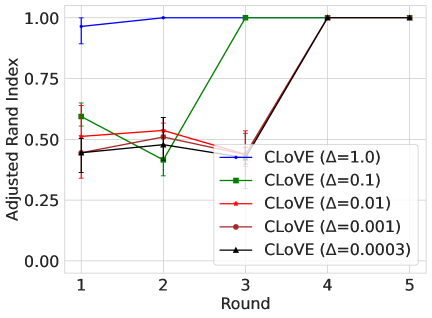
(a) Clustering accuracy of CLoVE over time (rounds) for different values of $\Delta$

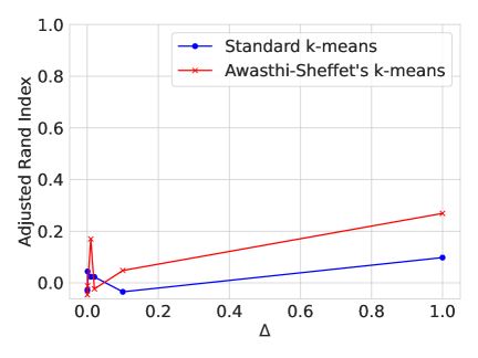
(b) Clustering accuracy of k-FED using standard k-means vs with awasthi2012improved ’s enhancements

Figure 3: Linear regression experiment results

As shown, CLoVE consistently recovers the correct cluster assignment. Moreover, as expected, the convergence rate of CLoVE slows down when the optimal model parameters are closer together (i.e. when $\Delta$ is smaller). In contrast, the performance of k-FED Dennis_2021 on the same data, even with Awasthi-Sheffet’s k-means enhancements awasthi2012improved , is significantly worse (Fig. 3(b)). This discrepancy can be attributed to the fact that the cluster centers (i.e. the mean of their data) are very close to the origin, highlighting the limitations of k-FED in such scenarios. Our results demonstrate that CLoVE outperforms k-FED, especially when the cluster centers are not well-separated.

C.1.2 Additional label skews

Table 7 presents image classification test accuracy results for MNIST, FMNIST, CIFAR-10 datasets on additional types of label skews. The corresponding ARI accuracy results are presented in Table 8 and the clustering convergence results in Table 9. These results include two cases Label skew 3 and Label skew 4. The case Label skew 3 is a data distribution in which there is significant overlap between labels assigned to clients of different clusters. Specifically, there are 5 clusters with 5 clients each. Among the first 4 clusters, all clients of a cluster get samples from all 10 classes except one. The missing class is uniquely selected for each of the 4 clusters. The clients of the 5th cluster get samples from all 10 classes. The case Label skew 4 is a data distribution in which $s\%$ of data (we use one third) for clients belonging to a cluster is uniformly sampled from all classes, and the remaining $(100-s)\%$ comes from a dominant class that is unique for each cluster xu_personalized_2023_FedPAC . Each cluster has 5 clients each of which is assigned 500 samples. For both the Label skew 3 and Label skew 4 cases the data of a class is distributed amongst the clients that are assigned that class by sampling from a Dirichlet distribution with parameter $\alpha=0.5$.

Table 7: Supervised test accuracy results for MNIST, CIFAR-10 and FMNIST

Data mixing	Algorithm	MNIST	CIFAR-10	FMNIST
Label skew 3	FedAvg	$\mathbf{99.0\pm 0.0}$	$\mathbf{84.1\pm 0.5}$	$\mathbf{88.8\pm 0.3}$
	Local-only	$85.9\pm 0.6$	$41.1\pm 1.5$	$71.1\pm 0.4$
	Per-FedAvg	$95.3\pm 0.3$	$41.6\pm 0.7$	$74.9\pm 0.7$
	FedProto	$88.8\pm 0.2$	$39.9\pm 0.4$	$74.1\pm 0.2$
	FedALA	$94.7\pm 0.3$	$40.0\pm 0.7$	$75.1\pm 0.5$
	FedPAC	$95.6\pm 0.2$	$41.4\pm 0.6$	$75.5\pm 0.8$
	CFL	$97.9\pm 0.1$	$61.2\pm 0.6$	$84.3\pm 1.2$
	FeSEM	$94.0\pm 0.2$	$13.3\pm 0.2$	$72.2\pm 1.9$
	FlexCFL	$92.2\pm 0.3$	$20.8\pm 0.5$	$79.7\pm 0.5$
	PACFL	$82.8\pm 0.9$	$27.1\pm 3.8$	$68.1\pm 2.1$
	IFCA	$94.2\pm 0.2$	$57.3\pm 1.9$	$80.6\pm 1.0$
	CLoVE	$94.2\pm 0.2$	$56.9\pm 0.5$	$79.5\pm 0.5$
Label skew 4	FedAvg	$\mathbf{98.5\pm 0.1}$	$60.7\pm 0.8$	$85.9\pm 0.2$
	Local-only	$94.8\pm 0.2$	$67.1\pm 0.5$	$85.5\pm 0.1$
	Per-FedAvg	$95.6\pm 0.1$	$63.7\pm 0.8$	$83.7\pm 0.1$
	FedProto	$93.3\pm 0.2$	$45.3\pm 0.7$	$76.5\pm 0.3$
	FedALA	$96.8\pm 0.1$	$69.8\pm 0.3$	$87.3\pm 0.1$
	FedPAC	$96.1\pm 0.2$	$66.3\pm 0.5$	$84.8\pm 0.3$
	CFL	$97.8\pm 0.1$	$71.3\pm 1.1$	$88.2\pm 0.4$
	FeSEM	$94.9\pm 0.3$	$11.9\pm 1.5$	$80.6\pm 1.1$
	FlexCFL	$97.2\pm 0.1$	$66.8\pm 0.0$	$89.5\pm 0.1$
	PACFL	$93.4\pm 0.2$	$67.4\pm 0.3$	$84.1\pm 0.2$
	IFCA	$98.0\pm 0.1$	$64.3\pm 0.9$	$89.4\pm 0.2$
	CLoVE	$97.8\pm 0.2$	$\mathbf{72.6\pm 0.3}$	$\mathbf{89.9\pm 0.1}$

Table 8: Supervised ARI results for MNIST, CIFAR-10 and FMNIST

Data mixing	Algorithm	MNIST	CIFAR-10	FMNIST
Label skew 3	CFL	$0.00\pm 0.00$	$0.77\pm 0.18$	$0.00\pm 0.00$
	FeSEM	$0.18\pm 0.00$	$0.00\pm 0.00$	$0.00\pm 0.00$
	FlexCFL	$\mathbf{1.00\pm 0.00}$	$\mathbf{1.00\pm 0.00}$	$\mathbf{1.00\pm 0.00}$
	PACFL	$0.20\pm 0.08$	$0.00\pm 0.00$	$0.15\pm 0.13$
	IFCA	$0.92\pm 0.12$	$0.69\pm 0.08$	$0.65\pm 0.15$
	CLoVE	$\mathbf{1.00\pm 0.00}$	$\mathbf{1.00\pm 0.00}$	$\mathbf{1.00\pm 0.00}$
Label skew 4	CFL	$0.00\pm 0.00$	$0.61\pm 0.03$	$0.29\pm 0.02$
	FeSEM	$0.12\pm 0.00$	$0.00\pm 0.00$	$0.11\pm 0.02$
	FlexCFL	$\mathbf{1.00\pm 0.00}$	$\mathbf{1.00\pm 0.00}$	$\mathbf{1.00\pm 0.00}$
	PACFL	$0.53\pm 0.06$	$0.66\pm 0.07$	$0.92\pm 0.02$
	IFCA	$0.55\pm 0.03$	$0.36\pm 0.22$	$0.50\pm 0.05$
	CLoVE	$0.60\pm 0.10$	$\mathbf{1.00\pm 0.00}$	$0.95\pm 0.07$

Table 9: Convergence behavior for MNIST, CIFAR-10 and FMNIST

Data mixing	Algorithm	% of final ARI reached in 10 rounds			First round when ARI $\geq 90\%$
		MNIST	CIFAR-10	FMNIST	MNIST	CIFAR-10	FMNIST
Label skew 2	CFL	$0.0\pm 0.0$	$0.0\pm 0.0$	$0.0\pm 0.0$	—	$48.0\pm 12.0$	$25.3\pm 1.9$
	FeSEM	$\mathbf{100.0\pm 0.0}$	$0.0\pm 0.0$	$0.0\pm 0.0$	$\mathbf{1.0\pm 0.0}$	—	—
	FlexCFL	$\mathbf{100.0\pm 0.0}$	$\mathbf{100.0\pm 0.0}$	$\mathbf{100.0\pm 0.0}$	$\mathbf{1.0\pm 0.0}$	$\mathbf{1.0\pm 0.0}$	$\mathbf{1.0\pm 0.0}$
	PACFL	$\mathbf{100.0\pm 0.0}$	$\mathbf{100.0\pm 0.0}$	$\mathbf{100.0\pm 0.0}$	$\mathbf{1.0\pm 0.0}$	$\mathbf{1.0\pm 0.0}$	$\mathbf{1.0\pm 0.0}$
	IFCA	$\mathbf{100.0\pm 0.0}$	$90.7\pm 13.2$	$\mathbf{100.0\pm 0.0}$	$2.0\pm 0.0$	$19.7\pm 25.0$	$3.3\pm 1.2$
	CLoVE	$\mathbf{100.0\pm 0.0}$	$\mathbf{100.0\pm 0.0}$	$\mathbf{100.0\pm 0.0}$	$2.0\pm 0.0$	$2.0\pm 0.0$	$2.0\pm 0.0$
Label skew 3	CFL	$0.0\pm 0.0$	$0.0\pm 0.0$	$0.0\pm 0.0$	—	$65.7\pm 2.5$	—
	FeSEM	$\mathbf{100.0\pm 0.0}$	$0.0\pm 0.0$	$0.0\pm 0.0$	$\mathbf{1.0\pm 0.0}$	—	—
	FlexCFL	$\mathbf{100.0\pm 0.0}$	$\mathbf{100.0\pm 0.0}$	$\mathbf{100.0\pm 0.0}$	$\mathbf{1.0\pm 0.0}$	$\mathbf{1.0\pm 0.0}$	$\mathbf{1.0\pm 0.0}$
	PACFL	$\mathbf{100.0\pm 0.0}$	$0.0\pm 0.0$	$\mathbf{100.0\pm 0.0}$	$\mathbf{1.0\pm 0.0}$	—	$\mathbf{1.0\pm 0.0}$
	IFCA	$\mathbf{100.0\pm 0.0}$	$\mathbf{100.0\pm 0.0}$	$\mathbf{100.0\pm 0.0}$	$2.0\pm 0.0$	$2.0\pm 0.0$	$3.3\pm 0.5$
	CLoVE	$\mathbf{100.0\pm 0.0}$	$\mathbf{100.0\pm 0.0}$	$\mathbf{100.0\pm 0.0}$	$2.0\pm 0.0$	$2.0\pm 0.0$	$2.0\pm 0.0$
Label skew 4	CFL	$0.0\pm 0.0$	$0.0\pm 0.0$	$0.0\pm 0.0$	—	$50.0\pm 20.5$	$22.0\pm 0.0$
	FeSEM	$\mathbf{100.0\pm 0.0}$	$0.0\pm 0.0$	$\mathbf{100.0\pm 0.0}$	$\mathbf{1.0\pm 0.0}$	—	$\mathbf{1.0\pm 0.0}$
	FlexCFL	$\mathbf{100.0\pm 0.0}$	$\mathbf{100.0\pm 0.0}$	$\mathbf{100.0\pm 0.0}$	$\mathbf{1.0\pm 0.0}$	$\mathbf{1.0\pm 0.0}$	$\mathbf{1.0\pm 0.0}$
	PACFL	$\mathbf{100.0\pm 0.0}$	$\mathbf{100.0\pm 0.0}$	$\mathbf{100.0\pm 0.0}$	$\mathbf{1.0\pm 0.0}$	$\mathbf{1.0\pm 0.0}$	$\mathbf{1.0\pm 0.0}$
	IFCA	$97.6\pm 3.4$	$\mathbf{100.0\pm 0.0}$	$\mathbf{100.0\pm 0.0}$	$2.0\pm 0.0$	$2.3\pm 0.5$	$2.0\pm 0.0$
	CLoVE	$\mathbf{100.0\pm 0.0}$	$\mathbf{100.0\pm 0.0}$	$\mathbf{100.0\pm 0.0}$	$2.0\pm 0.0$	$2.0\pm 0.0$	$2.0\pm 0.0$
Feature skew	CFL	$0.0\pm 0.0$	$0.0\pm 0.0$	$0.0\pm 0.0$	$21.0\pm 0.0$	$85.0\pm 2.9$	$73.7\pm 37.2$
	FeSEM	$0.0\pm 0.0$	$0.0\pm 0.0$	$0.0\pm 0.0$	—	—	—
	FlexCFL	$\mathbf{100.0\pm 0.0}$	$\mathbf{100.0\pm 0.0}$	$\mathbf{100.0\pm 0.0}$	$\mathbf{\mathbf{1.0\pm 0.0}}$	$\mathbf{1.0\pm 0.0}$	$\mathbf{1.0\pm 0.0}$
	PACFL	$0.0\pm 0.0$	$0.0\pm 0.0$	$\mathbf{100.0\pm 0.0}$	—	—	$\mathbf{1.0\pm 0.0}$
	IFCA	$\mathbf{100.0\pm 0.0}$	$\mathbf{100.0\pm 0.0}$	$\mathbf{100.0\pm 0.0}$	$2.7\pm 0.5$	$3.7\pm 0.9$	$3.3\pm 0.5$
	CLoVE	$\mathbf{100.0\pm 0.0}$	$\mathbf{100.0\pm 0.0}$	$\mathbf{100.0\pm 0.0}$	$2.0\pm 0.0$	$4.3\pm 0.9$	$2.0\pm 0.0$

C.1.3 Additional details for text classification

The ARI accuracy and speed of convergence results for the Amazon Review and AG News datasets are presented in Table 10 and Table 11, respectively.

Table 10: Supervised ARI results for Amazon Review and AG News

Algorithm	Amazon Review	AG News
CFL	$0.07\pm 0.08$	$0.39\pm 0.07$
FeSEM	$0.00\pm 0.01$	$0.14\pm 0.00$
FlexCFL	$0.00\pm 0.02$	$0.02\pm 0.00$
PACFL	$0.00\pm 0.00$	$0.00\pm 0.00$
IFCA	$0.29\pm 0.20$	$0.64\pm 0.12$
CLoVE	$\mathbf{0.73\pm 0.24}$	$\mathbf{0.94\pm 0.09}$

Table 11: Convergence behavior for the Amazon Review and AG News datasets

Algorithm	% of final ARI reached in 10 rounds		First round when ARI $\geq 90\%$
	Amazon	AG News	Amazon	AG News
CFL	$0.0\pm 0.0$	$0.0\pm 0.0$	$24.3\pm 4.0$	$38.0\pm 9.1$
FeSEM	$66.7\pm 47.1$	$\mathbf{100.0\pm 0.0}$	$34.0\pm 46.7$	$\mathbf{1.0\pm 0.0}$
FlexCFL	$66.7\pm 47.1$	$\mathbf{100.0\pm 0.0}$	$34.0\pm 46.7$	$\mathbf{1.0\pm 0.0}$
PACFL	$0.0\pm 0.0$	$0.0\pm 0.0$	—	—
IFCA	$\mathbf{100.0\pm 0.0}$	$\mathbf{100.0\pm 0.0}$	$\mathbf{2.7\pm 0.5}$	$2.7\pm 0.5$
CLoVE	$89.0\pm 15.6$	$\mathbf{100.0\pm 0.0}$	$8.3\pm 8.3$	$2.0\pm 0.0$

C.2 Additional unsupervised results

For this section’s experiments, we have used a batch size of 64.

C.2.1 Benefit of personalization

We now examine the reconstruction loss performance of the trained models and show the benefit of our personalized models over traditional FL models. For MNIST and $K=10$, $m=5$ and $n=250$, we run 4 different algorithms: CLoVE, IFCA, FedAvg, Local-only. In FedAvg, i.e. the original FL algorithm, a single model is trained and aggregated by all clients, regardless of their true cluster (equivalently, FedAvg is CLoVE with $K=1$). Local-only means federated models but no aggregation: each client trains its own model only on its local data, and does not share it with the rest of the system.

For this experiment, we consider that each of the 50 clients has a testset of the same data class of the client’s trainset, and we feed its testset through all models (10 models for CLoVE and IFCA, 1 for FedAvg and 50 for Local-only), creating the loss matrices shown as heatmaps in Fig. 4 (run for a single seed value). The vertical axis represents clients, one selected from each true cluster, and the horizontal represents the different models. Clients and models are labeled so that the diagonal represents the true client to model/cluster assignment. Numbers on the heatmap express the reconstruction loss (multiplied by a constant for the sake of presentation) for each client testset and model combination. Very high values are hidden and the corresponding cells are colored red. For the local case, we only show 10 of the 50 models, the ones that correspond to the selected clients.

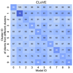
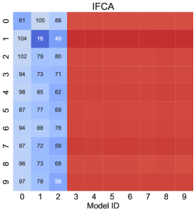
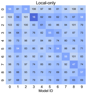
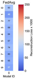
Figure 4: Heatmaps of reconstruction loss of MNIST digits by models clustered and trained by each algorithm

We observe that in all cases, the reconstruction loss of each client’s assigned model by CLoVE (the diagonal) is the smallest in the client’s row (i.e. the smallest among all models), which confirms that the models CLoVE assigned to each client are actually trained to reconstruct the client’s data (MNIST digit) well, and not reconstruct well the other digits. On the contrary, IFCA gets stuck and assigns all clients to 3 clusters (models) – the first 3 columns. The rest of the models remain practically untouched (untrained), hence their high (red) loss values on all clients’ data. The 3 chosen models are not good for the reconstruction of MNIST digits, because they don’t achieve the lowest loss on their respective digits.

Comparing CLoVE and FedAvg, we see that for each row (client from each cluster), the loss achieved by CLoVE is lower than that achieved by FedAvg. This demonstrates the benefit of our personalized FL approach over traditional FL: FedAvg uses a single model to train on local data of each client, and aggregates updated parameters only for this single model. CLoVE, on the other hand, clusters the similar clients together and trains a separate model on the data of clients belonging to each cluster, thus effectively learning – and tailoring the model to – the cluster’s particular data distribution. Finally, comparing CLoVE with Local-only, we see that the diagonal losses achieved by CLoVE on the selected models for each client are lower than the corresponding diagonal losses by Local-only. This shows the benefit of federated learning, as CLoVE models are trained on data from multiple clients from the same cluster, unlike Local-only where clients only train models based on their limited amount of private data.

C.2.2 Scaling with the number of clients

In this experiment, we examine the effect of increasing the number of clients. We use MNIST with $K=10$ clusters and $n=100$ datapoints/client, with $m=10$, 15, 20 clients/cluster. The results are shown in Fig. 5. We observe that for IFCA, the accuracy is bad in both cases, while for CLoVE a higher number of clients leads to faster convergence of the algorithm to the true clusters. This happens because of the larger dimension of the loss vector in the case of more clients, which allows k-means to utilize more loss vector coordinates to distinguish the loss vectors that are similar and should be assigned to the same cluster.

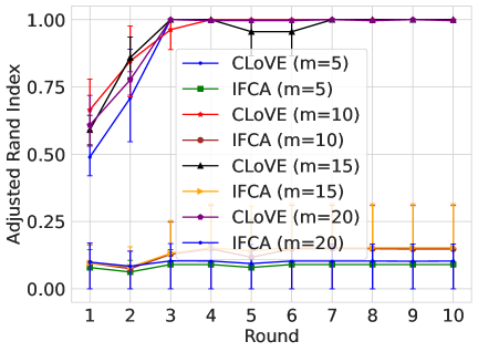
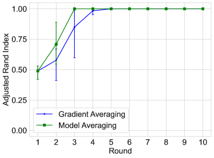
Figure 5: Clustering accuracy of CLoVE and IFCA over time (rounds) for MNIST. Left: For different numbers of clients. Right: For model averaging vs gradient averaging.

C.2.3 Model Averaging versus Gradient Averaging

In this experiment, we compare the two variants of our CLoVE algorithm, i.e. model averaging and gradient averaging. We run an MNIST experiment with $K=10$, $m=5$ and $n=100$, using both averaging methods. The results are shown in Fig. 5. We observe that CLoVE is able to arrive at the correct clustering with both methods, with gradient averaging needing slightly more rounds to do so than model averaging.

C.3 Details on ablation studies

We analyze the impact of changing some of key components of CLoVE one at a time. This includes:

• No Matching: Order the clusters by their smallest client ID and assign models to them in that order (i.e. cluster $k$ gets assigned model $k$). This is in lieu of using the bi-partite matching approach of Alg. 1.

• Agglomerative clustering: Use a different method than k-means to cluster the loss vectors.

• Square root loss: Cluster vectors of square roots of model losses instead of the losses themselves.

Our experiments are for image classification for the CIFAR-10 dataset using 25 clients that are partitioned uniformly among 5 clusters using a label skew with very large overlap. The clients of the first four cluster are assigned samples from every class except one class which is chosen to be different for each cluster. The clients of the fifth cluster are assigned samples from all classes. The partitioning of the data of each class among the clients that are assigned to that class is by sampling from a $\text{Dirichlet}(\alpha)$ distribution with $\alpha=0.5$. The test accuracy achieved is shown in Table 12. We find that “No Matching” has the most impact, as it reduces the test accuracy by almost $4.3\%\pm 1\%$. Switching to Agglomerative clustering results in improvement in the mean test accuracy, but the result is not statistically significant. Likewise, square root loss results in no significant change in performance. This shows that CLoVE is mostly robust in its design.

Table 12: Ablation studies

	Test accuracy
Original CLoVE	$58.3\pm 1.4$
No matching	$55.8\pm 0.6$
Agglomerative clustering	$59.3\pm 1.5$
Square root loss	$58.1\pm 3.3$

References

- (1) B. McMahan, E. Moore, D. Ramage, S. Hampson, and B. A. y Arcas, “Communication-Efficient Learning of Deep Networks from Decentralized Data,” in Proceedings of the 20th International Conference on Artificial Intelligence and Statistics, ser. Proceedings of Machine Learning Research, A. Singh and J. Zhu, Eds., vol. 54. PMLR, Apr. 2017, pp. 1273–1282. [Online]. Available: https://proceedings.mlr.press/v54/mcmahan17a.html
- (2) J. Konečný, H. B. McMahan, F. X. Yu, P. Richtarik, A. T. Suresh, and D. Bacon, “Federated Learning: Strategies for Improving Communication Efficiency,” in NIPS Workshop on Private Multi-Party Machine Learning, 2016. [Online]. Available: https://arxiv.org/abs/1610.05492
- (3) K. Bonawitz, H. Eichner, W. Grieskamp, D. Huba, A. Ingerman, V. Ivanov, C. Kiddon, J. Konecny, S. Mazzocchi, H. McMahan et al., “Towards Federated Learning at Scale: System Design,” in Proceedings of the 2nd SysML Conference, 2019, pp. 1–15.
- (4) A. Sefidcon, C. Vulkán, and M. Gruber, “UNEXT – A unified networking experience,” Nokia Bell Labs, Technical Report, 2023. [Online]. Available: https://www.nokia.com/asset/213573
- (5) Y. Zhao, M. Li, L. Lai, N. Suda, D. Civin, and V. Chandra, “Federated Learning with Non-IID Data,” in arXiv preprint arXiv:1806.00582, 2018, pp. 1–10.
- (6) A. Z. Tan, H. Yu, L. Cui, and Q. Yang, “Towards Personalized Federated Learning,” IEEE Transactions on Neural Networks and Learning Systems, vol. 34, no. 12, pp. 9587–9603, 2023.
- (7) F. Hanzely and P. Richtárik, “Federated Learning of a Mixture of Global and Local Models,” arXiv preprint arXiv:2002.05516, 2020.
- (8) A. Ghosh, J. Chung, D. Yin, and K. Ramchandran, “An Efficient Framework for Clustered Federated Learning,” in Proceedings of the 34th International Conference on Neural Information Processing Systems, ser. NIPS ’20. Red Hook, NY, USA: Curran Associates Inc., Dec. 2020, pp. 19 586–19 597.
- (9) M. Werner, L. He, M. Jordan, M. Jaggi, and S. P. Karimireddy, “Provably Personalized and Robust Federated Learning,” Transactions on Machine Learning Research, Aug. 2023. [Online]. Available: https://openreview.net/forum?id=B0uBSSUy0G
- (10) F. Sattler, K.-R. Müller, and W. Samek, “Clustered Federated Learning: Model-Agnostic Distributed Multitask Optimization Under Privacy Constraints,” IEEE Transactions on Neural Networks and Learning Systems, vol. 32, no. 8, pp. 3710–3722, Aug. 2021, conference Name: IEEE Transactions on Neural Networks and Learning Systems.
- (11) Y. Mansour, M. Mohri, J. Ro, and A. T. Suresh, “Three Approaches for Personalization with Applications to Federated Learning,” Jul. 2020. [Online]. Available: http://arxiv.org/abs/2002.10619
- (12) J. Chung, K. Lee, and K. Ramchandran, “Federated Unsupervised Clustering with Generative Models,” in AAAI 2022 international workshop on trustable, verifiable and auditable federated learning, vol. 4, 2022.
- (13) G. Long, M. Xie, T. Shen, T. Zhou, X. Wang, and J. Jiang, “Multi-Center Federated Learning: Clients Clustering for Better Personalization,” World Wide Web, vol. 26, no. 1, pp. 481–500, Jan. 2023. [Online]. Available: https://doi.org/10.1007/s11280-022-01046-x
- (14) M. Duan, D. Liu, X. Ji, Y. Wu, L. Liang, X. Chen, Y. Tan, and A. Ren, “Flexible Clustered Federated Learning for Client-Level Data Distribution Shift,” IEEE Transactions on Parallel and Distributed Systems, vol. 33, no. 11, pp. 2661–2674, Nov. 2022. [Online]. Available: https://ieeexplore.ieee.org/document/9647969
- (15) S. Vahidian, M. Morafah, W. Wang, V. Kungurtsev, C. Chen, M. Shah, and B. Lin, “Efficient Distribution Similarity Identification in Clustered Federated Learning via Principal Angles between Client Data Subspaces,” Proceedings of the AAAI Conference on Artificial Intelligence, vol. 37, no. 8, pp. 10 043–10 052, Jun. 2023, number: 8. [Online]. Available: https://ojs.aaai.org/index.php/AAAI/article/view/26197
- (16) P. Awasthi and O. Sheffet, “Improved Spectral-Norm Bounds for Clustering,” in International Workshop on Approximation Algorithms for Combinatorial Optimization. Springer, 2012, pp. 37–49.
- (17) A. Kumar and R. Kannan, “Clustering with Spectral Norm and the k-means Algorithm,” in 2010 IEEE 51st Annual Symposium on Foundations of Computer Science. IEEE, 2010, pp. 299–308.
- (18) D. Treder-Tschechlov, “k-Means Clustering on Image Data using the MNIST Dataset,” 2024, accessed: 2025-01-29. [Online]. Available: https://medium.com/@tschechd/k-means-clustering-on-image-data-using-the-mnist-dataset-8101fcc650eb
- (19) D. K. Dennis, T. Li, and V. Smith, “Heterogeneity for the Win: One-Shot Federated Clustering,” in Proceedings of the 38th International Conference on Machine Learning. PMLR, Jul. 2021, pp. 2611–2620, iSSN: 2640-3498. [Online]. Available: https://proceedings.mlr.press/v139/dennis21a.html
- (20) X. Yi, C. Caramanis, and S. Sanghavi, “Alternating Minimization for Mixed Linear Regression,” in International Conference on Machine Learning. PMLR, 2014, pp. 613–621.
- (21) X. Li, K. Huang, W. Yang, S. Wang, and Z. Zhang, “On the Convergence of FedAvg on Non-IID Data,” arXiv preprint arXiv:1907.02189, 2019.
- (22) A. Fallah, A. Mokhtari, and A. Ozdaglar, “Personalized Federated Learning with Theoretical Guarantees: A Model-Agnostic Meta-Learning Approach,” in Proceedings of the 34th International Conference on Neural Information Processing Systems, ser. NIPS ’20. Red Hook, NY, USA: Curran Associates Inc., Dec. 2020, pp. 3557–3568.
- (23) J. Zhang, Y. Hua, H. Wang, T. Song, Z. Xue, R. Ma, and H. Guan, “FedALA: Adaptive Local Aggregation for Personalized Federated Learning,” Proceedings of the AAAI Conference on Artificial Intelligence, vol. 37, no. 9, pp. 11 237–11 244, Jun. 2023, number: 9. [Online]. Available: https://ojs.aaai.org/index.php/AAAI/article/view/26330
- (24) Y. Jiang, J. Konečný, K. Rush, and S. Kannan, “Improving Federated Learning Personalization via Model Agnostic Meta Learning,” 2023. [Online]. Available: https://arxiv.org/abs/1909.12488
- (25) V. Smith, C.-K. Chiang, M. Sanjabi, and A. S. Talwalkar, “Federated Multi-Task Learning,” in Advances in Neural Information Processing Systems, I. Guyon, U. V. Luxburg, S. Bengio, H. Wallach, R. Fergus, S. Vishwanathan, and R. Garnett, Eds., vol. 30. Curran Associates, Inc., 2017. [Online]. Available: https://proceedings.neurips.cc/paper_files/paper/2017/file/6211080fa89981f66b1a0c9d55c61d0f-Paper.pdf
- (26) J. Xu, X. Tong, and S.-L. Huang, “Personalized Federated Learning with Feature Alignment and Classifier Collaboration,” in The Eleventh International Conference on Learning Representations, 2023. [Online]. Available: https://openreview.net/forum?id=SXZr8aDKia
- (27) Y. Deng, M. M. Kamani, and M. Mahdavi, “Adaptive Personalized Federated Learning,” arXiv preprint arXiv:2003.13461, 2020.
- (28) Y. Mansour, M. Mohri, J. Ro, and A. T. Suresh, “Three Approaches for Personalized Federated Learning,” in Advances in Neural Information Processing Systems, 2020, pp. 1–13.
- (29) H. Kim, H. Kim, and G. De Veciana, “Clustered Federated Learning via Gradient-based Partitioning,” in Proceedings of the 41st International Conference on Machine Learning, ser. ICML’24. JMLR.org, 2024.
- (30) Y. Tan, G. Long, L. Liu, T. Zhou, Q. Lu, J. Jiang, and C. Zhang, “FedProto: Federated Prototype Learning across Heterogeneous Clients,” Proceedings of the AAAI Conference on Artificial Intelligence, vol. 36, no. 8, pp. 8432–8440, Jun. 2022, number: 8. [Online]. Available: https://ojs.aaai.org/index.php/AAAI/article/view/20819
- (31) Z. Chen, H. H. Yang, T. Q. Quek, and K. F. E. Chong, “Spectral Co-Distillation for Personalized Federated Learning,” in Proceedings of the 37th International Conference on Neural Information Processing Systems, ser. NIPS ’23. Red Hook, NY, USA: Curran Associates Inc., Dec. 2023, pp. 8757–8773.
- (32) H. Vardhan, A. Ghosh, and A. Mazumdar, “An Improved Federated Clustering Algorithm with Model-based Clustering,” Transactions on Machine Learning Research, 2024. [Online]. Available: https://openreview.net/forum?id=1ZGA5mSkoB
- (33) D. P. Kingma and J. Ba, “Adam: A Method for Stochastic Optimization,” Jan. 2017, arXiv:1412.6980 [cs]. [Online]. Available: http://arxiv.org/abs/1412.6980
- (34) A. Ghosh, J. Chung, D. Yin, and K. Ramchandran, “An Efficient Framework for Clustered Federated Learning,” IEEE Transactions on Information Theory, vol. 68, no. 12, pp. 8076–8091, Dec. 2022. [Online]. Available: https://ieeexplore.ieee.org/document/9832954
- (35) A. Dasgupta, J. Hopcroft, R. Kannan, and P. Mitra, “Spectral Clustering with Limited Independence,” in Proceedings of the eighteenth annual ACM-SIAM symposium on Discrete algorithms. Citeseer, 2007, pp. 1036–1045.
- (36) B. Laurent and P. Massart, “Adaptive Estimation of a Quadratic Functional by Model Selection,” Annals of statistics, pp. 1302–1338, 2000.
- (37) M. J. Wainwright, High-Dimensional Statistics: A Non-Asymptotic Viewpoint, ser. Cambridge Series in Statistical and Probabilistic Mathematics. Cambridge University Press, 2019.
- (38) Y. LeCun, L. Bottou, Y. Bengio, and P. Haffner, “Gradient-based Learning Applied to Document Recognition,” Proceedings of the IEEE, vol. 86, no. 11, pp. 2278–2324, Nov. 1998, conference Name: Proceedings of the IEEE. [Online]. Available: https://ieeexplore.ieee.org/document/726791
- (39) A. Krizhevsky, “Learning Multiple Layers of Features from Tiny Images,” Toronto, ON, Canada, 2009. [Online]. Available: https://www.cs.toronto.edu/˜kriz/cifar.html
- (40) H. Xiao, K. Rasul, and R. Vollgraf, “Fashion-MNIST: A Novel Image Dataset for Benchmarking Machine Learning Algorithms,” Sep. 2017, arXiv:1708.07747 [cs]. [Online]. Available: http://arxiv.org/abs/1708.07747
- (41) J. Ni, J. Li, and J. McAuley, “Justifying Recommendations using Distantly-Labeled Reviews and Fine-Grained Aspects,” in Proceedings of the 2019 Conference on Empirical Methods in Natural Language Processing and the 9th International Joint Conference on Natural Language Processing (EMNLP-IJCNLP), K. Inui, J. Jiang, V. Ng, and X. Wan, Eds. Hong Kong, China: Association for Computational Linguistics, Nov. 2019, pp. 188–197. [Online]. Available: https://aclanthology.org/D19-1018/
- (42) A. Gulli, “AG’s Corpus of News Articles.” [Online]. Available: http://groups.di.unipi.it/˜gulli/AG_corpus_of_news_articles.html
- (43) X. Zhang, J. Zhao, and Y. LeCun, “Character-level Convolutional Networks for Text Classification,” in Advances in Neural Information Processing Systems, vol. 28. Curran Associates, Inc., 2015. [Online]. Available: https://papers.nips.cc/paper_files/paper/2015/hash/250cf8b51c773f3f8dc8b4be867a9a02-Abstract.html
- (44) A. Paszke, S. Gross, F. Massa, A. Lerer, J. Bradbury, G. Chanan, T. Killeen, Z. Lin, N. Gimelshein, L. Antiga, A. Desmaison, A. Köpf, E. Yang, Z. DeVito, M. Raison, A. Tejani, S. Chilamkurthy, B. Steiner, L. Fang, J. Bai, and S. Chintala, “PyTorch: An Imperative Style, High-Performance Deep Learning Library,” in Proceedings of the 33rd International Conference on Neural Information Processing Systems. Red Hook, NY, USA: Curran Associates Inc., Dec. 2019, no. 721, pp. 8026–8037.