Quantum-geometric dipole: a topological boost to flavor ferromagnetism in flat bands

Abstract

Robust flavor-polarized phases are a striking hallmark of many flat-band moiré materials. In this work, we trace the origin of this spontaneous polarization to a previously overlooked quantum-geometric quantity: the quantum-geometric dipole. Analogous to how the quantum metric governs the spatial spread of wavepackets, we show that the quantum-geometric dipole sets the characteristic size of particle-hole excitations, e.g. magnons in a ferromagnet, which in turn boosts their gap and stiffness. Indeed, the larger the particle-hole separation, the weaker the mutual attraction, and the stronger the excitation energy. In topological bands, this energy enhancement admits a lower bound within the single-mode approximation, highlighting the crucial role of topology in flat-band ferromagnetism. We illustrate these effects in microscopic models, emphasizing their generality and relevance to moiré materials. Our results establish the quantum-geometric dipole as a predictive geometric indicator for ferromagnetism in flat bands, a crucial prerequisite for topological order.

Introduction —

Quantum geometry provides a lens to understand contributions to macroscopic observables—such as conductivity, polarizability, or optical responses—that elude semiclassical explanations because they arise from how quantum states are “sewn” together [1, 2, 3, 4]. To quantify this sewing, a family of quantum geometric quantities has been introduced. The most useful among them share two key features: (i) they are related to physical observables, e.g. the quantum metric sets a bound on Wannier localization [5] and governs the spin stiffness in flat-band superconductors [6]; and ($ii$) they possess predictive power, offering material design principles when combined with topology [7, 8, 9, 10, 11, 12, 13, 14, 15, 16, 17, 18].

In this work, we promote the quantum-geometric dipole to the status of a core quantum-geometric quantity alongside the Berry curvature and quantum metric. Originally introduced in the context of excitonic photoresponses [19, 20, 21, 22, 23, 24], we refine and extend the concept to show that it satisfies both criteria outlined above. Specifically, we first recall that it measures the typical separation between the particle ($p$) and hole ($h$) in a $ph$ excitation (Fig. 1a) [25, 26]; we then relate it to the gap and stiffness of such excitations (Fig. 1b); and finally show that topological invariants impose approximate lower bounds on these quantities, which become exact for flat ideal bands [27, 28, 29, 30, 31, 32, 33, 34, 35], within the single-mode approximation.

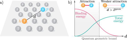
Figure 1: a) Schematics of the magnon dipole ${\bm{d}}$ measuring the distance between the $\downarrow$-particle ($p$, blue) and $\uparrow$-hole ($h$, orange) forming the flavor-flipping excitation. b) As the average dipole increases, the attraction between the oppositely charged $p$ and $h$ weakens, which decreases the magnon’s binding energy (red) and increases its total energy (green) – see Eq. 5. The quantum-geometric dipole $\mathcal{S}^{\rm geom}$ sets the typical amplitude of the magnon dipole, resulting in larger magnon energies (non-shaded area) that can be lower bounded up to $\mathcal{O}(1)$ factors by topological invariants – see Eqs. 8 and 9.

The relation between the $ph$ excitation energy and dipole strength admits a simple physical interpretation: as the dipole grows, the oppositely charged $p$ and $h$ become more spatially separated, their mutual attraction weakens, and the total energy of the excitation rises. The topological lower bound we derive for the $ph$ energy mirrors that of the Wannier function spread from the quantum metric [36]: just as the quantum metric measures the average spread of an electron around its center of mass, and is bounded below (up to an $\mathcal{O}(1)$ factor) by the electronic Chern number [33, 37]; the quantum geometric dipole estimates the $ph$ distance and is similarly bounded by the difference of $p$ and $h$ Chern numbers. This, in turn, results in an approximate topological lower bound on the $ph$ energy via its dependence on the dipole. Our result provides a natural explanation for the widely observed tendency of topological flat bands to spontaneously polarize under interactions [38, 39, 40, 41, 42, 43, 44, 45, 46, 47, 48, 49, 50, 51].

Quantum geometric effects are especially pronounced in flat bands, where semiclassical dynamics vanish and interactions dominate—a regime routinely realized in moiré [52, 53, 54] and other superlattice [55, 56, 57, 58, 59, 60, 61, 62, 63, 64] materials, which host a wide range of correlated and topological phases [65, 66, 67, 68, 69, 70, 71, 72]. For instance, fractionalized topological phases have recently been observed without magnetic fields in twisted MoTe₂ [42, 43, 44, 45] and penta-layer graphene [47, 51]. Crucial to their realization at experimentally accessible temperatures is a robust and spontaneous time-reversal symmetry breaking [73, 74, 75, 76], enabled by extended ferromagnetic phases. Focusing on twisted MoTe₂, we numerically demonstrate that this robustness originates from the quantum-geometric dipole.

By clarifying its fundamental properties and crucial role in stabilizing topologically ordered phases in moiré materials, our work establishes the quantum-geometric dipole as a core quantum-geometric quantity. While our primary focus is on magnons relevant to moiré ferromagnets, the scope of the quantum geometric dipole extends far beyond, providing a finer understanding of interaction-driven phenomena for excitons, superconductors, or multiband systems.

Quantum geometric dipole —

The central object of our study is the magnon electric dipole, i.e. the distance between the particle and hole forming the spin-flip excitation. While a similar particle–hole dipole has appeared in the context of excitonic photoresponses [19, 20, 21, 22, 23, 24, 25, 77, 78, 79, 80, 81, 82, 83, 84], our definition clarifies two of its key properties: it separates the quantum-geometric contribution from the non-universal spatial part; and it recasts the quantum-geometric part as a Berry-like flux in mixed spin–momentum space, which offers an efficient, gauge-invariant, and numerically-stable expression à la Fukui-Hatsugai [85, 86] (Eq. 3 below).

To set the stage, consider a generic band with dispersion $\varepsilon_{\bm{k},\sigma}$ and periodic Bloch states $|u_{k}^{\sigma}\rangle$ annihilated by $c_{\bm{k},\sigma}$, with $\bm{k}$ in the Brillouin zone (BZ) and $\sigma\in\{\uparrow,\downarrow\}$ a flavor index. While our treatment extends to any band filling, we focus on the half-filled case and study magnons created over the ferromagnetic state $|\hskip-3.0pt\Uparrow\rangle=\prod_{\bm{k}\in{\rm BZ}}c_{\bm{k},\uparrow}^{\dagger}|\varnothing\rangle$ with $|\varnothing\rangle$ the vacuum. For $|\hskip-4.0pt\Uparrow\rangle$ to be an eigenstate, we require (at least) U(1)-flavor symmetry, i.e. that the Hamiltonian be diagonal in $\sigma$. A generic band-projected flavor-flipping excitation with momentum $\bm{Q}$ can be written as

$$\begin{split}|\psi_{\bm{Q}}\rangle&=\frac{1}{\sqrt{N_{\bm{Q}}}}\sum_{\bm{k}\in{\rm BZ}}\psi_{\bm{Q},\bm{k}}c_{\bm{k}+\bm{Q}/2,\downarrow}^{\dagger}c_{\bm{k}-\bm{Q}/2,\uparrow}|\!\Uparrow\rangle,\\ \psi_{\bm{Q},\bm{k}}&=z_{\bm{Q},\bm{k}}s_{\bm{Q},\bm{k}},\quad s_{\bm{Q},\bm{k}}=\langle u_{\bm{k}+\bm{Q}/2}^{\downarrow}|u_{\bm{k}-\bm{Q}/2}^{\uparrow}\rangle,\end{split}$$ (1)

with $N_{\bm{Q}}=\sum_{\bm{k}\in\text{BZ}}|\psi_{\bm{Q},\bm{k}}|^{2}$ a normalization factor, and where we have decomposed the wavefunction coefficients into a gauge-invariant component $z_{\bm{Q},\bm{k}}$ capturing the spatial structure of the magnon, and a spin-flipping form factor $s_{\bm{Q},\bm{k}}$ originating from band projection.

With these notations, the magnon electric dipole ${\bm{d}}$, defined as the average distance between the spin-$\downarrow$ particle and spin-$\uparrow$ hole, takes the form (see Ref. [25] or supplemental material (SM) Sec. A)

$${\bm{d}}=\left\langle\mathcal{S}_{\bm{Q},\bm{k}}^{\rm spat}+\mathcal{S}_{\bm{Q},\bm{k}}^{\rm geom}\right\rangle_{|\psi_{\bm{Q}}|^{2}},\quad\mathcal{S}_{\bm{Q},\bm{k}}^{\rm spat}=i\nabla_{\bm{k}}\log z_{\bm{Q},\bm{k}},$$

$$\mathcal{S}_{\bm{Q},\bm{k}}^{\rm geom}=\mathcal{A}_{\bm{k}-\bm{Q}/2}^{\uparrow}-\mathcal{A}_{\bm{k}+\bm{Q}/2}^{\downarrow}+i\nabla_{\bm{k}}\log s_{\bm{Q},\bm{k}},$$ (2)

with $\mathcal{A}_{\bm{k}}^{\sigma}=-i\langle u_{\bm{k},\sigma}|\nabla_{\bm{k}}|u_{\bm{k},\sigma}\rangle$ the spin-resolved Berry connection, and where $\langle O_{\bm{k}}\rangle_{\mu}=\sum_{\bm{k}}\mu_{\bm{k}}O_{\bm{k}}/\sum_{\bm{k}}\mu_{\bm{k}}$ denotes the $\mu$-weighted average. We have isolated two contributions to the magnon dipole. The first, dubbed the spatial dipole and denoted as $\mathcal{S}^{\rm spat}$, only depends on the $z$-coefficients and therefore originates from the structure of the dipole in real space. The second, $\mathcal{S}^{\rm geom}$, is the quantum-geometric dipole advertised in the introduction. It is manifestly gauge-invariant , and depends solely on the Bloch vectors of the underlying bands.

To emphasize the spatial/geometric characters of the two terms in Eq. 2, consider the following two limits. When the Bloch bundle is geometrically trivial, $|u_{\bm{k}}^{\sigma}\rangle=1$, $\mathcal{S}^{\rm geom}$ vanishes and the $ph$ dipole entirely comes from the spatial part $\mathcal{S}^{\rm spat}$. On the other hand, the most localized magnon with center-of-mass momentum $\bm{Q}$, given by $\int{\rm d}^{2}\bm{R}\,e^{i(\bm{Q}\cdot\bm{R})}c_{\bm{R},\downarrow}^{\dagger}c_{\bm{R},\uparrow}|\!\Uparrow\rangle$, corresponds to $z_{\bm{Q},\bm{k}}=1$ after projection, leading to $\mathcal{S}^{\rm spat}=0$ and a purely quantum-geometric dipole $\bm{d}=\langle\mathcal{S}^{\rm geom}_{\bm{k}}\rangle_{|\psi|^{2}}$.

Beyond these two limits, the geometric character of $\mathcal{S}^{\rm geom}$ becomes clear when interpreted as a Berry-like flux. To unveil it, we discretize the BZ in steps of $\delta\bm{k}_{a}=|\delta k|{\bm{b}}_{a}$ along the reciprocal lattice vectors ${\bm{b}}_{a=1,2}$ and approximate derivatives by finite differences to obtain at lowest order in $|\delta k|$

$$\delta\bm{k}_{a}\cdot\mathcal{S}_{\bm{Q},\bm{k}}^{\rm geom}=i\log\left[\frac{\Lambda_{\bm{k}}^{\uparrow}(\delta\bm{k}_{a})}{\Lambda_{\bm{k}}^{\downarrow}(\delta\bm{k}_{a})}\frac{s_{\bm{Q},\bm{k}+\delta\bm{k}_{a}}}{s_{\bm{Q},\bm{k}}}\right],\;\leavevmode\hbox to71.01pt{\vbox to64.4pt{\text{[drawing]}}} \uparrow \downarrow k+\delta k_{a} k \delta k_{a}\cdot\mathcal{S}_{Q,k}^{\rm geom}$$ (3)

where $\Lambda_{\bm{k}}^{\sigma}(\bm{q})=\langle u_{\bm{k}+\bm{q}-\sigma\frac{\bm{Q}}{2}}^{\sigma}|u_{\bm{k}-\sigma\frac{\bm{Q}}{2}}^{\sigma}\rangle$ are spin-resolved form factors. The arrows on the accompanying sketch represent link variables [85, 86] corresponding to the terms in the logarithm (for $\bm{Q}=0$). The closed loop they form emphasizes the gauge invariance of our discretized expression and its interpretation as a Berry flux – or quantum geometric curvature in mixed spin-momentum.

Magnon interaction energy —

In the introduction, we argued that the interaction-induced magnon gap should scale with the amplitude of the magnon dipole, ${\bm{d}}$: a larger dipole means more separation between the spin-$\downarrow$ particle and spin-$\uparrow$ hole, which reduces their mutual attraction and thereby increases the overall magnon energy. To rationalize this intuition, we compute $\Delta(\psi_{\bm{Q}})=\langle\psi_{\bm{Q}}|H_{\rm int}|\psi_{\bm{Q}}\rangle-\langle\Uparrow\hskip-5.0pt|H_{\rm int}|\hskip-5.0pt\Uparrow\rangle$, the interaction energy of the magnon relative to the ferromagnetic state for a band-projected interaction $H_{\rm int}=\sum_{\begin{subarray}{c}\bm{q},\bm{k},\bm{p}\\ \sigma,\tau\end{subarray}}\frac{v(q)}{2N_{\rm BZ}}\langle u_{\bm{k}+\bm{q}}^{\sigma}|u_{\bm{k}}^{\sigma}\rangle\langle u_{\bm{p}}^{\tau}|u_{\bm{p}+\bm{q}}^{\tau}\rangle c_{\bm{k}+\bm{q},\sigma}^{\dagger}c_{\bm{p},\tau}^{\dagger}c_{\bm{p}+\bm{q},\tau}c_{\bm{k},\sigma}$, with $N_{\rm BZ}$ the number of points in the discretized BZ, and $v(q=||\bm{q}||)$ a rotation-symmetric Coulomb potential. Wick’s theorem yields (see SM Sec. B)

$$\Delta(\psi)=\left\langle\sum_{\bm{q}}\frac{v(q)|\Lambda_{\bm{k}}^{\uparrow}(\bm{q})|^{2}}{N_{\rm BZ}}\left[1-\frac{\Lambda_{\bm{k}}^{\downarrow}(\bm{q})^{*}}{\Lambda_{\bm{k}}^{\uparrow}(\bm{q})^{*}}\frac{\psi_{\bm{k}+\bm{q}}}{\psi_{\bm{k}}}\right]\right\rangle_{\!\!|\psi|^{2}}\!\!\!\!\!,$$ (4)

where we have left the $\bm{Q}$ dependence implicit. The total energy of the magnon also includes a kinetic term $K(\psi_{\bm{Q}})=\left\langle\varepsilon_{\bm{k}+\bm{Q}/2,\downarrow}-\varepsilon_{\bm{k}-\bm{Q}/2,\uparrow}\right\rangle_{|\psi_{\bm{Q}}|^{2}}$. The stability of the state $|\hskip-3.0pt\Uparrow\rangle$ against magnonic excitations requires that the Stoner criterion, $\min_{z_{\bm{Q}}}[K(\psi_{\bm{Q}})+\Delta(\psi_{\bm{Q}})]>0$, be fulfilled at all $\bm{Q}$. For flat bands in which the bandwidth is negligible compared to the interaction scale, we can safely ignore $K(\psi)$.

The connection between the interaction gap $\Delta(\psi)$ and the quantum-geometric dipole is brought to light by a small-$\bm{q}$ expansion of the form factors — a standard approach for identifying geometric contributions to physical observables [88, 89, 90, 91, 92, 93, 94, 95]. The zeroth order term in the expansion vanishes since the bracketed terms in Eq. 4 cancel out ($\Lambda_{\bm{k}}^{\sigma}(0)=1$). The linear terms also vanish due to the rotation invariance of $v(q)$. Hence, the leading contribution is of order $q^{2}$, which, by dimensional analysis, requires the introduction of a typical length scale. One may deduce this length scale should be the magnon’s dipole by recalling that $\psi_{\bm{k}}\propto s_{\bm{k}}$ and observing that the phase of the bracketed term in Eq. 4 is precisely the spin-momentum Berry flux sketched in Eq. 3 up to the replacement $\delta\bm{k}_{a}\to\bm{q}$. Confirming this intuition, the complete expansion (detailed in SM Sec. B) yields

$$\Delta(\psi)=a^{-2}\left\langle U(g_{\bm{k}})\left[||\mathcal{S}_{\bm{k}}^{\rm geom}+\mathcal{S}_{\bm{k}}^{\rm spat}||^{2}\right]\right\rangle_{|\psi|^{2}},$$ (5)

with $a$ the lattice constant. In this calculation, the decay of the form factors for large-$\bm{q}$ (not captured by the small-$\bm{q}$ expansion) is enforced by re-exponentiating the terms proportional to the quantum metric $(g_{\bm{k}}^{\sigma})^{ab}={\rm Re}\,\langle\partial_{k_{a}}u_{\bm{k}}^{\sigma}|\partial_{k_{b}}u_{\bm{k}}^{\sigma}\rangle-\mathcal{A}_{\bm{k},a}^{\sigma}\mathcal{A}_{\bm{k},b}^{\sigma}$. Considering these effective momentum cutoffs as independent of spin, we obtain the momentum-dependent interaction scale $U(g_{\bm{k}})=(4N_{\rm BZ})^{-1}\sum_{\bm{q}}(qa)^{2}v(q)e^{-q_{a}g^{ab}_{\bm{k}}q_{b}}$ with $g_{\bm{k}}=(g_{\bm{k}}^{\uparrow}+g_{\bm{k}}^{\downarrow})/2$ the spin-averaged quantum metric. This coefficient has an intuitive interpretation: it describes the typical repulsion between two oppositely charged Gaussian wavepackets of width $g_{\bm{k}}$, the minimal spread allowed by the band’s quantum geometry. To see this, let us momentarily specialize to the two-body Coulomb potential $v(\bm{r})=e^{2}/(4\pi\varepsilon|\bm{r}|)$ and assume an isotropic quantum metric with $\tilde{g}={\rm Tr}g$; then

$$U(g)=\frac{\pi e^{2}a^{2}}{\varepsilon(8\pi\tilde{g})^{3/2}}=\frac{\pi a^{2}}{8}\int{\rm d}^{2}\bm{r}\,v(\bm{r})|\phi(\bm{r})|^{4},$$ (6)

with $\phi(\bm{r})=\exp(-\bm{r}^{2}/2\tilde{g})/\sqrt{2\pi\tilde{g}}$ a normalized Gaussian wavepacket, and where $a^{2}$ is required by dimensionality. Eq. 5 confirms the intuitive idea that the magnon energy grows with its dipole.

Furthermore, within the single-mode approximation (SMA), the magnon gap is entirely determined by the quantum-geometric dipole. Specifically, the SMA assumes that to decrease the total dipole, the lowest energy magnons are well described by projecting local-in-space spin-flips of the form $c_{\bm{R},\downarrow}^{\dagger}c_{\bm{R},\uparrow}|\!\Uparrow\rangle$, i.e. setting $z_{\bm{k}}=1$, so that $\psi_{\bm{k}}=s_{\bm{k}}$. This choice eliminates the spatial dipole (see discussion above Eq. 3) and isolates the geometric contribution

$$\Delta^{\text{geom}}_{\bm{Q}}=a^{-2}\left\langle U(g_{\bm{k}})||\mathcal{S}_{\bm{Q},\bm{k}}^{\rm geom}||^{2}\right\rangle_{|s|^{2}},$$ (7)

after the small-$\bm{q}$ expansion.

Topological boost to flat-band ferromagnetism —

Having derived the precise relation between the magnon energy and quantum-geometric dipole in flat bands (Eq. 5), we now describe how topology underpins robust ferromagnetism in topological flat bands.

Let us start with the SU(2)-spin invariant limit $|u_{\bm{k},\uparrow}\rangle=|u_{\bm{k},\downarrow}\rangle$, where a gapless magnon branch with quadratic dispersion must exist [96, 97, 98, 99]. We recover this gaplessness by noting that $\mathcal{S}_{\bm{Q}=0,\bm{k}}^{\rm geom}=0$ for SU(2) invariant systems (see Eq. 2). Turning to Eq. 5, Taylor expanding $\Delta_{\bm{Q}}^{\rm geom}\simeq\rho_{s}|\bm{Q}|^{2}/2$ gives a magnon stiffness $\rho_{s}=\left\langle U(g_{\bm{k}})\Omega_{\bm{k}}^{2}\right\rangle_{\rm BZ}$ with $\Omega_{\bm{k}}=\nabla_{\bm{k}}\times\mathcal{A}_{\bm{k}}^{\uparrow/\downarrow}$ the Berry curvature of the band (see SM Sec. C). When fluctuations of the quantum metric about its mean, $\bar{g}$, can be ignored, this formula reduces to

$$\rho_{s}\simeq U(\bar{g})\langle\Omega_{\bm{k}}^{2}\rangle\geq U(\bar{g})C^{2},$$ (8)

with $C=\langle\Omega_{\bm{k}}\rangle_{\rm BZ}$ the Chern number, and where the inequality follows from Cauchy-Schwarz. This topologically induced lower bound on the spin stiffness qualitatively agrees with previous results [89], and becomes exact for bands with uniform quantum metric [28]. It is derived assuming SU(2) symmetry, but is only non-trivial when the Chern number is non-vanishing. Thus, it is not useful when opposite spins are related by time reversal symmetry, but yields a nontrivial bound in, e.g. valleys of moiré materials away from time-reversal invariant momenta, such as the $K$ valley of twisted bilayer graphene.

We now consider a flavor-symmetry lower than SU(2), for which the magnon spectrum is gapped. We lower bound the magnon gap by a sum of $|C_{s}|$ strictly positive contributions, with $C_{s}=C_{\uparrow}-C_{\downarrow}$ the spin Chern number of the underlying bands. This again highlights the role of topology in flat-band ferromagnetism.

The lower bound arises because the spin-lowering overlap $s_{\bm{Q},\bm{k}}=\langle u_{\bm{k}+\bm{Q}/2}^{\downarrow}|u_{\bm{k}-\bm{Q}/2}^{\uparrow}\rangle$ is a complex function in $\bm{k}$ whose phase needs to increase by $2\pi C_{s}$ as $\bm{k}$ winds around the BZ. It hence possesses at least $|C_{s}|$ vortices at momenta $\{\bm{k}_{v}\}$ with vorticity $\tau={\rm sign}\,C_{s}$ (counted without multiplicities), and can be factorized as $s_{\bm{Q},\bm{k}}=\tilde{s}_{\bm{Q},\bm{k}}\prod_{v}(k^{\tau}-k_{v}^{\tau})$ with $k^{\tau}=k_{x}+i\tau k_{y}$ and $\tilde{s}$ a complex function with no winding. Near these vortices, the quantum-geometric dipole in Eq. 2 is dominated by the singular connection $i\nabla\log s_{\bm{Q}}$ [25], which diverges as $||S_{\bm{Q}}^{\rm geom}||\sim|s_{\bm{Q}}|^{-1}$ when $s_{\bm{Q}}\to 0$. Isolating these singular contributions from the BZ average in Eq. 7, we obtain

$$\Delta_{\bm{Q}}^{\text{geom}}\geq\sum_{v}U(g_{\bm{k}_{v}})\simeq|C_{s}|U(\bar{g}),$$ (9)

where the second (approximate) equality holds under the assumption of a near-uniform quantum metric.

The approximate topological bounds derived for the magnon stiffness (Eq. 8) and gap (Eq. 9) show the fundamental role of topology on the stability of ferromagnetism in flat bands. They arose from the tight connection between the quantum-geometric dipole and the magnon spectrum (Eq. 5). They are consistent with the familiar structure of spin excitations in topologically trivial models, such as the Hubbard model, where a spin-flip can be localized to a single point, which forces the quantum-geometric dipole to vanish and leads to a vanishing gap. This gaplessness in the flat-band limit implies that any additional term in the Hamiltonian (e.g. super-exchange) can dominate, favoring different spin-ordering at low temperature (e.g. antiferromagnetic).

Figure 2: Magnon gap versus $M/A$ for the 2D BHZ model, shown in units of $U_{0}$. The magnon gap is plotted using three different methods: the Bethe–Salpeter analysis (SM Eq. S17, blue); the single-mode approximation (Eq. 4, orange); and the geometric contribution formula (Eq. 7, red), with $z_{\bm{k}}=1$ in the latter two. The shaded blue (red) regions correspond to topological phases with Chern number $C=1$ ($C=-1$) for spin-$\uparrow$. The inset shows $d_{\rm min}^{2}=\langle||\mathcal{S}^{\mathrm{geom}}_{\bm{k}}||^{2}\rangle_{|s|^{2}}$, the average squared quantum-geometric dipole.
Parameters: $A=1$, $B=1$, and $r_{\xi}=0.1$.

Microscopic verification and relevance —

We now substantiate our theory by studying two microscopic models. We focus on systems that break SU(2) but preserve U(1) spin symmetry and compute the magnon gap at $\bm{Q}=0$, where the magnon spectrum attains its minimum. To assess the validity of previous approximations, we compute in Figs. 2 and 3 the magnon energy of two different models using methods of decreasing rigor: the Bethe–Salpeter analysis (SM Eq. S17, blue); the SMA before small-$\bm{q}$ expansion (Eq. 4, orange); and the geometric contribution formula (Eq. 7, red), with $z_{\bm{k}}=1$ in the latter two. To highlight the quantitative relationship between these energies and the quantum-geometric dipole (Fig. 1), we also evaluate $d_{\rm min}^{2}=\langle||\mathcal{S}^{\mathrm{geom}}_{\bm{k}}||^{2}\rangle_{|s|^{2}}$ (shown in insets). These quantities are presented for two representative models. First, we consider the 2D BHZ model [100] and show that the magnon gap is strong in the topological regime and sharply decreases to a near-zero value upon entering the trivial regime, which qualitatively corroborates the effect of topology identified in Eq. 9. Next, we apply our framework to twisted bilayer $\mathrm{MoTe_{2}}$, where spin-valley polarized phases have been observed [41, 42]. At filling $\nu=1$, our coarse Stoner criterion predicts a transition to an unpolarized phase at an interlayer displacement field that closely matches experimental observations, highlighting the predictive power of our method.

$\bullet$ Lattice toy model: The noninteracting part of the 2D BHZ model reads $H_{0}=\mathrm{diag}[\mathcal{H}^{\uparrow},\mathcal{H}^{\downarrow}]$, where $\mathcal{H}^{\sigma}=\big{(}M-2B(2-\cos k_{x}-\cos k_{y})\big{)}\sigma_{z}+A\sigma\sin k_{x}\sigma_{x}+A\sin k_{y}\sigma_{y}$. Choosing $A=B=1$, the model is symmetric around $M=4$ and undergoes topological phase transitions at $M=0,4$ and $8$ at which the Chern number shifts as $C_{\uparrow}=0\to 1\to-1\to 0$ (see SM Sec. D). We then project the screened Coulomb interaction, $v(\bm{q})=\frac{U_{0}}{r_{\xi}|\bm{q}|}\tanh(r_{\xi}|\bm{q}|)$, onto the lower band and neglect the kinetic energy to isolate interaction effects. Fig. 2 shows the magnon gap computed using all three methods at $r_{\xi}=0.1$.

Two striking behaviors emerge from this plot. First, the average squared geometric dipole $d_{\rm min}^{2}$ evolves with the same trend as the magnon gap. This supports the physical picture developed in Fig. 1 and formalized in Eq. 7 that a greater dipole, or spatial separation between the spin-$\uparrow$ and spin-$\downarrow$ forming the magnon, correlates with the ferromagnetic gap. Second, we notice that the ferromagnetic gap is finite across the topological region of the phase diagram, peaking near the $C=1\to-1$ transition at $M=4$, but sharply diminishes upon entering the trivial phase. This underscores the crucial role of topology in stabilizing ferromagnetic order by enhancing the average quantum-geometric dipole, as explained in Eq. 9 and surrounding text.

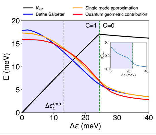
Figure 3: Same as Fig. 2 for the continuum model of $\theta$-twisted bilayer MoTe₂. Gray dashed line marks the transition from polarized to unpolarized phases, $\Delta\varepsilon_{c}^{\rm exp}\approx 13~{\rm meV}$, extracted from the MCD measurements of Ref. [42]. Using a relaxed Stoner criterion, our theory estimates the transition point to occur at around $\Delta\varepsilon_{c}^{\rm th}\approx 16-17~{\rm meV}$, corresponding to the crossing points between the maximal kinetic energy gain $K_{\rm kin}=\max(|\varepsilon_{\bm{k},\downarrow}-\varepsilon_{\bm{k},\uparrow}|)$ (black line) and the magnon interaction energy (colored lines).
Parameters: $\theta=3.7^{\circ}$, $\xi=30~\mathrm{nm}$, $\epsilon=7$, and $\xi_{0}=0.7~\mathrm{nm}$.

$\bullet$ Relevance to moiré materials: To explore the interplay between topology and interaction in realistic systems, we turn to twisted bilayer $\mathrm{MoTe_{2}}$, where experiments have identified a broad, cone-shaped region of spin-valley polarization in the phase diagram spanned by electron filling and displacement field [41]. A stable spin-valley polarized phase is a prerequisite for realizing exotic correlated states [73], in particular for the fractional Chern insulator recently observed in this system [42].

We focus on the case of filling $\nu=1$ at a twist angle of $\theta=3.7^{\circ}$, using the continuum moiré Hamiltonian (details in SM Sec. D) [101, 102, 103, 104]. An important tunable parameter is the interlayer displacement field $D$, which creates an interlayer potential difference $\Delta\varepsilon=\frac{eD}{\epsilon\epsilon_{0}}\xi_{0}$ with $\xi_{0}$ the interlayer spacing and $\epsilon$ the dielectric constant. The long-range Coulomb interaction is screened by dual metal gates, resulting in an effective potential of the form $v(\bm{q})=\frac{e^{2}}{2\epsilon_{0}\epsilon}\frac{\tanh(\xi|\bm{q}|)}{|\bm{q}|}$, where $\xi$ is the distance from the bilayer to the gates. We adopt representative experimental parameters: $\xi=30~\mathrm{nm}$, $\epsilon=7$, and $\xi_{0}=0.7~\mathrm{nm}$.

Fig. 3 presents the magnon gap versus interlayer displacement potential, and demonstrates a remarkable agreement among the three methods discussed above. Similar to the BHZ model, the difference between the topological and trivial regimes is stark: the magnon interaction energy drops to less than one-third of its initial value at $\Delta\varepsilon=0$ upon crossing the topological transition indicated by the vertical green dashed line.

Experimentally, a transition from a ferromagnetic to an unpolarized phase is observed as a function of increasing displacement field, which we estimate around $\Delta\varepsilon_{c}^{\rm exp}\approx 13~$meV (gray dashed line) using Ref. [42]’s data. To evaluate this transition point theoretically, we employ a relaxed Stoner criterion by approximating the kinetic contribution to the magnon energy as $K_{\rm kin}=\max(|\varepsilon_{\bm{k},\downarrow}-\varepsilon_{\bm{k},\uparrow}|)$, shown as the black solid line in Fig. 3, an upper bound on the kinetic energy cost $K(\psi)$ defined above. The ferromagnetic transition is expected to occur at the intersection between the kinetic energy cost and the magnon gap. This occurs around $\Delta\varepsilon_{c}^{\rm th}=16-17~{\rm meV}$ for all three methods used in Fig. 3, which closely matches $\Delta\varepsilon_{c}^{\rm exp}$.

These two microscopic examples underscore the central role of the quantum-geometric dipole in the emergence of ferromagnetism. They support our approximate topological lower bound, which accounts for the widely observed tendency of topological bands to spontaneously polarize under interactions. Moreover, the strong agreement between our predictions and the depolarization transition point in twisted MoTe₂ highlights the quantitative accuracy and predictive power of our approach.

Acknowledgments —

VC is indebted to C. Paiva for an insightful presentation of her results [25] while the manuscript was being written. We also acknowledge insightful conversations with S. Divic and M. Goerbig. LC, SAAG and JC acknowledge support from the Air Force Office of Scientific Research under Grants No. FA9550-20-1-0260 and FA9550-24-1-0222. SAAG and JC acknowledge support from the Alfred P. Sloan Foundation through a Sloan Research Fellowship. The Flatiron Institute is a division of the Simons Foundation.

Supplemental Material

Contents

1. A Quantum geometric dipole
2. B Magnon gap and quantum geometric dipole
   1. 1 Bethe-Salpeter formula and spin-flip spectrum
   2. 2 Single mode approximation
   3. 3 Relation between magnon gap and quantum geometric dipole
3. C Magnon spin stiffness
4. D Microscopic models
   1. 1 Interacting BHZ model
   2. 2 tMoTe₂ and ferromagnetism

A Quantum geometric dipole

In this appendix, we derive Eq. 2 of the main text by providing the real-space representation of the magnon wavefunction (Eq. 1) and computing the average distance between the hole and electron that form this excitation.

Real-space representation: We consider a system whose ground state is a fully polarized ferromagnet, denoted by $|\Uparrow\rangle=\prod_{\bm{k}\in{\rm BZ}}c^{\dagger}_{\bm{k},\uparrow}|\varnothing\rangle$ as defined in the main text. Let us denote the operator annihilating a fermion of spin $\sigma$ at position $\bm{r}$ as $c_{\bm{r},\sigma}$, whose real-space orbital is a delta function at position $\bm{r}$, and write $|\bm{r}_{\downarrow},\bm{r}_{\uparrow}\rangle=c_{\bm{r}_{\downarrow},\downarrow}^{\dagger}c_{\bm{r}_{\uparrow},\uparrow}|\Uparrow\rangle$. Recalling that the $c_{\bm{k},\sigma}$ operators used in the main text are the fermionic operator for a specific band corresponding to the eigenstates $e^{i\bm{k}\cdot\bm{r}}|u_{\bm{k}}^{\sigma}\rangle$, and that the anti-commutation relation between fermionic operators is equal to the scalar product of their respective orbitals, it follows that $\{c_{\bm{r},\sigma},c_{\bm{k},\sigma^{\prime}}^{\dagger}\}=\delta_{\sigma,\sigma^{\prime}}\langle\bm{r}|u_{\bm{k}}^{\sigma}\rangle e^{i\bm{k}\cdot\bm{r}}$ where $\langle\bm{r}|u_{\bm{k}}^{\sigma}\rangle$ denotes the real-space representation of the periodic function $|u_{\bm{k}}^{\sigma}\rangle$. For convenience, we repeat here the generic band-projected magnon state introduced in the main text:

$$|\psi_{\bm{Q}}\rangle=\frac{1}{\sqrt{N_{\bm{Q}}}}\sum_{\bm{k}\in{\rm BZ}}\psi_{\bm{Q},\bm{k}}\underbrace{c_{\bm{k}+\bm{Q}/2,\downarrow}^{\dagger}c_{\bm{k}-\bm{Q}/2,\uparrow}|\Uparrow\rangle}_{|S_{\bm{Q},\bm{k}}^{-}\rangle},\quad\psi_{\bm{Q},\bm{k}}=z_{\bm{Q},\bm{k}}s_{\bm{Q},\bm{k}},\quad s_{\bm{Q},\bm{k}},=\langle u_{\bm{k}+\bm{Q}/2}^{\downarrow}|u_{\bm{k}-\bm{Q}/2}^{\uparrow}\rangle,$$ (S1)

with $N_{\bm{Q}}=\sum_{\bm{k}\in\text{BZ}}|\psi_{\bm{Q},\bm{k}}|^{2}$ a normalization factor. This state can be expressed in real-space as

$$\langle\bm{r}_{\downarrow},\bm{r}_{\uparrow}|\psi_{\bm{Q}}\rangle =\sum_{\bm{k}\in{\rm BZ}}\frac{\psi_{\bm{Q},\bm{k}}}{\sqrt{N_{\bm{Q}}}}\langle\Uparrow|c_{\bm{r}_{\uparrow},\uparrow}^{\dagger}c_{\bm{r}_{\downarrow},\downarrow}c_{\bm{k}+\bm{Q}/2,\downarrow}^{\dagger}c_{\bm{k}-\bm{Q}/2,\uparrow}|\Uparrow\rangle$$ (S2)

$$=\sum_{\bm{k}\in{\rm BZ}}\frac{\psi_{\bm{Q},\bm{k}}}{\sqrt{N_{\bm{Q}}}}e^{i(\bm{k}\cdot\bm{r}+\bm{Q}\cdot\bm{R})}\langle\bm{r}_{\downarrow}|u_{\bm{k}+\frac{\bm{Q}}{2}}^{\downarrow}\rangle\langle\bm{r}_{\uparrow}|u_{\bm{k}-\frac{\bm{Q}}{2}}^{\uparrow}\rangle^{*},\quad\bm{R}=\frac{\bm{r}_{\uparrow}+\bm{r}_{\downarrow}}{2},\quad\bm{r}=\bm{r}_{\downarrow}-\bm{r}_{\uparrow},$$ (S3)

where we have used the anti-commutation relation discussed above, and introduced the center of mass $\bm{R}$ and relative $\bm{r}$ coordinates.

Average particle-hole dipole: Reproducing the calculation from Ref. [25] for completeness, we can now compute the expectation value of the relative distance as

$$\bm{d} =\langle\psi|\bm{r}|\psi\rangle=\int{\rm d}^{2}\bm{r}_{\downarrow}{\rm d}^{2}\bm{r}_{\uparrow}\,\langle\psi|\bm{r}_{\downarrow},\bm{r}_{\uparrow}\rangle\bm{r}\langle\bm{r}_{\downarrow},\bm{r}_{\uparrow}|\psi\rangle$$ (S4)

$$=\frac{1}{N}\sum_{\bm{k},\bm{k}^{\prime}}\int{\rm d}^{2}\bm{r}_{\downarrow}{\rm d}^{2}\bm{r}_{\uparrow}\,\psi_{\bm{k}^{\prime}}^{*}\psi_{\bm{k}}\langle u_{\bm{k}^{\prime}+\frac{\bm{Q}}{2},\downarrow}|\bm{r}_{\downarrow}\rangle\langle\bm{r}_{\uparrow}|u_{\bm{k}^{\prime}-\frac{\bm{Q}}{2},\uparrow}\rangle\langle\bm{r}_{\downarrow}|u_{\bm{k}+\frac{\bm{Q}}{2},\downarrow}\rangle\langle u_{\bm{k}-\frac{\bm{Q}}{2},\uparrow}|\bm{r}_{\uparrow}\rangle e^{-i(\bm{k}^{\prime}\cdot\bm{r})}\bm{r}e^{i(\bm{k}\cdot\bm{r})}$$ (S5)

$$=\frac{1}{N}\sum_{\bm{k},\bm{k}^{\prime}}\int{\rm d}^{2}\bm{r}_{\downarrow}{\rm d}^{2}\bm{r}_{\uparrow}\,\psi_{\bm{k}^{\prime}}^{*}\psi_{\bm{k}}\langle u_{\bm{k}^{\prime}+\frac{\bm{Q}}{2},\downarrow}|\bm{r}_{\downarrow}\rangle\langle\bm{r}_{\uparrow}|u_{\bm{k}^{\prime}-\frac{\bm{Q}}{2},\uparrow}\rangle\langle\bm{r}_{\downarrow}|u_{\bm{k}+\frac{\bm{Q}}{2},\downarrow}\rangle\langle u_{\bm{k}-\frac{\bm{Q}}{2},\uparrow}|\bm{r}_{\uparrow}\rangle e^{-i(\bm{k}^{\prime}\cdot\bm{r})}(-i\nabla_{\bm{k}})e^{i(\bm{k}\cdot\bm{r})}$$ (S6)

$$=\frac{1}{N}\sum_{\bm{k},\bm{k}^{\prime}}\int{\rm d}^{2}\bm{r}_{\downarrow}{\rm d}^{2}\bm{r}_{\uparrow}\,\psi_{\bm{k}^{\prime}}^{*}\langle u_{\bm{k}^{\prime}+\frac{\bm{Q}}{2},\downarrow}|\bm{r}_{\downarrow}\rangle\langle\bm{r}_{\uparrow}|u_{\bm{k}^{\prime}-\frac{\bm{Q}}{2},\uparrow}\rangle e^{i(\bm{k}\cdot\bm{r}-\bm{k}^{\prime}\cdot\bm{r})}(i\nabla_{\bm{k}})\left[\psi_{\bm{k}}\langle\bm{r}_{\downarrow}|u_{\bm{k}+\frac{\bm{Q}}{2},\downarrow}\rangle\langle\bm{r}_{\uparrow}|u_{\bm{k}-\frac{\bm{Q}}{2},\uparrow}\rangle^{*}\right]$$ (S7)

$$=\frac{i}{N}\sum_{\bm{k},\bm{k}^{\prime}}\psi_{\bm{k}}^{*}\mathcal{O}_{\bm{k}-\bm{k}^{\prime}}(u_{\bm{k}^{\prime}+\bm{Q}/2}^{\downarrow},u_{\bm{k}+\bm{Q}/2}^{\downarrow})\mathcal{O}_{\bm{k}^{\prime}-\bm{k}}(u_{\bm{k}-\bm{Q}/2}^{\uparrow},u_{\bm{k}^{\prime}-\bm{Q}/2}^{\uparrow})\nabla_{\bm{k}}\psi_{\bm{k}}$$

$$\qquad+\frac{i}{N}\sum_{\bm{k},\bm{k}^{\prime}}|\psi_{\bm{k}}|^{2}\mathcal{O}_{\bm{k}-\bm{k}^{\prime}}(u_{\bm{k}^{\prime}+\bm{Q}/2}^{\downarrow},\nabla_{\bm{k}}u_{\bm{k}+\bm{Q}/2}^{\downarrow})\mathcal{O}_{\bm{k}^{\prime}-\bm{k}}(u_{\bm{k}-\bm{Q}/2}^{\uparrow},u_{\bm{k}^{\prime}-\bm{Q}/2}^{\uparrow})$$ (S8)

$$\qquad+\frac{i}{N}\sum_{\bm{k},\bm{k}^{\prime}}|\psi_{\bm{k}}|^{2}\mathcal{O}_{\bm{k}-\bm{k}^{\prime}}(u_{\bm{k}^{\prime}+\bm{Q}/2}^{\downarrow},u_{\bm{k}+\bm{Q}/2}^{\downarrow})\mathcal{O}_{\bm{k}^{\prime}-\bm{k}}(\nabla_{\bm{k}}u_{\bm{k}-\bm{Q}/2}^{\uparrow},u_{\bm{k}^{\prime}-\bm{Q}/2}^{\uparrow}),$$

where we have used integration by parts between lines Eq. S6 and Eq. S7, and have also defined the overlap $\mathcal{O}_{\bm{q}}(\phi_{1},\phi_{2})=\int{\rm d}^{2}\bm{r}\langle\phi_{2}|\bm{r}\rangle e^{i\bm{r}\cdot\bm{q}}\langle\bm{r}|\phi_{1}\rangle$ between any unit-cell periodic functions $\phi_{1,2}$. Because the periodic functions carry no crystal momentum, it must be that $\mathcal{O}_{\bm{q}}(\phi_{1},\phi_{2})\propto\delta_{\bm{q}}$. Then the resolution of the identity yields $\mathcal{O}_{\bm{q}}(\phi_{1},\phi_{2})=\delta_{\bm{q}}\langle\phi_{2}|(\int{\rm d}^{2}\bm{r}|\bm{r}\rangle\langle\bm{r}|)|\phi_{1}\rangle=\delta_{\bm{q}}\langle\phi_{2}|\phi_{1}\rangle$. This gives

$$\bm{d} =\frac{i}{N}\sum_{\bm{k}}\psi_{\bm{k}}^{*}\nabla_{\bm{k}}\psi_{\bm{k}}+|\psi_{\bm{k}}|^{2}\left[\langle u_{\bm{k}+\frac{\bm{Q}}{2},\downarrow}|\nabla_{\bm{k}}u_{\bm{k}+\frac{\bm{Q}}{2},\downarrow}\rangle+\langle\nabla_{\bm{k}}u_{\bm{k}-\frac{\bm{Q}}{2},\uparrow}|u_{\bm{k}-\frac{\bm{Q}}{2},\uparrow}\rangle\right]$$ (S9)

$$=\frac{i}{N}\sum_{\bm{k}}\psi_{\bm{k}}^{*}\nabla_{\bm{k}}\psi_{\bm{k}}+|\psi_{\bm{k}}|^{2}\left[\langle u_{\bm{k}+\frac{\bm{Q}}{2},\downarrow}|\nabla_{\bm{k}}u_{\bm{k}+\frac{\bm{Q}}{2},\downarrow}\rangle-\langle u_{\bm{k}-\frac{\bm{Q}}{2},\uparrow}|\nabla_{\bm{k}}u_{\bm{k}-\frac{\bm{Q}}{2},\uparrow}\rangle\right]$$ (S10)

$$=\sum_{\bm{k}}\frac{|\psi_{\bm{k}}|^{2}}{N}\left[i\nabla_{\bm{k}}\log z_{\bm{k}}+i\nabla_{\bm{k}}\log s_{\bm{k}}-\mathcal{A}_{\bm{k}+\frac{\bm{Q}}{2}}^{\downarrow}+\mathcal{A}_{\bm{k}-\frac{\bm{Q}}{2}}^{\uparrow}\right]=\sum_{\bm{k}}\frac{|\psi_{\bm{k}}|^{2}}{N}\left[\mathcal{S}^{\rm spat}_{\bm{k}}+\mathcal{S}^{\rm geom}_{\bm{k}}\right],$$ (S11)

where we have omitted the dependence on the center of mass momentum $\bm{Q}$ and used the fact that Bloch vectors are normalized to go from Eq. S9 to Eq. S10. This gives Eq. 2 in the main text.

B Magnon gap and quantum geometric dipole

This appendix contains all details relevant to the numerical simulations presented in Figs. 2 and 3 of the main text, and the key steps necessary to derive our main analytical results (Eqs. 4 - 9). In more details

• Sec. 1 derives the Bethe-Salpeter equation for collective excitations.

• Sec. 2 details the single-mode approximation that provides an analytically tractable approximation of the lowest-lying magnon excitation.

• Sec. 3 performs the small-$\bm{q}$ expansion sketched in the main text and derives the explicit expression linking the magnon gap to the quantum geometric dipole (Eq. 5).

1 Bethe-Salpeter formula and spin-flip spectrum

We start from a generic interacting Hamiltonian projected onto the bands of interest

$$H=H_{0}+H_{\rm int},\quad H_{0}=\sum_{\bm{k},\sigma}\varepsilon_{\bm{k},\sigma}c_{\bm{k},\sigma}^{\dagger}c_{\bm{k},\sigma},\quad H_{\rm int}=\frac{1}{2}\sum_{\bm{k},\bm{p},\bm{q},\sigma\tau}W_{\bm{k}\bm{p}}^{\sigma\tau}(\bm{q})c_{\bm{k}+\bm{q},\sigma}^{\dagger}c_{\bm{p}\tau}^{\dagger}c_{\bm{p}+\bm{q},\tau}c_{\bm{k}\sigma}$$ (S12)

where the interaction matrix elements $W_{\bm{k}\bm{p}}^{\sigma\tau}(\bm{q})$ depend on the band form factors $\Gamma_{\bm{k},\sigma}(\bm{q})=\langle u_{\bm{k}+\bm{q}}^{\sigma}|u_{\bm{k}}^{\sigma}\rangle$ and the Fourier transform of the (rotation invariant) interaction potential $v(q=||\bm{q}||)$ as

$$W^{\sigma\tau}_{\bm{k}\bm{p}}(\bm{q})=\frac{v(\bm{q})}{N_{\rm BZ}}\Gamma_{\bm{k},\sigma}(\bm{q})\Gamma^{*}_{\bm{p},\tau}(\bm{q})=\frac{v(\bm{q})}{N_{\rm BZ}}\langle u_{\bm{k}+\bm{q}}^{\sigma}|u_{\bm{k}}^{\sigma}\rangle\langle u_{\bm{p}}^{\tau}|u_{\bm{p}+\bm{q}}^{\tau}\rangle.$$ (S13)

Project the Hamiltonian onto the magnon basis spanned by $|S_{\bm{Q},\bm{k}}^{-}\rangle$, as introduced in Eq. S1, we have

$$\mathcal{H}_{\bm{k},\bm{k}^{\prime}}(\bm{Q}) =\langle S_{\bm{Q},\bm{k}}^{-}|H_{0}+H_{\rm int}|S_{\bm{Q},\bm{k}^{\prime}}^{-}\rangle-\langle\Uparrow|H_{0}+H_{\rm int}|\Uparrow\rangle\delta_{\mathbf{k},\mathbf{k^{\prime}}}$$ (S14)

$$=(E_{\bm{k}_{+},\downarrow}-E_{\bm{k}_{-},\uparrow})\delta_{\bm{k},\bm{k}^{\prime}}-W^{\uparrow,\downarrow}_{\bm{k}_{-},\bm{k}_{+}}(\bm{k}^{\prime}-\bm{k}),\quad\bm{k}_{\pm}=\bm{k}\pm\bm{Q}/2,$$

where the Hartree-Fock quasiparticle energies are given by

$$E_{\bm{k},\downarrow}=\varepsilon_{\bm{k},\downarrow}+\left[\sum_{\bm{p}}W_{\bm{k}\bm{p}}^{\downarrow\uparrow}(0)\right],\quad E_{\bm{k},\uparrow}=\varepsilon_{\bm{k},\uparrow}+\left[\sum_{\bm{p}}W^{\uparrow\uparrow}_{\bm{k}\bm{p}}(0)-\sum_{\bm{p}}W_{\bm{p}\bm{p}}^{\uparrow\uparrow}(\bm{k}-\bm{p})\right],$$ (S15)

under the assumption that $|\Uparrow\rangle$ is the ground state. Note that $\mathcal{H}$ is diagonal in the center of mass momentum $\bm{Q}$ of the excitation due to translation invariance. Noticing that the $W^{\sigma,\tau}_{\bm{p},\bm{k}}(0)=v(0)$ is independent of spin and momentum, the Hartree terms cancel, so that:

$$E_{\bm{k}_{+},\downarrow}-E_{\bm{k}_{-},\uparrow}=\varepsilon_{\bm{k}_{+},\downarrow}-\varepsilon_{\bm{k}_{-},\uparrow}+\sum_{\bm{p}}W_{\bm{p}\bm{p}}^{\uparrow\uparrow}(\bm{k}_{-}-\bm{p}),$$ (S16)

The magnon spectrum is obtained by diagonalizing $\mathcal{H}_{\bm{k},\bm{k}^{\prime}}(\bm{Q})$, i.e. solving the so-called Bethe-Salpeter equation

$$\mathcal{H}_{\bm{k},\bm{k}^{\prime}}(\bm{Q}){\psi}_{\bm{Q},\bm{k}^{\prime}}=\mathcal{E}(\bm{Q})\psi_{\bm{Q},\bm{k}},$$ (S17)

which yields the collective excitation energies $\mathcal{E}(\bm{Q})$, and provides the coefficients $\psi_{\bm{k},\bm{Q}}$ of the corresponding magnon wavefunctions (Eq. S1). In Figs. 2 and 3, we focus on the spectrum at $\bm{Q}=0$, and extract the magnon gap from the lowest eigenvalue of Eq. S17 (curves labeled “Bethe Salpeter” in Figs. 2 and 3).

2 Single mode approximation

The lowest magnon energy can also be obtained by minimizing the expectation value of $\mathcal{H}$ with respect to the coefficients of the magnon wavefunction (we omit the subscript $\bm{Q}$ for clarity when there is no ambiguity)

$$\mathcal{E}_{\rm min}(\bm{Q})=\min_{\{\psi\}}\Delta(\psi),\quad\Delta(\psi)=\frac{1}{N}\sum_{\bm{k}\bm{k}^{\prime}}\psi_{\bm{k}}^{*}\mathcal{H}_{\bm{k},\bm{k}^{\prime}}(\bm{Q})\psi_{\bm{k}^{\prime}},\quad N=\sum_{\bm{k}}|\psi_{\bm{k}}|^{2}.$$ (S18)

Combing Eqs. S14 – S16 yields $\Delta(\psi)=K+I$, where

$$K =\frac{1}{N}\sum_{\bm{k}}|\psi_{\bm{k}}|^{2}(\varepsilon_{\bm{k}_{+},\downarrow}-\varepsilon_{\bm{k}_{-},\uparrow}),$$ (S19)

$$I =\frac{1}{N}\sum_{\bm{k}}\left[|\psi_{\bm{k}}|^{2}\sum_{\bm{p}}W^{\uparrow,\uparrow}_{\bm{p},\bm{p}}(\bm{k}_{-}-\bm{p})\right]-\frac{1}{N}\sum_{\bm{k}\bm{k}^{\prime}}\left[W^{\uparrow,\downarrow}_{\bm{k}_{-},\bm{k}_{+}}(\bm{k}^{\prime}-\bm{k})\psi_{\bm{k}}^{*}\psi_{\bm{k}^{\prime}}\right]$$ (S20)

and $\bm{k}_{\pm}=\bm{k}\pm\bm{Q}/2$. Here, $K$ captures the kinetic energy from the non-interacting band structure, while all interaction effects are gathered in $I$. The stability of the ferromagnetic ground state against spin-flip excitations requires a Stoner-like criterion $I+K>0$ for any choice of $\psi$ and all momenta $\bm{Q}$. In Fig. 3 of the main text (where we only show $\bm{Q}=0$), we adopt a relaxed version of this criterion by comparing $I$ with the maximal kinetic cost $K_{\rm kin}=\max(|\varepsilon_{\bm{k},\downarrow}-\varepsilon_{\bm{k},\uparrow}|)$, which provides an upper bound of $K$.

In the flat-band limit, $K=0$, and the gap is entirely given by the interaction contribution $I$. Expanding Eq. S20 with the explicit form of the interaction kernel (Eq. S13) and splitting $\psi_{\bm{k}}=z_{\bm{k}}s_{\bm{k}}$ gives

$$\Delta(\psi)=I =\frac{1}{N}\sum_{\bm{k},\bm{q}}\frac{v(\bm{q})}{N_{\rm BZ}}\left[|\psi_{\bm{k}}\langle u_{\bm{k}_{-}+\bm{q}}^{\uparrow}|u_{\bm{k}_{-}}^{\uparrow}\rangle|^{2}-\psi_{\bm{k}}^{*}\psi_{\bm{k}+\bm{q}}\langle u_{\bm{k}_{-}+\bm{q}}^{\uparrow}|u_{\bm{k}_{-}}^{\uparrow}\rangle\langle u_{\bm{k}_{+}}^{\downarrow}|u_{\bm{k}_{+}+\bm{q}}^{\downarrow}\rangle\right],$$ (S21)

$$=\frac{1}{N}\sum_{\bm{k}}|\psi_{\bm{k}}|^{2}\sum_{\bm{q}}\frac{v(\bm{q})|\langle u_{\bm{k}_{-}+\bm{q}}^{\uparrow}|u_{\bm{k}_{-}}^{\uparrow}\rangle|^{2}}{N_{\rm BZ}}\left[1-\frac{\psi_{\bm{k}+\bm{q}}}{\psi_{\bm{k}}}\frac{\langle u_{\bm{k}_{+}}^{\downarrow}|u_{\bm{k}_{+}+\bm{q}}^{\downarrow}\rangle}{\langle u_{\bm{k}_{-}}^{\uparrow}|u_{\bm{k}_{-}+\bm{q}}^{\uparrow}\rangle}\right],$$ (S22)

$$=\frac{1}{N}\sum_{\bm{k}}|\psi_{\bm{k}}|^{2}\sum_{\bm{q}}\frac{v(\bm{q})|\Lambda_{\bm{k}}^{\uparrow}(\bm{q})|^{2}}{N_{\rm BZ}}\left[1-\frac{\psi_{\bm{k}+\bm{q}}}{\psi_{\bm{k}}}\frac{\Lambda_{\bm{k}}^{\downarrow}(\bm{q})^{*}}{\Lambda_{\bm{k}}^{\uparrow}(\bm{q})^{*}}\right],$$ (S23)

where we have used the notation $\Lambda_{\bm{k}}^{\sigma}(\bm{q})=\langle u_{\bm{k}+\bm{q}-\sigma\frac{\bm{Q}}{2}}^{\sigma}|u_{\bm{k}-\sigma\frac{\bm{Q}}{2}}^{\sigma}\rangle$, with $\sigma=\pm 1$ for spin-$\uparrow/\downarrow$ (introduced in the main text) to match the form of Eq. 4.

The single-mode approximation discussed in the main text takes $z_{\bm{k}}=1$, yielding

$$\Delta^{\rm SMA}(\psi)=\frac{1}{N}\sum_{\bm{k}}|s_{\bm{k}}|^{2}\sum_{\bm{q}}\frac{v(\bm{q})|\Lambda_{\bm{k}}^{\uparrow}(\bm{q})|^{2}}{N_{\rm BZ}}\left[1-\frac{s_{\bm{k}+\bm{q}}}{s_{\bm{k}}}\frac{\Lambda_{\bm{k}}^{\downarrow}(\bm{q})^{*}}{\Lambda_{\bm{k}}^{\uparrow}(\bm{q})^{*}}\right],$$ (S24)

which corresponds to the curves labeled “Single mode approximation” in Figs. 2 and 3.

3 Relation between magnon gap and quantum geometric dipole

We further approximate $\Delta(\psi)$ by neglecting large-$\bm{q}$ processes. This is justified because both the form factor magnitudes and the screened Coulomb interaction decay with increasing momentum transfer $\bm{q}$. Specifically, we expand the form factors to second order in $\bm{q}$ to capture the small-$\bm{q}$ behavior, and re-exponentiate the parts that includes the quantum metric to ensure fast decay for large-$\bm{q}$. For instance, the norm of the spin-conserving form factors approximately behaves as

$$|\langle u_{\bm{k}+\bm{q}}^{\sigma}|u_{\bm{k}}^{\sigma}\rangle|^{2} =\langle u_{\bm{k}+\bm{q}}^{\sigma}|u_{\bm{k}}^{\sigma}\rangle\langle u_{\bm{k}}^{\sigma}|u_{\bm{k}+\bm{q}}^{\sigma}\rangle$$ (S25)

$$\approx 1+\frac{q_{a}}{2}\left(\langle\partial_{a}u_{\bm{k}}^{\sigma}|u_{\bm{k}}^{\sigma}\rangle+\langle u_{\bm{k}}^{\sigma}|\partial_{a}u_{\bm{k}}^{\sigma}\rangle\right)+\frac{q_{a}q_{b}}{2}(\langle\partial_{a}\partial_{b}u_{\bm{k}}^{\sigma}|u_{\bm{k}}^{\sigma}\rangle+\langle u_{\bm{k}}^{\sigma}|\partial_{a}\partial_{b}u_{\bm{k}}^{\sigma}\rangle-2\langle\partial_{a}u_{\bm{k}}^{\sigma}|u_{\bm{k}}^{\sigma}\rangle\langle u_{\bm{k}}^{\sigma}|\partial_{b}u_{\bm{k}}^{\sigma}\rangle)$$ (S26)

$$=1-q_{a}q_{b}[{\rm Re}\,\langle\partial_{a}u_{\bm{k}}^{\sigma}|\partial_{b}u_{\bm{k}}^{\sigma}\rangle-\mathcal{A}_{\bm{k},a}^{\sigma}\mathcal{A}_{\bm{k},b}^{\sigma}]=1-q_{a}q_{b}g_{\bm{k},ab}^{\sigma}$$ (S27)

$$\approx e^{-q_{a}g_{\bm{k},ab}^{\sigma}q_{b}},$$ (S28)

with summation over repeated spatial indices implied, and where the two approximate equal signs indicate the small-$\bm{q}$ expansion and the re-exponentiation, respectively. We have introduced the quantum metric $g^{\sigma}$ and Berry connection $\mathcal{A}^{\sigma}$ defined as

$$g_{\bm{k},ab}^{\sigma}={\rm Re}\,\langle\partial_{k_{a}}u_{\bm{k}}^{\sigma}|\partial_{k_{b}}u_{\bm{k}}^{\sigma}\rangle-\mathcal{A}_{\bm{k},a}^{\sigma}\mathcal{A}_{\bm{k},b}^{\sigma},\quad\mathcal{A}_{\bm{k},a}^{\sigma}=-i\langle u_{\bm{k}}^{\sigma}|\partial_{k_{a}}|u_{\bm{k}}^{\sigma}\rangle,$$ (S29)

and have used the normalization of Bloch eigenstates to derive the identities

$$\langle u_{\bm{k}}^{\sigma}|u_{\bm{k}}^{\sigma}\rangle=1,\quad\partial_{a}\langle u_{\bm{k}}^{\sigma}|u_{\bm{k}}^{\sigma}\rangle=\langle\partial_{a}u_{\bm{k}}^{\sigma}|u_{\bm{k}}^{\sigma}\rangle+\langle u_{\bm{k}}^{\sigma}|\partial_{a}u_{\bm{k}}^{\sigma}\rangle=0,$$ (S30)

$$\partial_{a}\partial_{b}\langle u_{\bm{k}}^{\sigma}|u_{\bm{k}}^{\sigma}\rangle=\langle\partial_{a}\partial_{b}u_{\bm{k}}^{\sigma}|u_{\bm{k}}^{\sigma}\rangle+\langle u_{\bm{k}}^{\sigma}|\partial_{a}\partial_{b}u_{\bm{k}}^{\sigma}\rangle+2\underbrace{{\rm Re}\,\langle\partial_{a}u_{\bm{k}}^{\sigma}|\partial_{b}u_{\bm{k}}^{\sigma}\rangle}_{=g_{\bm{k},ab}^{\sigma}+\mathcal{A}_{\bm{k},a}^{\sigma}\mathcal{A}_{\bm{k},b}^{\sigma}}=0.$$ (S31)

To apply these two steps on $\Delta(\psi)$, we will separately consider the following two contributions

$$\Delta(\psi)=\Delta_{1}(\psi)-\Delta_{2}(\psi),\quad\Delta_{1}(\psi)=\frac{1}{N}\sum_{\bm{q}}\frac{v(\bm{q})}{N_{\rm BZ}}\sum_{\bm{k}}|\psi_{\bm{k}}\Lambda_{\bm{k}}^{\uparrow}(\bm{q})|^{2},\quad\Delta_{2}(\psi)=\frac{1}{N}\sum_{\bm{q}}\frac{v(\bm{q})}{N_{\rm BZ}}\sum_{\bm{k}}\psi_{\bm{k}}^{*}\psi_{\bm{k}+\bm{q}}\Lambda_{\bm{k}}^{\uparrow}(\bm{q})\Lambda_{\bm{k}}^{\downarrow}(\bm{q})^{*}.$$ (S32)

The approximation of $\Delta_{1}(\psi)$ follows straightforwardly from our calculation on the form factors above:

$$\Delta_{1}(\psi)=\frac{1}{N}\sum_{\bm{q}}\frac{v(\bm{q})}{N_{\rm BZ}}\sum_{\bm{k}}|\psi_{\bm{k}}|^{2}|\langle u_{\bm{k}_{-}+\bm{q}}^{\uparrow}|u_{\bm{k}_{-}}^{\uparrow}\rangle|^{2}\simeq\frac{1}{N}\sum_{\bm{k},\bm{q}}\frac{v(\bm{q})}{N_{\rm BZ}}|\psi_{\bm{k}}|^{2}e^{-q_{a}g_{\bm{k}_{-},ab}^{\uparrow}q_{b}}.$$ (S33)

Finding the approximate behavior of $\Delta_{2}(\psi)$ requires more caution and can be split into three steps. The first step is to shift (without loss of generality) $\bm{k}\to\bm{k}-\bm{q}/2$ in the $\bm{k}$-integration as above, and expand the integrand

$$\psi_{\bm{k}-\bm{q}/2}^{*}\psi_{\bm{k}+\bm{q}/2}\Lambda_{\bm{k}-\bm{q}/2}^{\uparrow}(\bm{q})\Lambda_{\bm{k}-\bm{q}/2}^{\downarrow}(\bm{q})^{*}=\psi_{\bm{k}-\bm{q}/2}^{*}\psi_{\bm{k}+\bm{q}/2}\langle u_{\bm{k}_{-}+\bm{q}/2}^{\uparrow}|u_{\bm{k}_{-}-\bm{q}/2}^{\uparrow}\rangle\langle u_{\bm{k}_{+}-\bm{q}/2}^{\downarrow}|u_{\bm{k}_{+}+\bm{q}/2}^{\downarrow}\rangle$$ (S34)

$$\approx|\psi_{\bm{k}}|^{2}+\frac{|\psi_{\bm{k}}|^{2}q_{a}}{2}[\partial_{a}\log\psi_{\bm{k}}-\partial_{a}\log\psi_{\bm{k}}^{*}+2i(\mathcal{A}_{\bm{k}_{+},a}^{\downarrow}-\mathcal{A}_{\bm{k}_{-},a}^{\uparrow})]$$

$$\qquad\qquad+\frac{|\psi_{\bm{k}}|^{2}q_{a}q_{b}}{4}\left[\frac{\partial_{a}\partial_{b}\psi_{\bm{k}}^{*}}{2\psi_{\bm{k}}^{*}}+\frac{\partial_{a}\partial_{b}\psi_{\bm{k}}}{2\psi_{\bm{k}}}-\frac{\partial_{a}\psi_{\bm{k}}\partial_{b}\psi_{\bm{k}}^{*}}{|\psi_{\bm{k}}|^{2}}\right]$$

$$\qquad\qquad-\frac{|\psi_{\bm{k}}|^{2}q_{a}q_{b}}{2}\left[g_{\bm{k}_{-},ab}^{\uparrow}+\mathcal{A}_{\bm{k}_{-},a}^{\uparrow}\mathcal{A}_{\bm{k}_{-},b}^{\uparrow}+g_{\bm{k}_{+},ab}^{\downarrow}+\mathcal{A}_{\bm{k}_{+},a}^{\downarrow}\mathcal{A}_{\bm{k}_{+},b}^{\downarrow}\right]$$

$$\qquad\qquad+i\frac{|\psi_{\bm{k}}|^{2}q_{a}q_{b}}{2}\left[(\partial_{a}\log\psi_{\bm{k}}-\partial_{a}\log\psi_{\bm{k}}^{*})(\mathcal{A}_{\bm{k}_{+},b}^{\downarrow}-\mathcal{A}_{\bm{k}_{-},b}^{\uparrow})\right]+|\psi_{\bm{k}}|^{2}q_{a}q_{b}\mathcal{A}_{\bm{k}_{+},b}^{\downarrow}\mathcal{A}_{\bm{k}_{-},b}^{\uparrow}.$$ (S35)

In Eq. S35, the first line gathers the zeroth and first order terms in $\bm{q}$. The second line contains all quadratic terms arising solely from the expansion of $\psi_{\bm{k}-\bm{q}/2}^{*}\psi_{\bm{k}+\bm{q}/2}$. The third line includes the quadratic terms from the form factor expansion (given in Eq. S27). The final line gathers all remaining quadratic terms that result from products of first-order terms not accounted for in the previous lines. An elegant way to regroup these terms is to realize that, with $S_{\bm{k}}^{\rm tot}=S_{\bm{k}}^{\rm geom}+S_{\bm{k}}^{\rm spat}$,

$$S_{\bm{k},a}^{{\rm tot},*}S_{\bm{k},b}^{\rm tot} =(\mathcal{A}_{\bm{k}_{-},a}^{\uparrow}-\mathcal{A}_{\bm{k}_{+},a}^{\downarrow}-i\partial_{a}\log\psi^{*})(\mathcal{A}_{\bm{k}_{-},b}^{\uparrow}-\mathcal{A}_{\bm{k}_{+},b}^{\downarrow}+i\partial_{b}\log\psi)$$ (S36)

$$=\mathcal{A}_{\bm{k}_{-},a}^{\uparrow}\mathcal{A}_{\bm{k}_{-},b}^{\uparrow}+\mathcal{A}_{\bm{k}_{+},a}^{\downarrow}\mathcal{A}_{\bm{k}_{+},b}^{\downarrow}+\partial_{a}\log\psi^{*}\partial_{b}\log\psi-2\mathcal{A}_{\bm{k}_{+},a}^{\downarrow}\mathcal{A}_{\bm{k}_{-},b}^{\uparrow}-i(\partial_{a}\log\psi_{\bm{k}}-\partial_{a}\log\psi_{\bm{k}}^{*})(\mathcal{A}_{\bm{k}_{+},b}^{\downarrow}-\mathcal{A}_{\bm{k}_{-},b}^{\uparrow})$$

contains most of the terms appearing in Eq. S35 such that

$$\psi_{\bm{k}-\bm{q}/2}^{*}\psi_{\bm{k}+\bm{q}/2}\Lambda_{\bm{k}-\bm{q}/2}^{\uparrow}(\bm{q})\Lambda_{\bm{k}-\bm{q}/2}^{\downarrow}(\bm{q})^{*} \approx|\psi_{\bm{k}}|^{2}+\frac{|\psi_{\bm{k}}|^{2}q_{a}}{2}[\partial_{a}\log\psi_{\bm{k}}-\partial_{a}\log\psi_{\bm{k}}^{*}+2i(\mathcal{A}_{\bm{k}_{+},a}^{\downarrow}-\mathcal{A}_{\bm{k}_{-},a}^{\uparrow})]$$ (S37)

$$\qquad+\frac{q_{a}q_{b}}{8}[\partial_{a}\partial_{b}|\psi_{\bm{k}}|^{2}]-\frac{|\psi_{\bm{k}}|^{2}q_{a}q_{b}}{2}\left[g_{\bm{k}_{-},ab}^{\uparrow}+g_{\bm{k}_{+},ab}^{\downarrow}\right]-\frac{|\psi_{\bm{k}}|^{2}q_{a}q_{b}}{2}S_{\bm{k},a}^{{\rm tot},*}S_{\bm{k},b}^{\rm tot}.$$

The second step is to simplify this expansion by factorization of either the $\bm{q}$ or $\bm{k}$ sum in the expression of $\Delta_{2}(\psi)$. For instance, we notice that Eq. S37 consists of products of $\bm{q}$ monomials and $\bm{q}$-independent terms, such that the sums over $\bm{q}$ can be factorized and lead to simplifications when we assume that a rotation-invariant Coulomb potential. In that case, we indeed have

$$F_{a}\sum_{\bm{q}}\frac{v(q)}{N_{\rm BZ}}q_{a}=0,\quad G_{ab}\sum_{\bm{q}}\frac{v(q)}{N_{\rm BZ}}q_{a}q_{b}=G_{ab}\frac{\delta_{ab}}{2}\sum_{\bm{q}}\frac{v(q)}{N_{\rm BZ}}q^{2}=\frac{{\rm Tr}G}{2}\sum_{\bm{q}}\frac{v(q)}{N_{\rm BZ}}q^{2},$$ (S38)

for any vector $F$ and matrix $G$, which gives

$$\Delta_{2}(\psi)=\sum_{\bm{k},\bm{q}}\frac{v(q)}{N_{\rm BZ}}\left[|\psi_{\bm{k}}|^{2}+\frac{q_{a}q_{b}}{8}\partial_{a}\partial_{b}|\psi_{\bm{k}}|^{2}-|\psi_{\bm{k}}|^{2}q_{a}q_{b}\frac{g_{\bm{k}_{-},ab}^{\uparrow}+g_{\bm{k}_{+},ab}^{\downarrow}}{2}-\frac{q^{2}}{4}|\psi_{\bm{k}}|^{2}||S_{\bm{k}}^{\rm tot}||^{2}\right].$$ (S39)

Factorizing the sum over $\bm{k}$ gives an additional simplification. Indeed, the $\psi_{\bm{k}}$ is periodic, such that the average of any of its derivatives vanishes, and in particular

$$\sum_{\bm{k},\bm{q}}\frac{v(q)}{N_{\rm BZ}}\frac{q_{a}q_{b}}{8}\partial_{a}\partial_{b}|\psi_{\bm{k}}|^{2}=\sum_{\bm{q}}\frac{q_{a}q_{b}v(q)}{8N_{\rm BZ}}\sum_{\bm{k}}\partial_{a}\partial_{b}|\psi_{\bm{k}}|^{2}=0.$$ (S40)

This leaves us with only three terms

$$\Delta_{2}(\psi)=\sum_{\bm{k},\bm{q}}\frac{v(q)}{N_{\rm BZ}}|\psi_{\bm{k}}|^{2}\left[1-q_{a}q_{b}\frac{g_{\bm{k}_{-},ab}^{\uparrow}+g_{\bm{k}_{+},ab}^{\downarrow}}{2}-\frac{q^{2}}{4}||S_{\bm{k}}^{\rm tot}||^{2}\right],$$ (S41)

where we have kept the quadratic term involving the quantum metric in a form similar to that of Eq. S33 to obtain a similar exponentiated form. This exponentiation is the third and last step of the calculation, and yields

$$\Delta_{2}(\psi)\approx\sum_{\bm{k},\bm{q}}\frac{v(q)}{N_{\rm BZ}}|\psi_{\bm{k}}|^{2}\left[1-\frac{q^{2}}{4}|\psi_{\bm{k}}|^{2}||S_{\bm{k}}^{\rm tot}||^{2}\right]e^{-\frac{1}{2}q_{a}(g_{\bm{k}_{-},ab}^{\uparrow}+g_{\bm{k}_{+},ab}^{\downarrow})q_{b}}.$$ (S42)

The main purpose of the exponential decay obtained in Eqs. S33 and S42 is to provide a characteristic cutoff and avoid divergences from large-$\bm{q}$. These cutoffs are approximate, and, in the limit where the spin-$\uparrow$ and spin-$\downarrow$ quantum metrics do not fluctuate too much around their mean, they are almost identical and uniform across the BZ. To avoid unnecessary complexity, we assume that this is the case from now on and identify

$$g_{\bm{k}_{-}}^{\uparrow}\approx\frac{g_{\bm{k}_{-},ab}^{\uparrow}+g_{\bm{k}_{+},ab}^{\downarrow}}{2}\approx\frac{g_{\bm{k},ab}^{\uparrow}+g_{\bm{k},ab}^{\downarrow}}{2}=g_{\bm{k}},$$ (S43)

with the spin-averaged quantum metric introduced in the main text. Combining the different pieces, we finally obtain Eq. 5

$$\Delta(\psi)=\frac{1}{N}\sum_{\bm{k}}|\psi_{\bm{k}}|^{2}\cdot||S_{\bm{k}}^{\rm tot}||^{2}\cdot U_{\bm{k}},\quad U_{\bm{k}}=\left[\sum_{\bm{q}}\frac{v(\bm{q})}{4N_{\rm BZ}}e^{-q_{a}g_{\bm{k},ab}q_{b}}\right].$$ (S44)

C Magnon spin stiffness

In this appendix, we assume that the system has an extended spin-SU(2) symmetry and expand the topological dipole around $\bm{Q}=0$ to obtain the spin stiffness of the gapless magnons. We work in the gauge where $s_{\bm{Q}=0,\bm{k}}=1$ and $\mathcal{A}^{\uparrow}=\mathcal{A}^{\downarrow}\equiv\mathcal{A}$, and find that

$$\left(\mathcal{S}_{\bm{Q},\bm{k}}^{\rm geom}\right)_{b} =\mathcal{A}_{\bm{k}-\bm{Q}/2}-\mathcal{A}_{\bm{k}+\bm{Q}/2}+i\nabla_{\bm{k}}\log s_{\bm{Q},\bm{k}}\simeq-Q_{a}\partial_{k_{a}}\mathcal{A}_{\bm{k};b}+i\partial_{k_{b}}\log\left[1+\frac{1}{2}Q_{a}(\langle\partial_{k_{a}}u_{\bm{k}}|u_{\bm{k}}\rangle-\langle u_{\bm{k}}|\partial_{k_{a}}u_{\bm{k}}\rangle)\right]$$ (S45)

$$=-Q_{a}\partial_{k_{a}}\mathcal{A}_{\bm{k};b}+i\partial_{k_{b}}\log\left[1-Q_{a}\langle u_{\bm{k}}|\partial_{k_{a}}u_{\bm{k}}\rangle\right]\simeq Q_{a}\left[-\partial_{\bm{k}_{a}}\mathcal{A}_{\bm{k};b}+\partial_{k_{b}}\mathcal{A}_{\bm{k};a}\right]=Q_{a}\epsilon_{ba}\Omega_{\bm{k}},$$ (S46)

with $\Omega_{\bm{k}}$ the spin-independent Berry curvature of the model. As a result, we get

$$||\mathcal{S}_{\bm{Q},\bm{k}}^{\rm geom}||^{2}\simeq|\bm{Q}|^{2}\Omega_{\bm{k}}^{2},$$ (S47)

providing the spin stiffness quoted in the main text (Eq. 8). A similar expansion can be used to derive the magnons’ effective mass when their spectrum is gapped.

D Microscopic models

Figure S1: Chern number of wavefunction $|u^{\uparrow}_{\bm{k}}\rangle$ as function of $M/B$

1 Interacting BHZ model

We now describe the lattice Hamiltonian presented in the main text. The noninteracting Hamiltonian follows the 2d BHZ model [100], $H_{0}={\rm diag}[H^{\uparrow},H^{\downarrow}]$, where

$$H^{\sigma}(\bm{k})=\begin{bmatrix}M-2B(2-\cos k_{x}-\cos k_{y})&A(\sigma\sin k_{x}-i\sin k_{y})\\ A(\sigma\sin k_{x}+i\sin k_{y})&-\left[M-2B(2-\cos k_{x}-\cos k_{y})\right]\end{bmatrix}$$ (S48)

The wavefunction for $\uparrow$ and $\downarrow$ spins of the lower band are

$$|u^{\uparrow}_{\bm{k}}\rangle =\frac{1}{\sqrt{2d_{\bm{k}}(d_{\bm{k}}-m_{\bm{k}})}}\begin{bmatrix}m_{\bm{k}}-d_{\bm{k}}\\ F_{\bm{k}}^{+}\end{bmatrix}$$ (S49)

$$|u^{\downarrow}_{\bm{k}}\rangle =\frac{1}{\sqrt{2d_{\bm{k}}(d_{\bm{k}}-m_{\bm{k}})}}\begin{bmatrix}m_{\bm{k}}-d_{\bm{k}}\\ -F_{\bm{k}}^{-}\end{bmatrix}$$ (S50)

where $m_{\bm{k}}=M-2B(2-\cos k_{x}-\cos k_{y})$, $F_{\bm{k}}^{\pm}=A(\sin k_{x}\pm i\sin k_{y}$), $d_{\bm{k}}=\sqrt{F_{\bm{k}}^{+}F_{\bm{k}}^{-}+m_{\bm{k}}^{2}}$. Setting $A=1$ and $B=1$, the Chern number as a function of $M/B$ is shown in Fig. S1. The system exhibits two types of topological phase transitions: at $M=0$ and $M=8$, the Chern number changes from $C=0$ to $C=\pm 1$, while at $M=4$, it switches from $C=1$ to $C=-1$.

2 tMoTe₂ and ferromagnetism

An extended fully polarized phase has been observed in twisted MoTe₂ near a twist angle of $3.7^{\circ}$ [42]. In this appendix, we present the continuum model used to describe the tMoTe₂ system. In tMoTe₂, the low-energy valence bands predominantly originate from the $\pm K$ valleys of the monolayer. Due to strong spin–orbit coupling, the spin and valley degrees of freedom are locked to each other. In addition to the translational symmetry of the moiré lattice, the AA-stacked tMoTe₂ also respects $C_{3}$, $C_{2y}$, and time-reversal ($\mathcal{T}$) symmetries. By assuming that the top and bottom layers are rotated by $\theta/2$ and $-\theta/2$, respectively, the moiré lattice constant is

$$a_{M}=\frac{a_{0}}{2\sin\left(\frac{\theta}{2}\right)},$$ (S52)

where $a_{0}=3.52$ Å is the monolayer lattice constant. The continuous model Hamiltonian for spin-$\uparrow$ (equivalently, at $K$ valley) takes the form as [101, 102, 103, 104]

$$\mathcal{H}_{\uparrow}=\begin{bmatrix}H_{t}(\bm{r})&\Delta_{T}(\bm{r})\\ \Delta_{T}^{*}(\bm{r})&H_{b}(\bm{r})\end{bmatrix},$$ (S53)

where the layer Hamiltonians are given by

$$H_{t/b}(\bm{r})=-\frac{\hbar^{2}}{2m^{*}}(-i\nabla-\bm{\kappa}_{\pm})^{2}+\Delta_{\pm}(\bm{r})\pm\frac{\Delta\varepsilon}{2}.$$ (S54)

Here, $m^{*}=0.6m_{e}$ denotes the effective electron mass, and $\Delta\varepsilon=\frac{D}{\epsilon\epsilon_{0}}\xi_{0}$ represents the potential difference induced by an applied vertical displacement field, with $\xi_{0}$ the interlayer distance of the MoTe₂ bilayer. Due to the interlayer twist, the $K$ points of the two layers are displaced and folded into the corners of the moiré Brillouin zone, labeled as $\bm{\kappa}{\pm}$. We define the moiré reciprocal lattice vectors to be $\bm{G}_{j}=\frac{4\pi}{\sqrt{3}a_{M}}\left(\cos\frac{\pi(j-1)}{3},\sin\frac{\pi(j-1)}{3}\right)$, and choose $\bm{\kappa}_{+}=\frac{\bm{G}_{1}+\bm{G}_{2}}{3}$, $\bm{\kappa}_{-}=\frac{\bm{G}_{1}+\bm{G}_{6}}{3}$, respectively. The intralayer moiré potential and the interlayer tunneling terms are given by

$$\Delta_{\pm}(\bm{r})=2w_{1}\sum_{j=1,3,5}\cos(\bm{G}_{j}\cdot\bm{r}\pm\varphi),\qquad\Delta_{T}=w_{2}(1+e^{-i\bm{G}_{2}\cdot\bm{r}}+e^{-i\bm{G}_{3}\cdot\bm{r}}).$$ (S55)

Because the $\pm K$ valleys are related by time-reversal symmetry, the Hamiltonian for spin-$\downarrow$ electrons ($\mathcal{H}_{\downarrow}$) can be obtained as the time-reversal conjugate of $\mathcal{H}_{\uparrow}$. Under time reversal symmetry, the wavefunction of valley-$\eta$ and layer-$l$ transforms as $\mathcal{T}c^{\dagger}_{\eta,l,\bm{r}}\mathcal{T}=c^{\dagger}_{-\eta,l,\bm{r}}$. As a result, the spin-$\downarrow$ Hamiltonian takes the form

$$\mathcal{H}_{\downarrow}=\begin{bmatrix}H_{t}^{*}(\bm{r})&\Delta_{T}^{*}(\bm{r})\\ \Delta_{T}(\bm{r})&H_{b}^{*}(\bm{r})\end{bmatrix}.$$ (S56)

For the interaction term, we consider a dual-gate screened Coulomb interaction $v(\bm{q})=\frac{e^{2}}{2\epsilon\epsilon_{0}}\frac{\tanh(\xi|\bm{q}|)}{|\bm{q}|}$, where $\xi$ is the distance from the middle of the bilayer to the gates. The parameters of the Hamiltonian we used are listed in Table. S1.

$m^{*}$($m_{e}$)	$w_{1}({\rm meV})$	$\varphi$(deg)	$w_{2}({\rm meV})$	$\xi_{0}(\rm{\r{A}})$	$\xi$ (Å)	$\epsilon$
0.60	16.5	-105.9	-18.8	7	300	7

Table S1: Values of the parameters for the continuum model of AA-stacking tMoTe₂.

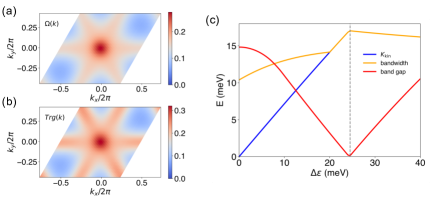
Figure S2: (a) Berry curvature $\Omega(\mathbf{k})$ and (b) trace of quantum metric $\mathrm{Tr}g(\mathbf{k})$ for spin-$\uparrow$ with zero displacement field ($\Delta\varepsilon=0$). (c) Maximum energy difference $K_{\rm kin}=\max(|\varepsilon_{\bm{k},\downarrow}-\varepsilon_{\bm{k},\uparrow}|)$, bandwidth of the top band, and band gap between the first and second highest bands versus the displacement potential $\Delta\varepsilon$. The gray dashed line marks the topological phase transition point.

Figs. S2 (a) and (b) display the Berry curvature $\Omega(\mathbf{k})$ and the trace of the quantum metric $\mathrm{Tr}g(\mathbf{k})$, respectively, for the case of zero displacement field. In Fig. S2 (c), we track how the system evolves with increasing displacement potential: the maximum energy difference between spin bands, $K_{\rm kin}=\max(|\varepsilon_{\bm{k},\downarrow}-\varepsilon_{\bm{k},\uparrow}|)$, the bandwidth of the top band, and the energy gap separating the first and second highest bands are shown as a function of $\Delta\varepsilon$. The topological phase transition is marked by vertical gray dashed line with $\Delta\varepsilon_{c}=24.5~{\rm meV}$.

References

- Xiao et al. [2010] D. Xiao, M.-C. Chang, and Q. Niu, Berry phase effects on electronic properties, Reviews of modern physics 82, 1959 (2010).
- Törmä [2023] P. Törmä, Essay: Where can quantum geometry lead us?, Physical Review Letters 131, 240001 (2023).
- Yu et al. [2024] J. Yu, B. A. Bernevig, R. Queiroz, E. Rossi, P. Törmä, and B.-J. Yang, Quantum geometry in quantum materials, arXiv preprint arXiv:2501.00098 (2024).
- Liu et al. [2025] T. Liu, X.-B. Qiang, H.-Z. Lu, and X. Xie, Quantum geometry in condensed matter, National Science Review 12, nwae334 (2025).
- Marzari et al. [2012] N. Marzari, A. A. Mostofi, J. R. Yates, I. Souza, and D. Vanderbilt, Maximally localized wannier functions: Theory and applications, Reviews of Modern Physics 84, 1419 (2012).
- Törmä et al. [2022] P. Törmä, S. Peotta, and B. A. Bernevig, Superconductivity, superfluidity and quantum geometry in twisted multilayer systems, Nature Reviews Physics 4, 528 (2022).
- Peotta and Törmä [2015] S. Peotta and P. Törmä, Superfluidity in topologically nontrivial flat bands, Nature communications 6, 8944 (2015).
- Xie et al. [2020] F. Xie, Z. Song, B. Lian, and B. A. Bernevig, Topology-bounded superfluid weight in twisted bilayer graphene, Physical review letters 124, 167002 (2020).
- Herzog-Arbeitman et al. [2022] J. Herzog-Arbeitman, V. Peri, F. Schindler, S. D. Huber, and B. A. Bernevig, Superfluid weight bounds from symmetry and quantum geometry in flat bands, Physical review letters 128, 087002 (2022).
- Kwon and Yang [2024] S. Kwon and B.-J. Yang, Quantum geometric bound and ideal condition for euler band topology, Physical Review B 109, L161111 (2024).
- Onishi and Fu [2024a] Y. Onishi and L. Fu, Fundamental bound on topological gap, Physical Review X 14, 011052 (2024a).
- Komissarov et al. [2024] I. Komissarov, T. Holder, and R. Queiroz, The quantum geometric origin of capacitance in insulators, Nature communications 15, 4621 (2024).
- Verma and Queiroz [2024] N. Verma and R. Queiroz, Instantaneous response and quantum geometry of insulators, arXiv preprint arXiv:2403.07052 (2024).
- Onishi and Fu [2024b] Y. Onishi and L. Fu, Topological bound on the structure factor, Physical Review Letters 133, 206602 (2024b).
- Esin et al. [2025] I. Esin, É. Lantagne-Hurtubise, F. Nathan, and G. Refael, Quantum geometry and bounds on dissipation in slowly driven quantum systems, Physical Review Letters 134, 146603 (2025).
- Froese et al. [2025] P. Froese, M. R. Hirsbrunner, and Y. B. Kim, Probing quantum geometry with two-dimensional nonlinear optical spectroscopy (2025), arXiv:2506.05462 [cond-mat.mes-hall] .
- Kattan et al. [2025] J. G. Kattan, A. H. Duff, and J. E. Sipe, Linear response of a chern insulator to finite-frequency electric fields (2025), arXiv:2409.14601 [cond-mat.mes-hall] .
- Zeng and Millis [2025] Y. Zeng and A. J. Millis, Superfluid stiffness bounds in time-reversal symmetric superconductors, arXiv preprint arXiv:2506.18081 (2025).
- von Baltz and Kraut [1981] R. von Baltz and W. Kraut, Theory of the bulk photovoltaic effect in pure crystals, Physical Review B 23, 5590 (1981).
- Sturman and Fridkin [1992] B. I. Sturman and V. M. Fridkin, Photovoltaic and photo-refractive effects in noncentrosymmetric materials, Routledge 10.1201/9780203743416 (1992).
- Hughes and Sipe [1996] J. L. Hughes and J. Sipe, Calculation of second-order optical response in semiconductors, Physical Review B 53, 10751 (1996).
- Sipe and Shkrebtii [2000] J. Sipe and A. Shkrebtii, Second-order optical response in semiconductors, Physical Review B 61, 5337 (2000).
- Pesin [2018] D. Pesin, Two-particle collisional coordinate shifts and hydrodynamic anomalous hall effect in systems without lorentz invariance, Physical Review Letters 121, 226601 (2018).
- Cao et al. [2021] J. Cao, H. A. Fertig, and L. Brey, Quantum geometric exciton drift velocity, Physical Review B 103, 10.1103/physrevb.103.115422 (2021).
- Paiva et al. [2024] C. Paiva, T. Holder, and R. Ilan, Shift and polarization of excitons from quantum geometry, arXiv preprint arXiv:2408.10300 (2024).
- Fertig and Brey [2025] H. Fertig and L. Brey, Many-body quantum geometric dipole, Physical Review B 111, 035158 (2025).
- Estienne et al. [2023] B. Estienne, N. Regnault, and V. Crépel, Ideal chern bands as landau levels in curved space, Physical Review Research 5, L032048 (2023).
- Roy [2014] R. Roy, Band geometry of fractional topological insulators, Physical Review B 90, 165139 (2014).
- Parameswaran et al. [2013] S. A. Parameswaran, R. Roy, and S. L. Sondhi, Fractional quantum hall physics in topological flat bands, Comptes Rendus Physique 14, 816 (2013).
- Crépel et al. [2023] V. Crépel, A. Dunbrack, D. Guerci, J. Bonini, and J. Cano, Chiral model of twisted bilayer graphene realized in a monolayer, Physical Review B 108, 075126 (2023).
- Wang et al. [2021] J. Wang, J. Cano, A. J. Millis, Z. Liu, and B. Yang, Exact landau level description of geometry and interaction in a flatband, Physical review letters 127, 246403 (2021).
- Crépel et al. [2024] V. Crépel, N. Regnault, and R. Queiroz, Chiral limit and origin of topological flat bands in twisted transition metal dichalcogenide homobilayers, Communications Physics 7, 146 (2024).
- Claassen et al. [2015] M. Claassen, C. H. Lee, R. Thomale, X.-L. Qi, and T. P. Devereaux, Position-momentum duality and fractional quantum hall effect in chern insulators, Physical review letters 114, 236802 (2015).
- Crépel et al. [2025] V. Crépel, P. Ding, N. Verma, N. Regnault, and R. Queiroz, Topologically protected flatness in chiral moiré heterostructures, Physical Review X 15, 021056 (2025).
- Shi et al. [2025] J. Shi, J. Cano, and N. Morales-Durán, Effects of berry curvature on ideal band magnetorotons, arXiv preprint arXiv:2503.15900 (2025).
- Marzari and Vanderbilt [1997] N. Marzari and D. Vanderbilt, Maximally localized generalized wannier functions for composite energy bands, Physical review B 56, 12847 (1997).
- Li et al. [2024] Q. Li, J. Dong, P. J. Ledwith, and E. Khalaf, Constraints on real space representations of chern bands, arXiv preprint arXiv:2407.02561 (2024).
- Zhou et al. [2021] H. Zhou, T. Xie, A. Ghazaryan, T. Holder, J. R. Ehrets, E. M. Spanton, T. Taniguchi, K. Watanabe, E. Berg, M. Serbyn, et al., Half-and quarter-metals in rhombohedral trilayer graphene, Nature 598, 429 (2021).
- Zhou et al. [2022] H. Zhou, L. Holleis, Y. Saito, L. Cohen, W. Huynh, C. L. Patterson, F. Yang, T. Taniguchi, K. Watanabe, and A. F. Young, Isospin magnetism and spin-polarized superconductivity in bernal bilayer graphene, Science 375, 774 (2022).
- de la Barrera et al. [2022] S. C. de la Barrera, S. Aronson, Z. Zheng, K. Watanabe, T. Taniguchi, Q. Ma, P. Jarillo-Herrero, and R. Ashoori, Cascade of isospin phase transitions in bernal-stacked bilayer graphene at zero magnetic field, Nature Physics 18, 771 (2022).
- Anderson et al. [2023] E. Anderson, F.-R. Fan, J. Cai, W. Holtzmann, T. Taniguchi, K. Watanabe, D. Xiao, W. Yao, and X. Xu, Programming correlated magnetic states with gate-controlled moiré geometry, Science 381, 325 (2023).
- Cai et al. [2023] J. Cai, E. Anderson, C. Wang, X. Zhang, X. Liu, W. Holtzmann, Y. Zhang, F. Fan, T. Taniguchi, K. Watanabe, et al., Signatures of fractional quantum anomalous hall states in twisted mote2, Nature 622, 63 (2023).
- Park et al. [2023] H. Park, J. Cai, E. Anderson, Y. Zhang, J. Zhu, X. Liu, C. Wang, W. Holtzmann, C. Hu, Z. Liu, T. Taniguchi, K. Watanabe, J.-H. Chu, T. Cao, L. Fu, W. Yao, C.-Z. Chang, D. Cobden, D. Xiao, and X. Xu, Observation of fractionally quantized anomalous Hall effect, Nature 622, 74 (2023).
- Xu et al. [2023] F. Xu, Z. Sun, T. Jia, C. Liu, C. Xu, C. Li, Y. Gu, K. Watanabe, T. Taniguchi, B. Tong, J. Jia, Z. Shi, S. Jiang, Y. Zhang, X. Liu, and T. Li, Observation of integer and fractional quantum anomalous hall effects in twisted bilayer , Phys. Rev. X 13, 031037 (2023).
- Zeng et al. [2023] Y. Zeng, Z. Xia, K. Kang, J. Zhu, P. Knüppel, C. Vaswani, K. Watanabe, T. Taniguchi, K. F. Mak, and J. Shan, Thermodynamic evidence of fractional chern insulator in moirémote2, Nature 622, 69 (2023).
- Han et al. [2023] T. Han, Z. Lu, G. Scuri, J. Sung, J. Wang, T. Han, K. Watanabe, T. Taniguchi, L. Fu, H. Park, et al., Orbital multiferroicity in pentalayer rhombohedral graphene, Nature 623, 41 (2023).
- Lu et al. [2024] Z. Lu, T. Han, Y. Yao, A. P. Reddy, J. Yang, J. Seo, K. Watanabe, T. Taniguchi, L. Fu, and L. Ju, Fractional quantum anomalous hall effect in multilayer graphene, Nature 626, 759 (2024).
- Han et al. [2024] T. Han, Z. Lu, G. Scuri, J. Sung, J. Wang, T. Han, K. Watanabe, T. Taniguchi, H. Park, and L. Ju, Correlated insulator and chern insulators in pentalayer rhombohedral-stacked graphene, Nature Nanotechnology 19, 181 (2024).
- Foutty et al. [2024] B. A. Foutty, C. R. Kometter, T. Devakul, A. P. Reddy, K. Watanabe, T. Taniguchi, L. Fu, and B. E. Feldman, Mapping twist-tuned multiband topology in bilayer wse2, Science 384, 343 (2024).
- Gao et al. [2025] B. Gao, M. Ghafariasl, M. J. Mehrabad, T.-S. Huang, L. Zhang, D. Session, P. Upadhyay, R. Ma, G. Alshalan, D. G. S. Forero, et al., Probing quantum anomalous hall states in twisted bilayer wse2 via attractive polaron spectroscopy, arXiv preprint arXiv:2504.11530 (2025).
- Xie et al. [2025a] J. Xie, Z. Huo, X. Lu, Z. Feng, Z. Zhang, W. Wang, Q. Yang, K. Watanabe, T. Taniguchi, K. Liu, Z. Song, X. C. Xie, J. Liu, and X. Lu, Tunable fractional chern insulators in rhombohedral graphene superlattices, Nature Materials 10.1038/s41563-025-02225-7 (2025a).
- Kennes et al. [2021] D. M. Kennes, M. Claassen, L. Xian, A. Georges, A. J. Millis, J. Hone, C. R. Dean, D. Basov, A. N. Pasupathy, and A. Rubio, Moiré heterostructures as a condensed-matter quantum simulator, Nature Physics 17, 155 (2021).
- Nuckolls and Yazdani [2024] K. P. Nuckolls and A. Yazdani, A microscopic perspective on moiré materials, Nature Reviews Materials 9, 460 (2024).
- Crépel and Millis [2024a] V. Crépel and A. Millis, Bridging the small and large in twisted transition metal dichalcogenide homobilayers: A tight binding model capturing orbital interference and topology across a wide range of twist angles, Physical Review Research 6, 033127 (2024a).
- Shi et al. [2019] L.-k. Shi, J. Ma, and J. C. Song, Gate-tunable flat bands in van der waals patterned dielectric superlattices, 2D Materials 7, 015028 (2019).
- Ghorashi et al. [2023] S. A. A. Ghorashi, A. Dunbrack, A. Abouelkomsan, J. Sun, X. Du, and J. Cano, Topological and stacked flat bands in bilayer graphene with a superlattice potential, Physical Review Letters 130, 196201 (2023).
- Ghorashi and Cano [2023] S. A. A. Ghorashi and J. Cano, Multilayer graphene with a superlattice potential, Physical Review B 107, 195423 (2023).
- Krix and Sushkov [2023] Z. Krix and O. P. Sushkov, Patterned bilayer graphene as a tunable strongly correlated system, Physical Review B 107, 165158 (2023).
- Gao et al. [2023] Q. Gao, J. Dong, P. Ledwith, D. Parker, and E. Khalaf, Untwisting moiré physics: Almost ideal bands and fractional chern insulators in periodically strained monolayer graphene, Phys. Rev. Lett. 131, 096401 (2023).
- Wan et al. [2023] X. Wan, S. Sarkar, S.-Z. Lin, and K. Sun, Topological exact flat bands in two-dimensional materials under periodic strain, Physical Review Letters 130, 216401 (2023).
- Zeng et al. [2024a] Y. Zeng, T. M. Wolf, C. Huang, N. Wei, S. A. A. Ghorashi, A. H. MacDonald, and J. Cano, Gate-tunable topological phases in superlattice modulated bilayer graphene, Physical Review B 109, 195406 (2024a).
- Seleznev et al. [2024] D. Seleznev, J. Cano, and D. Vanderbilt, Inducing topological flat bands in bilayer graphene with electric and magnetic superlattices, Physical Review B 110, 205115 (2024).
- Sun et al. [2024] J. Sun, S. A. Akbar Ghorashi, K. Watanabe, T. Taniguchi, F. Camino, J. Cano, and X. Du, Signature of correlated insulator in electric field controlled superlattice, Nano Letters 24, 13600 (2024).
- Ault-McCoy et al. [2025] D. Ault-McCoy, M. N. Y. Lhachemi, A. Dunbrack, S. A. A. Ghorashi, and J. Cano, Optimizing superlattice bilayer graphene for a fractional chern insulator, arXiv preprint arXiv:2505.05551 (2025).
- Regnault and Bernevig [2011] N. Regnault and B. A. Bernevig, Fractional chern insulator, Physical Review X 1, 021014 (2011).
- Neupert et al. [2011] T. Neupert, L. Santos, C. Chamon, and C. Mudry, Fractional quantum hall states at zero magnetic field, Physical Review Letters 106, 10.1103/physrevlett.106.236804 (2011).
- Sheng et al. [2011] D. Sheng, Z.-C. Gu, K. Sun, and L. Sheng, Fractional quantum hall effect in the absence of landau levels, Nature Communications 2, 10.1038/ncomms1380 (2011).
- Crépel and Millis [2024b] V. Crépel and A. Millis, Spinon pairing induced by chiral in-plane exchange and the stabilization of odd-spin chern number spin liquid in twisted mote 2, Physical Review Letters 133, 146503 (2024b).
- Levin and Stern [2009] M. Levin and A. Stern, Fractional topological insulators, Physical Review Letters 103, 10.1103/physrevlett.103.196803 (2009).
- Crépel and Regnault [2024] V. Crépel and N. Regnault, Attractive haldane bilayers for trapping non-abelian anyons, Physical Review B 110, 115109 (2024).
- Xie et al. [2025b] F. Xie, L. Chen, S. Sur, Y. Fang, J. Cano, and Q. Si, Superconductivity in twisted wse 2 from topology-induced quantum fluctuations, Physical Review Letters 134, 136503 (2025b).
- Stern [2016] A. Stern, Fractional topological insulators: A pedagogical review, Annual Review of Condensed Matter Physics 7, 349–368 (2016).
- Crépel and Fu [2023] V. Crépel and L. Fu, Anomalous hall metal and fractional chern insulator in twisted transition metal dichalcogenides, Physical Review B 107, L201109 (2023).
- Morales-Durán et al. [2023] N. Morales-Durán, J. Wang, G. R. Schleder, M. Angeli, Z. Zhu, E. Kaxiras, C. Repellin, and J. Cano, Pressure-enhanced fractional chern insulators along a magic line in moiré transition metal dichalcogenides, Phys. Rev. Res. 5, L032022 (2023).
- Repellin et al. [2020] C. Repellin, Z. Dong, Y.-H. Zhang, and T. Senthil, Ferromagnetism in narrow bands of moiré superlattices, Physical Review Letters 124, 187601 (2020).
- Muñoz-Segovia et al. [2025] D. Muñoz-Segovia, V. Crépel, R. Queiroz, and A. J. Millis, Twist-angle evolution of the intervalley-coherent antiferromagnet in twisted wse , arXiv preprint arXiv:2503.11763 (2025).
- Young and Rappe [2012] S. M. Young and A. M. Rappe, First principles calculation of the shift current photovoltaic effect in ferroelectrics, Physical review letters 109, 116601 (2012).
- Morimoto and Nagaosa [2016] T. Morimoto and N. Nagaosa, Topological aspects of nonlinear excitonic processes in noncentrosymmetric crystals, Physical Review B 94, 035117 (2016).
- Fei et al. [2020] R. Fei, L. Z. Tan, and A. M. Rappe, Shift-current bulk photovoltaic effect influenced by quasiparticle and exciton, Physical Review B 101, 045104 (2020).
- Kaplan et al. [2022] D. Kaplan, T. Holder, and B. Yan, Twisted photovoltaics at terahertz frequencies from momentum shift current, Physical Review Research 4, 013209 (2022).
- Chaudhary et al. [2022] S. Chaudhary, C. Lewandowski, and G. Refael, Shift-current response as a probe of quantum geometry and electron-electron interactions in twisted bilayer graphene, Physical Review Research 4, 013164 (2022).
- Lee et al. [2023] H. Lee, Y. B. Kim, J. W. Ryu, S. Kim, J. Bae, Y. Koo, D. Jang, and K.-D. Park, Recent progress of exciton transport in two-dimensional semiconductors, Nano Convergence 10, 57 (2023).
- Nakamura et al. [2024] M. Nakamura, Y.-H. Chan, T. Yasunami, Y.-S. Huang, G.-Y. Guo, Y. Hu, N. Ogawa, Y. Chiew, X. Yu, T. Morimoto, et al., Strongly enhanced shift current at exciton resonances in a noncentrosymmetric wide-gap semiconductor, Nature Communications 15, 9672 (2024).
- Haber et al. [2023] J. B. Haber, D. Y. Qiu, F. H. da Jornada, and J. B. Neaton, Maximally localized exciton wannier functions for solids, Phys. Rev. B 108, 125118 (2023).
- Fukui et al. [2005] T. Fukui, Y. Hatsugai, and H. Suzuki, Chern numbers in discretized brillouin zone: efficient method of computing (spin) hall conductances, Journal of the Physical Society of Japan 74, 1674 (2005).
- Fukui and Hatsugai [2007] T. Fukui and Y. Hatsugai, Topological aspects of the quantum spin-hall effect in graphene: Z 2 topological order and spin chern number, Physical Review B—Condensed Matter and Materials Physics 75, 121403 (2007).
- Note [1] Gauge invariance of the quantum-geometric dipole is straightforwardly checked by substituting in Eq. 2.
- Berry [1984] M. V. Berry, Quantal phase factors accompanying adiabatic changes, Proceedings of the Royal Society of London. A. Mathematical and Physical Sciences 392, 45 (1984).
- Wu and Sarma [2020] F. Wu and S. D. Sarma, Quantum geometry and stability of moiré flatband ferromagnetism, Physical Review B 102, 165118 (2020).
- Crépel et al. [2021] V. Crépel, A. Hackenbroich, N. Regnault, and B. Estienne, Universal signatures of dirac fermions in entanglement and charge fluctuations, Physical Review B 103, 235108 (2021).
- Crépel et al. [2020] V. Crépel, B. Estienne, and N. Regnault, Microscopic study of the coupled-wire construction and plausible realization in spin-dependent optical lattices, Physical Review B 101, 235158 (2020).
- Abouelkomsan et al. [2023] A. Abouelkomsan, K. Yang, and E. J. Bergholtz, Quantum metric induced phases in moiré materials, Physical Review Research 5, L012015 (2023).
- Zeng et al. [2024b] Y. Zeng, D. Guerci, V. Crépel, A. J. Millis, and J. Cano, Sublattice structure and topology in spontaneously crystallized electronic states, Physical Review Letters 132, 236601 (2024b).
- Fang et al. [2024] Y. Fang, J. Cano, and S. A. A. Ghorashi, Quantum geometry induced nonlinear transport in altermagnets, Physical Review Letters 133, 106701 (2024).
- Crépel and Cano [2025] V. Crépel and J. Cano, Efficient prediction of superlattice and anomalous miniband topology from quantum geometry, Physical Review X 15, 011004 (2025).
- Nambu [1960] Y. Nambu, Quasi-particles and gauge invariance in the theory of superconductivity, Physical Review 117, 648 (1960).
- Goldstone [1961] J. Goldstone, Field theories with superconductor solutions, Il Nuovo Cimento (1955-1965) 19, 154 (1961).
- Nielsen and Chadha [1976] H. B. Nielsen and S. Chadha, On how to count goldstone bosons, Nuclear Physics B 105, 445 (1976).
- Watanabe and Murayama [2012] H. Watanabe and H. Murayama, Unified description of nambu-goldstone bosons without lorentz invariance, Physical Review Letters 108, 251602 (2012).
- Bernevig et al. [2006] B. A. Bernevig, T. L. Hughes, and S.-C. Zhang, Quantum spin hall effect and topological phase transition in hgte quantum wells, science 314, 1757 (2006).
- Wu et al. [2019] F. Wu, T. Lovorn, E. Tutuc, I. Martin, and A. MacDonald, Topological insulators in twisted transition metal dichalcogenide homobilayers, Physical review letters 122, 086402 (2019).
- Devakul et al. [2021] T. Devakul, V. Crépel, Y. Zhang, and L. Fu, Magic in twisted transition metal dichalcogenide bilayers, Nature communications 12, 6730 (2021).
- Wang et al. [2024] C. Wang, X.-W. Zhang, X. Liu, Y. He, X. Xu, Y. Ran, T. Cao, and D. Xiao, Fractional chern insulator in twisted bilayer , Phys. Rev. Lett. 132, 036501 (2024).
- Jia et al. [2024] Y. Jia, J. Yu, J. Liu, J. Herzog-Arbeitman, Z. Qi, H. Pi, N. Regnault, H. Weng, B. A. Bernevig, and Q. Wu, Moiré fractional chern insulators. i. first-principles calculations and continuum models of twisted bilayer , Phys. Rev. B 109, 205121 (2024).