Spin Seebeck Effect of Triangular-lattice Spin Supersolid

Abstract

Using our developed thermal tensor-network approach, we investigate the spin Seebeck effect (SSE) of the triangular-lattice quantum antiferromagnet hosting spin supersolid phase. We focus on the low-temperature scaling of normalized spin current $\tilde{I}_{S}$ through the interface, and benchmark our approach on 1D Heisenberg chain, with the negative spinon spin current reproduced. In addition, we find an algebraic scaling $\tilde{I}_{S}\sim T^{\alpha}$ with varying exponent $\alpha$ in the Tomonaga-Luttinger liquid phase. On the triangular lattice, spin frustration dramatically enhances the low-temperature SSE, with characteristic spin-current signatures distinguishing different magnetic phases. Remarkably, we discover a persistent spin current $\tilde{I}_{S}$ in the spin supersolid phase, which saturates to a non-zero value in the low-temperature limit and can be ascribed to the Goldstone-mode-mediated spin supercurrents. Moreover, a universal scaling $\tilde{I}_{S}\sim T^{d/z}$ is found at the U(1)-symmetric polarization quantum critical points. These distinct quantum spin transport traits — particularly the sign reversal and characteristic temperature dependence in SSE — provide sensitive experimental probes for investigating spin-supersolid compounds such as Na₂BaCo(PO₄)₂. Moreover, our results establish spin supersolids as a tunable quantum platform for spin caloritronics in the ultralow-temperature regime.

Introduction.— Quantum magnets represent fascinating correlated materials that host a rich variety of exotic phases and emergent phenomena. In one-dimensional (1D) systems, spin Tomonaga-Luttinger liquid (TLL) with spinon excitations emerges [1, 2, 3], while higher-dimensional frustrated lattices possess even richer phases — including spin liquids [4, 5, 6, 7, 8] and spin supersolids [9, 10, 11, 12, 13, 14], etc. Recently, triangular-lattice quantum antiferromagnets Na₂BaCo(PO₄)₂ [15, 16, 17, 18, 19, 20, 21, 22, 23, 24, 25, 26, 27, 13, 14, 28, 29] and K₂Co(SeO₃)₂ [30, 31, 32, 33, 34, 35] have been proposed to realize spin supersolid phases. The discovery of quantum spin supersolids has opened new avenues for exploring its entropic effect for extreme magnetic cooling [14]. As revealed in neutron scattering measurements [32, 31, 28, 25] and also dynamical simulations [28, 34, 36], the spin supersolid can host rich magnetic excitations including Goldstone modes, roton-like dispersion, and excitation continua.

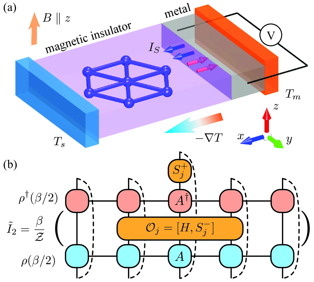
Figure 1: (a) Schematic SSE setup: the (triangular-lattice) quantum magnet (with temperature $T_{s}$) and metal substrate ($T_{m}$) maintain a temperature difference $\delta T=T_{s}-T_{m}$. The resulting spin current $I_{S}$ flows across the magnet-metal interface along the $x$-axis, parallel to the thermal gradient $-\nabla T$. Red(blue) arrow represents the direction of the positive(negative) current. A perpendicular magnetic field $B$ is applied along the $z$-axis, and the spin current is measured by the voltage $V$ along the $y$-axis through the inverse spin Hall effect in the metal substrate. (b) The spin current $\tilde{I}_{2}$ is efficiently computed by contracting the density matrix operator $\rho(\beta/2)$ with its Hermitian conjugate (represented by matrix product of tensors $A$ and $A^{\dagger}$), while incorporating the inserted operators $\mathcal{O}_{j}$ and $S_{j}^{+}$.

An intriguing question thus emerges: Do these spin excitations generate novel transport phenomena in spin supersolids? In particular, the hallmark quantum transport signature — dissipationless spin superflow — has yet to be demonstrated. Thermal conductivity measurements have been conducted on Na₂BaCo(PO₄)₂ (NBCP), which have produced contradictory reports of residual conductivity [16, 19], possibly due to the complex interplay between phonon dynamics, disorder effects, and spin-phonon couplings [37, 38, 39]. On the other hand, the spin Seebeck effect (SSE), as a spin-selective transport probe [40, 41, 42, 43], can offer direct access to spin current yet remains underexplored in quantum magnets, particularly spin supersolids. The SSE is a spin analog of the Seebeck effect in magnetic compounds [44, 45], and reflects spin excitations by generating spin currents from thermal gradients [46, 47, 48, 49, 50, 51]. Recently, there have been theoretical studies on the sign of spin currents in spin chains [50, 52] and Kitaev magnets [53], based on the ground-state calculations. However, fundamental gaps remain in understanding their temperature dependence — especially the scaling behaviors near quantum critical points (QCPs) and in strongly correlated regimes. It arises from the inherent difficulties in simulating the SSE at finite temperature, where quantum and thermal fluctuations exhibit intriguing interplay.

In this work, we develop an efficient thermal tensor-network approach to compute the normalized spin currents ($\tilde{I}_{S}$) and their temperature scaling within an imaginary-time framework. We benchmark the approach on 1D Heisenberg chain with spin TLL phase, and identify the negative spinon spin current $\tilde{I}_{S}\sim-T^{\alpha}$ with an exponent $\alpha$. We then apply the approach to the triangular-lattice spin-supersolid system, and demonstrate how spin currents probe the distinct quantum spin states and map the phase diagram through their temperature dependence. Particularly, we discover a persistent spin current that saturate to a constant in the zero-temperature limit. Momentum-resolved analysis demonstrates that such spin currents are mediated by dissipationless Goldstone modes — a signature of spin supercurrent [54, 55, 56]. Across 1D and 2D Heisenberg systems, we uncover a universal scaling $\tilde{I}_{S}\sim T^{d/z}$ near U(1)-symmetric polarization QCP. Our predicted SSE features can be experimentally investigated on spin-supersolid compounds Na₂BaCo(PO₄)₂ [13, 14] and also K₂Co(SeO₃)₂ [32, 31].

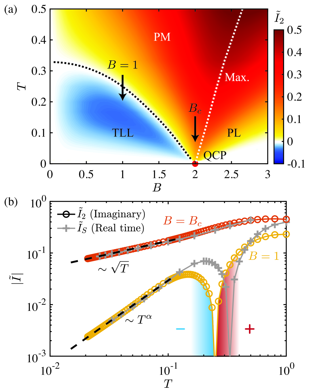
Figure 2: Benchmarks on normalized spin current in 1D Heisenberg chain ($L=128$, $D=500$). (a) The simulated spin current $\tilde{I}_{2}$, where the black dotted line marks the sign reversal, and the white dotted line locates the maximum of $\tilde{I}_{2}$ under a fixed field. The red dot labels the QCP at $B_{c}=2$, separating the TLL and polarized (PL) phases. (b) presents the temperature dependence of spin currents calculated through real-time dynamics ($\tilde{I}_{S}$, with $t_{\rm max}=40$ and $D=500$) and imaginary-time correlations ($\tilde{I}_{2}$). In the TLL phase with $B=1$, an algebraic-decay spin current $\tilde{I}_{S,2}\sim T^{\alpha}$ emerges with $\alpha\simeq 1.59(2)$. At the QCP $B=B_{c}$, a universal scaling $\tilde{I}_{S,2}\sim\sqrt{T}$ is revealed. Due to the undetermined prefactor in the simulated spin currents, we shift the $\tilde{I}_{S}$ data to align with the low-temperature $\tilde{I}_{2}$.

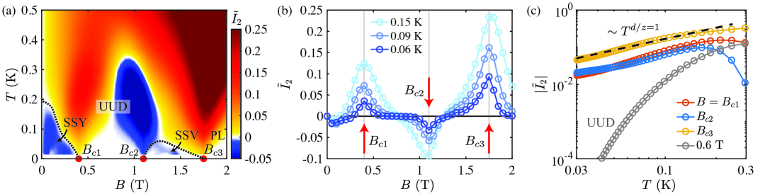
Figure 3: (a) Simulated spin current $\tilde{I}_{2}$ of TLAF model (6$\times$18 cylinder, $D=3000$) for NBCP [13]. Three QCPs $B_{c1,2,3}$ (red dots) separate supersolid-Y (SSY), up-up-down (UUD), supersolid-V (SSV), and the PL phases. Dashed lines indicate schematic phase boundaries of SSY and SSV determined from the sign reversal in $\tilde{I}_{2}$. (b) Isothermal $\tilde{I}_{2}$ cuts reveal three QCPs at $B_{c1}\simeq 0.4$ T, $B_{c2}\simeq 1.1$ T, and $B_{c3}\simeq 1.75$ T (vertical gray lines), where $\tilde{I}_{2}$ exhibits prominent peaks or dips. (c) $\tilde{I}_{2}\sim T^{d/z}$ with $d/z=1$ (black dashed line) at QCPs ($B_{c1,2,3}$). The exponentially decaying $\tilde{I}_{2}$ within the UUD phase ($B=0.6~{\rm T}$) is also plotted as a comparison.

Thermal tensor-network calculations of spin current.— Here we consider the XXZ Heisenberg model under a magnetic field, i.e.,

$$H=\sum_{\langle i,j\rangle}\frac{J_{xy}}{2}(S_{i}^{+}S_{j}^{-}+S_{i}^{-}S_{j}^{+})+J_{z}S_{i}^{z}S_{j}^{z}-B\sum_{i}S_{i}^{z}$$ (1)

with $J_{xy},J_{z}>0$ the nearest-neighboring antiferromagnetic exchange couplings, and $B$ is the external field. As shown in Fig. 1(a), the spin current $I_{S}$ across the magnet-metal interface is driven by temperature gradient and expressed as $I_{S}=-A\tilde{I}_{S}\delta T$, where $A$ denotes a material-dependent constant and $\delta T\equiv T_{s}-T_{m}$ represents the temperature difference between the metal and insulator. Derived through non-equilibrium Green’s function formalism [48, 43, 57], the normalized spin current $\tilde{I}_{S}$ takes the form

$$\tilde{I}_{S}=\int_{-\infty}^{\infty}~d\omega~k^{2}(\beta\omega)\,\mathrm{Im}[\chi^{-+}_{\mathrm{loc}}(\omega)],$$ (2)

with kernel function $k(x)=x/\sinh(x/2)$, where $x\equiv\beta\omega$ and $\beta\equiv 1/T$ [58]. The local dynamical susceptibility $\chi^{-+}_{\mathrm{loc}}(\omega)$ is the central quantity of interest for determining the spin current. One approach for $\tilde{I}_{S}$ involves computing $\mathrm{Im}[\chi^{-+}_{\mathrm{loc}}(\omega)]$ in the ground state [53, 52], while incorporating temperature influences solely through the kernel function $k^{2}(\beta\omega)$. This strategy circumvents the need for calculating $\mathrm{Im}[\chi^{-+}_{\mathrm{loc}}(\omega)]$ at finite temperature, significantly reducing computational cost while trading off precise temperature dependence. Moreover, even with such simplification, there is rapid entanglement growth in the real-time evolution for 2D systems like the triangular-lattice spin supersolid, presenting great computational challenges.

To accurately account for the temperature dependence of ${\rm Im}[\chi^{-+}_{\mathrm{loc}}(\omega)]$ while avoiding real-time evolution, we develop an alternative, thermal tensor-network method based on the imaginary-time framework. Given the analyticity of ${\rm Im}[\chi^{-+}_{\rm loc}(\omega)]$ near $\omega=0$, we perform the expansion ${\rm Im}[\chi^{-+}_{\rm loc}(\omega)]=\sum_{n=1}^{\infty}\frac{\omega^{n}}{n!}f_{n}$. The even parity of the kernel function $k(\beta\omega)$ selects $f_{2}$ as the leading term, resulting in the dominant contribution $\tilde{I}_{S}\sim f_{2}/\beta^{3}$, which accurately captures the low-temperature scaling for $\beta\omega\lesssim{O}(1)$ [58]. On the other hand, we examine the local imaginary-time correlation function and find $\frac{\partial}{\partial\tau}\langle S^{-}_{j}(\tau)S^{+}_{j}\rangle\Big{|}_{\tau=\beta/2}=\frac{1}{2\beta\pi}\int_{-\infty}^{\infty}d\omega\,k(\beta\omega)\,{\rm Im}[\chi_{\rm loc}^{-+}(\omega)]=\frac{f_{2}}{\beta^{4}}+O(\frac{1}{\beta^{6}})\sim\frac{\tilde{I}_{S}}{\beta}$, where ${\rm Im}[\chi_{\text{loc}}^{-+}(\omega)]$ is also expanded up to second order. Therefore, the spin current in the low-temperature regime can be calculated as

$$\tilde{I}_{2}=\beta\langle\mathcal{O}_{j}(\frac{\beta}{2})S_{j}^{+}\rangle_{\beta}.$$ (3)

Here $\mathcal{O}_{j}=[H_{,}S_{j}^{-}]$ is a local operator satisfying $\frac{\partial}{\partial\tau}\langle S^{-}_{j}(\tau)S^{+}_{j}\rangle\Big{|}_{\tau=\beta/2}=\langle\mathcal{O}_{j}(\beta/2)S_{j}^{+}\rangle_{\beta}$, and Eq. (3) is dubbed as the imaginary-time approximation (ITA). In practice, using the tangent-space tensor renormalization group (tanTRG) method [59], we prepare the thermal density matrix $\rho(\beta/2)=e^{-\beta H/2}$ in the matrix product operator form. Subsequently, the imaginary-time correlation function and thus $\tilde{I}_{2}$ can be obtained through the tensor-network contraction scheme depicted in Fig. 1(b).

Benchmarks on 1D Heisenberg spin chain.— We begin by analyzing the isotropic Heisenberg spin chain ($J_{xy}=J_{z}=1$), where spin currents are computed using our thermal tensor network method for a finite-size system (see Appendix for technical details). In Figure 2(a), we show the contour plot of $\tilde{I}_{2}$ from the ITA calculations, which reveals a characteristic sign reversal that locates the crossover between the low-temperature TLL (negative) and the high-temperature paramagnetic regimes (positive). The negative spin current has been observed in spin-chain compounds and attributed to spinon excitations [50]. To validate the ITA approach, we also perform real-time calculations of $\tilde{I}_{S}$ through Eq. (2) as a benchmark [58]. The real-time dynamical correlation function and corresponding local susceptibility ${\rm Im}[\chi_{\text{loc}}^{-+}(\omega)]$ are evaluated using tensor network method that combines finite-temperature tanTRG [59] and time-dependent variational principle approach for real-time dynamics [60, 61, 58].

As shown in Fig. 2(b), we find both $\tilde{I}_{S}$ and $\tilde{I}_{2}$ exhibit consistent temperature scaling at low temperature ($T\lesssim 0.1$) and across distinct regimes, validating the ITA method. In the TLL phase (with $B=1$), the spin current follows $|\tilde{I}_{S,2}|\sim T^{\alpha}$, reflecting the gapless spinon excitation. We note that while the TLL theory with nonlinear spinon dispersion can reproduce the algebraic spinon spin current [50, 52], there are challenges to accurately determine the varying critical exponents $\alpha$ in the TLL phase [58]. At the QCP ($B_{c}=2$), we find a universal scaling $\tilde{I}_{S,2}\sim\sqrt{T}$ in both real- and imaginary-time approaches (see Appendix). This consistency demonstrates ITA as an accurate and efficient approach for SSE simulations.

SSE in a triangular-lattice quantum antiferromagnet.— The easy-axis triangular-lattice antiferromagnet (TLAF) with $J_{z}>J_{xy}$ [Eq. (1)] realizes the long-predicted spin supersolid state [9, 10, 13]. This exotic phase has recently been experimentally observed in Co-based quantum magnets including Na₂BaCo(PO₄)₂ [15, 16, 20, 14] and K₂Co(SeO₃)₂ [30, 32, 31]. In the former compound, an effective model with coupling strength $J_{xy}=0.88~{\rm K}$, $J_{z}=1.48~{\rm K}$ and the Landé factor $g_{z}=4.89$ accurately describes its magnetic [16, 17, 14] and dynamical properties [20, 28, 25]. We hereafter simulate SSE in the TLAF model using NBCP parameters, noting that our results also extend to other spin-supersolid materials like K₂Co(SeO₃)₂ that share the same easy-axis TLAF model.

As observed in experiments [16, 20, 14] and comprehended in theoretical calculations [13], the NBCP exhibits four distinct phases: supersolid-Y (SSY), up-up-down (UUD), supersolid-V (SSV), and polarized (PL) phases. They are separated by three QCPs located at $B_{c1}\simeq 0.35(5)$ T, $B_{c2}\simeq 1.15(4)$ T, and $B_{c3}\simeq 1.69(6)$ T [14]. In both SSY and SSV phases, the system exhibits simultaneous breaking of lattice translation symmetry and U(1) rotation symmetry, establishing a quantum magnetic analog of supersolid [62, 63, 64, 65, 66, 67].

Figure 3(a) reveals the rich characteristic behaviors of spin currents, which can be used to map the finite-temperature phase diagram of NBCP. The different spin-current signs and their thermal evolution distinguish different quantum phases. Both supersolid phases (SSY and SSV) can be recognized by the negative spin currents, where the sign reversal marks the transition from higher-temperature states to the spin-supersolid phase. In contrast, in the UUD phase between $B_{c1}$ and $B_{c2}$, the spin current decays rapidly at low temperature [see Fig. 3(c)] due to its gapped nature; the PL regime shows persistently a positive sign.

Figure 3(b) demonstrates the precise detection of all three QCPs through SSE measurements. The peaks and dips in the spin current profile show excellent agreement with established QCP locations from prior studies [16, 13, 14], again confirming the reliability and accuracy of our ITA approach. Moreover, Fig. 3(c) shows the linear temperature dependence of $\tilde{I}_{2}$ near three QCPs, consistent with quantum critical scaling $\tilde{I}_{2}\sim T^{d/z}$ ($d=2,z=2$). This universal enhancement of spin current originates from the gapless excitations of QCPs, and reflects the low-energy density of states encoded in the symmetric part of the local dynamical susceptibility $\frac{1}{2}{\rm Im}\left[\chi^{-+}_{\rm loc}(\omega)+\chi^{-+}_{\rm loc}(-\omega)\right]\sim\omega^{(d-z)/z}$ (see Appendix). Note the linear temperature scaling of spin current near the saturation QCP, belonging to the Bose-Einstein condensation universality class [68, 69], can be captured by the spin-wave calculations [58].

Spin current sign reversal.— To understand the sign reversal in the spin supersolid phase, we decompose the local operator as $\mathcal{O}_{j}=\mathcal{O}_{j}^{J}+\mathcal{O}_{j}^{B}$, where $\mathcal{O}_{j}^{J}=[H_{0},S_{j}^{-}]=\sum_{\langle i,j\rangle}(J_{xy}S_{i}^{-}S_{j}^{z}-J_{z}S_{i}^{z}S_{j}^{-})$ and $\mathcal{O}_{j}^{B}=[-B\sum_{i}S_{i}^{z},S_{j}^{-}]=BS_{j}^{-}$. We then compute the component $\tilde{I}_{2}^{J}=\beta\langle\mathcal{O}_{j}^{J}(\frac{\beta}{2})S_{j}^{+}\rangle_{\beta}$ stemming from spin exchange and $\tilde{I}_{2}^{B}=\beta\langle\mathcal{O}_{j}^{B}(\frac{\beta}{2})S_{j}^{+}\rangle_{\beta}$ from Zeeman coupling, with the total current $\tilde{I}_{2}=\tilde{I}_{2}^{J}+\tilde{I}_{2}^{B}$. We find that the spin exchange generates a negative spin current ($\tilde{I}^{J}_{2}<0$) while the Zeeman term leads to positive contributions ($\tilde{I}^{B}_{2}>0$, see Appendix). Therefore, the sign reversal in spin supersolid phase can be regarded as a consequence of the competition between exchange coupling and Zeeman-term effects — the interaction plays a dominant role at low temperatures and thus gives rise to a negative spin current. Note such sign reversal in spin supersolid is not captured by linear spin-wave theory (see Appendix). Moreover, in the PL regime ($B\geq B_{c3}$), strong magnetic fields suppress exchange effects, resulting in exclusively positive spin currents across the whole temperature window [see Fig. 3(a)].

Within the UUD phase, we observe a field-driven sign reversal of the spin current — positive at lower fields and negative at higher fields — with the boundary at the magnetization plateau midpoint [Fig. 3(a,b)]. This phenomenon can be explained by examining the temperature dependence of magnetization [58]: At the plateau midpoint where $\frac{dM}{dT}=0$, spin current vanishes when $M$ becomes temperature-independent. Moving away from this point, the sign of spin current follows $(-\frac{dM}{dT})$ — positive when $\frac{dM}{dT}<0$ and negative when $\frac{dM}{dT}>0$. Since $\frac{dM}{dT}$ quantifies the magnetocaloric effect (MCE), such observation reveals inherent connections between SSE and MCE [58].

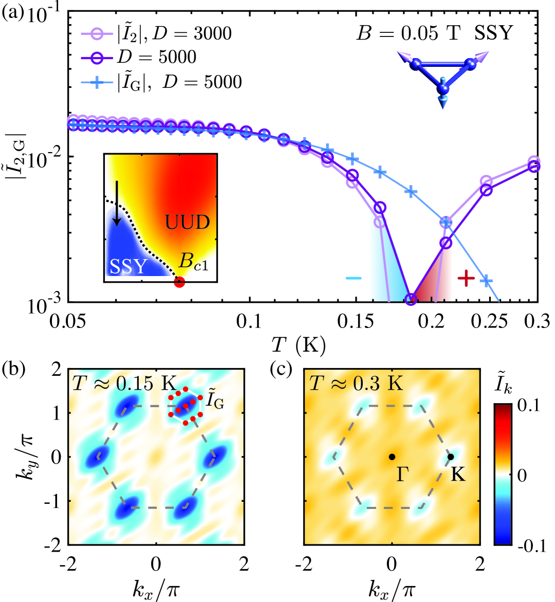
Figure 4: (a) The simulated $\tilde{I}_{2}$ results in the SSY phase under $B=0.05$ T (see inset), where the data are well converged with $D=5000$. (b) and (c) present the momentum-resolved spin current $\tilde{I}_{k}$ at two temperatures. The gray dashed line shows the boundary of the 1st Brillouin zone. The red dots mark the involved momentum points in the calculations of $\tilde{I}_{\rm G}$. The black dots label the $\Gamma$ and the K point respectively.

Spin supercurrent in the supersolid phase.— The nonzero spin superfluid density — unusual in easy-axis systems — characterizes the spin supersolid phase, quantified by spin stiffness [70] and manifesting in distinct transport signatures. Figure 4(a) reveals a striking spin current behavior across the UUD-to-SSY transition: Sign reversal upon entering the SSY phase, and persistent negative current that saturates to a nonzero value at low temperatures, revealing a quantum transport signature of the spin supersolid phase.

To elucidate the origin of negative spin supercurrents, we compute the momentum-resolved current $\tilde{I}_{k}=\beta\langle\mathcal{O}_{-k}(\beta/2)S_{k}^{+}\rangle$ (where $S_{k}^{+}=\frac{1}{\sqrt{N}}\sum_{n}e^{ikn}S_{n}^{+}$ and $\mathcal{O}_{k}=[H,S_{k}^{-}]$), indicating distinct temperature-dependent behaviors in Fig. 4(b,c): At $T=0.3$ K, most momentum points contribute positively to the net current; while at $T=0.15$ K, gapless Goldstone modes near the K point dominate with negative contributions. By isolating these modes through $\tilde{I}_{\rm G}=\frac{2}{N}\sum_{k\in k_{\rm G}}\tilde{I}_{k}$ [with $k_{\rm G}$ marked in Fig. 4(b)], we establish the saturated $\tilde{I}_{\rm G}\approx\tilde{I}_{2}$ at low temperatures [Fig. 4(a)]. The positive angular momentum of K-point Goldstone modes (versus $\Gamma$-point modes) yields $dM/dT>0$ when K-magnon populations increase, producing negative spin currents.

Therefore, we demonstrate how dissipationless Goldstone modes maintain persistent spin supercurrents in the supersolid phase. Unlike the exponential decay in UUD phase [Fig. 3(c)], the easy-axis system sustains persistent currents despite out-of-plane UUD ordering [Fig. 4(a) and inset] — providing quantum transport probe for spin supersolidity with clear experimental signatures in future studies.

Discussion.— We develop a thermal tensor-network approach to investigate SSE in quantum magnets. Our approach enables accurate calculations of spin currents and their temperature dependence, which successfully resolves the negative algebraic spinon current in 1D TLLs. Remarkably, in 2D triangular-lattice spin supersolids, we observe persistent spin supercurrents that saturate at low temperatures — a SSE signature directly linked to dissipationless Goldstone-mode excitations. Furthermore, we uncover universal scaling of the normalized spin Seebeck current ($\tilde{I}_{S}\sim T^{d/z}$) near polarization QCPs, a behavior consistently observed across both 1D and 2D systems. Our work enables the first systematic investigation of spin-current scaling in frustrated quantum magnets, providing insights into both triangular-lattice spin supersolids and potentially 2D quantum spin liquids with fractional excitations. Notably, our ITA framework can also be combined with multiple state-of-the-art algorithms: thermal tensor networks based on matrix-product states [71, 72, 73, 74], and projected-entangled-pair operators [75, 76, 77, 78, 79], as well as quantum Monte Carlo for spin systems [80, 81].

These findings motivates exploring the low-temperature scaling of spin currents as a sensitive probe of spin excitations in quantum magnetic materials. While the supercurrent awaits confirmation in the spin-supersolid materials (e.g., Na₂BaCo(PO₄)₂ [13, 14], K₂Co(SeO₃)₂ [32, 31]), prior spin-current measurements in candidate spin-superfluid systems including FM Y₃Fe₅O₁₂ film [82] and 3D compound Cr₂O₃ [56] demonstrate the experimental feasibility. Moreover, the inverse effect of SSE, the spin Peltier effect [83, 84, 85], enables a new avenue for ultralow-temperature cooling. Onsager reciprocity [86] requires that spin supersolids (and other spin states with strong SSE) must simultaneously exhibit enhanced spin-current-driven cooling. Thus, our work positions SSE as both a quantum magnetism probe and spin caloritronics platform in ultralow-temperature regimes.

Appendix

Tensor network approach for spin current.— We employ thermal tensor-network approach to obtain the finite-temperature density matrix $\rho(\beta/2)$, with an efficient representation of matrix product operator (MPO) [59, 75, 87, 88], enabling simulations of both imaginary-time and real-time correlation functions. For the 1D Heisenberg model, we perform calculations on a $L=128$ chain with retained bond dimension $D=500$, measuring $\tilde{I}_{2}$ in the bulk by excluding $L/4$ sites from each end. To benchmark the ITA results, we perform real-time evolution [60, 61] on the density matrix MPO to compute the spin current $\tilde{I}_{S}$. In these real-time simulations, we maintain a bond dimension of $D=500$ to ensure data convergence (see Supplementary Materials [58]). While we exclude boundary sites for benchmarking, we note that recent work [52] highlights boundary contributions in 1D chains that may affect spin currents. In the simulations of the easy-axis TLAF model for NBCP, we map the system to a quasi-1D chain with long-range interactions [59, 88]. Calculations are performed on a Y-type cylinder with width $W=6$ and length $L=18$ [58], with bond dimension up to $D=5000$. In practice, we compute bulk-averaged spin currents by excluding edge effects - specifically discarding three terminal columns from both ends of the cylinder.

Sign reversal and spin supercurrent.— To understand the sign reversal of spin current, we decompose the total current as $\tilde{I}_{2}=\tilde{I}_{2}^{J}+\tilde{I}_{2}^{B}$, with $\tilde{I}_{2}^{J}=\beta\langle\mathcal{O}_{j}^{J}(\beta/2)S_{j}^{+}\rangle$ and $\tilde{I}_{2}^{B}=\beta\langle\mathcal{O}_{j}^{B}(\beta/2)S_{j}^{+}\rangle$. Figure 5 demonstrates a spin-current sign reversal in supersolid phase (SSY): $\tilde{I}_{2}^{J}$ (from spin interaction) is negative while $\tilde{I}_{2}^{B}$ (from Zeeman term) remains positive. The two contributions compete and cross at the sign-reversal temperature when the net current $\tilde{I}_{2}$ becomes negative. In addition, the observed sign reversal of spinon spin current in 1D Heisenberg chain (Fig. 2) can be explained in a similar way [58]. Furthermore, Fig. 5 shows that the nonzero intercepts ($c$) of $T\tilde{I}_{2}^{B}$ and $T\tilde{I}_{2}^{J}$ cancel at $T=0$, as required by the ground-state identity $\langle[H,S_{j}^{+}]\rangle\equiv 0$. The persistent spin supercurrent $\tilde{I}_{2}\sim a$ arises from the differing slopes $a_{B,J}$ of $T\tilde{I}_{2}^{B}$ and $-T\tilde{I}_{2}^{J}$, leading to a constant value $a=a_{B}+a_{J}$.

Derivation of spin-current universal scaling near QCP.— Below we analyze the spin current at the spin polarization QCP ($B=B_{c}$) with U(1) symmetry, and the ground state becomes fully polarized for $B>B_{c}$. As the kernel function $k^{2}(\beta\omega)$ is an even function, we only consider the even part of ${\rm Im}[\chi^{-+}_{\rm loc}(\omega)]$, i.e., $X(\omega)\equiv\frac{1}{2}{\rm Im}[\chi^{-+}_{\rm loc}(\omega)+\chi^{-+}_{\rm loc}(-\omega)]$ with the corresponding spectral representations:

$$\begin{split}X(\omega)=&\frac{\pi}{2\mathcal{Z}}\sum_{m,n}(||\langle m|S_{j}^{-}|n\rangle||^{2}-||\langle m|S_{j}^{+}|n\rangle||^{2})\\ &\cdot e^{-\beta E_{n}}(1-e^{-\beta\omega})\delta(\omega+E_{n}-E_{m}).\end{split}$$ (4)

In the low-temperature limit, we consider only the contributions from the positive energy part ($E_{m}>E_{n}$ and $\omega>0$),

$$X(\omega)=\frac{\pi}{2}\sum_{k}||\langle k|S_{j}^{-}|{\rm PL}\rangle||^{2}\delta(\omega-\omega_{k}),$$ (5)

where $|k\rangle=\frac{1}{\sqrt{N}}\sum_{r}e^{ikr}S^{-}_{r}|\rm{PL}\rangle$ is the single-magnon excited state with dispersion $\omega_{k}\sim(k-k_{0})^{z}$, and $|\rm{PL}\rangle$ is the fully polarized state $\ket{\uparrow\uparrow\uparrow...\uparrow}$. For the polarization QCP with U(1) symmetry, we have the dynamical exponent $z=2$.

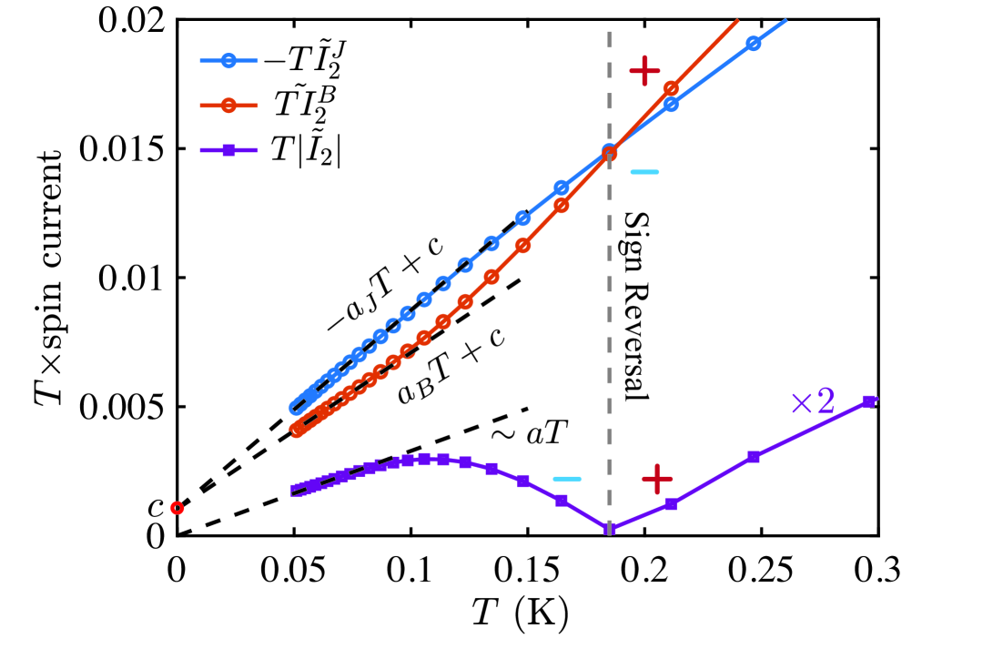
Figure 5: Simulated spin current and its components $\tilde{I}_{2}=\tilde{I}_{2}^{J}+\tilde{I}_{2}^{B}$, computed in the SSY phase under a magnetic field $B=0.05~{\rm T}$. The vertical gray dashed line indicates the location of sign reversal in net current $\tilde{I}_{2}$. The back dashed line shows the linear-fitting of the low-temperature $T\tilde{I}_{2}^{B,J}=a_{B,J}T\pm c$, with $a_{B}\simeq 0.061$, $a_{J}\simeq-0.077$, and $c\simeq 0.001$. The net spin current $T\tilde{I}_{2}$, values being amplified by twice in the plot, scales as $a\,T$ with $a=a_{B}+a_{J}\simeq 0.016$ at low temperature.

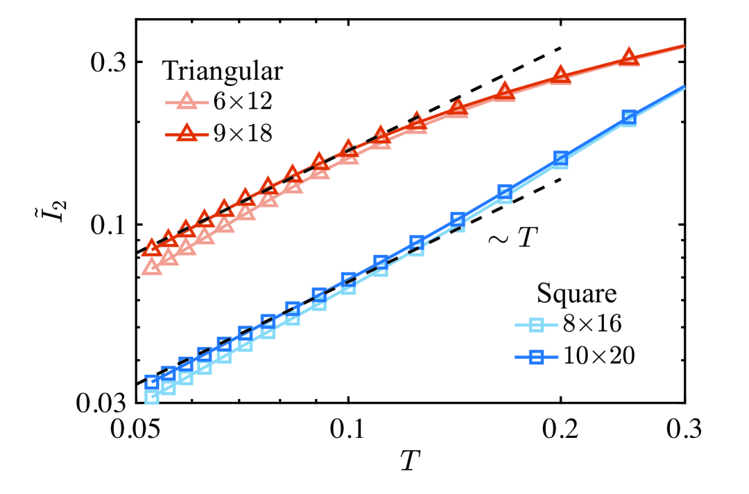
Figure 6: Simulated spin current $\tilde{I}_{2}$ of square- and triangular-lattice Heisenberg models at the QCPs ($B_{c}=4$ and $B_{c}=4.5$, respectively). The calculations are conducted on the $W\times L$ cylinder and the retained bond dimension is $D=2000$.

As $||\langle k|S_{j}^{-}|0\rangle||^{2}=||\frac{1}{\sqrt{N}}e^{ikj}||^{2}=\frac{1}{N}$ is a constant for any $k$, the quantity of interest, $X(\omega)$, can be represented as the density of states up to a constant. Based on Eq. (5), we have $X(\omega)\sim\omega^{\frac{d-z}{z}}$ in the low-frequency regime, where $d$ is the dimension of the system. Substitute it into the expression of $\tilde{I}_{S}=\int_{-\infty}^{\infty}d\omega~k^{2}(\beta\omega)X(\omega)$, we arrive at $\tilde{I}_{S}\sim T^{d/z}$. For 1D Heisenberg chain, this scaling reads $\tilde{I}_{S}\sim\sqrt{T}$, in consistent with the numerical results in Fig. 2(c). Beyond 1D chain, we further compute the spin current of 2D square- and triangular-lattice Heisenberg models at their polarized QCPs. As shown in Fig. 6, the low-temperature behavior exhibits a linear-$T$ scaling, i.e., $\tilde{I}_{S}\sim T$ ($d=z=2$).

Extended spin-current data in spin supersolids.— In Fig. 4, we demonstrated the persistent spin supercurrents in the SSY phase at 0.05 T, exhibiting temperature-independent supercurrent behavior mediated by the dissipationless Goldstone modes. Figure 7 extends these observations to wider field ranges, revealing persistent spin supercurrents in both the SSY phase (0.2 T) and SSV phase (1.3 T). Notably, all cases display a sign reversal from positive currents at high temperatures (UUD or paramagnetic phase) to negative currents in the supersolid regime. While the 0.05 T data shows clear low-temperature saturation, this behavior is observable in narrower temperature windows at 0.2 T and 1.3 T due to their lower supersolid transition temperatures. These findings robustly establish spin supercurrent SSE as an intrinsic signature of spin supersolid phases.

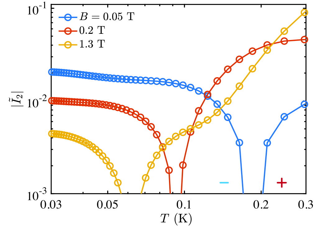
Figure 7: Simulated spin current $\tilde{I}_{2}$ for the TLAF model for NBCP. We show the simulated results for the 0.2 T case (SSY phase) and 1.3 T case (SSV phase), where the spin currents also exhibit sign reversal and temperature-independent saturation at low temperature. The $B=0.05$ T case that has been shown in the main text [Fig. 4(a)] is also plotted here as a comparison.

Linear spin-wave theory for spin current.— In the linear spin-wave theory (LSWT) calculations, we analyze the XXZ triangular-lattice model under fields. There are four phases, i.e., the SSY, UUD, SSV and the PL phases, separated by three quantum critical point $B_{c1,2,3}$. Since these spin states exhibit coplanar order, we constrain the magnetization to lie within the $x$-$z$ plane. To account for the three-sublattice structure, we employ Holstein-Primakoff transformations by introducing three bosonic operators $a_{1,2,3}$, corresponding to sublattices $A_{1,2,3}$, to parametrize the spin operators. We thus have

$$\begin{split}&S^{z}_{n}=\cos\theta_{n}~(S-a_{n}^{\dagger}a_{n})-\sin\theta_{n}~\frac{\sqrt{2S}}{2}(a_{n}+a_{n}^{\dagger}),\\ &S^{x}_{n}=\sin\theta_{n}~(S-a_{n}^{\dagger}a_{n})+\cos\theta_{n}~\frac{\sqrt{2S}}{2}(a_{n}+a_{n}^{\dagger}),\\ &S^{y}_{n}=\frac{\sqrt{2S}}{2i}(a_{n}-a_{n}^{\dagger}),\end{split}$$ (6)

where $\theta_{n}$ is determined by minimizing the classical energy

$$\begin{split}E=&\frac{S^{2}}{2}\sum_{n\neq n^{\prime}}\sin\theta_{n}\sin\theta_{n^{\prime}}+\frac{\Delta S^{2}}{2}\sum_{n\neq n^{\prime}}\cos\theta_{n}\cos\theta_{n^{\prime}}\\ &-\frac{BS}{3}\sum_{n}\cos\theta_{n}.\end{split}$$ (7)

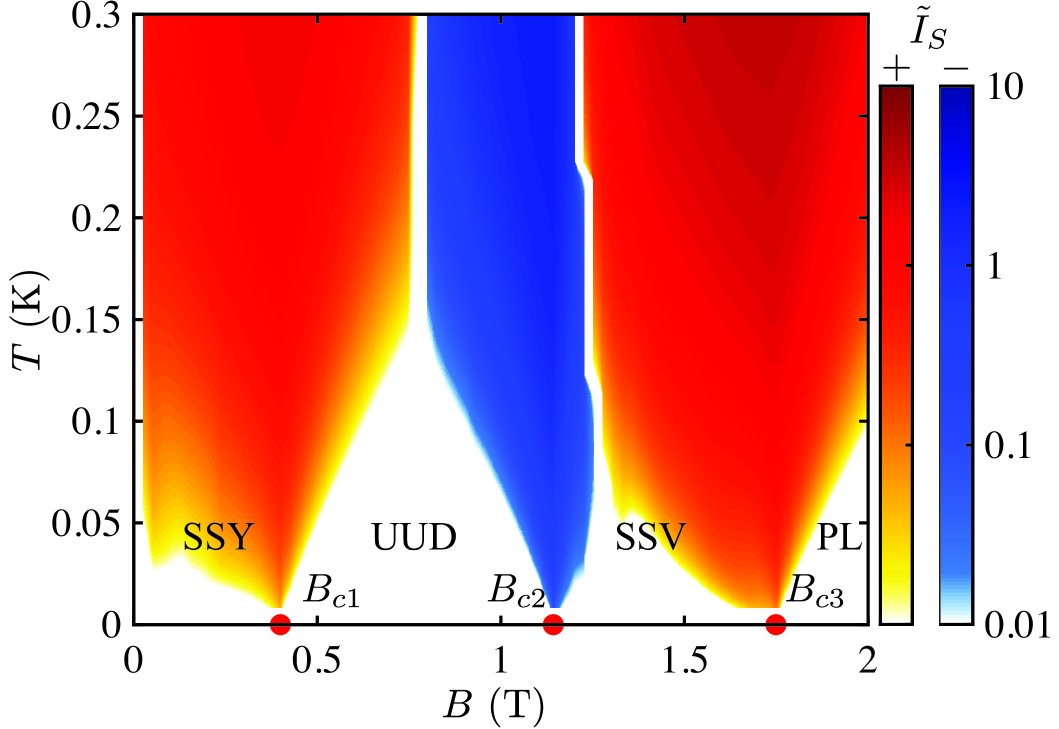
Figure 8: The LSWT results for the spin current $\tilde{I}_{S}$, which agree with tensor-network predictions in both the high-temperature regime and the low-temperature scaling near QCPs [see Fig. 3(a)], but fail to capture the persistent supercurrents observed in the supersolid phase. The SSY, UUD, SSV, and PL label the same quantum spin states as in Fig. 3(a), which are separated by three QCPs at $B_{c1,2,3}$. The red and blue color bars represent the positive and negative spin currents respectively.

By introducing the Fourier transformation and Bogoliubov transformation, we diagonalize the Hamiltonian in momentum space following as $H=\sum_{k}\beta_{k}^{\dagger}\hat{\lambda}_{k}\beta_{k}$ with $\beta_{k}^{\dagger}=(b_{1,k}^{\dagger},b_{2,k}^{\dagger},b_{3,k}^{\dagger},b_{1,-k},b_{2,-k},b_{2,-k})$ and $\hat{\lambda}_{k}=\text{diag}(\lambda_{1,k},\lambda_{2,k},\lambda_{3,k},-\lambda_{1,k},-\lambda_{2,k},-\lambda_{3,k})$.

Within the low-temperature regime where single-magnon excitations dominate, we compute the response function $X(\omega)$ to derive the spin current, with results shown in Fig. 8. In contrast to the tensor-network calculations of Fig. 4, the LSWT results in Fig. 8 reveal no negative spin current in either the SSY or SSV phases (see Supplementary Materials [58] for details). Instead, LSWT predicts exclusively positive currents that decay at low temperatures. This stark discrepancy underscores the necessity of beyond-LSWT methods — particularly the tensor-network approach with ITA developed here — to accurately capture these quantum spin transport phenomena.

Supplementary Materials for

Spin Seebeck Effect of Triangular-Lattice Spin Supersolid

Gao et al.

July 5, 2025

I Derivation of the normalized spin current

In this section, we show the detailed derivation of spin current in the spin Seebeck effect (SSE), i.e. Eq. (1) in the main text [48, 43, 57]. The full Hamiltonian describing the spin-metal junction can be expressed as

$$H=H_{S}+H_{M}+H_{\rm int}$$ (A1)

with

$$\begin{split}H_{S}&=\sum_{\langle i,j\rangle}\frac{J_{xy}}{2}(S_{i}^{+}S_{j}^{-}+S_{i}^{-}S_{j}^{+})+J_{z}S_{i}^{z}S_{j}^{z}-B\sum_{i}S_{i}^{z},\\ H_{M}&=\sum_{k,\sigma=\{\uparrow,\downarrow\}}\epsilon_{k,\sigma}f_{k,\sigma}^{\dagger}f_{k,\sigma},\\ H_{\rm int}&=J_{sd}\sum_{i\in{\rm int}}{S}_{i}\cdot{s}_{i},\end{split}$$ (A2)

where $\sum_{i\in{\rm int}}$ stands for the summation over all the sites on the interface, $S$ is the spin operator of the insulator quantum magnet and $s$ is the electron spin operator in the metal side.

The tunneling spin current is defined through the time derivative of the conduction electrons’ spin-polarization density at the interface:

$$I_{S}=\sum_{i\in{\rm int}}\frac{\partial}{\partial t}s_{i}^{z}(t)=-i\sum_{i\in{\rm int}}[s_{i}^{z}(t),H]=J_{sd}\sum_{i\in{\rm int}}-iS_{i}^{-}(t)s_{i}^{+}(t)+h.c.$$ (A3)

The statistical average of $I_{S}$ under the non-equilibrium steady state in the SSE experimental setup is given by

$$\langle I_{S}\rangle=2J_{sd}\sum_{i\in{\rm int}}{\rm Re}[(-i)\langle S_{i}^{-}(t)s_{i}^{+}(t)\rangle].$$ (A4)

Given the relative weakness of the $s-d$ coupling compared to the energy scales of both the metal and magnet, we treat $H_{S}$ and $H_{M}$ as unperturbed Hamiltonian while considering $H_{\rm int}$ as a perturbation. Assuming randomly distributed interface sites with inter-site distances significantly exceeding the lattice constants of both magnet and metal, we derive:

$$\langle I_{S}\rangle=2N_{\rm int}J_{sd}\lim_{\delta\rightarrow 0^{+}}{\rm Re}[F_{+-}^{<}(t,t^{\prime}=t+\delta)],$$ (A5)

where $F_{+-}^{<}(t,t^{\prime})=-i\langle S_{i}^{-}(t)s_{i}^{+}(t^{\prime})\rangle$ and $N_{\rm int}$ is the number of the interaction sites.

Expanding the exponential factor in the statistical average of $F_{+-}(t,t^{\prime})=-i\langle T_{C}s_{i}^{+}(t)S_{i}^{-}(t)\rangle$ with respect to $H_{\rm int}$:

$$\begin{split}F_{+-}(t,t^{\prime})&=-i\sum_{n=0}^{\infty}\frac{(-i)^{n}}{n!}\int_{C}dt_{1}\cdot\cdot\cdot\int_{C}dt_{n}\langle T_{C}\tilde{s}_{i}^{+}(t)\tilde{S}_{i}^{-}(t^{\prime})\tilde{H}_{\rm int}(t_{1})\cdot\cdot\cdot\tilde{H}_{\rm int}(t_{n})\rangle_{0}\\ &=(-i)^{2}\int_{C}dt_{1}\langle T_{C}\tilde{s}_{i}^{+}(t)\tilde{S}_{i}^{-}(t^{\prime})\tilde{H}_{\rm int}(t_{1})\rangle_{0}+\cdot\cdot\cdot,\end{split}$$ (A6)

where $\tilde{}$ stands for the time evolution under the unperturbed Hamiltonian, $\langle\cdot\cdot\cdot\rangle_{0}$ stands for the statistical average of the unperturbed Hamiltonian and $T_{C}$ is the time-ordered product on the Keldysh contour. Since the perturbed Hamiltonian is given by

$$\tilde{H}_{\rm int}(t_{1})=J_{sd}\sum_{i\in{\rm int}}\tilde{S}_{i}(t_{1})\cdot\tilde{s}_{i}(t_{1}),$$ (A7)

we have

$$\begin{split}F_{+-}(t,t^{\prime})&=J_{sd}\frac{(-i)^{2}}{2}\int_{C}dt_{1}\langle T_{C}\tilde{s}_{i}^{+}(t)\tilde{s}_{i}^{-}(t_{1})\rangle_{0}\langle T_{C}\tilde{S}_{i}^{+}(t_{1})\tilde{S}_{i}^{-}(t^{\prime})\rangle_{0}\\ &=\frac{J_{sd}}{2}\int_{C}dt_{1}~X_{+-}(t,t_{1})\chi_{+-}(t_{1},t^{\prime}),\end{split}$$ (A8)

where

$$\begin{split}X_{+-}(t,t^{\prime})&=-i\langle T_{C}\tilde{s}_{i}^{+}(t)\tilde{s}_{i}^{-}(t^{\prime})\rangle_{0}\\ \chi_{+-}(t,t^{\prime})&=-i\langle T_{C}\tilde{S}_{i}^{+}(t)\tilde{S}_{i}^{-}(t^{\prime})\rangle_{0}.\end{split}$$ (A9)

Using the Langreth rule, we have

$$F_{+-}^{<}(t,t^{\prime})=\frac{J_{sd}}{2}\int_{-\infty}^{\infty}dt_{1}[X_{+-}^{\rm R}(t,t_{1})\chi_{+-}^{<}(t_{1},t^{\prime})+X_{+-}^{<}(t,t_{1})\chi_{+-}^{A}(t_{1},t^{\prime})],$$ (A10)

with

$$\begin{split}X_{+-}^{\rm R}(t)&=-i\theta(t)\langle[\tilde{s}_{i}^{+}(t),{s}_{i}^{-}]\rangle_{0},\\ X_{+-}^{<}(t)&=-i\langle\tilde{s}_{i}^{-}(t)\tilde{s}_{i}^{+}\rangle_{0},\\ \chi_{+-}^{A}(t)&=i\theta(-t)\langle[\tilde{S}_{i}^{+}(t),\tilde{S}_{i}^{-}]\rangle_{0},\\ \chi_{+-}^{<}(t)&=-i\langle\tilde{S}_{i}^{-}(t)\tilde{S}_{i}^{+}\rangle_{0}.\end{split}$$ (A11)

Finally, applying the Fourier transformations, we arrive at

$$F_{+-}^{<}(t,t^{\prime})=\frac{J_{sd}}{4\pi}\int_{-\infty}^{\infty}d\omega~e^{-i\omega(t-t^{\prime})}[X_{+-}^{\rm R}(\omega)\chi_{+-}^{<}(\omega)+X_{+-}^{<}(\omega)\chi_{+-}^{A}(\omega)].$$ (A12)

Put Eq. (A12) into Eq. (A5), we have

$$\langle I_{S}\rangle=\frac{N_{\rm int}J_{sd}^{2}}{2\pi}\int_{-\infty}^{\infty}d\omega~{\rm Re}[X_{+-}^{\rm R}(\omega)\chi_{+-}^{<}(\omega)+X_{+-}^{<}(\omega)\chi_{+-}^{A}(\omega)].$$ (A13)

Considering the following relationship:

$$\begin{split}G^{<}(\omega)&=2i{\rm Im}[G^{\rm R}(\omega)]n(T),\\ G^{A}(\omega)&=G^{\rm R}(\omega)^{*},\\ n(T)&=\frac{1}{e^{\omega/T}-1},\end{split}$$ (A14)

we have

$$\begin{split}\langle I_{S}\rangle=&\frac{N_{\rm int}J_{sd}^{2}}{2\pi}\int_{-\infty}^{\infty}d\omega~{\rm Re}[2iX_{+-}^{\rm R}(\omega){\rm Im}[\chi_{+-}^{\rm R}(\omega)]n(T_{s})+2i{\rm Im}[X_{+-}^{\rm R}(\omega)]n(T_{m})\chi_{+-}^{\rm R}(\omega)^{*}]\\ =&\frac{N_{\rm int}J_{sd}^{2}}{\pi}\int_{-\infty}^{\infty}d\omega~-{\rm Im}[X_{+-}^{\rm R}(\omega)]{\rm Im}[\chi_{+-}^{\rm R}(\omega)]n(T_{s})+{\rm Im}[X_{+-}^{\rm R}(\omega)]{\rm Im}[\chi_{+-}^{\rm R}(\omega)]n(T_{m})\\ =&\frac{N_{\rm int}J_{sd}^{2}}{\pi}\int_{-\infty}^{\infty}d\omega~{\rm Im}[X_{+-}^{\rm R}(\omega)]{\rm Im}[\chi_{+-}^{\rm R}(\omega)](n(T_{m})-n(T_{s})).\end{split}$$ (A15)

We adopt the following approximations:

$$\begin{split}{\rm Im}[X_{+-}^{\rm R}(\omega)]\simeq&-a^{2}\omega,\\ n(T_{s})-n(T_{m})\simeq&\frac{\omega\delta T}{4T^{2}\sinh^{2}(\omega/(2T))},\end{split}$$ (A16)

where $a^{2}$ is a constant, $\delta T=T_{s}-T_{m}$ and $T=(T_{s}+T_{m})/2$. Note that $\chi_{+-}^{\rm R}(\omega)=-\chi_{-+}^{\rm R}(-\omega)$, we have

$$\begin{split}\langle I_{S}\rangle=&\frac{N_{\rm int}J_{sd}^{2}a^{2}\delta T}{4\pi T^{2}}\int_{-\infty}^{\infty}d\omega~{\rm Im}[\chi_{+-}^{\rm R}(\omega)]\frac{\omega^{2}}{\sinh^{2}(\beta\omega/2)}\\ =&-\frac{N_{\rm int}J_{sd}^{2}a^{2}\delta T}{4\pi}\int_{-\infty}^{\infty}d\omega~{\rm Im}[\chi_{-+}^{\rm R}(\omega)]\frac{(\beta\omega)^{2}}{\sinh^{2}(\beta\omega/2)}\\ =&-A\delta T\tilde{I}_{S},\end{split}$$ (A17)

where $A=\frac{1}{4\pi}N_{\rm int}J_{sd}^{2}a^{2}$ represents a material-dependent constant, $\delta T$ denotes the temperature gradient, $\beta\equiv 1/T$ is the inverse temperature, and the normalized spin current $\tilde{I}_{S}$ emerges as:

$$\tilde{I}_{S}=\int_{-\infty}^{\infty}d\omega~{\rm Im}[\chi_{-+}^{\rm R}(\omega)]\frac{(\beta\omega)^{2}}{\sinh^{2}(\beta\omega/2)}.$$ (A18)

Our present theoretical framework focuses on the intrinsic bulk properties through simulations of dynamical susceptibility and spin currents, aligning with Refs. [50, 57, 53]. In realistic setup, there are additional complexities due to interfacial disorder, electron tunneling effects, and edge contribution [52] — all of which must be properly accounted for when comparing with experiments.

II Imaginary time approximation for spin current

In this section, we present detailed derivation of the imaginary time approximation for the SSE. The spin current $I_{S}=-A\tilde{I}_{S}\delta T$ is induced by both the magnetic field and temperature gradient, where the normalized spin current $\tilde{I}_{S}$ is given by

$$\tilde{I}_{S}=\int_{-\infty}^{\infty}d\omega~k^{2}(\beta\omega){\rm Im}[\chi^{-+}_{\rm loc}(\omega)],$$ (B19)

with the dynamical susceptibility (retarded Green’s function)

$$\chi^{-+}_{\mathrm{loc}}(\omega)\equiv\chi_{-+}^{\rm R}(\omega)=-i\int_{0}^{\infty}~dt~\langle[S_{j}^{-}(t),S_{j}^{+}]\rangle_{T}e^{i\omega t},$$ (B20)

and $k^{2}(x\equiv\beta\omega)=x^{2}/\sinh^{2}{(x/2)}$. We assume that ${\rm Im}[\chi^{-+}_{\rm loc}(\omega)]$ is analytical near $\omega=0$, i.e.

$${\rm Im}[\chi^{-+}_{\rm loc}(\omega)]=\sum_{n=1}\frac{\omega^{n}}{n!}f_{n}.$$ (B21)

Since the integral kernel $k(x\equiv\beta\omega)=\frac{x}{\sinh(x/2)}$ is an even function of $\omega$, only the even terms in Eq. (B21) contribute. Given ${\rm Im}[\chi^{-+}_{\rm loc}(0)]=0$, we obtain

$$\begin{split}\tilde{I}_{S}&=\sum_{n=1}\int_{-\infty}^{\infty}d\omega~k^{2}(\beta\omega)\frac{\omega^{2n}}{(2n)!}f_{2n}\\ &=\sum_{n=1}\frac{1}{\beta^{2n+1}}\int_{-\infty}^{\infty}dx~k^{2}(x)\frac{x^{2n}}{(2n)!}f_{2n}\\ &=\sum_{n=1}\frac{F_{2n}}{\beta^{2n+1}}f_{2n}\\ &=\frac{16\pi^{4}}{15\beta^{3}}f_{2}+O(\frac{1}{\beta^{5}}),\end{split}$$ (B22)

where $F_{n}\equiv\int_{-\infty}^{\infty}dx~k^{2}(x)\frac{x^{n}}{n!}$.

Considering the relationship between the imaginary-time correlation function and dynamical susceptibility, i.e.

$$\langle S_{j}^{-}(\tau)S_{j}^{+}\rangle=-\frac{1}{\pi}\int_{-\infty}^{\infty}d\omega~\frac{e^{-\tau\omega}}{1-e^{-\beta\omega}}{\rm Im}[\chi_{\rm loc}^{-+}(\omega)],$$ (B23)

we have

$$\frac{\partial}{\partial\tau}\langle S_{j}^{-}(\tau)S_{j}^{+}\rangle=\frac{1}{\pi}\int_{-\infty}^{\infty}d\omega~\frac{\omega e^{-\tau\omega}}{1-e^{-\beta\omega}}{\rm Im}[\chi_{\rm loc}^{-+}(\omega)].$$ (B24)

Given $\tau=\beta/2$, we have

$$\begin{split}\frac{\partial}{\partial\tau}\langle S^{-}_{j}(\tau)S^{+}_{j}\rangle|_{\tau=\beta/2}&=\frac{1}{\pi}\int_{-\infty}^{\infty}d\omega~\frac{\omega e^{-\beta\omega/2}}{1-e^{-\beta\omega}}{\rm Im}[\chi_{\rm loc}^{-+}(\omega)]\\ &=\frac{1}{2\beta\pi}\int_{-\infty}^{\infty}d\omega~k(\beta\omega){\rm Im}[\chi_{\rm loc}^{-+}(\omega)]\\ &=\frac{1}{2\beta\pi}\sum_{n=1}\int_{-\infty}^{\infty}d\omega~k(\beta\omega)\frac{\omega^{2n}}{(2n)!}f_{2n}\\ &=\frac{1}{2\beta\pi}\sum_{n=1}\frac{1}{\beta^{2n+1}}\int_{-\infty}^{\infty}dx~k(x)\frac{x^{2n}}{(2n)!}f_{2n}\\ &=\frac{1}{2\beta\pi}\sum_{n=1}\frac{G_{2n}}{\beta^{2n+1}}f_{2n}\\ &=\frac{\pi^{3}}{\beta^{4}}f_{2}+O(\frac{1}{\beta^{6}}),\end{split}$$ (B25)

where $G_{n}\equiv\int_{-\infty}^{\infty}dx~k(x)\frac{x^{n}}{n!}$.

By comparing Eq. (B22) with Eq. (B25), we have

$$\tilde{I}_{S}=\frac{16\pi\beta}{15}\frac{\partial}{\partial\tau}\langle S_{j}^{-}(\tau)S_{j}^{+}\rangle|_{\tau=\beta/2}+O(\frac{1}{\beta^{5}})$$ (B26)

Thus at low temperature, we obtain the imaginary time approximation $\tilde{I}_{2}$ of the normalized spin current $\tilde{I}_{S}$ following as

$$\tilde{I}_{S}\sim\beta\frac{\partial}{\partial\tau}\langle S_{j}^{-}(\tau)S_{j}^{+}\rangle|_{\tau=\beta/2}.$$ (B27)

The correlation function derivation can be implemented through the following steps

$$\begin{split}\frac{\partial}{\partial\tau}\langle S_{j}^{-}(\tau)S_{j}^{+}\rangle=&\frac{1}{Z}{\rm Tr}[e^{-\beta H}e^{\tau H}HS_{j}^{-}e^{-\tau H}S_{j}^{+}-e^{-\beta H}e^{\tau H}S_{j}^{-}He^{-\tau H}S_{j}^{+}]\\ =&\frac{1}{Z}{\rm Tr}[e^{-\beta H}e^{\tau H}[H,S_{j}^{-}]e^{-\tau H}S_{j}^{+}]\\ =&\langle\mathcal{O}_{j}(\tau)S_{j}^{+}\rangle,\end{split}$$ (B28)

with $\mathcal{O}_{j}=[H,S_{j}^{-}]$. Finally, we arrive at

$$\tilde{I}_{2}\equiv\beta\langle\mathcal{O}_{j}(\frac{\beta}{2})S_{j}^{+}\rangle.$$ (B29)

III Tensor-network approach for finite-temperature spin dynamics

To compute the normalized spin current in Eq. (2) of the main text, we evaluate the finite-temperature local dynamical susceptibility (Eq. (B20)) using the real-time Green’s functions $g_{j}^{-+}(t)$ and $g_{j}^{+-}(t)$, defined as follows:

$$\begin{split}g_{j}^{-+}(t)&\equiv\langle S_{j}^{-}(t)S_{j}^{+}\rangle_{T}=\frac{1}{\mathcal{Z}}{\rm Tr}[e^{-\beta H}e^{iHt}S_{j}^{-}e^{-iHt}S_{j}^{+}]\\ g_{j}^{+-}(t)&\equiv\langle S_{j}^{+}(t)S_{j}^{-}\rangle_{T}=\frac{1}{\mathcal{Z}}{\rm Tr}[e^{-\beta H}e^{iHt}S_{j}^{+}e^{-iHt}S_{j}^{-}].\\ \end{split}$$ (C30)

Substituting them into Eq. (B20), the local susceptibility reads:

$$\begin{split}\chi_{\rm loc}^{-+}(\omega)=&-i\int_{0}^{\infty}dt~e^{i\omega t}(g_{j}^{-+}(t)-g_{j}^{+-}(-t))\\ =&\int_{0}^{\infty}dt~e^{i\omega t}({\rm Re}[g_{j}^{-+}(t)]+i{\rm Im}[g_{j}^{-+}(t)]-{\rm Re}[g_{j}^{+-}(t)]+i{\rm Im}[g_{j}^{+-}(t)])\\ =&\int_{0}^{\infty}dt~\sin(\omega t)({\rm Re}[g_{j}^{-+}(t)]-{\rm Re}[g_{j}^{+-}(t)])+\cos(\omega t)({\rm Im}[g_{j}^{-+}(t)]+{\rm Im}[g_{j}^{+-}(t)])\\ &+i\int_{0}^{\infty}dt~\cos(\omega t)({\rm Re}[g_{j}^{+-}(t)]-{\rm Re}[g_{j}^{-+}(t)])+\sin(\omega t)({\rm Im}[g_{j}^{-+}(t)]+{\rm Im}[g_{j}^{+-}(t)])\end{split}$$ (C31)

Noting that the kernel function is even in $\omega$, we retain only the even part of $\chi_{\mathrm{loc}}^{-+}(\omega)$, leading to:

$$\tilde{I}_{S}=2\int_{0}^{\infty}d\omega~k^{2}(\beta\omega)\int_{0}^{\infty}d\omega~\cos(\omega t){\rm Re}[g_{j}^{+-}(t)-g_{j}^{-+}(t)],$$ (C32)

with which the normalized spin current $\tilde{I}_{S}$ can be obtained by computing the real-time correlation ${\rm Re}[g_{j}^{+-}(t)-g_{j}^{-+}(t)]$.

We calculate the real-time correlation functions through three major steps:

• Construct the finite-temperature density matrix $\rho(\beta/2)=e^{-\beta H/2}$ using tanTRG [59];

• Compute the time-evolved state $\tilde{\rho}(t)=e^{-iHt}S_{j}^{+}\rho(\beta/2)e^{iHt}$ via time-dependent variational principle (TDVP) [60, 61];

• Evaluate the Green function $g_{j}^{-+}(t)={\rm Tr}[{\rho^{\dagger}(\beta/2)\tilde{\rho}(t)}]$ at each time step.

For the second step, while the original TDVP algorithm was formulated for matrix product states, it can be naturally generalized to MPO — see Ref. [59] for a concrete implementation.

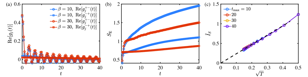
Figure S1: (a) Real part of the real-time Green’s function at different temperatures under a field of $B=B_{c}$ (QCP). (b) The entanglement entropy of the time-evolved state $\tilde{\rho}(t)$, sharing the same legend in (a). (c) The normalized spin current computed with different $t_{\rm max}$. In practical simulations, we evaluate the local Green’s function at the central site $j=64$ of $L=128$ chain, with retained bond dimension $D=500$.

Figure S1(a) displays the real-time Green’s functions of the 1D Heisenberg model simulated at the polarization QCP ($B_{c}=2$). The real component of $g_{j}^{+-}(t)$ exhibits significantly greater magnitude than that of $g_{j}^{-+}(t)$, with this disparity becoming increasingly pronounced at lower temperatures. This behavior is consistent with ground-state property, where $g_{j}^{-+}(t)$ strictly vanishes in the fully polarized state.

Figure S1(b) shows the time evolution of the purified entanglement entropy $S_{E}$. While $S_{E}$ grows during time evolution, a bond dimension of $D=500$ remains sufficiently large ($e^{\max(S_{E})}\approx 7.3891\ll 500$). This stands in sharp contrast to 2D systems, where the entanglement entropy of $rho(\beta/2)$ exhibits extensive scaling, making finite-temperature real-time evolution computationally intractable.

Figure S1(c) demonstrates improved low-temperature scaling with increasing $t_{\mathrm{max}}$, which is introduced in the computation of normalized spin current, i.e.,

$$\tilde{I}_{S}\simeq 2\int_{0}^{\infty}d\omega~k^{2}(\beta\omega)\int_{0}^{t_{\rm max}}d\omega~\cos(\omega t){\rm Re}[g_{j}^{+-}(t)-g_{j}^{-+}(t)].$$ (C33)

As the kernel function’s $k^{2}(\beta\omega)$ emphasis on low-frequency components at low temperatures, longer evolution time $t_{\mathrm{max}}$ is needed to capture the dominant low-frequency dynamics.

As a sanity check, we verify the accuracy of our real-time evolution by numerically comparing both sides of the equation

$$\beta\frac{\partial}{\partial\tau}\langle S^{-}_{j}(\tau)S^{+}_{j}\rangle\Big{|}_{\tau=\beta/2}=\frac{1}{2\pi}\int_{-\infty}^{\infty}d\omega\,k(\beta\omega)\,{\rm Im}[\chi_{\rm loc}^{-+}(\omega)],$$ (C34)

with $j=64$ at the center of the chain. In practice, we find the relative difference is below $4\times 10^{-4}$, indicating a well-converged real-time dynamical calculations with bond dimension $D=500$.

IV Analytical calculations of spinon spin current in 1D Tomonaga-Luttinger liquid

We consider the spin-$\frac{1}{2}$ Heisenberg spin chain with $J_{xy}=J_{z}=1$ as the energy unit. The normalized spin current is determined by the imaginary part of the local dynamical susceptibility. To compare with our numerical results, we consider the periodic boundary condition and the bulk contributions of the dynamical susceptibility to the spin currents. For a realistic experimental setup, the edge contribution may become nontrivial [52], and the competition between the edge and bulk contribution is not considered here.

For $0\leq B<2$ the ground state is the Tomonaga-Luttinger liquid (TLL) phase. Using the bosonized representation of the spin Hamiltonian, we arrive at a low-energy effective Hamiltonian given as [89]

$$\mathcal{H_{\text{eff}}}=\int dx\frac{v}{2}\{K^{-1}[\partial_{x}\phi(x)]^{2}+K[\partial_{x}\theta(x)]^{2}\}$$ (D35)

where $\phi(x)$ and $\theta(x)$ refer to the dual scalar fields, $K$ and $v$ refer to the TLL parameter and spinon velocity, respectively. The $\cos[\sqrt{16\pi}\phi(x)]$ term is irrelevant at finite magnetic fields [90], thus is ignored in Eq. (D35).

The TLL parameter $K$ is related to the compactification radius $R$ via $K=1/(4\pi R^{2})$ [89]. However, $R$ and $K$ are only explicitly solvable when $B=0$ and $2$. To obtain their values for $0<B<2$, we follow the procedure in Ref. [91]; also see the references within Ref. [91]. First, a dressed energy function $\varepsilon_{d}(\eta)$ is introduced and solved using the integral equation of

$$\varepsilon_{d}(\eta)=B-\frac{2}{\eta^{2}+1}-\frac{1}{2\pi}\int_{-\Lambda}^{\Lambda}\frac{4}{(\eta-\eta^{\prime})^{2}+4}\varepsilon_{d}(\eta^{\prime})d\eta^{\prime}$$ (D36)

where the real positive parameter $\Lambda$ is determined by the condition of $\varepsilon_{d}(\Lambda)=0$. In the limit of $B=0$, $\Lambda=\infty$, and for $B\ll 1$ an approximate expression is also given in Ref. [92]. After determining the value of $\Lambda$, a dressed charge function $\xi(\eta)$ is introduced as the solution of another integral equation given as

$$\xi(\eta)=1-\frac{1}{2\pi}\int_{-\Lambda}^{\Lambda}\frac{4}{(\eta-\eta^{\prime})^{2}+4}\xi(\eta^{\prime})d\eta^{\prime}$$ (D37)

where the compactification radius $R$ is determined by $R=1/(\sqrt{4\pi}\xi(\Lambda))$, or equivalently we can obtain $K=\xi(\Lambda)^{2}$.

Then, we turn to the dynamical spin susceptibility at finite temperatures. The large distance behavior of the dynamical spin susceptibility is carried out by combining the Bethe-Ansatz results and field theories. The spectral weight is most dominant when the momentum is near $\pi$ due to antiferromagnetic couplings. Following Ref. [50], the expression of the dynamical spin susceptibility $\chi^{-+}(\pi+q,\omega)$ is given as

$$\chi^{-+}(\pi+q,\omega)=\Theta(T,K)B(\frac{1}{8K}-i\frac{\omega-vq}{4\pi T},1-\frac{1}{4K})B(\frac{1}{8K}-i\frac{\omega+vq}{4\pi T},1-\frac{1}{4K})$$ (D38)

where $v$ is the spinon velocity and $\Theta(T,K)$ is determined by

$$\Theta(T,K)=-2A_{x}(K)\frac{(2-\frac{1}{K})\sin(\frac{\pi}{4K})}{\sin(\frac{\pi}{2K})}(\frac{\sin(\frac{\pi}{2K})}{2\pi T(2-\frac{1}{K})})^{2-\frac{1}{2K}}.$$ (D39)

In Eq. (D39), the nonuniversal amplitude $A_{x}(K)$ is related to $B_{0}(K)$ in Eq. (S6) of Ref. [50] by the equation of $A_{x}(K)=B_{0}^{2}(K)/2$ [90]; see more detailed expression of $A_{x}(K)$ in Ref. [93]. With Eq. (D38) we can obtain the temperature dependence of $\chi^{-+}(\pi+q,\omega)$, which is valid for small $q$, low energies $\omega$, and low temperatures $T$.

However, Eq. (D38) assumes the linear spinon dispersion with spinon velocity $v$. In this approximation ${\rm Im}[\chi^{-+}(\pi+q,\omega)]$ is an odd function of $\omega$, leading to a zero normalized spin current for any magnetic field. For larger magnetic fields, the nonlinear spinon dispersion becomes important in the excitation spectrum, and leads to some corrections to Eq. (D38). To fully consider the nonlinearity of the dispersions, one needs to start from the nonlinear TLL theory [94], which is beyond the scope of this paper. Here we follow the Supplementary Information of Ref. [50]. The linear terms $\pm vq$ in Eq. (D38) are replaced by the nonlinear dispersion $-\epsilon(\mp q)$, which is determined by the lower boundary of the spinon excitation continuum near $\pi$. The $\epsilon(q)$ under a finite magnetic field is given as [95]

$$\epsilon(q)=2[\frac{\pi}{2}+\frac{B}{2}(1-\frac{\pi}{2})]\cos(\frac{q}{2})\sin(\frac{q}{2}+\pi M)-B$$ (D40)

where $M=\frac{1}{\pi}\sin^{-1}(\frac{1}{1-\pi/2+\pi/B})$ is the approximate analytical expression for the magnetization associated with Eq. (D40).

Finally, the normalized spin current is calculated by integrating the imaginary part of the $\chi^{-+}(\pi+q,\omega)$ over $\omega$ and $q$. In practice, a cutoff $\omega_{\rm max}$ is introduced in the integration for calculations at low temperatures. Because of the kernel function in the formula for the spin current, we find that the integrand becomes neglectable for $\omega>\omega_{\rm max}$. For example, at $B=1$, for $T<0.01$ it is sufficient to choose $\omega_{\rm max}=0.2$. The local dynamical spin susceptibility is obtained by integrating over $q$. In our calculations, a cutoff $q_{\rm max}$ is also used and determined by the corresponding $\omega_{\rm max}$ in the spectrum to make sure that the dynamical spin susceptibility given in Eq. (D38) remains valid within the ranges.

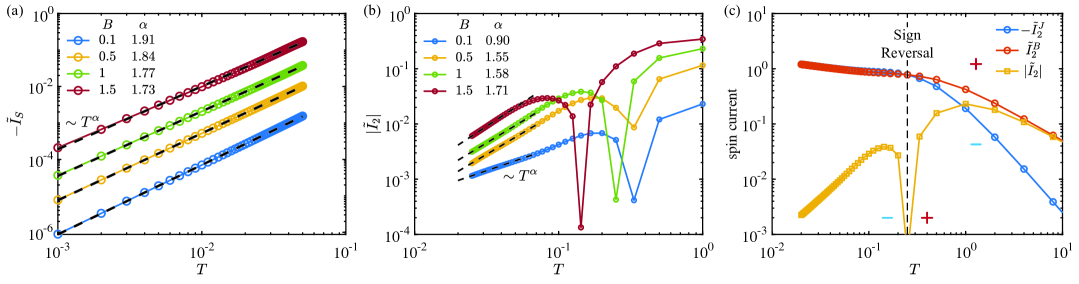
Figure S2: (a) Analytical result of the spin current $\tilde{I}_{S}$ at selected magnetic fields within the TLL regime. (b) Numerical result of the spin current $\tilde{I}_{2}$ at selected magnetic fields within the TLL regime. Black dashed lines indicate $T^{\alpha}$ power-law fits. (c) Simulated spin current and its components of 1D Heisenberg chain with $\tilde{I}_{2}=\tilde{I}_{2}^{J}+\tilde{I}_{2}^{B}$, computed under a magnetic field $B=1$. The vertical black dashed line indicates the location of sign reversal. A bond dimension of $D=500$ is retained in the calculations.

We show the temperature dependence of the spin current $\tilde{I}_{S}$ at finite magnetic fields in Fig. S2(a). The $\tilde{I}_{S}$ exhibits algebraic decay at low temperatures, which is consistent with our numerical results in the TLL phase. However, we notice that the exponent $\alpha$ is not exactly the same with the numerical calculations [see Fig. S2(b)], especially in the low magnetic field limit where higher orders of the nonlinear spinon dispersions cannot be ignored. In Fig. S2(c), we show the decomposition of spin current $\tilde{I}_{2}=\tilde{I}_{2}^{J}+\tilde{I}_{2}^{B}$, demonstrating sign reversal of net spinon spin current arise from the competition between interaction ($\tilde{I}_{2}^{J}$) and Zeeman-term ($\tilde{I}_{2}^{B}$) contributions.

V Sign Correspondence Between Spin Current and Magnetization Derivative

The spin current, defined as the flow of magnetization, arises in the SSE under a fixed temperature gradient. We find the spin current direction can be analyzed by checking the temperature response of the magnet’s total magnetization $M_{s}$, characterized by the derivative $\frac{dM_{s}}{dT}$. The total magnetization change along the magnetic sample can be expressed as $\delta M_{s}=-\delta T\cdot(\frac{dM_{s}}{dT})$, where $\delta T$ denotes the temperature difference across the magnet-metal interface. Through magnetization conservation between the magnet and metal layer, the magnetization change in the metal subtract is $\delta M_{s}=-\delta M_{m}$.

For the initial condition $T_{s}<T_{m}$ ($\delta T<0$) ensures $\delta M_{m}$ shares the sign of $-\frac{dM_{s}}{dT}$. This directly determines the spin current direction: outflow when $-\frac{dM_{s}}{dT}>0$ ($\delta M_{s}<0,\delta M_{m}>0$) or inflow when $-\frac{dM_{s}}{dT}<0$ ($\delta M_{s}>0,\delta M_{m}<0$). Figure S3(a) confirms such correspondence numerically, showing perfect alignment between the sign of $-\frac{dM_{s}}{dT}$ and the normalized current $\tilde{I}_{2}$, establishing the derivative as a robust predictor of current direction. The calculations are conducted on Y-type cylinder (of size YC$6\times 18$) as illustrated in Fig. S3(b).

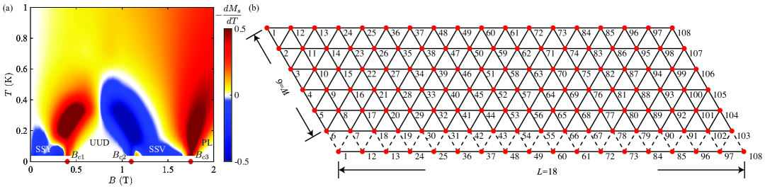
Figure S3: (a) Calculated $-\frac{dM_{s}}{dT}$ results for the realistic easy-axis TLAF model with $D=3000$. (b) The Y-type cylinder used in the calculation with width $W=6$ and length $L=18$ (YC$6\times 18$). The black dashed lines indicate the periodic boundary condition along $y$ axis. Magnetization $M$ is computed in the bulk region (19-90) to minimize finite-size effects.

VI Linear spin-wave study of spin Seebeck effect

Now we apply the linear spin-wave theory (LSWT) to the easy-axis triangular-lattice antiferromagnetic model with the Hamiltonian

$$H=J[\sum_{\langle i,j\rangle}S^{x}_{i}S^{x}_{j}+S^{y}_{i}S^{y}_{j}+\Delta S^{z}_{i}S^{z}_{j}-B\sum_{i}S_{i}^{z}],$$ (F41)

where $J$ is the energy scale and $\Delta$ is the anisotropic parameter. Under the linear spin wave approximation, the ground states of the model with $\Delta>1$ is a Y-shaped supersolid state (Y), a up-up-down solid state (UUD), a V-shaped supersolid state (V) and a polarized state, separating by three quantum critical point with

$$\begin{split}B_{c1}&=3S,\\ B_{c2}&=3S(\Delta-\frac{1}{2}+\sqrt{\Delta^{2}+\Delta-\frac{7}{4}}),\\ B_{c3}&=3S(1+2\Delta).\end{split}$$ (F42)

As all these state are (at least) coplanar state, we assume that the magnetization are on the $x$-$z$ plane. Considering the three sublattice order, we introduce three kinds of Holstein-Primakoff bosons $a_{1,2,3}$ on sublattices $A_{1,2,3}$ respectively to parametrize the spin operators. Generally speaking, we have

$$\begin{split}&S^{z}_{n}=\cos\theta_{n}~(S-a_{n}^{\dagger}a_{n})-\sin\theta_{n}~\frac{\sqrt{2S}}{2}(a_{n}+a_{n}^{\dagger}),\\ &S^{x}_{n}=\sin\theta_{n}~(S-a_{n}^{\dagger}a_{n})+\cos\theta_{n}~\frac{\sqrt{2S}}{2}(a_{n}+a_{n}^{\dagger}),\\ &S^{y}_{n}=\frac{\sqrt{2S}}{2i}(a_{n}-a_{n}^{\dagger}),\end{split}$$ (F43)

where $\theta_{n}$ can be obtained by minimizing classical energy

$$E=\frac{S^{2}}{2}\sum_{n\neq n^{\prime}}\sin\theta_{n}\sin\theta_{n^{\prime}}+\frac{\Delta S^{2}}{2}\sum_{n\neq n^{\prime}}\cos\theta_{n}\cos\theta_{n^{\prime}}-\frac{BS}{3}\sum_{n}\cos\theta_{n}.$$ (F44)

Now we consider the interactions between $n$ and $n^{\prime}$ site (only two operator terms):

$$\begin{split}S^{x}S^{x}:~&-S\sin\theta_{n}\sin\theta_{n^{\prime}}(a_{n}^{\dagger}a_{n}+a_{n^{\prime}}^{\dagger}a_{n^{\prime}})+\frac{S}{2}\cos\theta_{n}\cos\theta_{n^{\prime}}(a_{n}a_{n^{\prime}}+a_{n}a_{n^{\prime}}^{\dagger}+a_{n}^{\dagger}a_{n^{\prime}}+a_{n}^{\dagger}a_{n^{\prime}}^{\dagger}),\\ S^{y}S^{y}:~&-\frac{S}{2}(a_{n}a_{n^{\prime}}-a_{n}a_{n^{\prime}}^{\dagger}-a_{n}^{\dagger}a_{n^{\prime}}+a_{n}^{\dagger}a_{n^{\prime}}^{\dagger}),\\ \Delta S^{z}S^{z}:~&-S\Delta\cos\theta_{n}\cos\theta_{n^{\prime}}(a_{n}^{\dagger}a_{n}+a_{n^{\prime}}^{\dagger}a_{n^{\prime}})+\frac{S\Delta}{2}\sin\theta_{n}\sin\theta_{n^{\prime}}(a_{n}a_{n^{\prime}}+a_{n}a_{n^{\prime}}^{\dagger}+a_{n}^{\dagger}a_{n^{\prime}}+a_{n}^{\dagger}a_{n^{\prime}}^{\dagger}).\\ \end{split}$$ (F45)

By introducing the Fourier transformation $a_{n,i}=\frac{1}{\sqrt{N}}\sum_{k}e^{ikr_{n,i}}a_{n,k}$, we arrive at the quadratic Hamiltonian in momentum space $H_{k}=\sum_{k}\alpha_{k}^{\dagger}H_{0}(k)\alpha_{k}$, with $\alpha_{k}^{\dagger}=(a_{1,k}^{\dagger}~a_{2,k}^{\dagger}~a_{3,k}^{\dagger}~a_{1,-k}~a_{2,-k}~a_{3,-k})$.

Now we perform Bogoliubov transformation to diagonalize $H_{k}$, i.e., find a matrix $Q$ such that $(Q^{-1})^{\dagger}H_{0}(k)Q^{-1}=\hat{\lambda}\equiv\text{diag}[\lambda_{1},\lambda_{2},\lambda_{3},-\lambda_{1},-\lambda_{2},-\lambda_{3}]$. In order to maintain the Boson commutation relation after the transformation $\beta_{k}=Q\alpha_{k},\beta_{k}^{\dagger}=(b_{1,k}^{\dagger}~b_{2,k}^{\dagger}~b_{3,k}^{\dagger}~b_{1,-k}~b_{2,-k}~b_{3,-k})$, $Q$ needs to satisfy $QLQ^{\dagger}=Q^{\dagger}LQ=L$, $Q^{\dagger}L=LQ^{-1}$, with $L=\text{diag}[1,1,1,-1,-1,-1]$. Numerically, one can use the following step to obtain $Q$:

• Find $K$ such that $H_{0}(k)=K^{\dagger}K$;

• Diagonalize $KLK^{\dagger}$ with unitary matrix $U$ such that $U^{\dagger}(KLK^{\dagger})U=\hat{\lambda}$;

• Obtain the eigenvalue $\lambda=L\hat{\lambda}$;

• Obtain the transfer matrix $Q=(\sqrt{\lambda})^{-1}U^{\dagger}K$.

Within the one-magnon space, we can obtain the local dynamical susceptibility as follow

$$\begin{split}\frac{1}{2}{\rm Im}[\chi^{-+}_{\rm loc}(\omega)+\chi^{-+}_{\rm loc}(-\omega)]&=\frac{\pi}{2\mathcal{Z}}\sum_{m,n}(||\langle m|S_{j}^{-}|n\rangle||^{2}-||\langle m|S_{j}^{+}|n\rangle||^{2})e^{-\beta E_{n}}(1-e^{-\beta\omega})\delta(\omega+E_{n}-E_{m})\\ &\simeq\frac{\pi}{2N}\sum_{m,k,i}(||\langle 0|b_{i,k}S_{k}^{-}|0\rangle||^{2}-||\langle 0|b_{i,k}S_{k}^{+}|0\rangle||^{2})(1-e^{-2\beta\lambda_{i}})\delta(\omega-2\lambda_{i}),\end{split}$$ (F46)

with $S_{k}^{+}=\sum_{i=1}^{3}\frac{1}{2}\cos\theta_{n}(a_{i,k}+a_{i,k}^{\dagger})+\frac{1}{2}(a_{i,k}-a_{i,k}^{\dagger})$, $a_{j,k}=\sum_{l=1}^{3}P_{j,l}b_{l,k}+\sum_{l=1}^{3}P_{j,l+3}b_{l,-k}^{\dagger}$, and $P=Q^{-1}$. Thus we have $\langle 0|b_{i,k}a_{j,k}|0\rangle=P_{j,i+3}$, $\langle 0|b_{i,k}a_{j,k}^{\dagger}|0\rangle=P_{j,i}^{*}$, and

$$\begin{split}||\langle 0|b_{i,k}S_{k}^{+}|0\rangle||^{2}&=||\langle 0|b_{i,k}\sum_{l=1}^{3}\frac{1}{2}(\cos\theta_{l}+1)a_{l,k}+\frac{1}{2}(\cos\theta_{l}-1)a_{l,k}^{\dagger}|0\rangle||^{2}\\ &=||\sum_{l=1}^{3}\frac{1}{2}(\cos\theta_{l}+1)P_{l,j+3}+\frac{1}{2}(\cos\theta_{l}-1)P_{l,j}^{*}||^{2};\\ ||\langle 0|b_{i,k}S_{k}^{-}|0\rangle||^{2}&=||\langle 0|b_{i,k}\sum_{l=1}^{3}\frac{1}{2}(\cos\theta_{l}-1)a_{l,k}+\frac{1}{2}(\cos\theta_{l}+1)a_{l,k}^{\dagger}|0\rangle||^{2}\\ &=||\sum_{l=1}^{3}\frac{1}{2}(\cos\theta_{l}-1)P_{l,j+3}+\frac{1}{2}(\cos\theta_{l}+1)P_{l,j}^{*}||^{2}.\end{split}$$ (F47)

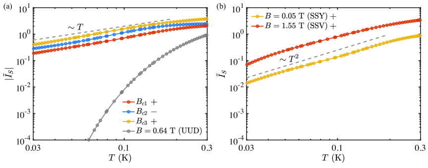
Figure S4: The LSWT results for the spin current $\tilde{I}_{S}$ under applied magnetic fields. (a) Behavior across three critical fields and in the UUD phase; (b) Results in the SSY and SSV supersolid phases. The “$+$” and “$-$” sign represent the positive and negative spin current, respectively.

By substituting Eq. (F47) into Eq. (F46), we compute $\tilde{I}_{S}$ within LSWT (Fig. S4). While the linear-$T$ behavior at QCPs agrees with tensor-network results in the main text (Fig. 3(c)), LSWT exhibits significant limitations in the supersolid phase. Specifically, it predicts a $T^{2}$ temperature dependence [Fig. S4(b)] rather than the persistent currents observed in tenso-network numerical simulations, and produces exclusively positive currents in both SSY and SSV phases — in stark contrast to the behavior shown in Fig. 4(a). These discrepancies clearly indicate that investigating spin currents in supersolid systems necessitates theoretical approaches that go beyond conventional LSWT.