QCD sum rule analysis of $J^{PC}=1^{--}$ light hybrid mesons

Abstract

We performed a comprehensive next-to-leading order (NLO) QCD sum rule analysis of the light hybrid meson with quantum numbers $J^{PC}=1^{--}$. Utilizing both Laplace sum rules (LSR) and Gaussian sum rules (GSR), we investigate the two-point correlation function of the light hybrid interpolating current, including condensates up to dimension-8. A conservative range $2-2.5\text{GeV}$ is obtained. Notably, the GSR yield mass predictions $2.27\text{GeV}$ for the $s\bar{s}g$ and $2.19\text{GeV}$ for $u\bar{u}g$. This result is notably lower than many previous sum rule estimates and significantly reduces the discrepancy with predictions from lattice QCD and flux-tube models. This result revitalizes the interpretation of the $\phi(2170)$ resonance as a possible candidate for the light vector hybrid meson.

1 Introduction

Non-$q\bar{q}$ mesons play an important role in modern hadron spectroscopy. Quantum Chromodynamics (QCD) permits states in which gluons act as structural constituents. These hybrid mesons ($q\bar{q}g$) provide a testing ground for studying hadron structure, confinement, and the non-perturbative aspects of QCD.

While research on hybrids often focuses on states with exotic $J^{PC}$ quantum numbers (e.g., $0^{+-}$, $1^{-+}$, $2^{+-}$) that are forbidden for conventional $q\bar{q}$ mesons, hybrids with conventional quantum numbers are also intriguing. For the$J^{PC}=1^{--}$ hybrid, the flux-tube model predicts masses of $1.8-1.9\text{GeV}$ for $u\bar{u}g$ and $2.1-2.2\text{GeV}$ for $s\bar{s}g$  [1--_flux_tube]. In contrast, QCD sum rule calculations have consistently yielded heavier masses, with early estimates for the $s\bar{s}g$ hybrid around $2.9\text{GeV}$ [1--_LSR_weyers, 1--_GSR_chen] and a more recent study providing a mass of $2.5\text{GeV}$ [1--_LSR_sundu]. Lattice QCD results fall in between, placing the isovector hybrid at $2.2-2.3\text{GeV}$ and its isoscalar partner at $2.4-2.5\text{GeV}$ [1--_lattice_dudek]. Another lattice study noted a potential candidate near $2.1-2.3\text{GeV}$, but could not confirm its nature due to possible contamination from higher energy states [1--_lattice_liu].

Experimentally, the most prominent candidate for a strangeonium-like $1^{--}$ hybrid is the $\phi(2170)$ resonance, also known as $Y(2175)$. This state was first observed by the BaBar collaboration [phi_2170_babar_06] in the $e^{+}e^{-}\rightarrow\phi(1020)f_{0}(980)$ process and subsequently confirmed by other experiments [phi_2170_babar_08, phi_2170_bes_08, phi_2170_belle_09, phi_2170_bes3_19] through various production mechanisms and decay modes. The Particle Data Group (PDG) [pdg] currently lists its world-average mass as $2164\pm 6\text{MeV}$ and its width as $106_{-18}^{+24}\text{MeV}$. It has been observed decaying mainly into final states containing a $s\bar{s}$ pair, such as $\phi f_{0}(980)$, $\phi\pi^{+}\pi^{-}$, and $\phi\eta$.

The substantial discrepancy between the experimental mass and QCD sum rule predictions has led to controversy regarding the internal structure of $\phi(2170)$. The $\phi(2170)$ has also been explored as a tetraquark state [1--_tetra_chen, 1--_tetra_lebed], a $\Lambda\bar{\Lambda}$ molecular state [1--_mole_valery, 1--_mole_li], a $\phi K\bar{K}$ system or $\phi f_{0}(980)$ molecule [1--_phif0_KP, 1--_phif0_mart], or a conventional excited $s\bar{s}$ meson [1--_ssbar_page, 1--_ssbar_yan]. While each of these alternative scenarios is supported by theoretical arguments and experimental observations, they also face difficulties in fully explaining the particle’s mass and decay properties.

In this paper, we perform a comprehensive next-to-leading order (NLO) analysis of the $1^{--}$ hybrid meson. Using both Laplace sum rules (LSR) [qsr] and Gaussian sum rules (GSR) [gaussian], the conservative mass prediction is in the range of $2-2.5\text{GeV}$, while GSR fitting gives preciser mass predictions (with standard error): $2.27\pm 0.01\text{GeV}$ for the $s\bar{s}g$ hybrid and $2.19\pm 0.14\text{GeV}$ for $u\bar{u}g$. This result significantly narrows the gap between QCD sum rule predictions and those from other theoretical approaches, and brings the predicted mass closer to that of the $\phi(2170)$, suggesting that the $1^{--}$ light hybrid is a plausible interpretation within the QCD sum rule framework.

2 QCD Sum Rules of $1^{--}$ Hybrid

Figure 1: The perturbative diagrams, including the diagrams from counterterms.

For the $1^{--}$ hybrid meson, the interpolating current as [1--_LSR_weyers, 1--_GSR_chen]:

$$J^{\mu}=\overline{\Psi}\gamma_{\rho}.\gamma^{5}T^{n}\widetilde{G}^{n\,\rho\mu}\Psi;\qquad\widetilde{G}^{n\,\rho\mu}=\varepsilon^{\rho\mu\alpha\beta}G^{n}_{\alpha\beta};\qquad\varepsilon^{0123}=1.$$ (1)

Here, $T^{n}$ are the color matrices. The mass of the corresponding hybrid can be derived from the correlator:

$$\Pi^{\mu\nu}(q^{2})=i\int dx\,e^{-iqx}\langle TJ^{\mu}(x)J^{\dagger\,\nu}(0)\rangle=\Big{(}\frac{q^{\mu}q^{\nu}}{q^{2}}-g^{\mu\nu}\Big{)}\Pi_{v}(q^{2})+\frac{q^{\mu}q^{\nu}}{q^{2}}\Pi_{s}(q^{2}),$$ (2)

where the sign of polarization tensor $\frac{q^{\mu}q^{\nu}}{q^{2}}-g^{\mu\nu}$ is fixed by requiring $\text{Im}\Pi_{v}(s)>0$ as $s\rightarrow\infty$. The vector part, $\Pi_{v}(q^{2})$, contains the information about the $1^{--}$ hybrid state.

Utilizing operator-product-expansion (OPE), our calculation incorporates condensates up to dimension-8. The perturbative, $\langle GG\rangle$, and $\langle\bar{q}q\rangle^{2}$ diagrams are calculated to next-to-leading order (NLO), see figures 1, 2, and 3. The renormalization of hybrid current, other relevant diagrams, and necessary technical details are presented in Appendices A and B. The renormalized $1^{--}$ hybrid current yields:

$$\split\Pi_{v}(q^{2})=&-\log\!\Big{(}\!\!-\!\frac{q^{2}}{\mu^{2}}\Big{)}\bigg{[}\frac{(6n_{f}-35)\alpha_{s}^{2}q^{6}}{4320\pi^{4}}\log\!\Big{(}\!\!-\!\frac{q^{2}}{\mu^{2}}\Big{)}-\frac{(454n_{f}-6815)\alpha_{s}^{2}q^{6}}{43200\pi^{4}}+\frac{\alpha_{s}q^{6}}{60\pi^{3}}\bigg{]}\\ &+\!\bigg{[}\frac{8\alpha_{s}q^{2}}{81\pi^{2}}\log\!\Big{(}\!\!-\!\frac{q^{2}}{\mu^{2}}\Big{)}-\frac{17\alpha_{s}q^{2}}{216\pi^{2}}+\frac{q^{2}}{9\pi}\bigg{]}\log\!\Big{(}\!\!-\!\frac{q^{2}}{\mu^{2}}\Big{)}\langle GG\rangle-\!\frac{16\alpha_{s}}{9\pi}q^{2}\log\!\Big{(}\!\!-\!\frac{q^{2}}{\mu^{2}}\Big{)}m\!\left\langle\overline{\Psi}\Psi\text{}\right\rangle\\ &+\frac{2}{81}(24n_{f}\!+\!103)\alpha_{s}^{2}\log\!\Big{(}\!\!-\!\frac{q^{2}}{\mu^{2}}\Big{)}\!\left\langle\overline{\Psi}\Psi\text{}\right\rangle^{2}\!\!-\!\frac{16}{27}\alpha_{s}^{2}\log\!\Big{(}\!\!-\!\frac{q^{2}}{\mu^{2}}\Big{)}\big{[}\!\left\langle\bar{u}u\text{}\right\rangle^{2}\!\!+\!\left\langle\bar{d}d\text{}\right\rangle^{2}\!\!+\!\left\langle\bar{s}s\text{}\right\rangle^{2}\!\big{]}\\ &+\frac{15}{8\pi}\alpha_{s}\log\!\Big{(}\!\!-\!\frac{q^{2}}{\mu^{2}}\Big{)}m\!\left\langle\overline{\Psi}G\Psi\text{}\right\rangle-\frac{154\pi\alpha_{s}}{27q^{2}}\left\langle\overline{\Psi}\Psi\text{}\right\rangle\left\langle\overline{\Psi}G\Psi\text{}\right\rangle,$$ (3)

and

$$\split\Pi_{s}(q^{2})=&-\log\!\Big{(}\!\!-\!\frac{q^{2}}{\mu^{2}}\Big{)}\bigg{[}\frac{\left(6n_{f}-35\right)\alpha_{s}^{2}q^{6}}{8640\pi^{4}}\log\!\Big{(}\!\!-\!\frac{q^{2}}{\mu^{2}}\Big{)}-\frac{\left(1722n_{f}-20945\right)\alpha_{s}^{2}q^{6}}{259200\pi^{4}}+\frac{\alpha_{s}q^{6}}{120\pi^{3}}\bigg{]}\\ &-\!\bigg{[}\frac{4\alpha_{s}q^{2}}{27\pi^{2}}\log\!\Big{(}\!\!-\!\frac{q^{2}}{\mu^{2}}\Big{)}-\frac{115\alpha_{s}q^{2}}{432\pi^{2}}+\frac{q^{2}}{6\pi}\bigg{]}\log\!\Big{(}\!\!-\!\frac{q^{2}}{\mu^{2}}\Big{)}\langle GG\,\rangle-\!\frac{4\alpha_{s}}{3\pi}q^{2}\log\!\Big{(}\!\!-\!\frac{q^{2}}{\mu^{2}}\Big{)}m\!\left\langle\overline{\Psi}\Psi\text{}\right\rangle\\ &+\frac{74}{81}\alpha_{s}^{2}\log\!\Big{(}\!\!-\!\frac{q^{2}}{\mu^{2}}\Big{)}\left\langle\overline{\Psi}\Psi\text{}\right\rangle^{2}+\frac{16}{27}\alpha_{s}^{2}\log\!\Big{(}\!\!-\!\frac{q^{2}}{\mu^{2}}\Big{)}\big{[}\left\langle\bar{u}u\text{}\right\rangle^{2}+\left\langle\bar{d}d\text{}\right\rangle^{2}+\left\langle\overline{\Psi}\Psi\text{}\right\rangle^{2}\big{]}\\ &-\frac{15}{8\pi}\alpha_{s}\log\!\Big{(}\!\!-\!\frac{q^{2}}{\mu^{2}}\Big{)}m\!\left\langle\overline{\Psi}G\Psi\text{}\right\rangle+\frac{92\pi\alpha_{s}}{27q^{2}}\left\langle\overline{\Psi}\Psi\text{}\right\rangle\left\langle\overline{\Psi}G\Psi\text{}\right\rangle.$$ (4)

Figure 2: Diagrams corresponding to $\langle GG\rangle$, including diagrams from counterterms.

Figure 3: Diagrams corresponding to $\langle qq\rangle^{2}$.

Here, terms that do not contribute to the imaginary part have been omitted; $n_{f}=3$ is adopted for mass estimation. The $\langle\bar{u}u\text{}\rangle^{2}+\langle\bar{d}d\text{}\rangle^{2}+\langle\bar{s}s\text{}\rangle^{2}$ terms originate from gluon equation of motion, and

$$\langle GG\rangle=\langle\alpha_{s}G^{n}_{\mu\nu}G^{n\,\mu\nu}\rangle,\qquad\langle\bar{s}Gs\rangle=\langle\bar{s}g\sigma^{\mu\nu}T^{n}G^{n}_{\mu\nu}s\rangle,\quad\sigma^{\mu\nu}=\frac{i}{2}[\gamma^{\mu},\gamma^{\nu}].$$ (5)

Through the dispersion relation [qcd_book, qsr, qsr_intro_2, qsr_book], the correlator can be related to the spectral function. Under the “pole $+$ continuum” ansatz, the dispersion relation yields

$$\frac{1}{\pi}\text{Im}\Pi(s)=f^{2}\delta(s-m^{2})+\theta(s-s_{0})\rho(s),$$ (6)

where $m$ is the mass of the lowest-lying resonance, $s_{0}$ is the continuum threshold, and $\rho(s)$ is the continuum spectral density.

For the numerical analysis, we use the following quark masses [pdg] and condensate values [qcd_sum_review] (both at $\mu=2\text{GeV}$):

$$\split m_{u}&=2.16\text{MeV},\quad m_{d}=4.70\text{MeV},\quad m_{s}=93.5\text{MeV},\quad\langle\bar{q}q\rangle=-(0.276)^{3}\text{GeV}^{3},\\ \langle\bar{s}s\rangle&=0.8\langle\bar{q}q\rangle,\quad\langle GG\rangle=0.07\text{GeV}^{4},\quad\langle\bar{s}Gs\rangle=0.8\text{GeV}^{2}\times\langle\bar{s}s\rangle,$$ (7)

where $q=u,d$. The value of $\langle\bar{q}q\rangle$ corresponds to applying GMOR relation [Chpt_scholarpedia]

$$-(m_{u}+m_{d})\langle\bar{u}u\rangle=f^{2}_{\pi}m_{\pi}^{2}$$ (8)

to the quark masses at $\mu=2\text{GeV}$.

The one-loop approximation of running $\alpha_{s}$ is used:

$$\alpha_{s}(\mu^{2})=\frac{\alpha_{s}(m^{2}_{\tau})}{1+\frac{\beta_{0}}{4\pi}\alpha_{s}(m^{2}_{\tau})\log\big{(}\frac{\mu^{2}}{m^{2}_{\tau}}\big{)}},$$ (9)

where [pdg]

$$m_{\tau}=1776.93\pm 0.09\text{MeV},\qquad\alpha_{s}(m^{2}_{\tau})=0.314\pm 0.014,$$ (10)

and $\beta_{0}=9$ for $n_{f}=3$.

2.1 Laplace Sum Rules

The Laplace sum rule (LSR) method involves applying Borel transformation [qcd_book, qsr, qsr_intro_2] to the correlation function. This procedure eliminates subtraction terms from the dispersion relation [qsr, qsr_intro_2] and exponentially suppresses contributions from higher states and the continuum, thereby isolating the contribution of the lowest-lying resonance. Applying the Borel transformation to the moments of spectral functions yields:

$$\mathcal{M}^{n}(\tau,s_{0})=\frac{1}{\pi}\int_{0}^{s_{0}}ds\ s^{n}e^{-\tau s}\,\text{Im}\Pi_{v}(s)=f^{2}m^{2n}e^{-\tau m^{2}},$$ (11)

where $\tau$ is the Borel parameter; the renormalization group improved moments are obtained by setting $\mu^{2}\rightarrow 1/\tau$ [qsr_laplace]. The mass of the lowest resonance can then be extracted from the ratio of these moments:

$$\mathcal{R}^{n}(\tau,s_{0})=\frac{\mathcal{M}^{n+1}(\tau,s_{0})}{\mathcal{M}^{n}(\tau,s_{0})}=m^{2}.$$ (12)

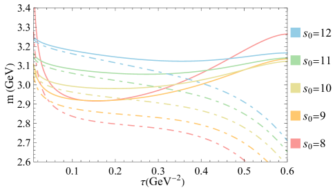
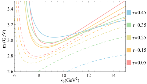
Figure 4: Leading order results for $\sqrt{\mathcal{R}^{0}}$ versus $\tau(\text{GeV}^{-2})$ and $s_{0}(\text{GeV}^{2})$. Dot-dashed line corresponding to $u\bar{u}g$; solid lines corresponding to $s\bar{s}g$.

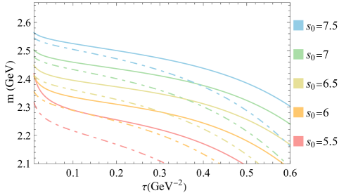
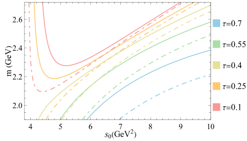
Figure 5: Next-to-Leading Order results for $\sqrt{\mathcal{R}^{0}}$ versus $\tau(\text{GeV}^{-2})$ and $s_{0}(\text{GeV}^{2})$. Dot-dashed line corresponding to $u\bar{u}g$; solid lines corresponding to $s\bar{s}g$.

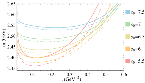
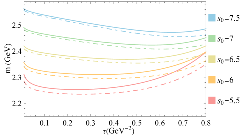
Figure 6: $\sqrt{\mathcal{R}^{n}}$ versus $\tau(\text{GeV}^{-2})$ with dimension-8 condensate has been excluded. The left plot shows $\sqrt{\mathcal{R}^{0}}(\tau)$; the right plot shows $\sqrt{\mathcal{R}^{1}}(\tau)$. Dot-dashed line corresponding to $u\bar{u}g$; solid lines corresponding to $s\bar{s}g$.

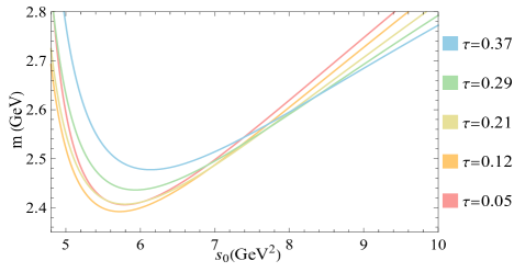
(a) $\sqrt{\mathcal{R}^{0}}(s_{0})$ for $s\bar{s}g$.

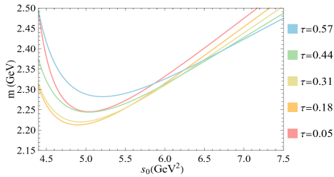
(b) $\sqrt{\mathcal{R}^{1}}(s_{0})$ for $s\bar{s}g$.

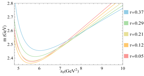
(c) $\sqrt{\mathcal{R}^{0}}(s_{0})$ for $u\bar{u}g$.

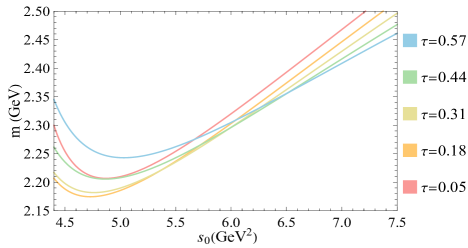
(d) $\sqrt{\mathcal{R}^{1}}(s_{0})$ for $u\bar{u}g$.

Figure 7: $\sqrt{\mathcal{R}^{n}}$ versus $s_{0}(\text{GeV}^{2})$, with dimension-8 condensate has been excluded.

Based on equation. 3, we present the leading order results in figure 4. The estimated masses are around $3\text{GeV}$, which reproduce the results in previous works [1--_LSR_weyers, 1--_GSR_chen], but does not agree with the result in Ref [1--_LSR_sundu] ($\simeq 2.5\text{GeV}$). The later is obtained from LO calculation that incorporates condensates up to dimension-10.

As shown in figure 5, the NLO results are much lower then LO results, however, the $\tau$-stability disappeared and extracting the mass becomes difficult. Nevertheless, the curve is nearly stable around $\tau\approx 0.2\,\text{GeV}^{-2}$ and $s_{0}\approx 7\,\text{GeV}^{2}$, which suggests a mass $\approx 2.4\,\text{GeV}$.

If we exclude the dimension-8 condensate, the stability of the LSR improves. As shown in figures 6 and 7, the predicted mass is around $2.2-2.5\,\text{GeV}$. Here, we use both $\sqrt{\mathcal{R}^{0}}$ and $\sqrt{\mathcal{R}^{1}}$ to extract the mass. We observe that $\sqrt{\mathcal{R}^{1}}$ exhibits better $\tau$-stability but worse $s_{0}$-stability, whereas $\sqrt{\mathcal{R}^{0}}$ shows the opposite behavior. For all the cases, the mass of $u\bar{u}g$ is lower than the mass of $s\bar{s}g$ as anticipated, but the exact mass difference is difficult to estimate.

Compared to leading-order (LO) predictions in figure 4 and in Refs [1--_LSR_weyers, 1--_GSR_chen], which placed the mass $\approx 2.9\,\text{GeV}$, the NLO analysis significantly lowers the predicted mass by roughly $0.4-0.7\,\text{GeV}$, indicating the importance of NLO correction.

2.2 Gaussian Sum Rules

The Gaussian sum rule (GSR) [gaussian, gsr_bayesian] enables a more detailed examination of the hadronic spectral function. The GSR employs a Gaussian kernel, $e^{-(s-t)^{2}/4\tau}$, which focuses on a specific region of the spectrum. By varying the center of this kernel, one can, in principle, probe different regions of the spectrum and study excited states. Moreover, the GSR utilizes a fitting procedure to extract hadron properties, which reduces the bias from the choice of the continuum threshold $s_{0}$, and yields a more robust prediction.

The GSR of the $1^{--}$ hybrid is defined as:

$$G(\tau,s,s_{0})=\frac{1}{\sqrt{4\pi\tau}}\int_{0}^{s_{0}}dt\,e^{-\frac{(s-t)^{2}}{4\tau}}\frac{1}{\pi}\text{Im}\Pi_{v}(t).$$ (13)

On the hadron side, applying the Gaussian transformation to the “pole $+$ continuum” ansatz yields:

$$G_{h}(\tau,s)=\frac{f^{2}}{\sqrt{4\pi\tau}}e^{-\frac{(s-m^{2})^{2}}{4\tau}}.$$ (14)

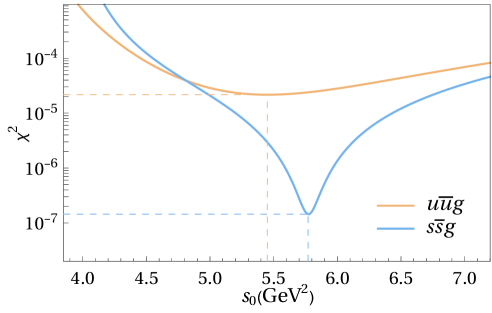
(a) Minimized $\chi^{2}$ versus $s_{0}$.

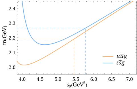
(b) Fitted mass $m$ versus $s_{0}$.

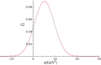
(c) Optimal fit for $s\bar{s}g$.

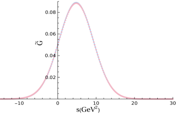
(d) Optimal fit for $u\bar{u}g$.

Figure 8: Next-to-leading order GSR fitting results, dimension-8 condensate is included. Dashed lines mark the optimal value of $s_{0}$, as well as the corresponding $\chi^{2}$ and predicted mass. (c), (d) The optimal fit of $\widetilde{G}_{h}(\tau,s)$ (curves) to $\widetilde{G}(\tau,s,s_{0})$ (dots).

The renormalization-group improved GSR is obtained by setting $\mu^{2}=\sqrt{\tau}$ [gaussian]. We can normalize the $G(\tau,s,s_{0})$ and $G_{h}(\tau,s)$ as:

$$\split\widetilde{G}(\tau,s,s_{0})=&\,\,\frac{G(\tau,s,s_{0})}{\int_{-\infty}^{\infty}ds\,G(\tau,s,s_{0})},\\ \widetilde{G}_{h}(\tau,s)\,\,\,\,=&\,\,\frac{G_{h}(\tau,s)}{\int_{-\infty}^{\infty}ds\,G_{h}(\tau,s)}=\frac{1}{\sqrt{4\pi\tau}}e^{-\frac{(s-m^{2})^{2}}{4\tau}},$$ (15)

where the resonance strength $f$ from eq. 6 has been eliminated, which makes the mass estimation more robust.

It is necessary to keep the width (resolution) of Gaussian kernel finite. A very sharp Gaussian ($\tau\rightarrow 0$) would require knowing the spectral function exactly, which is beyond the current theoretical capacity. A sufficiently wide Gaussian kernel also ensures that a resonance in the spectrum can be approximated by a $\delta$-function. Following Ref. [1--_GSR_chen], we choose $\tau=10\,\text{GeV}^{4}$; the results are not sensitive to the specific choice of $\tau$.

The mass of the lowest-lying resonance can then be estimated by minimizing the $\chi^{2}$:

$$\chi^{2}(\tau,s_{0})=\sum_{i=0}^{N}\big{[}\widetilde{G}(\tau,s_{i},s_{0})-\widetilde{G}_{h}(\tau,s_{i})\big{]}^{2}.$$ (16)

Here,

$$N=\frac{s_{\text}{max}-s_{\text}{min}}{\delta s}+1,\quad s_{i}=s_{\text}{min}+i\,\delta s,$$ (17)

and we choose

$$s_{\text}{min}=-15\text{GeV}^{2},\quad s_{\text}{max}=30\text{GeV}^{2},\quad\delta s=0.2\text{GeV}^{2}.$$ (18)

The $s_{\text}{min}$ and $s_{\text}{max}$ are chosen to be far from the peak of $\widetilde{G}(\tau,s,s_{0})$, while $\delta s$ is chosen to be small enough to capture the detailed structure of $\widetilde{G}(\tau,s,s_{0})$.

To perform a detailed numerical analysis, we vary $s_{0}$ and, for each value, minimize the $\chi^{2}$ with respect to the mass $m$. This yields a minimized $\chi^{2}$ as a function of $s_{0}$, providing a visualization of the solution’s dependence on the continuum threshold $s_{0}$, as presented in figure 8. For $s\bar{s}g$, the optimal choice of $s_{0}$ yields an extremely small $\chi^{2}$. The mass of $u\bar{u}g$ is lower than $s\bar{s}g$ by $\simeq 0.1\text{GeV}$. As summarized in table 2.2, the GSR analysis yields a mass around $2-2.3\,\text{GeV}$, agree with the experimentally measured mass of $\phi(2170)$.

Table 1: GSR fitting results for different scenarios.

wc1.6cmwc1.7cmwc1.7cmwc2.1cmwc2.1cmwc1.7cmwc1.7cm[hvlines]

 

2-1Parameters NLO   NLO, exclude $d=8$ condensate   LO  
$s\bar{s}g$$u\bar{u}g$$s\bar{s}g$$u\bar{u}g$$s\bar{s}g$$u\bar{u}g$
$s_{0}(\text{GeV}^{2})$$5.77\pm 0.08$$5.45\pm 0.90$$6.70\pm 0.27$$6.58\pm 0.27$$9.05\pm 0.45$$8.49\pm 0.35$
$m(\text{GeV})$$2.27\pm 0.01$$2.19\pm 0.14$$2.41\pm 0.04$$2.39\pm 0.04$$2.81\pm 0.05$$2.72\pm 0.04$

 

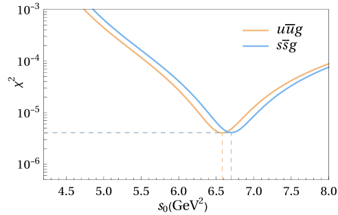
(e) Minimized $\chi^{2}$ versus $s_{0}$.

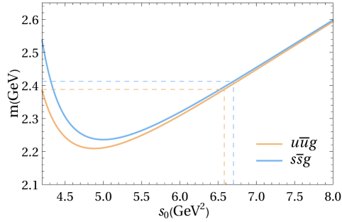
(f) Fitted mass $m$ versus $s_{0}$.

Figure 9: Next-to-leading order GSR fitting results, dimension-8 condensate is excluded. Following the same conventions in figure 8.

2.2.1 Consistency Verification

As a consistency check, we also present the GSR fitting results for the case without including dimension-8 condensate, and the case using LO calculation. As shown in figures 9 and 10. The predicted masses are in excellent agreement with the values derived from the LSR analysis in section 2.1, and the LO GSR fitting result essentially agrees with ref [1--_GSR_chen], despite that dimension-8 condensate is not included there.

Furthermore, the NLO GSR fitting results shows that the optimal continuum thresholds $s_{0}$ determined by the $\chi^{2}$ minimization in the GSR ($s_{0}\approx 5-7\,\text{GeV}^{2}$) are essentially consistent with the $s_{0}$ in LSR where the $\sqrt{\mathcal{R}^{n}}(\tau)$ exhibit stability. Also, despite that the NLO LSR results lack the $\tau$-stability ( figure 5), when we choose the $s_{0}$ corresponding to the table 2.2, and choose $\tau\sim 0.2$ (where $\sqrt{\mathcal{R}^{0}}(\tau)$ is stable, according to figures 4-7), the corresponding masses are $\sim 2.2\text{GeV}$ for $u\bar{u}g$ and $\sim 2.3\text{GeV}$ for $s\bar{s}g$, also agree with the NLO GSR fitting results.

The consistency between these two sum rule methods strengthens the reliability of these mass predictions.

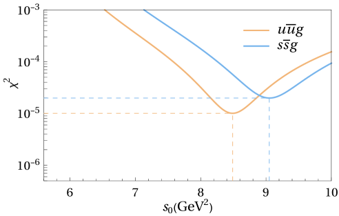
(a) Minimized $\chi^{2}$ versus $s_{0}$.

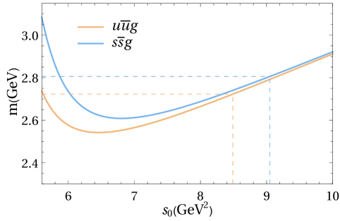
(b) Fitted mass $m$ versus $s_{0}$.

Figure 10: Leading order GSR fitting results. Following the same conventions in figure 8.

3 Conclusion

In a summary, by performing a comprehensive NLO QCD sum rule analysis for the $J^{PC}=1^{--}$ hybrid meson, a conservative mass prediction is in the range of $2-2.5\text{GeV}$ is obtained, and GSR gives preciser mass predictions, with $2.27\pm 0.01\text{GeV}$ for the $s\bar{s}g$ and $2.19\pm 0.14\text{GeV}$ for $u\bar{u}g$. This result is significantly lower than many previous LO sum rule calculations, and reduces the inconsistency between QCD sum rule results and those from lattice QCD ($2.2-2.5\,\text{GeV}$ [1--_lattice_dudek, 1--_lattice_liu]) or the flux-tube model ($2.1-2.2\,\text{GeV}$ [1--_flux_tube]). This demonstrates the importance of NLO corrections in the QCD sum rule analysis of hybrid mesons.

This result also places the predicted mass of the $1^{--}$ hybrid roughly agree with the mass of $\phi(2170)$ resonance, implying that $\phi(2170)$ could be a candidate of $1^{--}$ hybrid, or could contain a large hybrid component if it is a mixed state. To reach a decisive conclusion, further work is required on both the theoretical and experimental sides.

Appendix A Renormalization of Hybrid Current

Figure 11: The diagrams involved in hybrid operator renormalization at $O(g^{2})$.

Consider the generic hybrid operator

$$J=\overline{\Psi}_{f_{a}}g\Gamma G_{\mu\nu}\Psi_{f_{b}},$$ (19)

where $G_{\mu\nu}=T^{n}G^{n}_{\mu\nu}$; $\Gamma$ denotes arbitrary $\gamma$-matrices; $f_{a}$ and $f_{b}$ are flavor indices. For the renormalization at $O(g^{2})$, it is sufficient to consider the Green’s functions:

$$\split\langle T\,J\,&\Psi_{f_{a}}A^{n}_{\alpha}\overline{\Psi}_{f_{b}}\rangle,\\ \langle T\,J\,&\Psi_{f_{a}}\overline{\Psi}_{f_{b}}\rangle,\\ \langle T\,J\,&A^{n}_{\alpha}A^{m}_{\beta}\rangle,\\$$ (20)

where the corresponding diagrams are shown in figure 11. The fermion and gluon fields in eq. 19 are renormalized implicitly, so loops on the external legs need not be considered.

Several observations simplify the determination of the counterterms. The loop integrals in the first, third, fifth, and seventh diagrams in figure 11 are only related to the $G_{\mu\nu}\Psi_{f_{b}}$ part of the operator in eq. 19, as:

$$\vbox{\hbox{ \leavevmode\hbox to1.68pt{\vbox to1.68pt{\text{[drawing]}}}}}\!+\!\vbox{\hbox{ \leavevmode\hbox to1.68pt{\vbox to1.68pt{\text{[drawing]}}}}}\!+\!\vbox{\hbox{ \leavevmode\hbox to1.68pt{\vbox to1.68pt{\text{[drawing]}}}}}\!+\!\vbox{\hbox{ \leavevmode\hbox to1.68pt{\vbox to1.68pt{\text{[drawing]}}}}}=\vbox{\hbox{ \leavevmode\hbox to0pt{\vbox to0pt{\text{[drawing]}}}}}\times\Bigg{\{}\ \ \vbox{\hbox{ \leavevmode\hbox to1.68pt{\vbox to1.68pt{\text{[drawing]}}}}}\!+\!\vbox{\hbox{ \leavevmode\hbox to1.68pt{\vbox to1.68pt{\text{[drawing]}}}}}+\vbox{\hbox{ \leavevmode\hbox to1.68pt{\vbox to1.68pt{\text{[drawing]}}}}}\!+\!\vbox{\hbox{ \leavevmode\hbox to1.68pt{\vbox to1.68pt{\text{[drawing]}}}}}\ \Bigg{\}}.$$ (21)

Therefore, the corresponding counterterm can must be written as:

$$\frac{1}{\varepsilon}\overline{\Psi}\,\Gamma\times\{\text{operatorsactingon}\Psi\}.$$ (22)

Similarly, the loop integral in the ninth diagram in figure 11 only related to $G_{\mu\nu}$, while the loop integrals in the last two diagrams in figure 11 are irrelevant to $G^{n\,\mu\nu}$. In each case, the number of diagrams involved is much smaller than the number of diagrams shown in figure 11. Furthermore, this allows to construct a renormalized hybrid operator for arbitrary $\gamma$-matrices. The result is:

$$\split J_{r}=&\,\,(1+C_{0}+C_{4})Z_{2}^{-1}Z_{3}^{-\frac{1}{2}}\,\overline{\Psi}_{f_{a}}\,g\Gamma G^{\mu\nu}\Psi_{f_{b}}\\ &+C_{1}\,\Big{(}\overline{\Psi}_{f_{a}}\big{[}\big{(}\overleftarrow{\nabla}^{\mu}\overleftarrow{\nabla}^{\rho}+\overleftarrow{\nabla}^{\rho}\overleftarrow{\nabla}^{\mu}\big{)}{\sigma_{\rho}}^{\nu}.\Gamma+\Gamma.{\sigma_{\rho}}^{\nu}\big{(}\nabla^{\mu}\nabla^{\rho}+\nabla^{\rho}\nabla^{\mu}\big{)}\big{]}\Psi_{f_{b}}-\{\mu\leftrightarrow\nu\}\Big{)}\\ &+C_{2}\,\Big{(}\overline{\Psi}_{f_{a}}\big{[}\big{(}\overleftarrow{\not{\nabla}}-i\,m_{f_{a}}\big{)}\gamma^{\nu}.\Gamma gA^{\mu}+gA^{\mu}\Gamma.\gamma^{\nu}.\big{(}\not{\nabla}+i\,m_{f_{b}}\big{)}\big{]}\Psi_{f_{b}}-\{\mu\leftrightarrow\nu\}\Big{)}\\ &+C_{3}\,\overline{\Psi}_{f_{a}}\big{(}\overleftarrow{\nabla}^{2}\sigma^{\mu\nu}.\Gamma+\Gamma.\sigma^{\mu\nu}\nabla^{2}\big{)}\Psi_{f_{b}}\\ &+C_{5}\,\overline{\Psi}_{f_{a}}\big{(}\gamma^{5}.\Gamma+\Gamma.\gamma^{5}\big{)}i\,\varepsilon^{\mu\nu\rho\sigma}G_{\rho\sigma}\Psi_{f_{b}}\\ &+C_{6}\,\Big{(}\overline{\Psi}_{f_{a}}\big{[}-i\sigma^{\mu\rho}.\Gamma+i\Gamma.\sigma^{\mu\rho}\big{]}{G_{\rho}}^{\nu}\Psi_{f_{b}}-\{\mu\leftrightarrow\nu\}\Big{)}\\ &+C_{7}\,\Big{(}\overline{\Psi}_{f_{a}}\big{[}\overleftarrow{\nabla}^{\mu}\gamma^{\nu}.\Gamma m_{f_{a}}+m_{f_{b}}\Gamma.\gamma^{\nu}\nabla^{\mu}\big{]}\Psi_{f_{b}}-\{\mu\leftrightarrow\nu\}\Big{)}\\ &+C_{8}\,\overline{\Psi}_{f_{a}}\big{(}\sigma^{\mu\nu}.\Gamma m_{f_{a}}^{2}+m_{f_{b}}^{2}\Gamma.\sigma^{\mu\nu}\big{)}\Psi_{f_{b}}\\ &+C_{9}\,\overline{\Psi}_{f_{a}}\gamma^{\rho}.\gamma^{\sigma}.\Gamma.\gamma_{\sigma}.\gamma_{\rho}G_{\mu\nu}\Psi_{f_{b}}\\ &+C_{10}\,\delta_{f_{a}f_{b}}\Big{(}\text{Tr}\big{[}\Gamma.\sigma^{\alpha\beta}\big{]}m_{f_{a}}\,G^{n\,\mu\nu}G^{n}_{\alpha\beta}+\frac{2}{3}\text{Tr}\big{[}\Gamma.\gamma_{\alpha}\big{]}G^{n\,\mu\nu}D^{nm}_{\beta}G^{m\,\alpha\beta}\Big{)}.$$ (23)

Here, the fields on the right-hand side are bare fields; the

$$Z_{2}=1-\frac{g^{2}C_{F}}{16\pi^{2}\varepsilon}\quad\text{and}\quad Z_{3}=1-\frac{g^{2}}{16\pi^{2}\varepsilon}\Big{[}-\frac{5}{3}C_{A}+\frac{2}{3}n_{f}\Big{]}$$ (24)

are fermion and gluon renormalization constants in Feynman gauge. The values of $C_{n}$ in Feynman gauge are listed in table 2. Massive quark propagators are used to obtain these values; $C_{8}$ vanishes in the $m^{2}\rightarrow 0$ limit. Note that the term $\propto C_{2}$ is not gauge invariant, but it is vanished under equation of motion, as the non-gauge-invariant counterterms should be [book_ren]. The $C_{0}$ corresponds to the third to last diagram in figure 11, while the $C_{9}$ and $C_{10}$ correspond to the last two diagrams. We do not combine the $C_{0}$ and $C_{4}$ into a single constant, because the $C_{0}$ directly related to the cancellation of IR-pole, as we discussed around eq LABEL:IR_cancel. For the $\langle GG\rangle$ diagrams shown in figure 2, the renormalized coupling constant $g$ should be written explicitly as

$$g=Z_{g}^{-1}g_{0}=\big{[}1+\frac{g^{2}}{16\pi^{2}\varepsilon}\big{(}\frac{11}{6}C_{A}-\frac{1}{3}n_{f}\big{)}\big{]}g_{0},$$ (25)

to ensure the cancellation of $\log/\varepsilon$-pole and the $n_{f}$-dependence in $Z_{3}$, since no $n_{f}$-dependent diagram involved in the $\langle GG\rangle$ diagrams.

Table 2: The coefficients of each counterterm in eq. 23, obtained under Feynman gauge, and $d=4-2\varepsilon$.

0pt   $C_{0}$ $C_{1}$ $C_{2}$ $C_{3}$ $C_{4}$ $C_{5}$   $\frac{3C_{A}g}{32\pi^{2}\varepsilon}$ $\frac{C_{F}g^{2}}{192\pi^{2}\varepsilon}$ $\frac{C_{A}g^{2}}{128\pi^{2}\varepsilon}$ $\frac{C_{F}g^{2}}{96\pi^{2}\varepsilon}$ $-\frac{C_{A}g}{16\pi^{2}\varepsilon}$ $\frac{C_{A}g^{2}}{128\pi^{2}\varepsilon}$   $C_{6}$ $C_{7}$ $C_{8}$ $C_{9}$ $C_{10}$   $\frac{(3C_{A}^{2}+1)g^{2}}{128C_{A}\pi^{2}\varepsilon}$ $\frac{C_{F}g^{2}}{32\pi^{2}\varepsilon}$ $\frac{C_{F}g^{2}}{32\pi^{2}\varepsilon}$ $\frac{g^{2}}{128C_{A}\pi^{2}\varepsilon}$ $\frac{g^{2}}{64\pi^{2}\varepsilon}$   UlFFS

Appendix B OPE Diagrams and Relevant Technical Details

The calculation of the OPE involves numerous diagrams. The relevant diagrams and necessary technical details are presented here. Except the NLO diagrams shown in figures 1-3, the LO diagrams are shown here (figures 12-14). The equations used to evaluate the dimension-6 condensates are listed in eqs 12-27. Note the $\langle GGG\rangle$ diagrams do not contribute to imaginary part of the correlator. The evaluation of $\langle GG\rangle$ diagrams involves infrared divergence, the cancellation infrared divergence is discussed in section B.1. The evaluation of dimension-8 four-quark condensate is discussed in section LABEL:d8_factor.

(a) $m\langle\bar{q}q\rangle$.

(b) $\langle GGG\rangle$.

Figure 12: Diagrams corresponding to $m\langle\bar{q}q\rangle$ and $\langle GGG\rangle$, Eq. 27 is used to obtain $\langle GGG\rangle$.

Figure 13: Diagrams corresponding to $\langle qq\rangle^{2}$ and $m\langle qGq\rangle$. The terms like $\langle\bar{q}^{a}_{i}G_{\alpha\beta}\nabla_{\nu}q^{b}_{j}\rangle$ and $\langle\bar{q}^{a}_{i}D_{\alpha}G^{n}_{\beta\mu}q^{b}_{j}\rangle$ can be written to $\langle qq\rangle^{2}$ and $m\langle qGq\rangle$ by Eq. 26.

Figure 14: Diagrams corresponding to $\langle\bar{q}q\rangle\langle\bar{q}Gq\rangle$.

To obtain the $\langle qq\rangle^{2}$ and $m\langle qGq\rangle$ contributions from figure 13, the following identities are used [high_order_condensates]:

$$\split\langle\bar{q}_{i}^{a}\nabla_{\alpha}\nabla_{\beta}\nabla_{\nu}q_{j}^{b}\rangle=\frac{i\delta^{ab}}{C_{A}}\times\bigg{[}&\frac{C_{F}\,g^{2}}{32C_{A}(d-1)}\langle\bar{q}q\rangle^{2}\Big{(}\frac{-g_{\alpha\beta}\gamma_{\nu}+(d+1)g_{\alpha\nu}\gamma_{\beta}-g_{\beta\nu}\gamma_{\alpha}}{d+2}-\frac{\gamma_{\alpha\beta\nu}}{d-2}\Big{)}\\ &-m\langle\bar{q}Gq\rangle\Big{(}\frac{g_{\alpha\beta}\gamma_{\nu}+g_{\alpha\nu}\gamma_{\beta}+g_{\beta\nu}\gamma_{\alpha}}{8d(d+2)}+\frac{\gamma_{\alpha\beta\nu}}{8d(d-1)(d-2)}\Big{)}\\ &-m^{3}\langle\bar{q}q\rangle\frac{\gamma_{\alpha\beta\nu}}{4d(d-1)(d-2)}\bigg{]}_{ji},$$ (26)

$$\split\langle g^{2}G^{n}_{\mu\nu}D_{\alpha}D_{\beta}G^{m}_{\rho\sigma}\rangle=&\frac{\delta^{nm}}{C_{A}C_{F}d(d-1)(d^{2}-4)}\times\\ &\big{[}-(d+2)\langle O^{6}_{1}\rangle(\!(\!(g_{\sigma\mu}g_{\nu\alpha}g_{\beta\rho}\!-\!(\mu\leftrightarrow\nu))\!-\!(\rho\leftrightarrow\sigma))\!-\!(\alpha\leftrightarrow\beta))\\ &\quad+\big{[}(d-4)\langle O^{6}_{1}\rangle+(d-2)\langle O^{6}_{2}\rangle\big{]}\\ &\qquad\times(((g_{\sigma\mu}g_{\nu\alpha}g_{\beta\rho}-(\mu\leftrightarrow\nu))-(\rho\leftrightarrow\sigma))+(\alpha\leftrightarrow\beta))\\ &\quad-\big{[}4(d-1)\langle O^{6}_{1}\rangle+2(d-2)\langle O^{6}_{2}\rangle\big{]}g_{\alpha\beta}(g_{\mu\rho}g_{\nu\sigma}-(\rho\leftrightarrow\sigma))\big{]}.$$ (27)

Here, vacuum saturation hypothesis is adopted for $\langle\bar{q}q\rangle^{2}$, and

$$\split\langle O^{6}_{1}\rangle=&-\frac{1}{4}\langle g^{3}f^{abc}G^{a}_{\eta\mu}G^{b}_{\mu\nu}G^{c}_{\nu\eta}\rangle,\\ \qquad\langle O^{6}_{2}\rangle=&-\frac{dC_{F}}{8C_{A}}g^{2}\sum_{q}\langle\bar{q}q\rangle^{2},$$ (28)

where $\sum_{q}$ means sum over the flavors.

B.1 Gluon Propagators and Cancellation of IR Pole

Following a procedure similar to that in Ref [high_order_condensates], the gluon propagator in the background gluon field can be derived as follows. Written gluon field as $a_{\mu}^{n}+A_{\mu}^{n}$, where $a_{\mu}$ is quantum gluon field and $A_{\mu}$ is background gluon field. By choosing gauge-fixing term as $-\frac{1}{2}(\partial_{\mu}a_{\nu})^{2}$, the required gluon vertices are [1-+_jin]:

$$\split\leavevmode\hbox to63.04pt{\vbox to23.08pt{\text{[drawing]}}}&=iG_{\alpha\beta}+(q^{\rho}A_{\rho}+A_{\rho}q^{\rho})g_{\alpha\beta}-(q_{\beta}A_{\alpha}+A_{\beta}q_{\alpha}),\\ \leavevmode\hbox to63.04pt{\vbox to23.08pt{\text{[drawing]}}}&=ig^{2}f^{anc}f^{cmb}A^{n\,\rho}A^{m}_{\rho}g_{\alpha\beta}-ig^{2}f^{anc}f^{cmb}A^{m}_{\alpha}A^{n}_{\beta}, {}^{a}_{\alpha} \,\,{}^{b}_{\beta} x \leftarrow q {}^{a}_{\alpha} \,\,{}^{b}_{\beta} x \leftarrow q$$ (29)

where we adopt the matrix notations $G_{\mu\nu}=gf^{anb}G^{n}_{\mu\nu}(x)$ and $A_{\mu}=gf^{anb}A^{n}_{\mu}(x)$. The ordering of background gluon field $A$ and momentum $q$ is important, as

$$A^{n}_{\mu}(x)=\frac{1}{2}x^{\rho}G^{n}_{\rho\mu}(0)+\frac{1}{3\cdot 1!}x^{\rho}x^{\eta}D_{\rho}G^{n}_{\eta\mu}(0)\cdots$$ (30)

in Fock-Schwinger gauge [high_order_condensates], and $x$ can be written to $-i\partial_{q}$ or $i\overleftarrow{\partial_{q}}$ in propagator.

Alternatively, choosing the commonly adopted gauge fixing term $-\frac{1}{2}(D_{\mu}a_{\nu})^{2}$ in QCD sum rules [high_order_condensates], where $D_{\mu}=\partial_{\mu}+gf^{anb}A_{\mu}^{n}$, the gluon vertices becomes:

$$aαbβx←q$$ (31)