Over the Stability Space of a Multivariate Time Series

Abstract

This paper jointly addresses the challenges of non-stationarity and high dimensionality in analysing multivariate time series. Building on the classical concept of cointegration, we introduce a more flexible notion, called stability space, aimed at capturing stationary components in settings where traditional assumptions may not hold. Based on the dimensionality reduction techniques of Partial Least Squares and Principal Component Analysis, we proposed two non-parametric procedures for estimating such a space and a targeted selection of components that prioritises stationarity. We compare these alternatives with the parametric Johansen procedure, when possible. Through simulations and real-data applications, we evaluated the performance of these methodologies across various scenarios, including high-dimensional configurations.

[1]organization=STOR-i Centre for Doctoral Training, Lancaster University, addressline=Science & Technology Building, city=Lancaster, postcode=LA1 4YR, country=United Kingdom

[2]organization=Institute of Data Science and Artificial Intelligence, University of Navarra, addressline=Campus Universitario, city=Pamplona, postcode=31009, country=Spain

[3]organization=School of Economics & Business, University of Navarra, addressline=Campus Universitario, city=Pamplona, postcode=31009, country=Spain

[4]organization=National Institute of Statistics and Geography (INEGI), addressline=Av. Patriotismo 711, city=Mexico City, postcode=03730, country=Mexico

Declaration of interests

The authors declare that they have no known competing financial interests or personal relationships that could have appeared to influence the work reported in this paper.

1 Introduction

The study of phenomena or processes exhibiting temporal dependence arises naturally in various fields such as economics, environmental sciences, and epidemiology, for example, in the analysis of Gross Domestic Product per capita (James et al., 2012), global surface temperature (Kaufmann et al., 2006), or daily mortality rates (Bhaskaran et al., 2013). Although statistical methods serve various purposes in this context, many rely –at least to some extent– on the assumption that the underlying stochastic process is stationary in order to establish theoretical and practical properties. This is particularly true in time series analysis.

Let $\{X_{n},n\in\mathbb{Z}\}$ denote a time series in $\mathbb{R}^{m}$. Generally, each of the $m$ components of the series $X$ corresponds to a variable, and these variables interact with one another. Let $\{X_{n},n=1,\dots,T\}$ represent a random sample from the series $\{X_{n},n\in\mathbb{Z}\}$. To illustrate the importance of the stationarity assumption, consider the $h$-step-ahead forecasting problem: inferring the distribution of the variables $X_{T+1},\dots,X_{T+h}$ based on the observed data. It is well-known that both Dynamic Factor Models and Vector Autoregressive (VAR) models rely on the assumption of stationarity for forecasting purposes; see Stock and Watson (2002) and Lütkepohl (2005), respectively. Under the stationarity assumption and employing a VAR model, it is possible to derive the asymptotic distribution of these variables, thereby enabling the construction of both point forecasts and prediction intervals. Similarly, certain time series clustering algorithms (Maharaj, 2000) and changepoint detection methods (Killick et al., 2012) also presuppose stationarity.

In the absence of stationarity, a different approach is required. In fact, numerous real-world applications involve non-stationary features, as illustrated by analysis of business cycles (Hamilton, 1989), as well as studies in biomedical signal processing and seismology (Adak, 1998). Non-stationarity may arise for various reasons, including deterministic trends, structural changes, seasonal behaviours, or unit roots. In this work, we address non-stationarity arising from unit roots or stochastic trends. The concepts and techniques introduced in this work offer a different approach to this longstanding problem, leveraging dimensionality reduction techniques.

Another key aspect of modern data analysis is the prevalence of phenomena involving many interacting variables. In the time series context, this gives rise to the challenge of modelling high-dimensional multivariate time series. High dimensionality typically refers to situations where the number of variables or series, $m$, is on the order of hundreds or thousands, and often substantially exceeds the length of the series, $T$. For example, Peña et al. (2019) discusses practical cases in which $m$ is ten times greater than $T$. Moreover, when $m\gg 0$, various estimation challenges emerge. In VAR models, for instance, multicollinearity and parameter instability naturally arise. Consequently, it is of practical interest to represent and decompose the information using a smaller number of uncorrelated latent variables –in other words, to perform dimensionality reduction. A comprehensive summary of this approach in the time series context is provided by Lam et al. (2011). The techniques introduced therein enable analysis in high-dimensional settings.

To tackle the simultaneous challenges of non-stationarity and high dimensionality, we introduce a methodology building upon the concept of cointegration, as originally formulated by Engle and Granger (1987). In this regard, the methodology for analysing cointegration in multivariate time series proposed by Johansen (1991) is particularly influential, as it allows the estimation of a basis for the so-called cointegration space. However, one of the main limitations of Johansen’s procedure is that it becomes computationally infeasible in high-dimensional systems. Moreover, it is a parametric approach that relies on a set of formal assumptions which may not be plausible in practice. This motivates the introduction of a new concept, referred to as the stability space, which we will discuss throughout this work.

There are alternative approaches to Johansen’s method that also target the cointegration context and offer certain advantages, as they are based on non-parametric dimensionality reduction techniques. In this article, we examine the approaches of Muriel et al. (2012), based on the Partial Least Squares (PLS) algorithm (Wold, 1966), and Harris (1997), based on Principal Component Analysis (PCA) (Hotelling, 1933). These methods provide a useful starting point, as they have inspired a wide range of interesting extensions and modifications in the literature. Moreover, we argue that the greater flexibility of these approaches may be advantageous for estimating the less restrictive concept of stability space, which, for example, allows the construction of forecasts that are well-behaved in the long run.

After applying a dimensionality reduction method, one typically obtains a smaller number of components with which to optimally represent the original information according to some criterion. For example, in PCA, it is common to retain the first two principal components. However, these first two principal components are not guaranteed to yield stationary time series –in fact, as we shall demonstrate in this article, one should often expect the opposite. We therefore propose selecting the first principal components that produce stationary time series, which is more appropriate, given that time series methods are typically applied to these latent variables.

This article is organised as follows: Section 2 discusses the concept of cointegration and how it motivates the introduction of the stability space, which is addressed in Section 3. Section 4 describes the most relevant aspects of the methodologies considered: Johansen’s approach and those based on PLS and PCA. Section 5 presents the theoretical aspects of a novel simulation study designed to evaluate these methodologies and the results of this assessment. This simulation procedure is itself of independent interest, as it enables the generation of time series with a specified cointegration space –or, more accurately, with a given stability space. Finally, in Section 6 we apply the discussed methodologies in economics practical examples, considering both low- and high-dimensional cases. The paper ends with a discussion in Section 7. The mathematical proofs and the code associated with this work are in the Appendix.

2 Cointegration notion

Consider a time series $\{X_{n},n\in\mathbb{Z}\}$ taking values in $\mathbb{R}^{m}$, such that $\mathbb{E}[\lVert X_{n}\rVert^{2}]<\infty$.

Definition 2.1

The difference operator $\Delta$ is defined as

$$\Delta X_{n}:=X_{n}-X_{n-1}\quad\text{for all }n\in\mathbb{Z}.$$

The series $\{X_{n},n\in\mathbb{Z}\}$ is said to be integrated of order $d\in\mathbb{N}$ if $d$ is the smallest natural number such that the series $\{\Delta^{d}X_{n},n\in\mathbb{Z}\}$ is stationary. We denote this property as $X\sim\textsf{I}(d)$. Here, $\Delta^{d}$ denotes the application of the difference operator $d$ times.

The cases $d=0$ and $d=1$ (a unit root) are commonly considered. In the case $d=0$, the process is stationary, whereas for $d=1$, the process variance diverges, and innovations have a permanent effect on the process.

However, when considering the notion of equilibrium among the variables of a multivariate time series, it is possible to combine these non-stationary behaviours to obtain a stationary process. This is precisely the idea of cointegration among time series, a concept rigorously formalised in Engle and Granger (1987).

Definition 2.2

Consider

$$X_{n}=[X_{1,n},\dots,X_{m,n}]^{\prime}\quad\text{for all }n\in\mathbb{Z},$$

where $X_{i,n}$ is the $i$-th coordinate of the vector $X_{n}$.

Let $\tilde{X}_{i}:=\{X_{i,n},n\in\mathbb{Z}\}$ denote the univariate time series corresponding to the $i$-th coordinate of the process $\{X_{n},n\in\mathbb{Z}\}$.

The series $\tilde{X}_{1},\dots,\tilde{X}_{m}$ are said to be cointegrated of order $\textsf{CI}(d,b)$, denoted $X\sim\textsf{CI}(d,b)$, if:

1. $\tilde{X}_{i}\sim\textsf{I}(d)$ for all $i=1,\dots,m$;

2. There exists $\beta\in\mathbb{R}^{m}$, with $\beta\neq 0$, such that $\{Z_{n}:=\beta^{\prime}X_{n},n\in\mathbb{Z}\}\sim\textsf{I}(d-b).$ The vector $\beta$ is referred to as a cointegration vector or relation.

Under the above definition, cointegration relations are not necessarily unique. If there exist at most $r$ linearly independent cointegration vectors, then $r$ is referred to as the cointegration rank. The vector space spanned by these $r$ vectors is known as the cointegration space.

In the particular case $X\sim\textsf{CI}(1,1)$, if $\beta$ is a cointegration relation, then $Z$ is a stationary process. In general, cointegration relations are those that reduce the order of integration of the series involved.

On the other hand, by the Wold Decomposition Theorem, any stationary process $X$ can be expressed as the sum of two uncorrelated processes, $\{V_{n},n\in\mathbb{Z}\}$ and $\{U_{n},n\in\mathbb{Z}\}$, as follows:

$$X_{n}=V_{n}+U_{n}\quad\text{for all }n\in\mathbb{Z},$$

where $V$ is a deterministic process fully determined by its past, and $U$ is a purely non-deterministic process satisfying $\mathbb{E}[U_{n}]=0$ for all $n$. In what follows, we refer to $U$ as the stochastic component of the process $X$.

We now introduce several important assumptions that will allow us to analyse different scenarios regarding the sources of non-stationarity. These assumptions are necessary for certain results in the analysis of cointegration. However, as will be discussed later, they may be flexibilized when applying the methodologies presented in Harris (1997); Muriel et al. (2012).

Assumption 1

By the discussion above, although $X$ may be non-stationary, we focus on series without deterministic components. Specifically, we assume that $X$ is a non-stationary stochastic process with zero mean, i.e., a mean-return process.

In practice, such deterministic components can be removed, for example, by using the residuals from a regression of the form:

$$X_{n}=a+bn+U_{n}.$$

This regression assumes that the deterministic component is linear. The validity of this assumption is discussed in Section 15.2 of Hamilton (2020). Alternative approaches can also be considered, depending on the particular problem under study. Moreover, we also assume that the underlying series does not contain seasonal components.

Under Assumption 1, the series $X$ may be considered to have the initial condition $X_{0}=0$, i.e., $X_{n}=0$ almost surely for $n\leq 0$.

The scenario that defines the cointegration context for subsequent analysis is summarised in the following assumption:

Assumption 2

We consider Assumption 1, and additionally that $X$ follows a VAR model of order $p$ and satisfies $X\sim\textsf{CI}(1,1)$, with cointegration rank $r$.

A key result presented in Engle and Granger (1987), which links series satisfying Assumption 2 to VECM models (Sargan, 1964; Davidson et al., 1978), is the Granger Representation Theorem (Engle and Granger, 1987). We state below the version presented in Lütkepohl (2005):

Theorem 2.1

Let $X\sim\text{VAR}(p)$ such that $X\sim\textsf{CI}(1,1)$ and is a purely non-deterministic process.

Suppose it has a VECM representation:

$$\Delta X_{n}:=\alpha\beta^{\prime}X_{n-1}+\sum_{j=1}^{p-1}\Gamma_{j}\Delta X_{n-j}+\epsilon_{n},$$ (1)

with $X_{n}=0$ for $n<0$, and where $\epsilon$ is white noise with $\epsilon_{n}=0$ for $n\leq 0$.

Consider the polynomial

$$C(z):=(1-z)I_{m}-\alpha\beta^{\prime}z-\sum_{j=1}^{p-1}\Gamma_{j}(1-z)z^{j}.$$

Suppose the following conditions hold:

1. If $\det C(z)=0$, then $|z|\geq 1$.

2. The number of unit roots is $m-r$.

3. $\alpha,\beta\in\mathbb{R}^{m\times r}$, with $\operatorname{rank}(\alpha)=\operatorname{rank}(\beta)=r$.

Then,

$$X_{n}=\mathfrak{F}\sum_{i=1}^{n}\epsilon_{i}+\mathfrak{F}^{\star}(L)\epsilon_{n}+X_{0}^{\star},$$

where

$$\mathfrak{F}=\beta_{\perp}\left[\alpha_{\perp}^{\prime}\left(I_{m}-\sum_{i=1}^{p-1}\Gamma_{i}\right)\beta_{\perp}\right]^{-1}\alpha_{\perp}^{\prime}.$$

It follows that $\operatorname{rank}(\mathfrak{F})=m-r$, $\mathfrak{F}^{\star}(L)\epsilon_{n}:=\sum_{j=0}^{\infty}\mathfrak{F}^{\star}_{j}\epsilon_{n-j}\sim\textsf{I}(0)$, and that $\beta_{\perp},\alpha_{\perp}\in\mathbb{R}^{m\times(m-r)}$ are matrices whose columns are orthogonal to the columns of $\beta$ and $\alpha$, respectively.

From this result, the following proposition can be derived.

Proposition 2.2

Let $\{X_{n},n\in\mathbb{Z}\}$ be a time series in $\mathbb{R}^{m}$ satisfying Assumption 2. The following decomposition holds:

$$X_{n}=P_{\beta_{\perp}}\left(\theta(1)\sum_{i=1}^{n}\epsilon_{i}\right)+P_{\beta}X_{n}+\eta_{n}\quad\text{for all }n\geq 0,$$ (2)

where $P_{\beta},P_{\beta_{\perp}}$ are projection matrices onto the column spaces $\operatorname{Col}(\beta)$ and $\operatorname{Col}(\beta_{\perp})$, respectively, $\{\eta_{n},n\in\mathbb{Z}\}$ is a stationary time series, and:

$$Z_{n}:=P_{\beta}X_{n}+P_{\beta_{\perp}}\Delta X_{n},$$

has a moving average (MA) representation

$$Z_{n}=\theta(B)\epsilon_{n}.$$

Thus, the series $\{P_{\beta}X_{n},n\in\mathbb{Z}\}$ represents the stationary component of the series $\{X_{n},n\in\mathbb{Z}\}$.

3 Stability Space

Proposition 2.2 motivates the idea of considering a vector space onto which the projection of the time series under study is stationary. In principle, under Assumption 2, this vector space coincides with the cointegration space. However, without this restriction, such a space may still exist, but it would no longer correspond to the cointegration space, representing instead a different notion.

Firstly, Assumption 1, despite allowing for a non-stationary process, attempts to simplify the problem by considering this non-stationarity to arise solely from a time series without a determinist component. Assumption 2 is more restrictive and is not valid, for instance, for a series $\{X_{n},n\in\mathbb{Z}\}$ whose components exhibit different orders of integration.

Thus, the notion of a vector $\bm{v}\in\mathbb{R}^{m}$ such that the series $\{\bm{v}^{\prime}X_{n},n\geq 0\}$ is stationary is not subject to either Assumption 1 or Assumption 2, which motivates the following definition.

Definition 3.1

Let $\{X_{n},n\geq 0\}$ be a time series in $\mathbb{R}^{m}$. We say that $\bm{v}\in\mathbb{R}^{m}$ is a stability relation if the time series $\{\bm{v}^{\prime}X_{n},n\geq 0\}$ is stationary.

Moreover, we define the stable space as

$$\mathcal{H}^{S}:=\{\bm{v}\in\mathbb{R}^{m}\ |\ \bm{v}\text{ is a stability relation}\}.$$

The space $\mathcal{H}^{N}:=(\mathcal{H}^{S})^{\perp}$ is referred to as the instability space.

Remark 1

Under Assumption 2, the subspace $\mathcal{H}^{S}$ coincides with the cointegration space. Using the notation of Proposition 2.2, we have $\mathcal{H}^{S}=\text{Col }\beta$.

Remark 2

The notion of the stable space could be applied to a time series without distinguishing the underlying cause of its non-stationarity (unit root, structural break, deterministic trend, fractional order of integration), although this idea would require further formalisation.

Therefore, unlike Johansen’s procedure, which heavily depends on Assumption 2, this is not the case for the methodologies proposed in Muriel et al. (2012) and Harris (1997). In fact, Wold (1980) notes that the PLS algorithm can be used in complex variable systems with few theoretical assumptions. Thus, these methodologies can be employed to identify a basis for the stable space $\mathcal{H}^{S}$.

Assuming $\dim\mathcal{H}^{S}=r$, each of these methodologies yields an estimated matrix $\hat{\beta}=[\hat{\beta}_{1},\dots,\hat{\beta}_{\hat{r}}]$, whose columns form an estimated basis of the stable space $\mathcal{H}^{S}$. Here, $\text{Col }\hat{\beta}$ denotes the estimated space, and $\hat{r}$ is the estimated dimension, which may vary across methods. In principle, $\hat{\beta}$ differs from one method to another, although the vector space $\text{Col }\hat{\beta}$ may coincide. Further details on the estimation procedure are provided in Section 4.

The column vectors $\hat{\beta}_{i}$, for $i=1,\dots,\hat{r}$, will represent the estimated stable components of the time series $X$, and

$$T_{i}(n):=\hat{\beta}_{i}^{\prime}X_{n}\quad\text{ for }n\geq 0,$$

the stationary scores associated with these components.

The stationary scores represent the relationships among the variables comprising the time series. For example, let $\hat{\beta}_{1}=[\hat{\beta}_{1,1},\dots,\hat{\beta}_{1,m}]^{\prime}$, then, the weights $\hat{\beta}_{1,j}$ indicate the extent and manner in which the variable $X_{j,n}$ contributes to the score $T_{1}(n)$. In this way, this concept allows one to obtain stationary latent variables from a vector time series by combining information from its constituent series. Thus, these scores reveal how the series within the system compensate each other to achieve long-term stability.

4 Methodology

We shall now describe the various methodologies that will be considered for estimating the columns of $\beta=[\beta_{1},\dots,\beta_{r}]$, which will correspond to the estimated basis of the stable space $\mathcal{H}^{S}$. All methodologies begin with a random sample $\{X_{n},n=1,\dots,T\}$ from a time series taking values in $\mathbb{R}^{m}$.

4.1 Johansen Procedure

One of the most widely used methods for estimating the cointegration space is the Johansen procedure, introduced in Johansen (1991). This methodology relies heavily on Assumption 2 and is based on the VECM parametrisation of $X$ in (1).

We now summarise the steps that constitute the Johansen procedure. Let

$$M_{p-1}(n):=\textsc{span}\{\Delta X_{n-1},\dots,\Delta X_{n-p+1}\}$$

Using the Projection Theorem, we can obtain the decompositions

$$\Delta X_{n}=R_{0n}+P_{M_{p-1}(n)}\Delta X_{n}\in\mathbb{R}^{m},$$

and

$$X_{n-1}=R_{1n}+P_{M_{p-1}(n)}X_{n-1}\in\mathbb{R}^{m},$$

where $R_{0n}=P_{M_{p-1}(n)^{\perp}}\Delta X_{n}$ and $R_{1n}=P_{M_{p-1}(n)^{\perp}}X_{n-1}$.

Therefore, by applying $P_{M_{p-1}(n)^{\perp}}$ to (1), we obtain the relation

$$R_{0n}=\alpha\beta^{\prime}R_{1n}+\epsilon_{n},$$

with $\{\epsilon_{n},n=1,\dots,T\}$ being centred Gaussian noise.

The Johansen procedure estimates $\alpha$ and $\beta$ from the above relation using maximum likelihood, since Gaussian noise is assumed.

The main interest lies in estimating $\beta$. In Maddala and Kim (1998), it is shown that, under normality and assuming the cointegration rank $r$ is known, the maximum likelihood estimator of $\beta$ is equivalent to the matrix whose columns correspond to the first $r$ asymptotic canonical correlations between $R_{0n}$ and $R_{1n}$.

This is due to the fact that we attempt to linearly predict an $\textsf{I}(0)$ process ($\Delta X_{n}$) with an $\textsf{I}(1)$ process ($X_{n-1}$), and thus, intuitively, we seek the linear combinations of $X_{n-1}$ that are most correlated with $\Delta X_{n}$.

To obtain an estimator $\hat{r}$ of $r$, Johansen (1991) proposes a method based on the likelihood ratio test. This is described in Section 6.5.1 of Maddala and Kim (1998). In summary, the estimator $\hat{r}$ is obtained by successively applying the likelihood ratio test

$$H_{0}:r\leq r_{0}\quad\text{vs}\quad H_{a}:r>r_{0},$$

whose test statistic is

$$\Lambda_{r_{0}}:=-T\sum_{i=r_{0}+1}^{m}\log(1-\hat{\lambda}_{i}),$$

where $\hat{\lambda}_{i}$ corresponds to the $i$-th estimated canonical correlation.

When, for the first time, there is no evidence to reject the null hypothesis as the value of $r_{0}$ increases, an estimator is obtained—in this case, of the cointegration rank, that is, $\hat{r}=r_{0}$.

We note that the Johansen procedure is based on the following assumptions:

1. Assumption 2.

2. A Gaussian innovation process for the underlying process $X$. The Johansen procedure is sensitive to this assumption, as illustrated in Gonzalo and Lee (1998); Huang and Yang (1996).

Moreover, Maddala and Kim (1998) indicates that critical values for this hypothesis test can be found in Osterwald-Lenum (1992) for processes with $m\leq 11$. Precisely because of this, implementations of this method, such as the ca.jo class from the urca R package (Pfaff, 2008), only support systems with $m\leq 11$.

Theoretically, it is possible to carry out the Johansen procedure for any value of $m$, however, it becomes computationally prohibitive. For this reason, the methodology is limited in the context of high dimensionality. Thus, the parametric nature of this methodology, Assumption 2, and the issue of high dimensionality are all constraints that limit the practical applicability of the Johansen procedure.

4.2 PCA

A first alternative for the estimation of $\beta$ is the approach proposed in Harris (1997). In Harris (1997), the estimation of $\beta$ is carried out under Assumption 2; however, we propose to apply the same methodology while relaxing these assumptions.

The main motivation lies in the intuition behind the Johansen procedure, which seeks to linearly predict $\Delta X_{n}$ using $X_{n-1}$. In order to avoid differencing the series and to perform the analysis at the level of the original series, the core idea of the methodology proposed by Harris (1997) is to analyse the variability of the original series $\{X_{n},n=1,\dots,T\}$.

For example, under Assumption 2, $X_{n}$ has components that are at least $\textsf{I}(1)$, and we aim to predict $X_{n}$ by identifying linear combinations of its components that yield a stationary time series. These linear combinations are expected to exhibit lower variability, as they correspond to an $\textsf{I}(0)$ process. Consequently, PCA is based on the notion that the stable linear combinations of a process with non-stationary components should correspond to the principal components with the lowest variability.

Therefore, if $r$ is known, an estimator for the columns of $\beta$ is the matrix formed by the $r$ eigenvectors associated with the $r$ smallest eigenvalues from the spectral decomposition of the sample covariance matrix

$$S:=T^{-1}\sum_{i=1}^{T}X_{i}X_{i}^{\prime}.$$

In the steps of this methodology, Assumption 2 is not theoretically essential, unlike in the Johansen procedure, although it is necessary for deriving the asymptotic properties of the obtained estimator, as detailed in Harris (1997).

Thus, to estimate $\beta$ and the dimension $r$ of the stable space $\mathcal{H}^{S}$, one first computes the eigenvectors $\hat{\beta}_{1},\dots,\hat{\beta}_{m}$ associated with the eigenvalues

$$\hat{\lambda}_{1}\geq\dots\geq\hat{\lambda}_{m},$$

of $S$. Subsequently, we consider

$$T_{i}(n)=\hat{\beta}_{i}^{\prime}X_{n}\quad\text{ for }n=1,\dots,T,$$

and the hypothesis test

$$H_{0}:\ r\geq r_{0}\quad\text{vs}\quad H_{a}:\ r<r_{0}.$$ (3)

Moreover, as noted in Harris (1997), it is observed that for $i<j$, if the series $\{T_{i}(n),n=1,\dots,T\}$ is stationary, then $\{T_{j}(n),n=1,\dots,T\}$ is also stationary.

Therefore, the hypothesis test in (3) is equivalent to

$$H_{0}:\ T_{m-r_{0}+1}\sim\textsf{I}(0)\quad\text{vs}\quad H_{a}:\ T_{m-r_{0}+1}\sim\textsf{I}(1),$$

and this test can be carried out, for example, using the KPSS test (Kwiatkowski et al., 1992), while, if the null and alternative hypotheses are switched, the augmented Dickey–Fuller (ADF)(Dickey et al., 1986) test may be used. However, it is more convenient to consider stationarity in the null hypothesis—first, because we are logically seeking statistical evidence to rule out non-stationary scores, and second, because it avoids the issue that arises from the presence of multiple unit roots when using the ADF test setup, as discussed in (Dickey and Pantula, 1987). Indeed, the recommended scenario outside the scope of Assumption 2 is to consider different higher orders of integration, as will be detailed in Section 5.

Although $\hat{r}$ is the first value of $r_{0}$ for which the null hypothesis of the previous test is not rejected—under Assumption 2—we consider relaxing this assumption. Consequently, we take as the estimator of $\beta$ the components that give rise to stationary scores, that is,

$$\hat{\beta}_{\textsc{PCA}}:=[\hat{\beta}_{i},\dots,\hat{\beta}_{i_{\hat{r}}}],$$

where $\hat{\beta}_{i_{k}}$ for $k=1,\dots,\hat{r}$ denotes the set of components, which are not necessarily consecutive but are ordered by importance with respect to the spectral decomposition, such that $T_{i_{k}}$ is not rejected as being a stationary series. The subscript indicates the method used for the estimation.

We observe that this PCA-based method relies on the decomposition of the variance of the process $X$, rather than on the dependence between the variables $X_{n}$ and $X_{n-1}$, which naturally arises in a time series. This aligns with the intuition behind the following methodology.

4.3 PLS

It is of interest to analyse the covariance between the variables $X_{n}$ and $X_{n-1}$—which is ignored by the PCA-based methodology but is considered in the Johansen procedure, although the latter does so between $\Delta X_{n}$ and $X_{n-1}$. Moreover, obtaining stationary scores leads to identifying the directions $\hat{w}_{i}$ with the lowest variability, as in Harris (1997). These are the main motivations for the methodology proposed in Muriel et al. (2012).

In Muriel et al. (2012), a PLS procedure is proposed to estimate cointegrating vectors, assuming that

$$\mathbf{Y}:=[X^{\prime}_{T},\dots,X^{\prime}_{2}]^{\prime}\in\mathbb{R}^{(T-1)\times m}\quad\text{ and }\quad\mathbf{X}:=[X^{\prime}_{T-1},\dots,X^{\prime}_{1}]^{\prime}\in\mathbb{R}^{(T-1)\times m},$$ (4)

represent the response and the predictor variables, respectively.

However, one may also consider a series $\{Y_{n},n=1,\dots,T\}$ taking values in $\mathbb{R}^{p}$ as the target, and the series $\{X_{n},n=1,\dots,T\}$ in $\mathbb{R}^{m}$ as the covariate.

It is also common that $p\ll m$, in which case techniques are required to generate predictions of $Y$ by concentrating the information from $X$ into a smaller number of latent variables so that this does not become a limitation.

In this context, the PLS algorithm naturally arises as an alternative. The PLS algorithm is an iterative process in which the first iteration corresponds to solving the following optimisation problem:

$$(\hat{w}_{1},\hat{c}_{1}):=\operatorname{argmax}_{d\in\mathbb{R}^{m},e\in\mathbb{R}^{m}}\operatorname{Cov}(\mathbf{X}d,\mathbf{Y}e)^{2}\quad\text{ with }\lVert d\rVert=\lVert e\rVert=1.$$ (5)

This optimisation problem is solved at each iteration, but taking into account the information not captured by the components computed up to that point. A simplification of this optimisation problem is described in the following lemma:

Lemma 4.1

Let $\{X_{n},n=1,\dots,T\}$ and $\{Y_{n},n=1,\dots,T\}$ be processes taking values in $\mathbb{R}^{m}$ and $\mathbb{R}^{p}$, respectively. Let $\mathbf{Y}$ and $\mathbf{X}$ be the corresponding design matrices.

Considering the first iteration of the PLS algorithm in equation (5), it holds that

$$\hat{c}_{1}\propto\mathbf{Y}^{\prime}\mathbf{X}\hat{w}_{1},$$ (6)

and therefore, the optimisation problem in equation (5) can be simplified to

$$\hat{w}_{1}:=\operatorname{argmax}_{d\in\mathbb{R}^{m}}d^{\prime}\mathbf{X}^{\prime}\mathbf{Y}\mathbf{Y}^{\prime}\mathbf{X}d\quad\text{subject to }\lVert d\rVert=1,$$

which implies that $\hat{w}_{1}$ is the eigenvector corresponding to the largest eigenvalue of the matrix $\mathbf{X}^{\prime}\mathbf{Y}\mathbf{Y}^{\prime}\mathbf{X}$. Moreover, the proportionality constant in the relation (6) is the reciprocal $\lambda^{-1}$ of the largest singular value of the sample cross-covariance $\mathbf{Y}^{\prime}\mathbf{X}$.

The PLS algorithm in the context of regression between $\mathbf{Y}$ and $\mathbf{X}$ is described below, based on the steps outlined in Höskuldsson (1988):

Algorithm 1

We begin with a centred random sample from a time series $\{X_{n},n=1,\dots,T\}$ and $\{Y_{n},n=1,\dots,T\}$ as in Lemma 4.1.

Let $\mathbf{X}^{(1)}$ and $\mathbf{Y}^{(1)}$ be the corresponding design matrices.

For $i=1,\dots,m$

1. Compute $\hat{w}_{i}$ according to Lemma 4.1, and calculate the variance:

   $$S^{(i)}:=T^{-1}(\mathbf{X}^{(i)})^{\prime}\mathbf{X}^{(i)},$$

   corresponding to the information at the current iteration.

2. Define the variance-weighted projection matrix:

   $$P_{i}:=I_{m}-\frac{\hat{w}_{i}\hat{w}_{i}^{\prime}S^{(i)}}{\hat{w}_{i}^{\prime}S^{(i)}\hat{w}_{i}}\quad\text{ where }I_{m}\text{ is the identity matrix of dimension }m.$$

3. Compute the score $T_{i}=\mathbf{X}^{(i)}\hat{w}_{i}$ and the projection matrix:

   $$Q_{i}:=I_{T-1}-\frac{T_{i}T_{i}^{\prime}}{T_{i}^{\prime}T_{i}}\quad\text{ where }I_{T-1}\text{ is the identity matrix of dimension }T-1.$$

4. If $i<m$, obtain the residual information:

   $$\mathbf{X}^{(i+1)}:=\mathbf{X}^{(i)}P_{i},$$

   and

   $$\mathbf{Y}^{(i+1)}:=Q_{i}\mathbf{Y}^{(i)}.$$

5. Continue to Step 1.

Remark 3

In each iteration of Algorithm 1, and in the particular case where $\mathbf{X}^{(1)}$ and $\mathbf{Y}^{(1)}$ are taken as in (4), $S^{(i)}$ is an estimator of the variance of the residual information of the series.

Moreover, it can be shown –based on the algorithm described in Höskuldsson (1988)– that the residual information associated with the explanatory variables can also be updated via

$$\mathbf{X}^{(i+1)}=Q_{i}\mathbf{X}^{(i)}.$$

Although Algorithm 1 follows the steps formulated, for example, in Höskuldsson (1988); Garthwaite (1994), it can be simplified by updating only $\mathbf{X}$ while keeping the matrix $\mathbf{Y}$ fixed throughout the algorithm, as shown in the A.

Remark 4

Let $s_{i}(A)$ denote the $i$-th largest singular value of the matrix $A$. In Höskuldsson (1988), it is noted that for $i\geq 1$

$$s_{2}((\mathbf{X}^{(i)})^{\prime}\mathbf{Y})^{2}\leq s_{1}((\mathbf{X}^{(i+1)})^{\prime}\mathbf{Y})^{2}\leq s_{1}((\mathbf{X}^{(i)})^{\prime}\mathbf{Y})^{2},$$ (7)

Considering that singular values are associated with the amount of information concentrated in their respective components, the inequality above implies that $\hat{w}_{i+1}$ captures more information than the second singular vector. In this sense, the components obtained via the PLS algorithm are more efficient than simply using the singular value decomposition (SVD) decomposition of the cross-covariance matrix.

The objective is to estimate a basis for the stable space $\mathcal{H}^{S}\subset\mathbb{R}^{m}$ associated with the series $\{X_{n},n=1,\dots,T\}$. In this way, these components will concentrate the information of the series into components that yield stationary scores. To determine which components $\hat{w}_{i}$ belong to the stable space and which do not, we proceed similarly to Section 4.2.

It is of interest that these scores be linear combinations of the original information from the series $\{X_{n},n=1,\dots,T\}$ for interpretability purposes, as specified in the following proposition:

Proposition 4.2

For each $i=1,\dots,m$, let $A_{i}\in\mathbb{R}^{m\times m}$ such that

$$A_{i}=\begin{cases}I_{m}&\ \text{if }i=1,\\ \prod_{k=1}^{i-1}P_{k}&\ \text{if }i>1,\end{cases}$$

then

$$\mathbf{X}^{(i)}=\mathbf{X}^{(1)}A_{i}.$$

Thus, if we define

$$\hat{\psi}_{i}:=A_{i}\hat{w}_{i}\in\mathbb{R}^{m},$$

then

$$T_{i}=\mathbf{X}^{(i)}\hat{w}_{i}=\mathbf{X}^{(1)}\hat{\psi}_{i}.$$

The previous proposition tells us that the weights $\hat{w}_{i}$ define the score $T_{i}$ based on the residual information at the $i$-th iteration, while $\hat{\psi}_{i}$ are the corresponding weights used to construct the score in terms of the original information. Moreover, one of the properties of Algorithm 1 is that it yields orthogonal components $\hat{w}_{i}$ and scores $T_{i}$, that is, we obtain a decomposition of the original information into uncorrelated scores.

To distinguish which components of $\{\hat{w}_{i},i=1,\dots,m\}$ give rise to stationary scores and which do not, we follow the same approach as in Section 4.2, selecting those that yield stationary scores.

In this way, the estimator $\hat{r}$ is the number of components that result in stationary scores, and

$$\hat{\beta}_{\textsc{PLS}}:=[\hat{w}_{i_{1}},\dots,\hat{w}_{i_{\hat{r}}}],$$

in the same manner as in the previous section.

In Muriel et al. (2012), the KPSS test is also used. Along with the PLS or PCA method, the methodology is also identified by the hypothesis test employed; that is, the methodology introduced in Muriel et al. (2012) corresponds to the PLS-KPSS method.

Moreover, Muriel et al. (2012) considers the particular case in which $\mathbf{X}^{(1)}$ and $\mathbf{Y}^{(1)}$ are constructed as in (4). In that case, a basis for the stable space $\mathcal{H}^{S}$ associated with the series $\{X_{n},n=1,\dots,T\}$ is estimated using Algorithm 1 and the hypothesis testing scheme.

Under Assumptions 1 and 2, the cointegration space is estimated, and a result similar to Lemma 1 of Harris (1997) on the consistency of the estimator $\hat{\beta}_{\text{PLS}}$ is obtained:

Proposition 4.3

Let $X$ be a time series taking values in $\mathbb{R}^{m}$ satisfying Assumption 2 and with an innovation process given by strong white noise. Suppose that $r=\dim\mathcal{H}^{S}$ is known.

Let $\{X_{n},n=1,\dots,T\}$ be a random sample from which the estimator $\hat{\beta}_{\mathrm{PLS}}$ is obtained by initialising Algorithm 1 as in (4).

Let $\beta$ and $\beta_{\perp}$ be as in Theorem 2.1. Then it holds that

$$P_{\beta_{\perp}}\hat{\beta}_{\mathrm{PLS}}=(I_{m}-\beta(\beta^{\prime}\beta)^{-1}\beta^{\prime})\hat{\beta}_{\mathrm{PLS}}=O_{p}(T^{-1}).$$

As a final remark, in a dimensionality reduction context, it is necessary to represent the information through such latent variables –or, in this case, scores. We observe that the PLS algorithm implicitly decomposes the observed time series through the following relation:

$$\mathbf{Y}=\sum_{j\not\in\{i_{1},\dots,i_{\hat{r}}\}}T_{j}\hat{c}_{j}^{\prime}+\underbrace{\sum_{k=1}^{\hat{r}}T_{i_{k}}\hat{c}_{i_{k}}^{\prime}}_{\text{stationary part}},$$ (8)

therefore, unlike the Johansen procedure and PCA, the regression step is not necessary when aiming to approximate the observed information using the scores of interest –in this case, the stationary scores.

5 Simulation study

We compare the estimation of the stable space for a multivariate time series $\{X_{n},n=1,\dots,T\}$ under two scenarios.

• Scenario 1: Assumptions 1 and 2 hold, i.e., the components of $\{X_{n},n=1,\dots,T\}$ are cointegrated.

• Scenario 2: Assumption 1 holds, but the components of $\{X_{n},n=1,\dots,T\}$ exhibit different orders of integration. In particular, we consider a mixture of $\textsf{I}(0)$, $\textsf{I}(1)$, and $\textsf{I}(2)$ components, as these are the most commonly encountered orders of integration in practice. In this case, Assumption 2 completely is not satisfied.

The idea for constructing simulations of the process $\{X_{n},n=1,\dots,T\}$ is to first consider the process $\{Z_{n},n=1,\dots,T\}$ defined in Proposition 2.2 and use the identity (2). Thus, the process described below aims to adapt the approach used in Seo (2024) to the multivariate case, but with greater detail and adapted to our purposes.

First, we define an orthogonal matrix $[\beta,\beta_{\perp}]\in\mathbb{R}^{m\times m}$ such that $\beta\in\mathbb{R}^{m\times r}$ and $\beta_{\perp}\in\mathbb{R}^{m\times(m-r)}$ for a fixed value of $r\leq m$.

For simplicity, we consider $Z_{0}=0$ and the following recursion:

$$Z_{n+1}^{N} =\left(\beta_{\perp}\text{diag}(\bm{\gamma})\beta_{\perp}^{\prime}\right)Z_{n}$$

$$Z_{n+1}^{S} =\left(\beta\text{diag}(\bm{\alpha})\beta^{\prime}\right)Z_{n}$$

$$Z_{n+1} =Z_{n+1}^{N}+Z_{n+1}^{S}+\epsilon_{n+1},$$

for $n=1,\dots,T-1$, where $\bm{\alpha}=(\alpha_{1},\dots,\alpha_{m-r})^{\prime}$, $\bm{\gamma}=(\gamma_{1},\dots,\gamma_{r})^{\prime}$, and $\left|\alpha_{j}\right|<1$, $\left|\gamma_{j}\right|<1$. The process $\epsilon$ is assumed a white noise with mean $0$ and covariance matrix $\Sigma$. Thus, $\{Z_{n},n\geq 0\}$ is a stationary VAR$(1)$ process.

Furthermore, to provide generality to the simulated scenarios, the innovation process $\epsilon$ is drawn from a Student’s $t$-distribution with 3 degrees of freedom, constructed using the portes package (Mahdi, 2023), and a general covariance matrix $\Sigma$ is obtained using the function genPositiveDefMat from the clusterGeneration package (Qiu and Joe, 2023).

Therefore, for building a process under the last scenarios, we do the following for each of them:

• Scenario 1: In this case, we use directly the decomposition described in Proposition 2.2:

  $$P_{\beta_{\perp}}\Delta X_{n}=Z_{n}^{N}\quad\text{and}\quad P_{\beta}X_{n}=Z_{n}^{S},$$

  so that

  $$X_{n}:=\sum_{k=0}^{n}Z_{k}^{N}+Z_{n}^{S}.$$

  In this way, we construct $\{X_{n},n\geq 0\}\sim\textsf{CI}(1,1)$.

• Scenario 2: Unlike the previous scenario, here the components of $\{X_{n},n=1,\dots,T\}$ will not all have the same order of integration.

  In practice, processes up to order $\textsf{I}(2)$ are typically considered. Thus, we define $M_{1},M_{2}\subset\{1,\dots,m\}$ such that $M_{1}\cap M_{2}=\emptyset$, as index sets identifying the components of $\{X_{n},n=1,\dots,T\}$ that are $\textsf{I}(1)$ and $\textsf{I}(2)$, respectively.

  In this scenario, we define

  $$X_{i,n}=\begin{cases}\sum_{k=0}^{n}Z_{i,k}^{N}+Z_{i,n}^{S}&\text{if }i\in M_{1},\\ \sum_{k=0}^{n}\sum_{p=0}^{k}Z_{i,p}^{N}+Z_{i,n}^{S}&\text{if }i\in M_{2},\\ Z_{i,n}&\text{otherwise}.\end{cases}$$

Afterwards, an estimator $\hat{\beta}$ is obtained using the Johansen, PCA, and PLS procedures. Thus, it is necessary to evaluate the error between the estimated vector subspace in each methodology and the theoretical one. To quantify this error, we consider the generalised Grassmann distance:

$$\delta(\hat{\beta},\beta):=\left(\sum_{i=1}^{\min\{r,\hat{r}\}}\theta_{i}^{2}+\left|\hat{r}-r\right|\left(\frac{\pi}{2}\right)^{2}\right)^{\frac{1}{2}},$$

where $\theta_{i}$ is the $i$-th principal angle; more details can be found in Ye and Lim (2016). This distance can be used to measure the discrepancy between two subspaces of possibly different dimensions, in which case it directly penalises the dimension difference. We shall refer to this measure of discrepancy between the estimated and theoretical subspace as the subspace estimation error.

The simulation study is constructed by considering a value of $m=11$, for which all three methods can be applied. This represents the low-dimensional case, as $m=11$ is the upper limit for Johansen. We also consider $m=300$, where only PLS and PCA can be applied, representing the high-dimensional scenario. Specifically, we use the KPSS test for the PLS- and PCA-based methodologies for the reasons previously discussed.

For $m=11$, we consider $r=10,9,8$, and $T=100$. In this way, the associated stable space has a sufficiently large dimension to ensure that the corresponding projection is informative, while also allowing us to assess the effect of dimensionality on estimation.

Similarly, though adjusting the scale of the values, for $m=300$ we consider $r=250,200,150$ and $T=100$. This allows us to evaluate the PLS- and PCA-based methodologies in a high-dimensional setting.

Regarding the order of integration of the series, for each value of $m$ and $r$, we evaluate the following cases:

1. For $m=11$ and the given value of $r$:

   1. Case 1): $\left|M_{1}\right|=11$, that is, $\{X_{n},n=1,\cdots,T\}\sim\textsf{CI}(1,1)$.

   2. Case 2): $\left|M_{1}\right|=10$ and $\left|M_{2}\right|=0$.

   3. Case 3): $\left|M_{1}\right|=9$ and $\left|M_{2}\right|=1$.

   4. Case 4): $\left|M_{1}\right|=8$ and $\left|M_{2}\right|=2$.

2. For $m=300$ and the given value of $r$:

   1. Case 1): $\left|M_{1}\right|=300$, that is, $\{X_{n},n=1,\cdots,T\}\sim\textsf{CI}(1,1)$.

   2. Case 2): $\left|M_{1}\right|=250$ and $\left|M_{2}\right|=10$.

   3. Case 3): $\left|M_{1}\right|=200$ and $\left|M_{2}\right|=20$.

   4. Case 4): $\left|M_{1}\right|=150$ and $\left|M_{2}\right|=30$.

To define the sets $M_{1},M_{2}\subset\{1,\dots,m\}$, we can do so without loss of generality in an ordered fashion. That is, for Case 3 with $m=11$, since $\left|M_{1}\right|=5$, we take $M_{1}=\{1,2,\dots,5\}$ and $M_{2}=\{6,7\}$.

For the low-dimensional case, we perform $S=500$ simulations with $T=100$, fixing the parameters $m,r,\beta,\Sigma,\bm{\alpha}$, and $\bm{\gamma}$. For the high-dimensional analysis, we carry out $S=100$ simulations due to computational cost.

In each simulation, we obtain the error in estimating the dimension, reporting the average value (with standard deviation in parentheses) of these errors across the $S$ simulations.

Method	$r$	Case 1	Case 2	Case 3	Case 4
Johansen	10	3.808 (0.532)	3.769 (0.499)	3.523 (0.344)	4.404 (0.230)
PCA	10	0.913 (0.500)	1.047 (0.516)	2.121 (0.675)	1.766 (0.502)
PLS	10	0.922 (0.508)	0.994 (0.480)	1.887 (0.543)	1.598 (0.387)
Johansen	9	3.540 (0.511)	3.560 (0.490)	3.096 (0.482)	3.118 (0.452)
PCA	9	1.288 (0.521)	1.355 (0.504)	1.580 (0.505)	1.497 (0.437)
PLS	9	1.197 (0.553)	1.225 (0.547)	1.428 (0.453)	1.406 (0.399)
Johansen	8	3.401 (0.423)	3.371 (0.408)	3.057 (0.378)	3.233 (0.443)
PCA	8	1.904 (0.348)	1.935 (0.347)	1.979 (0.311)	2.032 (0.254)
PLS	8	1.819 (0.395)	1.863 (0.367)	1.875 (0.296)	1.991 (0.272)

Table 1: Comparison of Johansen procedure, PLS and PCA subspace estimation error with $m=11$ and $T=100$ across the different cases and $r$ values. We add in parenthesis the standard deviation through the $S=500$ simulations.

Table 1 shows the error in estimating the stable subspace for the different methods across the proposed cases with $m=11$. We observe across the cases and values of $r$ a considerably better performance of the PCA- and PLS-based methodologies compared to the Johansen procedure.

On the other hand, for visualisation purposes, we also consider simulating $S=500$ time series of length $T=100$ with $(m,r)=(11,9),(6,4)$, that is, a gradual increase in dimension while preserving the same codimension 2 for the stable space.

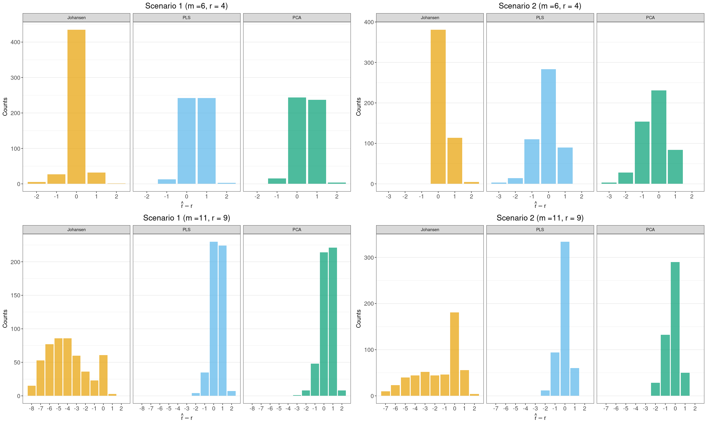
Figure 1: We contrast the differences between Scenario 1 (cointegrated series) with Scenario 2 in the dimension estimation error $\hat{r}-r$ for $(m,r)=(11,9),(6,4)$ using histograms.

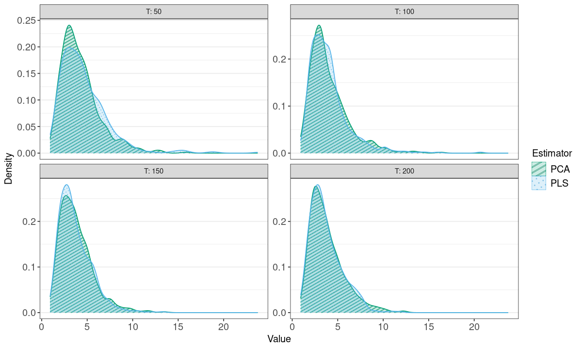
Figure 1: Visualisation of the distribution of $T\lVert P_{\beta_{\perp}}\hat{\beta}\rVert$ under Assumption 2 for PCA and PLS methods considering $S=500$, $m=11$ and $r=9$.

It is of interest to visualise the two scenarios previously described: the first is the cointegration scenario, and the second scenario is illustrated by considering $(\left|M_{1}\right|,\left|M_{2}\right|)=(m-3,2)$. First, in Figure 1, we visualise the distribution of $\hat{r}-r$, where positive values indicate overestimation of the dimension, and negative values indicate estimation of a stable space of smaller dimension. In Figure 2, we additionally visualise the distribution of $\delta(\hat{\beta},\beta)$ for each methodology through violin diagrams

In both the distribution of $\hat{r}-r$ and the subspace error, we can see that the Johansen procedure is more sensitive to increases in dimension as well as to changes in the scenario, although under the cointegration and low-dimensional setting, it performs substantially better.

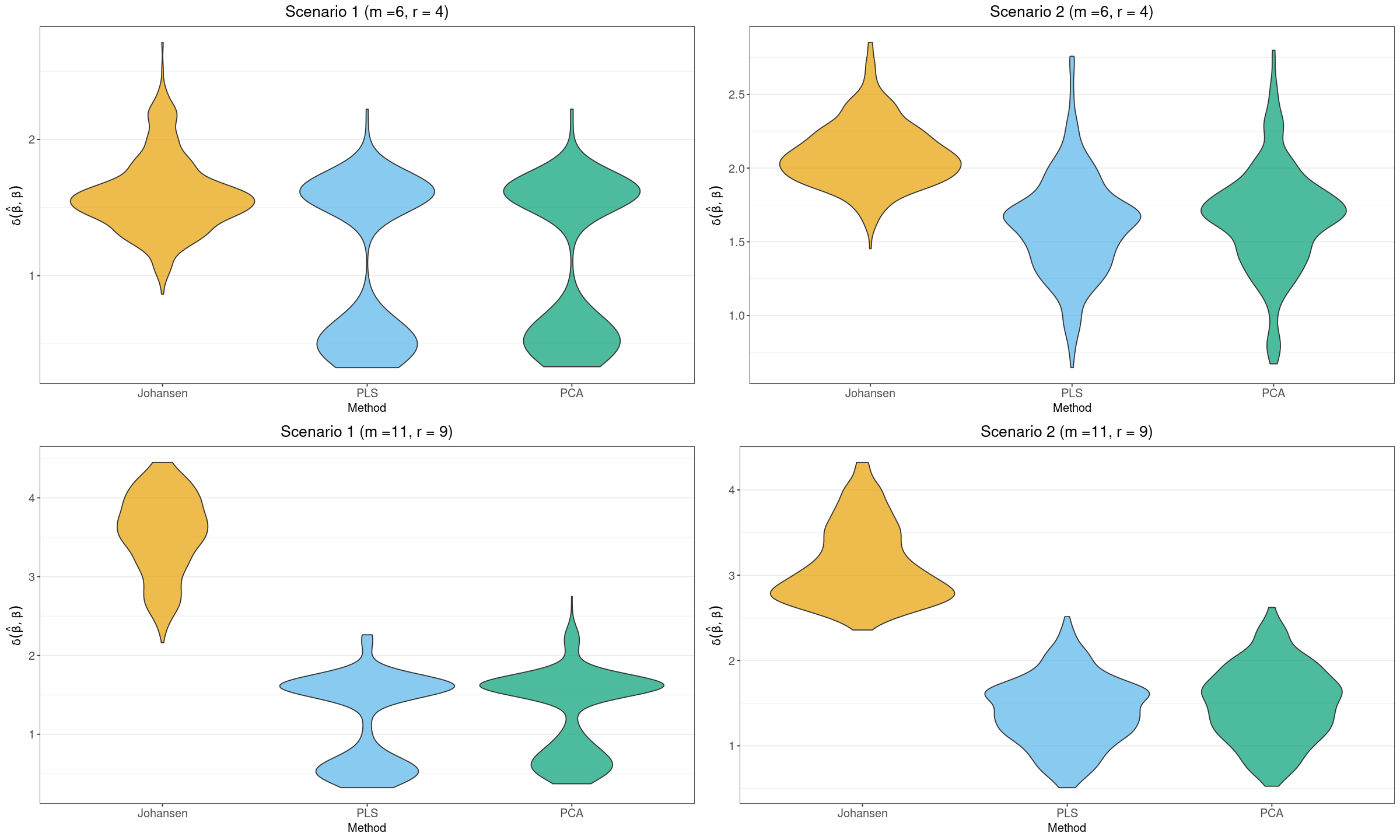
Figure 2: We contrast the differences between Scenario 1 (cointegrated series) with Scenario 2 in the stable space estimation error for $(m,r)=(11,9),(6,4)$ using violin diagrams.

For Case 1, which corresponds to the estimation of the cointegration space, as expected, all three methodologies yield consistent results for the different values of $r$, which can also be observed in Figure 1. Although the Johansen procedure is more accurate in estimating the dimension when $m=6$, we observe that as the value of $m$ increases, the estimation is severely affected. This is not the case for the PLS- and PCA-based methods, which maintain a more robust estimation of $r$ as the dimension increases. Thus, we see that the Johansen procedure struggles more in determining the dimension of the stable space as the scenario changes and the dimensionality increases.

Moreover, regarding the value of $\delta(\hat{\beta},\beta)$, Figure 2 shows similar performance across the three methodologies in the cointegration context. However, the Johansen procedure again exhibits poorer performance outside this setting compared to PLS and PCA, which in turn show comparable behaviour.

On the other hand, Table 2 summarises the results for $m=300$ with the suggested values for the dimension of the stable space $r$. As in the low-dimensional case, we observe a similar difference between the PCA- and PLS-based methodologies, but in this case with slightly better performance in favour of the PCA-based method.

Method	$r$	Case 1	Case 2	Case 3	Case 4
PCA	250	10.811 (0.075)	10.648 (0.137)	10.359 (0.172)	9.979 (0.249)
PLS	250	15.902 (0.071)	15.653 (0.070)	15.594 (0.055)	15.707 (0.065)
PCA	200	15.538 (0.028)	15.481 (0.075)	15.233 (0.148)	14.837 (0.242)
PLS	200	18.147 (0.039)	17.947 (0.034)	17.918 (0.040)	17.987 (0.035)
PCA	150	19.100 (0.024)	19.057 (0.056)	18.799 (0.148)	18.331 (0.232)
PLS	150	20.364 (0.027)	20.221 (0.025)	20.214 (0.025)	20.254 (0.032)

Table 2: Comparison of PLS, and PCA subspace estimation error with $m=300$ and $T=100$ across different cases and $r$ values. We add in parenthesis the standard deviation through the $S=100$ simulations.

Therefore, these methodologies offer a practical and efficient alternative for estimating the stable space in high-dimensional settings. To generate all tables and plots from the simulation study, we use the code provided in B, available via a GitHub repository link. In what follows, we illustrate the estimation and practical use of the stable space through real-world examples.

6 Practical Examples

6.1 Low-dimensional example

In the low-dimensional practical example, we analyse the behaviour of several economic indicators associated with inflation in Mexico. These variables form a vector time series $X$, and are described in Table 3.

Variables	Description
P	National Consumer Price Index (INEGI)
U	Unemployment Rate (INEGI)
BYM	Banknotes and Coins (Banxico)
E	Nominal Exchange Rate (INEGI)
R	28-Day Interbank Interest Rate (Banxico)
W	Real Wages (Banxico)
PUSA	United States National Consumer Price Index (BLS)

Table 3: Variables that make up the vector series related to inflation in Mexico. In parentheses, we indicate the public source from which the indicator comes.

The data, obtained from the National Institute of Statistics and Geography (INEGI, by its Spanish acronym) in Mexico, Banxico (Mexico’s central bank), and the U.S. Bureau of Labour Statistics (BLS), cover the period from January 2005 to January 2023, with monthly frequency. The compiled dataset is available in our GitHub repository; see B. This yields a random sample $\{X_{n},n=1,\dots,T\}$, with $m=7$ and $T=216$.

Following the information in Table 3, where P denotes the price level, each time series can be interpreted in relation to P as follows: U is associated with a Phillips curve relationship; BYM and R capture the link between prices and excess money in circulation, with the interest rate acting as an anchor to contain inflation. E and W represent input and wage costs faced by firms, while PUSA may be related to imported inflation. A similar study in this context is Bailliu et al. (2003), although it does not consider all these indicators jointly.

It is important to emphasise that no structural relationships are imposed in this analysis; instead, we explore the dynamics through both stable and unstable combinations across the panel of time series.

To approximate Assumption 1 as closely as possible, a preliminary analysis is conducted in which both the seasonal component and a linear trend are removed, as outlined in that assumption. For the BYM variable, the analysis is performed on the logarithmic scale.

For each of the series, a KPSS test can be conducted at the level of the series and after differencing, until there is no evidence to reject the null hypothesis. This allows for an empirical estimation of the order of integration of each series.

The results are summarised in Table 4, which shows the p-values obtained from the KPSS test for each corresponding series.

Variable	X	$\Delta X$	$\Delta^{2}X$
P	0.01	0.04	✓
U	0.02	✓	-
BYM	✓	-	-
E	✓	-	-
R	0.02	✓	-
W	0.01	0.04	✓
PUSA	✓	-	-

Table 4: p-value of the KPSS test applying to each coordinate of the original series $\{X_{n},n=1,\dots,T\}$ and considering one and two differences. The ✓indicates when the null hypothesis was not rejected using a $5\%$ significance level, and the - indicates that a hypothesis test was not done.

From Table 4, we can deduce the following:

• The variables BYM, E, and PUSA correspond to $\textsf{I}(0)$ series.

• The series associated with variables U and R are $\textsf{I}(1)$.

• The variables P and W are $\textsf{I}(2)$ series.

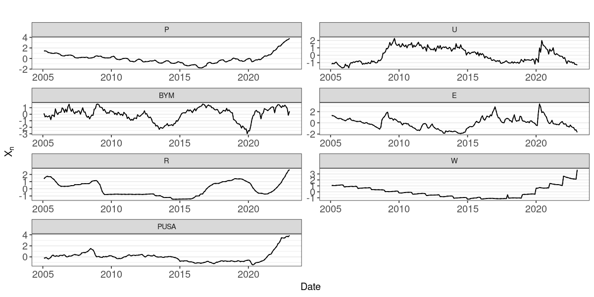
Figure 3: Visualisation of each time series corresponding to the economic indicators in Table 3.

Thus, there is evidence indicating that the vector series formed by these variables has components with different orders of integration, i.e., this example falls under Scenario 2. In Figure 3, we can observe the dynamics of each of these economic indicators after preprocessing.

We estimate a basis for the stable space using each of the three methodologies for the economic indicator series $\{X_{n},n=1,\dots,T\}$. It is important to note that the stationary scores also decompose the information into orthogonal factors; therefore, it is of interest to understand the contribution of each variable in constructing these scores.

For the Johansen and PCA procedures, the columns of $\hat{\beta}$ obtained are directly the weights that define the corresponding scores at the series level. However, for the PLS-based methodology, the columns of $\hat{\beta}$ must be transformed as described in Proposition 4.2.

Taking this into account, we can visualise the weights associated with each economic indicator by component in Figure 4.

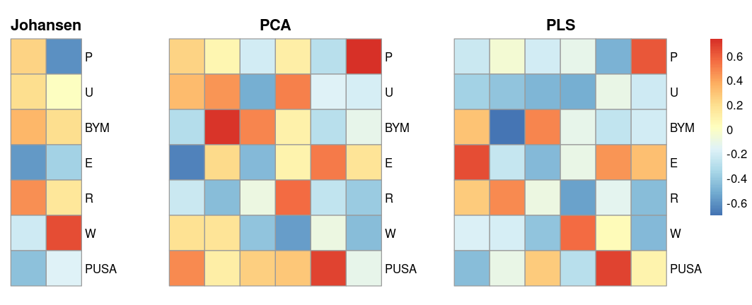
Figure 4: Heatmap that represents the weights of each variable in Table 3 on the stable scores construction.

We observe that, for the Johansen procedure, the first component assigns the highest weight to variable E, while the second component places most of the weight on variables P and W, and a stable space of dimension 2 is estimated.

On the other hand, for the PLS- and PCA-based methodologies, the estimated dimension of the stable space is 6. Although we have validated in the simulation study that both methods yield similar results, we observe that the components assign different weights to the variables in constructing the corresponding scores.

This may affect interpretation, particularly for some components. We observe that the key difference between PLS and PCA lies in the sign. This could not be seen in the simulation study, as the metrics used to evaluate the methodologies are sign-invariant.

In general, the problem of estimating the associated signs is challenging. For instance, Horváth and Kokoszka (2012) notes that in PCA, signs cannot be estimated from the data. This opens up the possibility of formalising whether this is feasible with PLS. Indeed, as shown, for example, in Bastien et al. (2005), the coordinates $\hat{w}_{i}$ correspond to the partial correlations between $X_{n}$ and $X_{n-1}$ given $T_{1},\dots,T_{i-1}$, which implies that the weights obtained via PLS have a direct interpretation in terms of dependence between $X_{n}$ and $X_{n-1}$. This is not the case for the PCA-based methodology, even if both methods estimate the same space.

On the other hand, PCA and PLS are dimensionality reduction methods. In practice, the first components are selected based on the idea that they capture the greatest variability of the observed information. This idea can also be applied here, with the additional consideration that these components should yield stationary scores, which is conceptually more appropriate.

Thus, we compare the projection error of the PCA- and PLS-based methodologies with the Johansen procedure in a dimensionality reduction context. For each method, we select the first two stationary scores, since only two components are available for the Johansen procedure. We then compute the projection of the original series onto the stationary scores using a regression model in the case of PCA and Johansen, and the decomposition in (8) for PLS.

Additionally, we consider the outcome of selecting the first two components without assessing whether they yield stationary scores. We illustrate this using PCA and refer to this method as classical PCA, in contrast to the proposed approach, which involves selecting the leading stable components and is referred to as stationary PCA (or stationary PLS, where applicable). In this context, the classical PCA approach corresponds to the selection of one non-stationary component associated with the first principal component, along with the first stationary component.

After selecting the corresponding scores and performing the projection, we compute the error between the observed series and its projection. Specifically, we calculate the mean squared error (MSE) for each series, normalised with respect to its sample variance.

Variable	Johansen	classic PCA	stationary PCA	stationary PLS
P	0.99	0.07	0.88	0.90
U	0.99	0.44	0.65	0.63
BYM	0.98	0.67	0.36	0.35
E	0.84	0.24	0.25	0.24
R	0.97	0.28	0.70	0.68
W	0.90	0.22	0.90	0.92
PUSA	1.00	0.11	0.56	0.60

Table 5: Normalised MSE of the projection onto the main two stationary scores for each method, and against considering the first two principal components regardless of their stability

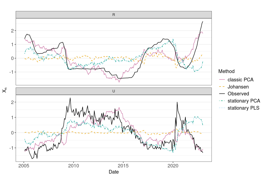
Figure 5: Visualisation of the scaled U and R indicators projection onto the two main stability components. For PCA, we also consider the projection on the two main principal components regardless of stability.

These errors are reported in Table 5. We observe that the Johansen procedure performs worse compared to the other methodologies across all series. On the other hand, PLS and stationary PCA yield similar results, while classical PCA –although showing better performance– does so by capturing the non-stationary aspects of the observed sample, due to the non-stability of the first principal component.

Finally, in Figure 5, we visualise the projection for each of the methodologies and approaches, for example, focusing on the variables U and R, where the difference in error between the Johansen procedure and PCA/PLS is greatest. Moreover, we can observe the non-stationary aspects captured by including the first non-stable principal component in classical PCA, and the contrast with selecting the first two stable components.

Although classical PCA provides a good fit within the sample range, stationary PCA exhibits extrapolation capability and captures the most relevant stationary part of each series, yielding a better fit in some regions than in others. The regions where the difference between the stationary projection and the observed series is largest could be interpreted as periods where the process deviates most from stationarity, opening the door to investigating the underlying causes.

6.2 High-dimensional example

We now analyse $m=205$ monthly series retrieved from the indicators database provided by INEGI. Specific information about these series can be found in the catalogues available in the repository referenced in B, along with the dataset itself. Some of the variables included in this database are the unemployment rate, indicators of economic activity in the construction sector (variable s23 in the dataset), and the professional, scientific, and technical services sector (variable s54 in the dataset).

We apply the same preprocessing scheme to the data to obtain a process that satisfies, at a minimum, Assumption 1.

The information for each of the 205 economic indicators covers the period from January 2017 to December 2024, that is, $T=95$. Therefore, we are in the case where $T<m$.

In the same way as in the low-dimensional setting, we identify the order of integration of each series using the KPSS test. Among the 205 series in the system, we find that 185 are identified as $\textsf{I}(0)$, 19 as $\textsf{I}(1)$, and one as $\textsf{I}(2)$.

Thus, we would expect the estimated dimension of the stable space to be at least 185, although it could be higher if there are components that compensate across all series –including the non-stationary ones– to produce stationary scores.

The estimators $\hat{\beta}_{\text{PLS}}$ and $\hat{\beta}_{\text{PCA}}$ are computed using a significance level of $5\%$ for detecting the stable components. We obtain $\dim\text{Col }\hat{\beta}_{\text{PLS}}=191$, while $\dim\text{Col }\hat{\beta}_{\text{PCA}}=199$, so the dimensions of the estimated non-stable spaces are 14 and 6, respectively.

In this case, for both the PLS and PCA methodologies, the first two stable components coincide with the first two components obtained by each method, i.e., the stationary approach aligns with the classical one. This illustrates that when Assumption 2 does not hold, it is necessary to identify the stable components explicitly, even if they do not appear in order.

Therefore, we see that although the multivariate series includes non-stationary components, the majority of series identified as $\textsf{I}(0)$ dominate the variance/covariance structure of the system. As a result, the first components obtained by the methodologies are stable.

To illustrate the difference between stable and non-stable components, we consider the approximation of the observed data using the first two components in each case. When using the stable components, we refer to the stationary approach, while the approximation based on the first two non-stable components is referred to as the non-stable version of the method.

Variable	PCA non-stable	PCA stationary	PLS non-stable	PLS stationary
s23	0.99	0.26	0.98	0.25
imaief_Hgo	0.98	0.43	0.98	0.42
imaief_SLP	0.98	0.51	0.98	0.51
s54	0.99	0.42	0.99	0.43
rem_cmenor	0.98	0.17	0.99	0.17

Table 6: Normalised MSE of the projection onto the main two stationary scores and the two main non-stable components on some series in the system. The rem_cmenor is the $\textsf{I}(2)$ serie whereas the rest are $\textsf{I}(1)$ series.

In Table 6, we present the normalised MSE for several series in the system. s23 represents the construction indicator, s54 corresponds to professional and scientific services, imaief_Hgo and imaief_SLP represent industrial activity indicators for the Mexican states of Hidalgo and San Luis Potosí, respectively, and rem_cmenor is the retail trade indicator.

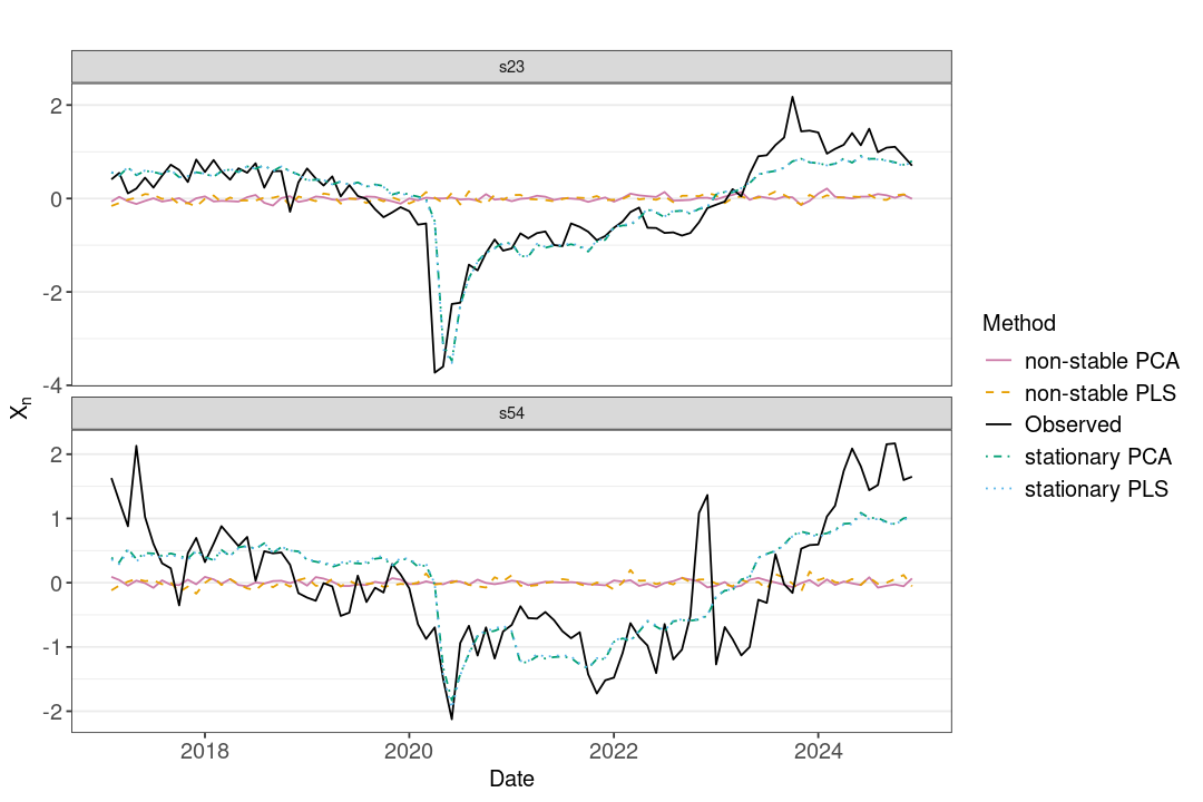
Figure 6: Visualisation of the scaled s23 and s54 indicators projection onto the two main stability components and the first two non-stable components.

We observe that the stationary approach yields a lower error than the non-stationary one, even though all the series shown in Table 6 are non-stationary. Consequently, the first two stable components –which in this case coincide with the first two overall components– not only load on the stationary components but also on the non-stationary ones in such a way as to construct the corresponding stationary scores.

This last phenomenon somewhat contradicts the previous example. It may be due either to the larger number of $\textsf{I}(0)$ components, as previously mentioned, or to the curse of dimensionality. In this case, it may be appropriate to consider regularisation techniques.

As in the previous section, in Figure 6 we visualise the projection for the series s23 and s54, confirming that the adjustment provided by the stable components –which combine all the information– offers a better approximation to the observed series than using the first two non-stable components, despite the non-stationarity of the respective scores.

The data and the code for reproducing the results can be found in B.

7 Discussion

The cointegration framework proposed by Engle and Granger (1987) and formalised in the Johansen procedure (Johansen, 1991) constitutes one of the main tools for addressing non-stationarity in multivariate time series. However, as demonstrated, its practical applicability in high-dimensional settings is limited due to its computational complexity, its parametric nature, and –as shown in this work– the restrictive assumption of a cointegrated system of series.

In contrast, methodologies based on non-parametric dimensionality reduction techniques, such as PCA and PLS, offer a more flexible and efficient way to address the inherent complexity of systems with a large number of variables. While these methodologies can initially be applied within a cointegration framework, we have shown that they are capable of recovering the most relevant aspects of the underlying stationary dynamics through stationary scores in a more flexible setting.

The concept of a stable space, introduced in this work, is proposed as a natural and less restrictive extension of the cointegration space. This notion allows the identification of linear combinations of the original series that generate processes with stationary behaviour. In doing so, it broadens the range of situations in which it is possible to apply analytical techniques based on the assumption of stationarity, enhancing both the applicability and robustness of statistical procedures.

A key methodological proposal of this work is the use of components associated with the stable space in the context of dimensionality reduction. While these components do not necessarily correspond to those that maximise explained variance –as in classical principal components– they offer the significant advantage of being stationary. This property provides, on the one hand, an alternative and lower-complexity representation of the data, and on the other, the ability to apply statistical techniques that require stationarity, such as VAR models, forecasting methods, or changepoint detection techniques.

The results of the simulation study, carefully designed to assess the performance of the different methodologies under a variety of scenarios (including explicit cointegration structures, low- and high-dimensional configurations, and partially violated assumptions), support the effectiveness of the proposed approach. In particular, the estimation of the stable space via PCA and PLS proves robust across the proposed scenarios, which represent deviations from classical assumptions. Furthermore, these methods are capable of capturing relevant information in a parsimonious manner.

Finally, it is important to highlight that the approach developed in this work opens multiple avenues for future research. One of the most promising consists in generalising the concept of stable space to nonlinear contexts or more complex forms of temporal dependence. In this regard, the core idea behind the PLS algorithm –based on capturing linear dependence between $X_{n}$ and $X_{n-1}$– provides a natural starting point for building nonlinear extensions. It is also of great interest to explore the application of this approach in specific domains in conjunction with other methodologies –such as prediction or changepoint detection– in areas such as macroeconomics, financial analysis, or the study of multivariate biological systems, where the simultaneous presence of high dimensionality and non-stationarity is common.

Funding

This work was supported by the Project CBF2023-2024-3976, sponsored by the Mexican Secretariat of Science, Humanities, Technology, and Innovation (SECIHTI). Roberto Vásquez Martínez was also supported by the EPSRC-funded STOR-i Centre for Doctoral Training [grant number EP/Y035305/1].

Declaration of generative AI and AI-assisted technologies in the writing process

During the preparation of this work, the author(s) used ChatGPT, a language model developed by OpenAI, to assist with the writing and editing process. After using this tool/service, the author(s) reviewed and edited the content as needed and take(s) full responsibility for the content of the published article.

Appendix A Proofs of Theoretical Results

Proof of Proposition 2.2: This proof is based on that given in Lütkepohl (2005), Proposition 6.1, and follows the same notation.

First, we consider the parametrisation of the polynomial $\theta$ as

$$\theta(z)=\theta(1)+(1-z)\theta^{\star}(z),$$

so that

$$Z_{n}=\theta(1)\epsilon_{n}+\theta^{\star}(B)\Delta\epsilon_{n}.$$ (9)

On the other hand, since $P_{\beta_{\perp}}Z_{n}=P_{\beta_{\perp}}\Delta X_{n}$, we have

$$X_{n} =\sum_{i=1}^{n}\Delta X_{i}$$

$$=\sum_{i=1}^{n}(P_{\beta}\Delta X_{i}+P_{\beta_{\perp}}\Delta X_{i})$$

$$=\sum_{i=1}^{n}P_{\beta_{\perp}}Z_{i}+\sum_{i=1}^{n}P_{\beta}\Delta X_{i}$$

$$=\sum_{i=1}^{n}P_{\beta_{\perp}}Z_{i}+P_{\beta}X_{n}.$$

From the last expression and the reparametrisation (9), we obtain:

$$X_{n} =P_{\beta_{\perp}}\theta(1)\sum_{i=1}^{n}\epsilon_{i}+P_{\beta_{\perp}}\theta^{\star}(B)\sum_{i=1}^{n}\Delta\epsilon_{i}+P_{\beta}X_{n}$$

$$=P_{\beta_{\perp}}\left(\theta(1)\sum_{i=1}^{n}\epsilon_{i}\right)+P_{\beta_{\perp}}\theta^{\star}(B)\epsilon_{n}+P_{\beta}X_{n}.$$ (10)

Let $\eta_{n}:=P_{\beta_{\perp}}\theta^{\star}(B)\epsilon_{n}$. Note that $\{\eta_{n},n\in\mathbb{N}\}$ is a stationary time series, and from this and (10), the result follows.

Proof of Lemma 4.1: First, note that

$$(\hat{w}_{1},\hat{c}_{1})=\operatorname{argmax}_{d\in\mathbb{R}^{m}}\operatorname{argmax}_{e\in\mathbb{R}^{m}}\operatorname{Cov}(\mathbf{X}d,\mathbf{Y}e)^{2}.$$ (11)

Now, let us fix $d$ with $\lVert d\rVert=1$ and consider the optimisation problem

$$\hat{c}(d)=\operatorname{argmax}_{e\in\mathbb{R}^{m}}\operatorname{Cov}(\mathbf{X}d,\mathbf{Y}e)^{2}\quad\text{subject to }\lVert e\rVert=1,$$

that is, we fix one variable and maximise with respect to the other.

On the other hand, observe that

$$\operatorname{Cov}(\mathbf{X}d,\mathbf{Y}e)^{2} \propto(d^{\prime}\mathbf{X}^{\prime}\mathbf{Y}e)^{2}$$

$$=\langle\mathbf{Y}^{\prime}\mathbf{X}d,e\rangle^{2},$$

where $\langle\cdot,\cdot\rangle$ denotes the inner product in $\mathbb{R}^{m}$.

By the Cauchy–Schwarz inequality:

$$\langle\mathbf{Y}^{\prime}\mathbf{X}d,e\rangle^{2}\leq\lVert\mathbf{Y}^{\prime}\mathbf{X}d\rVert^{2}\cdot\lVert e\rVert^{2}=\lVert\mathbf{Y}^{\prime}\mathbf{X}d\rVert^{2},$$

since $\lVert e\rVert=1$.

As $d$ is fixed and the right-hand side of the inequality does not depend on $e$, the maximum of $\operatorname{Cov}(\mathbf{X}d,\mathbf{Y}e)^{2}$ is attained when $e\propto\mathbf{Y}^{\prime}\mathbf{X}d$, according to the equality condition of the Cauchy–Schwarz inequality.

Therefore, the optimisation problem in (11) simplifies to

$$\hat{w}_{1} =\operatorname{argmax}_{d\in\mathbb{R}^{m}}\operatorname{Cov}(\mathbf{X}d,\mathbf{Y}\mathbf{Y}^{\prime}\mathbf{X}d)^{2}$$

$$=\operatorname{argmax}_{d\in\mathbb{R}^{m}}(d^{\prime}\mathbf{X}^{\prime}\mathbf{Y}\mathbf{Y}^{\prime}\mathbf{X}d)^{2}\quad\text{subject to }\lVert d\rVert=1,$$

so that $\hat{w}_{1}$ is the eigenvector associated with the largest eigenvalue $\lambda^{2}>0$ of the matrix $\mathbf{X}^{\prime}\mathbf{Y}\mathbf{Y}^{\prime}\mathbf{X}$, and

$$\hat{c}_{1}\propto\mathbf{Y}^{\prime}\mathbf{X}\hat{w}_{1}.$$

Moreover, if $\hat{c}_{1}=k\cdot\mathbf{Y}^{\prime}\mathbf{X}\hat{w}_{1}$ and $\lVert\hat{c}_{1}\rVert=1$, then:

$$1 =k^{2}\cdot\hat{w}_{1}^{\prime}\mathbf{X}^{\prime}\mathbf{Y}\mathbf{Y}^{\prime}\mathbf{X}\hat{w}_{1}$$

$$=k^{2}\cdot\hat{w}_{1}^{\prime}(\lambda^{2}\hat{w}_{1})$$

$$=k^{2}\cdot\lambda^{2},$$

since $\lVert\hat{w}_{1}\rVert=1$. Thus, the proportionality constant in the relation $\hat{c}_{1}\propto\mathbf{Y}^{\prime}\mathbf{X}\hat{w}_{1}$ is $k=\lambda^{-1}$, i.e., the reciprocal of the largest singular value of the sample cross-covariance matrix $\mathbf{Y}^{\prime}\mathbf{X}$.

Proof of Proposition 4.2: This result is proven by mathematical induction on $i$, the iteration number.

For $i=1$, if $A_{1}=I_{m}$, the identity matrix in $\mathbb{R}^{m}$, then $\mathbf{X}^{(1)}=\mathbf{X}^{(1)}A_{1}$, so the result holds in this case.

Suppose the result holds for $i$. Consider $i<m$, and we will prove the result for $i+1$.

Note that,

$$\mathbf{X}^{(i+1)}=\mathbf{X}^{(i)}P_{i}.$$

By the induction hypothesis, we have $\mathbf{X}^{(i)}=\mathbf{X}^{(1)}A_{i}$, so

$$\mathbf{X}^{(i+1)}=\mathbf{X}^{(1)}A_{i}P_{i},$$

thus, define $A_{i+1}=A_{i}P_{i}$ and the result holds for $i+1$, which concludes the induction.

Since $A_{i+1}=A_{i}P_{i}$ and $A_{1}=I_{m}$, it follows by recursion that

$$A_{i+1}=P_{1}\cdots P_{i}\quad\text{for }i=1,2,\dots,m-1,$$

which gives the explicit form of the transformation used to obtain the weights in the scale of the original information $\mathbf{X}^{(1)}$.

Thus,

$$T_{i}=\mathbf{X}^{(i)}\hat{w}_{i}=\mathbf{X}^{(1)}A_{i}\hat{w}_{i}=\mathbf{X}^{(1)}\hat{\gamma}_{i},$$

which is the expression of the scores as a linear combination of the original variables.

Proof of Remark 3: We know that for $i=0,1,\dots,m-1$

$$\hat{w}_{i+1}=\operatorname{argmax}_{d}d^{\prime}\tilde{S}_{i+1}^{\prime}\tilde{S}_{i+1}d\quad\text{ with }\lVert d\rVert=1,$$ (12)

where

$$\tilde{S}_{i+1}:=T^{-1}(\mathbf{X}^{(i+1)})^{\prime}(\mathbf{Y}^{(i+1)}).$$

A simplifying assumption of Algorithm 1, as noted in Höskuldsson (1988), is to omit the update for the response variable in step 4.

This is due to the fact that

$$(\mathbf{Y}^{(i+1)})^{\prime}T_{i+1}=\mathbf{Y}^{\prime}T_{i+1},$$

which implies

$$\mathbf{Y}^{(i+1)}=\underbrace{\left[I_{T-1}-\sum_{j=1}^{i}\frac{T_{j}T_{j}^{\prime}}{T_{j}^{\prime}T_{j}}\right]}_{B_{i+1}}\mathbf{Y}.$$

Furthermore, one can verify that a similar update holds for the covariates, i.e., $\mathbf{X}^{(i+1)}=B_{i+1}\mathbf{X}$, thus

$$\tilde{S}_{i+1}^{\prime}\tilde{S}_{i+1} \propto(\mathbf{X}^{(i+1)})^{\prime}\mathbf{Y}^{(i+1)}(\mathbf{Y}^{(i+1)})^{\prime}\mathbf{X}^{(i+1)}$$

$$=\mathbf{X}^{\prime}B_{i+1}^{\prime}\mathbf{Y}\mathbf{Y}^{\prime}B_{i+1}\mathbf{X}$$

$$=(\mathbf{X}^{(i+1)})^{\prime}\mathbf{Y}\mathbf{Y}^{\prime}\mathbf{X}^{(i+1)}.$$

In this way, the algorithm is simplified by considering only the residual update for the covariate matrix $\mathbf{X}$.

Proof of Proposition 4.3: The idea of the proof is to use Lemma 1 from Harris (1997), that is, to relate the decomposition obtained via PCA with that obtained via the PLS algorithm.

Let $\mathbf{X}$ and $\mathbf{Y}$ be as in (4), and consider the estimators of the asymptotic covariances:

$$S_{XY}:=T^{-1}\mathbf{X}^{\prime}\mathbf{Y}=T^{-1}\sum_{i=2}^{T}X_{i-1}X_{i}^{\prime},$$

and

$$S_{YX}:=T^{-1}\mathbf{Y}^{\prime}\mathbf{X}=T^{-1}\sum_{i=2}^{T}X_{i}X_{i-1}^{\prime}.$$

By hypothesis, we know that $\{X_{n},n=1,\dots,T\}$ satisfies the conditions of the Granger Representation Theorem, so that

$$X_{n}=N_{n}+\eta_{n}+X_{0}^{\star},$$

with $N\sim\textsf{I}(1)$, $\eta\sim\textsf{I}(0)$, and $X_{0}^{\star}$ a constant.

Since we are interested in an asymptotic result, we may assume without loss of generality that $X_{0}^{\star}=0$.

From the above, we obtain

$$S_{XY}=T^{-1}\left(\sum_{i=2}^{T}N_{i-1}N_{i}^{\prime}+\sum_{i=2}^{T}N_{i-1}\eta_{i}+\sum_{i=2}^{T}\eta_{i-1}N_{i}^{\prime}+\sum_{i=2}^{T}\eta_{i-1}\eta_{i}^{\prime}\right).$$ (13)

Specifically, by Theorem 2.1, we have

$$\eta_{n}=\mathfrak{F}^{\star}(B)\epsilon_{n}=\sum_{i=0}^{\infty}\mathfrak{F}^{\star}_{i}\epsilon_{n-i},\quad\text{and}\quad N_{n}=\mathfrak{F}\cdot\sum_{i=1}^{n}\epsilon_{i}.$$

From Theorem B.13 of Johansen (1995) we get

$$\sum_{i=2}^{T}N_{i-1}N_{i}^{\prime} =\sum_{i=2}^{T}N_{i-1}N_{i-1}^{\prime}+O_{p}(T),$$

$$\sum_{i=2}^{T}N_{i-1}\eta_{i}^{\prime} =O_{p}(T),$$

$$\sum_{i=2}^{T}\eta_{i-1}N_{i}^{\prime} =O_{p}(T),$$

$$T^{-1}\sum_{i=2}^{T}\eta_{i-1}\eta_{i}^{\prime} =\hat{\Sigma}_{\eta}(1)+o_{p}(1),$$

where $\hat{\Sigma}_{\eta}(1)$ is the sample estimator of the lag-1 autocovariance function of the process $\eta$.

From these and (13), it follows that

$$S_{XY}=T^{-1}\sum_{i=2}^{T}N_{i-1}N_{i-1}^{\prime}+\hat{\Sigma}_{\eta}(1)+O_{p}(1).$$

Similarly, we obtain

$$S=T^{-1}\sum_{i=1}^{T}N_{i}N_{i}^{\prime}+\hat{\Sigma}_{\eta}(0)+O_{p}(1).$$

Let $\tilde{S}_{XY}:=T^{-1}S_{XY}$, $\tilde{S}_{YX}:=T^{-1}S_{YX}$, and $\tilde{S}:=T^{-1}S$, then

$$\tilde{S}_{XY}=T^{-2}\sum_{i=2}^{T}N_{i-1}N_{i-1}^{\prime}+o_{p}(1),\quad\text{and}\quad\tilde{S}=T^{-2}\sum_{i=1}^{T}N_{i}N_{i}^{\prime}+o_{p}(1).$$

This follows from the fact that $T^{-1}\to 0$ as $T\to\infty$, hence

$$T^{-1}\hat{\Sigma}_{\eta}(i)=o_{p}(1)\text{ for }i=0,1,\quad\text{and}\quad T^{-1}O_{p}(1)=o_{p}(1)O_{p}(1)=o_{p}(1).$$

Thus, we get

$$\tilde{S}_{XY}=\tilde{S}+o_{p}(1),\quad\text{and}\quad\tilde{S}_{YX}=\tilde{S}+o_{p}(1).$$ (14)

In Engle and Granger (1987) it is stated that $\mathbb{E}[T^{-1}S]$ converges to a non-zero matrix, which implies $\tilde{S}=O_{p}(1)$. From this and (14), we have

$$\tilde{S}_{XY}\tilde{S}_{YX}=\tilde{S}^{2}+o_{p}(1).$$

On the other hand, note that the first PLS component $\hat{w}_{1}$ satisfies the eigenvalue problem

$$\tilde{S}_{XY}\tilde{S}_{YX}\hat{w}_{1}=\lambda_{1}\hat{w}_{1}.$$

Since $\tilde{S}_{XY}\tilde{S}_{YX}$ is asymptotically equivalent to $\tilde{S}^{2}$, and the eigenvalue problem is invariant under scalar multiplication, we have that in the limit $\hat{w}_{1}$ corresponds to the first eigenvector of $\tilde{S}^{2}$, i.e., the first principal component.

Hence, we may consider $P_{1}\approx I_{m}-\hat{w}_{1}\hat{w}_{1}^{\prime}$, and then the next step of Algorithm 1 corresponds to solving the eigenvalue problem:

$$P_{1}\tilde{S}_{XY}\tilde{S}_{YX}P_{1}\hat{w}_{2}=\lambda_{2}\hat{w}_{2},$$

and $P_{1}\tilde{S}_{XY}\tilde{S}_{YX}P_{1}$ is asymptotically equivalent to $P_{1}\tilde{S}^{2}P_{1}$, so in the limit $\hat{w}_{2}$ is the first eigenvector of $P_{1}S^{2}P_{1}$, i.e., the second principal component.

An inductive argument implies that in the $i$th iteration, the first eigenvector of $A_{i}\tilde{S}_{XY}\tilde{S}_{YX}A_{i}$ is asymptotically equivalent to the first eigenvector of $A_{i}\tilde{S}^{2}A_{i}$, which corresponds to the $i$th principal component.

Thus, we have

$$\hat{\beta}_{\textsc{PLS}}=\hat{\beta}_{\textsc{PCA}}+o_{p}(1).$$

Hence,

$$P_{\beta_{\perp}}\hat{\beta}_{\textsc{PLS}}=P_{\beta_{\perp}}\hat{\beta}_{\textsc{PCA}}+o_{p}(1),$$

and by Lemma 1 of Harris (1997) we have $P_{\beta_{\perp}}\hat{\beta}_{\textsc{PCA}}=O_{p}(T^{-1})$, so that

$$P_{\beta_{\perp}}\hat{\beta}_{\textsc{PLS}}=O_{p}(T^{-1}),$$

which concludes the proof.

Appendix B Software

Link to a GitHub repository with all the source code for reproducing the tables and plots of the paper: ts_stable_space.

References

- Adak (1998) Adak, S., 1998. Time-Dependent Spectral Analysis of Nonstationary Time Series. Journal of the American Statistical Association 93, 1488–1501. doi:10.1080/01621459.1998.10473808.
- Bailliu et al. (2003) Bailliu, J., Garcés, D., Kruger, M., Messmacher, M., 2003. Explaining and Forecasting Inflation in Emerging Markets: The Case of Mexico doi:10.34989/SWP-2003-17. publisher: Bank of Canada.
- Bastien et al. (2005) Bastien, P., Vinzi, V.E., Tenenhaus, M., 2005. PLS Generalised Linear Regression. Computational Statistics & Data Analysis 48, 17–46. doi:10.1016/j.csda.2004.02.005.
- Bhaskaran et al. (2013) Bhaskaran, K., Gasparrini, A., Hajat, S., Smeeth, L., Armstrong, B., 2013. Time Series Regression Studies in Environmental Epidemiology. International Journal of Epidemiology 42, 1187–1195. doi:10.1093/ije/dyt092.
- Davidson et al. (1978) Davidson, J.E.H., Hendry, D.F., Srba, F., Yeo, S., 1978. Econometric Modelling of the Aggregate Time-Series Relationship Between Consumers’ Expenditure and Income in the United Kingdom. The Economic Journal 88, 661. doi:10.2307/2231972.
- Dickey et al. (1986) Dickey, D.A., Bell, W.R., Miller, R.B., 1986. Unit Roots in Time Series Models: Tests and Implications. The American Statistician 40, 12–26. doi:10.1080/00031305.1986.10475349.
- Dickey and Pantula (1987) Dickey, D.A., Pantula, S.G., 1987. Determining the Order of Differencing in Autoregressive Processes. Journal of Business & Economic Statistics 5, 455–461. doi:10.1080/07350015.1987.10509614.
- Engle and Granger (1987) Engle, R.F., Granger, C.W.J., 1987. Co-Integration and Error Correction: Representation, Estimation, and Testing. Econometrica 55, 251. doi:10.2307/1913236.
- Garthwaite (1994) Garthwaite, P.H., 1994. An Interpretation of Partial Least Squares. Journal of the American Statistical Association 89, 122–127. doi:10.1080/01621459.1994.10476452.
- Gonzalo and Lee (1998) Gonzalo, J., Lee, T.H., 1998. Pitfalls in Testing for Long Run Relationships. Journal of Econometrics 86, 129–154. doi:10.1016/S0304-4076(97)00111-5.
- Hamilton (1989) Hamilton, J.D., 1989. A New Approach to the Economic Analysis of Nonstationary Time Series and the Business Cycle. Econometrica 57, 357. doi:10.2307/1912559.
- Hamilton (2020) Hamilton, J.D., 2020. Time Series Analysis. Princeton University Press.
- Harris (1997) Harris, D., 1997. Principal Components Analysis of Cointegrated Time Series. Econometric Theory 13, 529–557. doi:10.1017/S0266466600005995.
- Horváth and Kokoszka (2012) Horváth, L., Kokoszka, P., 2012. Inference for Functional Data with Applications. Springer-Verlag.
- Hotelling (1933) Hotelling, H., 1933. Analysis of a complex of statistical variables into principal components. Journal of Educational Psychology 24, 417–441. doi:10.1037/h0071325. place: US Publisher: Warwick & York.
- Huang and Yang (1996) Huang, B.N., Yang, C.W., 1996. Long-run Purchasing Power Parity Revisited: a Monte Carlo Simulation. Applied Economics 28, 967–974. doi:10.1080/000368496328092.
- Höskuldsson (1988) Höskuldsson, A., 1988. PLS Regression Methods. Journal of Chemometrics 2, 211–228. doi:10.1002/cem.1180020306.
- James et al. (2012) James, S.L., Gubbins, P., Murray, C.J., Gakidou, E., 2012. Developing a Comprehensive Time Series of GDP per Capita for 210 Countries from 1950 to 2015. Population Health Metrics 10, 12. doi:10.1186/1478-7954-10-12.
- Johansen (1991) Johansen, S., 1991. Estimation and Hypothesis Testing of Cointegration Vectors in Gaussian Vector Autoregressive Models. Econometrica 59, 1551. doi:10.2307/2938278.
- Johansen (1995) Johansen, S., 1995. Likelihood-based Inference in Cointegrated Vector Autoregressive Models. Oxford University Press.
- Kaufmann et al. (2006) Kaufmann, R.K., Kauppi, H., Stock, J.H., 2006. Emissions, Concentrations, and Temperature: A Time Series Analysis. Climatic Change 77, 249–278. doi:10.1007/s10584-006-9062-1.
- Killick et al. (2012) Killick, R., Fearnhead, P., Eckley, I.A., 2012. Optimal Detection of Changepoints with a Linear Computational Cost. Journal of the American Statistical Association 107, 1590–1598. doi:10.1080/01621459.2012.737745.
- Kwiatkowski et al. (1992) Kwiatkowski, D., Phillips, P.C., Schmidt, P., Shin, Y., 1992. Testing the Null Hypothesis of Stationarity Against the Alternative of a Unit Root. Journal of Econometrics 54, 159–178. doi:10.1016/0304-4076(92)90104-Y.
- Lam et al. (2011) Lam, C., Yao, Q., Bathia, N., 2011. Estimation of Latent Factors for High-dimensional Time Series. Biometrika 98, 901–918. doi:10.1093/biomet/asr048.
- Lütkepohl (2005) Lütkepohl, H., 2005. New Introduction to Multiple Time Series Analysis. Springer Science & Business Media.
- Maddala and Kim (1998) Maddala, G.S., Kim, I.M., 1998. Unit Roots, Cointegration, and Structural Change. Cambridge University Press.
- Maharaj (2000) Maharaj, E., 2000. Cluster of Time Series. Journal of Classification 17, 297–314. doi:10.1007/s003570000023.
- Mahdi (2023) Mahdi, E., 2023. portes: Portmanteau Tests for Time Series Models. URL: https://CRAN.R-project.org/package=portes.
- Muriel et al. (2012) Muriel, N., González-Farías, G., Ramos, R., 2012. A PLS Based Approach to Cointegration Analysis. Journal of Business & Economics 4, 177–199.
- Osterwald-Lenum (1992) Osterwald-Lenum, M., 1992. A Note with Quantiles of the Asymptotic Distribution of the Maximum Likelihood Cointegration Rank Test Statistics. Oxford Bulletin of Economics & Statistics 54.
- Peña et al. (2019) Peña, D., Tsay, R.S., Zamar, R., 2019. Empirical Dynamic Quantiles for Visualization of High-Dimensional Time Series. Technometrics 61, 429–444. doi:10.1080/00401706.2019.1575285.
- Pfaff (2008) Pfaff, B., 2008. Analysis of Integrated and Cointegrated Time Series with R. Springer Science & Business Media.
- Qiu and Joe (2023) Qiu, W., Joe, H., 2023. clusterGeneration: Random Cluster Generation (with Specified Degree of Separation). URL: https://CRAN.R-project.org/package=clusterGeneration.
- Sargan (1964) Sargan, J.D., 1964. Wages and Prices in the United Kingdom: a Study in Econometric Methodology. Econometric Analysis for National Economic Planning 16, 25–54.
- Seo (2024) Seo, W., 2024. Functional Principal Component Analysis for Cointegrated Functional Time Series. Journal of Time Series Analysis 45, 320–330. doi:10.1111/jtsa.12707.
- Stock and Watson (2002) Stock, J.H., Watson, M.W., 2002. Forecasting Using Principal Components from a Large Number of Predictors. Journal of the American Statistical Association 97, 1167–1179. doi:10.1198/016214502388618960.
- Wold (1966) Wold, H., 1966. Estimation of Principal Components and Related Models by Iterative Least Squares. Multivariate Analysis , 391–420.
- Wold (1980) Wold, H., 1980. Model Construction and Evaluation When Theoretical Knowledge Is Scarce: Theory and Application of Partial Least Squares, in: Kmenta, J., Ramsey, J.B. (Eds.), Evaluation of Econometric Models. Academic Press, pp. 47–74. doi:10.1016/B978-0-12-416550-2.50007-8.
- Ye and Lim (2016) Ye, K., Lim, L.H., 2016. Schubert Varieties and Distances between Subspaces of Different Dimensions. SIAM Journal on Matrix Analysis and Applications 37, 1176–1197. doi:10.1137/15M1054201.