Asymptotic Inference for Exchangeable Gibbs Partitions

Abstract

We study the asymptotic properties of parameter estimation and predictive inference under the exchangeable Gibbs partition, characterized by a discount parameter $\alpha\in(0,1)$ and a triangular array $v_{n,k}$ satisfying a backward recursion. Assuming that $v_{n,k}$ admits a mixture representation over the Ewens–Pitman family $(\alpha,\theta)$, with $\theta$ integrated by an unknown mixing distribution, we show that the (quasi) maximum likelihood estimator $\hat{\alpha}_{n}$ (QMLE) for $\alpha$ is asymptotically mixed normal. This generalizes earlier results for the Ewens–Pitman model to a more general class. We further study the predictive task of estimating the probability simplex $\mathsf{p}_{n}$, which governs the allocation of the $(n+1)$-th item, conditional on the current partition of $[n]$. Based on the asymptotics of the QMLE $\hat{\alpha}_{n}$, we construct an estimator $\hat{\mathsf{p}}_{n}$ and derive the limit distributions of the $f$-divergence $\mathsf{D}_{f}(\hat{\mathsf{p}}_{n}||\mathsf{p}_{n})$ for general convex functions $f$, including explicit results for the TV distance and KL divergence. These results lead to asymptotically valid confidence intervals for both parameter estimation and prediction.

1 Introduction

For any positive integer $n\in\mathbb{N}$ and any integer $k$ with $1\leq k\leq n$, a partition of $[n]\equiv\{1,2,\dots,n\}$ into $k$ blocks is an unordered collection of nonempty, pairwise disjoint subsets whose union is $[n]$. Let $\mathcal{P}_{n}^{k}$ denote the set of all such partitions of $[n]$ into $k$ blocks, and define $\mathcal{P}_{n}\equiv\bigcup_{k=1}^{n}\mathcal{P}_{n}^{k}$ to be the set of all partitions of $[n]$. For instance, when $n=3$, we have $\mathcal{P}_{3}=\mathcal{P}_{3}^{1}\cup\mathcal{P}_{3}^{2}\cup\mathcal{P}_{3}^{3}$ with

$$\mathcal{P}_{3}^{1}=\bigl{\{}\{1,2,3\}\bigr{\}},\quad\mathcal{P}_{3}^{2}=\Bigl{\{}\bigl{\{}\{1,2\},\{3\}\bigr{\}},\ \bigl{\{}\{1\},\{2,3\}\bigr{\}},\ \bigl{\{}\{1,3\},\{2\}\bigr{\}}\Bigr{\}},\quad\mathcal{P}_{3}^{3}=\bigl{\{}\{1\},\{2\},\{3\}\bigr{\}}.$$

An exchangeable Gibbs partition is a stochastic process taking values in $\{\mathcal{P}_{n}\}_{n=1}^{\infty}$ defined as follows:

Input: $\alpha\in(-\infty,1)$ and a non-negative triangular array $(v_{n,k})$ satisfying the backward recursion

$$v_{1,1}=1\quad\text{and}\quad v_{n,k}=(n-\alpha k)\,v_{n+1,k}+v_{n+1,k+1}\ \ \text{for all}\ \ 1\leq k\leq n,\ n\in\mathbb{N}$$ (1.1)

Initialize with $\Pi_{1}=\big{\{}\{1\}\big{\}}$;

for $n=1,2,\dots$ do

    Given $\Pi_{n}=\{U_{1},\dots,U_{\mathsf{k}_{n}}\}\in\mathcal{P}_{n}$, where $\mathsf{k}_{n}$ is the current number of blocks, define the probability simplex $\bm{{\mathsf{p}}}_{n}\in\Delta^{\mathsf{k}_{n}+1}$ by

$$\bm{{\mathsf{p}}}_{n}=({\mathsf{p}}_{n,0},{\mathsf{p}}_{n,1},\dots,{\mathsf{p}}_{n,\mathsf{k}_{n}}),\quad{\mathsf{p}}_{n,i}\equiv\begin{cases}\frac{v_{n+1,\mathsf{k}_{n}+1}}{v_{n,\mathsf{k}_{n}}}&i=0,\\[5.0pt] \frac{v_{n+1,\mathsf{k}_{n}}}{v_{n,\mathsf{k}_{n}}}\big{(}|U_{i}|-\alpha\big{)}&i\in\{1,\dots,\mathsf{k}_{n}\}.\end{cases}$$ (1.2)

Generate $\Pi_{n+1}\in\mathcal{P}_{n+1}$ by assigning the $(n+1)$-th element according to

$$(n+1)\in\begin{cases}\text{a new block}&\text{with probability }{\mathsf{p}}_{n,0},\\ U_{i}&\text{with probability }{\mathsf{p}}_{n,i},\quad i\in\{1,\dots,\mathsf{k}_{n}\}.\end{cases}$$ (1.3)

Algorithm 1 Sequential definition of the Exchangeable Gibbs partition

Here, the parameter $\alpha$ and the triangular array $(v_{n,k})$ satisfy $\alpha\in(-\infty,1)$ and the backward recursion (1.1) so that $\bm{{\mathsf{p}}}_{n}$ defined in (1.2) is indeed a valid probability simplex, i.e., $\sum_{i}{\mathsf{p}}_{n,i}=1$ and ${\mathsf{p}}_{n,i}\geq 0$. An example of an array $(v_{n,k})$ satisfying (1.1) is given by the well-known two-parameter family:

$$v_{n,k}(\alpha,\theta)\;=\;\frac{\prod_{i=1}^{k-1}(\theta+i\alpha)}{\prod_{i=1}^{n-1}(\theta+i)},\quad\text{with}\quad\begin{cases}\theta>-\alpha,&\text{if }0\leq\alpha<1,\\ \theta=-k\alpha\text{ for some }k\in\mathbb{N},&\text{if }\alpha<0.\end{cases}$$ (1.4)

The corresponding random partition is known as the Ewens–Pitman partition $(\alpha,\theta)$.

Notably, the marginal distribution of $\Pi_{n}=\{U_{1},\dots,U_{\mathsf{k}_{n}}\}\in\mathcal{P}_{n}$ under the Gibbs partition model is given by

$$\mathbb{P}\bigl{(}\Pi_{n}=\{U_{1},\dots,U_{\mathsf{k}_{n}}\}\bigr{)}=v_{n,\mathsf{k}_{n}}\prod_{i=1}^{\mathsf{k}_{n}}\prod_{j=1}^{|U_{i}|-1}(j-\alpha)=v_{n,\mathsf{k}_{n}}\prod_{j=2}^{n}\left(\prod_{i=1}^{j-1}(i-\alpha)\right)^{\mathsf{k}_{n,j}},$$ (1.5)

where $\mathsf{k}_{n,j}=\sum_{i=1}^{\mathsf{k}_{n}}\mathbbm{1}\big{\{}|U_{i}|=j\big{\}}$ denotes the number of blocks of size $j$. Since $\sum_{j=1}^{n}\mathsf{k}_{n,j}=\mathsf{k}_{n}$, equation (1.5) shows that the block sizes $(\mathsf{k}_{n,j})_{j=1}^{n}$ are sufficient statistics for the Gibbs partition model. In particular, the marginal likelihood (1.5) is invariant under any permutation of the labels in $[n]=\{1,\dots,n\}$. In general, random partitions with this property are called exchangeable random partitions, and a large class of such exchangeable partitions can be represented by the Gibbs partition model. Indeed, GP (06) shows that for any exchangeable partition model whose marginal likelihood $\mathbb{P}(\Pi_{n}=\{U_{1},\dots,U_{\mathsf{k}_{n}}\})$ are consistent as $n$ varies and take the product form $V_{n,\mathsf{k}_{n}}\prod_{i=1}^{\mathsf{k}_{n}}W_{|U_{i}|}$ for some non-negative triangular array $(V_{n,k})$ and weight $(W_{\ell})$, then $W_{\ell}$ must take the form $\prod_{j=1}^{\ell-1}(j-\alpha)$ for some $\alpha\in(-\infty,1)$ and the array $(V_{n,k})$ must satisfy the backward recursion (1.1).

Asymptotics of the Gibbs partition

By the definition (1.2)–(1.3), the probability that the next item belongs to a current block $U_{i}$ is proportional to $(|U_{i}|-\alpha)$, which implies that the Gibbs partition exhibits a rich-get-richer dynamics: blocks with larger sizes are more likely to attract new elements, while the discount parameter $\alpha$ counteracts this tendency. Therefore, intuitively, the smaller the value of $\alpha$, the smaller the expected number of non-empty blocks $\mathsf{k}_{n}$. This intuition is reflected in the asymptotic behavior of $\mathsf{k}_{n}$: GP (06) shows that for any Gibbs partition model with a parameter $\alpha\in(-\infty,1)$ and an array $(v_{n,k})$ satisfying (1.1), there exists a positive random variable $\mathsf{S}_{\alpha}$, whose law depends on $\alpha$ and $(v_{n,k})$, such that

$$\frac{\mathsf{k}_{n}}{c_{n}(\alpha)}\;\xrightarrow{\text{a.s.}}\;\mathsf{S}_{\alpha}\quad\text{where}\quad c_{n}(\alpha)\equiv\begin{cases}n^{\alpha},&0<\alpha<1,\\ \log n,&\alpha=0,\\ 1,&\alpha<0,\end{cases}$$ (1.6)

When $\alpha\in(0,1)$, the limit $\mathsf{S}_{\alpha}$ is referred to as the $\alpha$-diversity. Furthermore, for $\alpha\in(0,1)$, the block size distribution $(\mathsf{k}_{n,j}/\mathsf{k}_{n})_{j=1}^{n}$ converges to a discrete distribution:

$$\forall j\in\mathbb{N},\quad\frac{\mathsf{k}_{n,j}}{\mathsf{k}_{n}}\;\xrightarrow{\text{a.s.}}\;\mathfrak{p}_{\alpha}(j)\equiv\frac{\alpha\prod_{i=1}^{j-1}(i-\alpha)}{j!},$$ (1.7)

where $\mathsf{k}_{n,j}/\mathsf{k}_{n}$ denotes the proportion of blocks of size $j$ among the current partition of $[n]$; see (Pit, 06, Lemma 3.11) and GHP (07). The limit $\mathfrak{p}_{\alpha}(j)$ defines a valid probability mass function on $\mathbb{N}$, known as the Sibuya distribution in the literature Sib (79). It has been studied in connection with the stable distribution and Mittag-Leffler distribution CS (98); Dev (93); PJ (95); Pak (95); see also Res (07) for its relevance in extreme value theory. By Stirling’s approximation, the tail of the discrete distribution behaves as

$$\mathfrak{p}_{\alpha}(j)\sim\frac{\alpha}{\Gamma(1-\alpha)}\cdot j^{-(1+\alpha)}\quad\text{as $j\to+\infty$}.$$

Combined with (1.7), this means that the block size distribution $(\mathsf{k}_{n,j}/\mathsf{k}_{n})_{j=1}^{n}$ converges asymptotically to a power law with exponent $(\alpha+1)$.

Related Literature

The asymptotic properties of the block sizes $(\mathsf{k}_{n,j})_{j=1}^{n}$, as characterized in (1.6)–(1.7) above, make the Gibbs partition a versatile and powerful statistical model across a wide range of domains. Notable applications include species sampling problems BFN (22); FN (23); FLMP (09); Sib (14); BFT (18), nonparametric Bayesian inference CNW⁺ (17); DDT (17); ALC (19); RPS (25), disclosure risk assessment FPR (21); Hos (01), network analysis CD (18); NRC (24), natural language processing Teh (06); SN (10), and forensic science CCV (22). While this list is not exhaustive, it highlights the broad applicability of Gibbs-type partitions, particularly their ability to capture power-law cluster size distributions that arise naturally in many real-world settings.

In this literature, considerable attention has been devoted to estimating the discount parameter $\alpha\in(0,1)$. A natural estimator, $\hat{\alpha}_{n}^{\text{naive}}\equiv\log\mathsf{k}_{n}/\log n$, is consistent by virtue of (1.6), but converges at the slow rate of $1/\log n$. This suboptimal rate results from the fact that $\hat{\alpha}_{n}^{\text{naive}}$ depends only on the summary statistic $\mathsf{k}_{n}=\sum_{j=1}^{n}\mathsf{k}_{n,j}$, without leveraging the full sufficient statistic $(\mathsf{k}_{n,j})_{j=1}^{n}$ for the likelihood (1.5).

More refined estimators that utilize the full sufficient statistic $(\mathsf{k}_{n,j})_{j=1}^{n}$ have been recently studied. Let us define $\hat{\alpha}_{n}$ as the maximizer of the likelihood (1.5) with the weight $v_{n,k}$ replaced by the Ewens–Pitman weight (1.4) with $\theta=0$:

$$\hat{\alpha}_{n}\in\operatorname*{arg\,max}_{\alpha\in(0,1)}\ \alpha^{\mathsf{k}_{n}}\prod_{j=2}^{n}\left(\prod_{i=1}^{j-1}(i-\alpha)\right)^{\mathsf{k}_{n,j}}.$$

We refer to this estimator as the quasi-maximum likelihood estimator (QMLE). The QMLE attains the convergence rate of $n^{-\alpha/2}$, as established in FPR (21); BFN (22); FvdV (22). The analysis in these works builds on Kingman’s representation theorem Kin (78, 82), which serves as the analogue of de Finetti’s theorem for exchangeable random partitions.

However, the precise asymptotic distribution of the QMLE has thus far been established only for the Ewens–Pitman model. In particular, KMK (22) derives the following limit distribution for the QMLE:

$$\sqrt{\mathsf{k}_{n}\mathfrak{i}(\alpha)}\cdot(\hat{\alpha}_{n}-\alpha)\xrightarrow{\mathrm{d}}\mathcal{N}(0,1),$$ (1.8)

where $\mathfrak{i}(\alpha)$ denotes the Fisher information of the discrete distribution with pmf $\mathfrak{p}_{\alpha}(j)$:

$$\mathfrak{i}(\alpha)=\sum_{j=1}^{\infty}\mathfrak{p}_{\alpha}(j)\left(\frac{\partial}{\partial\alpha}\log\mathfrak{p}_{\alpha}(j)\right)^{2}.$$

This result provides an asymptotic confidence interval for $\alpha$. Then, a natural question is whether the convergence in (1.8) also holds under Gibbs partition models with general weight $(v_{n,k})$.

In addition to parameter estimation, statisticians are also interested in prediction—a practical task often more relevant in applications. Specifically, we aim to estimate the random simplex $\bm{{\mathsf{p}}}_{n}\in\Delta^{\mathsf{k}_{n}+1}$ defined in (1.2), which describes the probability of assigning the $(n+1)$-st element to each block. This prediction problem is more challenging, as it requires simultaneous estimation of both $\alpha$ and the triangular array $(v_{n,k})$, and the length of the simplex $\bm{{\mathsf{p}}}_{n}$ grows in the rate $n^{\alpha}$.

Contribution

In this paper, we address the two aforementioned questions under the assumption that $v_{n,k}$ admits a mixture representation of the Ewens–Pitman weights $v_{n,k}(\alpha,\theta)$, where $\theta$ is integrated with respect to a mixing measure $\mu$ (see 1). Under this setting, we show that the QMLE $\hat{\alpha}_{n}$ retains the asymptotic mixed normality given by (1.8). In addition, we construct a fully data-driven estimator $\bm{\hat{\mathsf{p}}}_{n}$ for the simplex $\bm{{\mathsf{p}}}_{n}$ and establish a limit distribution for the $f$-divergence $\mathsf{D}_{f}(\bm{\hat{{\mathsf{p}}}}_{n}\|\bm{{\mathsf{p}}}_{n})$, covering both the total variation distance and the Kullback–Leibler divergence. In particular, we show

$$n\sqrt{\frac{\mathfrak{i}(\alpha)}{\mathsf{k}_{n}}}\cdot\operatorname{\mathsf{TV}}(\bm{\hat{\mathsf{p}}}_{n},\bm{{\mathsf{p}}}_{n})\xrightarrow{\mathrm{d}}|\mathcal{N}(0,1)|,$$

which enables predictive inference for the assignment of the $(n+1)$-th element, equipped with a confidence interval.

Organization

Section 2 introduces the working assumptions and establishes key asymptotic properties of $\mathsf{k}_{n}$. Section 3 focuses on the estimation of $\alpha$, presenting the QMLE and deriving its asymptotic distribution. Section 4 develops an estimator $\hat{\bm{{\mathsf{p}}}}_{n}$ for the simplex $\bm{{\mathsf{p}}}_{n}$ and derives the asymptotic distribution of the $f$-divergence $\mathsf{D}_{f}(\bm{\hat{{\mathsf{p}}}}_{n}\|\bm{{\mathsf{p}}}_{n})$. Finally, Section 5 provides numerical experiments that illustrate and validate the theoretical findings.

2 $\alpha$-diversity

As we explained in the introduction, the Gibbs partition has a discount parameter $\alpha\in(-\infty,1)$ and a triangular array $\{v_{n,k}\}$, satisfying the backward recursion (1.1). Throughout of this paper, we focus on the regime $\alpha\in(0,1)$, where a canonical example is given by the Ewens–Pitman models, parameterized by $\theta>-\alpha$:

$$v_{n,k}(\alpha,\theta)=\frac{\prod_{i=1}^{k-1}(\theta+i\alpha)}{\prod_{i=1}^{n-1}(\theta+i)},\quad\theta>-\alpha.$$

In this paper, we assume that the array $v_{n,k}$ admits a mixture representation over this Ewens–Pitman family:

Assumption 1.

Let $\alpha\in(0,1)$. Suppose there exists a probability measure $\mu$, independent of $\alpha$, with compact support $\operatorname{supp}(\mu)\subset[\underline{\theta},\bar{\theta}]$ for some $\underline{\theta},\bar{\theta}\in(-\alpha,+\infty)$ satisfying $\underline{\theta}\leq 0\leq\bar{\theta}$, such that

$$\forall n\in\mathbb{N},\ \forall k\in\{1,\dots,n\},\quad v_{n,k}=\int\mathrm{d}\mu(\theta)v_{n,k}(\alpha,\theta)=\int\mathrm{d}\mu(\theta)\frac{\prod_{i=1}^{k-1}(\theta+i\alpha)}{\prod_{i=1}^{n-1}(\theta+i)}$$

We write $v_{n,k}=v_{n,k}(\alpha,\mu)$ to emphasize the dependence on both $\alpha$ and $\mu$. In the special case where $\mu$ is the Dirac measure $\delta_{\theta}$ for some $\theta\in(-\alpha,+\infty)$, the mixture reduces to the Ewens–Pitman model $(\alpha,\theta)$. It is straightforward to verify that any triangular array $\{v_{n,k}\}$ satisfying 1 also satisfies the backward recursion (1.1).

It is worth discussing, among all solutions $v_{n,k}$ to the recursion (1.1), what subset is captured by 1. In this regard, GP (06) shows that any Gibbs partition can be realized via conditional iid sampling from a random discrete measure known as a Poisson–Kingman process, parameterized by $\alpha$ and a probability measure $\gamma$ on $(0,\infty)$. With this representation theorem, the corresponding weight $v_{n,k}$ can be written explicitly as

$$v_{n,k}=v_{n,k}(\alpha;\gamma)\equiv\int_{0}^{\infty}\frac{\alpha^{k}t^{-n}}{\Gamma(n-k\alpha)f_{\alpha}(t)}\left(\int_{0}^{t}s^{n-k\alpha-1}f_{\alpha}(t-s)\,\mathrm{d}s\right)\mathrm{d}\gamma(t),$$

where $f_{\alpha}$ is the density whose Laplace transform satisfies $\int_{0}^{\infty}e^{-\lambda x}f_{\alpha}(x)\,\mathrm{d}x=e^{-\lambda^{\alpha}}$ (see LPW (08)). Moreover, the law $\gamma$ can be estimated by the asymptotic law of the number of blocks $\mathsf{k}_{n}$ via the following transformation:

$$\gamma=^{d}\mathsf{S}_{\alpha}^{-1/\alpha}\quad\text{where}\quad\mathsf{S}_{\alpha}=\lim_{n\to+\infty}n^{-\alpha}\mathsf{k}_{n}\text{ (a.s.)}.$$

Consequently, the class of solutions covered by 1 corresponds to the range of distributions of $\mathsf{S}_{\alpha}^{-1/\alpha}$ that can be generated by mixtures over the Ewens–Pitman family via $\mu$. In the next theorem, we briefly examine the law of $\mathsf{S}_{\alpha}$; however, a comprehensive characterization remains open and is left for future work.

Theorem 2.1 ($\alpha$-diversity).

Let 1 be satisfied. Then, there exists a positive random variable $\mathsf{S}_{\alpha,\mu}$ with bounded second moment such that

$$n^{-\alpha}\mathsf{k}_{n}\to\mathsf{S}_{\alpha,\mu}\quad\text{almost surely and in $L_{2}$}.$$

Furthermore, the first moment of the almost sure limit $\mathsf{S}_{\alpha,\mu}$ is bounded as

$$\frac{1}{\alpha}\frac{\Gamma(\underline{\theta}+1)}{\Gamma(\underline{\theta}+\alpha)}\leq\operatorname{\mathbb{E}}[\mathsf{S}_{\alpha,\mu}]\leq\frac{1}{\alpha}\frac{\Gamma(\bar{\theta}+1)}{\Gamma(\bar{\theta}+\alpha)}.$$ (2.1)

This theorem establishes not only the almost sure convergence but also the $L_{2}$ convergence, which does not directly follow from the results of GP (06). Our proof leverages a basic martingale convergence argument, inspired by the approach in BF (24).

Remark 2.2.

When $\mu=\delta_{\theta}$, the convergence $n^{-\alpha}\mathsf{k}_{n}\to\mathsf{S}_{\alpha,\mu}$ is well studied in literatures. In this case, the law of $\mathsf{S}_{\alpha,\mu}$ is referred to as generalized Mittag-Leffler distribution, which has finite $p$-th moments for any $p>-(1+\theta/\alpha)$, with the following closed-form expression:

$$\operatorname{\mathbb{E}}\bigl{[}(\mathsf{S}_{\alpha,\delta_{\theta}})^{p}\bigr{]}=\frac{\Gamma(\theta+1)}{\Gamma(\theta/\alpha+1)}\frac{\Gamma(\theta/\alpha+p+1)}{\Gamma(\theta+p\alpha+1)}.$$

This is consistent with the moment bound in (2.1) by taking $\mu=\delta_{\theta}$. Moreover, several works have extended the convergence $n^{-\alpha}\mathsf{k}_{n}\to\mathsf{S}_{\alpha,\mu}$ for $\mu=\delta_{\theta}$: DF (20) proves a Berry-Esseen-type theorem, showing that the Kolmogorov distance between $n^{-\alpha}\mathsf{k}_{n}$ and $\mathsf{S}_{\alpha,\mu}$ decays at the rate $n^{-\alpha}$. BF (24) shows the CLT of the form $n^{\alpha/2}(n^{-\alpha}\mathsf{k}_{n}-\mathsf{S}_{\alpha,\mu})\to^{d}N\sqrt{\mathsf{S}_{\alpha,\mu}^{\prime}}$ for $N\sim N(0,1)\perp\!\!\!\perp\mathsf{S}_{\alpha,\mu}^{\prime}=^{d}\mathsf{S}_{\alpha,\mu}$, and the law of the iterated logarithm for $\mathsf{k}_{n}$.

Let $\ell_{n}(\alpha,\mu)$ be the log-likelihood of the Gibbs partition where the parameters $(\alpha,\{v_{n,k}\})$ satisfy 1 for some mixture $\mu$. From the marginal likelihood formula (1.5), $\ell_{n}(\alpha,\mu)$ can be expressed as

$$\ell_{n}(\alpha;\mu)\equiv\log\Bigl{(}\int\mathrm{d}\mu(\theta)\frac{\prod_{i=1}^{\mathsf{k}_{n}-1}(\theta+i\alpha)}{\prod_{i=1}^{n-1}(\theta+i)}\Bigr{)}+\sum_{j=2}^{n}\mathsf{k}_{n,j}\sum_{i=1}^{j-1}\log(i-\alpha).$$ (2.2)

As an application of the $L_{2}$ convergence result in Theorem 2.1, we now investigate the asymptotic behavior of the Fisher information with respect to the discount parameter $\alpha\in(0,1)$. Specially, we analyze the leading term of the variance $\operatorname{\mathbb{E}}[(\partial_{\alpha}\ell_{n}(\alpha;\mu))^{2}]$, which characterizes the Fisher information for the parameter $\alpha$ in the Gibbs partition model.

Theorem 2.3.

The Fisher Information for the discount parameter $\alpha\in(0,1)$ in the Gibbs partition model behaves asymptotically as

$$\operatorname{\mathbb{E}}\Bigl{[}\bigl{(}\partial_{\alpha}\ell_{n}(\alpha;\mu)\bigr{)}^{2}\Bigr{]}\sim n^{\alpha}\operatorname{\mathbb{E}}[\mathsf{S}_{\alpha,\mu}]\mathfrak{i}(\alpha),$$

where $\mathsf{S}_{\alpha,\mu}=\lim_{n\to+\infty}n^{-\alpha}\mathsf{k}_{n}$ denotes the $\alpha$-diversity, and $\mathfrak{i}(\alpha)$ is the Fisher Information for $\alpha$ in the discrete distribution with pmf $\mathfrak{p}_{\alpha}(j)$, defined as

$$\mathfrak{i}(\alpha)\equiv\sum_{j=1}^{\infty}\mathfrak{p}_{\alpha}(j)\Bigl{(}\frac{\partial}{\partial\alpha}\log\mathfrak{p}_{\alpha}(j)\Bigr{)}^{2}\quad\text{with}\quad\mathfrak{p}_{\alpha}(j)=\frac{\alpha\prod_{i=1}^{j-1}(i-\alpha)}{j!}.$$ (2.3)

With $\alpha\in(0,1)$, Theorem 2.3 implies that the Fisher Information grows sub-linearly in $n$. When the mixing distribution $\mu$ is a Dirac measure $\mu=\delta_{\theta}$, this result recovers the result in KMK (22).

The Fisher information $\mathfrak{i}(\alpha)$ of the discrete distribution with pmf $\mathfrak{p}_{\alpha}(j)$ will also play a central role in constructing confidence intervals for both $\alpha$ and the predictive simplex $\bm{{\mathsf{p}}}_{n}$ (see Corollary 3.4, Corollary 4.3, and Theorem 4.4). We introduce the following closed-form expression:

Proposition 2.4 ((KMK, 22, Proposition 3.1)).

Let $\mathfrak{i}(\alpha)$ be the Fisher Information of the discrete distribution $\mathfrak{p}_{\alpha}(j)$ as (2.3). Then, $\mathfrak{i}(\alpha)$ admits the following expression:

$$\forall\alpha\in(0,1),\quad\mathfrak{i}(\alpha)=\frac{1}{\alpha^{2}}+\sum_{j=1}^{\infty}\mathfrak{p}_{\alpha}(j)\sum_{i=1}^{j-1}\frac{1}{(i-\alpha)^{2}}=\frac{1}{\alpha^{2}}+\sum_{j=1}^{\infty}\frac{\mathfrak{p}_{\alpha}(j)}{\alpha(j-\alpha)},$$

and the map $\alpha\mapsto\mathfrak{i}(\alpha)$ is continuous in $\alpha\in(0,1)$.

3 Estimation of discount parameter $\alpha$

In this section, we consider the estimation of the discount parameter $\alpha\in(0,1)$ in the Gibbs partition model under 1, where the mixing distribution $\mu$ is unknown. We introduce the Quasi-Maximum Likelihood Estimator (QMLE).

Definition 3.1 (Quasi-Maximum Likelihood Estimator).

The QMLE, denoted by $\hat{\alpha}_{n}$, is defined as

$$\hat{\alpha}_{n}\in\underset{\alpha\in(0,1)}{\operatorname{argsup}}\ \ell_{n}(\alpha;\delta_{0})=\underset{\alpha\in(0,1)}{\operatorname{argsup}}\ \left\{(\mathsf{k}_{n}-1)\log\alpha+\sum_{j=2}^{n}\mathsf{k}_{n,j}\sum_{i=1}^{j-1}\log(i-\alpha)\right\},$$

where $\ell_{n}(\alpha;\delta_{0})$ is the log-likelihood (2.2) with the mixing distribution $\mu$ set to the Dirac measure at 0.

The QMLE corresponds to the MLE under a simplified Gibbs model with $\mu=\delta_{0}$. Notably, its computation depends only on the block size statistics $(\mathsf{k}_{n,j})_{j=1}^{n}$, which, as previously noted, serve as the sufficient statistics for the Gibbs models. Following algebraic simplifications (see, e.g., FN (23); KMK (22); Car (99)), the QMLE $\hat{\alpha}_{n}$ is characterized as:

$$\hat{\alpha}_{n}=\begin{cases}0&\text{if }\mathsf{k}_{n}=1,\\ 1&\text{if }\mathsf{k}_{n}=n,\\ \text{the unique solution }\alpha\in(0,1)\text{ to }\partial_{\alpha}\ell_{n}(\alpha;\delta_{0})=0&\text{if }1<\mathsf{k}_{n}<n,\end{cases}$$ (3.1)

where the stationary condition $\partial_{\alpha}\ell_{n}(\alpha;\delta_{0})=0$ is explicitly given by:

$$0=\partial_{\alpha}\ell_{n}(\alpha;\delta_{0})=\frac{\mathsf{k}_{n}-1}{\alpha}-\sum_{j=2}^{n}\mathsf{k}_{n,j}\sum_{i=1}^{j-1}\frac{1}{i-\alpha},\quad\alpha\in(0,1).$$ (3.2)

The following proposition shows that the boundary cases $\mathsf{k}_{n}\in\{1,n\}$ occur with exponentially small probability, ensuring that the QMLE typically lies in the open interval $(0,1)$ satisfies the stationary condition.

Proposition 3.1.

Under 1, it holds that

$$\mathbb{P}(\mathsf{k}_{n}=1) \lesssim n^{-(\alpha+\underline{\theta})}=o(1),$$

$$\mathbb{P}(\mathsf{k}_{n}=n) \lesssim n^{\bar{\theta}(\alpha^{-1}-1)}\alpha^{n}=o(1)$$

Combining (3.1) and Proposition 3.1, we conclude that with high probability, the QMLE $\hat{\alpha}_{n}$ lies in the open interval $(0,1)$ and is the unique solution to the equation (3.2).

We now turn to the asymptotic distribution of the QMLE $\hat{\alpha}_{n}$, and show that it is asymptotically mixed normal. To formulate this result rigorously, we introduce a notion of stochastic convergence known as stable convergence. We begin by defining this concept in a general setting.

Definition 3.2 ((HL, 15, Definition 3.15)).

Let $(\Omega,\mathcal{F},P)$ be a probability space, and let $\mathcal{X}$ be a separable metrizable topological space equipped with its Borel $\sigma$-field $\mathcal{B}(\mathcal{X})$. For a sub-$\sigma$-field $\mathcal{G}\subset\mathcal{F}$, a sequence of $(\mathcal{X},\mathcal{B}(\mathcal{X}))$-valued random variables $(X_{n})_{n\geq 1}$ is said to converge $\mathcal{G}\operatorname{-stably}$ to $X$, denoted by $X_{n}\rightarrow X$ $\mathcal{G}\operatorname{-stably}$, if

$$\lim_{n\rightarrow\infty}\operatorname{\mathbb{E}}\Bigl{[}f\operatorname{\mathbb{E}}\bigl{[}h(X_{n})\mid\mathcal{G}\bigr{]}\Bigr{]}=\operatorname{\mathbb{E}}\Bigl{[}f\operatorname{\mathbb{E}}\bigl{[}h(X)\mid\mathcal{G}\bigr{]}\Bigr{]}$$ (3.3)

for any $\mathcal{F}$-measurable and integrable function $f$, and any bounded continuous function $h$ on $\mathcal{X}$.

Taking $f\equiv 1$ in (3.3), we see that the stable convergence is stronger than the usual weak convergence. When $\mathcal{G}$ is the trivial $\sigma$-field $\{\emptyset,\Omega\}$, the $\mathcal{G}$-stable convergence reduces to the weak convergence. Indeed, in this case we have $\operatorname{\mathbb{E}}[f\operatorname{\mathbb{E}}[h(X_{n})|\mathcal{G}]]=(\int f\mathop{}\!\mathrm{d}P)\cdot\operatorname{\mathbb{E}}[h(X_{n})]$ so that (3.3) becomes $\operatorname{\mathbb{E}}[h(X_{n})]\to\operatorname{\mathbb{E}}[h(X)]$ for any bounded continuous function $h$, which is the definition of weak convergence.

(HL, 15, Theorem 3.18) extends several known results for weak convergence to the setting of stable convergence. Below, we present the continuous mapping theorem and Slutsky’s lemma for stable convergence, both of which will be used throughout this paper.

Lemma 3.2 ((HL, 15, Theorem 3.18)).

Let $(\mathcal{X},\mathcal{B}(\mathcal{X}))$ and $(\mathcal{Y},\mathcal{B}(\mathcal{Y}))$ be separable metrizable spaces with a metric $d$. Suppose $(X_{n})_{n\geq 1}$ is a sequence of $(\mathcal{X},\mathcal{B}(\mathcal{X}))$-valued random variables satisfying $X_{n}\rightarrow X$ $\mathcal{G}\operatorname{-stably}$. Then, the following hold:

• If $\mathcal{X}=\mathcal{Y}$ and $d(X_{n},Y_{n})\rightarrow 0$ in probability, then $Y_{n}\rightarrow X$ $\mathcal{G}\operatorname{-stably}$.

• If $Y_{n}\to Y$ in probability and $Y$ is $\mathcal{G}$-measurable, then $(X_{n},Y_{n})\rightarrow(X,Y)$ $\mathcal{G}\operatorname{-stably}$.

• If $g:\mathcal{X}\rightarrow\mathcal{Y}$ is $(\mathcal{B}(\mathcal{X}),\mathcal{B}(\mathcal{Y}))$-measurable and continuous $P^{X}$-a.s., then $g(X_{n})\rightarrow g(X)$ $\mathcal{G}\operatorname{-stably}$.

It is important to emphasize that the second statement allows the random variable $Y$ to be $\mathcal{G}$-measurable, rather than merely a deterministic constant. This highlights that Slutsky’s lemma holds in a stronger form under stable convergence.

We are now ready to state the limit distribution of the QMLE. In what follows, we take the sub $\sigma$-filed $\mathcal{G}$ to the limiting $\sigma$-field $\mathcal{F}_{\infty}=\sigma(\cup_{n=1}^{\infty}\mathcal{F}_{n})$, where $\mathcal{F}_{n}=\sigma(\Pi_{n})$ is the $\sigma$-field generated by the random partition $\Pi_{n}\in\mathcal{P}_{n}$ of $[n]$. With this notation, we will show that the QMLE $\hat{\alpha}_{n}$, scaled by $n^{\alpha/2}$, converges $\mathcal{F}_{\infty}$-stably to a variance mixture of centered normal distributions.

Theorem 3.3 (Asymptotic Mixed Normality).

Let $\mathcal{F}_{\infty}=\sigma(\cup_{n=1}^{\infty}\mathcal{F}_{n})$ with $\mathcal{F}_{n}=\sigma(\Pi_{n})$. Then, we have

$$\sqrt{n^{\alpha}\mathfrak{i}(\alpha)}\cdot(\hat{\alpha}_{n}-\alpha)\to N/\sqrt{\mathsf{S}_{\alpha,\mu}}\quad\mathcal{F}_{\infty}\operatorname{-stable}$$

where $N\sim\mathcal{N}(0,1)$ is independent of $\mathcal{F}_{\infty}$, and $\mathsf{S}_{\alpha,\mu}=\lim_{n\to+\infty}n^{-\alpha}\mathsf{k}_{n}$ is the $\alpha$-diversity, which is $\mathcal{F}_{\infty}$-measurable.

Theorem 3.3 was established for the Ewens–Pitman model by KMK (22). Here we extend the result to the general Gibbs partition under 1. Theorem 3.3 implies that the QMLE converges at rate $n^{-\alpha/2}$, which is slower than the standard iid parametric rate due to the fact that $\alpha\in(0,1)$. More significantly, the limiting distribution is not a fixed normal but a variance mixture of centered normals, where the randomness in the variance arises from the $\alpha$-diversity $\mathsf{S}_{\alpha,\mu}$.

In conjunction with the asymptotic behavior of the Fisher Information in Theorem 2.3, we obtain:

$$\underbrace{\sqrt{\operatorname{\mathbb{E}}\Bigl{[}\bigl{(}\partial_{\alpha}\ell_{n}(\alpha;\mu)\bigr{)}^{2}\Bigr{]}}}_{\text{Fisher Information}}\cdot(\hat{\alpha}_{n}-\alpha)\to\underbrace{N\cdot\sqrt{\frac{\operatorname{\mathbb{E}}[\mathsf{S}_{\alpha,\mu}]}{\mathsf{S}_{\alpha,\mu}}}}_{\text{variance $\geq 1$}}\quad\mathcal{F}_{\infty}\operatorname{-stable}.$$

By Jensen’s inequality and the independence of $N\sim\mathcal{N}(0,1)$ and $\mathsf{S}_{\alpha,\mu}$, it follows that the variance of the limit distribution exceeds $1$. This contrasts with the standard parametric iid setting, where the MLE achieves the Cramér–-Rao lower bound.

As a direct consequence of Theorem 3.3, we obtain an asymptotic confidence interval for $\alpha$ using the almost sure convergence $n^{-\alpha}\mathsf{k}_{n}\to\mathsf{S}_{\alpha,\mu}$ and Slutsky’s lemma for stable convergence (see Lemma 3.2).

Corollary 3.4 (Confidence interval of $\alpha$).

Let $\mathsf{k}_{n}$ be the number of non-empty blocks and $\mathfrak{i}(\alpha)$ be the Fisher Information of the discrete distribution $\mathfrak{p}_{\alpha}(j)$ (see Proposition 2.4). Then, we have

$$\sqrt{\mathsf{k}_{n}\mathfrak{i}(\alpha)}(\hat{\alpha}_{n}-\alpha)\to N\quad\mathcal{F}_{\infty}\operatorname{-stable}$$

where $N\sim\mathcal{N}(0,1)$ is independent of $\mathcal{F}_{\infty}$. Consequently, for any $\epsilon\in(0,1)$, letting $\tau_{1-\epsilon/2}$ be the $(1-\epsilon/2)$-quantile of $\mathcal{N}(0,1)$, we have

$$\lim_{n\to+\infty}\mathbb{P}\left(\alpha\in\Bigl{[}\hat{\alpha}_{n}\pm\frac{\tau_{1-\epsilon/2}}{\sqrt{\mathsf{k}_{n}\mathfrak{i}(\hat{\alpha}_{n})}}\Bigr{]}\right)=1-\epsilon.$$

4 Estimation of probability simplex ${\mathsf{p}}_{n}$

In this section, we study the estimation of the probability simplex $\bm{{\mathsf{p}}}_{n}$, defined as:

$$\bm{{\mathsf{p}}}_{n}=({\mathsf{p}}_{n,0},\dots,{\mathsf{p}}_{n,\mathsf{k}_{n}})\equiv\Bigl{(}\frac{v_{n+1,\mathsf{k}_{n}+1}}{v_{n,\mathsf{k}_{n}}},\frac{v_{n+1,\mathsf{k}_{n}}}{v_{n,\mathsf{k}_{n}}}(|U_{1}|-\alpha),\cdots,\frac{v_{n+1,\mathsf{k}_{n}}}{v_{n,\mathsf{k}_{n}}}(|U_{\mathsf{k}_{n}}|-\alpha)\Bigr{)}.$$

Recall from (1.3) that, under the Gibbs partition model, given a partition $(U_{1},U_{2},\dots,U_{\mathsf{k}_{n}})$ of $[n]$, the next $(n+1)$-th item is assigned according to

$$(n+1)\in\begin{cases}\text{a new block}&\text{with probability }{\mathsf{p}}_{n,0}\\ \text{$U_{i}$}&\text{with probability }{\mathsf{p}}_{n,i},\quad i\in\{1,2,\dots\mathsf{k}_{n}\}\end{cases}.$$

We aim to estimate this random simplex $\bm{{\mathsf{p}}}_{n}$. Define the estimator $\bm{\hat{\mathsf{p}}}_{n}$ as

$$\bm{\hat{\mathsf{p}}}_{n}=(\hat{\mathsf{p}}_{n,0},\hat{\mathsf{p}}_{n,1},\dots,\hat{\mathsf{p}}_{n,\mathsf{k}_{n}})\equiv\Bigl{(}\frac{\mathsf{k}_{n}}{n}\hat{\alpha}_{n},\frac{|U_{1}|-\hat{\alpha}_{n}}{n},\dots,\frac{|U_{\mathsf{k}_{n}}|-\hat{\alpha}_{n}}{n}\Bigr{)},$$

where $\hat{\alpha}_{n}$ is the QMLE. This estimator is derived from the true simplex $\bm{{\mathsf{p}}}_{n}$ by taking $\mu=\delta_{0}$ and replacing $\alpha$ with $\hat{\alpha}_{n}$. We investigate the asymptotic behavior of the $f$-divergence between $\bm{\hat{{\mathsf{p}}}}_{n}$ and $\bm{{\mathsf{p}}}_{n}$:

$$\mathsf{D}_{f}(\bm{\hat{{\mathsf{p}}}}_{n}\|\bm{{\mathsf{p}}}_{n})\equiv\sum_{i=0}^{\mathsf{k}_{n}}{\mathsf{p}}_{n,i}\cdot f\left(\frac{\hat{{\mathsf{p}}}_{n,i}}{{\mathsf{p}}_{n,i}}\right),$$

where $f:[0,\infty)\to\mathbb{R}$ is a convex function with $f(1)=0$. Notable examples include:

• KL divergence: $f(x)=x\log x$, giving

  $$\mathsf{KL}(\bm{\hat{{\mathsf{p}}}}_{n}\|\bm{{\mathsf{p}}}_{n})=\sum_{i=0}^{\mathsf{k}_{n}}\hat{{\mathsf{p}}}_{n,i}\cdot\log\left(\frac{\hat{{\mathsf{p}}}_{n,i}}{{\mathsf{p}}_{n,i}}\right).$$

• Total Variation (TV) distance: $f(x)=|x-1|/2$, yielding

  $$\mathsf{TV}(\bm{\hat{{\mathsf{p}}}}_{n},\bm{{\mathsf{p}}}_{n})=\frac{1}{2}\sum_{i=0}^{\mathsf{k}_{n}}|\hat{{\mathsf{p}}}_{n,i}-{\mathsf{p}}_{n,i}|=\sup_{I\subset\{0,\dots,\mathsf{k}_{n}\}}\left|\sum_{i\in I}(\hat{{\mathsf{p}}}_{n,i}-{\mathsf{p}}_{n,i})\right|.$$

We first consider the case where $f$ is locally twice differentiable and its second derivative is Hölder continuous at $1$. That is, there exists $\delta>0,C>0$, and $\beta>0$ such that $f$ is twice differentiable on $(1-\delta,1+\delta)$, and $|f^{\prime\prime}(1+x)-f^{\prime\prime}(1)|\leq C|x|^{\beta}$ for all $|x|<\delta$.

Theorem 4.1.

Suppose $f$ is locally twice differentiable and its second derivative is Hölder continuous at $1$. Then, we have

$$n\cdot\mathsf{D}_{f}(\bm{\hat{\mathsf{p}}}_{n}||\bm{{\mathsf{p}}}_{n})\to\frac{\alpha f^{\prime\prime}(1)}{2}|N|^{2}\quad\mathcal{F}_{\infty}\operatorname{-stable}$$

where $N\sim\mathcal{N}(0,1)\perp\!\!\!\perp\mathcal{F}_{\infty}$.

For $f(x)=x\log x$, this gives $n\cdot\mathsf{KL}(\bm{\hat{{\mathsf{p}}}}_{n}\|\bm{{\mathsf{p}}}_{n})\to\frac{\alpha}{2}|N|^{2}$. Thus, KL divergence decays at the rate $n^{-1}$, matching the typical parametric iid cases. By Pinsker’s inequality ($\operatorname{\mathsf{TV}}\leq\sqrt{2^{-1}\mathsf{KL}}$), this implies $\mathsf{TV}(\bm{\hat{\mathsf{p}}}_{n},\bm{{\mathsf{p}}}_{n})=O_{p}(n^{-1/2})$. However, a sharper analysis reveals $\operatorname{\mathbb{E}}[\mathsf{TV}(\bm{\hat{\mathsf{p}}}_{n},\bm{{\mathsf{p}}}_{n})^{2}]^{1/2}\lesssim n^{-1+\frac{\alpha}{2}}$ (note $n^{-1+\frac{\alpha}{2}}\ll n^{-1/2}$ by $\alpha\in(0,1)$).

Theorem 4.2.

Let $\mathsf{TV}(\bm{\hat{\mathsf{p}}}_{n},\bm{{\mathsf{p}}}_{n})=\frac{1}{2}\sum_{i=0}^{\mathsf{k}_{n}}|\hat{\mathsf{p}}_{n,i}-{\mathsf{p}}_{n,i}|$. Then:

• $n^{1-\frac{\alpha}{2}}\cdot\operatorname{\mathsf{TV}}(\bm{\hat{\mathsf{p}}}_{n},\bm{{\mathsf{p}}}_{n})$ is bounded in $\mathcal{L}_{2}$, i.e., $\operatorname{\mathbb{E}}[\operatorname{\mathsf{TV}}(\bm{\hat{\mathsf{p}}}_{n},\bm{{\mathsf{p}}}_{n})^{2}]^{1/2}\lesssim n^{-1+\frac{\alpha}{2}}$.

• The limit distribution is given by

  $$n^{1-\frac{\alpha}{2}}\cdot\operatorname{\mathsf{TV}}(\bm{\hat{\mathsf{p}}}_{n},\bm{{\mathsf{p}}}_{n})\to\sqrt{\frac{\mathsf{S}_{\alpha,\mu}}{\mathfrak{i}(\alpha)}}|N|\quad\mathcal{F}_{\infty}\operatorname{-stable}$$

  where $\mathsf{S}_{\alpha,\mu}=\lim_{n\to+\infty}\mathsf{k}_{n}/n^{\alpha}$ and $N\sim\mathcal{N}(0,1)\perp\!\!\!\perp\mathcal{F}_{\infty}$.

Combining the second claim and Slutsky’s lemma in Lemma 3.2, using the identity $\mathsf{TV}(\bm{\hat{\mathsf{p}}}_{n},\bm{{\mathsf{p}}}_{n})=\sup_{I\subset\{0,\dots\mathsf{k}_{n}\}}|\sum_{i\in I}(\hat{\mathsf{p}}_{n,i}-{\mathsf{p}}_{n,i})|$, we obtain the following corollary:

Corollary 4.3 (Additive confidence interval).

Let $\mathsf{k}_{n}$ be the number of non-empty blocks and $\mathfrak{i}(\alpha)$ be the Fisher Information of the discrete distribution $\mathfrak{p}_{\alpha}(j)$ (see Proposition 2.4). Then, we have

$$n\sqrt{\frac{\mathfrak{i}(\alpha)}{\mathsf{k}_{n}}}\cdot\operatorname{\mathsf{TV}}(\bm{\hat{\mathsf{p}}}_{n},\bm{{\mathsf{p}}}_{n})\to|N|\quad\mathcal{F}_{\infty}\operatorname{-stable}.$$

Thus, for any $\epsilon\in(0,1)$, letting $\tau_{1-\epsilon/2}$ denote the $(1-\epsilon/2)$-quantile of $\mathcal{N}(0,1)$, we have

$$\lim_{n\to+\infty}\mathbb{P}\left(\forall I\subset\{0,1,\dots\mathsf{k}_{n}\},\quad\sum_{i\in I}{\mathsf{p}}_{n,i}\in\Bigl{[}\sum_{i\in I}{\hat{\mathsf{p}}}_{n,i}\pm\frac{\sqrt{\mathsf{k}_{n}}}{n}\frac{\tau_{1-\epsilon/2}}{\sqrt{\mathfrak{i}(\hat{\alpha}_{n})}}\Bigr{]}\right)=1-\epsilon.$$ (4.1)

The confidence band in (4.1) is additive, with width decaying at rate $\sqrt{\mathsf{k}_{n}}/n$. As a consequence, the interval may become vacuous for subsets $I\subset\{0,\dots,\mathsf{k}_{n}\}$ of small mass, i.e., when

$$\sum_{i\in I}\hat{{\mathsf{p}}}_{n,i}\ll\frac{\sqrt{\mathsf{k}_{n}}}{n}.$$

To characterize this situation more precisely, note that $\hat{{\mathsf{p}}}_{n,0}=\mathsf{k}_{n}\hat{\alpha}_{n}/n\gg\sqrt{\mathsf{k}_{n}}/n$ and $\hat{{\mathsf{p}}}_{n,i}=(|U_{i}|-\hat{\alpha}_{n})/n$ for $i\geq 1$. Thus, the interval in (4.1) is vacuous for a subset $I$ if and only if

$$0\notin I\quad\text{and}\quad\sum_{i\in I}(|U_{i}|-\hat{\alpha}_{n})\ll\sqrt{\mathsf{k}_{n}}.$$ (4.2)

We now present an alternative, ratio-type confidence interval that remains valid even when the additive band fails:

Theorem 4.4.

For any random integer $N_{n}$ such that $N_{n}=o_{p}(n^{1-\alpha/2})$ (e.g. $N_{n}=\lfloor\sqrt{n}\rfloor$ or $\lfloor n/\mathsf{k}_{n}^{0.5+\delta}\rfloor$ for any $\delta>0$), define the random subset $\mathcal{I}_{n}$ of $2^{[\mathsf{k}_{n}]}$ as

$$\mathcal{I}_{n}=\Bigl{\{}I\subset\{1,\dots\mathsf{k}_{n}\}:\frac{1}{|I|}\sum_{i\in I}|U_{i}|\leq N_{n}\Bigr{\}}.$$

Then, for any $\epsilon\in(0,1)$, we have

$$\lim_{n\to+\infty}\mathbb{P}\left(\forall I\in\mathcal{I}_{n},\quad\frac{\sum_{i\in I}{\mathsf{p}}_{n,i}}{\sum_{i\in I}\hat{{\mathsf{p}}}_{n,i}}\in\left[1\pm\frac{\tau_{1-\epsilon/2}}{\sqrt{\mathsf{k}_{n}\mathfrak{i}(\hat{\alpha}_{n})}\cdot(\frac{1}{|I|}\sum_{i\in I}|U_{i}|-\hat{\alpha}_{n})}\right]\right)=1-\epsilon.$$

In this ratio-form interval, the denominator $\frac{1}{|I|}\sum_{i\in I}|U_{i}|-\hat{\alpha}_{n}$ is uniformly bounded away from the positive constant $(1-\alpha)/2$ for any subset $I\in 2^{[\mathsf{k}_{n}]}$ with high probability, since $\hat{\alpha}_{n}\to^{p}\alpha\in(0,1)$ and $\frac{1}{|I|}\sum_{i\in I}|U_{i}|\geq 1$. As a result, the interval length decays at worst at rate $1/\sqrt{\mathsf{k}_{n}}=O_{p}(n^{-\alpha/2})$, which vanishes as $n\to+\infty$.

To see how this result complements the additive interval of Theorem 4.2, note that a set $I\subset\{0,\dots,\mathsf{k}_{n}\}$ falls into the vacuous regime of (4.1) precisely when it satisfies (4.2). Rewriting that condition,

$$I\subset\{1,\dots,\mathsf{k}_{n}\}\quad\text{and}\quad\frac{1}{|I|}\sum_{i\in I}|U_{i}|\ll\frac{\sqrt{\mathsf{k}_{n}}}{|I|}+\hat{\alpha}_{n},$$

noting that the right-hand side is bounded by $2\sqrt{\mathsf{k}_{n}}=O_{p}(n^{\alpha/2})$. Since $n^{\alpha/2}\ll n^{1-\alpha/2}$, any such $I$ belongs to $\mathcal{I}_{n}$, and is thus covered by Theorem 4.4.

5 Numerical simulation

Our theoretical finding from the previous section yield the following asymptotic distributions:

$$\sqrt{\mathsf{k}_{n}\mathfrak{i}(\alpha)}(\hat{\alpha}_{n}-\alpha)\to\mathcal{N}(0,1),\quad n\sqrt{\frac{\mathfrak{i}(\alpha)}{\mathsf{k}_{n}}}\operatorname{\mathsf{TV}}(\bm{\hat{\mathsf{p}}}_{n},\bm{{\mathsf{p}}}_{n})\to|\mathcal{N}(0,1)|,\quad\frac{2n}{\alpha}\mathsf{KL}(\bm{\hat{{\mathsf{p}}}}_{n}||\bm{{\mathsf{p}}}_{n})\to|\mathcal{N}(0,1)|^{2}.$$

To empirically validate these results, we conduct a simulation study and visualize the convergence through QQ plots. We fix $\alpha=0.5$ and take the mixing distribution $\mu$ to the two point masses: $\mu=\frac{1}{2}\delta_{1}+\frac{1}{2}\delta_{10}$. We generate $1000$ independent realizations of the random partition process up to $n=10000$. For each realization, we compute the QMLE $\hat{\alpha}$, the TV distance $\operatorname{\mathsf{TV}}(\bm{\hat{\mathsf{p}}}_{n},\bm{{\mathsf{p}}}_{n})$, and the KL divergence $\mathsf{KL}(\bm{\hat{{\mathsf{p}}}}_{n},\bm{{\mathsf{p}}}_{n})$.

Figure 1 presents the QQ plots for each of the three normalized statistics, demonstrating close agreement with the respective limiting distributions and thereby corroborating our theoretical claims.

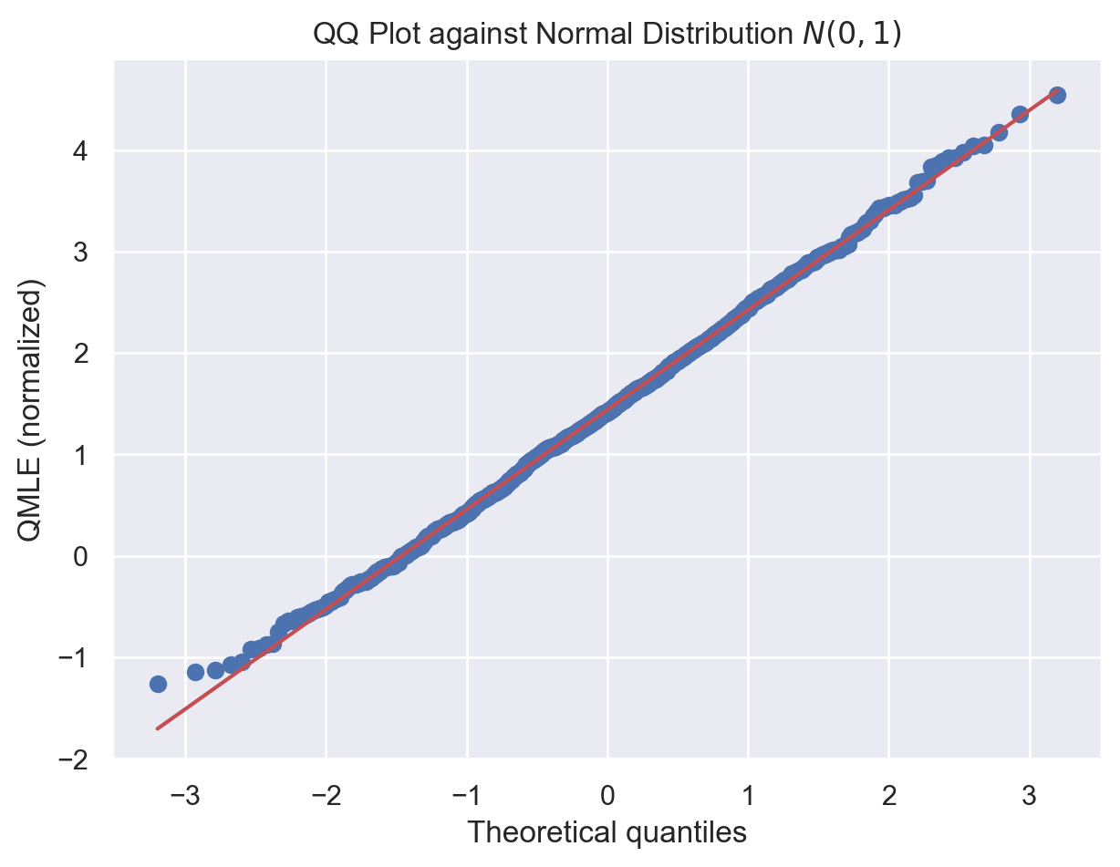
(a) QMLE

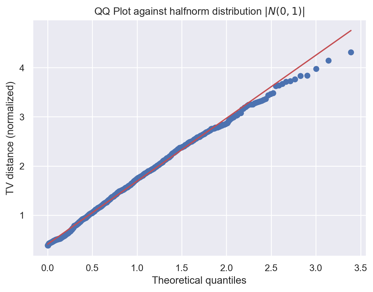
(b) TV distance

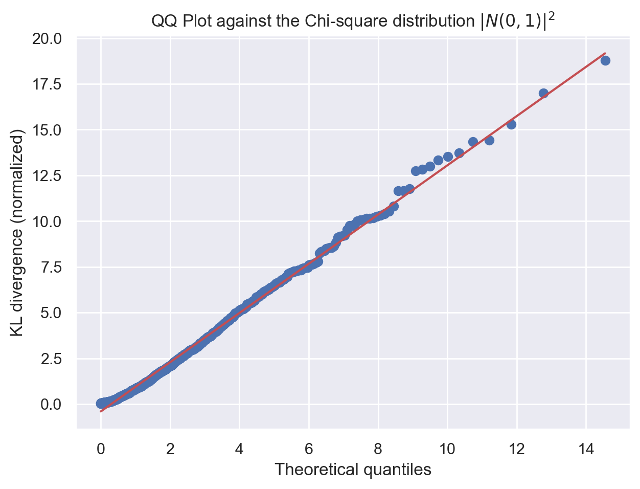
(c) KL divergence

Figure 1: QQ plots comparing empirical quantiles of normalized statistics to the corresponding theoretical distributions.

Appendix A Basic lemma

A.1 Definition of tilted measure

Let $\mu$ be the mixing distribution appearing in 1. For any $1\leq k\leq n$, define the tilted measure $\mathrm{d}\mu_{n,k}$ as

$$.1\leq\forall k\leq\forall n,\quad\mathrm{d}\mu_{n,k}(\theta)\equiv\frac{\mathrm{d}\mu(\theta)v_{n,k}(\alpha,\theta)}{\int\mathrm{d}\mu(\theta^{\prime})v_{n,k}(\alpha,\theta^{\prime})}\quad\text{with}\quad v_{n,k}(\alpha;\theta)=\frac{\prod_{i=1}^{k-1}(\theta+i\alpha)}{\prod_{i=1}^{n-1}(\theta+i)}.$$ (A.1)

Since the weight $v_{n,k}(\alpha;\theta)$ is strictly positive for all $\theta\in(-\alpha,+\infty)$, the support of the tilted probability measure $\mu_{n,k}$ is equal to the support of $\mu$. Combined with the condition on the support of $\mu$ from 1, we have

$$1\leq\forall k\leq\forall n,\quad\operatorname{supp}(\mu_{n,k})=\operatorname{supp}(\mu)\subset[\underline{\theta},\bar{\theta}]\quad\text{with}-\alpha<\underline{\theta}\leq 0\leq\bar{\theta}<+\infty.$$ (A.2)

As we will see in later, we will handle integrals of this form $\int\mathrm{d}\mu_{n,k}(\theta)h(\theta)$ for some function $h:(-\alpha,\infty)\to\mathbb{R}$ many times. By (A.2), these integrals can be estimated as

$$\inf_{\theta\in[\underline{\theta},\bar{\theta}]}h(\theta)\leq\int\mathrm{d}\mu_{n,k}(\theta)h(\theta)\leq\sup_{\theta\in[\underline{\theta},\bar{\theta}]}h(\theta)\quad\text{and}\quad\Bigl{|}\int\mathrm{d}\mu_{n,k}(\theta)h(\theta)\Bigr{|}\leq\sup_{\theta\in[\underline{\theta},\bar{\theta}]}|h(\theta)|$$ (A.3)

We will frequently use this property.

Lemma A.1 (Concentration of triangular array $v_{n,k}$).

Suppose the triangular array $v_{n,k}$ satisfies 1. Then, for any $n\in\mathbb{N}$ and $1\leq k\leq n$, we have

$$\Bigl{|}n\frac{v_{n+1,k}}{v_{n,k}}-1\Bigr{|}\vee\Bigl{|}\frac{v_{n+1,k+1}}{v_{n,k}}-\frac{k}{n}\alpha\Bigr{|}\leq\frac{\bar{\theta}-\underline{\theta}}{n+\underline{\theta}}.$$

Proof.

By 1 and the definition of tilted probability measure (A.1), we have

$$\frac{v_{n+1,k}}{v_{n,k}} =\frac{\int\mathrm{d}\mu(\theta)\frac{\prod_{i=1}^{k-1}(\theta+i\alpha)}{\prod_{i=1}^{n-1}(\theta+i)}\frac{1}{n+\theta}}{\int\mathrm{d}\mu(\theta)\frac{\prod_{i=1}^{k-1}(\theta+i\alpha)}{\prod_{i=1}^{n-1}(\theta+i)}}=\int\mathrm{d}\mu_{n,k}(\theta)\frac{1}{\theta+n}=\frac{1}{n}+{\int\mathrm{d}\mu_{n,k}(\theta)\bigl{(}\frac{1}{\theta+n}-\frac{1}{n}\bigr{)}},$$

$$\frac{v_{n+1,k+1}}{v_{n,k}} =\frac{\int\mathrm{d}\mu(\theta)\frac{\prod_{i=1}^{k-1}(\theta+i\alpha)}{\prod_{i=1}^{n-1}(\theta+i)}\frac{\theta+k\alpha}{n+\theta}}{\int\mathrm{d}\mu(\theta)\frac{\prod_{i=1}^{k-1}(\theta+i\alpha)}{\prod_{i=1}^{n-1}(\theta+i)}}=\int\mathrm{d}\mu_{n,k}(\theta)\frac{\theta+k\alpha}{\theta+n}=\frac{k}{n}\alpha+{\int\mathrm{d}\mu_{n,k}\bigl{(}\frac{\theta+k\alpha}{\theta+n}-\frac{k\alpha}{n}\bigr{)}}.$$

By the property in (A.3), it holds that

$$\Bigl{|}\frac{v_{n+1,k}}{v_{n,k}}-\frac{1}{n}\Bigr{|} \leq\sup_{\theta\in[\underline{\theta},\bar{\theta}]}|\frac{1}{\theta+n}-\frac{1}{n}|=\sup_{\theta\in[\underline{\theta},\bar{\theta}]}\Bigl{|}\frac{\theta}{n(n+\theta)}\Bigr{|}\leq\frac{1}{n}\sup_{\theta\in[\underline{\theta},\bar{\theta}]}\frac{|\theta|}{\theta+n}$$

$$\Bigl{|}\frac{v_{n+1,k+1}}{v_{n,k}}-\frac{k}{n}\alpha\Bigr{|} \leq\sup_{\theta\in[\underline{\theta},\bar{\theta}]}\Bigl{|}\frac{\theta+k\alpha}{\theta+n}-\frac{k\alpha}{n}\Bigr{|}=\sup_{\theta\in[\underline{\theta},\bar{\theta}]}\Bigl{|}\frac{(n-k\alpha)\theta}{n(\theta+n)}\Bigr{|}\leq\sup_{\theta\in[\underline{\theta},\bar{\theta}]}\frac{|\theta|}{\theta+n}$$

With $\sup_{\theta\in[\underline{\theta},\bar{\theta}]}\frac{|\theta|}{\theta+n}\leq\frac{\bar{\theta}-\underline{\theta}}{n+\underline{\theta}}$, we complete the proof. ∎

A.2 Dominated convergence theorem for empirical measure $\sum_{j=1}^{n}\frac{\mathsf{k}_{n,j}}{\mathsf{k}_{n}}\delta_{j}$

Given a partition $(U_{1},U_{2},\dots)$ of $[n]$, let $\mathsf{k}_{n,j}$ be the number of blocks of size $j$ and let $\mathsf{k}_{n}=\sum_{j=1}^{n}\mathsf{k}_{n,j}$ be the number of non-empty blocks. Since $\mathsf{k}_{n,j}=0$ for any $j\geq n+1$, this induces the following empirical measure over $\mathbb{N}$:

$$\sum_{j=1}^{\infty}\frac{\mathsf{k}_{n,j}}{\mathsf{k}_{n}}\delta_{j}.$$

By equation (1.7), this empirical measure converges to the discrete distribution $\mathfrak{p}_{\alpha}(j)$ pointwisely, i.e.,

$$\frac{\mathsf{k}_{n,j}}{\mathsf{k}_{n}}\operatorname{\;\xrightarrow{\text{a.s.}}\;}\mathfrak{p}_{\alpha}(j)=\frac{\alpha\prod_{i=1}^{j-1}(i-\alpha)}{j!}.$$

During proofs in later section, we will see many terms of the integral $\sum_{j=1}^{\infty}\frac{\mathsf{k}_{n,j}}{\mathsf{k}_{n}}f(j)$ for some function $f:\mathbb{N}\to\mathbb{R}$. The next lemma claims a dominated convergence-type theorem, i.e., if the test function $f$ is bounded, then the integral also converges almost surely.

Lemma A.2 (Dominated convergence theorem).

As $n\to+\infty$, it holds that

$$\sum_{j=1}^{\infty}\Bigl{|}\frac{\mathsf{k}_{n,j}}{\mathsf{k}_{n}}-\mathfrak{p}_{\alpha}(j)\Bigr{|}\operatorname{\;\xrightarrow{\text{a.s.}}\;}0$$

Therefore, for any bounded function $f:\mathbb{N}\to\mathbb{R}$, we have

$$\sum_{j=1}^{n}\frac{\mathsf{k}_{n,j}}{\mathsf{k}_{n}}f(j)\operatorname{\;\xrightarrow{\text{a.s.}}\;}\sum_{j=1}^{\infty}\mathfrak{p}_{\alpha}(j)f(j).$$

Proof.

This result follows from Scheffé’s Lemma applied with the point-wise convergence $\mathsf{k}_{n,j}/\mathsf{k}_{n}\operatorname{\;\xrightarrow{\text{a.s.}}\;}\mathfrak{p}_{\alpha}(j)$ (a.s.) and the fact that $(\mathsf{k}_{n,j}/\mathsf{k}_{n})_{j=1}^{\infty}$ and $(\mathfrak{p}_{\alpha}(j))_{j=1}^{\infty}$ are probability measures on $\mathbb{N}$. ∎

Appendix B $\alpha$-diversity and Fisher Information

B.1 Proof of Theorem 2.1

The proof in this section is inspired by [2], which focuses on the case $\mu=\delta_{\theta}$, and we borrow several notations from the paper. Let $\mathcal{F}_{n}$ be the $\sigma$-filed generated by the random partition of $[n]$, i.e., $(U_{1},\dots\cdots U_{\mathsf{k}_{n}})\in\mathcal{P}_{n}$. By the definition, the number of nonempty blocks $\mathsf{k}_{n}$ can be written as a summation of Bernoulli random variables as follows:

$$\mathsf{k}_{n+1}=\mathsf{k}_{n}+\xi_{n+1},\quad\xi_{n+1}|\mathcal{F}_{n}\sim\operatorname{Bernoulli}(p_{n}),\quad p_{n}\equiv\frac{v_{n+1,\mathsf{k}_{n}+1}}{v_{n,\mathsf{k}_{n}}}.$$

By 1, the success probability $p_{n}$ can be expressed as an integral of tilted measure:

$$p_{n}=\frac{\int\mathrm{d}\mu(\theta)v_{n,\mathsf{k}_{n}}(\alpha,\theta)\frac{\theta+\mathsf{k}_{n}\alpha}{\theta+n}}{\int\mathrm{d}\mu(\theta)v_{n,\mathsf{k}_{n}}(\alpha,\theta)}=\int\mathrm{d}\mu_{n,\mathsf{k}_{n}}(\theta)\frac{\theta+\mathsf{k}_{n}\alpha}{\theta+n}.$$

Here $\mathrm{d}\mu_{n,\mathsf{k}_{n}}$ is the tilted probability measure (A.1) with $k=\mathsf{k}_{n}$. Here, the integrand $(\theta+\mathsf{k}_{n}\alpha)/(\theta+n)$ is increasing in $\theta\in(-\alpha,+\infty)$ by $\alpha\mathsf{k}_{n}<1\cdot n$. Thus, using the property of (A.3), we get

$$\underline{p}_{n}\equiv\frac{\underline{\theta}+\alpha\mathsf{k}_{n}}{\underline{\theta}+n}\leq p_{n}\leq\frac{\bar{\theta}+\alpha\mathsf{k}_{n}}{\bar{\theta}+n}=:\bar{p}_{n}$$ (B.1)

Then, using the estimate $p_{n}\leq\bar{p}_{n}$, the conditional expectation $\operatorname{\mathbb{E}}[\mathsf{k}_{n+1}|\mathcal{F}_{n}]$ is bounded from above as

$$\operatorname{\mathbb{E}}[\mathsf{k}_{n+1}|\mathcal{F}_{n}] =\mathsf{k}_{n}+p_{n} \mathsf{k}_{n+1}=\mathsf{k}_{n}+\xi_{n+1},\ \xi_{n+1}|\mathcal{F}_{n}\sim\operatorname{Bernoulli}(p_{n})$$

$$\leq\mathsf{k}_{n}+\frac{\bar{\theta}+\mathsf{k}_{n}\alpha}{\bar{\theta}+n} p_{n}\leq\bar{p}_{n}=\frac{\bar{\theta}+\alpha\mathsf{k}_{n}}{\bar{\theta}+n}.$$

Rearranging the above display, we get

$$\operatorname{\mathbb{E}}\Bigl{[}\mathsf{k}_{n+1}+\frac{\bar{\theta}}{\alpha}\mid\mathcal{F}_{n}\Bigr{]} \leq\Bigl{(}\mathsf{k}_{n}+\frac{\bar{\theta}}{\alpha}\Bigr{)}\Bigl{(}1+\frac{\alpha}{\bar{\theta}+n}\Bigr{)}.$$

This means that $\bar{M}_{n}$ defined by

$$\bar{M}_{n}\equiv\bar{b}_{n}(\mathsf{k}_{n}+\frac{\bar{\theta}}{\alpha})\quad\text{with}\quad\bar{b}_{n}\equiv\prod_{k=1}^{n-1}\Bigl{(}1+\frac{\alpha}{\bar{\theta}+k}\Bigr{)}^{-1}=\prod_{k=1}^{n-1}\Bigl{(}\frac{\bar{\theta}+k}{\bar{\theta}+k+\alpha}\Bigr{)}$$ (B.2)

is a non-negative super martingale, i.e.,

$$\bar{M}_{n}\geq 0,\quad\operatorname{\mathbb{E}}[\bar{M}_{n+1}|\mathcal{F}_{n}]\leq\bar{M}_{n}.$$

Then, by Doob’s martingale convergence theorem (cf. [13, Theorem 4.2.12]), there exists a positive random variable $\bar{M}_{\infty}$ such that

$$\bar{M}_{n}\operatorname{\;\xrightarrow{\text{a.s.}}\;}\bar{M}_{\infty},\quad\bar{M}_{\infty}\in L_{1}.$$

With $\Gamma(n+\alpha)/\Gamma(n)\sim n^{\alpha}$ for any $\alpha\in\mathbb{R}$, the coefficient $\bar{b}_{n}$ appearing in (B.2) behave asymptotically as

$$\bar{b}_{n}=\frac{\Gamma(\bar{\theta}+\alpha+1)}{\Gamma(\bar{\theta}+1)}\frac{\Gamma(\bar{\theta}+n)}{\Gamma(\bar{\theta}+\alpha+n)}\sim n^{-\alpha}\frac{\Gamma(\bar{\theta}+\alpha+1)}{\Gamma(\bar{\theta}+1)}.$$ (B.3)

Combined with the definition $\bar{M}_{n}=\bar{b}_{n}(\mathsf{k}_{n}+\bar{\theta}/\alpha)$ and $\bar{M}_{n}\operatorname{\;\xrightarrow{\text{a.s.}}\;}\bar{M}_{\infty}\in L_{1}$, we get

$$n^{-\alpha}\mathsf{k}_{n}\operatorname{\;\xrightarrow{\text{a.s.}}\;}\mathsf{S}_{\alpha,\mu}\equiv\frac{\Gamma(\bar{\theta}+1)}{\Gamma(\bar{\theta}+\alpha+1)}\bar{M}_{\infty}\in L_{1}.$$ (B.4)

Furthermore, since $\bar{M}_{n}$ is a super martingale with $\bar{M}_{1}=1+\frac{\bar{\theta}}{\alpha}$, it holds that

$$b_{n}\operatorname{\mathbb{E}}[\mathsf{k}_{n}+\frac{\bar{\theta}}{\alpha}]=\operatorname{\mathbb{E}}[\bar{M}_{n}]\leq\operatorname{\mathbb{E}}[\bar{M}_{1}]=1+\frac{\bar{\theta}}{\alpha}.$$

Combined with (B.3), we obtain the upper bound of $\operatorname{\mathbb{E}}[\mathsf{k}_{n}]$:

$$\operatorname{\mathbb{E}}[\mathsf{k}_{n}] \leq\bar{b}_{n}^{-1}\Bigl{(}1+\frac{\bar{\theta}}{\alpha}\Bigr{)}-\frac{\bar{\theta}}{\alpha}\sim n^{\alpha}\frac{\Gamma(\bar{\theta}+1)}{\Gamma(\bar{\theta}+\alpha+1)}\Bigl{(}1+\frac{\bar{\theta}}{\alpha}\Bigr{)}=n^{\alpha}\frac{\Gamma(\bar{\theta}+1)}{\alpha\Gamma(\bar{\theta}+\alpha)}.$$ (B.5)

Next, we will show $n^{-\alpha}\mathsf{k}_{n}\to\mathsf{S}_{\alpha,\mu}$ in $L^{2}$ (stronger than (B.4)) by constructing a sub-martingale and applying Doob’s maximum $L_{p}$ inequality. Now, similarly to (B.2), we define $\underline{M}_{n}$ as

$$\underline{M}_{n}=\underline{b}_{n}(\mathsf{k}_{n}+\frac{\underline{\theta}}{\alpha}),\quad\underline{b}_{n}\equiv\prod_{k=1}^{n-1}\Bigl{(}\frac{\underline{\theta}+k}{\underline{\theta}+k+\alpha}\Bigr{)}=\frac{\Gamma(\underline{\theta}+\alpha+1)}{\Gamma(\underline{\theta}+1)}\frac{\Gamma(\underline{\theta}+n)}{\Gamma(\underline{\theta}+\alpha+n)}$$

Then, by the same argument for $\bar{M}_{n}$, now using the lower estimate $\underline{p}_{n}\leq p_{n}$ in (B.1), one can show that $\underline{M}_{n}$ is non-negative sub martingale, i.e.,

$$\underline{M}_{n}\geq 0,\quad\operatorname{\mathbb{E}}[\underline{M}_{n+1}|\mathcal{F}_{n}]\geq\underline{M}_{n}.$$

Furthermore, by the same argument for $\bar{b}_{n}$ in (B.3), the leading term of $\underline{b}_{n}$ is given by

$$\underline{b}_{n}\sim n^{-\alpha}\frac{\Gamma(\underline{\theta}+\alpha+1)}{\Gamma(\underline{\theta}+1)}.$$ (B.6)

By the same argument in (B.5), now using the sub-martingale property of $\bar{M}_{n}$, we also get the lower bound of $\operatorname{\mathbb{E}}[\mathsf{k}_{n}]$:

$$\operatorname{\mathbb{E}}[\mathsf{k}_{n}] \gtrsim n^{\alpha}\frac{\Gamma(\underline{\theta}+1)}{\alpha\Gamma(\underline{\theta}+\alpha)}.$$ (B.7)

Combining (B.4), (B.6), and $\underline{M}_{n}=\underline{b}_{n}(\mathsf{k}_{n}+\frac{\underline{\theta}}{\alpha})$, we obtain

$$\underline{M}_{n}\sim\frac{\Gamma(\underline{\theta}+\alpha+1)}{\Gamma(\underline{\theta}+1)}n^{-\alpha}\Bigl{(}\mathsf{k}_{n}+\frac{\underline{\theta}}{\alpha}\Bigr{)}\operatorname{\;\xrightarrow{\text{a.s.}}\;}\underline{M}_{\infty}\equiv\frac{\Gamma(\underline{\theta}+\alpha+1)}{\Gamma(\underline{\theta}+1)}\mathsf{S}_{\alpha,\mu}\in L_{1}.$$

Next, we will show that the non-negative sub martingale $\underline{M}_{n}$ is bounded in $L_{2}$, i.e., $\sup_{n\geq 1}\|\underline{M}_{n}\|_{2}<+\infty$. Note that the increment of $\bar{M}_{n}$ can be written as

$$\underline{M}_{n+1}-\underline{M}_{n} =\underline{b}_{n+1}(\mathsf{k}_{n+1}+\frac{\underline{\theta}}{\alpha})-\underline{b}_{n}(K_{n}+\frac{\underline{\theta}}{\alpha})$$

$$=\underline{b}_{n+1}(K_{n}+\xi_{n+1}+\frac{\underline{\theta}}{\alpha})-\underline{b}_{n}(K_{n}+\frac{\underline{\theta}}{\alpha})$$

$$=\underline{b}_{n+1}\Bigl{(}\xi_{n+1}-(\frac{\underline{b}_{n}}{\underline{b}_{n+1}}-1)(\mathsf{k}_{n}+\frac{\underline{\theta}}{\alpha})\Bigr{)}$$

$$=\underline{b}_{n+1}\Bigl{(}\xi_{n+1}-\frac{\alpha}{n+\underline{\theta}}(\mathsf{k}_{n}+\frac{\underline{\theta}}{\alpha})\Bigr{)} \underline{b}_{n}=\prod_{k=1}^{n-1}\Bigl{(}\frac{\underline{\theta}+k}{\underline{\theta}+k+\alpha}\Bigr{)}$$

$$=\underline{b}_{n+1}\Bigl{(}\xi_{n+1}-\underline{p}_{n}\Bigr{)} \underline{p}=\frac{\alpha\mathsf{k}_{n}+\underline{\theta}}{n+\underline{\theta}}.$$

Then, we have

$$\operatorname{\mathbb{E}}[(\underline{M}_{n}-\underline{M}_{1})^{2}] =\operatorname{\mathbb{E}}\Bigl{[}\Bigl{(}\sum_{i=1}^{n-1}(\underline{M}_{i+1}-\underline{M}_{i})\Bigr{)}^{2}\Bigr{]}$$

$$=\sum_{k=1}^{n-1}\underline{b}_{k+1}^{2}\operatorname{\mathbb{E}}[(\xi_{k+1}-\underline{p}_{k})^{2}]+2\sum_{1\leq k<\ell\leq n-1}\underline{b}_{k+1}\underline{b}_{\ell+1}\operatorname{\mathbb{E}}\bigl{[}(\xi_{k+1}-\underline{p}_{k})(\xi_{\ell+1}-\underline{p}_{\ell})\bigr{]}$$ (B.8)

Now we claim $\sup_{n\geq 1}\operatorname{\mathbb{E}}[(M_{n}-M_{1})^{2}]<+\infty$. First, let us derive an upper bound of the first term. By the tower property, as $k\to+\infty$,

$$\operatorname{\mathbb{E}}[(\xi_{k+1}-\underline{p}_{k})^{2}] =\operatorname{\mathbb{E}}[\operatorname{\mathbb{E}}[(\xi_{k+1}-\underline{p}_{k})^{2}|\mathcal{F}_{k}]]$$

$$=\operatorname{\mathbb{E}}[p_{k}(1-\underline{p}_{k})^{2}+(1-p_{k})\underline{p}_{k}^{2}] \xi_{k+1}|\mathcal{F}_{k}\sim\operatorname{Bernoulli}(p_{k})$$

$$\leq 2\operatorname{\mathbb{E}}[\bar{p}_{k}] 0\leq\underline{p}_{k}\leq p_{k}\leq\bar{p}_{k}\leq 1$$

$$=2\frac{\bar{\theta}+\alpha\operatorname{\mathbb{E}}[\mathsf{k}_{k}]}{k+\bar{\theta}}$$

$$\lesssim k^{-1+\alpha} \operatorname{\mathbb{E}}[\mathsf{k}_{n}]\lesssim n^{\alpha}$$ from (B.5)

Combined with $\underline{b}_{n}\asymp n^{-\alpha}$ from (B.6), we have that, as $n\to+\infty$,

$$\sum_{k=1}^{n-1}\underline{b}_{k+1}^{2}\operatorname{\mathbb{E}}\bigl{[}(\xi_{k+1}-\underline{p}_{k})^{2}\bigr{]}\lesssim\sum_{k=1}^{n-1}k^{-2\alpha}k^{-1+\alpha}=\sum_{k=1}^{n-1}k^{-(1+\alpha)}=O(1).$$ (B.9)

Next, let us bound the cross term $\underline{b}_{k+1}\underline{b}_{\ell+1}\operatorname{\mathbb{E}}[(\xi_{k+1}-\underline{p}_{k})(\xi_{\ell+1}-\underline{p}_{\ell})]$. By $\underline{p}_{n}\leq p_{n}\leq\bar{p}_{n}$ and $\operatorname{\mathbb{E}}[\xi_{n+1}|\mathcal{F}_{n}]=p_{n}$,

$$\operatorname{\mathbb{E}}[\xi_{n+1}-\underline{p}_{n}|\mathcal{F}_{n}]=\operatorname{\mathbb{E}}[p_{n}-\underline{p}_{n}]\geq 0$$

and

$$p_{n}-\underline{p}_{n} \leq\bar{p}_{n}-\underline{p}_{n}$$

$$=\frac{\bar{\theta}+\alpha\mathsf{k}_{n}}{\bar{\theta}+n}-\frac{\underline{\theta}+\alpha\mathsf{k}_{n}}{\underline{\theta}+n}$$

$$=\frac{\bar{\theta}-\underline{\theta}}{(\bar{\theta}+n)(\underline{\theta}+n)}(n-\alpha\mathsf{k}_{n})$$

$$\leq\frac{\bar{\theta}-\underline{\theta}}{(\underline{\theta}+n)} 0\leq\alpha\mathsf{k}_{n}<n,\ \bar{\theta}\geq 0$$

for all $n$. Let us fix $k<\ell$. With $k+1\leq\ell$, using the tower property,

$$\operatorname{\mathbb{E}}\bigl{[}(\xi_{k+1}-\underline{p}_{k})(\xi_{\ell+1}-\underline{p}_{\ell})|\mathcal{F}_{k+1}\bigr{]} =(\xi_{k+1}-\underline{p}_{k})\operatorname{\mathbb{E}}\Bigl{[}(\xi_{\ell+1}-\underline{p}_{\ell})|\mathcal{F}_{k+1}\Bigr{]}$$

$$=(\xi_{k+1}-\underline{p}_{k})\operatorname{\mathbb{E}}\Bigl{[}\operatorname{\mathbb{E}}\bigl{[}(\xi_{\ell+1}-\underline{p}_{\ell})|\mathcal{F}_{\ell}\bigr{]}|\mathcal{F}_{k+1}\Bigr{]}$$

$$=(\xi_{k+1}-\underline{p}_{k})\operatorname{\mathbb{E}}\bigl{[}(p_{\ell}-\underline{p}_{\ell})|\mathcal{F}_{k+1}\bigr{]}$$

so

$$\Bigl{|}\operatorname{\mathbb{E}}\bigl{[}(\xi_{k+1}-\underline{p}_{k})(\xi_{\ell+1}-\underline{p}_{\ell})|\mathcal{F}_{k+1}\bigr{]}\Bigr{|} \leq\bigl{|}\xi_{k+1}-\underline{p}_{k}\bigr{|}\operatorname{\mathbb{E}}\bigl{[}|p_{\ell}-\underline{p}_{\ell}|\mid\mathcal{F}_{k+1}\bigr{]}\leq\bigl{|}\xi_{k+1}-\underline{p}_{k}\bigr{|}\frac{\bar{\theta}-\underline{\theta}}{\underline{\theta}+\ell}$$

This gives

$$\left|\operatorname{\mathbb{E}}\bigl{[}(\xi_{k+1}-\underline{p}_{k})(\xi_{\ell+1}-\underline{p}_{\ell})\bigr{]}\right| =\left|\operatorname{\mathbb{E}}\Bigl{[}\operatorname{\mathbb{E}}\bigl{[}(\xi_{k+1}-\underline{p}_{k})(\xi_{\ell+1}-\underline{p}_{\ell})|\mathcal{F}_{k+1}\bigr{]}\Bigr{]}\right|$$

$$\leq\operatorname{\mathbb{E}}\Bigl{[}\Bigl{|}\operatorname{\mathbb{E}}[(\xi_{k+1}-\underline{p}_{k})(\xi_{\ell+1}-\underline{p}_{\ell})|\mathcal{F}_{k+1}]\Bigr{|}\Bigr{]}$$

$$\leq\operatorname{\mathbb{E}}[|\xi_{k+1}-\underline{p}_{k}|]\cdot\frac{\bar{\theta}-\underline{\theta}}{\underline{\theta}+\ell}$$

where

$$\operatorname{\mathbb{E}}[|\xi_{k+1}-\underline{p}_{k}|] =\operatorname{\mathbb{E}}[\operatorname{\mathbb{E}}[|\xi_{k+1}-\underline{p}_{k}|\mid\mathcal{F}_{k}]]$$

$$=\operatorname{\mathbb{E}}[p_{k}(1-\underline{p}_{k})+(1-p_{k})\underline{p}_{k}]$$

$$\leq 2\operatorname{\mathbb{E}}[\underline{p}_{k}]$$

$$=2\frac{\bar{\theta}+\alpha\operatorname{\mathbb{E}}[\mathsf{k}_{k}]}{k+\bar{\theta}}.$$

Therefore, the cross term is upper bounded as

$$\left|\sum_{1\leq k<\ell\leq n-1}\underline{b}_{k+1}\underline{b}_{\ell+1}\operatorname{\mathbb{E}}[(\xi_{k+1}-\underline{p}_{k})(\xi_{\ell+1}-\underline{p}_{\ell})]\right| \leq\sum_{1\leq k<\ell\leq n-1}\underline{b}_{k+1}\underline{b}_{\ell+1}\Bigl{|}\operatorname{\mathbb{E}}[(\xi_{k+1}-\underline{p}_{k})(\xi_{\ell+1}-\underline{p}_{\ell})]\Bigr{|}$$

$$\leq\sum_{1\leq k<\ell\leq n-1}\underline{b}_{k+1}\underline{b}_{\ell+1}\frac{\bar{\theta}-\underline{\theta}}{\underline{\theta}+\ell}\cdot 2\frac{\bar{\theta}+\alpha\operatorname{\mathbb{E}}[\mathsf{k}_{k}]}{k+\bar{\theta}}$$

$$=\sum_{\ell=2}^{n-1}\underline{b}_{\ell+1}\frac{\bar{\theta}-\underline{\theta}}{\ell+\underline{\theta}}\cdot\sum_{k=1}^{\ell-1}2\underline{b}_{k+1}\cdot\frac{\bar{\theta}+\alpha\operatorname{\mathbb{E}}[\mathsf{k}_{k}]}{k+\bar{\theta}}$$

Here, as $k\to+\infty$, using $\underline{b}_{k}\asymp k^{-\alpha}$ and $\operatorname{\mathbb{E}}[\mathsf{k}_{k}]\lesssim k^{\alpha}$

$$\underline{b}_{k+1}\cdot\frac{\bar{\theta}+\alpha\operatorname{\mathbb{E}}[\mathsf{k}_{k}]}{k+\bar{\theta}}\lesssim k^{-\alpha}\frac{k^{\alpha}}{k}=\frac{1}{k},$$

so that as $\ell\to+\infty$,

$$\sum_{k=1}^{\ell-1}2\underline{b}_{k+1}\cdot\frac{\bar{\theta}+\alpha\operatorname{\mathbb{E}}[\mathsf{k}_{k}]}{k+\bar{\theta}}\lesssim\log\ell.$$

This in turn gives

$$\underline{b}_{\ell+1}\frac{\bar{\theta}-\underline{\theta}}{\ell+\underline{\theta}}\cdot\sum_{k=1}^{\ell-1}2\underline{b}_{k+1}\cdot\frac{\bar{\theta}+\alpha\operatorname{\mathbb{E}}[\mathsf{k}_{k}]}{k+\bar{\theta}}\lesssim\ell^{-\alpha}\frac{1}{\ell}\log\ell=\frac{\log\ell}{\ell^{\alpha+1}}$$

as $\ell\to+\infty$. Therefore, we have that, as $n\to+\infty$,

$$\Bigl{|}\sum_{1\leq k<\ell\leq n-1}\underline{b}_{k+1}\underline{b}_{\ell+1}\operatorname{\mathbb{E}}[(\xi_{k+1}-\underline{p}_{k})(\xi_{\ell+1}-\underline{p}_{\ell})]\Bigr{|}\lesssim\sum_{\ell=2}^{n-1}\frac{\log\ell}{\ell^{\alpha+1}}=O(1)$$ (B.10)

where we have used the fact that $\int_{1}^{\infty}x^{-(\alpha+1)}\log x$ is finite.

Putting (B.8), (B.9), and (B.10) together, we obtain

$$\sup_{n\geq 1}\operatorname{\mathbb{E}}[(\underline{M}_{n}-\underline{M}_{1})^{2}]<+\infty.$$

With $\underline{M}_{1}=1+\frac{\underline{\theta}}{\alpha}$, which is a deterministic constant, we conclude that $\underline{M}_{n}$ is bounded in $L_{2}$. Since $\underline{M}_{n}$ is non-negative sub martingale, Doob’s maximum $L_{p}$ inequality with $p=2$ (cf. [13, Theorem 4.4.4]) yields

$$\operatorname{\mathbb{E}}\Bigl{[}\bigl{(}\sup_{n\geq 1}|\underline{M}_{n}|\bigr{)}^{2}\Bigr{]}\leq\Bigl{(}\frac{2}{2-1}\Bigr{)}^{2}\sup_{n\geq 1}\operatorname{\mathbb{E}}[|\underline{M}_{n}|^{2}]<+\infty$$

On the other hand, since $\underline{M}_{n}$ converges to $\underline{M}_{\infty}$ almost surely as $n\to+\infty$, we have

$$\sup_{n\geq 1}|\underline{M}_{n}-\underline{M}_{\infty}|^{2}\leq\bigl{(}2\sup_{n\geq 1}|\underline{M}_{n}|\bigr{)}^{2}.$$

Therefore, the dominated convergence theorem gives

$$\lim_{n\to+\infty}\operatorname{\mathbb{E}}[|\underline{M}_{n}-\underline{M}_{\infty}|^{2}]=\operatorname{\mathbb{E}}[\lim_{n\to+\infty}|\underline{M}_{n}-\underline{M}_{\infty}|^{2}]=0.$$

This concludes that $\underline{M}_{n}$ converges to $\underline{M}_{\infty}$ in $L_{2}$. Moreover, since $\underline{M}_{n}$ is bounded in $L_{2}$, we also get $\underline{M}_{\infty}\in L_{2}$. Finally, combining

$$\underline{M}_{n}=\underline{b}_{n}(\mathsf{k}_{n}+\frac{\underline{\theta}}{\alpha}),\quad\underline{b}_{n}\sim n^{-\alpha}\frac{\Gamma(\underline{\theta}+\alpha+1)}{\Gamma(\underline{\theta}+1)},\quad\underline{M}_{\infty}=\frac{\Gamma(\underline{\theta}+\alpha+1)}{\Gamma(\underline{\theta}+1)}\mathsf{S}_{\alpha,\mu},$$

and noting that $\underline{b}_{n}$ is deterministic, we conclude that $\mathsf{S}_{\alpha,\mu}\in L_{2}$ and $n^{-\alpha}\mathsf{k}_{n}\to^{L^{2}}\mathsf{S}_{\alpha,\mu}$.

The inequality (2.1) of $\operatorname{\mathbb{E}}[\mathsf{S}_{\alpha,\mu}]$ immediately follows from (B.5), (B.7), and the $L_{1}$ convergence $n^{-\alpha}\mathsf{k}_{n}\to^{L^{1}}\mathsf{S}_{\alpha,\mu}$.

B.2 Proof of Theorem 2.3

Let $\ell_{n}(\alpha;\mu)$ be the log-likelihood given by (2.2). Since the marginal distribution of the Gibbs partition is a discrete distribution over $\mathcal{P}_{n}$, the expectation $\operatorname{\mathbb{E}}$ over the law and derivative with respect to $\alpha$ is interchangeable. As a result, it holds that

$$\operatorname{\mathbb{E}}[(\partial_{\alpha}\ell_{n}(\alpha;\mu)^{2})]=-\operatorname{\mathbb{E}}[\partial_{\alpha}^{2}\ell_{n}(\alpha;\mu)],$$

and hence it suffices to show $n^{-\alpha}\operatorname{\mathbb{E}}[\partial_{\alpha}^{2}\ell_{n}(\alpha;\mu)]\to-\operatorname{\mathbb{E}}[\mathsf{S}_{\alpha,\mu}]\mathfrak{i}(\alpha)$.

Here, the first and the second derivative of the log-likelihood function are given by

$$\partial_{\alpha}\ell_{n}(\alpha;\mu) =\frac{\partial}{\partial\alpha}\left(\log\Bigl{(}\int\mathrm{d}\mu(\theta)\frac{\prod_{i=1}^{\mathsf{k}_{n}-1}(\theta+i\alpha)}{\prod_{i=1}^{n-1}(\theta+i)}\Bigr{)}+\sum_{j=2}^{n}\mathsf{k}_{n,j}\sum_{i=1}^{j-1}\log(i-\alpha)\right)$$

$$=\frac{\frac{\partial}{\partial\alpha}\int\mathrm{d}\mu(\theta)\frac{\prod_{i=1}^{\mathsf{k}_{n}-1}(\theta+i\alpha)}{\prod_{i=1}^{n-1}(\theta+i)}}{\int\mathrm{d}\mu(\theta)\frac{\prod_{i=1}^{\mathsf{k}_{n}-1}(\theta+i\alpha)}{\prod_{i=1}^{n-1}(\theta+i)}}-\sum_{j=2}^{n}\mathsf{k}_{n,j}\sum_{i=1}^{j-1}\frac{1}{i-\alpha},$$

$$\partial_{\alpha}^{2}\ell_{n}(\alpha;\mu) =\frac{\frac{\partial^{2}}{\partial\alpha^{2}}\int\mathrm{d}\mu(\theta)\frac{\prod_{i=1}^{\mathsf{k}_{n}-1}(\theta+i\alpha)}{\prod_{i=1}^{n-1}(\theta+i)}}{\int\mathrm{d}\mu(\theta)\frac{\prod_{i=1}^{\mathsf{k}_{n}-1}(\theta+i\alpha)}{\prod_{i=1}^{n-1}(\theta+i)}}-\left(\frac{\frac{\partial}{\partial\alpha}\int\mathrm{d}\mu(\theta)\frac{\prod_{i=1}^{\mathsf{k}_{n}-1}(\theta+i\alpha)}{\prod_{i=1}^{n-1}(\theta+i)}}{\int\mathrm{d}\mu(\theta)\frac{\prod_{i=1}^{\mathsf{k}_{n}-1}(\theta+i\alpha)}{\prod_{i=1}^{n-1}(\theta+i)}}\right)^{2}-\sum_{j=1}^{n}\mathsf{k}_{n,j}\sum_{i=1}^{j-1}\frac{1}{(i-\alpha)^{2}},$$

Now we claim that the derivative $\partial_{\alpha},\partial_{\alpha}^{2}$ and the integration $\int\mathrm{d}\mu$ appearing above are interchangeable. This is because the first and second derivative of the integrand $\frac{\prod_{i=1}^{\mathsf{k}_{n}-1}(\theta+i\alpha)}{\prod_{i=1}^{n-1}(\theta+i)}$ with respect to $\alpha$ are given by

$$\frac{\partial}{\partial\alpha}\Bigl{(}\frac{\prod_{i=1}^{\mathsf{k}_{n}-1}(\theta+i\alpha)}{\prod_{i=1}^{n-1}(\theta+i)}\Bigr{)} =\frac{\prod_{i=1}^{\mathsf{k}_{n}-1}(\theta+i\alpha)}{\prod_{i=1}^{n-1}(\theta+i)}\sum_{i=1}^{\mathsf{k}_{n}-1}\frac{i}{\theta+i\alpha}$$

$$\frac{\partial^{2}}{\partial\alpha^{2}}\Bigl{(}\frac{\prod_{i=1}^{\mathsf{k}_{n}-1}(\theta+i\alpha)}{\prod_{i=1}^{n-1}(\theta+i)}\Bigr{)} =\frac{\prod_{i=1}^{\mathsf{k}_{n}-1}(\theta+i\alpha)}{\prod_{i=1}^{n-1}(\theta+i)}\Bigl{(}\sum_{i=1}^{\mathsf{k}_{n}-1}\frac{i}{\theta+i\alpha}\Bigr{)}^{2}-\frac{\prod_{i=1}^{\mathsf{k}_{n}-1}(\theta+i\alpha)}{\prod_{i=1}^{n-1}(\theta+i)}\sum_{i=1}^{\mathsf{k}_{n}-1}\frac{i^{2}}{(\theta+i\alpha)^{2}}.$$

By 1 the support of $\mu$ is contained in $[\underline{\theta},\bar{\theta}]$ with $-\alpha<\underline{\theta}<\bar{\theta}<+\infty$, while the second derivative above is continuous in $\theta$ over the support $[\underline{\theta},\bar{\theta}]$. Therefore, the derivative $\partial_{\alpha},\partial_{\alpha}^{2}$ and the integration $\int\mathrm{d}\mu$ are interchangeable.

Substituting the derivative formula of $\partial_{\alpha}^{2}$ to the previous display of $\partial_{\alpha}^{2}\ell_{n}(\alpha;\mu)$, changing the order of $\partial_{\alpha}^{2}$ and $\int\mathrm{d}\mu$, using the definition of tilted measure $\mathrm{d}\mu_{n,\mathsf{k}_{n}}$, we get

$$\partial_{\alpha}^{2}\ell_{n}(\alpha;\mu)$$

$$=\int\mathrm{d}\mu_{n,\mathsf{k}_{n}}(\theta)\Bigl{(}\sum_{i=1}^{\mathsf{k}_{n}-1}\frac{i}{\theta+i\alpha}\Bigr{)}^{2}-\int\mathrm{d}\mu_{n,\mathsf{k}_{n}}(\theta)\sum_{i=1}^{\mathsf{k}_{n}-1}\frac{i^{2}}{(\theta+i\alpha)^{2}}-\Bigl{(}\int\mathrm{d}\mu_{n,\mathsf{k}_{n}}(\theta)\sum_{i=1}^{\mathsf{k}_{n}-1}\frac{i}{\theta+i\alpha}\Bigr{)}^{2}-\sum_{j=1}^{n}\mathsf{k}_{n,j}\sum_{i=1}^{j-1}\frac{1}{(i-\alpha)^{2}}$$

$$=\mathcal{V}_{\theta\sim\mu_{n,\mathsf{k}_{n}}}\Bigl{[}\sum_{i=1}^{\mathsf{k}_{n}-1}\frac{i}{\theta+i\alpha}\Bigr{]}-\mathcal{E}_{\theta\sim\mu_{n,\mathsf{k}_{n}}}\Bigl{[}\sum_{i=1}^{\mathsf{k}_{n}-1}\frac{i^{2}}{(\theta+i\alpha)^{2}}\Bigr{]}-\sum_{j=1}^{n}\mathsf{k}_{n,j}\sum_{i=1}^{j-1}\frac{1}{(i-\alpha)^{2}},$$

where we have defined the integral operator $\mathcal{E}$ and variance operator $\mathcal{V}$ under $\mu_{n,\mathsf{k}_{n}}$ as follows:

$$\mathcal{E}_{\theta\sim\mu_{n,\mathsf{k}_{n}}}[f(\theta)]\equiv\int\mathrm{d}\mu_{n}(\theta)f(\theta),\quad\mathcal{V}_{\theta\sim\mu_{n,\mathsf{k}_{n}}}[f(\theta)]\equiv\mathcal{E}_{\theta\sim\mu_{n,\mathsf{k}_{n}}}[f(\theta)^{2}]-\Bigl{(}\mathcal{E}_{\theta\sim\mu_{n,\mathsf{k}_{n}}}[f(\theta)]\Bigr{)}^{2}.$$

In particular, if we take the Dirac measure $\mu=\delta_{0}$, noting that $\mu_{n,\mathsf{k}_{n}}=\delta_{0}$, we get

$$\partial_{\alpha}^{2}\ell_{n}(\alpha;\delta_{0})=0-\frac{\mathsf{k}_{n}-1}{\alpha^{2}}-\sum_{j=1}^{n}\mathsf{k}_{n,j}\sum_{i=1}^{j-1}\frac{1}{(i-\alpha)^{2}}.$$ (B.11)

Taking the difference between $\partial_{\alpha}^{2}\ell_{n}(\alpha;\delta_{0})$ and $\partial_{\alpha}^{2}\ell_{n}(\alpha;\mu)$, we have

$$-\partial_{\alpha}^{2}\ell_{n}(\alpha;\mu)+\partial_{\alpha}^{2}\ell_{n}(\alpha;\delta_{0})=-\mathcal{V}_{\theta\sim\mu_{n,\mathsf{k}_{n}}}\Bigl{[}\sum_{i=1}^{\mathsf{k}_{n}-1}\frac{i}{\theta+i\alpha}\Bigr{]}+\mathcal{E}_{\theta\sim\mu_{n,\mathsf{k}_{n}}}\Bigl{[}\sum_{i=1}^{\mathsf{k}_{n}-1}\Bigl{(}\frac{i^{2}}{(\theta+i\alpha)^{2}}-\frac{1}{\alpha^{2}}\Bigr{)}\Bigr{]}.$$

Let us bound the variance term. Since the integrand can be decomposed as

$$\sum_{i=1}^{\mathsf{k}_{n}-1}\frac{i}{\theta+i\alpha}=\frac{1}{\alpha}-\sum_{i=1}^{\mathsf{k}_{n}-1}\frac{\theta}{\alpha(\theta+i\alpha)},$$

where $1/\alpha$ is constant (with respect to $\theta\sim\mu_{n,\mathsf{k}_{n}}$), we have

$$0\leq\mathcal{V}_{\theta}\Bigl{(}\sum_{i=1}^{\mathsf{k}_{n}-1}\frac{i}{\theta+i\alpha}\Bigr{)} =\mathcal{V}_{\theta}\Bigl{(}\sum_{i=1}^{\mathsf{k}_{n}-1}\frac{\theta}{\alpha(\theta+i\alpha)}\Bigr{)}\leq\mathcal{E}_{\theta\sim\mu_{n,\mathsf{k}_{n}}}\Bigl{[}\Bigl{(}\sum_{i=1}^{\mathsf{k}_{n}-1}\frac{\theta}{\alpha(\theta+i\alpha)}\Bigr{)}^{2}\Bigr{]}$$

This leads to

$$\bigl{|}\partial_{\alpha}^{2}\ell_{n}(\alpha;\mu)-\partial_{\alpha}^{2}\ell_{n}(\alpha;\delta_{0})\bigr{|}\leq\mathcal{E}_{\theta\sim\mu_{n,\mathsf{k}_{n}}}\Bigl{[}\Bigl{(}\sum_{i=1}^{\mathsf{k}_{n}-1}\frac{\theta}{\alpha(\theta+i\alpha)}\Bigr{)}^{2}\Bigr{]}+\mathcal{E}_{\theta\sim\mu_{n,\mathsf{k}_{n}}}\Bigl{[}\Bigl{|}\sum_{i=1}^{\mathsf{k}_{n}-1}\Bigl{(}\frac{i^{2}}{(\theta+i\alpha)^{2}}-\frac{1}{\alpha^{2}}\Bigr{)}\Bigr{|}\Bigr{]}$$

Since $\operatorname{supp}(\mu_{n,\mathsf{k}_{n}})\in[\underline{\theta},\bar{\theta}]$, there exists a deterministic constant $C(\alpha,\bar{\theta},\underline{\theta})$ such that the integrands appearing in the above display are uniformly bounded as

$$\sup_{\theta\in\operatorname{supp}(\mu_{n,\mathsf{k}_{n}})}\Bigl{(}\sum_{i=1}^{\mathsf{k}_{n}-1}\frac{\theta}{\alpha(\theta+i\alpha)}\Bigr{)}^{2}\leq\Bigl{(}\sum_{i=1}^{\mathsf{k}_{n}-1}\frac{\bar{\theta}-\underline{\theta}}{\alpha(\underline{\theta}+i\alpha)}\Bigr{)}^{2}\leq C(\alpha,\bar{\theta},\underline{\theta})(\log n)^{2}$$

and

$$\sup_{\theta\in\operatorname{supp}(\mu_{n,\mathsf{k}_{n}})}\Bigl{|}\sum_{i=1}^{\mathsf{k}_{n}-1}\Bigl{(}\frac{i^{2}}{(\theta+i\alpha)^{2}}-\frac{1}{\alpha^{2}}\Bigr{)}\Bigr{|} =\sup_{\theta\in\operatorname{supp}(\mu_{n,\mathsf{k}_{n}})}\Bigl{|}\sum_{i=1}^{\mathsf{k}_{n}-1}\frac{-\theta^{2}-2i\alpha\theta}{\alpha^{2}(\theta+i\alpha)^{2}}\Bigr{|}$$

$$\leq\sum_{i=1}^{\mathsf{k}_{n}-1}\frac{(\bar{\theta}-\underline{\theta})^{2}+2i\alpha(\bar{\theta}-\underline{\theta})}{\alpha^{2}(\underline{\theta}+i\alpha)^{2}}$$

$$\leq C(\alpha,\bar{\theta},\underline{\theta})\log n.$$

Therefore, the difference $\partial_{\alpha}^{2}\ell_{n}(\alpha;\mu)-\partial_{\alpha}^{2}\ell_{n}(\alpha;\delta_{0})$ is bounded as

$$|\partial_{\alpha}^{2}\ell_{n}(\alpha;\mu)-\partial_{\alpha}^{2}\ell_{n}(\alpha;\delta_{0})| \leq C(\alpha,\bar{\theta},\underline{\theta})\Bigl{(}(\log n)^{2}+\log n\Bigr{)}$$

Since $(\log n)^{2}\ll n^{\alpha}$, in order to prove $n^{-\alpha}\operatorname{\mathbb{E}}[\partial_{\alpha}^{2}\ell_{n}(\alpha;\mu)]\to-\operatorname{\mathbb{E}}[\mathsf{S}_{\alpha,\mu}]\mathfrak{i}(\alpha)$, it suffices to show

$$n^{-\alpha}\operatorname{\mathbb{E}}[\partial_{\alpha}^{2}\ell_{n}(\alpha;\delta_{0})]\to-\operatorname{\mathbb{E}}[\mathsf{S}_{\alpha,\mu}]\mathfrak{i}(\alpha).$$

By the expression of $\partial_{\alpha}^{2}\ell_{n}(\alpha;\delta_{0})$ in (B.11),

$$\frac{1}{n^{\alpha}}\partial_{\alpha}^{2}\ell_{n}(\alpha;\delta_{0})=\frac{\mathsf{k}_{n}}{n^{\alpha}}\Bigl{(}-\frac{1-\mathsf{k}_{n}^{-1}}{\alpha^{2}}-\sum_{j=1}^{n}\frac{\mathsf{k}_{n,j}}{\mathsf{k}_{n}}\sum_{i=1}^{j-1}\frac{1}{(i-\alpha)^{2}}\Bigr{)}.$$

Now, combining $n^{-\alpha}\mathsf{k}_{n}\operatorname{\;\xrightarrow{\text{a.s.}}\;}\mathsf{S}_{\alpha,\mu}$ and the dominated convergence theorem (Lemma A.2), noting that $j\mapsto\sum_{i=1}^{j-1}\frac{1}{(i-\alpha)^{2}}$ is bounded, we have

$$\frac{1}{n^{\alpha}}\partial_{\alpha}^{2}\ell_{n}(\alpha;\delta_{0}) \operatorname{\;\xrightarrow{\text{a.s.}}\;}\mathsf{S}_{\alpha,\mu}\Bigl{(}-\frac{1}{\alpha^{2}}-\sum_{j=1}^{\infty}\mathfrak{p}_{\alpha}(j)\sum_{i=1}^{j-1}\frac{1}{(i-\alpha)^{2}}\Bigr{)}=-\mathsf{S}_{\alpha,\mu}\mathfrak{i}(\alpha)$$

where the last equality follows from the formula of $\mathfrak{i}(\alpha)$ in Proposition 2.4. Furthermore, with $\sum_{j=1}^{n}\mathsf{k}_{n,j}=\mathsf{k}_{n}$, $-\partial_{\alpha}^{2}\ell_{n}(\alpha;\delta_{0})$ is dominated by $\mathsf{k}_{n}$ up to a constant:

$$0\leq-\partial_{\alpha}^{2}\ell_{n}(\alpha;\delta_{0})=\frac{\mathsf{k}_{n}-1}{\alpha^{2}}+\sum_{j=1}^{n}\mathsf{k}_{n,j}\sum_{i=1}^{j-1}\frac{1}{(i-\alpha)^{2}}\leq\mathsf{k}_{n}C,\quad C=\frac{1}{\alpha^{2}}+\sum_{i=1}^{\infty}\frac{1}{(i-\alpha)^{2}}<+\infty$$

Since $n^{-\alpha}\mathsf{k}_{n}$ is bounded in $L_{2}$ by Theorem 2.1, $n^{-\alpha}\partial_{\alpha}^{2}\ell_{n}(\alpha;\delta_{0})$ is also bounded in $L_{2}$ and hence uniformly integrable. Thus, the almost sure convergence $n^{-\alpha}\partial_{\alpha}\ell_{n}(\alpha;\delta_{0})\operatorname{\;\xrightarrow{\text{a.s.}}\;}-\mathsf{S}_{\alpha,\mu}\mathfrak{i}(\alpha)$ implies the convergence in mean: $n^{-\alpha}\operatorname{\mathbb{E}}[\partial_{\alpha}^{2}\ell_{n}(\alpha;\delta_{0})]\to-\operatorname{\mathbb{E}}[\mathsf{S}_{\alpha,\mu}]\mathfrak{i}(\alpha),$ which completes the proof.

Appendix C Asymptotic analysis of QMLE

C.1 Proof of Proposition 3.1

Recall the expression:

$$\mathsf{k}_{n+1}=\mathsf{k}_{n}+\xi_{n+1},\quad\xi_{n+1}|\mathcal{F}_{n}\sim\operatorname{Bernoulli}(p_{n})$$

where

$$p_{n}=\frac{v_{n+1,\mathsf{k}_{n}+1}}{v_{n,\mathsf{k}_{n}}},\quad 1-p_{n}=1-\frac{v_{n+1,\mathsf{k}_{n}+1}}{v_{n,\mathsf{k}_{n}}}\overset{(*)}{=}(n-\mathsf{k}_{n}\alpha)\frac{v_{n+1,\mathsf{k}_{n}}}{v_{n,\mathsf{k}_{n}}}$$

where we have used the recursion (1.1) for $(*)$. Then:

$$\mathbb{P}(\mathsf{k}_{n}=1) =\prod_{m=1}^{n-1}(m-\alpha)\frac{v_{m+1,1}}{v_{m,1}}=\prod_{m=1}^{n-1}\int\mathop{}\!\mathrm{d}\mu_{m,1}(\theta)\frac{m-\alpha}{\theta+m}$$

$$\mathbb{P}(\mathsf{k}_{n}=n) =\prod_{m=1}^{n-1}\frac{v_{m+1,m+1}}{v_{m,m}}=\prod_{m=1}^{n-1}\int\mathop{}\!\mathrm{d}\mu_{m,m}(\theta)\frac{\theta+\alpha m}{\theta+m}$$

where $\mu_{m,1}$ and $\mu_{m,m}$ are the tilted probability measure defined in (A.1). Using $\operatorname{supp}(\mu_{n,k})\subset[\underline{\theta},\bar{\theta}]$ for any $1\leq k\leq n$ and the fact that $\theta\mapsto\frac{m-\alpha}{\theta+m}$ is decreasing and $\theta\mapsto\frac{\theta+\alpha m}{\theta+m}$ is increasing, we get

$$\mathbb{P}(\mathsf{k}_{n}=1) \leq\prod_{m=1}^{n-1}\frac{m-\alpha}{m+\underline{\theta}}=\frac{\Gamma(n-\alpha)}{\Gamma(1-\alpha)}\frac{\Gamma(1+\underline{\theta})}{\Gamma(n+\underline{\theta})}$$

$$\mathbb{P}(\mathsf{k}_{n}=n) \leq\prod_{m=1}^{n-1}\frac{\bar{\theta}+m\alpha}{\bar{\theta}+m}=\alpha^{n-1}\frac{\Gamma(\bar{\theta}+1)}{\Gamma(\bar{\theta}+n)}\frac{\Gamma(\bar{\theta}/\alpha+n)}{\Gamma(\bar{\theta}/\alpha+1)}$$

With $\Gamma(n+c)/\Gamma(n)\sim n^{c}$ for any $c>0$, we have

$$\frac{\Gamma(n-\alpha)}{\Gamma(n+\underline{\theta})}\sim n^{-(\alpha+\underline{\theta})},\quad\frac{\Gamma(\bar{\theta}/\alpha+n)}{\Gamma(\bar{\theta}+n)}\sim n^{\bar{\theta}(\alpha^{-1}-1)}.$$

Putting them all together, we obtain the desired upper bound of $\mathbb{P}(\mathsf{k}_{n}=1)$ and $\mathbb{P}(\mathsf{k}_{n}=n)$.

C.2 Consistency of QMLE

In this section, we prove the consistency of QMLE. The proof strategy is similar to [24, Section C], which studies the QMLE for the Ewens–Pitman partition $(\mu=\delta_{\theta})$. Throughout of this section, we fix $\alpha\in(0,1)$.

Let us define the deterministic function $\Psi:(0,1)\to\mathbb{R}$ as

$$\Psi(x)\equiv\frac{1}{x}-\sum_{j=1}^{\infty}\mathfrak{p}_{\alpha}(j)\sum_{i=1}^{j-1}\frac{1}{i-x},\quad\text{where}\quad\mathfrak{p}_{\alpha}(j)=\frac{\alpha\prod_{i=1}^{j-1}(i-\alpha)}{j!}$$ (C.1)

Lemma C.1 ([24, Lemma B.3]).

The map $\Psi:(0,1)\to\mathbb{R}$ defined in (C.1) has the following properties.

• $\Psi:(0,1)\to\mathbb{R}$ is $C^{1}$.

• $\Psi$ is strictly decreasing and

  $$\forall x\in(0,1),\quad\Psi^{\prime}(x)=-\frac{1}{x^{2}}-\sum_{j=2}^{\infty}\mathfrak{p}_{\alpha}(j)\sum_{i=1}^{j-1}\frac{1}{(i-x)^{2}}<0$$

  Furthermore, it holds that $\Psi^{\prime}(\alpha)=-\mathfrak{i}(\alpha)<0$, where $\mathfrak{i}(\alpha)$ is the Fisher Information of the discrete distribution $\mathfrak{p}_{\alpha}(j)$ defined as (2.3).

• $\Psi$ has its unique root at $x=\alpha$, i.e., $\Psi(\alpha)=0$

Given a random partition $\Pi_{n}=(U_{1},U_{2},\dots U_{\mathsf{k}_{n}})\in\mathcal{P}_{n}$, define the random function $\Psi_{n}:(0,1)\to\mathbb{R}$ as

$$\Psi_{n}(x)\equiv\frac{\mathsf{k}_{n}-1}{x\mathsf{k}_{n}}-\sum_{j=2}^{n}\frac{\mathsf{k}_{n,j}}{\mathsf{k}_{n}}\sum_{i=1}^{j-1}\frac{1}{i-x}$$ (C.2)

where $\mathsf{k}_{n}$ is the number of nonempty blocks and $\mathsf{k}_{n,j}=\sum_{i=1}^{\mathsf{k}_{n}}\mathbbm{1}\{|U_{i}|=j\}$ is the number of blocks of size $j$. The next lemma claims that $\Psi_{n}$ is strictly decreasing and converges to the deterministic map $\Psi$ in a suitable sense.

Lemma C.2.

The random function $\Psi_{n}$ in (C.2) and the deterministic function $\Psi$ (C.1) satisfy the following:

• If $n\geq 2$, with probability $1$, $-\Psi_{n}^{\prime}(x)\geq 2^{-1}$ for all $x\in(0,1)$.

• $\Psi_{n}(x)\to^{p}\Psi(x)$ for each $x\in(0,1)$.

• For any fixed closed interval $I\subset(0,1)$, the uniform convergence $\sup_{x\in I}|\Psi_{n}^{\prime}(x)-\Psi^{\prime}(x)|=o_{p}(1)$ holds.

Proof.

Let us show the lower bound of $\Psi_{n}^{\prime}$. Note

$$-\Psi_{n}^{\prime}(x)=\frac{\mathsf{k}_{n}-1}{x^{2}\mathsf{k}_{n}}+\sum_{j=2}^{n}\frac{\mathsf{k}_{n,j}}{\mathsf{k}_{n}}\sum_{i=1}^{j-1}\frac{1}{(i-x)^{2}}$$

Suppose $n\geq 2$. If $\mathsf{k}_{n}=1$, then we must have $\mathsf{k}_{n,j}=0$ for $j<n$ and $\mathsf{k}_{n,n}=1$. Thus, if $\mathsf{k}_{n}=1$,

$$\forall x\in(0,1),\quad-\Psi_{n}^{\prime}(x)=\sum_{i=1}^{n-1}\frac{1}{(i-x)^{2}}\geq\sum_{i=1}^{n-1}\frac{1}{i^{2}}\geq\frac{1}{1^{2}}=1$$

On the other hand, if $\mathsf{k}_{n}\geq 2$,

$$\forall x\in(0,1),\quad-\Psi_{n}^{\prime}(x)\geq\frac{\mathsf{k}_{n}-1}{\mathsf{k}_{n}}\frac{1}{x^{2}}\geq\frac{1}{2}\frac{1}{x^{2}}\geq\frac{1}{2}.$$

This completes the proof of $-\Psi_{n}^{\prime}(x)\geq 2^{-1}$ for all $x\in(0,1)$.

Next, we prove the pointwise convergence $\Psi_{n}(x)\to^{p}\Psi(x)$ for each $x\in(0,1)$. Let us show for $x=\alpha$ first. By $\Psi(\alpha)=0$, it suffices to show $\Psi_{n}(\alpha)=o_{p}(1)$. By the formula of log-likelihood,

$$\Psi_{n}(\alpha)=\frac{\partial_{\alpha}\ell_{n}(\alpha;\delta_{0})}{\mathsf{k}_{n}}=\frac{\partial_{\alpha}\ell_{n}(\alpha;\mu)}{\mathsf{k}_{n}}+\frac{1}{\mathsf{k}_{n}}\int\mathrm{d}\mu_{n,\mathsf{k}_{n}}(\theta)\sum_{i=1}^{\mathsf{k}_{n}-1}\frac{\theta}{\alpha(\theta+i\alpha)},$$

Since the support of $\mu_{n,\mathsf{k}_{n}}$ is bounded, the second term is $O(\log\mathsf{k}_{n}/\mathsf{k}_{n})$ as $\mathsf{k}_{n}\to+\infty$, which is $o_{p}(1)$ since $\mathsf{k}_{n}\to\infty$ (a.s.). For the first term, the variance of $\partial_{\alpha}\ell_{n}(\alpha;\mu)$ is $O(n^{\alpha})$, thereby $\partial_{\alpha}\ell_{n}(\alpha;\delta_{0})=O_{p}(n^{\alpha/2})$. Combined with $n^{-\alpha}\mathsf{k}_{n}\to\mathsf{S}_{\alpha,\mu}>0$ (a.s.), the first term is $O_{p}(n^{-\alpha/2})=o_{p}(1)$. This finishes the proof of $\Psi_{n}(\alpha)\to^{p}\Psi(\alpha)$. For $x\neq\alpha$, by the triangle inequality,

$$|\Psi_{n}(x)-\Psi(x)|\leq|\Psi_{n}(x)-\Psi_{n}(\alpha)-(\Psi(x)-\Psi(\alpha))|+(\Psi_{n}(\alpha)-\Psi(\alpha))$$

where the last term is $o_{p}(1)$. Note

$$\Psi_{n}(x)-\Psi_{n}(\alpha) =\frac{\mathsf{k}_{n}-1}{\mathsf{k}_{n}}\Bigl{(}\frac{1}{x}-\frac{1}{\alpha}\Bigr{)}-\sum_{j=2}^{n}\frac{\mathsf{k}_{n,j}}{\mathsf{k}_{n}}\sum_{i=1}^{j-1}\frac{\alpha-x}{(i-x)(i-\alpha)}$$

$$\Psi(x)-\Psi(\alpha) =\Bigl{(}\frac{1}{x}-\frac{1}{\alpha}\Bigr{)}-\sum_{j=2}^{\infty}\mathfrak{p}_{\alpha}(j)\sum_{i=1}^{j-1}\frac{\alpha-x}{(i-x)(i-\alpha)}$$

and hence

$$\Psi_{n}(x)-\Psi_{n}(\alpha)-(\Psi(x)-\Psi(\alpha))=-\frac{1}{\mathsf{k}_{n}}\Bigl{(}\frac{1}{x}-\frac{1}{\alpha}\Bigr{)}+\sum_{j=2}^{\infty}\Bigl{(}\mathfrak{p}_{\alpha}(j)-\frac{\mathsf{k}_{n,j}}{\mathsf{k}_{n}}\Bigr{)}\sum_{i=1}^{j-1}\frac{|\alpha-x|}{(i-x)(i-\alpha)}.$$

The first term is $o_{p}(1)$ by $\mathsf{k}_{n}\to+\infty$ and the second term is $o_{p}(1)$ by Lemma A.2 and the fact that $j\mapsto\sum_{i=1}^{j-1}\frac{|\alpha-x|}{(i-x)(i-\alpha)}$ is bounded. This completes the proof of $\Psi_{n}(x)\to^{p}\Psi(x)$ for each $x\in(0,1)$.

Finally, we prove the uniform convergence $\sup_{x\in I}|\Psi_{n}^{\prime}(x)-\Psi^{\prime}(x)|=o_{p}(1)$. Note

$$\Psi_{n}^{\prime}(x)=-\frac{\mathsf{k}_{n}-1}{x^{2}\mathsf{k}_{n}}-\sum_{j=2}^{n}\frac{\mathsf{k}_{n,j}}{\mathsf{k}_{n}}\sum_{i=1}^{j-1}\frac{1}{(i-x)^{2}},\quad\Psi^{\prime}(x)=-\frac{1}{x^{2}}-\sum_{j=2}^{\infty}\mathfrak{p}_{\alpha}(j)\sum_{i=1}^{j-1}\frac{1}{(i-x)^{2}},$$

so that

$$|\Psi_{n}^{\prime}(x)-\Psi^{\prime}(x)|\leq\frac{1}{\mathsf{k}_{n}x^{2}}+\sum_{j=2}^{\infty}|\frac{\mathsf{k}_{n,j}}{\mathsf{k}_{n}}-\mathfrak{p}_{\alpha}(j)|\cdot\sum_{i=1}^{\infty}\frac{1}{(i-x)^{2}}.$$

Let us write $I=[a,b]$ with $0<a<b<1$. Then, we have

$$\sup_{x\in I}|\Psi_{n}^{\prime}(x)-\Psi^{\prime}(x)|\leq\frac{1}{\mathsf{k}_{n}a^{2}}+\sum_{j=2}^{\infty}|\frac{\mathsf{k}_{n,j}}{\mathsf{k}_{n}}-\mathfrak{p}_{\alpha}(j)|\cdot\sum_{i=1}^{\infty}\frac{1}{(i-b)^{2}},$$

where the first term is $o_{p}(1)$ by $\mathsf{k}_{n}\to+\infty$ and the second term is $o_{p}(1)$ by Lemma A.2. This completes the proof of $\sup_{x\in I}|\Psi_{n}^{\prime}(x)-\Psi^{\prime}(x)|=o_{p}(1)$. ∎

Combining Lemma C.1 and Lemma C.2, using the standard argument (see [24, Lemma C.3]), we obtain the following corollary.

Corollary C.3.

The QMLE and $\Psi_{n}$ satisfy the following:

• The QMLE is consistent, i.e., $\hat{\alpha}_{n}\to^{p}\alpha$

• For any $\mathcal{F}_{n}$-measurable random variable $\tilde{\alpha}_{n}$ satisfying $\tilde{\alpha}_{n}\to^{p}\alpha$, we have $\Psi_{n}^{\prime}(\tilde{\alpha}_{n})\to^{p}-\mathfrak{i}(\alpha)$.

C.3 Stable Martingale CLT

Let $\ell_{n}(\alpha;\mu)$ be the log-likelihood of the Gibbs-partition under 1, i.e,

$$\ell_{n}(\alpha;\mu)\equiv\log\Bigl{(}\int\mathrm{d}\mu(\theta)v_{n,\mathsf{k}_{n}}(\alpha,\theta)\Bigr{)}+\sum_{j=2}^{n}\mathsf{k}_{n,j}\sum_{i=1}^{j-1}\log(i-\alpha),\quad n\geq 1.$$

Notice that $\ell_{1}(\alpha;\mu)=0$ with probability $1$ since $\mathsf{k}_{1}=1$ (w.p.1) and $v_{1,1}=0$. Here we recall $\operatorname{supp}(\mu)\subset[\underline{\theta},\bar{\theta}]$ with $-\alpha<\underline{\theta}\leq 0\leq\bar{\theta}<+\infty$ by 1. In Section B.2, we proved that the derivative $\partial_{\alpha}$ and the integration $\int\mathrm{d}\mu$ is interchangeable. Using the notation of the tilted probability measure $\mu_{n,k}$ in (A.1), the score function can be written as

$$\partial_{\alpha}\ell_{n}(\alpha;\mu) =\int\mathrm{d}\mu_{n,\mathsf{k}_{n}}(\theta)\sum_{i=1}^{\mathsf{k}_{n}-1}\frac{i}{\theta+i\alpha}-\sum_{j=2}^{n}\mathsf{k}_{n,j}\sum_{i=1}^{j-1}\frac{1}{i-\alpha}$$

$$=\frac{\mathsf{k}_{n}-1}{\alpha}-\int\mathrm{d}\mu_{n,\mathsf{k}_{n}}(\theta)\sum_{i=1}^{\mathsf{k}_{n}-1}\frac{\theta}{\alpha(\theta+i\alpha)}-\sum_{j=2}^{n}\mathsf{k}_{n,j}\sum_{i=1}^{j-1}\frac{1}{i-\alpha}$$ (C.3)

where the second equality follows from $\frac{i}{\theta+i\alpha}=\frac{1}{\alpha}-\frac{\theta}{\alpha(\theta+i\alpha)}$. The goal of this section is to show the asymptotic mixed normality of the score function:

$$\frac{\partial_{\alpha}\ell_{n}(\alpha;\mu)}{\sqrt{n^{\alpha}\mathfrak{i}(\alpha)}}\to\mathsf{S}_{\alpha,\mu}^{1/2}N,\quad\mathcal{F}_{\infty}\operatorname{-stable},$$

where $\mathcal{F}_{\infty}=\sigma(\cup_{n=1}^{\infty}\mathcal{F}_{n})$ and $\mathcal{F}_{n}=\sigma(\Pi_{n})$ is the $\sigma$-field generated by the random partition $\Pi_{n}\in\mathcal{P}_{n}$ of $[n]$. We will prove this result by the stable Martingale CLT [20].

Lemma C.4.

Let $\{X_{n}\}_{n=1}^{\infty}$ be the martingale difference of the score function, i.e.,

$$X_{1}\equiv\partial_{\alpha}\ell_{1}(\alpha;\mu)=0,\quad X_{m+1}\equiv\partial_{\alpha}\ell_{m+1}(\alpha;\mu)-\partial_{\alpha}\ell_{m}(\alpha;\mu),\quad m\geq 1.$$

Now, we define the $\mathcal{F}_{m+1}$-measurable event $\Omega_{m+1,j},0\leq j\leq m$ as

$$\forall j\in\{1,\dots m\},\quad\Omega_{m+1,j} =\{\text{$m+1$-th ball belongs to an existing set of size $j$}\}$$

$$\Omega_{m+1,0} =\{\text{$m+1$-th ball belongs to a new set}\}$$

Then, the increment $X_{m+1}$ is given by

$$X_{m+1}=\begin{cases}\mathsf{Res}_{m}-\frac{1}{j-\alpha}&\text{under $\Omega_{m+1,j}$ for $j\in\{1,\dots m\}$}\\ \mathsf{Res}^{\prime}_{m}+\frac{1}{\alpha}&\text{under $\Omega_{m+1,0}$}\end{cases}$$

where $\mathsf{Res}_{m}$ and $\mathsf{Res}_{m}^{\prime}$ are $\mathcal{F}_{m}$-measurable random variable, whose absolute values are uniformly controlled as

$$|\mathsf{Res}_{m}|+|\mathsf{Res}_{m}^{\prime}|\leq C(\alpha,\underline{\theta},\bar{\theta})(\mathsf{k}_{m}^{-1}\log\mathsf{k}_{m}+m^{-1}\log m)$$

where $C(\alpha,\underline{\theta},\bar{\theta})$ is a deterministic constant depending on $\alpha,\underline{\theta},\bar{\theta}$ only.

Proof.

The claim for $m=0$ is obvious so let us show for $m\geq 1$. Recall the definition of $\mathsf{k}_{m,j}$; $\mathsf{k}_{m,j}$ is the number of blocks of size $j$ given the given partition $(U_{1},\dots U_{\mathsf{k}_{m}})$ of $[m]$, and $\mathsf{k}_{m}=\sum_{j=1}^{m}\mathsf{k}_{m,j}$ is the number of non-empty sets. Then, under $\Omega_{m+1,j}$ for $j\in\{1,\dots m\}$, $\{\mathsf{k}_{m+1,\ell}\}_{\ell=1}^{m+1}$ and $\mathsf{k}_{m+1}$ are updated as

$$\mathsf{k}_{m+1,\ell}=\begin{cases}\mathsf{k}_{m,\ell}-1&\ell=j\\ \mathsf{k}_{m,\ell}+1&\ell=j+1\\ \mathsf{k}_{m,\ell}&\text{else}\end{cases},\quad\mathsf{k}_{m+1}=\mathsf{k}_{m}.$$

Note $\mathsf{k}_{m,m+1}=0$ by the definition of $\mathsf{k}_{n,j}$. Using the expression of the score function (C.3), the score $\partial_{\alpha}\ell_{m+1}(\alpha;\mu)$ under $\Omega_{m+1,j}$ is given by

$$\partial_{\alpha}\ell_{m+1}(\alpha;\mu) =\frac{\mathsf{k}_{m+1}-1}{\alpha}-\int\mathrm{d}\mu_{m+1,\mathsf{k}_{m+1}}(\theta)\sum_{i=1}^{\mathsf{k}_{m+1}-1}\frac{\theta}{\alpha(\theta+i\alpha)}-\sum_{\ell=2}^{m+1}\mathsf{k}_{m+1,\ell}\sum_{i=1}^{\ell-1}\frac{1}{i-\alpha}$$

$$=\frac{\mathsf{k}_{m}-1}{\alpha}-\int\mathrm{d}\mu_{m+1,\mathsf{k}_{m}}(\theta)\sum_{i=1}^{\mathsf{k}_{m}-1}\frac{\theta}{\alpha(\theta+i\alpha)}-\sum_{\ell=2}^{m}\mathsf{k}_{m,\ell}\sum_{i=1}^{\ell-1}\frac{1}{i-\alpha}+\sum_{i=1}^{j-1}\frac{1}{i-\alpha}-\sum_{i=1}^{j}\frac{1}{i-\alpha}$$

$$=\frac{\mathsf{k}_{m}-1}{\alpha}-\int\mathrm{d}\mu_{m+1,\mathsf{k}_{m}}(\theta)\sum_{i=1}^{\mathsf{k}_{m}-1}\frac{\theta}{\alpha(\theta+i\alpha)}-\sum_{\ell=2}^{m}\mathsf{k}_{m,\ell}\sum_{i=1}^{\ell-1}\frac{1}{i-\alpha}-\frac{1}{j-\alpha}$$

$$=\partial_{\alpha}\ell_{m}(\alpha;\mu)+\int\Bigl{(}\mathrm{d}\mu_{m+1,\mathsf{k}_{m}}(\theta)-\mathrm{d}\mu_{m,\mathsf{k}_{m}}(\theta)\Bigr{)}\sum_{i=1}^{\mathsf{k}_{m}-1}\frac{\theta}{\alpha(\theta+i\alpha)}-\frac{1}{j-\alpha}$$

On the other hand, under the event $\Omega_{m+1,0}$, we have

$$\mathsf{k}_{m+1,\ell}=\begin{cases}\mathsf{k}_{m,\ell}+1&\ell=1\\ \mathsf{k}_{m,\ell}&\text{else}\end{cases},\quad\mathsf{k}_{m+1}=\mathsf{k}_{m}+1.$$

Then, the score under this event is updated as

$$\partial_{\alpha}\ell_{m+1}(\alpha;\mu) =\frac{\mathsf{k}_{m}+1-1}{\alpha}-\int\mathrm{d}\mu_{m+1,\mathsf{k}_{m}+1}(\theta)\sum_{i=1}^{\mathsf{k}_{m}+1-1}\frac{\theta}{\alpha(\theta+i\alpha)}-\sum_{\ell=2}^{m}\mathsf{k}_{m,\ell}\sum_{i=1}^{\ell-1}\frac{1}{i-\alpha}$$

$$=\frac{\mathsf{k}_{n}}{\alpha}-\int\mathrm{d}\mu_{m+1,\mathsf{k}_{m}+1}(\theta)\sum_{i=1}^{\mathsf{k}_{m}-1}\frac{\theta}{\alpha(\theta+i\alpha)}-\int\mathrm{d}\mu_{m+1,\mathsf{k}_{m}+1}(\theta)\frac{\theta}{\alpha(\theta+\mathsf{k}_{m}\alpha)}-\sum_{\ell=2}^{m}\mathsf{k}_{m,\ell}\sum_{i=1}^{\ell-1}\frac{1}{i-\alpha}$$

$$=\partial_{\alpha}\ell_{m}(\alpha,\mu)+\frac{1}{\alpha}-\int\mathrm{d}\mu_{m+1,\mathsf{k}_{m}+1}(\theta)\frac{\theta}{\alpha(\theta+\mathsf{k}_{m}\alpha)}-\int\Bigl{(}\mathrm{d}\mu_{m+1,\mathsf{k}_{m}+1}(\theta)-\mathrm{d}\mu_{m,\mathsf{k}_{m}}\Bigr{)}\sum_{i=1}^{\mathsf{k}_{m}-1}\frac{\theta}{\alpha(\theta+i\alpha)}.$$

Therefore, the increment $X_{m+1}$ is given by

$$X_{m+1}=\begin{cases}\mathsf{Res}_{m}-\frac{1}{j-\alpha}&\text{under $\Omega_{m+1,j}$ for $j\in\{1,\dots m\}$}\\ \mathsf{Res}^{\prime}_{m}+\frac{1}{\alpha}&\text{under $\Omega_{m+1,0}$}\end{cases}$$

where $\mathsf{Res}_{m}$ and $\mathsf{Res}_{m}^{\prime}$ are $\mathcal{F}_{m}$-measurable random variable defined as

$$\mathsf{Res}_{m} \equiv\int\Bigl{(}\mathrm{d}\mu_{m+1,\mathsf{k}_{m}}(\theta)-\mathrm{d}\mu_{m,\mathsf{k}_{m}}(\theta)\Bigr{)}\sum_{i=1}^{\mathsf{k}_{m}-1}\frac{\theta}{\alpha(\theta+i\alpha)}$$

$$\mathsf{Res}_{m}^{\prime} \equiv-\int\mathrm{d}\mu_{m+1,\mathsf{k}_{m}+1}(\theta)\frac{\theta}{\alpha(\theta+\mathsf{k}_{m}\alpha)}-\int\Bigl{(}\mathrm{d}\mu_{m+1,\mathsf{k}_{m}+1}(\theta)-\mathrm{d}\mu_{m,\mathsf{k}_{m}}\Bigr{)}\sum_{i=1}^{\mathsf{k}_{m}-1}\frac{\theta}{\alpha(\theta+i\alpha)}$$

Let us derive upper bounds of $\mathsf{Res}_{m}$ first. Recall the definition of the tilted measure $d\mu_{n,k}(\theta)$ for $1\leq k\leq n$:

$$d\mu_{n,k}(\theta)\equiv\frac{\mathrm{d}\mu(\theta)v_{n,k}(\alpha,\theta)}{\int\mathrm{d}\mu(\theta^{\prime})v_{n,k}(\alpha,\theta^{\prime})}\quad\text{with}\quad v_{n,k}(\alpha;\theta)=\frac{\prod_{i=1}^{k-1}(\theta+i\alpha)}{\prod_{i=1}^{n-1}(\theta+i)}.$$

By $v_{m+1,\mathsf{k}_{m}}=v_{m,\mathsf{k}_{m}}\frac{1}{\theta+m}$, $\mathsf{Res}_{m}$ can be written as

$$\mathsf{Res}_{m} =\int\Bigl{(}\mathrm{d}\mu_{m+1,\mathsf{k}_{m}}(\theta)-\mathrm{d}\mu_{m,\mathsf{k}_{m}}(\theta)\Bigr{)}\sum_{i=1}^{\mathsf{k}_{m}-1}\frac{\theta}{\alpha(\theta+i\alpha)}$$

$$=\int\mathrm{d}\mu(\theta)\Bigl{(}\frac{v_{m,\mathsf{k}_{m}}(\theta)\frac{1}{\theta+m}}{\int\mathrm{d}\mu(\theta^{\prime})v_{m,\mathsf{k}_{m}}(\theta^{\prime})\frac{1}{\theta^{\prime}+m}}-\frac{v_{m,\mathsf{k}_{m}}(\theta)}{\int\mathrm{d}\mu(\theta^{\prime})v_{m,\mathsf{k}_{m}}(\theta^{\prime})}\Bigr{)}\sum_{i=1}^{\mathsf{k}_{m}-1}\frac{\theta}{\alpha(\theta+i\alpha)}$$

Since $\operatorname{supp}(\mu)\subset[\underline{\theta},\bar{\theta}]$, the following inequality holds for all $\theta\in\operatorname{supp}(\mu)$:

$$\frac{\frac{1}{\bar{\theta}+m}}{\frac{1}{\underline{\theta}+m}}\cdot\frac{v_{m,\mathsf{k}_{m}}(\theta)}{\int\mathrm{d}\mu(\theta^{\prime})v_{m,\mathsf{k}_{m}}(\theta^{\prime})}\leq\frac{v_{m,\mathsf{k}_{m}}(\theta)\frac{1}{\theta+m}}{\int\mathrm{d}\mu(\theta^{\prime})v_{m,\mathsf{k}_{m}}(\theta^{\prime})\frac{1}{\theta^{\prime}+m}}\leq\frac{\frac{1}{\underline{\theta}+m}}{\frac{1}{\bar{\theta}+m}}\cdot\frac{v_{m,\mathsf{k}_{m}}(\theta)}{\int\mathrm{d}\mu(\theta^{\prime})v_{m,\mathsf{k}_{m}}(\theta^{\prime})}.$$

Using $\frac{\underline{\theta}+m}{\bar{\theta}+m}-1=\frac{\underline{\theta}-\bar{\theta}}{\bar{\theta}+m}$ and $\frac{\bar{\theta}+m}{\underline{\theta}+m}-1=\frac{\bar{\theta}-\underline{\theta}}{\underline{\theta}+m}$, noting that $|\frac{\bar{\theta}-\underline{\theta}}{\underline{\theta}+m}|>|\frac{\underline{\theta}-\bar{\theta}}{\bar{\theta}+m}|$ by $\bar{\theta}>\underline{\theta}$, we have

$$\forall\theta\in\operatorname{supp}(\mu),\quad\left|\frac{v_{m,\mathsf{k}_{m}}(\theta)\frac{1}{\theta+m}}{\int\mathrm{d}\mu(\theta^{\prime})v_{m,\mathsf{k}_{m}}(\theta^{\prime})\frac{1}{\theta^{\prime}+m}}-\frac{v_{m,\mathsf{k}_{m}}(\theta)}{\int\mathrm{d}\mu(\theta^{\prime})v_{m,\mathsf{k}_{m}}(\theta^{\prime})}\right|\leq\frac{\bar{\theta}-\underline{\theta}}{\underline{\theta}+m}\cdot\frac{v_{m,\mathsf{k}_{m}}(\theta)}{\int\mathrm{d}\mu(\theta^{\prime})v_{m,\mathsf{k}_{m}}(\theta^{\prime})}.$$

Putting them all together, we get

$$\Bigl{|}\int\Bigl{(}\mathrm{d}\mu_{m+1,\mathsf{k}_{m}}(\theta)-\mathrm{d}\mu_{m,\mathsf{k}_{m}}(\theta)\Bigr{)}\sum_{i=1}^{\mathsf{k}_{m}-1}\frac{\theta}{\alpha(\theta+i\alpha)}\Bigr{|} \leq\frac{\bar{\theta}-\underline{\theta}}{\underline{\theta}+m}\int\mathrm{d}\mu(\theta)\frac{v_{m,\mathsf{k}_{m}}(\theta)}{\int\mathrm{d}\mu(\theta^{\prime})v_{m,\mathsf{k}_{m}}(\theta^{\prime})}\Bigl{|}\sum_{i=1}^{\mathsf{k}_{m}-1}\frac{\theta}{\theta+i\alpha}\Bigr{|}$$

$$=\frac{\bar{\theta}-\underline{\theta}}{\underline{\theta}+m}\int\mathrm{d}\mu_{m,\mathsf{k}_{m}}(\theta)\Bigl{|}\sum_{i=1}^{\mathsf{k}_{m}-1}\frac{\theta}{\theta+i\alpha}\Bigr{|}$$

$$\leq\frac{\bar{\theta}-\underline{\theta}}{\underline{\theta}+m}\int\mathrm{d}\mu_{m,\mathsf{k}_{m}}(\theta)\sum_{i=1}^{\mathsf{k}_{m}-1}\Bigl{|}\frac{\theta}{\theta+i\alpha}\Bigr{|}$$

$$\leq\frac{\bar{\theta}-\underline{\theta}}{\underline{\theta}+m}\sum_{i=1}^{\mathsf{k}_{m}-1}\frac{\bar{\theta}-\underline{\theta}}{\alpha(\underline{\theta}+i\alpha)}$$ (C.4)

where we have used $\operatorname{supp}(\mu_{m,\mathsf{k}_{m}})\subset[\underline{\theta},\bar{\theta}]$ for the last inequality. Thus, there exists a positive constant $C=C(\alpha,\underline{\theta},\bar{\theta})$ such that

$$|\mathsf{Res}_{m}|\leq Cm^{-1}\log m.$$

Next, we derive an upper bound of $\mathsf{Res}_{m}^{\prime}$. Using the tilted measure again, we can write it as

$$\mathsf{Res}_{m}^{\prime}=-\int\mathrm{d}\mu_{m+1,\mathsf{k}_{m}+1}(\theta)\frac{\theta}{\alpha(\theta+\mathsf{k}_{m}\alpha)}-\int\Bigl{(}\mathrm{d}\mu_{m+1,\mathsf{k}_{m}+1}(\theta)-\mathrm{d}\mu_{m,\mathsf{k}_{m}}(\theta)\Bigr{)}\sum_{i=1}^{\mathsf{k}_{m}-1}\frac{\theta}{\alpha(\theta+i\alpha)}.$$

The first term is easy to control; using $\operatorname{supp}(\mu_{m+1,\mathsf{k}_{m+1}})\subset[\underline{\theta},\bar{\theta}]$,

$$\Bigl{|}\int\mathrm{d}\mu_{m+1,\mathsf{k}_{m}+1}(\theta)\frac{\theta}{\alpha(\theta+\mathsf{k}_{m}\alpha)}\Bigr{|}\leq\frac{\bar{\theta}-\underline{\theta}}{\alpha(\underline{\theta}+\mathsf{k}_{m}\alpha)}\leq C(\alpha,\underline{\theta},\bar{\theta})\cdot\mathsf{k}_{m}^{-1}$$

As for the second term, we decompose it into two terms:

$$\int\Bigl{(}\mathrm{d}\mu_{m+1,\mathsf{k}_{m}+1}(\theta)-\mathrm{d}\mu_{m,\mathsf{k}_{m}}(\theta)\Bigr{)}\sum_{i=1}^{\mathsf{k}_{m}-1}\frac{\theta}{\alpha(\theta+i\alpha)}$$

$$=\int\Bigl{(}\mathrm{d}\mu_{m+1,\mathsf{k}_{m}+1}(\theta)-\mathrm{d}\mu_{m+1,\mathsf{k}_{m}}(\theta)\Bigr{)}\sum_{i=1}^{\mathsf{k}_{m}-1}\frac{\theta}{\alpha(\theta+i\alpha)}+\int\Bigl{(}\mathrm{d}\mu_{m+1,\mathsf{k}_{m}}(\theta)-\mathrm{d}\mu_{m,\mathsf{k}_{m}}(\theta)\Bigr{)}\sum_{i=1}^{\mathsf{k}_{m}-1}\frac{\theta}{\alpha(\theta+i\alpha)},$$

where the absolute value of the second term is bounded by $m^{-1}\log m$ up to a deterministic constant by (C.4). Let us bound the first term using the same argument as (C.4). By the definition of the tilted measure, using $v_{m+1,\mathsf{k}_{m}+1}=v_{m+1,\mathsf{k}_{m}}(\theta+\mathsf{k}_{m}\alpha)$, we have

$$\int\Bigl{(}\mathrm{d}\mu_{m+1,\mathsf{k}_{m}+1}(\theta)-\mathrm{d}\mu_{m+1,\mathsf{k}_{m}}(\theta)\Bigr{)}\sum_{i=1}^{\mathsf{k}_{m}-1}\frac{\theta}{\alpha(\theta+i\alpha)}$$

$$=\int\mathrm{d}\mu(\theta)\Bigl{(}\frac{v_{m+1,\mathsf{k}_{m}}(\theta)\cdot(\theta+\mathsf{k}_{m}\alpha)}{\int\mathrm{d}\mu(\theta^{\prime})v_{m+1,\mathsf{k}_{m}}(\theta^{\prime})\cdot(\theta^{\prime}+\mathsf{k}_{m}\alpha)}-\frac{v_{m+1,\mathsf{k}_{m}}(\theta)}{\int\mathrm{d}\mu(\theta^{\prime})v_{m+1,\mathsf{k}_{m}}(\theta^{\prime})}\Bigr{)}\sum_{i=1}^{\mathsf{k}_{m}-1}\frac{\theta}{\alpha(\theta+i\alpha)},$$

and for all $\theta\in\operatorname{supp}(\mu)\subset[\underline{\theta},\bar{\theta}]$,

$$\frac{\underline{\theta}+\mathsf{k}_{m}\alpha}{\bar{\theta}+\mathsf{k}_{m}\alpha}\cdot\frac{v_{m+1,\mathsf{k}_{m}}(\theta)}{\int\mathrm{d}\mu(\theta^{\prime})v_{m+1,\mathsf{k}_{m}}(\theta^{\prime})}\leq\frac{v_{m+1,\mathsf{k}_{m}}(\theta)\cdot(\theta+\mathsf{k}_{m}\alpha)}{\int\mathrm{d}\mu(\theta^{\prime})v_{m+1,\mathsf{k}_{m}}(\theta^{\prime})\cdot(\theta^{\prime}+\mathsf{k}_{m}\alpha)}\leq\frac{\bar{\theta}+\mathsf{k}_{m}\alpha}{\underline{\theta}+\mathsf{k}_{m}\alpha}\cdot\frac{v_{m+1,\mathsf{k}_{m}}(\theta)}{\int\mathrm{d}\mu(\theta^{\prime})v_{m+1,\mathsf{k}_{m}}(\theta^{\prime})}.$$

Using $\frac{\underline{\theta}+\mathsf{k}_{m}\alpha}{\bar{\theta}+\mathsf{k}_{m}\alpha}-1=\frac{\underline{\theta}-\bar{\theta}}{\bar{\theta}+\mathsf{k}_{m}\alpha}$ and $\frac{\bar{\theta}+\mathsf{k}_{m}\alpha}{\underline{\theta}+\mathsf{k}_{m}\alpha}-1=\frac{\bar{\theta}-\underline{\theta}}{\underline{\theta}+\mathsf{k}_{m}\alpha}$, with $|\frac{\bar{\theta}-\underline{\theta}}{\underline{\theta}+\mathsf{k}_{m}\alpha}|>|\frac{\underline{\theta}-\bar{\theta}}{\bar{\theta}+\mathsf{k}_{m}\alpha}|$ by $\bar{\theta}>\underline{\theta}$, we have

$$\Bigl{|}\int\Bigl{(}\mathrm{d}\mu_{m+1,\mathsf{k}_{m}+1}(\theta)-\mathrm{d}\mu_{m+1,\mathsf{k}_{m}}(\theta)\Bigr{)}\sum_{i=1}^{\mathsf{k}_{m}-1}\frac{\theta}{\alpha(\theta+i\alpha)}\Bigr{|} \leq\frac{\bar{\theta}-\underline{\theta}}{\underline{\theta}+\mathsf{k}_{m}\alpha}\int\mathrm{d}\mu_{m+1,\mathsf{k}_{m}}(\theta)\Bigl{|}\sum_{i=1}^{\mathsf{k}_{m}-1}\frac{\theta}{\alpha(\theta+i\alpha)}\Bigr{|}$$

$$\leq\frac{\bar{\theta}-\underline{\theta}}{\underline{\theta}+\mathsf{k}_{m}\alpha}\sum_{i=1}^{\mathsf{k}_{m}-1}\frac{\bar{\theta}-\underline{\theta}}{\alpha(\underline{\theta}+i\alpha)}$$

Therefore, there exists a deterministic constant $C=C(\alpha,\underline{\theta},\bar{\theta})$ such that

$$|\mathsf{Res}_{m}^{\prime}|\leq C(\alpha,\underline{\theta},\bar{\theta})(\mathsf{k}_{m}^{-1}+\mathsf{k}_{m}^{-1}\log\mathsf{k}_{m}+m^{-1}\log m)$$

This completes the proof. ∎

Now we derive the almost sure limit of the quadratic variation of the martingale difference $X_{m+1}$.

Lemma C.5.

Let $X_{m+1}$ be the martingale difference defined in Lemma C.4. Then, we have

$$n^{-\alpha}\sum_{m=0}^{n-1}\operatorname{\mathbb{E}}[X_{m+1}^{2}|\mathcal{F}_{m}]\to^{p}\mathfrak{i}(\alpha)\mathsf{S}_{\alpha,\mu},$$

where $\mathsf{S}_{\alpha,\mu}=\lim_{n\to+\infty}n^{-\alpha}K_{n}$ (a.s.) and $\mathfrak{i}(\alpha)$ is the Fisher Information of the discrete distribution $p_{\alpha}(j)$ given by Proposition 2.4.

Proof.

Below, we write $A_{n}\lesssim B_{n}$ if there exists a deterministic constant $C$ which only depends on $(\alpha,\underline{\theta},\bar{\theta})$ such that $A_{n}\leq CB_{n}$ with probability $1$. Recall the definition of $\Omega_{m+1,j}$ in Lemma C.4. By (1.3), the conditional probability of these events are given by

$$\forall j\in\{1,\dots,m\},\quad\mathbb{P}(\Omega_{m+1,j}|\mathcal{F}_{m}) =\mathsf{k}_{m,j}\frac{v_{m+1,\mathsf{k}_{m}}}{v_{m,\mathsf{k}_{m}}}(j-\alpha)$$

$$\mathbb{P}(\Omega_{m+1,0}|\mathcal{F}_{m}) =\frac{v_{m+1,\mathsf{k}_{m}+1}}{v_{m,\mathsf{k}_{m}}},$$

where $\mathsf{k}_{m,j}$ is the number of blocks of size $j$ among the given partition $(U_{1},\dots U_{\mathsf{k}_{m}})$ of $[m]$. Then, by the expression of the martingale difference given by Lemma C.4, we have

$$\operatorname{\mathbb{E}}[X_{m+1}^{2}|\mathcal{F}_{m}]=\sum_{j=1}^{m}\Bigl{(}\frac{1}{(j-\alpha)}+\mathsf{Res}_{m}\Bigr{)}^{2}\mathsf{k}_{m,j}\frac{v_{m+1,\mathsf{k}_{m}}}{v_{m,\mathsf{k}_{m}}}(j-\alpha)+\bigl{(}\frac{1}{\alpha}+\mathsf{Res}_{m}^{\prime}\bigr{)}^{2}\frac{v_{m+1,\mathsf{k}_{m}+1}}{v_{m,\mathsf{k}_{m}}}$$

with $|\mathsf{Res}_{m}^{\prime}|+|\mathsf{Res}_{m}|\lesssim\mathsf{k}_{m}^{-1}\log\mathsf{k}_{m}+m^{-1}\log m$. Now we claim that

$$\frac{m}{\mathsf{k}_{m}}\operatorname{\mathbb{E}}[X_{m+1}^{2}|\mathcal{F}_{m}]\operatorname{\;\xrightarrow{\text{a.s.}}\;}\alpha\mathfrak{i}(\alpha)$$

as $m\to+\infty$. Here, by Lemma A.1, $\frac{v_{m+1,\mathsf{k}_{m}}}{v_{m,\mathsf{k}_{m}}}$ and $\frac{v_{m+1,\mathsf{k}_{m}+1}}{v_{m,\mathsf{k}_{m}}}$ are concentrated as

$$\Bigl{|}\frac{v_{m+1,\mathsf{k}_{m}}}{v_{m,\mathsf{k}_{m}}}-\frac{1}{m}\Bigr{|}\lesssim\frac{1}{m^{2}},\quad\Bigl{|}\frac{v_{m+1,\mathsf{k}_{m}+1}}{v_{m,\mathsf{k}_{m}}}-\frac{\mathsf{k}_{m}}{m}\alpha\Bigr{|}\lesssim\frac{1}{m}.$$

Note

$$\frac{m}{\mathsf{k}_{m}}\cdot\sum_{j=1}^{m}\Bigl{(}\frac{1}{(j-\alpha)}+\mathsf{Res}_{m}\Bigr{)}^{2}\mathsf{k}_{m,j}\frac{v_{m+1,\mathsf{k}_{m}}}{v_{m,\mathsf{k}_{m}}}(j-\alpha)$$

$$=\sum_{j=1}^{m}\Bigl{(}\frac{1}{(j-\alpha)}+\mathsf{Res}_{m}\Bigr{)}^{2}\frac{\mathsf{k}_{m,j}}{\mathsf{k}_{m}}\cdot m\frac{v_{m+1,\mathsf{k}_{m}}}{v_{m,\mathsf{k}_{m}}}(j-\alpha)$$

$$=\sum_{j=1}^{m}\Bigl{(}\frac{1}{(j-\alpha)}+\mathsf{Res}_{m}\Bigr{)}^{2}(j-\alpha)\frac{\mathsf{k}_{m,j}}{\mathsf{k}_{m}}+\sum_{j=1}^{m}\Bigl{(}\frac{1}{(j-\alpha)}+\mathsf{Res}_{m}\Bigr{)}^{2}(j-\alpha)\Bigl{(}m\frac{v_{m+1,\mathsf{k}_{m}}}{v_{m,\mathsf{k}_{m}}}-1\Bigr{)}\frac{\mathsf{k}_{m,j}}{\mathsf{k}_{m}},$$

where the second term is $o_{a.s}(1)$:

$$\left|\sum_{j=1}^{m}\Bigl{(}\frac{1}{(j-\alpha)}+\mathsf{Res}_{m}\Bigr{)}^{2}(j-\alpha)\Bigl{(}m\frac{v_{m+1,\mathsf{k}_{m}}}{v_{m,\mathsf{k}_{m}}}-1\Bigr{)}\frac{\mathsf{k}_{m,j}}{\mathsf{k}_{m}}\right|$$

$$\leq\sup_{j\in[m]}\Bigl{(}\frac{1}{(j-\alpha)}+\mathsf{Res}_{m}\Bigr{)}^{2}(j-\alpha)\cdot\Bigl{|}m\frac{v_{m+1,\mathsf{k}_{m}}}{v_{m,\mathsf{k}_{m}}}-1\Bigr{|} \sum_{j=1}^{m}\frac{\mathsf{k}_{m,j}}{\mathsf{k}_{m}}=1$$

$$\lesssim\sup_{j\in[m]}\Bigl{(}\frac{1}{(j-\alpha)^{2}}+\mathsf{Res}_{m}^{2}\Bigr{)}(j-\alpha)\cdot\frac{1}{m} \Bigl{|}\frac{v_{m+1,\mathsf{k}_{m}}}{v_{m,\mathsf{k}_{m}}}-\frac{1}{m}\Bigr{|}\lesssim\frac{1}{m^{2}}$$

$$\leq\sup_{j\in[m]}\Bigl{(}\frac{1}{j-\alpha}+(j-\alpha)\bigl{(}m^{-2}\log^{2}m+\mathsf{k}_{m}^{-2}\log^{2}\mathsf{k}_{m}\bigr{)}\Bigr{)}\cdot\frac{1}{m} |\mathsf{Res}_{m}|\lesssim\mathsf{k}_{m}^{-1}\log\mathsf{k}_{m}+m^{-1}\log m$$

$$\lesssim\frac{1}{m}\Bigl{(}\frac{1}{1-\alpha}+(m-\alpha)\bigl{(}m^{-2}\log^{2}m+\mathsf{k}_{m}^{-2}\log^{2}\mathsf{k}_{m}\bigr{)}\Bigr{)}$$

$$\operatorname{\;\xrightarrow{\text{a.s.}}\;}0 \mathsf{k}_{m}\operatorname{\;\xrightarrow{\text{a.s.}}\;}+\infty$$

By the same argument, we have

$$\frac{m}{\mathsf{k}_{m}}\cdot\bigl{(}\frac{1}{\alpha}+\mathsf{Res}_{m}^{\prime}\bigr{)}^{2}\frac{v_{m+1,\mathsf{k}_{m}+1}}{v_{m,\mathsf{k}_{m}}}=\Bigl{(}\frac{1}{\alpha}+\mathsf{Res}_{m}^{\prime}\Bigr{)}^{2}\alpha+\bigl{(}\frac{1}{\alpha}+\mathsf{Res}_{m}^{\prime}\bigr{)}^{2}\frac{m}{\mathsf{k}_{m}}\Bigl{(}\frac{v_{m+1,\mathsf{k}_{m}+1}}{v_{m,\mathsf{k}_{m}}}-\frac{\mathsf{k}_{m}}{m}\alpha\Bigr{)},$$

where the second term is $o_{a.s.}(1)$:

$$\left|\bigl{(}\frac{1}{\alpha}+\mathsf{Res}_{m}^{\prime}\bigr{)}^{2}\frac{m}{\mathsf{k}_{m}}\Bigl{(}\frac{v_{m+1,\mathsf{k}_{m}+1}}{v_{m,\mathsf{k}_{m}}}-\frac{\mathsf{k}_{m}}{m}\alpha\Bigr{)}\right| \lesssim\bigl{(}\frac{1}{\alpha}+\mathsf{Res}_{m}^{\prime}\bigr{)}^{2}\frac{m}{\mathsf{k}_{m}}\cdot\frac{1}{m} \Bigl{|}\frac{v_{m+1,\mathsf{k}_{m}+1}}{v_{m,\mathsf{k}_{m}}}-\frac{\mathsf{k}_{m}}{m}\alpha\Bigr{|}\lesssim\frac{1}{m}.$$

$$\operatorname{\;\xrightarrow{\text{a.s.}}\;}0 |\mathsf{Res}_{m}^{\prime}|\operatorname{\;\xrightarrow{\text{a.s.}}\;}0,\quad\mathsf{k}_{m}\operatorname{\;\xrightarrow{\text{a.s.}}\;}+\infty.$$

Therefore, we obtain

$$\frac{m}{\mathsf{k}_{m}}\operatorname{\mathbb{E}}[X_{m+1}^{2}|\mathcal{F}_{m}]=\sum_{j=1}^{m}\Bigl{(}\frac{1}{(j-\alpha)}+\mathsf{Res}_{m}\Bigr{)}^{2}(j-\alpha)\frac{\mathsf{k}_{m,j}}{\mathsf{k}_{m}}+\Bigl{(}\frac{1}{\alpha}+\mathsf{Res}_{m}^{\prime}\Bigr{)}^{2}\alpha+o_{a.s.}(1).$$

Here, $\Bigl{(}\frac{1}{\alpha}+\mathsf{Res}_{m}^{\prime}\Bigr{)}^{2}\alpha\operatorname{\;\xrightarrow{\text{a.s.}}\;}\frac{1}{\alpha}$ by $\mathsf{Res}_{m}^{\prime}\operatorname{\;\xrightarrow{\text{a.s.}}\;}0$ while

$$\Bigl{|}\sum_{j=1}^{m}\Bigl{(}\frac{1}{(j-\alpha)}+\mathsf{Res}_{m}\Bigr{)}^{2}(j-\alpha)\frac{\mathsf{k}_{m,j}}{\mathsf{k}_{m}}-\sum_{j=1}^{m}\Bigl{(}\frac{1}{(j-\alpha)}\Bigr{)}^{2}(j-\alpha)\frac{\mathsf{k}_{m,j}}{\mathsf{k}_{m}}\Bigr{|}$$

$$\leq\sup_{j\in[m]}\Bigl{|}\Bigl{(}\frac{1}{(j-\alpha)}+\mathsf{Res}_{m}\Bigr{)}^{2}-\frac{1}{(j-\alpha)^{2}}\Bigr{|} \frac{\sum_{j=1}^{m}\mathsf{k}_{m,j}}{\mathsf{k}_{m}}=1$$

$$=\sup_{j\in[m]}|\mathsf{Res}_{m}|\Bigl{|}\frac{2}{(j-\alpha)}+\mathsf{Res}_{m}\Bigr{|}$$

$$\leq|\mathsf{Res}_{m}|\bigl{(}\frac{2}{(1-\alpha)}+|\mathsf{Res}_{m}|\bigr{)}$$

$$\operatorname{\;\xrightarrow{\text{a.s.}}\;}0 \mathsf{Res}_{m}\operatorname{\;\xrightarrow{\text{a.s.}}\;}0.$$

Thus, we get

$$\frac{m}{\mathsf{k}_{m}}\operatorname{\mathbb{E}}[X_{m+1}^{2}|\mathcal{F}_{m}]=\sum_{j=1}^{m}\frac{1}{(j-\alpha)}\frac{\mathsf{k}_{m,j}}{\mathsf{k}_{m}}+\frac{1}{\alpha}+o_{a.s.}(1).$$

Combined with the dominated convergence-type theorem in Lemma A.2, we get

$$\frac{m}{\mathsf{k}_{m}}\operatorname{\mathbb{E}}[X_{m+1}^{2}|\mathcal{F}_{m}]\operatorname{\;\xrightarrow{\text{a.s.}}\;}\sum_{j=1}^{\infty}\frac{1}{(j-\alpha)}\mathfrak{p}_{\alpha}(j)+\frac{1}{\alpha}=\alpha\mathfrak{i}(\alpha)$$

where we have used Proposition 2.4 for the equality. Combined with $m^{-\alpha}\mathsf{k}_{m}\operatorname{\;\xrightarrow{\text{a.s.}}\;}\mathsf{S}_{\alpha,\mu}$, we get

$$\frac{\operatorname{\mathbb{E}}[X_{m+1}^{2}|\mathcal{F}_{m}]}{\alpha m^{\alpha-1}}\operatorname{\;\xrightarrow{\text{a.s.}}\;}\mathfrak{i}(\alpha)\mathsf{S}_{\alpha,\mu}.$$

Let us show $n^{-\alpha}\sum_{m=0}^{n-1}\operatorname{\mathbb{E}}[X_{m+1}^{2}|\mathcal{F}_{m}]-\mathfrak{i}(\alpha)\mathsf{S}_{\alpha,\mu}\operatorname{\;\xrightarrow{\text{a.s.}}\;}0$ by standard algebra. Note

$$\Bigl{|}n^{-\alpha}\sum_{m=0}^{n-1}\operatorname{\mathbb{E}}[X_{m+1}^{2}|\mathcal{F}_{m}]-\mathfrak{i}(\alpha)\mathsf{S}_{\alpha,\mu}\Bigr{|} =\Bigl{|}\frac{1}{n^{\alpha}}\sum_{m=1}^{n-1}\alpha m^{\alpha-1}\frac{\operatorname{\mathbb{E}}[X_{m+1}^{2}|\mathcal{F}_{m}]}{\alpha m^{\alpha-1}}-\mathfrak{i}(\alpha)\mathsf{S}_{\alpha,\mu}\Bigr{|}$$

$$\leq\frac{1}{n^{\alpha}}\sum_{m=1}^{n-1}\alpha m^{\alpha-1}\Bigl{|}\frac{\operatorname{\mathbb{E}}[X_{m+1}^{2}|\mathcal{F}_{m}]}{\alpha m^{\alpha-1}}-\mathfrak{i}(\alpha)\mathsf{S}_{\alpha,\mu}\Bigr{|}+\Bigl{|}\frac{1}{n^{\alpha}}\sum_{m=1}^{n-1}\alpha m^{\alpha-1}-1\Bigr{|}\mathfrak{i}(\alpha)\mathsf{S}_{\alpha,\mu}$$

The second term converges to $0$ almost surely by $\frac{1}{n^{\alpha}}\sum_{m=1}^{n-1}\alpha m^{\alpha-1}\to 1$. For the first term, we know from $\frac{\operatorname{\mathbb{E}}[X_{m+1}^{2}|\mathcal{F}_{m}]}{\alpha m^{\alpha-1}}\operatorname{\;\xrightarrow{\text{a.s.}}\;}\mathfrak{i}(\alpha)\mathsf{S}_{\alpha,\mu}$ that with probability $1$,

$$\forall\epsilon>0,\quad\exists N_{\epsilon}(\omega)>0\quad\sup_{m\geq N_{\epsilon}}\Bigl{|}\frac{\operatorname{\mathbb{E}}[X_{m+1}^{2}|\mathcal{F}_{m}]}{\alpha m^{\alpha-1}}-\mathfrak{i}(\alpha)\mathsf{S}_{\alpha,\mu}\Bigr{|}\leq\epsilon$$

Thus, for any $n\geq N_{\epsilon}(\omega)$,

$$\frac{1}{n^{\alpha}}\sum_{m=1}^{n-1}\alpha m^{\alpha-1}\Bigl{|}\frac{\operatorname{\mathbb{E}}[X_{m+1}^{2}|\mathcal{F}_{m}]}{\alpha m^{\alpha-1}}-\mathfrak{i}(\alpha)\mathsf{S}_{\alpha,\mu}\Bigr{|} \leq\frac{1}{n^{\alpha}}\underbrace{\sum_{m=1}^{N_{\epsilon}}\alpha m^{\alpha-1}\Bigl{|}\frac{\operatorname{\mathbb{E}}[X_{m+1}^{2}|\mathcal{F}_{m}]}{\alpha m^{\alpha-1}}-\mathfrak{i}(\alpha)\mathsf{S}_{\alpha,\mu}\Bigr{|}}_{\equiv M_{\epsilon}(\omega)}+\frac{1}{n^{\alpha}}\sum_{m=N_{\epsilon}}^{n-1}\alpha m^{\alpha-1}\epsilon$$

$$\leq\frac{1}{n^{\alpha}}M_{\epsilon}(\omega)+\frac{1}{n^{\alpha}}\sum_{m=1}^{n-1}\alpha m^{\alpha-1}\epsilon.$$

Combined with $\frac{1}{n^{\alpha}}\sum_{m=1}^{n-1}\alpha m^{\alpha-1}\to 1$, there exists a random integer $N^{\prime}_{\epsilon}(\omega)$ such that

$$\forall n\geq N^{\prime}_{\epsilon}(\omega),\quad\frac{1}{n^{\alpha}}\sum_{m=1}^{n-1}\alpha m^{\alpha-1}\Bigl{|}\frac{\operatorname{\mathbb{E}}[X_{m+1}^{2}|\mathcal{F}_{m}]}{\alpha m^{\alpha-1}}-\mathfrak{i}(\alpha)\mathsf{S}_{\alpha,\mu}\Bigr{|}\leq\epsilon+(1+1)\epsilon=3\epsilon$$

Since $\epsilon$ is taken arbitrary, we get

$$\frac{1}{n^{\alpha}}\sum_{m=1}^{n-1}\alpha m^{\alpha-1}\Bigl{|}\frac{\operatorname{\mathbb{E}}[X_{m+1}^{2}|\mathcal{F}_{m}]}{\alpha m^{\alpha-1}}-\mathfrak{i}(\alpha)\mathsf{S}_{\alpha,\mu}\Bigr{|}\operatorname{\;\xrightarrow{\text{a.s.}}\;}0$$

This finishes the proof. ∎

Theorem C.6.

The score function has the asymptotic mixed normality:

$$\frac{\partial_{\alpha}\ell_{n}(\alpha;\mu)}{\sqrt{n^{\alpha}\mathfrak{i}(\alpha)}}\to\mathsf{S}_{\alpha,\mu}^{1/2}N,\quad\mathcal{F}_{\infty}\operatorname{-stable}$$

Proof.

By Lemma C.4 and Lemma C.5, the martingale difference of the score function is bounded, and the limit of the quadratic variation is given by $n^{-\alpha}\sum_{m=0}^{n-1}\operatorname{\mathbb{E}}[X_{m+1}^{2}|\mathcal{F}_{m}]\to^{p}\mathfrak{i}(\alpha)\mathsf{S}_{\alpha,\mu}$. Then the claim follows from [20, Theorem 6.23]. ∎

C.4 Proof of Theorem 3.3

Recall $\Psi_{n}(\alpha)=\mathsf{k}_{n}^{-1}\cdot\partial_{\alpha}\ell_{n}(\alpha;\delta_{0})$. Let us consider the event $\{1<\mathsf{k}_{n}<n\}$, which holds with high probability by Proposition 3.1. Under this event, $\hat{\alpha}_{n}$ satisfies

$${\Psi}_{n}(\hat{\alpha}_{n})=0.$$

Furthermore, by the consistency $\hat{\alpha}_{n}\to^{p}\alpha$ from Corollary C.3, we have $\hat{\alpha}_{n}\in I$ for $I=[\alpha/2,(1+\alpha)/2]\subset(0,1)$ with high probability. Then, by Taylor’s expansion, there exists a random sequence $\tilde{\alpha}_{n}\to^{p}\alpha$ such that

$$\Psi_{n}(\alpha)=\Psi_{n}(\alpha)-\Psi_{n}(\hat{\alpha}_{n})=-\Psi_{n}^{\prime}(\tilde{\alpha}_{n})(\alpha-\hat{\alpha}_{n}),$$

and $-\Psi_{n}^{\prime}(\tilde{\alpha}_{n})\to^{p}\mathfrak{i}(\alpha)$ by Corollary C.3. On the other hand, by (C.2) and (C.3), the LHS can be written as

$$\Psi_{n}(\alpha)=\frac{1}{\mathsf{k}_{n}}\Bigl{(}\frac{\mathsf{k}_{n}-1}{\alpha}-\sum_{j=2}^{n}{\mathsf{k}_{n,j}}\sum_{i=1}^{j-1}\frac{1}{i-\alpha}\Bigr{)}=\frac{1}{\mathsf{k}_{n}}\Bigl{(}{\partial_{\alpha}\ell_{n}(\alpha;\mu)}+\int\mathrm{d}\mu_{n,\mathsf{k}_{n}}(\theta)\sum_{i=1}^{\mathsf{k}_{n}-1}\frac{\theta}{\alpha(\theta+i\alpha)}\Bigr{)},$$

where $\int\mathrm{d}\mu_{n,\mathsf{k}_{n}}(\theta)\sum_{i=1}^{\mathsf{k}_{n}-1}\frac{\theta}{\alpha(\theta+i\alpha)}=O(\log\mathsf{k}_{n})$ by $\operatorname{supp}(\mu_{n,\mathsf{k}_{n}})\subset[\underline{\theta},\bar{\theta}]$. Putting the above displays together, we obtain

$$n^{\alpha/2}(-\Psi^{\prime}_{n}(\tilde{\alpha}_{n}))(\alpha-\tilde{\alpha}_{n}) =n^{\alpha/2}\Psi_{n}(\alpha)$$

$$=\frac{n^{\alpha}}{\mathsf{k}_{n}}\frac{\partial_{\alpha}\ell_{n}(\alpha;\mu)}{n^{\alpha/2}}+\frac{n^{\alpha/2}}{\mathsf{k}_{n}}\int\mathrm{d}\mu_{n,\mathsf{k}_{n}}(\theta)\sum_{i=1}^{\mathsf{k}_{n}-1}\frac{\theta}{\alpha(\theta+i\alpha)}$$

$$=\frac{n^{\alpha}}{\mathsf{k}_{n}}\frac{\partial_{\alpha}\ell_{n}(\alpha;\mu)}{n^{\alpha/2}}+O(n^{\alpha/2}\mathsf{k}_{n}^{-1}\log\mathsf{k}_{n}),$$

where $O(n^{\alpha/2}\mathsf{k}_{n}^{-1}\log\mathsf{k}_{n})\operatorname{\;\xrightarrow{\text{a.s.}}\;}0$ by $\mathsf{k}_{n}/n^{\alpha}\operatorname{\;\xrightarrow{\text{a.s.}}\;}\mathsf{S}_{\alpha,\mu}>0$. Now, Theorem 2.1 implies

$$\frac{\partial_{\alpha}\ell_{n}(\alpha;\mu)}{\sqrt{n^{\alpha}\mathfrak{i}(\alpha)}}\to\mathsf{S}_{\alpha,\mu}^{1/2}N\quad\mathcal{F}_{\infty}\operatorname{-stable}.$$

Combined with $\mathsf{k}_{n}/n^{\alpha}\operatorname{\;\xrightarrow{\text{a.s.}}\;}\mathsf{S}_{\alpha,\mu}$ and Slutsky’s lemma for the stable convergence (see Lemma 3.2), we obtain

$$n^{\alpha/2}(-\Psi^{\prime}_{n}(\tilde{\alpha}_{n}))(\alpha-\tilde{\alpha}_{n})\to\frac{1}{\mathsf{S}_{\alpha,\mu}}\sqrt{\mathsf{S}_{\alpha,\mu}\cdot\mathfrak{i}(\alpha)}N=\sqrt{\frac{\mathfrak{i}(\alpha)}{\mathsf{S}_{\alpha,\mu}}}N\quad\mathcal{F}_{\infty}\operatorname{-stable}.$$

Combined with $-\Psi_{n}^{\prime}(\tilde{\alpha}_{n})\to^{p}\mathfrak{i}(\alpha)$, we complete the proof.

Lemma C.7.

$n^{-\alpha/2}\mathsf{k}_{n}|\hat{\alpha}_{n}-\alpha|$ is bounded in $\mathcal{L}_{2}$.

Proof.

(3.1) implies $\hat{\alpha}_{n}=0$ if $\mathsf{k}_{n}=1$ and $\hat{\alpha}_{n}=1$ if $\mathsf{k}_{n}=n$. Then, we can decompose the second moment $\operatorname{\mathbb{E}}\bigl{[}\mathsf{k}_{n}^{2}|\hat{\alpha}_{n}-\alpha|^{2}\bigr{]}$ into three terms:

$$n^{-\alpha}\operatorname{\mathbb{E}}\bigl{[}\mathsf{k}_{n}^{2}|\hat{\alpha}_{n}-\alpha|^{2}\bigr{]} =n^{-\alpha}\operatorname{\mathbb{E}}\Bigl{[}\mathsf{k}_{n}^{2}|\hat{\alpha}_{n}-\alpha|^{2}(\mathbbm{1}\{\mathsf{k}_{n}=1\}+\mathbbm{1}\{\mathsf{k}_{n}=n\}+\mathbbm{1}\{1<\mathsf{k}_{n}<n\})\Bigr{]}$$

$$=n^{-\alpha}\alpha^{2}\mathbb{P}(\mathsf{k}_{n}=1)+n^{2-\alpha}(1-\alpha)^{2}\mathbb{P}(\mathsf{k}_{n}=n)+n^{-\alpha}\operatorname{\mathbb{E}}\bigl{[}\mathsf{k}_{n}^{2}|\hat{\alpha}_{n}-\alpha|^{2}\mathbbm{1}\{1<\mathsf{k}_{n}<n\}\bigr{]}$$

Here, Proposition 3.1 implies

$$\mathbb{P}(\mathsf{k}_{n}=1)=o(1),\quad\mathbb{P}(\mathsf{k}_{n}=n)\lesssim n^{\bar{\theta}(\alpha^{-1}-1)}\alpha^{n}=o(n^{\alpha-2})$$

so that

$$n^{-\alpha}\operatorname{\mathbb{E}}\bigl{[}\mathsf{k}_{n}^{2}|\hat{\alpha}_{n}-\alpha|^{2}\bigr{]}=n^{-\alpha}\operatorname{\mathbb{E}}\bigl{[}\mathsf{k}_{n}^{2}|\hat{\alpha}_{n}-\alpha|^{2}\mathbbm{1}\{1<\mathsf{k}_{n}<n\}\bigr{]}+o(1).$$

Under the event $\{1<\mathsf{k}_{n}<n\}$, by the calculation right before Lemma C.7, there exists a random sequence $\tilde{\alpha}_{n}\in(0,1)$ such that

$$\mathsf{k}_{n}(-\Psi_{n}^{\prime}(\tilde{\alpha}_{n}))(\alpha-\hat{\alpha}_{n})=\partial_{\alpha}\ell_{n}(\alpha;\mu)+\int\mathrm{d}\mu_{n,\mathsf{k}_{n}}(\theta)\sum_{i=1}^{\mathsf{k}_{n}-1}\frac{\theta}{\alpha(\theta+i\alpha)}.$$

Here, the absolute value of the second term is bounded by $C\log n$ up to some constant $C=C(\alpha,\underline{\theta},\bar{\theta})$. Using the uniform lower bound $\inf_{x\in(0,1)}(-\Psi_{n}^{\prime}(x))\geq 1/2$ from Lemma C.2, we get

$$\mathbbm{1}\{1<\mathsf{k}_{n}<n\}\mathsf{k}_{n}|\alpha-\hat{\alpha}_{n}|\leq 2\bigl{(}|\partial_{\alpha}\ell_{n}(\alpha;\mu)|+C\log n\bigr{)}.$$

Thus, combined with $\operatorname{\mathbb{E}}[\partial_{\alpha}\ell_{n}(\alpha;\mu)^{2}]\asymp n^{\alpha}$ from Theorem 2.3, we obtain

$$n^{-\alpha}\operatorname{\mathbb{E}}\bigl{[}\mathsf{k}_{n}^{2}|\hat{\alpha}_{n}-\alpha|^{2}\mathbbm{1}\{1<\mathsf{k}_{n}<n\}\bigr{]}\leq 8n^{-\alpha}\Bigl{(}\operatorname{\mathbb{E}}\bigl{[}|\partial_{\alpha}\ell_{n}(\alpha;\mu)|^{2}\bigr{]}+C^{2}(\log n)^{2}\Bigr{)}=O(1).$$

This completes the proof. ∎

Appendix D Limit distribution of f-Divergence

D.1 Proof of Theorem 4.2

Theorem 4.2 immediately follows from Theorem 3.3, Lemma C.7, and the following lemma:

Lemma D.1.

$$\Bigl{|}\operatorname{\mathsf{TV}}(\bm{{\mathsf{p}}}_{n},\bm{\hat{\mathsf{p}}}_{n})-\frac{\mathsf{k}_{n}}{n}|\hat{\alpha}_{n}-\alpha|\Bigr{|}\leq\frac{\bar{\theta}-\underline{\theta}}{n+\underline{\theta}}$$

Proof of Lemma D.1.

The TV distance can be decomposed into two terms:

$$\operatorname{\mathsf{TV}}(\bm{\hat{\mathsf{p}}}_{n},\bm{{\mathsf{p}}}_{n})=\frac{1}{2}|\hat{\mathsf{p}}_{n,0}-{\mathsf{p}}_{n,0}|+\frac{1}{2}\sum_{i=1}^{\mathsf{k}_{n}}|\hat{\mathsf{p}}_{n,i}-{\mathsf{p}}_{n,i}|,$$

where

$$|{\mathsf{p}}_{n,0}-\hat{\mathsf{p}}_{n,0}| =\Bigl{|}\frac{v_{n+1,\mathsf{k}_{n}+1}}{v_{n,\mathsf{k}_{n}}}-\frac{\mathsf{k}_{n}}{n}\hat{\alpha}_{n}\Bigr{|}=\Bigl{|}\frac{v_{n+1,\mathsf{k}_{n}+1}}{v_{n,\mathsf{k}_{n}}}-\frac{\mathsf{k}_{n}}{n}\alpha+\frac{\mathsf{k}_{n}}{n}(\alpha-\hat{\alpha}_{n})\Bigr{|}$$

Combined with $|\frac{v_{n+1,\mathsf{k}_{n}+1}}{v_{n,\mathsf{k}_{n}}}-\frac{\mathsf{k}_{n}}{n}\alpha|\leq\frac{\bar{\theta}-\underline{\theta}}{n+\underline{\theta}}$ from Lemma A.1, we have

$$\Bigl{|}|{\mathsf{p}}_{n,0}-\hat{\mathsf{p}}_{n,0}|-\frac{\mathsf{k}_{n}}{n}|\alpha-\hat{\alpha}_{n}|\Bigr{|}\leq\Bigl{|}\frac{v_{n+1,\mathsf{k}_{n}+1}}{v_{n,\mathsf{k}_{n}}}-\frac{\mathsf{k}_{n}}{n}\alpha\Bigr{|}\leq\frac{\bar{\theta}-\underline{\theta}}{n+\underline{\theta}}.$$ (D.1)

As for the second term$\sum_{i=1}^{\mathsf{k}_{n}}|{\mathsf{p}}_{n,i}-\hat{\mathsf{p}}_{n,i}|$. Note

$$|{\mathsf{p}}_{n,i}-\hat{\mathsf{p}}_{n,i}| =\Bigl{|}\frac{v_{n+1,\mathsf{k}_{n}}}{v_{n,\mathsf{k}_{n}}}(|U_{i}|-\alpha)-\frac{|U_{i}|-\hat{\alpha}_{n}}{n}\Bigr{|}=\Bigl{|}\Bigl{(}\frac{v_{n+1,\mathsf{k}_{n}}}{v_{n,\mathsf{k}_{n}}}-\frac{1}{n}\Bigr{)}(|U_{i}|-\alpha)+\frac{\hat{\alpha}_{n}-\alpha}{n}\Bigr{|}.$$

Using $|\frac{v_{n+1,K_{n}}}{v_{n,\mathsf{k}_{n}}}-\frac{1}{n}\alpha|\leq\frac{\bar{\theta}-\underline{\theta}}{n(n+\underline{\theta})}$ from Lemma A.1

$$\Bigl{|}|{\mathsf{p}}_{n,i}-\hat{\mathsf{p}}_{n,i}|-\frac{|\hat{\alpha}_{n}-\alpha|}{n}\Bigr{|}\leq\Bigl{|}\frac{v_{n+1,\mathsf{k}_{n}}}{v_{n,\mathsf{k}_{n}}}-\frac{1}{n}\Bigr{|}(|U_{i}|-\alpha)\leq\frac{\bar{\theta}-\underline{\theta}}{n(n+\underline{\theta})}\cdot(|U_{i}|-\alpha)$$ (D.2)

Therefore, we get

$$\Bigl{|}\sum_{i=1}^{\mathsf{k}_{n}}|{\mathsf{p}}_{n,i}-\hat{\mathsf{p}}_{n,i}|-\frac{\mathsf{k}_{n}}{n}|\hat{\alpha}_{n}-\alpha|\Bigr{|} \leq\sum_{i=1}^{\mathsf{k}_{n}}\Bigl{|}|{\mathsf{p}}_{n,i}-\hat{\mathsf{p}}_{n,i}|-\frac{|\hat{\alpha}_{n}-\alpha|}{n}\Bigr{|}$$

$$\leq\sum_{i=1}^{\mathsf{k}_{n}}\frac{\bar{\theta}-\underline{\theta}}{n(n+\underline{\theta})}\cdot(|U_{i}|-\alpha)$$

$$=\frac{\bar{\theta}-\underline{\theta}}{n(n+\underline{\theta})}(n-\alpha\mathsf{k}_{n})$$

$$\leq\frac{\bar{\theta}-\underline{\theta}}{n+\underline{\theta}}$$

This completes the proof. ∎

D.2 Proof of Theorem 4.4

Let $C_{n}\equiv n\frac{v_{n+1,\mathsf{k}_{n}}}{v_{n,\mathsf{k}_{n}}}-1$. Note $|C_{n}|\leq\frac{\bar{\theta}+\alpha}{n+\underline{\theta}}$ by Lemma A.1. The ratio $\frac{\sum_{i\in I}{\mathsf{p}}_{n,i}}{\sum_{i\in I}\hat{\mathsf{p}}_{n,i}}$ can be expressed as

$$\frac{\sum_{i\in I}{\mathsf{p}}_{n,i}}{\sum_{i\in I}\hat{\mathsf{p}}_{n,i}}=n\frac{v_{n+1,\mathsf{k}_{n}}}{v_{n,\mathsf{k}_{n}}}\frac{\sum_{i\in I}(|U_{i}|-\alpha)}{\sum_{i\in I}(|U_{i}|-\hat{\alpha}_{n})}=(1+C_{n})\frac{\frac{1}{|I|}\sum_{i\in I}|U_{i}|-\alpha}{\frac{1}{|I|}\sum_{i\in I}|U_{i}|-\hat{\alpha}_{n}}.$$

Rearranging the above display, we get

$$\Bigl{(}\frac{1}{|I|}\sum_{i\in I}|U_{i}|-\hat{\alpha}_{n}\Bigr{)}\Bigl{(}1-\frac{\sum_{i\in I}{\mathsf{p}}_{n,i}}{\sum_{i\in I}\hat{\mathsf{p}}_{n,i}}\Bigr{)}-(\alpha-\hat{\alpha}_{n}) =\Bigl{(}\frac{1}{|I|}\sum_{i\in I}|U_{i}|-\hat{\alpha}_{n}\Bigr{)}-(1+C_{n})\Bigl{(}\frac{1}{|I|}\sum_{i\in I}|U_{i}|-\alpha\Bigr{)}-(\alpha-\hat{\alpha}_{n})$$

$$=-C_{n}\Bigl{(}\frac{1}{|I|}\sum_{i\in I}|U_{i}|-\alpha\Bigr{)}$$

for all $I\subset\{1,\dots,\mathsf{k}_{n}\}$. Now we define the random subset $\mathcal{I}_{n}\subset\{1,\dots,\mathsf{k}_{n}\}$ as

$$\mathcal{I}_{n}=\Bigl{\{}I\subset\{1,\dots\mathsf{k}_{n}\},\quad\frac{1}{|I|}\sum_{i\in I}|U_{i}|\leq N_{n}\Bigr{\}}\quad\text{with}\quad N_{n}=o_{p}(n^{1-\alpha/2}).$$

With $|C_{n}|\leq\frac{\bar{\theta}+\alpha}{n+\underline{\theta}}$, the absolute value of the previous display is uniformly bounded as follows:

$$\sup_{I\in\mathcal{I}_{n}}\left|\Bigl{(}\frac{1}{|I|}\sum_{i\in I}|U_{i}|-\hat{\alpha}_{n}\Bigr{)}\Bigl{(}1-\frac{\sum_{i\in I}{\mathsf{p}}_{n,i}}{\sum_{i\in I}\hat{\mathsf{p}}_{n,i}}\Bigr{)}-(\alpha-\hat{\alpha}_{n})\right|\leq|C_{n}|\sup_{I\in\mathcal{I}_{n}}\Bigl{(}\frac{1}{|I|}\sum_{i\in I}|U_{i}|-\alpha\Bigr{)}\leq\frac{\bar{\theta}}{\bar{\theta}+n}N_{n}$$

Multiplying the both sides by $\sqrt{\mathsf{k}_{n}\mathfrak{i}(\hat{\alpha}_{n})}=O_{p}(n^{\alpha/2})$, with $N_{n}=o_{p}(n^{1-\alpha/2})$, we get

$$\sqrt{\mathsf{k}_{n}\mathfrak{i}(\hat{\alpha}_{n})}\cdot\sup_{I\in\mathcal{I}_{n}}\left|\Bigl{(}\frac{1}{|I|}\sum_{i\in I}|U_{i}|-\hat{\alpha}_{n}\Bigr{)}\Bigl{(}1-\frac{\sum_{i\in I}{\mathsf{p}}_{n,i}}{\sum_{i\in I}\hat{\mathsf{p}}_{n,i}}\Bigr{)}-(\alpha-\hat{\alpha}_{n})\right|=O_{p}(n^{\alpha/2})n^{-1}o_{p}(n^{1-\alpha/2})=o_{p}(1),$$

and hence

$$\left|\sup_{I\in\mathcal{I}_{n}}\sqrt{\mathsf{k}_{n}\mathfrak{i}(\hat{\alpha}_{n})}\Bigl{(}\frac{1}{|I|}\sum_{i\in I}|U_{i}|-\hat{\alpha}_{n}\Bigr{)}\Bigl{(}1-\frac{\sum_{i\in I}{\mathsf{p}}_{n,i}}{\sum_{i\in I}\hat{\mathsf{p}}_{n,i}}\Bigr{)}-\sqrt{\mathsf{k}_{n}\mathfrak{i}(\hat{\alpha}_{n})}(\alpha-\hat{\alpha}_{n})\right|=o_{p}(1).$$

Combined with $\sqrt{\mathsf{k}_{n}\mathfrak{i}(\hat{\alpha}_{n})}(\alpha-\hat{\alpha}_{n})\to N$ $\mathcal{F}_{\infty}\operatorname{-stable}$ by Theorem 3.3, we complete the proof.

D.3 Proof of Theorem 4.1

Let $f$ be a convex function such that it is locally twice differentiable and its second derivative is Hölder continuous at $1$. That is, there exists $\delta>0,C>0$, and $\beta>0$ such that $f$ is twice differentiable on $(1-\delta,1+\delta)$, and $|f^{\prime\prime}(1+x)-f^{\prime\prime}(1)|\leq C|x|^{\beta}$ for all $|x|<\delta$. Now we consider the following event

$$\Omega_{n}\equiv\Bigl{\{}(2\alpha-1)\vee\frac{\alpha}{2}\leq\hat{\alpha}_{n}\leq\frac{\alpha+1}{2}\wedge 2\alpha\Bigr{\}}$$

By the consistency $\hat{\alpha}_{n}\to^{p}\alpha$ and $\alpha\in(0,1)$, the event $\Omega_{n}$ holds with high probability. Furthermore, under $\Omega_{n}$, it can be easily checked that

$$\frac{1}{2}\leq\frac{\hat{\alpha}_{n}}{\alpha}\leq 2,\quad\frac{1}{2}\leq\frac{|U_{i}|-\hat{\alpha}_{n}}{|U_{i}|-\alpha}\leq 2\quad\text{for all $i\in[\mathsf{k}_{n}]$}.$$

Throughout this proof, we denote $A_{n}\lesssim B_{n}$ whenever there exists a deterministic constant $C=C(\alpha,\underline{\theta},\bar{\theta},f)$ such that $A_{n}\leq C\cdot B_{n}$. Note

$$\frac{1}{{\mathsf{p}}_{n,0}}=\frac{v_{n,\mathsf{k}_{n}}}{v_{n+1,\mathsf{k}_{n}+1}}=\int\mathop{}\!\mathrm{d}\mu_{n+1,\mathsf{k}_{n}+1}(\theta)\frac{\theta+n}{\theta+\mathsf{k}_{n}\alpha}.$$

Using $\operatorname{supp}(\mu_{n+1,\mathsf{k}_{n}+1})\subset[\underline{\theta},\bar{\theta}]$ with $-\alpha<\underline{\theta}<\bar{\theta}<+\infty$, we have

$$\Bigl{|}\frac{1}{{\mathsf{p}}_{n,0}}-\frac{n}{\mathsf{k}_{n}\alpha}\Bigr{|} \leq\sup_{\theta\in[\underline{\theta},\bar{\theta}]}\Bigl{|}\frac{\theta+n}{\theta+\mathsf{k}_{n}\alpha}-\frac{n}{\mathsf{k}_{n}\alpha}\Bigr{|}\lesssim\frac{n}{\mathsf{k}_{n}^{2}}$$ (D.3)

$$\Bigl{|}\frac{\hat{\mathsf{p}}_{n,0}}{{\mathsf{p}}_{n,0}}-\frac{\hat{\alpha}_{n}}{\alpha}\Bigr{|} \lesssim\frac{1}{\mathsf{k}_{n}} \hat{\mathsf{p}}_{n,0}=\frac{\mathsf{k}_{n}\hat{\alpha}_{n}}{n}$$ by and (D.3) (D.4)

$$\Bigl{|}\frac{\hat{\mathsf{p}}_{n,0}}{{\mathsf{p}}_{n,0}}-1\Bigr{|} \lesssim\frac{1}{\mathsf{k}_{n}}+|\hat{\alpha}_{n}-\alpha| \text{by \eqref{eq:p0_2}}.$$ (D.5)

By the same argument, we have

$$\frac{1}{{\mathsf{p}}_{n,i}}=\frac{v_{n,\mathsf{k}_{n}}}{v_{n+1,\mathsf{k}_{n}}}\frac{1}{|U_{i}|-\alpha}=\frac{1}{|U_{i}|-\alpha}\int\mathop{}\!\mathrm{d}\mu_{n+1,\mathsf{k}_{n}}(\theta)(\theta+n),$$

which leads to

$$\Bigl{|}\frac{1}{{\mathsf{p}}_{n,i}}-\frac{n}{|U_{i}|-\alpha}\Bigr{|} \lesssim\frac{1}{|U_{i}|-\alpha}$$ (D.6)

$$\sup_{i\in[\mathsf{k}_{n}]}\Bigl{|}\frac{\hat{\mathsf{p}}_{n,i}}{{\mathsf{p}}_{n,i}}-\frac{|U_{i}|-\hat{\alpha}_{n}}{|U_{i}|-\alpha}\Bigr{|} \lesssim\frac{1}{n} \hat{\mathsf{p}}_{n,i}=\frac{|U_{i}|-\hat{\alpha}_{n}}{n} \frac{|U_{i}|-\hat{\alpha}_{n}}{|U_{i}|-\alpha}\leq 2 \Omega_{n}$$ by (D.6), , and under (D.7)

$$\sup_{i\in[\mathsf{k}_{n}]}\Bigl{|}\frac{\hat{\mathsf{p}}_{n,i}}{{\mathsf{p}}_{n,i}}-1\Bigr{|} \lesssim\frac{1}{n}+|\hat{\alpha}_{n}-\alpha| |U_{i}|\geq 1$$ by (D.7) and (D.8)

Combining (D.5) and (D.8), noting $\mathsf{k}_{n}^{-1}=O_{p}(n^{-\alpha})$ and $(\hat{\alpha}_{n}-\alpha)=O_{p}(n^{-\alpha/2})$, we obtain

$$\sup_{i=\in\{0,1,\dots,\mathsf{k}_{n}\}}\Bigl{|}\frac{\hat{\mathsf{p}}_{n,i}}{{\mathsf{p}}_{n,i}}-1\Bigr{|}\lesssim\frac{1}{\mathsf{k}_{n}}+\frac{1}{n}+|\hat{\alpha}_{n}-\alpha|=O_{p}(n^{-\alpha/2}).$$ (D.9)

By Taylor’s theorem of $f(x)$ around $x=1$ up to the second order term, we have

$$\mathsf{D}_{f}(\bm{\hat{\mathsf{p}}}_{n}||\bm{{\mathsf{p}}}_{n})=\sum_{i=1}^{\mathsf{k}_{n}}{\mathsf{p}}_{n,i}f(\hat{\mathsf{p}}_{n,i}/{{\mathsf{p}}}_{n,i})=\sum_{i=1}^{\mathsf{k}_{n}}{\mathsf{p}}_{n,i}f(1)+{\mathsf{p}}_{n,i}f^{\prime}(1)\Bigl{(}\frac{\hat{\mathsf{p}}_{n,i}}{{{\mathsf{p}}}_{n,i}}-1\Bigr{)}+{\mathsf{p}}_{n,i}\frac{f^{\prime\prime}(1+c_{n,i})}{2}\Bigl{(}\frac{\hat{\mathsf{p}}_{n,i}}{{{\mathsf{p}}}_{n,i}}-1\Bigr{)}^{2}.$$

Here $c_{n,i}$ is a random variable between $1$ and $\hat{\mathsf{p}}_{n,i}/{\mathsf{p}}_{n,i}$. By (D.9), $|c_{n,i}|$ is uniformly bounded as

$$\sup_{i=\in\{0,1,\dots,\mathsf{k}_{n}\}}|c_{n,i}|\leq\sup_{i=\in\{0,1,\dots,\mathsf{k}_{n}\}}\Bigl{|}\frac{\hat{\mathsf{p}}_{n,i}}{{\mathsf{p}}_{n,i}}-1\Bigr{|}=O_{p}(n^{-\alpha/2})$$ (D.10)

Substituting $f(1)=0$ and $\sum_{i=0}^{\mathsf{k}_{n}}{\mathsf{p}}_{n,i}=\sum_{i=0}^{\mathsf{k}_{n}}\hat{\mathsf{p}}_{n,i}=1$ to the previous display of $\mathsf{D}_{f}(\bm{\hat{\mathsf{p}}}_{n}||\bm{{\mathsf{p}}}_{n})$, we are left with

$$\mathsf{D}_{f}(\bm{\hat{\mathsf{p}}}_{n}||\bm{{\mathsf{p}}}_{n})=\sum_{i=0}^{\mathsf{k}_{n}}{\mathsf{p}}_{n,i}\frac{f^{\prime\prime}(1+c_{n,i})}{2}\Bigl{(}\frac{\hat{\mathsf{p}}_{n,i}}{{{\mathsf{p}}}_{n,i}}-1\Bigr{)}^{2}.$$

By the local Hölder continuity of $f^{\prime\prime}$ around $1$, we have $|f^{\prime\prime}(1+x)-f^{\prime\prime}(1)|\leq C|x|^{\beta}$ for all $|x|<\delta$ where $\delta,\beta,C$ are fixed positive constant. Then, under the event $\{\sup_{i}|c_{n,i}|\leq\delta\}$, which holds with high probability by (D.10), it holds that

$$\Bigl{|}\mathsf{D}_{f}(\bm{\hat{\mathsf{p}}}_{n}||\bm{{\mathsf{p}}}_{n})-\frac{f^{\prime\prime}(1)}{2}\sum_{i=0}^{\mathsf{k}_{n}}{\mathsf{p}}_{n,i}\Bigl{(}\frac{\hat{\mathsf{p}}_{n,i}}{{{\mathsf{p}}}_{n,i}}-1\Bigr{)}^{2}\Bigr{|} \leq\frac{1}{2}\sup_{i\in\{0,\dots\mathsf{k}_{n}\}}|f^{\prime\prime}(1+c_{n,i})-f^{\prime\prime}(1)|\cdot\sum_{i=0}^{\mathsf{k}_{n}}{\mathsf{p}}_{n,i}\Bigl{(}\frac{\hat{\mathsf{p}}_{n,i}}{{{\mathsf{p}}}_{n,i}}-1\Bigr{)}^{2}$$

$$\lesssim\Bigl{(}\sup_{i\in\{0\dots,\mathsf{k}_{n}\}}|c_{n,i}|\Bigr{)}^{\beta}\sum_{i=0}^{\mathsf{k}_{n}}{\mathsf{p}}_{n,i}\Bigl{(}\frac{\hat{\mathsf{p}}_{n,i}}{{{\mathsf{p}}}_{n,i}}-1\Bigr{)}^{2}$$

$$=O_{p}(n^{-\alpha\beta/2})\sum_{i=0}^{\mathsf{k}_{n}}{\mathsf{p}}_{n,i}\Bigl{(}\frac{\hat{\mathsf{p}}_{n,i}}{{{\mathsf{p}}}_{n,i}}-1\Bigr{)}^{2} \text{by \eqref{eq:c_n_uniform_bound}}.$$

Rearranging the above display, we are left with

$$\mathsf{D}_{f}(\bm{\hat{\mathsf{p}}}_{n}||\bm{{\mathsf{p}}}_{n})=\Bigl{(}\frac{f^{\prime\prime}(1)}{2}+O_{p}(n^{-\alpha\beta/2})\Bigr{)}\sum_{i=0}^{\mathsf{k}_{n}}{\mathsf{p}}_{n,i}\Bigl{(}\frac{\hat{\mathsf{p}}_{n,i}}{{{\mathsf{p}}}_{n,i}}-1\Bigr{)}^{2}$$

Next, let us derive the limit of $\sum_{i=0}^{\mathsf{k}_{n}}{\mathsf{p}}_{n,i}\Bigl{(}\frac{\hat{\mathsf{p}}_{n,i}}{{{\mathsf{p}}}_{n,i}}-1\Bigr{)}^{2}$. Note

$$\sum_{i=0}^{\mathsf{k}_{n}}{\mathsf{p}}_{n,i}\Bigl{(}\frac{\hat{\mathsf{p}}_{n,i}}{{{\mathsf{p}}}_{n,i}}-1\Bigr{)}^{2}=\frac{(\hat{\mathsf{p}}_{n,0}-{\mathsf{p}}_{n,0})^{2}}{{\mathsf{p}}_{n,0}}+\sum_{i=1}^{\mathsf{k}_{n}}\frac{(\hat{\mathsf{p}}_{n,i}-{\mathsf{p}}_{n,i})^{2}}{{\mathsf{p}}_{n,i}}$$

Now we define $\Delta_{n,0}$ and $\delta_{n,0}$ as

$$\Delta_{n,0}\equiv\frac{\mathsf{k}_{n}^{2}}{n}\Bigl{(}\frac{1}{{\mathsf{p}}_{n,0}}-\frac{n}{\mathsf{k}_{n}\alpha}\Bigr{)},\quad\delta_{n,0}\equiv n\Bigl{(}|{\mathsf{p}}_{n,0}-\hat{\mathsf{p}}_{n,0}|-\frac{\mathsf{k}_{n}}{n}|\alpha-\hat{\alpha}_{n}|\Bigr{)}$$

so that

$$\frac{(\hat{\mathsf{p}}_{n,0}-{\mathsf{p}}_{n,0})^{2}}{{\mathsf{p}}_{n,0}}=\Bigl{(}\frac{n}{\mathsf{k}_{n}\alpha}+\frac{n}{\mathsf{k}_{n}^{2}}\Delta_{n,0}\Bigr{)}\cdot\Bigl{(}\frac{\mathsf{k}_{n}}{n}|\alpha-\hat{\alpha}_{n}|+\frac{\delta_{n,0}}{n}\Bigr{)}^{2}$$

Here, (D.3) and (D.1) yield $|\Delta_{n,0}|\lesssim 1$ and $|\delta_{n,0}|\lesssim 1$, and hence

$$\frac{(\hat{\mathsf{p}}_{n,0}-{\mathsf{p}}_{n,0})^{2}}{{\mathsf{p}}_{n,0}}=\Bigl{(}\frac{n}{\mathsf{k}_{n}\alpha}+O_{p}(n^{1-2\alpha})\Bigr{)}\cdot\Bigl{(}\frac{\mathsf{k}_{n}}{n}|\alpha-\hat{\alpha}_{n}|+O_{p}(n^{-1})\Bigr{)}^{2}.$$

Expanding the square, using $n/\mathsf{k}_{n}=O_{p}(n^{1-\alpha})$ and $\mathsf{k}_{n}|\alpha-\hat{\alpha}_{n}|/n=O_{p}(n^{\alpha-\alpha/2-1})=O_{p}(n^{\alpha/2-1})$, we get

$$\frac{(\hat{\mathsf{p}}_{n,0}-{\mathsf{p}}_{n,0})^{2}}{{\mathsf{p}}_{n,0}} =\Bigl{(}\frac{n}{\mathsf{k}_{n}\alpha}+O_{p}(n^{1-2\alpha})\Bigr{)}\cdot\Bigl{(}\frac{\mathsf{k}_{n}^{2}}{n^{2}}|\alpha-\hat{\alpha}_{n}|^{2}+O_{p}(n^{\alpha/2-2})\Bigr{)}$$

$$=\frac{\mathsf{k}_{n}}{n\alpha}|\alpha-\hat{\alpha}_{n}|^{2}+O_{p}(n^{1-\alpha})O_{p}(n^{\alpha/2-2})+O_{p}(n^{1-2\alpha})O_{p}(n^{\alpha-2})+O_{p}(n^{1-2\alpha+\alpha/2-2})$$

$$=\frac{\mathsf{k}_{n}}{n\alpha}|\alpha-\hat{\alpha}_{n}|^{2}+O_{p}(n^{-1-\alpha/2}).$$

Now define $\Delta_{n,i}$ and $\delta_{n,i}$ for each $i\in[\mathsf{k}_{n}]$ as

$$\Delta_{n,i}\equiv\frac{1}{{\mathsf{p}}_{n,i}}-\frac{n}{|U_{i}|-\alpha},\quad\delta_{n,i}\equiv\frac{n^{2}}{|U_{i}|-\alpha}\Bigl{(}|\hat{\mathsf{p}}_{n,i}-{\mathsf{p}}_{n,i}|-\frac{|\hat{\alpha}_{n}-\alpha|}{n}\Bigr{)}$$

so that

$$\frac{(\hat{\mathsf{p}}_{n,i}-{\mathsf{p}}_{n,i})^{2}}{{\mathsf{p}}_{n,i}} =\Bigl{(}\frac{n}{|U_{i}|-\alpha}+\Delta_{n,i}\Bigr{)}\Bigl{(}\frac{|\hat{\alpha}_{n}-\alpha|}{n}+\frac{|U_{i}|-\alpha}{n^{2}}\delta_{n,i}\Bigr{)}^{2}$$

$$=\frac{|\hat{\alpha}_{n}-\alpha|^{2}}{n\alpha(|U_{i}|-\alpha)}+\frac{|U_{i}|-\alpha}{n^{3}}\delta_{n,i}^{2}+2\frac{|\hat{\alpha}_{n}-\alpha|}{n^{2}}\delta_{n,i}+\Delta_{n,i}\Bigl{(}\frac{|\hat{\alpha}_{n}-\alpha|}{n}+\frac{|U_{i}|-\alpha}{n^{2}}\delta_{n,i}\Bigr{)}^{2}$$

By (D.6) and (D.2), it holds that $\sup_{i\in[\mathsf{k}_{n}]}|\Delta_{n,i}|\lesssim 1$ and $\sup_{i\in[\mathsf{k}_{n}]}|\delta_{n,i}|\lesssim 1$. Therefore, we get

$$\sum_{i\in[\mathsf{k}_{n}]}\Bigl{|}\frac{(\hat{\mathsf{p}}_{n,i}-{\mathsf{p}}_{n,i})^{2}}{{\mathsf{p}}_{n,i}}-\frac{|\hat{\alpha}_{n}-\alpha|^{2}}{n\alpha(|U_{i}|-\alpha)}\Bigr{|}$$

$$\lesssim\sum_{i\in[\mathsf{k}_{n}]}\Bigl{(}\frac{|U_{i}|}{n^{3}}+\frac{|\hat{\alpha}_{n}-\alpha|}{n^{2}}+\frac{|\hat{\alpha}_{n}-\alpha|^{2}}{n^{2}}+\frac{|U_{i}|^{2}}{n^{4}}\Bigr{)}$$

$$\lesssim\sum_{i\in[\mathsf{k}_{n}]}\Bigl{(}\frac{|U_{i}|}{n^{3}}+\frac{|\hat{\alpha}_{n}-\alpha|}{n^{2}}\Bigr{)} |U_{i}|\leq n$$ by .

$$=\frac{1}{n^{2}}+\frac{|\hat{\alpha}_{n}-\alpha|\mathsf{k}_{n}}{n^{2}} \sum_{i}|U_{i}|=n$$ by

$$=O_{p}(n^{-2})+O_{p}(n^{\alpha/2-2}) \text{by $(\hat{\alpha}_{n}-\alpha)=O_{p}(n^{-\alpha/2})$ and $\mathsf{k}_{n}=O_{p}(n^{\alpha})$}.$$

Thus,

$$\sum_{i=1}^{\mathsf{k}_{n}}\frac{(\hat{\mathsf{p}}_{n,i}-{\mathsf{p}}_{n,i})^{2}}{{\mathsf{p}}_{n,i}} =\sum_{i=1}^{\mathsf{k}_{n}}\frac{|\hat{\alpha}_{n}-\alpha|^{2}}{n\alpha(|U_{i}|-\alpha)}+O_{p}(n^{\alpha/2-2})=\sum_{j=1}^{n}\mathsf{k}_{n,j}\frac{|\hat{\alpha}_{n}-\alpha|^{2}}{n\alpha(j-\alpha)}+O_{p}(n^{\alpha/2-2})$$

Combining them all together,

$$\sum_{i=0}^{\mathsf{k}_{n}}\frac{(\hat{\mathsf{p}}_{n,i}-{\mathsf{p}}_{n,i})^{2}}{{\mathsf{p}}_{n,i}} =\frac{\mathsf{k}_{n}}{n\alpha}|\alpha-\hat{\alpha}_{n}|^{2}+\sum_{j=1}^{n}\mathsf{k}_{n,j}\frac{|\hat{\alpha}_{n}-\alpha|^{2}}{n\alpha(j-\alpha)}+O_{p}(n^{-1-\alpha/2})+O_{p}(n^{-2+\alpha/2})$$

$$=\frac{\alpha\mathsf{k}_{n}}{n}|\hat{\alpha}_{n}-\alpha|^{2}\Bigl{(}\frac{1}{\alpha^{2}}+\sum_{j=1}^{n}\frac{\mathsf{k}_{n,j}}{\mathsf{k}_{n}}\frac{1}{\alpha^{2}(j-\alpha)}\Bigr{)}+O_{p}(n^{-1-\alpha/2}) \alpha\in(0,1)$$ by

and hence

$$\mathsf{D}_{f}(\bm{\hat{\mathsf{p}}}_{n}||\bm{{\mathsf{p}}}_{n})=\Bigl{(}\frac{f^{\prime\prime}(1)}{2}+O_{p}(n^{-\alpha\beta/2})\Bigr{)}\Bigl{(}\frac{\alpha\mathsf{k}_{n}}{n}|\hat{\alpha}_{n}-\alpha|^{2}\Bigl{(}\frac{1}{\alpha^{2}}+\sum_{j=1}^{n}\frac{\mathsf{k}_{n,j}}{\mathsf{k}_{n}}\frac{1}{\alpha^{2}(j-\alpha)}\Bigr{)}+O_{p}(n^{-1-\alpha/2})\Bigr{)}$$

By Lemma A.2 and Proposition 2.4,

$$\frac{1}{\alpha^{2}}+\sum_{j=1}^{n}\frac{\mathsf{k}_{n,j}}{\mathsf{k}_{n}}\frac{1}{\alpha^{2}(j-\alpha)}\to^{p}\frac{1}{\alpha^{2}}+\sum_{j=1}^{\infty}\mathfrak{p}_{\alpha}(j)\frac{1}{\alpha^{2}(j-\alpha)}=\mathfrak{i}(\alpha)$$

while $\sqrt{\mathsf{k}_{n}\mathfrak{i}(\alpha)}(\hat{\alpha}_{n}-\alpha)\to N$ $\mathcal{F}_{\infty}\operatorname{-stable}$ by Theorem 3.3. By the continuous mapping theorem and Slutsky’s lemma from Lemma 3.2, we have

$$\mathsf{k}_{n}|\hat{\alpha}_{n}-\alpha|^{2}\Bigl{(}\frac{1}{\alpha^{2}}+\sum_{j=1}^{n}\frac{\mathsf{k}_{n,j}}{\mathsf{k}_{n}}\frac{1}{\alpha^{2}(j-\alpha)}\Bigr{)}\to|N|^{2}\mathfrak{i}(\alpha)^{-1}\mathfrak{i}(\alpha)=|N|^{2}\quad\mathcal{F}_{\infty}\operatorname{-stable}$$

where $N\sim\mathcal{N}(0,1)\perp\!\!\!\perp\mathcal{F}_{\infty}$. This in particular means that the LHS is $O_{p}(1)$. Putting the above displays together, we obtain

$$n\cdot\mathsf{D}_{f}(\bm{\hat{\mathsf{p}}}_{n}||\bm{{\mathsf{p}}}_{n}) =n\cdot\Bigl{(}\frac{f^{\prime\prime}(1)}{2}+O_{p}(n^{-\alpha\beta/2})\Bigr{)}\Bigl{(}\frac{\alpha\mathsf{k}_{n}}{n}|\hat{\alpha}_{n}-\alpha|^{2}\Bigl{(}\frac{1}{\alpha^{2}}+\sum_{j=1}^{n}\frac{\mathsf{k}_{n,j}}{\mathsf{k}_{n}}\frac{1}{\alpha^{2}(j-\alpha)}\Bigr{)}+O_{p}(n^{-1-\alpha/2})\Bigr{)}$$

$$=\Bigl{(}\frac{f^{\prime\prime}(1)}{2}+O_{p}(n^{-\alpha\beta/2})\Bigr{)}\Bigl{(}{\alpha\mathsf{k}_{n}}|\hat{\alpha}_{n}-\alpha|^{2}\Bigl{(}\frac{1}{\alpha^{2}}+\sum_{j=1}^{n}\frac{\mathsf{k}_{n,j}}{\mathsf{k}_{n}}\frac{1}{\alpha^{2}(j-\alpha)}\Bigr{)}+O_{p}(n^{-\alpha/2})\Bigr{)}$$

$$=\frac{f^{\prime\prime}(1)}{2}{\alpha\mathsf{k}_{n}}|\hat{\alpha}_{n}-\alpha|^{2}\Bigl{(}\frac{1}{\alpha^{2}}+\sum_{j=1}^{n}\frac{\mathsf{k}_{n,j}}{\mathsf{k}_{n}}\frac{1}{\alpha^{2}(j-\alpha)}\Bigr{)}+O_{p}(n^{-\alpha\beta/2})+O_{p}(n^{-\alpha/2})$$

$$\to\frac{f^{\prime\prime}(1)}{2}\alpha N^{2}\quad\mathcal{F}_{\infty}\operatorname{-stable},$$

which completes the proof.

References

- ALC [19] Fadhel Ayed, Juho Lee, and François Caron. Beyond the chinese restaurant and pitman-yor processes: Statistical models with double power-law behavior. In International Conference on Machine Learning, pages 395–404. PMLR, 2019.
- BF [24] Bernard Bercu and Stefano Favaro. A martingale approach to gaussian fluctuations and laws of iterated logarithm for ewens–pitman model. Stochastic Processes and their Applications, 178:104493, 2024.
- BFN [22] Cecilia Balocchi, Stefano Favaro, and Zacharie Naulet. Bayesian nonparametric inference for” species-sampling” problems. arXiv preprint arXiv:2203.06076, 2022.
- BFT [18] Marco Battiston, Stefano Favaro, and Yee Whye Teh. Multi-armed bandit for species discovery: a bayesian nonparametric approach. Journal of the American Statistical Association, 113(521):455–466, 2018.
- Car [99] Matthew Aaron Carlton. Applications of the two-parameter Poisson–Dirichlet distribution. PhD thesis, University of California, Los Angeles, 1999.
- CCV [22] Giulia Cereda, Fabio Corradi, and Cecilia Viscardi. Learning the two parameters of the poisson–dirichlet distribution with a forensic application. Scandinavian Journal of Statistics, pages 1–22, 2022.
- CD [18] Harry Crane and Walter Dempsey. Edge Exchangeable Models for Interaction Networks. Journal of the American Statistical Association, 113(523): 1311–1326, 2018.
- CNW+ [17] François Caron, Willie Neiswanger, Frank Wood, Arnaud Doucet, and Manuel Davy. Generalized Pólya urn for Time-Varying Pitman–Yor processes. Journal of Machine Learning Research, 18(27): 1–32, 2017.
- CS [98] Gerd Christoph and Karina Schreiber. Discrete stable random variables. Statistics & Probability Letters, 37(3):243–247, 1998.
- DDT [17] David B Dahl, Ryan Day, and Jerry W Tsai. Random partition distribution indexed by pairwise information. Journal of the American Statistical Association, 112(518): 721–732, 2017.
- Dev [93] Luc Devroye. A triptych of discrete distributions related to the stable law. Statistics & Probability Letters, 18(5):349–351, 1993.
- DF [20] Emanuele Dolera and Stefano Favaro. A berry–esseen theorem for pitman’s -diversity. The Annals of Applied Probability, 30(2):847–869, 2020.
- Dur [19] Rick Durrett. Probability: Theory and Examples. Cambridge University Press, fifth edition, 2019.
- FLMP [09] Stefano Favaro, Antonio Lijoi, Ramsés H Mena, and Igor Prünster. Bayesian non-parametric inference for species variety with a two-parameter poisson–dirichlet process prior. Journal of the Royal Statistical Society: Series B (Statistical Methodology), 71(5): 993–1008, 2009.
- FN [23] Stefano Favaro and Zacharie Naulet. Near-optimal estimation of the unseen under regularly varying tail populations. Bernoulli, 29(4):3423–3442, 2023.
- FPR [21] Stefano Favaro, Francesca Panero, and Tommaso Rigon. Bayesian nonparametric disclosure risk assessment. Electronic Journal of Statistics, 15(2): 5626–5651, 2021.
- FvdV [22] SEMP Franssen and AW van der Vaart. Bernstein-von mises theorem for the pitman-yor process of nonnegative type. Electronic Journal of Statistics, 16(2): 5779–5811, 2022.
- GHP [07] Alexander Gnedin, Ben Hansen, and Jim Pitman. Notes on the occupancy problem with infinitely many boxes: general asymptotics and power laws. Probability Surveys, 4: 146–171, 2007.
- GP [06] Alexander Gnedin and Jim Pitman. Exchangeable gibbs partitions and stirling triangles. Journal of Mathematical sciences, 138:5674–5685, 2006.
- HL [15] Erich Häusler and Harald Luschgy. Stable Convergence and Stable Limit Theorems. Springer, 2015.
- Hos [01] Nobuaki Hoshino. Applying Pitman’s sampling formula to microdata disclosure risk assessment. Journal of Official Statistics, 17(4): 499–520, 2001.
- Kin [78] John FC Kingman. The representation of partition structures. Journal of the London Mathematical Society, 2(2):374–380, 1978.
- Kin [82] John Frank Charles Kingman. The coalescent. Stochastic processes and their applications, 13(3): 235–248, 1982.
- KMK [22] Takuya Koriyama, Takeru Matsuda, and Fumiyasu Komaki. Asymptotic mixed normality of maximum likelihood estimator for ewens–pitman partition. arXiv preprint arXiv:2207.01949, to appear in Advances in Applied Probability, 2022.
- LPW [08] Antonio Lijoi, Igor Prünster, and Stephen G Walker. Investigating nonparametric priors with gibbs structure. Statistica Sinica, pages 1653–1668, 2008.
- NRC [24] Zacharie Naulet, Judith Rousseau, and François Caron. Asymptotic analysis of statistical estimators related to multigraphex processes under misspecification. Bernoulli, 30(4):2644–2675, 2024.
- Pak [95] Anthony G Pakes. Characterization of discrete laws via mixed sums and markov branching processes. Stochastic Processes and their Applications, 55(2):285–300, 1995.
- Pit [06] Jim Pitman. Combinatorial Stochastic Processes: Ecole d’eté de probabilités de saint-flour xxxii-2002. Springer, 2006.
- PJ [95] RN Pillai and K Jayakumar. Discrete mittag-leffler distributions. Statistics & probability letters, 23(3):271–274, 1995.
- Res [07] Sidney I Resnick. Heavy-Tail Phenomena: Probabilistic and Statistical Modeling. Springer Science & Business Media, 2007.
- RPS [25] Tommaso Rigon, Sonia Petrone, and Bruno Scarpa. Enriched pitman–yor processes. Scandinavian Journal of Statistics, 2025.
- Sib [79] Masaaki Sibuya. Generalized hypergeometric, digamma and trigamma distributions. Annals of the Institute of Statistical Mathematics, 31(3): 373–390, 1979.
- Sib [14] Masaaki Sibuya. Prediction in Ewens–Pitman sampling formula and random samples from number partitions. Annals of the Institute of Statistical Mathematics, 66(5): 833–864, 2014.
- SN [10] Issei Sato and Hiroshi Nakagawa. Topic models with power-law using pitman-yor process. In Proceedings of the 16th ACM SIGKDD international conference on Knowledge discovery and data mining, pages 673–682, 2010.
- Teh [06] Yee Whye Teh. A hierarchical bayesian language model based on pitman-yor processes. In Proceedings of the 21st International Conference on Computational Linguistics and 44th Annual Meeting of the Association for Computational Linguistics, pages 985–992, 2006.