SHAMaNS: Sound Localization with Hybrid Alpha-Stable Spatial Measure and Neural Steerer

Abstract

This paper describes a sound source localization (SSL) technique that combines an $\alpha$-stable model for the observed signal with a neural network-based approach for modeling steering vectors. Specifically, a physics-informed neural network, referred to as Neural Steerer, is used to interpolate measured steering vectors (SVs) on a fixed microphone array. This allows for a more robust estimation of the so-called $\alpha$-stable spatial measure, which represents the most plausible direction of arrival (DOA) of a target signal. As an $\alpha$-stable model for the non-Gaussian case ($\alpha\in(0,2)$) theoretically defines a unique spatial measure, we choose to leverage it to account for residual reconstruction error of the Neural Steerer in the downstream tasks. The objective scores indicate that our proposed technique outperforms state-of-the-art methods in the case of multiple sound sources.

I Introduction

Sound source localization (SSL) remains a fundamental task in machine listening applications, including augmented listening, which immerses users in a coherent mixed-reality audio scene [1, 2], as well as robotics [3, 4] and autonomous driving systems [5, 6]. These applications introduce various challenges for SSL, such as moving sensors, real-time constraints, and the need to adapt to a wide range of noisy environments. SSL techniques can generally be categorized into three main approaches: acoustic and signal processing, data-driven deep learning, and hybrid-based signal processing.

Acoustic and signal processing techniques are widely used in SSL, such as the MUltiple SIgnal Classification (MUSIC) algorithm [7], which estimates the target signal eigenspace from the covariance matrix’s eigenvectors, and the steered response power using the phase transform (SRP-PHAT) [8], which uses phase correlation to estimate the time difference of arrival (TDOA). Improvements over the years, like NormMUSIC [9] for frequency-axis normalization and GEVD-MUSIC [10] for enhanced noise robustness, have strengthened these methods. Modifications to SRP-PHAT, such as in [11], improve performance and speed by constraining the inter-microphone time delay function. However, these techniques degrade when sources are too close or there are too few microphones.

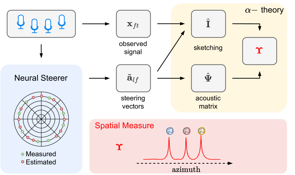
Figure 1: Schematic pipeline of the proposed algorithm.

The SSL problem is inherently non-linear, and many SSL algorithms use deep neural networks (DNNs) to address this challenge by exploiting various audio-spatial features[12, 13, 14, 15]. Convolutional recurrent neural networks have been widely used for capturing SSL features, with recurrent layers benefiting from the time-series nature of audio signals. Attention-based DNNs, such as those in [16, 17], focus on the most relevant features in multichannel data over time. A key challenge is that these data-driven approaches may struggle when applied to data far from the training distribution, particularly in out-of-domain scenarios.

A popular approach for balancing data-driven and fundamental model components is to combine DNN architectures, signal processing, machine learning, or stochastic models [18, 19, 20, 21, 22, 23]. The fusion of stochastic models with signal processing is common due to the stochastic component’s ability to incorporate uncertainty. In [17], a transformer DNN estimates an angle-of-arrival vector following a Gaussian distribution, improving performance over its non-stochastic counterpart. In [23, 24], the signal is modelled as a Gaussian mixture with an inverse Wishart prior on the spatial covariance matrix, improving SSL results by controlling uncertainty in steering vectors (SVs). Alternatively, in [19], the observed mixture signal is modeled as a linear combination of $\alpha$-stable sources, whose SVs enable localization via a spatial measure heatmap. Although its performance was limited when the heatmap was obtained using algebraic SVs, especially with a few microphones, it generally performed well when measured SVs obtained from recorded room impulse responses (RIRs) were used [25]. This raises the need for either a sufficient number of measured SVs or an interpolation technique to spatially upsample limited measurements.

SV interpolation is a traditional topic which includes pure signal processing interpolation, acoustics modeling and array processing. As steering vectors can be extended to head-related transfer functions (HRTFs), RIRs and directivity patterns, several interpolation techniques can be found in related HRTF upsampling [26], sound field reconstruction [27] and array manifolds learning [28]. Recently, physics-informed deep learning (PIDL) approaches that combine the expressiveness of deep learning with guarantees of physical models [27] have shown promising results in the case of scarce measurements.

In this paper, we propose a novel fusion of the Neural Steerer [29], an existing PIDL for steering vector interpolation, with the $\alpha$-stable SSL technique [25]. Our evaluation demonstrates that the proposed method, Sound Localization with Hybrid Alpha-stable Spatial Measure and Neural Steerer (SHAMaNS), outperforms other SSL baselines, particularly in scenarios with few steering vectors measured or high number of sources.

II Background

This section briefly describes the SSL technique based on $\alpha$-stable spatial measure (Section II-A) and the SV interpolation techniques (Section II-B). We work in the short-time Fourier transform (STFT) domain, where a time-frequency (TF) bin is identified by its frequency index $f\in[1,F]$ and time index $t\in[1,T]$ with $F$ and $T$ are the total numbers of frequency bins and time frames, respectively.

II-A $\alpha$-stable Spatial Measure for Sound Source Localization

Following [19, 25], an $M$-channel observed mixture signal $\mathbf{x}_{ft}\in\mathbb{C}^{M}$ is assumed to be a sum of source images propagated from $L$ potential source locations:

$$\mathbf{x}_{ft}=\sum_{l=1}^{L}\mathbf{a}_{lf}s_{lft},$$ (1)

where $\mathbf{a}_{lf}\in\mathbb{C}^{M}$ is the direct-path SV pointing toward $s_{lft}\in\mathbb{C}$ and $l\in[1,L]$ represents one potential source location on a grid (e.g., in the polar or Cartesian coordinate system). Given $\mathbf{x}_{ft}$ and the number of sources of interest $N$, we aim to estimate the locations of $N$ sources ($N<L$).

Each $s_{lft}$ is assumed to follow a complex univariate isotropic $\alpha$-stable distribution [30] with a frequency- and time-invariant scale parameter $\Upsilon_{l}\in\mathbb{R}_{+}$, denoted as $s_{lft}\sim\mathcal{S}_{\alpha}S_{\mathbb{C}}\!\left({\Upsilon_{l}}\right)$. The $N$ active source signals coming from their respective locations can be seen as “outliers” in terms of energy since $\Upsilon_{l^{\prime}}\approx 0$ when $l^{\prime}$ is not a position of an active source. The characteristic exponent $\alpha\in(0,2]$ determines the heaviness of the distribution’s tail: smaller $\alpha$ leads to heavier tails (which allows more outliers), whereas $\alpha=2$ corresponds to the Gaussian distribution. For the non-Gaussian case ($\alpha<2$), it can be shown that $\mathbf{x}_{ft}$ follows a complex isotropic $\alpha$-stable distribution with a unique discrete spatial measure $\bm{\Upsilon}\triangleq[\Upsilon_{1},\dots,\Upsilon_{L}]\in\mathbb{R}_{+}^{L}$ [25].

Due to the absence of an analytic form for the probability density function, we use the time-invariant Lévy exponent $I_{f}(\bm{\theta})\in\mathbb{R}$ given a parameter $\bm{\theta}\in\mathbb{C}^{M}$ to establish a relationship between $\bm{\Upsilon}$, $\mathbf{x}_{ft}$, and $\mathbf{a}_{lf}$ as

$$I_{f}(\bm{\theta})\triangleq-\ln\mathbb{E}[e^{\mathrm{i}\Re(\bm{\theta}^{\mathsf{H}})\mathbf{x}_{ft}}]=\sum_{l=1}^{L}\Upsilon_{l}\left|\bm{\theta}^{\mathsf{H}}{\tilde{\mathbf{a}}}_{lf}\right|^{\alpha},$$ (2)

where $\tilde{\mathbf{a}}_{lf}\triangleq\mathbf{a}_{lf}/\|\mathbf{a}_{lf}\|_{2}^{2}$ is a normalized SV.

Following [25], instead of using a Lévy exponent given a single parameter $\bm{\theta}$ as above, we consider a set of parameters $\bm{\theta}_{lf}\triangleq\tilde{\mathbf{a}}_{lf}$ to provide physical interpretation and use the nonnegative estimator of the Lévy exponent given by

$$\hat{I}_{f}(\tilde{\mathbf{a}}_{lf})=-2\ln\left|\frac{1}{T}\sum_{t=1}^{T}\exp\left(\mathrm{i}\frac{\Re(\tilde{\mathbf{a}}_{lf}^{\mathsf{H}}\mathbf{x}_{ft})}{2^{1/\alpha}}\right)\right|.$$ (3)

By defining $\hat{\mathbf{I}}_{f}\triangleq[\hat{I}_{f}(\tilde{\mathbf{a}}_{1f}),\dots,\hat{I}_{f}(\tilde{\mathbf{a}}_{Lf})]^{\top}\in\mathbb{R}_{+}^{L}$ and $\bm{\Psi}_{f}\triangleq\big{[}\big{|}\tilde{\mathbf{a}}_{lf}^{\mathsf{H}}\tilde{\mathbf{a}}_{l^{\prime}f}\big{|}^{\alpha}\big{]}_{l=1,l^{\prime}=1}^{L,L}\in\mathbb{R}_{+}^{L\times L}$, we have the relation $\hat{\mathbf{I}}_{f}\approx\bm{\Psi}_{f}\bm{\Upsilon}$. Since $\bm{\Upsilon}$ is frequency-independent, we concatenate all $\hat{\mathbf{I}}_{f}$ and $\bm{\Psi}_{f}$ matrices along the frequency axis to form a vector $\hat{\mathbf{I}}\in\mathbb{R}_{+}^{FL}$ and a matrix $\bm{\Psi}\in\mathbb{R}_{+}^{FL\times L}$, respectively, leading to the relation:

$$\hat{\mathbf{I}}\approx\bm{\Psi}\bm{\Upsilon}.$$ (4)

As $\bm{\Psi}$ may still be ill-conditioned making it inversion unstable, we instead minimize the pointwise $\beta$-divergence between the left- and right-hand sides of Eq. (4), while imposing a sparsity penalty constraint on $\bm{\Upsilon}$ [19]. This optimization problem ultimately leads to the following iterative update strategy:

$$\hat{\bm{\Upsilon}}\leftarrow\hat{\bm{\Upsilon}}\odot\frac{\bm{\Psi}^{\top}\left(\left(\bm{\Psi}\hat{\bm{\Upsilon}}\right)^{\beta-2}\odot\hat{\mathbf{I}}\right)}{\bm{\Psi}^{\top}\left(\left(\bm{\Psi}\hat{\bm{\Upsilon}}\right)^{\beta-1}\right)+\lambda},$$ (5)

where $\lambda\in\mathbb{R}_{+}$ is the sparsity penalty coefficient with $a\odot b$ and $\frac{a}{b}$ denote element-wise multiplication and division, respectively.

II-B Steering Vector Interpolation

SVs have been typically used for representing the spatial characteristics of the sound field around an array aperture as function of the probing direction. Given the microphone array geometry and a target location, the algebraic model for the SV is given by

$$\mathbf{a}_{lf}=\exp(2\pi\omega_{f}\mathbf{r}_{l}/cF_{s})/\sqrt{4\pi}\mathbf{r}_{l},$$ (6)

where $\textbf{r}_{l}$ contains the distances between the target location $l$ and the microphone positions in the array, $c$ is the speed of sound, $\omega_{f}$ is the angular frequency in the band $f$, and $F_{s}$ is the sampling frequency.

In real-world environments, frequency-dependent filtering effects, e.g., scattering around the array and pick-up patterns, alter the theoretical shape of the SVs. Although they can be measured accurately, as in [31], measuring them at high spatial resolution may be unfeasible and prohibitive due to the cost and setup complexity. To address this, reliable data-driven interpolation approaches have received significant attention.

For far field applications, it is common to interpolate SVs with respect to location on the sphere centered at the array location. Methods like barycentric interpolation and spherical splines provide a smooth interpolation on the spherical surface (See [26] for a review in case of HRTFs data). Physically motivated methods, such as spherical harmonics (SH) interpolation, are currently the state of the art for such task provided a set of measurements on a predefined grid. The SH expansion of the $m$-th element of SV for the direction of arrival (DOA) $\vartheta_{l}$ is written as

$$a_{lmf}=\sum_{\nu=0}^{\infty}\sum_{\mu=-\nu}^{\nu}c_{\nu\mu,mf}Y_{\nu}^{\mu}(\vartheta_{l}),$$ (7)

where $Y_{\nu}^{\mu}$ is an SH basis of order $\mu$ and degree $\nu$. Given a set of measurements at different $\vartheta_{l}$, the expansion coefficients $c_{\nu\mu,mf}$ are typically estimated by regularized linear regression for each microphone $m$ and frequency band $f$ independently. Unfortunately, these methods lead to poor interpolation when measurements are sparse and randomly distributed [32].

Recent advancement in physics-informed deep learning architectures provides a new solution to increase the spatial resolution of acoustic measurements [33, 27]. Our previous study [29] demonstrated that a coordinate-based neural network, called Neural Steerer (NS), can be used to up-sample steering vectors from a few sparse measurements.

III Proposed Extension

This section introduces the proposed Sound localization with Hybrid Alpha-stable Spatial Measure and Neural Steerer (SHAMaNS).

III-A Mixing Model with Additive Noise

We formulate a new mixing model by introducing an additive noise component $\mathbf{n}_{ft}$ to the model in Eq. (1) as follows:

$$\mathbf{x}_{ft}=\sum_{l=1}^{L}\mathbf{a}_{lf}s_{lft}+\mathbf{n}_{ft},$$ (8)

where $\mathbf{n}_{ft}\sim\mathcal{E}_{\alpha}(\epsilon\mathbb{I}_{M})$ follows a complex isotropic elliptically contoured $\alpha$-stable distribution with $\epsilon\in\mathbb{R}_{+}$ and $\mathbb{I}_{M}\in\mathbb{R}^{M\times M}$ is the identity matrix [22]. The Lévy exponent $I_{f}(\bm{\theta})\in\mathbb{R}$ given $\bm{\theta}\in\mathbb{C}^{M}$ is then expressed as

$$I_{f}(\bm{\theta})=\sum_{l=1}^{L}\Upsilon_{l}\left|\bm{\theta}^{\mathsf{H}}{\tilde{\mathbf{a}}}_{lf}\right|^{\alpha}+C_{\alpha}\left|\bm{\theta}^{\mathsf{H}}\bm{\theta}\right|^{\alpha},$$ (9)

where $C_{\alpha}=(\epsilon/2)^{\alpha/2}$. If we consider a set of $\bm{\theta}_{lf}\triangleq\tilde{\mathbf{a}}_{lf}$ to compute $\bm{\Psi}_{f}$, $\bm{\Upsilon}$, $\mathbf{I}_{f}$ as in Section II-A, we obtain the relation:

$$\mathbf{I}_{f}=\bm{\Psi}_{f}\bm{\Upsilon}+C_{\alpha}\mathbb{1}_{L},$$ (10)

where $\mathbb{1}_{L}$ is an $L$-dimensional vector of ones. Interestingly, deriving the multiplicative update by computing the gradient along $\bm{\Upsilon}$ makes the second term in Eq. $\eqref{eq:new_Levy2}$ vanish and results in the same update formula as in Eq. (5).

This result implies that if $\alpha$ for $\mathbf{x}_{ft}$ is correctly estimated, the noise component is implicitly taken care of and the proposed approach can extract only the desired signals. From this viewpoint, we claim that a correct estimation of $\alpha$, rather than a cherry-picking approach [25, 19], is essential for the algorithm to work correctly. Note that the spatial measure of $\mathbf{n}_{ft}$ is not unique in the Gaussian case so estimating the spatial measure from $\mathbf{x}_{ft}$ is theoretically incorrect in this case [30].

III-B Observation Normalization for Increasing Robustness

We propose to normalize $\mathbf{x}_{ft}$ for computing Eq. (10). $\alpha$-stable realizations for $\alpha<2$ would have outliers that benefit SSL, but a sound source with low energy may not be correctly identified, leading to poor SSL results in practice. According to the covariation formula [30, p. 87], the spatial measure remains computationally unchanged up to a scale parameter independent of the direction. We consequently choose to use $\tilde{\mathbf{x}}_{ft}\triangleq\mathbf{x}_{ft}/\|\mathbf{x}_{ft}\|_{p}^{p}$, where $p<\alpha$ since the norm can be theoretically infinite for $p\geq\alpha$.

III-C Fusion with Neural Steerer

Ideally, we can interchangeably use algebraic SVs or measured SVs as $\bm{\theta}_{lf}$ to compute $\hat{\mathbf{I}}$ and $\bm{\Psi}$. However, algebraic SVs significantly differ from SVs measured in the real world, resulting in poor SSL performance in practice. Since measuring SVs is costly, this paper proposes to generate a large set of SVs from a small set of measured SVs. To this end, we modify the Neural Steerer (NS) model [29]. Instead of learning the mapping from a DOA to its steering vector filter, we use a coordinate-based neural network to estimate the SH expansion coefficients $c_{\nu\mu,mf}$ for a given microphone index, DOA Cartesian coordinate and frequency band. The expressiveness of the deep learning helps to resolve the higher SH coefficients. The extensive study of the influence of different interpolation methods on SSL performances is out of the scope of this work.

We assume that we have $\mathbf{a}_{lf}^{\text{NS}}\approx\mathbf{a}_{lf}^{\text{true}}+\mathbf{e}_{f}$ where $\mathbf{a}_{lf}^{\text{NS}},\mathbf{a}_{lf}^{\text{true}},\mathbf{e}_{f}$ denote the NS-reconstructed SV, the true SV, and the error, respectively. As is common for interpolation methods of acoustic measurements, reconstruction error increases with the frequencies [27]. Consequently, error appears impulsive at certain frequencies and directions, thus, we can assume that it is incorporated into the noise component $\mathbf{n}_{ft}$.

IV Evaluation

This section presents the SSL performance of SHAMaNS in comparison to two widely-used wideband SSL methods: MUSIC [7] and SRP-PHAT [8]. Each method may use the measured oracle SVs (“Ref.”), the corresponding algebraic SVs (“Alg.”), or the interpolated SVs generated by NS. The SSL performances were evaluated in terms of the angular error $d(\vartheta,\hat{\vartheta})$ on the unit circle and the accuracy for $d(\vartheta,\hat{\vartheta})<15^{\circ}$.

IV-A Settings

We used the SVs measured using head-worn smartglasses, featuring four microphones on the frame and binaural in-ear microphones ($M=6$), from the SPeech Enhancement for Augmented Reality (SPEAR) challenge dataset [34]. From these $1020$ anechoic SVs measured using a dummy head, we randomly sampled $N_{\text{SV}}=[8,16,32,64,128]$ measurements on the entire sphere to fit an NS model (“NS-$N_{\text{SV}}$”).

We generated 30 different acoustic scenes for each investigation below by varying the number of sources $N$, the signal-to-noise ratio (SNR) for additive white Gaussian noise, and reverberation time (RT60). For each acoustic scene, we generated RIRs and convolved them with speech utterances from the VCTK corpus (ver. 0.92) [35]. To obtain directional responses, each RIR was spatially convolved with the corresponding SV which is interpolated using SH interpolation from the oracle measured SVs. The microphone array was placed randomly in a shoebox room with a size of $6\times 4\times 3$ $\mathrm{m}$. The potential source locations were $6$ degrees apart ($L=60$) on the azimuthal plane (elevation $=0$) at a distance of $1.7$ $\mathrm{m}$ from the array. The sources were then randomly placed at least $12$ degrees apart.

All data were sampled at $F_{s}=48$ kHz. The STFT frame size was 768 samples with 50% overlap between frames and computed with a Hann window. Otherwise specified, only positive frequencies up to 8 kHz were considered.

For SHAMaNS, we estimated $\alpha$ from the mixture as in [36], fixed $p=1$, and then optimized the parameters using Eq. (5) with $\beta=1$ and $\lambda=10^{-3}$ for 500 iterations. The estimated spatial measure was initialized as $\hat{\bm{\Upsilon}}\leftarrow\mathbf{1}_{L}$. For MUSIC, we used either the only largest eigenvector (“MUSIC-1”) or the first four largest eigenvectors (“MUSIC-4”) to define the signal subspace. In the case of $N>1$, the Hungarian algorithm was used to find the best-estimated source permutation.

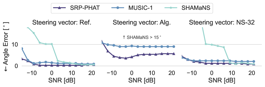
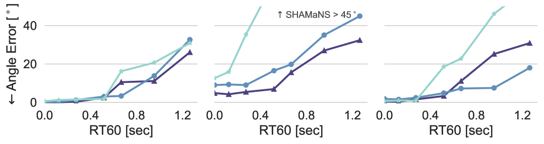
Figure 2: Average angular errors for the different SNRs (top) and RT60s (bottom) using the different localization methods and steering vector models.

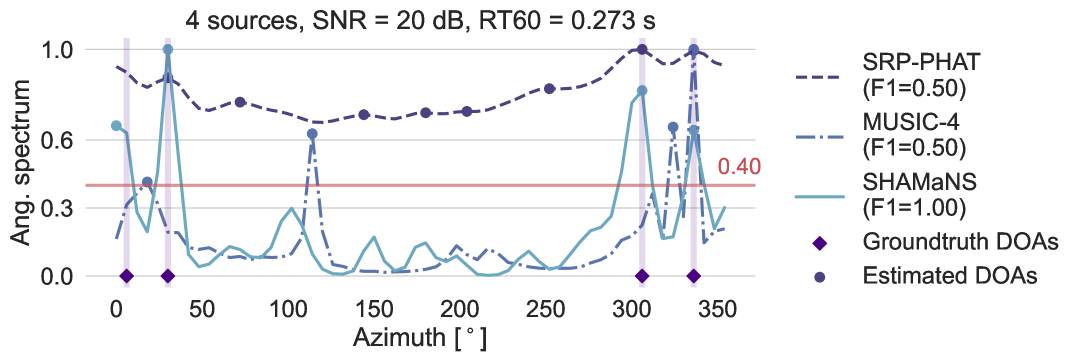
Figure 3: SSL cost function (angular spectrum) for different localization methods. Horizontal lines represent the threshold for peak-picking methods.

IV-B Results

Fig. 2 reports the average angular error against different noise and reverberation levels in a single sound source case ($N=1$) with 30 random simulations for each value of SNR and RT60. SHAMaNS was shown to have comparable performances for positive SNR and moderate reverberation when measured or interpolated SVs were used, leading to an average error of $0.98^{\circ}\pm 2.45^{\circ}$ for SHAMaNS, $1.07^{\circ}\pm 2.31^{\circ}$ for MUSIC-1, and $0.38^{\circ}\pm 1.47^{\circ}$ for SRP-PHAT. The performances of all methods dropped when the algebraic SVs were used, where SRP-PHAT outperformed with an average error of $5.48^{\circ}\pm 7.50^{\circ}$.

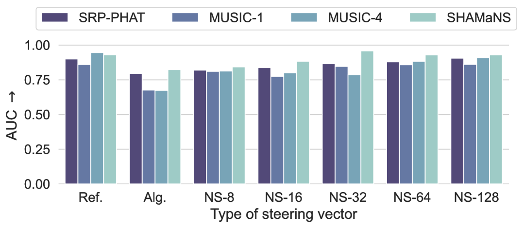
Figure 4: Area under the ROC curve for the number of source classifications using different thresholds of the angular spectrum. Comparison is for different localization methods using different steering vector models.

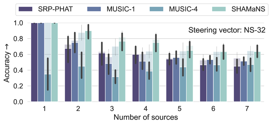
Figure 5: Accuracy (success for angular error less than 15 degrees) for different localization methods and steering vector models. RT60=0.123 ms, SNR = 20 dB. Performances with SV = Ref. are reported in the background in transparency.

Next, we investigated the impact of the SV interpolation quality on the SSL performance when the number of sources $N$ is unknown. This task was achieved by thresholding the normalized SSL method’s cost function for the candidate DOAs (shown in Fig 3) and counting the highest peaks. By considering it as a classification task, we then computed the area under the curve (AUC) using different value thresholds to perform the classification. The performance metrics were computed setting $N=3$, SNR $=20$ dB and RT60 $=0.273$ ms. The results in Fig. 4 show that SHAMaNS and MUSIC-4 outperformed the other baselines. As expected, using interpolation methods that used more observations improves the performance. The oracle SSL performance could be obtained with only 10% of the initial measurements and a reasonable performance with only 32 random measurements.

Finally, we studied the accuracy of locating $N$ sound sources as a function of their numbers. The results in Fig. 5 show that most of the methods could estimate source location when $N<5$ with accuracy above 55% when either oracle or sufficiently well-interpolated SVs (NS-32). Performances dropped for higher values of $N$, while SHAMaNS outperformed the baseline methods for locating from 2 to 6 concurrent sources, which happened in most practical use cases.

V Conclusion & Future Work

This study introduced a novel approach that combines NeuralSteerer, a deep neural network-based physics-informed steering vector model, with a theoretically grounded source localization technique derived from $\alpha$-stable theory. We provide a theoretical justification for this hybrid fusion by incorporating the error model of NeuralSteerer into the additive impulsive noise framework of the $\alpha$-stable model. Our results demonstrate that the proposed method achieves superior performance for localizing multiple sound sources, even when only a limited number of measured steering vectors are available. Future work will study the interaction between different interpolation and localization methods.

References

- [1] R. M. Corey, “Microphone array processing for augmented listening,” Ph.D. dissertation, University of Illinois at Urbana-Champaign, 2019.
- [2] R. Gupta, J. He, R. Ranjan, W.-S. Gan, F. Klein, C. Schneiderwind, A. Neidhardt, K. Brandenburg, and V. Välimäki, “Augmented/mixed reality audio for hearables: Sensing, control, and rendering,” IEEE Signal Process. Mag., vol. 39, no. 3, pp. 63–89, 2022.
- [3] R. Jalayer, M. Jalayer, A. Mor, C. Orsenigo, and C. Vercellis, “ConvLSTM-based sound source localization in a manufacturing workplace,” Comput. Ind. Eng., vol. 192, p. 110213, 2024.
- [4] J. Wang, Y. He, D. Su, K. Itoyama, K. Nakadai, J. Wu, S. Huang, Y. Li, and H. Kong, “SLAM-based joint calibration of multiple asynchronous microphone arrays and sound source localization,” IEEE Trans. Robot., vol. 40, pp. 4024–4044, 2024.
- [5] A. Madan and L. Li, “Acoustic simultaneous localization and mapping for autonomous driving,” in Proc. IEEE ICCSI, 2024, pp. 1–6.
- [6] I. Marques, J. Sousa, B. Sá, D. Costa, P. Sousa, S. Pereira, A. Santos, C. Lima, N. Hammerschmidt, S. Pinto, and T. Gomes, “Microphone array for speaker localization and identification in shared autonomous vehicles,” Electronics, vol. 11, no. 5, p. 766, 2022.
- [7] R. Schmidt, “Multiple emitter location and signal parameter estimation,” vol. 34, no. 3, pp. 276–280, 1986.
- [8] J. H. DiBiase, H. F. Silverman, and M. S. Brandstein, “Robust localization in reverberant rooms,” in Microphone Arrays: Signal Processing Techniques and Applications, M. Brandstein and D. Ward, Eds. Springer, 2001, pp. 157–180.
- [9] D. Salvati, C. Drioli, and G. L. Foresti, “Incoherent frequency fusion for broadband steered response power algorithms in noisy environments,” IEEE Signal Process. Lett., vol. 21, no. 5, pp. 581–585, 2014.
- [10] K. Nakamura, K. Nakadai, F. Asano, Y. Hasegawa, and H. Tsujino, “Intelligent sound source localization for dynamic environments,” in Proc. IEEE/RSJ IROS, 2009, pp. 664–669.
- [11] M. Cobos, A. Marti, and J. J. Lopez, “A modified SRP-PHAT functional for robust real-time sound source localization with scalable spatial sampling,” IEEE Signal Process. Lett., vol. 18, no. 1, pp. 71–74, 2010.
- [12] S. Adavanne, A. Politis, and T. Virtanen, “Differentiable tracking-based training of deep learning sound source localizers,” in Proc. IEEE WASPAA, 2021, pp. 211–215.
- [13] D. Rho, S. Lee, J. Park, T. Kim, J. Chang, and J. Ko, “A combination of various neural networks for sound event localization and detection,” DCASE Challenge, Tech. Rep., 2021.
- [14] B. Yang, H. Liu, and X. Li, “Learning deep direct-path relative transfer function for binaural sound source localization,” IEEE/ACM Trans. Audio, Speech, Language Process., vol. 29, pp. 3491–3503, 2021.
- [15] A. S. Subramanian, C. Weng, S. Watanabe, M. Yu, Y. Xu, S.-X. Zhang, and D. Yu, “Directional ASR: A new paradigm for E2E multi-speaker speech recognition with source localization,” in Proc. IEEE ICASSP, 2021, pp. 8433–8437.
- [16] Y. Cao, T. Iqbal, Q. Kong, F. An, W. Wang, and M. D. Plumbley, “An improved event-independent network for polyphonic sound event localization and detection,” in Proc. IEEE ICASSP, 2021, pp. 885–889.
- [17] C. Schymura, B. Bönninghoff, T. Ochiai, M. Delcroix, K. Kinoshita, T. Nakatani, S. Araki, and D. Kolossa, “PILOT: Introducing transformers for probabilistic sound event localization,” in Proc. INTERSPEECH, 2021, pp. 2117–2121.
- [18] V. Letzelter, M. Fontaine, M. Chen, P. Pérez, S. Essid, and G. Richard, “Resilient multiple choice learning: A learned scoring scheme with application to audio scene analysis,” in Proc. NeurIPS, vol. 36, 2023, pp. 6001–6013.
- [19] M. Fontaine, C. Vanwynsberghe, A. Liutkus, and R. Badeau, “Sketching for nearfield acoustic imaging of heavy-tailed sources,” in Proc. Int. Conf. Latent Variable Anal. Signal Separation, 2017, pp. 80–88.
- [20] J. Azcarreta, N. Ito, S. Araki, and T. Nakatani, “Permutation-free CGMM: Complex gaussian mixture model with inverse wishart mixture model based spatial prior for permutation-free source separation and source counting,” in Proc. IEEE ICASSP, 2018, pp. 51–55.
- [21] N. Q. Duong, E. Vincent, and R. Gribonval, “Spatial location priors for gaussian model based reverberant audio source separation,” EURASIP J. Adv. Signal Process., vol. 2013, p. 149, 2013.
- [22] M. Fontaine, D. Di Carlo, K. Sekiguchi, A. A. Nugraha, Y. Bando, and K. Yoshii, “Elliptically contoured alpha-stable representation for MUSIC-based sound source localization,” in Proc. EUSIPCO, 2022, pp. 26–30.
- [23] Y. Sumura, D. Di Carlo, A. A. Nugraha, Y. Bando, and K. Yoshii, “Joint audio source localization and separation with distributed microphone arrays based on spatially-regularized multichannel NMF,” in Proc. IWAENC, 2024, pp. 145–149.
- [24] F. Asano, H. Asoh, and K. Nakadai, “Sound source localization using joint bayesian estimation with a hierarchical noise model,” IEEE Audio, Speech, Language Process., vol. 21, no. 9, pp. 1953–1965, 2013.
- [25] M. Fontaine, C. Vanwynsberghe, A. Liutkus, and R. Badeau, “Scalable source localization with multichannel -stable distributions,” in Proc. EUSIPCO, 2017, pp. 11–15.
- [26] V. Bruschi, L. Grossi, N. A. Dourou, A. Quattrini, A. Vancheri, T. Leidi, and S. Cecchi, “A review on head-related transfer function generation for spatial audio,” Applied Sciences, vol. 14, no. 23, p. 11242, 2024.
- [27] S. Koyama, J. G. Ribeiro, T. Nakamura, N. Ueno, and M. Pezzoli, “Physics-informed machine learning for sound field estimation: Fundamentals, state of the art, and challenges,” IEEE Signal Process. Mag., vol. 41, no. 6, pp. 60–71, 2025.
- [28] A. Manikas, Differential geometry in array processing. Imperial College Press, 2004.
- [29] D. Di Carlo, A. A. Nugraha, M. Fontaine, Y. Bando, and K. Yoshii, “Neural steerer: Novel steering vector synthesis with a causal neural field over frequency and direction,” in Proc. IEEE ICASSPW, 2024, pp. 740–744.
- [30] G. Samorodnitsky and M. S. Taqqu, Stable Non-Gaussian Random Processes: Stochastic Models with Infinite Variance. Chapman and Hall/CRC, 1994.
- [31] J. Donley, V. Tourbabin, J.-S. Lee, M. Broyles, H. Jiang, J. Shen, M. Pantic, V. K. Ithapu, and R. Mehra, “EasyCom: An augmented reality dataset to support algorithms for easy communication in noisy environments,” arXiv e-print, pp. 1–9, 2021, arXiv:2107.04174v2.
- [32] D. Bau, J. M. Arend, and C. Pörschmann, “Estimation of the optimal spherical harmonics order for the interpolation of head-related transfer functions sampled on sparse irregular grids,” Frontiers in Signal Processing, vol. 2, p. 884541, 2022.
- [33] X. Chen, F. Ma, A. Bastine, P. Samarasinghe, and H. Sun, “Sound field estimation around a rigid sphere with physics-informed neural network,” in Proc. APSIPA ASC, 2023, pp. 1984–1989.
- [34] P. Guiraud, S. Hafezi, P. A. Naylor, A. H. Moore, J. Donley, V. Tourbabin, and T. Lunner, “An introduction to the speech enhancement for augmented reality (SPEAR) challenge,” in Proc. IWAENC, 2022, pp. 1–5.
- [35] J. Yamagishi, C. Veaux, and K. MacDonald, “CSTR VCTK corpus: English multi-speaker corpus for CSTR voice cloning toolkit,” 2019.
- [36] M. Fontaine, K. Sekiguchi, A. A. Nugraha, Y. Bando, and K. Yoshii, “Alpha-stable autoregressive fast multichannel nonnegative matrix factorization for joint speech enhancement and dereverberation.” in Proc. INTERSPEECH, 2021, pp. 661–665.