Relativistic corrections to exclusive photoproduction of Quarkonia near-threshold

Abstract

Non-relativistic QCD (NRQCD) is used to calculate the relativistic correction to the amplitude for exclusive photoproduction of vector Quarkonia in the near-threshold region within the generalized parton distribution (GPD) framework. The relativistic corrections are found to be large for $J/\psi$. Cross-sections for both $J/\psi$ and $\Upsilon$ are calculated with the former being compared to the data. We also demonstrate the presence of endpoint divergences for the relativistic correction away from the near-threshold regime.

1 Introduction

An important goal of quantum chromodynamics (QCD) is to explain the properties of nucleons in terms of the underlying partons. One step in this direction is elucidating the spatial distribution of the partons in a nucleon encoded in non-perturbative quantities called generalized parton distributions (GPDs) Muller:1994ses ; Radyushkin:1997ki ; Ji:1996ek . These GPDs can be accessed in exclusive reactions like deeply virtual Compton scattering and deeply virtual meson production. With the already running experiments at Thomas Jefferson Laboratory (JLab) Adderley:2024czm and the upcoming Electron-Ion Collider (EIC) AbdulKhalek:2021gbh , significant progress will be made in precision measurement of these quantities. Thus higher order and higher power calculations are warranted on the theoretical side. In the present work, we take a first step towards a full analysis of power corrections by determining a unique subset of such corrections for processes with a heavy quarkonia.

Exclusive production of a vector meson has been studied in different kinematical limits using various methods. Within the perturbative QCD (pQCD) framework, calculations have been performed for the high energy and/or small-$x$ limit in the leading logarithmic approximation within the color dipole Nikolaev:1990ja ; Mueller:1993rr and $k_{T}$-factorization approaches Ryskin:1992ui ; Brodsky:1994kf ; Kuraev:1998ht ; Ivanov:1999pb ; Ivanov:2002ef . For heavy vector mesons (HVM), exclusive electroproduction and photoproduction have also been studied at next-to-leading order (NLO) Ivanov:2004vd ; Chen:2019uit ; Flett:2021ghh based on the collinear factorization method Collins:1996fb when $W^{2}\gg M_{V}^{2},-t$. Here $W$ is the invariant mass of the photon-proton system, $M_{V}$ is the mass of the HVM, and $t$ is the invariant momentum transfer squared. For HVM production in the near-threshold limit, we also implicitly assume the hierarchy $M_{V}\gg M_{N}$, where $M_{N}$ is the nucleon mass. The other kinematic region is the near-threshold region, characterized by $W^{2}\sim M_{V}^{2}\gg-t$. In both of these limits the amplitude has been shown to factor into gluon GPDs for both electroproduction Boussarie:2020vmu and photoproduction Guo:2021ibg ; Sun:2021pyw ; Guo:2023pqw at leading power (LP). Moreover in Boussarie:2020vmu ; Guo:2021ibg it has been shown that the amplitude in the threshold limit is directly related to gluon gravitational form factors (GFFs).

In this paper we study the relativistic correction to photoproduction of vector Quarkonia near-threshold following the strategy of Guo:2023pqw , where the nonperturbative dynamics of the proton is encoded in the moments of GPD. Similar relativistic corrections have been studied before, but for electroproduction in the high-energy/small-$x$ limit Hoodbhoy:1996zg , which we will not study here. As we will show, relativistic corrections are large in the near-threshold limit for photoproduction and thus need to be taken into account to explain data from the GlueX collaboration GlueX:2019mkq ; GlueX:2023pev in the low $W$ region.

The rest of the paper is organized as follows. In Sec. 2 we discuss the collinear factorization and Non-relativistic QCD framework and use it to calculate the relativistic correction to the amplitude. In Sec. 3 we show the cross-section for both $J/\psi$ and $\Upsilon$, where we compare the former with experimental results. Finally in Sec. 4 we provide a summary and outlook for future work.

2 Amplitude for $\gamma(q)+N(p)\rightarrow V(P_{V})+N(p^{\prime})$

Exclusive photoproduction of quarkonium is mediated via two-parton exchange and, unlike deep inelastic scattering, the incoming nucleon does not break apart but instead recoils with a different momentum. The production of the $Q\bar{Q}$ pair and its subsequent recombination into an HVM state can be calculated in the nonrelativistic QCD (NRQCD) framework Caswell:1985ui ; Bodwin:1994jh ; Braaten:1993rw ; Fleming:1997fq ; Luke:1999kz ; Brambilla:1999xf ; Bodwin:2007ga ; Copeland:2023wbu which is an expansion in $\alpha_{s}$ and $v$, the relative velocity of the quark-antiquark pair. Projecting the $Q\bar{Q}$ pair onto the HVM gives the NRQCD long distance matrix elements (LDMEs). At leading order in the $v$ expansion there is only one LDME which is related to the HVM wavefunction at the origin. Thus using NRQCD and the collinear expansion, the amplitude for this process can be expressed in a factored form consisting of a short-distance hard matching coefficient, the LDME, and the gluon GPD which parametrizes the dynamics of gluons in the recoiling proton at the nonperturbative scale.

2.1 Kinematics

For the purpose of this calculation, we define the lightcone coordinates in terms of the collinear vector $n^{\mu}=(1,0,0,1)$ and the anticollinear vector $\bar{n}^{\mu}=(1,0,0,-1)$. The calculation is most conveniently done in the Ji frame, where the mean of the large lightcone momentum component of the incoming and outgoing proton is taken along $n^{\mu}$. In the near-threshold limit, the momentum decomposition for the incoming nucleon $p$, the photon $q$, the outgoing nucleon $p^{\prime}$ and the HVM $P_{V}$ in terms of the light-cone basis vectors is:

$$p^{\mu}=(1+\xi)P^{-}\frac{n^{\mu}}{2}+(1-\xi)\frac{M_{N}^{2}-\frac{t}{4}}{P^{-}}\frac{\bar{n}^{\mu}}{2}-\frac{\Delta^{\mu}_{\perp}}{2}\,,$$

$$q^{\mu}=-\frac{2\xi P^{-}}{M^{2}_{V}}\Big{[}(1-\xi^{2})\frac{t}{4}+\xi^{2}M_{N}^{2}\Big{]}\frac{n^{\mu}}{2}+\frac{M^{2}_{V}}{2\xi P^{-}}\Big{[}1+4\xi^{2}\frac{M_{N}^{2}-\frac{t}{4}}{M^{2}_{V}}\Big{]}\frac{\bar{n}^{\mu}}{2}+\frac{\Delta^{\mu}_{\perp}}{2}\,,$$

$$p^{\prime\mu}=(1-\xi)P^{-}\frac{n^{\mu}}{2}+(1+\xi)\frac{M_{N}^{2}-\frac{t}{4}}{P^{-}}\frac{\bar{n}^{\mu}}{2}+\frac{\Delta^{\mu}_{\perp}}{2}\,,$$

$$P_{V}^{\mu}=\frac{2\xi P^{-}}{M^{2}_{V}}\Big{[}M^{2}_{V}-(1-\xi^{2})\frac{t}{4}-\xi^{2}M_{N}^{2}\Big{]}\frac{n^{\mu}}{2}+\frac{M^{2}_{V}}{2\xi P^{-}}\frac{\bar{n}^{\mu}}{2}-\frac{\Delta^{\mu}_{\perp}}{2}\,,$$ (1)

where $p^{2}=p^{\prime\,2}=M_{N}^{2}$, $q^{2}=0$, and $P_{V}^{2}=M_{V}^{2}$. We take the independent kinematic variables to be $P^{-}$, $\xi$ and $t$. Here $P^{-}=\bar{n}\cdot(p^{\prime}+p)/2$, is the average of the largest momentum components of the incoming and outgoing nucleons, $t=(p^{\prime}-p)^{2}$ is the square of the momentum transfer, and $\xi=-\frac{\bar{n}\cdot(p^{\prime}-p)}{\bar{n}\cdot(p^{\prime}+p)}$, the skewness parameter, parametrizes the change in the collinear momentum of the nucleon. Note that the magnitude of the perpendicular component is constrained to be $\vec{\Delta}_{\perp}^{2}=(1-\xi^{2})t+4\xi^{2}M_{N}^{2}$. To obtain the decomposition in Eq. (2.1) we have taken $-t,M_{N}^{2}\ll M_{V}^{2}$ and only retained terms up to $O\left(M_{N}^{2}/M^{2}_{V}\right)$ and $O\left(t/M^{2}_{V}\right)$. To this order, the invariant mass $W^{2}\equiv(q+p)^{2}=M_{V}^{2}(1+\xi)/(2\xi)+M_{N}^{2}(1+2\xi)-t(1+\xi)/2$.

The threshold region can be defined by the limit where $1-\xi\sim M_{N}/M_{V}\sim t/M_{V}^{2}\ll 1$. In this region Guo:2021ibg , $\xi\to 1$, $W^{2}\simeq(M_{V}+M_{N})^{2}$ and $-t\sim O(M_{N}M_{V})$, where this last scaling relation can be seen most easily from the kinematics bounds $-t_{-}<-t<-t_{+}$ where

$$-t_{\pm}= \frac{(W^{2}+M_{N}^{2})(W^{2}-M_{V}^{2}+M_{N}^{2})}{2W^{2}}$$ (2)

$$\pm\frac{(W^{2}-M_{N}^{2})\sqrt{(W^{2}-(M_{V}+M_{N})^{2})(W^{2}-(M_{V}-M_{N})^{2})}}{2W^{2}}-2M_{N}^{2}\,.$$

(These bounds are Lorentz invariant but are derived most easily in the center-of-mass frame.) This has implications for $J/\psi$ since kinematic corrections (dependence of the hard matching coefficient on $t$) and subleading GPD corrections, which go as $-t/W^{2}\sim O(M_{N}/M_{V})$, are the same order as the relativistic corrections $v^{2}$. For the present work we do not consider these power correction and so terms which are proportional to $t$ and $M_{N}^{2}$ in Eq.(2.1) are neglected in the calculation of the hard matching coefficient.

2.2 Projection onto Nonperturbative Matrix Elements

At lowest order in $\alpha_{s}$, the on-shell heavy quark-antiquark pair is produced via two gluon exchange in the partonic processes, which correspond to $\gamma(q)+g(p_{1})\rightarrow g(p_{2})+Q(p_{3})+\bar{Q}(p_{4})$ in the DGLAP region ($|x|>|\xi|$) or $\gamma(q)+g(p_{1})+g(-p_{2})\rightarrow Q(p_{3})+\bar{Q}(p_{4})$ in the ERBL region ($|x|<|\xi|$). The matrix element which extracts gluons from the proton is given by the gluon GPD correlator $F^{g}(x,\xi,t)$, defined by

$$F^{g}(x,\xi,t)=\frac{1}{(P^{-})^{2}}\int\frac{d\lambda}{2\pi}e^{i\lambda x}\,\bar{n}_{\mu}\bar{n}_{\nu}\left\langle p^{\prime}\left|G^{\mu\sigma}_{a}\left(-\frac{\lambda\bar{n}}{2}\right)W\Bigl{[}-\frac{\lambda\bar{n}}{2},\frac{\lambda\bar{n}}{2}\Bigr{]}G^{\nu}_{a\sigma}\left(\frac{\lambda\bar{n}}{2}\right)\right|p\right\rangle,$$ (3)

where $W[b,a]=P\exp(ig\int_{a}^{b}ds\cdot A)$ denotes a straight Wilson line from $a$ to $b$. To probe this GPD operator it suffices to take the two gluons to have momenta

$$p_{1}^{\mu}=(x+\xi)P^{-}\frac{n^{\mu}}{2},\qquad p_{2}^{\mu}=(x-\xi)P^{-}\frac{n^{\mu}}{2}\,.$$ (4)

In the GPD factorization theorem the momentum fraction $x$ will appear in both the hard matching coefficient and the GPDs, and is integrated over. The momenta of the heavy quark-antiquark pair can be expressed in terms of the total momentum $P_{V}$ and the relative momentum of the pair $k\sim m_{Q}v$, with $m_{Q}$ the heavy quark mass:

$$p_{3}=\frac{1}{2}P_{V}+k$$

$$p_{4}=\frac{1}{2}P_{V}-k.$$ (5)

There are six Feynman diagrams contributing to the amplitude as shown in Fig.1.

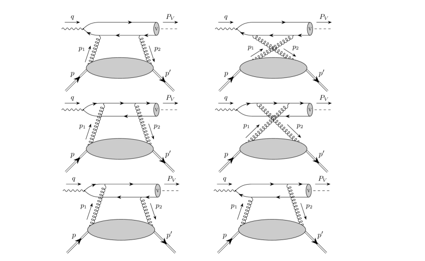
Figure 1: Feynman diagrams required for the calculation of the cross section both at leading power and with relativistic corrections.

The amplitude can in general be written as

$$\mathcal{M} =\bar{u}(p_{3})\mathcal{A}^{(\alpha\beta)}v(p_{4})\varepsilon_{\alpha}(p_{1})\varepsilon^{*}_{\beta}(p_{2})$$

$$=\text{Tr}\left[\mathcal{A}^{(\alpha\beta)}v(p_{4})\bar{u}(p_{3})\right]\varepsilon_{\alpha}(p_{1})\varepsilon^{*}_{\beta}(p_{2})$$

$$\equiv\mathcal{M}^{(\alpha\beta)}\varepsilon_{\alpha}(p_{1})\varepsilon^{*}_{\beta}(p_{2})\,,$$ (6)

where $\mathcal{A}$ is a matrix that acts on spinors with both Dirac and color indices and $\varepsilon_{\alpha}(p_{1}),\varepsilon^{*}_{\beta}(p_{2})$ are the polarization vectors for the incoming and outgoing gluon respectively. For later convenience we have indicated the Lorentz indices contracting with the gluon polarization vectors in parentheses. By replacing $v(p_{4})\bar{u}(p_{3})$ with projection operators one can project the $Q\bar{Q}$ state onto a particular spin and color configuration. For the spin triplet, color singlet configuration the projection operator is

$$\Pi^{Q\bar{Q}}_{3}(p_{4},p_{3})=\frac{1}{\sqrt{2}M_{V}(M_{V}+2m_{Q})}(\not{p}_{4}-m_{Q})\not{\varepsilon}^{*}_{V}(\not{P}_{V}+M_{V})(\not{p}_{3}+m_{Q})\otimes\left(\frac{1}{\sqrt{N_{c}}}\bf{1}\right),$$ (7)

where $N_{c}=3$, $\varepsilon^{*}_{V}$ is the quarkonium spin polarization vector satisfying $\varepsilon^{*}_{V}\cdot\varepsilon_{V}=-1$ and $P_{V}\cdot\varepsilon_{V}=0$, and $\bf{1}$ in the last factor is the unit color matrix. We also express $M_{V}$ in terms of the the heavy quarkmass $m_{Q}$ via the relation $M_{V}^{2}=4(m_{Q}^{2}-k^{2})$. Using the projection operator the matrix element takes the form

$$\mathcal{M}^{(\alpha\beta)}[Q\bar{Q}(S=1)]= \text{Tr}\left[\mathcal{A}^{(\alpha\beta)}\Pi^{Q\bar{Q}}_{3}\right]=\mathcal{M}^{(\alpha\beta)}_{\mu\nu}\varepsilon_{\gamma}^{\mu}\varepsilon_{V}^{*\nu}$$

$$= \left(\mathcal{M}^{(0)(\alpha\beta)}_{\mu\nu}+\mathcal{M}^{(1)(\alpha\beta\rho)}_{\mu\nu}k_{\rho}+\mathcal{M}^{(2)(\alpha\beta)}_{\mu\nu\rho\sigma}k^{\rho}k^{\sigma}+\dots\right)\varepsilon_{\gamma}^{\mu}\varepsilon_{V}^{*\nu}$$ (8)

where in the second line the amputated amplitude $\mathcal{M}^{(\alpha\beta)}_{\mu\nu}$ has been expanded in powers of $k$. The amplitude for the spin-triplet quarkonium state $V$ at leading order in $v$ is

$$\mathcal{M}^{(\alpha\beta)}[V]=\left(\frac{\langle\mathcal{O}_{1}(^{3}S_{1})\rangle_{V}}{N_{c}M_{V}}\right)^{1/2}\mathcal{M}^{(0)(\alpha\beta)}_{\mu\nu}\varepsilon_{\gamma}^{\mu}\varepsilon_{S}^{*\nu}\,,$$ (9)

where $\langle\mathcal{O}_{1}(^{3}S_{1})\rangle_{V}\equiv\langle V|\chi^{\dagger}\boldsymbol{\sigma}\psi\cdot\chi^{\dagger}\boldsymbol{\sigma}\psi|V\rangle$ is the nonrelativistic LDME for the color singlet, spin triplet operator. Matching the amplitude onto the gluon GPD correlator $F^{g}(x,\xi,t)$ is achieved by the replacement

$$\epsilon_{a}^{\alpha}(p_{1})\epsilon_{b}^{*\beta}(p_{2})\rightarrow\frac{\delta_{ab}}{(N_{c}^{2}-1)}\frac{g^{\alpha\beta}_{\perp}}{2(d-2)}\frac{F^{g}(x,\xi,t)}{(x-\xi+i\epsilon)(x+\xi-i\epsilon)}\,,$$ (10)

where $a,b$ are color indices in the adjoint representation, $g^{\alpha\beta}_{\perp}\equiv g^{\alpha\beta}-\frac{1}{2}n^{\alpha}\bar{n}^{\beta}-\frac{1}{2}\bar{n}^{\alpha}n^{\beta}$ and the factor of $d-2$ in the denominator is to average over the transverse gluon polarizations in $d$-dimensions.

2.3 Relativistic Correction and Gravitational Form Factors

Before we discuss the relativistic corrections it is instructive to review the leading power calculations. There are six diagrams which contribute to the amplitude at leading order in $\alpha_{s}$. Using the projections discussed in Sec.2.2, the amplitude can be readily evaluated

$$\mathcal{M}^{(0)}[V]=\frac{8\sqrt{2}\pi g_{e}e_{Q}\alpha_{s}}{3}\left(\frac{\langle\mathcal{O}_{1}(^{3}S_{1})\rangle_{V}}{M_{V}}\right)^{1/2}\left(\varepsilon_{\gamma}^{\perp}\cdot\varepsilon_{V}^{*\perp}\right)\int_{-1}^{1}dx\,C^{(0)}(x,\xi)F^{g}(x,\xi,t)$$ (11)

where the hard matching coefficient is

$$C^{(0)}(x,\xi)=-\frac{1}{2m_{Q}}\frac{1}{(x-\xi+i\epsilon)(x+\xi-i\epsilon)}.$$ (12)

This reproduces the LO amplitude in Guo:2021ibg with the identification of the NRQCD matrix element with the wavefunction at the origin $\langle\mathcal{O}_{1}(^{3}S_{1})\rangle_{V}=2N_{c}|\psi(0)|^{2}$ and $M_{V}=2m_{Q}$ at leading power in the vacuum saturation approximation. Parametrizing the gluon GPD correlator in terms of a nucleon spinor $U(p)$ we can write

$$F_{g}(x,\xi,t)=\frac{1}{P^{-}}\left[H_{g}(x,\xi,t)\bar{U}(p^{\prime})\frac{\not{\bar{n}}}{2}U(p)+E_{g}(x,\xi,t)\bar{U}(p^{\prime})\frac{i\sigma^{\mu\nu}(p^{\prime}-p)_{\nu}}{2M_{N}}U(p)\frac{\bar{n}_{\mu}}{2}\right],$$ (13)

where $H_{g}$ and $E_{g}$ are (scalar) GPDs.

Since in the near-threshold limit $\xi\sim 1$ one can expand the hard matching coefficient about $|x|\ll|\xi|$, and express the convolution in terms of even moments of the GPD

$$\mathcal{M}^{(0)}[V]=\frac{4\sqrt{2}\pi g_{e}e_{Q}\alpha_{s}}{3m_{Q}}\left(\frac{\langle\mathcal{O}_{1}(^{3}S_{1})\rangle_{V}}{M_{V}}\right)^{1/2}\left(\varepsilon_{\gamma}^{\perp}\cdot\varepsilon_{V}^{*\perp}\right)G^{(0)}(t,\xi)\,,$$ (14)

where $G^{(0)}$ denotes the leading power projection of the GPD correlator, which itself has a Taylor series in $x^{2}$ moments

$$G^{(0)}(t,\xi)\equiv\frac{1}{\xi^{2}}\int_{-1}^{1}dx\,F_{g}(x,\xi,t)+\dots\,.$$ (15)

This zero’th moment can then be expressed in terms of the moments of $H_{g}$ and $E_{g}$

$$\int_{0}^{1}dx\,H_{g}(x,\xi,t)=A_{g}(t)+(2\xi)^{2}C_{g}(t)\equiv H_{2}(t,\xi)\,,$$

$$\int_{0}^{1}dx\,E_{g}(x,\xi,t)=B_{g}(t)-(2\xi)^{2}C_{g}(t)\equiv E_{2}(t,\xi)\,.$$ (16)

Here the terms $A_{g},B_{g}$ and $C_{g}$ are the gravitational form factors relating the gluon stress-energy tensor to the GPDs.

In the above equations we have retained terms only up to the first term in the moment expansion. Both the approximation of expansion in $x$ and retaining only the zeroth moment in the near-threshold region is justified in Guo:2021ibg based on the asymptotic form of the GPD correlator

$$F_{g}^{\text{asym}}(x,\xi,t)\propto\left(1-\frac{x^{2}}{\xi^{2}}\right)^{2}\theta\left(1-\frac{x}{\xi}\right)\,.$$ (17)

This applies equally well for $H_{g}$ and $E_{g}$, just with different proportionality constants. In the threshold limit, we can set the scale $\mu\sim M_{V}$, which is in the ultraviolet and much larger than the other kinematic scales, and hence this asymptotic form is a reasonable approximation. By neglecting higher order $x$ moments a contribution of $25\%$ is being neglected as estimated from the asymptotic form of the GPD correlator

$$\frac{\sum_{n\geq 1}^{\infty}\int_{-1}^{1}dx\,\frac{x^{2n}}{\xi^{2n}}F_{g}^{\text{asym}}(x,\xi,t)}{\int_{-1}^{1}dx\,F_{g}^{\text{asym}}(x,\xi,t)}=\frac{1}{4}\,.$$ (18)

Note that the asymptotic form in Eq. (17) is used to estimate the size of these power corrections, but our analysis below does not rely on this approximation.

The relativistic correction to the LO amplitude is obtained by projecting the full amplitude onto the higher order LDME Bodwin:2002cfe ; Braaten:2002fi

$$\langle\mathcal{P}_{1}(^{3}S_{1})\rangle_{V}=\left\langle V\left|\frac{1}{2}\left[\chi^{\dagger}\boldsymbol{\sigma}\psi\cdot\psi^{\dagger}\boldsymbol{\sigma}\left(-\frac{i}{2}\boldsymbol{\overleftrightarrow{D}}\right)^{2}\chi+\chi^{\dagger}\boldsymbol{\sigma}\left(-\frac{i}{2}\boldsymbol{\overleftrightarrow{D}}\right)^{2}\psi\cdot\psi^{\dagger}\boldsymbol{\sigma}\chi\right]\right|V\right\rangle.$$ (19)

This can be be conveniently expressed in a manner proportional to the original matrix element $\langle\mathcal{O}_{1}(^{3}S_{1})\rangle_{V}$ by defining the ratio

$$\langle v^{2}\rangle_{V}\equiv\frac{\langle\mathcal{P}_{1}(^{3}S_{1})\rangle_{V}}{m_{Q}^{2}\langle\mathcal{O}_{1}(^{3}S_{1})\rangle_{V}}\,.$$ (20)

Phenomenologically this ratio can be determined using the Gremm-Kapustin relation Gremm:1997dq , which gives

$$\langle v^{2}\rangle_{V}\approx\frac{M_{V}^{2}-4m_{Q}^{2}}{4m^{2}_{Q}}.$$ (21)

Using these results amplitude with the leading relativistic corrections is given by

$$\mathcal{M}[V]=\frac{8\sqrt{2}\pi g_{e}e_{Q}\alpha_{s}}{3} \left(\frac{\langle\mathcal{O}_{1}(^{3}S_{1})\rangle_{V}}{M_{V}}\right)^{1/2}\left(\varepsilon_{\gamma}^{\perp}\cdot\varepsilon_{V}^{*\perp}\right)$$

$$\times\int_{-1}^{1}dx\left[C^{(0)}(x,\xi)+C^{(2)}(x,\xi)\right]F^{g}(x,\xi,t)\,,$$ (22)

where our result for the subleading hard function and ratio of NRQCD matrix elements is encoded in

$$C^{(2)}(x,\xi)=\frac{m_{Q}^{2}}{3}\langle v^{2}\rangle_{V}\mathcal{M}_{\rho\sigma}^{(2)}I^{\rho\sigma}=-\frac{\langle v^{2}\rangle_{V}}{3(2m_{Q})}\frac{(x^{2}-7\xi^{2})}{(x-\xi+i\epsilon)^{2}(x+\xi-i\epsilon)^{2}}\,.$$ (23)

This is calculated from the second order term in Eq.(2.2) (the gluon polarization already projected onto the GPDs and factoring out the transverse metric tensor which contracts the external polarizations) and the projection tensor $I^{\rho\sigma}=-g^{\rho\sigma}+\frac{P_{V}^{\rho}P_{V}^{\sigma}}{4m_{Q}^{2}}$, coming from the sum over quarkonium polarization. Here $P_{V}$ is kept up to leading order in $k$ and therefore now satisfies $P_{V}^{2}=4m_{Q}^{2}$.

For the LP hard matching coefficient given in Eq. (12) the convolution integral with the GPD gives a finite result Collins:1996fb . This can be seen by decomposing the $x\pm\xi\mp i\epsilon$ factors into principal value and $\delta$-function contributions, and noting that both give finite results since the GPD is finite and continuous at the thresholds $x=\pm\xi$. For the relativistic correction $C^{(2)}$ on the other hand these properties of the GPD do not suffice to make the convolution integrals finite due to the presence of the double poles at $x=\pm\xi$. This is shown in Fig.2 where the matching coefficient for the $O(v^{2})$ term diverges faster that the LP term at $x=\xi$.

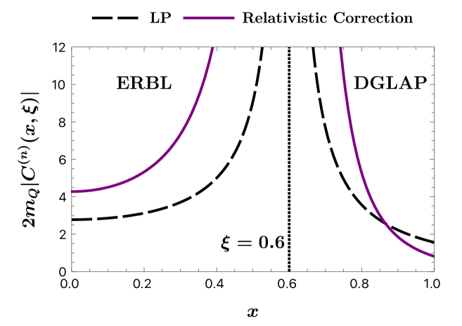
Figure 2: Plot of the absolute value of the matching coefficients in the dimensionless combination $2m_{Q}|C^{(n)}|$ as a function of $x$. We show general photoproduction kinematics with both the ERBL and DGLAP regions for the choice $\xi=0.6$. The LP term $|C^{(0)}(x,\xi)|$ corresponds to the dashed (black) line while the relativistic correction $|C^{(2)}(x,\xi)|$ corresponds to the purple line (Only the purple line in the DGLAP region is negative). Here $\langle v^{2}\rangle=0.22$ which is appropriate for $J/\psi$.

Physically this is the transition point between the DGLAP and ERBL region where one of the gluons is soft. These singularities at the endpoints of the two different kinematic regions are seen in other processes as well. The authors in Cui:2018jha found similar endpoint divergences in exclusive photoproduction of HVM in the high energy limit when calculating higher twist corrections. Within the Soft-Collinear Effective Theory (SCET) framework Bauer:2000ew ; Bauer:2000yr ; Bauer:2001ct ; Bauer:2001yt ; Bauer:2002nz these endpoint divergences have been found in computations of subleading power corrections for various processes Liu:2019oav ; Beneke:2022obx ; Luke:2022ops . The cancellation of the divergences happens between different kinematic regions and can be handled by proper organization of components of the subleading power factorization theorem. For our process we expect an additional soft contribution that is active in the region $x\to\pm\xi$, but we leave the exploration and cancellation of these endpoint divergences for exclusive HVM photoproduction to future work.

On the other hand, for the near-threshold region, one must expand Eq. (23) about $|x|\ll|\xi|$, which gives

$$\mathcal{M}[V]=\frac{4\sqrt{2}\pi g_{e}e_{Q}\alpha_{s}}{3m_{Q}}\left(\frac{\langle\mathcal{O}_{1}(^{3}S_{1})\rangle_{V}}{M_{V}}\right)^{1/2}\left(\varepsilon_{\gamma}^{\perp}\cdot\varepsilon_{V}^{*\perp}\right)\left(1+\frac{7\langle v^{2}\rangle_{V}}{3}\right)G^{(0)}(t,\xi).$$ (24)

The small $x$ expansion circumvents the issue of the endpoint divergence, by expanding in a regime far from the the dangerous pole. In practice only one or a few terms are kept in the expansion, leading to well defined results.

3 Photoproduction cross-section

While we obtained the amplitude in the Ji frame, for easier comparison with previous work we calculate the cross-section in the proton-photon center-of-mass frame. The two frames are related by a rotation and a boost. Under the latter the collinear expansion is invariant while the former introduces a correction of the $O(t/W^{2})$. This again is a kinematic power correction and thus is neglected in our calculation. The differential cross-section is obtained from Eq.(24), and is given by

$$\frac{d\sigma}{dt} =\frac{1}{16\pi(W^{2}-M_{N}^{2})}\frac{1}{2}\sum_{\text{polarization}}|\mathcal{M}|^{2}$$

$$=\frac{\alpha_{\text{EM}}e^{2}_{Q}}{(W^{2}-M_{N}^{2})}\left(\frac{2\pi\alpha_{s}}{3}\right)^{2}\left(\frac{M_{V}\langle O_{1}\rangle_{V}}{2m_{Q}^{4}(1+\langle v^{2}\rangle_{V})}\right)\left(1+\frac{7\langle v^{2}\rangle_{V}}{3}\right)^{2}\frac{1}{2}\sum_{\text{polarization}}\left|G^{(0)}(\xi,t)\right|^{2},$$ (25)

where the sum and averaging is over the polarization of the initial and final proton state. Using the parametrization of the gluon GPD correlator in Eq.(13), the sum/average of the squared moment of GPD has the form

$$\frac{1}{2}\sum_{\text{polarization}}\left|G^{(0)}(\xi,t)\right|^{2} =\frac{1}{\xi^{4}}\Bigg{[}\left(1-\xi^{2}\right)(E_{2}(t,\xi)+H_{2}(t,\xi))^{2}$$

$$-2E_{2}(t,\xi)(E_{2}(t,\xi)+H_{2}(t,\xi))+\left(1-\frac{t}{4M_{N}^{2}}\right)E_{2}(t,\xi)^{2}\Bigg{]}\,.$$ (26)

To compare with GlueX data, we take the physical constants similar to the ones used in Guo:2023pqw , with the proton mass $M_{N}=0.938$ GeV, $J/\psi$ mass $M_{J/\psi}=3.097$ GeV and $\alpha_{s}(\mu=2\,\text{GeV})=0.3$. For the relativistic correction an additional parameter to consider is the charm quark mass which we take to be the 1S mass $m_{c}^{1S}=1.3\,\text{GeV}$ Bernlochner:2020jlt . This gives $\langle v^{2}\rangle_{J/\psi}=0.42$ from the Gremm-Kapustin relation. The other inputs for the cross-section are the nonperturbative matrix elements. The LDME $\langle\mathcal{O}_{1}(^{3}S_{1})\rangle_{J/\psi}$ can be estimated from the leptonic decay rate of $J/\psi$ Eichten:2019hbb

$$\langle\mathcal{O}_{1}(^{3}S_{1})\rangle_{J/\psi}=6|\psi_{1S}(0)|^{2}=\frac{6.5712}{4\pi}\,\text{GeV}^{3}\,.$$ (27)

Finally the gravitational form factors are taken from lattice calculations Pefkou:2021fni with the $t$ dependence in the tripole expansion being

$$A_{g}(t) =\frac{A_{g}(0)}{\left(1-\frac{t}{m_{A}}\right)^{3}}, B_{g}(t) =\frac{B_{g}(0)}{\left(1-\frac{t}{m_{B}}\right)^{3}}, C_{g}(t) =\frac{C_{g}(0)}{\left(1-\frac{t}{m_{C}}\right)^{3}}.$$ (28)

The values for the parameters in the above expression are: $A_{g}(0)=0.429,m_{A}=1.641\,\text{GeV}$, $B_{g}(0)=0.097,m_{B}=4.0\,\text{GeV}$ and $C_{g}(0)=-1.93,m_{C}=1.07\,\text{GeV}$.

Our results for the inclusion of relativistic corrections in the $J/\Psi$ cross-section are shown in Fig. 3.

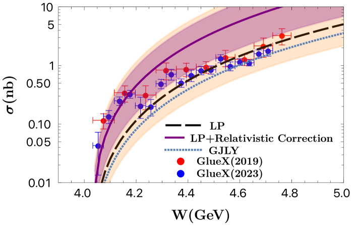
Figure 3: Log plot of the cross-section for $J/\psi$ production, where the threshold region starts from the smallest values of $W$ shown. The leading power (LP) and the relativistic correction to LP obtained from this work are shown in thick (purple) and dashed (black) lines respectively. The dotted line corresponds to LP result from Guo:2023pqw . The yellow and purple shaded regions give two different estimates for the uncertainty from missing power corrections that are of the same size as those computed here.

We also use our results to make a prediction for the Upsilon cross-section in Fig. 4, and give the corresponding parameter values in the figure caption.

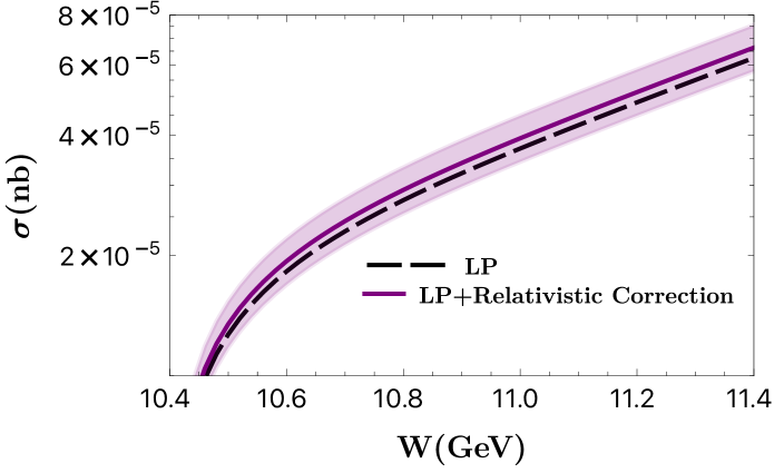
Figure 4: Log plot of the cross-section for $\Upsilon$ production. Mass parameters used for this plot are $M_{\Upsilon}=9.46$ GeV and $m_{b}^{1S}=4.7$ which gives $\langle v^{2}\rangle_{\Upsilon}=0.013$. The purple shaded region gives an estimates for the uncertainty from missing power corrections that are of the same size as those computed here. Here the LDME estimated from leptonic decay is taken to be $\langle\mathcal{O}_{1}(^{3}S_{1})\rangle_{\Upsilon}=\frac{35.1528}{4\pi}\,\text{GeV}^{3}$.

For the $J/\psi$ in Fig. 3, we see that the inclusion of our $v^{2}$ correction gives a substantially improved agreement with data in the threshold limit, taking us from the leading power (black dashed) curve to the solid purple curve which adds relativistic corrections. However, we also note that our estimated uncertainty band is quite large, for which a discussion is warranted. In our predictions the two dominant sources are (i) the uncertainty in the value of the charm quark mass which also leads to uncertainty in the matrix element $\langle v^{2}\rangle$ and (ii) the uncertainty due to excluding power corrections from other sources. The error $\Delta\sigma_{\text{mass}}$ due to (i) is estimated from the error in the 1S mass taken from Bernlochner:2020jlt to be $m_{c}^{1S}=1.3\pm 0.1\,\text{GeV}$. The error $\Delta\sigma_{pow}$ due to (ii) is estimated from the omission of kinematic and subleading GPD corrections which are of similar order as the $v^{2}$ correction. We estimate

$$\Delta\sigma_{\text{pow}}\sim|\mathcal{M}^{(0)}+\mathcal{M}^{(2)}\pm N*\mathcal{M}^{(2)}|^{2}-|\mathcal{M}^{(0)}|^{2}.$$ (29)

Here $\mathcal{M}^{(0)}$ is the leading power amplitude while $\mathcal{M}^{(2)}$ denotes the amplitude purely due to relativistic corrections. Thus $N=0$ gives the difference in the cross-sectional data just from relativistic correction, while $N>0$ with the $\pm$ sign provides an estimate for the upper and lower uncertainty bounds from the missing power corrections. The final uncertainty band is taken to be the root mean square error, $\Delta\sigma=\sqrt{(\Delta\sigma_{\text{pow}})^{2}+(\Delta\sigma_{\text{mass}})^{2}}$. For Fig. 3, the purple band corresponds to the choice $N=0.5$, while the orange band corresponds to $N=1$, which is a more conservative estimate of the error.

The relativistic correction for $J/\psi$ production in Fig. 3 turns out to be quite large relative to the LP result, namely $(100\%\pm 50\%)^{2}$ from determining $\langle v^{2}\rangle$ using $m_{c}=1.3\pm 0.1\,{\rm GeV}$, combined with our estimate for missing power corrections of $(90\%\pm 50\%)^{2}$ (used in the purple band), or even larger $(97\%\pm 97\%)^{2}$ (estimated used in the orange band). Here the square on these estimates translates from the amplitude to cross section level. This big variation in the correction is due to the variation of $\langle v^{2}\rangle_{J/\psi}$ from the charm quark mass. This is reduced in the case of $\Upsilon$ production as can be seen from Fig. 4 because $v^{2}$ is smaller in the bottom system. For the $J/\Psi$ the power corrected result gives good agreement with the low $W$ data compared to LP result. If we were to instead fit to the few points appearing in the threshold region, then we can see from Fig. 4 that we would also obtain a value for $\langle v^{2}\rangle_{V}$ compatible with the Gremm-Kapustin relation in Eq. (21). For the central value of the power corrected cross section, the failure of to agree with data at higher $W$ is likely also related to the breakdown of the moment expansion. Also there is a small difference between the LP results obtained in this work (dashed black curve) and that of Guo:2023pqw (dotted blue curve). This difference comes from the mass which was used in the hard matching coefficient. While here we used $2m_{c}$, the earlier work instead used $M_{J/\psi}$. These coincide with each other only when the relative velocity between the heavy quark-antiquark pair is neglected, that is at LP. However, when adding relativistic effects these differ and for proper inclusion of the results at these different orders one should use the charm quark mass in the hard matching coefficient.

4 Conclusion

We have calculated the relativistic correction to exclusive HVM production in the near-threshold limit in the GPD+NRQCD framework. In general this correction is found to be sizable for $J/\psi$ production in other processes since $v^{2}\sim\alpha_{s}(2m_{c})$ is relatively large. Thus relativistic corrections to $J/\psi$ production are as important as NLO perturbative contributions. We find this to be true in exclusive photoproduction as well. Using inputs from lattice for the nonperturbative matrix elements we compare the relativistically corrected $J/\psi$ production cross-section with that of the GlueX data. At low values of $W$ the subleading corrections lead to better agreement with the experimental results. We also make predictions for $\Upsilon$ production where relativistic corrections are smaller. This provides an important method to test and constrain gluon GPDs at the future EIC collider.

In terms of future work there are two main issues to address. The first is to investigate other sources of power corrections for the complete picture at next-to-leading power. The second is to resolve the issue of endpoint divergence at subleading power in the context of photo/electroproduction away from near-threshold kinematics. We intend to follow up on these topics in future work.

- (1) D. Müller, D. Robaschik, B. Geyer, F.M. Dittes and J. Hořejši, Wave functions, evolution equations and evolution kernels from light ray operators of QCD, Fortsch. Phys. 42 (1994) 101 [hep-ph/9812448].
- (2) A.V. Radyushkin, Nonforward parton distributions, Phys. Rev. D 56 (1997) 5524 [hep-ph/9704207].
- (3) X.-D. Ji, Gauge-Invariant Decomposition of Nucleon Spin, Phys. Rev. Lett. 78 (1997) 610 [hep-ph/9603249].
- (4) P.A. Adderley et al., The Continuous Electron Beam Accelerator Facility at 12 GeV, Phys. Rev. Accel. Beams 27 (2024) 084802 [2408.16880].
- (5) R. Abdul Khalek et al., Science Requirements and Detector Concepts for the Electron-Ion Collider: EIC Yellow Report, Nucl. Phys. A 1026 (2022) 122447 [2103.05419].
- (6) N.N. Nikolaev and B.G. Zakharov, Color transparency and scaling properties of nuclear shadowing in deep inelastic scattering, Z. Phys. C 49 (1991) 607.
- (7) A.H. Mueller, Soft gluons in the infinite momentum wave function and the BFKL pomeron, Nucl. Phys. B 415 (1994) 373.
- (8) M.G. Ryskin, Diffractive electroproduction in LLA QCD, Z. Phys. C 57 (1993) 89.
- (9) S.J. Brodsky, L. Frankfurt, J.F. Gunion, A.H. Mueller and M. Strikman, Diffractive leptoproduction of vector mesons in QCD, Phys. Rev. D 50 (1994) 3134 [hep-ph/9402283].
- (10) E.V. Kuraev, N.N. Nikolaev and B.G. Zakharov, Diffractive vector mesons beyond the s channel helicity conservation, JETP Lett. 68 (1998) 696 [hep-ph/9809539].
- (11) I.P. Ivanov and N.N. Nikolaev, Diffractive S and D wave vector mesons in deep inelastic scattering, JETP Lett. 69 (1999) 294 [hep-ph/9901267].
- (12) I.P. Ivanov and N.N. Nikolaev, Diffractive vector meson production in k(t) factorization approach, Acta Phys. Polon. B 33 (2002) 3517 [hep-ph/0206298].
- (13) D.Y. Ivanov, A. Schafer, L. Szymanowski and G. Krasnikov, Exclusive photoproduction of a heavy vector meson in QCD, Eur. Phys. J. C 34 (2004) 297 [hep-ph/0401131].
- (14) Z.-Q. Chen and C.-F. Qiao, NLO QCD corrections to exclusive electroproduction of quarkonium, Phys. Lett. B 797 (2019) 134816 [1903.00171].
- (15) C.A. Flett, J.A. Gracey, S.P. Jones and T. Teubner, Exclusive heavy vector meson electroproduction to NLO in collinear factorisation, JHEP 08 (2021) 150 [2105.07657].
- (16) J.C. Collins, L. Frankfurt and M. Strikman, Factorization for hard exclusive electroproduction of mesons in QCD, Phys. Rev. D 56 (1997) 2982 [hep-ph/9611433].
- (17) R. Boussarie and Y. Hatta, QCD analysis of near-threshold quarkonium leptoproduction at large photon virtualities, Phys. Rev. D 101 (2020) 114004 [2004.12715].
- (18) Y. Guo, X. Ji and Y. Liu, QCD Analysis of Near-Threshold Photon-Proton Production of Heavy Quarkonium, Phys. Rev. D 103 (2021) 096010 [2103.11506].
- (19) P. Sun, X.-B. Tong and F. Yuan, Near threshold heavy quarkonium photoproduction at large momentum transfer, Phys. Rev. D 105 (2022) 054032 [2111.07034].
- (20) Y. Guo, X. Ji, Y. Liu and J. Yang, Updated analysis of near-threshold heavy quarkonium production for probe of proton’s gluonic gravitational form factors, Phys. Rev. D 108 (2023) 034003 [2305.06992].
- (21) P. Hoodbhoy, Wave function corrections and off forward gluon distributions in diffractive J / psi electroproduction, Phys. Rev. D 56 (1997) 388 [hep-ph/9611207].
- (22) GlueX collaboration, First Measurement of Near-Threshold J/ Exclusive Photoproduction off the Proton, Phys. Rev. Lett. 123 (2019) 072001 [1905.10811].
- (23) GlueX collaboration, Measurement of the J/ photoproduction cross section over the full near-threshold kinematic region, Phys. Rev. C 108 (2023) 025201 [2304.03845].
- (24) W.E. Caswell and G.P. Lepage, Effective Lagrangians for Bound State Problems in QED, QCD, and Other Field Theories, Phys. Lett. B 167 (1986) 437.
- (25) G.T. Bodwin, E. Braaten and G.P. Lepage, Rigorous QCD analysis of inclusive annihilation and production of heavy quarkonium, Phys. Rev. D 51 (1995) 1125 [hep-ph/9407339].
- (26) E. Braaten and T.C. Yuan, Gluon fragmentation into heavy quarkonium, Phys. Rev. Lett. 71 (1993) 1673 [hep-ph/9303205].
- (27) S. Fleming and T. Mehen, Leptoproduction of J / psi, Phys. Rev. D 57 (1998) 1846 [hep-ph/9707365].
- (28) M.E. Luke, A.V. Manohar and I.Z. Rothstein, Renormalization group scaling in nonrelativistic QCD, Phys. Rev. D 61 (2000) 074025 [hep-ph/9910209].
- (29) N. Brambilla, A. Pineda, J. Soto and A. Vairo, Potential NRQCD: An Effective theory for heavy quarkonium, Nucl. Phys. B 566 (2000) 275 [hep-ph/9907240].
- (30) G.T. Bodwin, J. Lee and C. Yu, Resummation of Relativistic Corrections to e+ e- — J/psi + eta(c), Phys. Rev. D 77 (2008) 094018 [0710.0995].
- (31) M. Copeland, S. Fleming, R. Gupta, R. Hodges and T. Mehen, Polarized TMD fragmentation functions for J/ production, Phys. Rev. D 109 (2024) 054017 [2308.08605].
- (32) G.T. Bodwin and A. Petrelli, Order- corrections to -wave quarkonium decay, Phys. Rev. D 66 (2002) 094011 [hep-ph/0205210].
- (33) E. Braaten and J. Lee, Exclusive Double Charmonium Production from Annihilation into a Virtual Photon, Phys. Rev. D 67 (2003) 054007 [hep-ph/0211085].
- (34) M. Gremm and A. Kapustin, Annihilation of S wave quarkonia and the measurement of alpha-s, Phys. Lett. B 407 (1997) 323 [hep-ph/9701353].
- (35) Z.L. Cui, M.C. Hu and J.P. Ma, Gluon GPDs and exclusive photoproduction of quarkonium in forward region, Eur. Phys. J. C 79 (2019) 812 [1804.05293].
- (36) C.W. Bauer, S. Fleming and M.E. Luke, Summing Sudakov logarithms in in effective field theory, Phys. Rev. D63 (2000) 014006 [hep-ph/0005275].
- (37) C.W. Bauer, S. Fleming, D. Pirjol and I.W. Stewart, An Effective field theory for collinear and soft gluons: Heavy to light decays, Phys. Rev. D63 (2001) 114020 [hep-ph/0011336].
- (38) C.W. Bauer and I.W. Stewart, Invariant operators in collinear effective theory, Phys. Lett. B516 (2001) 134 [hep-ph/0107001].
- (39) C.W. Bauer, D. Pirjol and I.W. Stewart, Soft collinear factorization in effective field theory, Phys. Rev. D65 (2002) 054022 [hep-ph/0109045].
- (40) C.W. Bauer, S. Fleming, D. Pirjol, I.Z. Rothstein and I.W. Stewart, Hard scattering factorization from effective field theory, Phys. Rev. D 66 (2002) 014017 [hep-ph/0202088].
- (41) Z.L. Liu and M. Neubert, Factorization at subleading power and endpoint-divergent convolutions in decay, JHEP 04 (2020) 033 [1912.08818].
- (42) M. Beneke, M. Garny, S. Jaskiewicz, J. Strohm, R. Szafron, L. Vernazza et al., Next-to-leading power endpoint factorization and resummation for off-diagonal “gluon” thrust, JHEP 07 (2022) 144 [2205.04479].
- (43) M. Luke, J. Roy and A. Spourdalakis, Factorization at subleading power in deep inelastic scattering in the x→1 limit, Phys. Rev. D 107 (2023) 074023 [2210.02529].
- (44) SIMBA collaboration, Precision Global Determination of the B→Xs Decay Rate, Phys. Rev. Lett. 127 (2021) 102001 [2007.04320].
- (45) E.J. Eichten and C. Quigg, Quarkonium wave functions at the origin: an update, 1904.11542.
- (46) D.A. Pefkou, D.C. Hackett and P.E. Shanahan, Gluon gravitational structure of hadrons of different spin, Phys. Rev. D 105 (2022) 054509 [2107.10368].
- (47) V. Shtabovenko, R. Mertig and F. Orellana, FeynCalc 9.3: New features and improvements, Comput. Phys. Commun. 256 (2020) 107478 [2001.04407].
- (48) V. Shtabovenko, R. Mertig and F. Orellana, New Developments in FeynCalc 9.0, Comput. Phys. Commun. 207 (2016) 432 [1601.01167].
- (49) R. Mertig, M. Bohm and A. Denner, FEYN CALC: Computer algebraic calculation of Feynman amplitudes, Comput. Phys. Commun. 64 (1991) 345.