Probabilistic closed-form formulas for pricing nonlinear payoff variance and volatility derivatives under Schwartz model with time-varying log-return volatility

[Uncaptioned image] Nontawat Bunchak
Department of Statistics
Faculty of Science, Kasetsart University
Bangkok 10900, Thailand
nontawat.bunch@ku.th
&[Uncaptioned image] Udomsak Rakwongwan
Department of Mathematics
Faculty of Science, Kasetsart University
Bangkok 10900, Thailand
udomsak.ra@ku.th
&[Uncaptioned image] Phiraphat Sutthimat
Department of Mathematics
Faculty of Science, Kasetsart University
Bangkok 10900, Thailand
phiraphat.sut@ku.th
Corresponding author
Abstract

This paper presents closed-form analytical formulas for pricing volatility and variance derivatives with nonlinear payoffs under discrete-time observations. The analysis is based on a probabilistic approach assuming that the underlying asset price follows the Schwartz one-factor model, where the volatility of log-returns is time-varying. A difficult challenge in this pricing problem is to solve an analytical formula under the assumption of time-varying log-return volatility, resulting in the realized variance being distributed according to a linear combination of independent noncentral chi-square random variables with weighted parameters. By utilizing the probability density function, we analytically compute the expectation of the square root of the realized variance and derive pricing formulas for volatility swaps. Additionally, we derive analytical pricing formulas for volatility call options. For the payoff function without the square root, we also derive corresponding formulas for variance swaps and variance call options. Additionally, we study the case of constant log-return volatility; simplified pricing formulas are derived and sensitivity with respect to volatility (vega) is analytically studied. Furthermore,we propose simple closed-form approximations for pricing volatility swaps under the Schwartz one-factor model. The accuracy and efficiency of the proposed methods are demonstrated through Monte Carlo simulations, and the impact of price volatility and the number of trading days on fair strike prices of volatility and variance swaps is investigated across various numerical experiments.

Keywords Schwartz one-factor model  \cdot Time-varying volatility  \cdot Noncentral chi-square  \cdot Volatility swaps  \cdot Volatility options  \cdot Vega

1 Introduction

Commodity price volatility has become a focal point for academics, investors, and economists due to its critical role in volatility trading and risk management. Unlike stocks, bonds, and other traditional financial instruments, commodities exhibit exceptionally large price swings around a long-term equilibrium [1], driving demand for volatility-based instruments such as variance and volatility swaps. These forward contracts allow traders to take pure positions on volatility through a simple payoff: at maturity, the long pays a fixed variance strike and receives any realized variance above that level, while the short pays the realized variance and receives the fixed strike. Investor interest in these swaps surged in 1998 following the collapse of Long-Term Capital Management (LTCM) and the ensuing spike in market turbulence; initially dominated by hedge funds selling volatility to dealers [19], the market has since grown into a vibrant arena with extensive research on pricing and hedging these contracts.

Research on variance swap pricing has overwhelmingly focused on equity markets, where a series of foundational studies has established robust valuation and replication methods. Demeterfi et al. [8] demonstrated that, under continuous price paths, variance swaps can be statically replicated using portfolios of vanilla options and that volatility swaps follow by dynamically trading those positions, also deriving an analytical fair-value formula that accounts for realistic volatility skews. Windcliff, Forsyth and Vetzal [35] applied numerical partial integro-differential equation methods to price volatility products and explored delta and delta-gamma hedging strategies for volatility swaps. Javaheri, Wilmott and Haug [13] valued and hedged volatility swaps within a GARCH(1,1) stochastic volatility framework by determining the first two moments of realized variance through a PDE approach and approximating expected realized volatility via Brockhaus and Long’s second-order convexity djustment [2]. Théorét, Zabré and Rostan [33] then provided an analytical solution for pricing volatility swaps under the same GARCH model and applied it to the S&P60 Canada index. Subsequent work by Carr and Madan [15] confirmed exact replication of variance swaps through vanilla options, Ma and Xu [18] incorporated control variate techniques in stochastic volatility settings, Zhu and Lian [37] derived closed-form solutions under Heston’s two-factor model, Rujivan and Zhu [24] offered a simplified analytical approach for discretely sampled variance swaps, Zheng and Kwok [36] extended pricing to generalized swaps with simultaneous jumps in price and variance, Shen and Siu [28] included stochastic interest rates and regime switches, and Chan and Platen [4] developed explicit formulas under the modified constant elasticity of variance model. Despite this extensive equity-focused literature, commodity markets have received little attention; the sole exception is Swishchuk [32], who used the Brockhaus–Long approximation to derive variance and volatility swap formulas for energy assets following a continuous-time GARCH(1,1) process.

In the context of volatility and variance derivatives for commodities, models for stochastic commodity price dynamics differ from those for other asset classes because they explicitly account for the convenience yield and allow for multiple sources of uncertainty. Schwartz [25] introduced three such models. In the first model the log of the spot price follows a mean reverting process around a constant convenience yield. The second model treats the convenience yield itself as stochastic. The third model further extends uncertainty by allowing interest rates to evolve randomly over time. In 2016, Chunhawiksit and Rujivan [6] proposed an analytical closed-form solution for pricing discretely-sampled variance swaps on commodities under the one-factor Schwartz model, defining realized variance via squared percentage returns, validating its financial meaningfulness, and demonstrating substantial computational efficiency gains over Monte Carlo (MC) methods. In the same year, Weraprasertsakun and Rujivan [34] extended this method by deriving a closed-form formula for pricing discretely-sampled variance swaps on commodities, now defining realized variance in terms of squared log returns, showing that their solution produces financially meaningful fair delivery prices throughout the model’s parameter space and dramatically reduces the computational burden compared to MC simulations, thereby offering market practitioners a highly efficient and implementable analytical tool.

However, the results proposed in [6, 34] and also [5, 9, 31] are limited to variance swaps because the closed-form formulas were derived by solving the Feynman–Kac formula to obtain conditional moments of the one-factor Schwartz model, whereas volatility swaps cannot be obtained through conditional moments and instead require half moments of log return. And, of course, the closed-form formula for the half moments of the log returns under the one-factor Schwartz model is not currently available, so a new technique must be introduced to address this issue.

In this paper, we derive closed-form analytical formulas for pricing discretely sampled volatility and variance derivatives under the one-factor Schwartz model with time-varying log-return volatility by expressing the realized variance as a linear combination of independent noncentral chi-square random variables and using their probability density function (PDF) to compute the expectation of its square root. As a result, we obtain explicit pricing formulas for volatility swaps, volatility call options, variance swaps and variance call options (with simplified expressions and analytical vega in the constant-volatility case), propose simple closed-form approximations for volatility swaps, and demonstrate the accuracy and efficiency of our methods through extensive MC simulations.

The remainder of this paper is organized as follows. Section 2 reviews the one-factor Schwartz model. Section 3 introduces variance and volatility swaps. In Section 4, we derive the probability density function of the realized variance and present its conditional moments. Section 5 uses these results to obtain closed-form pricing formulas for volatility and variance swaps and their corresponding options, and provides sensitivity analyzes. Section 7 validates our analytical findings with numerical experiments and discussion. Finally, Section 8 summarizes our contributions and suggests avenues for future research.

2 Schwartz model

In this section we recall Schwartz one-factor model [25] for commodity price dynamics, which we adopt under the risk-neutral probability space (Ω,,(t)t[0,T],)(\Omega,\mathcal{F},(\mathcal{F}_{t})_{t\in[0,T]},\mathbb{Q}) to ensure absence of arbitrage in variance swap pricing. Under \mathbb{Q}, the commodity spot price StS_{t} follows the stochastic differential equation (SDE)

dSt=κ(μlnSt)Stdt+σStdWt,S0>0,t(0,T],\mathrm{d}S_{t}=\kappa(\mu-\ln S_{t})\,S_{t}\,\mathrm{d}t+\sigma\,S_{t}\,\mathrm{d}W_{t},\quad S_{0}>0,\;t\in(0,T], (1)

where κ>0\kappa>0 is the speed of mean reversion to the long-run log-price level μ\mu, σ>0\sigma>0 is the volatility, and (Wt)t[0,T](W_{t})_{t\in[0,T]} is a standard Brownian motion on (Ω,,(t)t[0,T],)(\Omega,\mathcal{F},(\mathcal{F}_{t})_{t\in[0,T]},\mathbb{Q}). Defining the log-price process Xt=lnStX_{t}=\ln S_{t} and applying Itô’s lemma to (1) yields the Ornstein–Uhlenbeck (OU) process

dXt=κ(αXt)dt+σdWt,X0=lnS0,\mathrm{d}X_{t}=\kappa\bigl{(}\alpha-X_{t}\bigr{)}\,\mathrm{d}t+\sigma\,\mathrm{d}W_{t},\quad X_{0}=\ln S_{0}, (2)

where κlnSt\kappa\ln S_{t} is the instantaneous convenience yield at time tt and

α=μσ22κ.\alpha\;=\;\mu\;-\;\frac{\sigma^{2}}{2\,\kappa}\,.

It is important to note that, unlike the original OU process sense, a commodity does not behave like a conventional asset, and its spot price (or equivalently the logarithm of the spot price) serves as the state variable on which contingent claims are written.

3 Variance and volatility swaps

Following the collapse of LTCM in late 1998, when implied stock-index volatility reached unprecedented levels, the market for variance and volatility swaps began to expand. Unlike traditional stock options, these swaps provide pure exposure to future volatility [8] and have attracted investment banks and other financial institutions. Investors use them to speculate on future volatility, to trade the spread between realized and implied volatility or to hedge volatility exposure in other positions. Today, variance and volatility swaps are actively quoted across a broad range of assets such as stock indices, currencies and commodities. In the remainder of this chapter, we provide a comprehensive overview of their definitions, valuation strategies and practical implementations.

In a mathematical context, we define discretely sampled volatility and variance based on the log-returns of the underlying asset price. The primary objective of this paper is to estimate the log-return realized variance, commonly referred to as the realized variance, which is defined as

RVRVd(t1,N,T):=1Ti=2Nln(StiSti1)×1002=AFN1i=2Nln(StiSti1)×1002,RV\equiv RV_{d}(t_{1},N,T):=\frac{1}{T}\sum_{i=2}^{N}\ln{\!\left(\frac{S_{t_{i}}}{S_{t_{i-1}}}\right)}\times 100^{2}=\frac{AF}{N-1}\sum_{i=2}^{N}\ln{\!\left(\frac{S_{t_{i}}}{S_{t_{i-1}}}\right)}\times 100^{2}, (3)

for t1(0,T)t_{1}\in(0,T), where StiS_{t_{i}} is the underlying asset’s closing price at time tit_{i} for the ii-th observation belonging to the total number of observations N2N\geq 2. The term AF=N1T=1ΔtAF=\frac{N-1}{T}=\frac{1}{\Delta t} is the annualization factor, used to standardize the realized variance over the time horizon TT.

3.1 Variance swaps

Under a risk-neutral martingale measure \mathbb{Q}, and assuming that r(t1)r(t_{1}) is the time-varying risk-free interest rate at time t1t_{1}, the value of a variance swap at time t1t_{1} can be expressed as the expected present value of its future payoff:

Vt1,var=et1Tr(s)ds𝔼t1[RVdKwidebarvar]×Lvar,V_{t_{1},\mathrm{var}}=e^{-\int_{t_{1}}^{T}r(s)\,\mathrm{d}s}\,\mathbb{E}_{t_{1}}^{\mathbb{Q}}\big{[}RV_{d}-\widebar{K}_{\mathrm{var}}\big{]}\times L_{\mathrm{var}},

where LvarL_{\mathrm{var}} denotes the notional amount of the swap, measured in dollars per annualized variance point. More specifically, LvarL_{\mathrm{var}} represents the amount received by the holder at maturity for each unit by which the realized variance RVdRV_{d} exceeds the strike Kwidebarvar\widebar{K}_{\mathrm{var}}.

Because there is no upfront cost to enter into a variance swap, we have Vt1,var=0V_{t_{1},\mathrm{var}}=0. Therefore, the fair strike price of a variance swap is given by

Kwidebarvar:=𝔼t1[RVd],\widebar{K}_{\mathrm{var}}:=\mathbb{E}_{t_{1}}^{\mathbb{Q}}\big{[}RV_{d}\big{]}, (4)

where 𝔼t1[X]\mathbb{E}_{t_{1}}^{\mathbb{Q}}[X] denotes the conditional expectation of a random variable XX with respect to the filtration t1\mathcal{F}_{t_{1}} under the risk-neutral martingale measure \mathbb{Q}. Thus, the valuation problem for a variance swap reduces to computing the expected value of the future realized variance in the risk-neutral world.

3.2 Volatility swaps

Similar to the valuation of a variance swap, the value of a volatility swap at time t1t_{1} can be expressed as the expected present value of the future payoff,

Vt1,vol=et1Tr(s)ds𝔼t1[RVdKwidebarvol]×Lvol,V_{t_{1},\mathrm{vol}}=e^{-\int_{t_{1}}^{T}r(s)\,\mathrm{d}s}\,\mathbb{E}_{t_{1}}^{\mathbb{Q}}\big{[}\sqrt{RV_{d}}-\widebar{K}_{\mathrm{vol}}\big{]}\times L_{\mathrm{vol}},

where LvolL_{\mathrm{vol}} is the notional amount of the swap, denominated in dollars per annualized volatility point. Specifically, LvolL_{\mathrm{vol}} represents the amount that the holder of the contract receives at maturity if RVd\sqrt{RV_{d}} exceeds the strike Kwidebarvol\widebar{K}_{\mathrm{vol}} by one unit.

Since there is no upfront cost to enter into a volatility swap, we set Vt1,vol=0V_{t_{1},\mathrm{vol}}=0. Consequently, the fair strike price of a volatility swap is given by

Kwidebarvol:=𝔼t1[RVd].\widebar{K}_{\mathrm{vol}}:=\mathbb{E}_{t_{1}}^{\mathbb{Q}}\big{[}\sqrt{RV_{d}}\big{]}. (5)

3.3 Practical applications

Volatility exhibits several attractive features for trading. First, it rises with risk and uncertainty and tends to increase more after bad news than after good news. Second, it follows a mean reverting process so high volatility levels decrease and low levels increase. Finally, there is a negative correlation between volatility and asset prices so volatility remains high after large downward moves in the market [8]. Variance and volatility swaps allow investors to profit from or hedge against changes in future volatility. For example, a dealer who writes an option can face losses if volatility spikes and the option must be repurchased at a higher price. To transfer this risk, the dealer can enter a volatility swap with a hedge fund. The hedge fund takes the opposite position because it expects volatility to fall and seeks to earn a profit. As the most direct instruments for trading volatility, variance and volatility swaps are central to modern financial markets and will continue to play a key role.

4 The PDF of the realized variance

Consider XtiX_{t_{i}} follows the OU stochastic process (2) with mean 𝔼[Xti]\mathbb{E}\big{[}X_{t_{i}}\big{]} and variance 𝕍𝔸[Xti]\mathbb{VAR}\big{[}X_{t_{i}}\big{]}. Moreover, a covariance of XtiX_{t_{i}} and Xti1X_{t_{i-1}} is denoted by 𝕆𝕍[Xti,Xti1]\mathbb{COV}\big{[}X_{t_{i}},X_{t_{i-1}}\big{]}. Let Zi:=XtiXti1=lnStilnSti1Z_{i}:=X_{t_{i}}-X_{t_{i-1}}=\ln{S_{t_{i}}}-\ln{S_{t_{i-1}}} also known as the log-return. We obtain

Zwidebari=μwidebari+σwidebari2(WtiWti1)𝒩(μwidebari,σwidebari2),\widebar{Z}_{i}=\widebar{\mu}_{i}+\widebar{\sigma}_{i}^{2}\,\big{(}W_{t_{i}}-W_{t_{i-1}}\big{)}\sim\mathcal{N}\big{(}\,\widebar{\mu}_{i},\widebar{\sigma}_{i}^{2}\big{)}, (6)

where

μwidebari:=𝔼[Xti]𝔼[Xti1],\widebar{\mu}_{i}:=\mathbb{E}\big{[}X_{t_{i}}\big{]}-\mathbb{E}\big{[}X_{t_{i-1}}\big{]}, (7)

and

σwidebari2:=𝕍𝔸[Xti]+𝕍𝔸[Xti1]2𝕆𝕍[Xti,Xti1],\widebar{\sigma}_{i}^{2}:=\mathbb{VAR}\big{[}X_{t_{i}}\big{]}+\mathbb{VAR}\big{[}X_{t_{i-1}}\big{]}-2\,\mathbb{COV}\big{[}X_{t_{i}},X_{t_{i-1}}\big{]}, (8)

at time ti(0,T]t_{i}\in(0,T] for i=2,3,,Ni=2,3,\ldots,N. So this means that Zwidebari\widebar{Z}_{i} is a normally distributed random variable with mean μwidebari\widebar{\mu}_{i} and variance σwidebari2\widebar{\sigma}_{i}^{2} for all i=2,3,,Ni=2,3,\ldots,N.

By the definition of the noncentral chi-square random variables, we have

Ywidebari:=(Zwidebariσwidebari)2𝒩𝒞χ12(δwidebari),\widebar{Y}_{i}:=\left(\frac{\widebar{Z}_{i}}{\widebar{\sigma}_{i}}\right)^{2}\sim\mathcal{NC}_{\chi^{2}_{1}}(\widebar{\delta}_{i}), (9)

for all i=2,3,,Ni=2,3,\ldots,N where Yiwidebar\widebar{Y_{i}} is a noncentral chi-square distribution with degrees of freedom νi\nu_{i} and noncentrality parameter δwidebari\widebar{\delta}_{i} where νi=1\nu_{i}=1 then

ν:=i=2Nνi=N1,\nu:=\sum^{N}_{i=2}\nu_{i}=N-1, (10)

and

δwidebari:=(μwidebariσwidebari)2,\widebar{\delta}_{i}:=\left(\frac{\widebar{\mu}_{i}}{\widebar{\sigma}_{i}}\right)^{2}, (11)

for i=2,3,,Ni=2,3,\ldots,N. The log-return realized variance defined in (3) can be shown in terms of a linear combination of noncentral chi-square random variables, by applying (6)–(11), as

RVd(t1,N,T)=i=2NαwidebariYwidebari,RV_{d}(t_{1},N,T)=\sum_{i=2}^{N}\widebar{\alpha}_{i}\widebar{Y}_{i}, (12)

where the weighted parameter can be defined by

αwidebari:=1002Tσwidebari2,\widebar{\alpha}_{i}:=\frac{100^{2}}{T}\widebar{\sigma}^{2}_{i}, (13)

for i=2,3,,Ni=2,3,\ldots,N.

4.1 Laguerre expansions for the PDF of RVdRV_{d}

Over the past several decades, the distribution of linear combinations of noncentral chi-square random variables, or equivalently, quadratic forms in normal random variable vectors, has been the subject of extensive research. The PDFs associated with the distribution have been expressed in various representations, accompanied by many proposed methods for their efficient computation. For instance, in 1961, Shah and Khatri [27] introduced the distribution for the definite case using power series expansions. In 1962, Ruben [22] proposed a representation for the infinite case in terms of chi-squared series. Subsequently, in 1963, Shahe [26] extended their approach to the infinite case and compared their results with those of Ruben. Then, in 1967, Kotz et al. [16] represented the distribution in terms of various expressions including power series expansions, Laguerre series expansions, chi-squared series, and noncentral chi-squared series. Furthermore, in 1977, Davis [7] presented percentage point approximation tables for the distribution under a differential equation approach. To represent the PDF of a linear combination of independent noncentral chi-square random variables with positive weights, as given in (12), one of the most efficient computational methods is developed from the work of Kotz et al. (1967) and Davis (1977), and is represented in terms of Laguerre series expansions proposed by Castaño-Martínez and López-Blázquez in 2005 [3].

For our study, we apply the presented approach by Castaño-Martínez and López-Blázquez [3] to obtain the PDF of RVdRV_{d}, as shown in the following theorem. The generalized Laguerre function is given by the following series representation

𝐋k(a)(x)=m=0(1)m(a+k)!(a+m)!(km)!m!xm,\mathbf{L}^{(a)}_{k}(x)=\sum^{\infty}_{m=0}(-1)^{m}\frac{(a+k)!}{(a+m)!\,(k-m)!\,m!}\,x^{m},

where the parameter a>1a>-1 and the fractional order k(n1,n)k\in(n-1,n) for some nn\in\mathbb{N}.

Theorem 1.

Let y>0y>0. The PDF of RVdRV_{d} written as f𝑤𝑖𝑑𝑒𝑏𝑎𝑟ν\widebar{f}_{\nu}, satisfying

(RVdy)=0yfwidebarν(ζ)dζ,\mathbb{Q}(RV_{d}\leq y)=\int^{y}_{0}\widebar{f}_{\nu}(\zeta)\,\mathrm{d}\zeta,

and can be illustrated as

fwidebarν(y)fwidebarν(βwidebar,μwidebar0)(y):=ey2βwidebaryν21(2βwidebar)ν2k=0Γ(k1)Γ(ν2+k)cwidebark𝐋k(ν21)(νy4βwidebarμwidebar0),\widebar{f}_{\nu}(y)\equiv\widebar{f}_{\nu}^{(\widebar{\beta},\widebar{\mu}_{0})}(y):=\frac{e^{-\frac{y}{2\widebar{\beta}}}y^{\frac{\nu}{2}-1}}{(2\widebar{\beta})^{\frac{\nu}{2}}}\sum^{\infty}_{k=0}\frac{\Gamma(k-1)}{\Gamma\!\left(\frac{\nu}{2}+k\right)}\widebar{c}_{k}\,\mathbf{L}^{\left(\frac{\nu}{2}-1\right)}_{k}\!\!\left(\frac{\nu y}{4\widebar{\beta}\widebar{\mu}_{0}}\right), (14)

with three parameters ν=N1\nu=N-1, β𝑤𝑖𝑑𝑒𝑏𝑎𝑟>0\widebar{\beta}>0, and μ𝑤𝑖𝑑𝑒𝑏𝑎𝑟0>0\widebar{\mu}_{0}>0, where Γ(x)=0tx1etdt\Gamma(x)=\int_{0}^{\infty}t^{x-1}e^{-t}\,\mathrm{d}t is the gamma function. The coefficient c𝑤𝑖𝑑𝑒𝑏𝑎𝑟kc𝑤𝑖𝑑𝑒𝑏𝑎𝑟k(ν,σ𝑤𝑖𝑑𝑒𝑏𝑎𝑟i,μ𝑤𝑖𝑑𝑒𝑏𝑎𝑟i;β𝑤𝑖𝑑𝑒𝑏𝑎𝑟,μ𝑤𝑖𝑑𝑒𝑏𝑎𝑟0)\widebar{c}_{k}\equiv\widebar{c}_{k}\big{(}\nu,\widebar{\sigma}_{i},\widebar{\mu}_{i};\widebar{\beta},\widebar{\mu}_{0}\big{)}, for k=1,2,3,k=1,2,3,\ldots, depends on time-varying log-return volatility σ𝑤𝑖𝑑𝑒𝑏𝑎𝑟i\widebar{\sigma}_{i} and mean μ𝑤𝑖𝑑𝑒𝑏𝑎𝑟i\widebar{\mu}_{i} for i=2,3,,Ni=2,3,\ldots,N, satisfying the following recurrent relation,

cwidebark=1kj=0k1cwidebarjdwidebarkj, for k1,\displaystyle\widebar{c}_{k}=\frac{1}{k}\sum_{j=0}^{k-1}\widebar{c}_{j}\widebar{d}_{k-j},\quad\text{ for }k\geq 1, (15)
cwidebar0=(ν2μwidebar0)ν2i=2N(1+αwidebariβwidebar(ν2μwidebar01))12exp(12i=2Nδwidebariαwidebari(ν2μwidebar0)2βwidebarμwidebar0+αwidebari(ν2μwidebar0)),\displaystyle\widebar{c}_{0}=\left(\frac{\nu}{2\widebar{\mu}_{0}}\right)^{\frac{\nu}{2}}\prod^{N}_{i=2}\left(1+\frac{\widebar{\alpha}_{i}}{\widebar{\beta}}\left(\frac{\nu}{2\widebar{\mu}_{0}}-1\right)\right)^{-\frac{1}{2}}\exp{\left(-\frac{1}{2}\sum^{N}_{i=2}\frac{\widebar{\delta}_{i}\widebar{\alpha}_{i}(\nu-2\widebar{\mu}_{0})}{2\widebar{\beta}\widebar{\mu}_{0}+\widebar{\alpha}_{i}(\nu-2\widebar{\mu}_{0})}\right)}, (16)
dwidebarj=i=2Nνi2(βwidebarαwidebariβwidebarαwidebari(ν2μwidebar01))jjβwidebarν4μwidebar0i=2Nδwidebariαwidebari(βwidebariαwidebari)j1(2μwidebar02βwidebarμwidebar0+αwidebari(ν2μwidebar0))j+1, for j1.\displaystyle\widebar{d}_{j}=\sum^{N}_{i=2}\frac{\nu_{i}}{2}\left(\frac{\widebar{\beta}-\widebar{\alpha}_{i}}{\widebar{\beta}-\widebar{\alpha}_{i}\big{(}\frac{\nu}{2\widebar{\mu}_{0}}-1\big{)}}\right)^{j}-\frac{j\widebar{\beta}\nu}{4\widebar{\mu}_{0}}\sum^{N}_{i=2}\widebar{\delta}_{i}\widebar{\alpha}_{i}(\widebar{\beta}_{i}-\widebar{\alpha}_{i})^{j-1}\left(\frac{2\widebar{\mu}_{0}}{2\widebar{\beta}\widebar{\mu}_{0}+\widebar{\alpha}_{i}(\nu-2\widebar{\mu}_{0})}\right)^{j+1},\quad\text{ for }j\geq 1. (17)
Proof.

We will derive fwidebarν\widebar{f}_{\nu}, i.e. the PDF of RVdRV_{d}, by applying the presented approach by Castaño-Martínez and López-Blázquez [3] in Section 3 as follows.

Firstly, we consider a solution of the mean-reverting OU process (2),

Xti=X0eκti+καeκti0tieκsds+σeκti0tieκsdWt.X_{t_{i}}=X_{0}e^{-\kappa t_{i}}+\kappa\alpha e^{-\kappa t_{i}}\int_{0}^{t_{i}}e^{\kappa s}\,\mathrm{d}s+\sigma e^{-\kappa t_{i}}\int_{0}^{t_{i}}e^{\kappa s}\,\mathrm{d}W_{t}.

We know that XtiX_{t_{i}} is normally distributed with mean

𝔼[Xti]=eκtix0+(1eκti)α\mathbb{E}[X_{t_{i}}]=e^{-\kappa t_{i}}x_{0}+(1-e^{-\kappa t_{i}})\alpha (18)

for given Xt0=x0X_{t_{0}}=x_{0}, and variance

𝕍𝔸[Xti]=σ22κ(1e2κti)\mathbb{VAR}[X_{t_{i}}]=\frac{\sigma^{2}}{2\kappa}(1-e^{-2\kappa t_{i}}) (19)

at time ti(0,T]t_{i}\in(0,T] for i=2,3,,Ni=2,3,\ldots,N. In addition, since XtiX_{t_{i}} and Xti1X_{t_{i-1}} are jointly distributed normal random variables, we then obtain that its covariance can be expressed as

𝕆𝕍[Xti,Xti1]=𝕍𝔸[Xti1]eκΔt,\mathbb{COV}[X_{t_{i}},X_{t_{i-1}}]=\mathbb{VAR}[X_{t_{i-1}}]e^{-\kappa\Delta t}, (20)

where Δt=titi1\Delta t=t_{i}-t_{i-1} (see Franco [11]). According to the second term on RHS of the log-return in (6), the increments (WtjWtj1)𝒩(0,Δt)\big{(}W_{t_{j}}-W_{t_{j-1}}\big{)}\sim\mathcal{N}\big{(}0,\Delta t\big{)} and (WtkWtk1)𝒩(0,Δt)\big{(}W_{t_{k}}-W_{t_{k-1}}\big{)}\sim\mathcal{N}\big{(}0,\Delta t\big{)} for all j,k=2,3,,Nj,k=2,3,\ldots,N and jkj\neq k, are independent by using the property of a standard Brownian motion. Therefore, Zwidebari\widebar{Z}_{i} for i=2,3,,Ni=2,3,\ldots,N, is the sequence of independent and identically distributed (i.i.d) random variables. Thus, a result of a random variable RVdRV_{d} as illustrated in (3) is a linear combination of independent noncentral chi-square random variables with weighted parameters αwidebari>0\widebar{\alpha}_{i}>0 as defined in (12), for i=2,3,,Ni=2,3,\ldots,N.

Secondly, in Section 3 of [3], the constants n,αi,δi,pn,\alpha_{i},\delta_{i},p and the parameters, βi\beta_{i}, and μ0\mu_{0}, are replaced by the following: n=N,αi=αwidebari,δi=δwidebar,p=ν/2,β=βwidebari,μ0=μwidebar0n=N,\alpha_{i}=\widebar{\alpha}_{i},\delta_{i}=\widebar{\delta},p=\nu/2,\beta=\widebar{\beta}_{i},\mu_{0}=\widebar{\mu}_{0}. Consequently, by applying equations (3.2), (3.3), (3.4)a, and (3.4)b in [3], the PDF of RVdRV_{d} can be constructed as shown in (14) where the recurrent coefficient cwidebark\widebar{c}_{k} for k=0,1,2,k=0,1,2,\ldots, can be calculated by using (15) and (16) as well as the coefficient dwidebarj\widebar{d}_{j} for k=1,2,3,k=1,2,3,\ldots, can be calculated by using (17). ∎

4.2 The explicit formula for 𝔼[RVd]\mathbb{E}[RV^{\ell}_{d}]

By utilizing the Laguerre expansion (14) along with some properties of the generalized hypergeometric function

p𝐅q(a1,a2,,ap;b1,b2,,bq;z)=k=0(a1)k(a2)k(ap)k(b1)k(b2)k(bq)kzkk!,_{p}\mathbf{F}_{q}(a_{1},a_{2},\ldots,a_{p};b_{1},b_{2},\ldots,b_{q};z)=\sum_{k=0}^{\infty}\frac{(a_{1})_{k}(a_{2})_{k}\cdots(a_{p})_{k}}{(b_{1})_{k}(b_{2})_{k}\cdots(b_{q})_{k}}\frac{z^{k}}{k!}, (21)

where ()k(\cdot)_{k} denotes the usual Pochhammer symbol [29], the explicit formula for the \ell-th conditional moment of RVdRV_{d} is derived in the following theorem.

Theorem 2.

For any +\ell\in\mathbb{R}_{+}, the raw moment of RVdRV_{d} can be illustrated as

𝔼t1[RVd]=(2βwidebar)k=0(ν2μwidebar0)kΓ(+k+ν2)Γ(k+ν2)𝐅12(k,1kν2;1kν2;2μwidebar0ν)cwidebark,\mathbb{E}^{\mathbb{Q}}_{t_{1}}[RV^{\ell}_{d}]=(2\widebar{\beta})^{\ell}\sum^{\infty}_{k=0}\left(\frac{\nu}{2\widebar{\mu}_{0}}\right)^{k}\frac{\Gamma\!\left(\ell+k+\frac{\nu}{2}\right)}{\Gamma\!\left(k+\frac{\nu}{2}\right)}{{}_{2}\mathbf{F}_{1}}\!\!\left(-k,1-k-\frac{\nu}{2};1-k-\frac{\nu}{2}-\ell;\frac{2\widebar{\mu}_{0}}{\nu}\right)\widebar{c}_{k}, (22)

where the coefficients c𝑤𝑖𝑑𝑒𝑏𝑎𝑟k\widebar{c}_{k}, k=0,1,2,k=0,1,2,\ldots, are chosen according to (15)–(17) and the parameters ν>0\nu>0 and β𝑤𝑖𝑑𝑒𝑏𝑎𝑟>0\widebar{\beta}>0 can be arbitrarily chosen.

Proof.

We define

Fwidebark,:=12βwidebarΓ(k1)Γ(ν2+k)cwidebark𝐋k(ν21)(νy4βwidebarμwidebar0)ey2βwidebaryν21+,\widebar{F}_{k,\ell}:=\frac{1}{2\widebar{\beta}}\frac{\Gamma(k-1)}{\Gamma\!\left(\frac{\nu}{2}+k\right)}\widebar{c}_{k}\,\mathbf{L}^{(\frac{\nu}{2}-1)}_{k}\!\!\left(\frac{\nu y}{4\widebar{\beta}\widebar{\mu}_{0}}\right)\ e^{-\frac{y}{2\widebar{\beta}}}\,y^{\frac{\nu}{2}-1+\ell},

for k=0,1,2,,+k=0,1,2,\ldots,\ell\in\mathbb{R}_{+} where cwidebark\widebar{c}_{k}’s, βwidebar\widebar{\beta}, ν\nu are given in Theorem 1. Employing the symbolic computing package in MATHEMATICA yields

0Fwidebark,(y)dy=(2βwidebar)(ν2μwidebar0)kΓ(+k+ν2)Γ(k+ν2)𝐅12(k,1kν2;1kν2;2μwidebar0ν)cwidebark.\int^{\infty}_{0}\widebar{F}_{k,\ell}(y)\,\mathrm{d}y=(2\widebar{\beta})^{\ell}\left(\frac{\nu}{2\widebar{\mu}_{0}}\right)^{k}\frac{\Gamma\!\left(\ell+k+\frac{\nu}{2}\right)}{\Gamma\!\left(k+\frac{\nu}{2}\right)}{{}_{2}\mathbf{F}_{1}}\!\!\left(-k,1-k-\frac{\nu}{2};1-k-\frac{\nu}{2}-\ell;\frac{2\widebar{\mu}_{0}}{\nu}\right)\widebar{c}_{k}. (23)

According to the uniformly convergent series fwidebarn\widebar{f}_{n} derived in Theorem 1, we obtain that the series k=0Fwidebark,(y)\sum^{\infty}_{k=0}\widebar{F}_{k,\ell}(y) converges uniformly to yfwidebarν(βwidebar,μwidebar0)(y)y^{\ell}\widebar{f}_{\nu}^{(\widebar{\beta},\widebar{\mu}_{0})}(y) i.e.,

yfwidebarν(βwidebar,μwidebar0)(y)=k=0Fwidebark,(y).y^{\ell}\widebar{f}_{\nu}^{(\widebar{\beta},\widebar{\mu}_{0})}(y)=\sum^{\infty}_{k=0}\widebar{F}_{k,\ell}(y). (24)

By using the property of uniformly convergent series and applying (23), (24) yields

𝔼t1[RVd]\displaystyle\mathbb{E}^{\mathbb{Q}}_{t_{1}}\big{[}RV^{\ell}_{d}\big{]} =0yfwidebarν(βwidebar,μwidebar0)(y)dy=k=00Fwidebark,r(y)dy\displaystyle=\int^{\infty}_{0}y^{\ell}\widebar{f}_{\nu}^{(\widebar{\beta},\widebar{\mu}_{0})}(y)\,\mathrm{d}y=\sum^{\infty}_{k=0}\int^{\infty}_{0}\widebar{F}_{k,r}(y)\,\mathrm{d}y
=(2βwidebar)k=0(ν2μwidebar0)kΓ(+k+ν2)Γ(k+ν2)𝐅12(k,1kν2;1kν2;2μwidebar0ν)cwidebark.\displaystyle=(2\widebar{\beta})^{\ell}\sum^{\infty}_{k=0}\left(\frac{\nu}{2\widebar{\mu}_{0}}\right)^{k}\frac{\Gamma\!\left(\ell+k+\frac{\nu}{2}\right)}{\Gamma\!\left(k+\frac{\nu}{2}\right)}{{}_{2}\mathbf{F}_{1}}\!\!\left(-k,1-k-\frac{\nu}{2};1-k-\frac{\nu}{2}-\ell;\frac{2\widebar{\mu}_{0}}{\nu}\right)\widebar{c}_{k}.

This completes the proof. ∎

4.3 Approximates for truncation errors of 𝔼[RVd]\mathbb{E}\big{[}RV^{\ell}_{d}\big{]}

On a computation of 𝔼[RVd]\mathbb{E}\big{[}RV^{\ell}_{d}\big{]} by machine, we have to estimate the error from substituting an infinite sum with a finite sum which is a method known as truncation error. An approximation for the truncation errors of 𝔼[RVd]\mathbb{E}\big{[}RV^{\ell}_{d}\big{]} will be derived in this subsection by applying the approaches stated in Subsection 3.1 of Castaño-Martínez and López-Blázquez (see [3]).

we define

εk1,k2(βwidebar,μwidebar0)(,ν)=(2βwidebar)k=k1+1k2(ν2μwidebar0)kΓ(+k+ν2)Γ(k+ν2)𝐅12(k,1kν2;1kν2;2μwidebar0ν)cwidebark,\varepsilon_{k_{1},k_{2}}^{(\widebar{\beta},\widebar{\mu}_{0})}(\ell,\nu)=(2\widebar{\beta})^{\ell}\sum^{k_{2}}_{k=k_{1}+1}\left(\frac{\nu}{2\widebar{\mu}_{0}}\right)^{k}\frac{\Gamma\!\left(\ell+k+\frac{\nu}{2}\right)}{\Gamma\!\left(k+\frac{\nu}{2}\right)}{{}_{2}\mathbf{F}_{1}}\!\!\left(-k,1-k-\frac{\nu}{2};1-k-\frac{\nu}{2}-\ell;\frac{2\widebar{\mu}_{0}}{\nu}\right)\widebar{c}_{k},

for any ki=0,1,2,k_{i}=0,1,2,\ldots, i=1,2i=1,2, such that k1+1=k2k_{1}+1=k_{2}. Thus, a truncation error of order kk of 𝔼[RVd]\mathbb{E}\big{[}RV^{\ell}_{d}\big{]} is denoted by εk1,k2(βwidebar,μwidebar0)(,ν)\varepsilon_{k_{1},k_{2}}^{(\widebar{\beta},\widebar{\mu}_{0})}(\ell,\nu). To approximate our truncation error, bounds of cwidebark\widebar{c}_{k} for k=0,1,2,k=0,1,2,\ldots, given in (15)–(17), can be derived below.

Lemma 1.

The coefficient c𝑤𝑖𝑑𝑒𝑏𝑎𝑟k\widebar{c}_{k}, k=0,1,2,k=0,1,2,\ldots, satisfies

|cwidebark|ζk(2k+ν2k)k(2k+νν)ν2b0(ν,βwidebar,μwidebar0,δwidebar,ζ),|\widebar{c}_{k}|\leq\zeta^{k}\left(\frac{2k+\nu}{2k}\right)^{k}\left(\frac{2k+\nu}{\nu}\right)^{\frac{\nu}{2}}b_{0}\big{(}\nu,\widebar{\beta},\widebar{\mu}_{0},\widebar{\delta},\zeta\big{)}, (25)

for k=0,1,2,k=0,1,2,\ldots, where ζ=maxi{2,,N}|1α𝑤𝑖𝑑𝑒𝑏𝑎𝑟iβ𝑤𝑖𝑑𝑒𝑏𝑎𝑟1+α𝑤𝑖𝑑𝑒𝑏𝑎𝑟iβ𝑤𝑖𝑑𝑒𝑏𝑎𝑟(ν2μ𝑤𝑖𝑑𝑒𝑏𝑎𝑟01)|\zeta=\max_{i\in\{2,\ldots,N\}}\left|\frac{1-\frac{\widebar{\alpha}_{i}}{\widebar{\beta}}}{1+\frac{\widebar{\alpha}_{i}}{\widebar{\beta}}\left(\frac{\nu}{2\widebar{\mu}_{0}}-1\right)}\right| and

bwidebar0(ν,βwidebar,μwidebar0,δwidebar,ζ)=(ν2μwidebar0)ν2i=2N|1+αwidebariβwidebar(ν2μwidebar01)|12exp(μwidebar0δwidebarνζ14i=2Nδwidebariαwidebari(ν2μwidebar0)βwidebar+αwidebari(ν2μwidebar0)),\widebar{b}_{0}(\nu,\widebar{\beta},\widebar{\mu}_{0},\widebar{\delta},\zeta)=\left(\frac{\nu}{2\widebar{\mu}_{0}}\right)^{\frac{\nu}{2}}\prod^{N}_{i=2}\left|1+\frac{\widebar{\alpha}_{i}}{\widebar{\beta}}\left(\frac{\nu}{2\widebar{\mu}_{0}}-1\right)\right|^{-\frac{1}{2}}\exp{\left(\frac{\widebar{\mu}_{0}\widebar{\delta}}{\nu\zeta}-\frac{1}{4}\sum^{N}_{i=2}\frac{\widebar{\delta}_{i}\widebar{\alpha}_{i}(\nu-2\widebar{\mu}_{0})}{\widebar{\beta}+\widebar{\alpha}_{i}(\nu-2\widebar{\mu}_{0})}\right)}, (26)

where N2N\geq 2 is a positive integer and  δ𝑤𝑖𝑑𝑒𝑏𝑎𝑟=i=2Nδ𝑤𝑖𝑑𝑒𝑏𝑎𝑟i\widebar{\delta}=\sum^{N}_{i=2}\widebar{\delta}_{i}. In addition,

0<ζ<1, if μwidebar0ν4 and βwidebar>12(2ν2μwidebar0)maxi{2,,N}αwidebari.0<\zeta<1,\text{ if }\widebar{\mu}_{0}\geq\frac{\nu}{4}\text{ and }\widebar{\beta}>\frac{1}{2}\left(2-\frac{\nu}{2\widebar{\mu}_{0}}\right)\max_{i\in\{2,\ldots,N\}}\widebar{\alpha}_{i}.
Proof.

We will derive bounds of coefficient cwidebark\widebar{c}_{k}, k=0,1,2,k=0,1,2,\ldots, by applying the presented approach in Lemma 3.1 written by Castaño-Martínez and López-Blázquez (see [3]) as follows. The constants n,αi,δi,pn,\alpha_{i},\delta_{i},p and parameter βi\beta_{i}, and μ0\mu_{0}, are placed by the following: n=N,αi=αwidebari,δi=δwidebari,p=ν/2,β=βwidebari,μ0=μwidebar0n=N,\alpha_{i}=\widebar{\alpha}_{i},\delta_{i}=\widebar{\delta}_{i},p=\nu/2,\beta=\widebar{\beta}_{i},\mu_{0}=\widebar{\mu}_{0}. Then, by applying Lemma 3.1, bounds of coefficient cwidebark\widebar{c}_{k}, k=0,1,2,k=0,1,2,\ldots, can be constructed as shown in (25) where the mention at the end can be derived by using Remark 3.1 given by Castaño-Martínez and López-Blázquez [3]. ∎

According to Lemma 1, we further define

Bk1,k2(βwidebar,μwidebar0)(,ν;ζ):=(2βwidebar)bwidebar0(ν,βwidebar,μwidebar0,δwidebar,ζ)i=k1+1k2pwidebark(,ν,μwidebar0,ζ),B^{(\widebar{\beta},\widebar{\mu}_{0})}_{k_{1},k_{2}}(\ell,\nu;\zeta):=(2\widebar{\beta})^{\ell}\,\widebar{b}_{0}\big{(}\nu,\widebar{\beta},\widebar{\mu}_{0},\widebar{\delta},\zeta\big{)}\sum^{k_{2}}_{i=k_{1}+1}\widebar{p}_{k}\big{(}\ell,\nu,\widebar{\mu}_{0},\zeta\big{)}, (27)

for all ki=0,1,2,k_{i}=0,1,2,\ldots, i=1,2i=1,2, such that k1+1=k2k_{1}+1=k_{2} and ζ>0\zeta>0, where

pwidebark(,ν,μwidebar0,ζ)=(ν2μwidebar0)kΓ(+k+ν2)Γ(k+ν2)|𝐅12(k,1kν2;1kν2;2μwidebar0ν)|(2k+ν2k)k(2k+νν)ν2ζk.\widebar{p}_{k}\big{(}\ell,\nu,\widebar{\mu}_{0},\zeta\big{)}=\left(\frac{\nu}{2\widebar{\mu}_{0}}\right)^{k}\frac{\Gamma\!\left(\ell+k+\frac{\nu}{2}\right)}{\Gamma\!\left(k+\frac{\nu}{2}\right)}\left|{{}_{2}\mathbf{F}_{1}}\!\!\left(-k,1-k-\frac{\nu}{2};1-k-\frac{\nu}{2}-\ell;\frac{2\widebar{\mu}_{0}}{\nu}\right)\right|\left(\frac{2k+\nu}{2k}\right)^{k}\left(\frac{2k+\nu}{\nu}\right)^{\frac{\nu}{2}}\zeta^{k}. (28)

Due to Lemma 1, our bound for truncation error can be derived as the following theorem.

Theorem 3.

Suppose that μ𝑤𝑖𝑑𝑒𝑏𝑎𝑟0ν4\widebar{\mu}_{0}\geq\frac{\nu}{4} and β𝑤𝑖𝑑𝑒𝑏𝑎𝑟>12(2ν2μ𝑤𝑖𝑑𝑒𝑏𝑎𝑟0)maxi{2,,N}α𝑤𝑖𝑑𝑒𝑏𝑎𝑟i\widebar{\beta}>\frac{1}{2}\left(2-\frac{\nu}{2\widebar{\mu}_{0}}\right)\max_{i\in\{2,\ldots,N\}}\widebar{\alpha}_{i}. Then

|εK,(βwidebar,μwidebar0)(,ν)|BK,(βwidebar,μwidebar0)(,ν;ζ),\left|\varepsilon_{K,\infty}^{(\widebar{\beta},\widebar{\mu}_{0})}(\ell,\nu)\right|\leq B^{(\widebar{\beta},\widebar{\mu}_{0})}_{K,\infty}(\ell,\nu;\zeta), (29)

for all K+K\in\mathbb{Z}_{+} and ζ=maxi{2,,N}|1α𝑤𝑖𝑑𝑒𝑏𝑎𝑟iβ𝑤𝑖𝑑𝑒𝑏𝑎𝑟1+α𝑤𝑖𝑑𝑒𝑏𝑎𝑟iβ𝑤𝑖𝑑𝑒𝑏𝑎𝑟(ν2μ𝑤𝑖𝑑𝑒𝑏𝑎𝑟01)|\zeta=\max_{i\in\{2,\ldots,N\}}\left|\frac{1-\frac{\widebar{\alpha}_{i}}{\widebar{\beta}}}{1+\frac{\widebar{\alpha}_{i}}{\widebar{\beta}}\left(\frac{\nu}{2\widebar{\mu}_{0}}-1\right)}\right|.

Proof.

To proceed (29), we utilize (22) and (4.3)–(28). ∎

5 Pricing volatility and variance swaps

By applying Theorem 1 which introduces the PDF of RVdRV_{d}, the fair strike price of volatility and variance swaps, defined in (5) and (4) respectively, can be expressed as

Kwidebarvar=0yfwidebarn(βwidebar,μwidebar0)(y)dy,\widebar{K}_{var}=\int^{\infty}_{0}y\widebar{f}^{(\widebar{\beta},\widebar{\mu}_{0})}_{n}(y)\,\mathrm{d}y, (30)

and

Kwidebarvol=0yfwidebarn(βwidebar,μwidebar0)(y)dy,\widebar{K}_{vol}=\int^{\infty}_{0}y\widebar{f}^{(\widebar{\beta},\widebar{\mu}_{0})}_{n}(\sqrt{y})\,\mathrm{d}y, (31)

respectively.

Although Kwidebarvar\widebar{K}_{var} and Kwidebarvol\widebar{K}_{vol} can be enumerated by using several techniques of numerical integration for both improper integrals above ,(30) and (31), those numerical techniques can lead to complications. To avoid those complications, we simplify the integral into a series of an infinite summation of a generalized hypergeometric function. It is obtained by analyzing the conditional expectation order \ell of RVdRV_{d} known as a raw moment proposed in Theorem 2.

In this section, the fair strike price of a volatility swap and variance swap is derived by setting =1/2\ell=1/2 and =1\ell=1 in (22), respectively. Additionally, we analyze the closed-form formulas for the fair strike price of both swaps in two scenarios, depending on the variance of the log-return: one where the variance changes over time, and another where it remains constant.

5.1 Pricing formulas for volatility and variance swaps: Time-varying log-return volatility

Due to the solution of the SDE in (2), XtiX_{t_{i}}, for i=2,3,,Ni=2,3,\ldots,N, is a normally distributed random variable with time-varying log-return volatility. The difference between XtiX_{t_{i}} and Xti1X_{t_{i-1}}, denoted as Zwidebari\widebar{Z}_{i} in (6), for i=2,3,,Ni=2,3,\ldots,N, also follows a normal distribution with mean given by (18) and variance given by (19). The covariance of this difference is provided by (20).

In this subsection, these time-varying log-return volatility is used to analyze the explicit formulas for volatility and variance swaps, where RVdRV_{d} is considered as a linear combination of independent noncentral chi-square random variables with weighted parameters αwidebari>0\widebar{\alpha}_{i}>0 for i=2,3,,Ni=2,3,\ldots,N.

5.1.1 Volatility swaps price: Kvol1K^{1}_{vol}

By using the probabilistic approach based on the PDF 14, the following theorem provides a closed-form formula for pricing a volatility swap under time-varying log-return volatility. The corresponding result for the case of constant log-return volatility is presented in the subsequent corollary.

Theorem 4.

According to Theorem 2, suppose that μ𝑤𝑖𝑑𝑒𝑏𝑎𝑟0=ν2\widebar{\mu}_{0}=\frac{\nu}{2} and β𝑤𝑖𝑑𝑒𝑏𝑎𝑟>12maxi{2,,N}α𝑤𝑖𝑑𝑒𝑏𝑎𝑟i\widebar{\beta}>\frac{1}{2}\max_{i\in\{2,\ldots,N\}}\widebar{\alpha}_{i}, and we choose =12\ell=\frac{1}{2}. The fair strike price of a volatility swap can be shown as

Kvol11Kwidebarvol1(βwidebar,ν2)(ν,T;σwidebari)=2βwidebark=0(1)kΓ(k+ν+12)Γ(k+ν2)𝐅12(k,1kν2;kν+12;1)cwidebark,K^{1}_{vol_{1}}\equiv\widebar{K}^{\left(\widebar{\beta},\frac{\nu}{2}\right)}_{vol_{1}}(\nu,T;\widebar{\sigma}_{i})=\sqrt{2\widebar{\beta}}\,\sum^{\infty}_{k=0}\left(-1\right)^{k}\frac{\Gamma\!\left(k+\frac{\nu+1}{2}\right)}{\Gamma\!\left(k+\frac{\nu}{2}\right)}{{}_{2}\mathbf{F}_{1}}\!\left(-k,1-k-\frac{\nu}{2};k-\frac{\nu+1}{2};1\right)\widebar{c}_{k}, (32)

where the coefficients c𝑤𝑖𝑑𝑒𝑏𝑎𝑟kc𝑤𝑖𝑑𝑒𝑏𝑎𝑟k(ν,σ𝑤𝑖𝑑𝑒𝑏𝑎𝑟i,μ𝑤𝑖𝑑𝑒𝑏𝑎𝑟i;β𝑤𝑖𝑑𝑒𝑏𝑎𝑟,ν2),k=0,1,2,\widebar{c}_{k}\equiv\widebar{c}_{k}\big{(}\nu,\widebar{\sigma}_{i},\widebar{\mu}_{i};\widebar{\beta},\frac{\nu}{2}\big{)},k=0,1,2,\ldots are calculated by using (15)–(17) and the parameters σ𝑤𝑖𝑑𝑒𝑏𝑎𝑟i,μ𝑤𝑖𝑑𝑒𝑏𝑎𝑟i,ν\widebar{\sigma}_{i},\widebar{\mu}_{i},\nu and α𝑤𝑖𝑑𝑒𝑏𝑎𝑟i\widebar{\alpha}_{i}, i=2,3,,Ni=2,3,\ldots,N, are defined in (7), (8), (10) and (13) respectively.

Proof.

We set μwidebar0=ν/2\widebar{\mu}_{0}=\nu/2, βwidebar>(1/2)maxi{2,,N}αwidebari\widebar{\beta}>(1/2)\max_{i\in\{2,\ldots,N\}}\widebar{\alpha}_{i}, and =1/2\ell=1/2 in (22); we then immediately obtain (32). ∎

Corollary 1.

According to Theorem 4, assume that σ𝑤𝑖𝑑𝑒𝑏𝑎𝑟2=σ𝑤𝑖𝑑𝑒𝑏𝑎𝑟3==σ𝑤𝑖𝑑𝑒𝑏𝑎𝑟N=c\widebar{\sigma}_{2}=\widebar{\sigma}_{3}=\ldots=\widebar{\sigma}_{N}=c, the fair strike price of a volatility swap can be shown as

Kvol21Kwidebarvol2(βwidebar,ν2)(ν,T;c)=2cTΓ(ν+12)Γ(ν2)×100,K^{1}_{vol_{2}}\equiv\widebar{K}^{\left(\widebar{\beta},\frac{\nu}{2}\right)}_{vol_{2}}(\nu,T;c)=\sqrt{\frac{2c}{T}}\,\frac{\Gamma\!\left(\frac{\nu+1}{2}\right)}{\Gamma\!\left(\frac{\nu}{2}\right)}\times 100, (33)

where c>0c>0 can be arbitrarily chosen and ν>0\nu>0 is defined in (10).

Proof.

According to the proof of Theorem 4, since we set σwidebari2=c2\widebar{\sigma}^{2}_{i}=c^{2}, we choose βwidebar=(1002/T)c2\widebar{\beta}=(100^{2}/T)\,c^{2} for all i=2,3,,Ni=2,3,\ldots,N. From (17) and (15), we then obtain that djwidebar=0\widebar{d_{j}}=0 for all j=1,2,3j=1,2,3\ldots, and cwidebark=0\widebar{c}_{k}=0 for all k=1,2,3,k=1,2,3,\ldots. This means that Kwidebarvol21\widebar{K}^{1}_{vol_{2}} exists only if k=0k=0. Obviously, we have ckwidebar=1\widebar{c_{k}}=1 and 𝐅12(k,1kν/2;k(ν+1)/2;1)=1{{}_{2}\mathbf{F}_{1}}\!\left(-k,1-k-\nu/2;k-(\nu+1)/2;1\right)=1 when k=0k=0 for all ν>0\nu>0 by (16) and (21) respectively. Then we immediately obtain (33). ∎

5.1.2 Variance swaps price: Kvar1K^{1}_{var}

Closed-form formulas for pricing variance swaps under both time-varying and constant log-return volatility are presented in the following theorem and corollary.

Theorem 5.

According to Theorem 2, suppose that μ𝑤𝑖𝑑𝑒𝑏𝑎𝑟0=ν2\widebar{\mu}_{0}=\frac{\nu}{2} and β𝑤𝑖𝑑𝑒𝑏𝑎𝑟>12maxi{2,,N}α𝑤𝑖𝑑𝑒𝑏𝑎𝑟i\widebar{\beta}>\frac{1}{2}\max_{i\in\{2,\ldots,N\}}\widebar{\alpha}_{i}, and we choose =1\ell=1. The fair strike price of a variance swap can be shown as

Kvar11Kwidebarvar1(βwidebar,ν2)(ν,T;σwidebari)=2βwidebark=0(1)kΓ(1+k+ν2)Γ(k+ν2)𝐅12(k,1kν2;kν2;1)cwidebark,K^{1}_{var_{1}}\equiv\widebar{K}^{\left(\widebar{\beta},\frac{\nu}{2}\right)}_{var_{1}}(\nu,T;\widebar{\sigma}_{i})=2\widebar{\beta}\sum_{k=0}^{\infty}(-1)^{k}\frac{\Gamma\!\left(1+k+\frac{\nu}{2}\right)}{\Gamma\!\left(k+\frac{\nu}{2}\right)}{{}_{2}\mathbf{F}_{1}}\!\left(-k,1-k-\frac{\nu}{2};-k-\frac{\nu}{2};1\right)\widebar{c}_{k}, (34)

where the coefficients c𝑤𝑖𝑑𝑒𝑏𝑎𝑟kc𝑤𝑖𝑑𝑒𝑏𝑎𝑟k(ν,σ𝑤𝑖𝑑𝑒𝑏𝑎𝑟i,μ𝑤𝑖𝑑𝑒𝑏𝑎𝑟i;β𝑤𝑖𝑑𝑒𝑏𝑎𝑟,ν2),k=0,1,2,\widebar{c}_{k}\equiv\widebar{c}_{k}\big{(}\nu,\widebar{\sigma}_{i},\widebar{\mu}_{i};\widebar{\beta},\frac{\nu}{2}\big{)},k=0,1,2,\ldots are calculated by using (15)–(17) and the parameters σ𝑤𝑖𝑑𝑒𝑏𝑎𝑟i,μ𝑤𝑖𝑑𝑒𝑏𝑎𝑟i,ν\widebar{\sigma}_{i},\widebar{\mu}_{i},\nu and α𝑤𝑖𝑑𝑒𝑏𝑎𝑟i\widebar{\alpha}_{i}, i=2,3,,Ni=2,3,\ldots,N, are defined in (7), (8), (10) and (13) respectively.

Proof.

The equation (34) is acquired by setting (22) as follows: μwidebar0=ν/2\widebar{\mu}_{0}=\nu/2, βwidebar>(1/2)maxi{2,,N}αwidebari\widebar{\beta}>(1/2)\max_{i\in\{2,\ldots,N\}}\widebar{\alpha}_{i}, and =1\ell=1. ∎

Corollary 2.

According to Theorem 4, assume that σ𝑤𝑖𝑑𝑒𝑏𝑎𝑟2=σ𝑤𝑖𝑑𝑒𝑏𝑎𝑟3==σ𝑤𝑖𝑑𝑒𝑏𝑎𝑟N=c\widebar{\sigma}_{2}=\widebar{\sigma}_{3}=\ldots=\widebar{\sigma}_{N}=c, the fair strike price of a variance swap can be shown as

Kvar21Kwidebarvar2(βwidebar,ν2)(ν,T;c)=2c2TΓ(ν2+1)Γ(ν2)×1002,K^{1}_{var_{2}}\equiv\widebar{K}^{\left(\widebar{\beta},\frac{\nu}{2}\right)}_{var_{2}}(\nu,T;c)=\frac{2c^{2}}{T}\frac{\Gamma\!\left(\frac{\nu}{2}+1\right)}{\Gamma\!\left(\frac{\nu}{2}\right)}\times 100^{2}, (35)

where c>0c>0 can be arbitrarily chosen and ν>0\nu>0 is defined in (10).

Proof.

Due to the equation 34, it is easy to obtain (35) by setting all the same parameters and following the presented approach of the proof from the previous Corollary 1. ∎

5.2 Pricing formulas for volatility and variance swaps: Constant log-return volatility

In this subsection, we explore the other explicit solutions of volatility and variance swaps by assuming that the variances of log-returns are set to be the same.

Referring to (6), we assume that Zwidebari\widebar{Z}_{i} is a normally distributed random variable with mean μwidebari\widebar{\mu}_{i} and given variance σwidebari2=σwidebarN2\widebar{\sigma}^{2}_{i}=\widebar{\sigma}^{2}_{N} for i=2,3,,Ni=2,3,\ldots,N, where μwidebari\widebar{\mu}_{i} and σwidebarN\widebar{\sigma}_{N} are computed by (7) and (8) respectively. In other words, for i=2,3,,Ni=2,3,\ldots,N, we choose the variance at i=Ni=N i.e. at time tNt_{N}, to represent the variance of log-returns for all ii-th observations. Since Zwidebari\widebar{Z}_{i} for i=2,3,,Ni=2,3,\ldots,N forms a sequence of i.i.d. random variables as shown in the proof of Theorem 1, we can define a random variable

Wwidebar:=i=2N(ZwidebariσwidebarN)2𝒩𝒞χη(λwidebar),\sqrt{\widebar{W}}:=\sqrt{\sum_{i=2}^{N}\Bigg{(}\frac{{\widebar{Z}_{i}}}{\widebar{\sigma}_{N}}\Bigg{)}^{2}}\sim\mathcal{NC}_{\chi_{\eta}}\!\left(\sqrt{\widebar{\lambda}}\right), (36)

where Wwidebar\sqrt{\widebar{W}} follows the noncentral chi distribution with degrees of freedom η\eta and noncentrality parameter λwidebar\sqrt{\widebar{\lambda}}. Furthermore, a random variable defined by

Wwidebar:=i=2N(ZwidebariσwidebarN)2𝒩𝒞χη2(λwidebar)\widebar{W}:=\sum_{i=2}^{N}\Bigg{(}\frac{{\widebar{Z}_{i}}}{\widebar{\sigma}_{N}}\Bigg{)}^{2}\sim\mathcal{NC}_{\chi^{2}_{\eta}}(\widebar{\lambda}) (37)

is distributed according to the noncentral chi-square distribution with degree η\eta of freedom and noncentrality parameter λwidebar\widebar{\lambda} where

η:=N1\eta:=N-1 (38)

and

λwidebar:=i=2N1μwidebari2σwidebarN2.\widebar{\lambda}:=\sum^{N-1}_{i=2}\frac{\widebar{\mu}^{2}_{i}}{\widebar{\sigma}^{2}_{N}}. (39)

The interesting results are discussed in the following theorems when RVdRV_{d} is a random variable that can be written in terms of a linear combination of independent noncentral chi-square distributions without weighted parameters.

5.2.1 Volatility swaps price: Kvol2K^{2}_{vol}

Since RVd\sqrt{RV_{d}} can be represented in terms of Wwidebar\sqrt{\widebar{W}}, the following theorems provide closed-form formulas for pricing volatility swaps under constant log-return volatility, in the cases where the sum of time-varying log-return means is greater than zero and equal to zero, respectively.

Theorem 6.

Suppose that i=2N1μ𝑤𝑖𝑑𝑒𝑏𝑎𝑟i2>0\displaystyle\sum^{N-1}_{i=2}\widebar{\mu}_{i}^{2}>0 and σ𝑤𝑖𝑑𝑒𝑏𝑎𝑟i2=σ𝑤𝑖𝑑𝑒𝑏𝑎𝑟N2\widebar{\sigma}^{2}_{i}=\widebar{\sigma}^{2}_{N} for all i=2,3,,Ni=2,3,\ldots,N. The fair strike price of a volatility swap can be shown as

Kvol12Kwidebarvol1(η,T;σwidebarN)=σwidebarNπ2T𝐋12(η21)(λwidebar2)×100,K^{2}_{vol_{1}}\equiv\widebar{K}_{vol_{1}}(\eta,T;\widebar{\sigma}_{N})=\widebar{\sigma}_{N}\sqrt{\frac{\pi}{2T}}\,\mathbf{L}^{\big{(}\frac{\eta}{2}-1\big{)}}_{\frac{1}{2}}\!\!\left(-\frac{\widebar{\lambda}}{2}\right)\times 100, (40)

where η>0\eta>0 and λ𝑤𝑖𝑑𝑒𝑏𝑎𝑟>0\widebar{\lambda}>0 are defined in (38) and (39) respectively.

Proof.

Due to (36), we have the following explicit form (see Johnson et al. [14])

𝔼t1[Wwidebar]=π2𝐋12η21(λwidebar2)>0\mathbb{E}_{t_{1}}^{\mathbb{Q}}[\sqrt{\widebar{W}}]=\sqrt{\frac{\pi}{2}}\,\mathbf{L}^{\frac{\eta}{2}-1}_{\frac{1}{2}}\!\!\left(-\frac{\widebar{\lambda}}{2}\right)>0 (41)

where λwidebar\widebar{\lambda} is given in (39). We note that the conditional expectation above is always positive by the property of the explicitly of the Laguerre function (see Mirevki and Boyadiiev [20]). Thus, the realized volatility can be expressed as

RVd=σwidebarNWwidebarT×100.\sqrt{RV_{d}}=\widebar{\sigma}_{N}\sqrt{\frac{\widebar{W}}{T}}\times 100.

In consequence, we get (40) by using (41). ∎

Theorem 7.

Suppose that i=2N1μ𝑤𝑖𝑑𝑒𝑏𝑎𝑟i2=0\displaystyle\sum^{N-1}_{i=2}\widebar{\mu}_{i}^{2}=0 and σ𝑤𝑖𝑑𝑒𝑏𝑎𝑟i2=σ𝑤𝑖𝑑𝑒𝑏𝑎𝑟N2\widebar{\sigma}^{2}_{i}=\widebar{\sigma}^{2}_{N} for all i=2,3,,Ni=2,3,\ldots,N. The fair strike price of a variance swap can be shown as

Kvol22Kwidebarvol2(η,T;σwidebarN)=σwidebarN2TΓ(η+12)Γ(η2)×100,K^{2}_{vol_{2}}\equiv\widebar{K}_{vol_{2}}(\eta,T;\widebar{\sigma}_{N})=\widebar{\sigma}_{N}\sqrt{\frac{2}{T}}\,\frac{\Gamma\!\left(\frac{\eta+1}{2}\right)}{\Gamma\!\left(\frac{\eta}{2}\right)}\times 100, (42)

where η>0\eta>0 is defined in (38).

Proof.

We proceed with the same approach as in the proof of the previous Theorem 6, but now we replace i=2N1μwidebari2=0\sum^{N-1}_{i=2}\widebar{\mu}_{i}^{2}=0. We then obtain λwidebar=0\widebar{\lambda}=0 that

𝐋12(η21)(0)=2πΓ(η+12)Γ(η2),\mathbf{L}^{\big{(}\frac{\eta}{2}-1\big{)}}_{\frac{1}{2}}(0)=\frac{2}{\sqrt{\pi}}\frac{\Gamma\!\left(\frac{\eta+1}{2}\right)}{\Gamma\!\left(\frac{\eta}{2}\right)}, (43)

where 𝐋b(a)(0)=Γ(1+a+b)/(Γ(1+a)Γ(1+b))\mathbf{L}^{(a)}_{b}(0)=\Gamma(1+a+b)/\big{(}\,\Gamma(1+a)\Gamma(1+b)\big{)} with a=1/2a=1/2, b=(η/2)1b=(\eta/2)-1 and Γ(3/2)=π/2\Gamma(3/2)=\sqrt{\pi}/2 (see Mirevki and Boyadiiev [20]). Hence, we obtain (42) by substituting (43) on the RHS of (41). Note that the proof can be completed by considering that Wwidebar\sqrt{\widebar{W}} is distributed according to the central chi distribution with degrees of freedom η\eta when λwidebar=0\widebar{\lambda}=0. ∎

5.2.2 Variance swaps price: Kvar2K^{2}_{var}

The following theorems are closed-form formulas for pricing variance swaps under constant log-return volatility, in the cases where the sum of time-varying log-return means is greater than zero and equal to zero, respectively.

Theorem 8.

Suppose that i=2N1μ𝑤𝑖𝑑𝑒𝑏𝑎𝑟i>0\displaystyle\sum^{N-1}_{i=2}\widebar{\mu}_{i}>0 and σ𝑤𝑖𝑑𝑒𝑏𝑎𝑟i2=σ𝑤𝑖𝑑𝑒𝑏𝑎𝑟N2\widebar{\sigma}^{2}_{i}=\widebar{\sigma}^{2}_{N} for all i=2,3,,Ni=2,3,\ldots,N. The fair strike price of a variance swap can be shown as

Kvar12Kwidebarvar1(η,T;σwidebarN)=σwidebarN2T(η+λwidebar)×1002,K^{2}_{var_{1}}\equiv\widebar{K}_{var_{1}}(\eta,T;\widebar{\sigma}_{N})=\frac{\widebar{\sigma}^{2}_{N}}{T}\,(\eta+\widebar{\lambda})\times 100^{2}, (44)

where η>0\eta>0 and λ𝑤𝑖𝑑𝑒𝑏𝑎𝑟>0\widebar{\lambda}>0 are defined in (38) and (39) respectively.

Proof.

According to (37), the explicit form of conditional expectation of Wwidebar\widebar{W} can be expressed as (see Stuart et al. [30])

𝔼t1[Wwidebar]=η+λwidebar.\mathbb{E}_{t_{1}}^{\mathbb{Q}}[\widebar{W}]=\eta+\widebar{\lambda}. (45)

We can show that the log-return realized variance (12) is simplified by

RVd=σwidebarN2WT×1002.RV_{d}=\frac{\widebar{\sigma}^{2}_{N}W}{T}\times 100^{2}.

We then get (44) by applying (45). ∎

Theorem 9.

Suppose that i=2N1μ𝑤𝑖𝑑𝑒𝑏𝑎𝑟i2=0\displaystyle\sum^{N-1}_{i=2}\widebar{\mu}_{i}^{2}=0 and σ𝑤𝑖𝑑𝑒𝑏𝑎𝑟i2=σ𝑤𝑖𝑑𝑒𝑏𝑎𝑟N2\widebar{\sigma}^{2}_{i}=\widebar{\sigma}^{2}_{N} for all i=2,3,,Ni=2,3,\ldots,N. The fair strike price of a variance swap can be shown as

Kvar22Kwidebarvar2(η,T;σwidebarN)=σwidebarN2Tη×1002,K^{2}_{var_{2}}\equiv\widebar{K}_{var_{2}}(\eta,T;\widebar{\sigma}_{N})=\frac{\widebar{\sigma}^{2}_{N}}{T}\,\eta\times 100^{2}, (46)

where η>0\eta>0 is defined in (38).

Proof.

This proof is similar to the proof of Theorem 8 above. But now, we replace i=2N1μwidebari2=0\sum^{N-1}_{i=2}\widebar{\mu}_{i}^{2}=0 in (39) then λwidebar=0\widebar{\lambda}=0 which (46) is obtained immediately. Note that we can proof directly by considering that Wwidebar\widebar{W} is distributed according to the central chi-square distribution with degrees of freedom η\eta when λwidebar=0\widebar{\lambda}=0. ∎

According to Corollary 1 and 2, if we choose the arbitrary constant c=σwidebarNc=\widebar{\sigma}_{N}, we will get Theorem 6 and 8 respectively. Besides, in [23] written by Rujivan and Rakwongwan, both corollaries can be implied to Theorem 2.3 when c=σ2Δtc=\sigma^{2}\Delta t and ν=N1\nu=N-1, and Theorem 2.7 when c=βwidebarc=\widebar{\beta}, j=2j=2 and ν=N1\nu=N-1, respectively. In their work, the parameters are obtained by using the Black-Scholes model with a time-varying risk-free interest rate.

5.2.3 Vega of Kvol2K^{2}_{vol} and Kvar2K^{2}_{var}

In financial mathematics, to measure the sensitivity of a derivative instrument’s value, we commonly study its partial derivative with respect to the parameter of interest. In this third-level section, we focus on the first-order partial derivative with respect to the price volatility σ\sigma, known as vega, denoted by 𝒱𝐕:=𝐕σ\mathcal{V}_{\mathbf{V}}:=\frac{\partial\mathbf{V}}{\partial\sigma} (see Hull [12]). In other words, vega can be interpreted as the amount of money invested in the derivative instrument per share, indicating the profit or loss resulting from a one percentage point increase or decrease in volatility. We note that an increase in volatility suggests a higher chance of the underlying asset reaching extreme price levels, leading to a corresponding rise in the derivative instrument’s value. Conversely, reduced volatility tends to lower the derivative instrument’s value.

In the following corollaries, exact formulas for vega of volatility and variance swaps, 𝒱Kvol2\mathcal{V}_{K^{2}_{vol}} and 𝒱Kvol2\mathcal{V}_{K^{2}_{vol}}, are produced by using Theorems 69.

Corollary 3.

According to Theorem 6 and 7, we get the following two results:

  1. 1.

    if i=2N1μwidebari2>0\displaystyle\sum^{N-1}_{i=2}\widebar{\mu}_{i}^{2}>0 then

    𝒱Kvol12=1σ(λwidebarσwidebarNπ2T𝐋12η2(λwidebar2)×100+Kwidebarvol12),\mathcal{V}_{K^{2}_{vol_{1}}}=\frac{1}{\sigma}\left(\widebar{\lambda}{\widebar{\sigma}_{N}}\sqrt{\frac{\pi}{2T}}\,\mathbf{L}^{\frac{\eta}{2}}_{-\frac{1}{2}}\!\!\left(-\frac{\widebar{\lambda}}{2}\right)\times 100+\widebar{K}^{2}_{vol_{1}}\right), (47)

    where λwidebar\widebar{\lambda} is defined in (39).

  2. 2.

    if i=2N1μwidebari2=0\displaystyle\sum^{N-1}_{i=2}\widebar{\mu}_{i}^{2}=0 then

    𝒱Kwidebarvol22=Kwidebarvol22σ.\mathcal{V}_{\widebar{K}^{2}_{vol_{2}}}=\frac{\widebar{K}^{2}_{vol_{2}}}{\sigma}. (48)
Proof.

Utilizing (8), (19), and (20), the variance of the log-return at time tNt_{N} can be expressed as

σwidebarN=(σ22κ(1e2κtN)+σ22κ(1e2κtN1)2(σ22κ(1e2κtN1))eκΔt)12=σ(1κ+12κ(2eκ(tN+tN1)2eκ(tNtN1)e2κtNe2κtN1))12.\displaystyle\begin{split}\widebar{\sigma}_{N}&=\left(\frac{\sigma^{2}}{2\kappa}(1-e^{-2\kappa t_{N}})+\frac{\sigma^{2}}{2\kappa}(1-e^{-2\kappa t_{N-1}})-2\left(\frac{\sigma^{2}}{2\kappa}(1-e^{-2\kappa t_{N-1}})\right)e^{-\kappa\Delta t}\right)^{\frac{1}{2}}\\ &=\sigma\left(\frac{1}{\kappa}+\frac{1}{2\kappa}\left(2e^{-\kappa(t_{N}+t_{N-1})}-2e^{-\kappa(t_{N}-t_{N-1})}-e^{-2\kappa t_{N}}-e^{-2\kappa t_{N-1}}\right)\right)^{\frac{1}{2}}.\end{split}

We then obtain its partial derivative as

σwidebarNσ=σwidebarNσ.\frac{\partial\widebar{\sigma}_{N}}{\partial\sigma}=\frac{\widebar{\sigma}_{N}}{\sigma}. (49)

From Theorem 6, we consider the case that i=2N1μwidebari2>0\sum^{N-1}_{i=2}\widebar{\mu}_{i}^{2}>0, we obtain the following partial derivative:

Kvol12σ=π2T(σwidebarNσ(𝐋12(η21)(i=2N1μwidebari22σwidebarN2))+𝐋12(η21)(i=2N1μwidebari22σwidebarN2)(σwidebarNσ))×100=σwidebarNπ2Tσ(𝐋12(η21)(i=2N1μwidebari22σwidebarN2))×100+Kwidebarvol12σ.\displaystyle\begin{split}\frac{\partial K^{2}_{vol_{1}}}{\partial\sigma}&=\sqrt{\frac{\pi}{2T}}\left(\widebar{\sigma}_{N}\frac{\partial}{\partial\sigma}\left(\mathbf{L}^{\left(\frac{\eta}{2}-1\right)}_{\frac{1}{2}}\!\left(-\sum^{N-1}_{i=2}\frac{\widebar{\mu}^{2}_{i}}{2\widebar{\sigma}^{2}_{N}}\right)\right)+\mathbf{L}^{\left(\frac{\eta}{2}-1\right)}_{\frac{1}{2}}\!\left(-\sum^{N-1}_{i=2}\frac{\widebar{\mu}^{2}_{i}}{2\widebar{\sigma}^{2}_{N}}\right)\left(\frac{\partial\widebar{\sigma}_{N}}{\partial\sigma}\right)\right)\times 100\\ &=\widebar{\sigma}_{N}\sqrt{\frac{\pi}{2T}}\frac{\partial}{\partial\sigma}\left(\mathbf{L}^{\left(\frac{\eta}{2}-1\right)}_{\frac{1}{2}}\!\left(-\sum^{N-1}_{i=2}\frac{\widebar{\mu}^{2}_{i}}{2\widebar{\sigma}^{2}_{N}}\right)\right)\times 100+\frac{\widebar{K}^{2}_{vol_{1}}}{\sigma}.\end{split} (50)

By applying the property of the Laguerre function (see Mirevski and Boyadjiev [20]), we get

σ(𝐋12(η21)(i=2N1μwidebari22σwidebarN2))=ddu𝐋12(η21)(u)ddσ(u)=𝐋12η2(u)ddσ(u),\frac{\partial}{\partial\sigma}\left(\mathbf{L}^{\left(\frac{\eta}{2}-1\right)}_{\frac{1}{2}}\left(-\sum^{N-1}_{i=2}\frac{\widebar{\mu}^{2}_{i}}{2\widebar{\sigma}^{2}_{N}}\right)\right)=\frac{\mathrm{d}}{\mathrm{d}\mathrm{u}}\mathbf{L}^{\left(\frac{\eta}{2}-1\right)}_{\frac{1}{2}}\left(\mathrm{-u}\right)\frac{\mathrm{d}}{\mathrm{d}\sigma}(-\mathrm{u})=\mathbf{L}^{\frac{\eta}{2}}_{-\frac{1}{2}}\left(-\mathrm{u}\right)\frac{\mathrm{d}}{\mathrm{d}\sigma}(-\mathrm{u}), (51)

where u=i=2N1μwidebari22σwidebarN2\mathrm{u}=\sum^{N-1}_{i=2}\frac{\widebar{\mu}^{2}_{i}}{2\widebar{\sigma}^{2}_{N}}. Then the derivative of u\mathrm{u} with respect to σwidebarN\widebar{\sigma}_{N} can be found as

ddσ(u)=ddσ(u)=i=2N1μwidebari2σwidebarN3σwidebarNσ=i=2N1μwidebari2σwidebarN2(1σ)=λwidebarσ\frac{\mathrm{d}}{\mathrm{d}\sigma}(-\mathrm{u})=-\frac{\mathrm{d}}{\mathrm{d}\sigma}(\mathrm{u})=\frac{\sum^{N-1}_{i=2}\widebar{\mu}^{2}_{i}}{\widebar{\sigma}^{3}_{N}}\frac{\partial\widebar{\sigma}_{N}}{\partial\sigma}=\frac{\sum^{N-1}_{i=2}\widebar{\mu}^{2}_{i}}{\widebar{\sigma}^{2}_{N}}\left(\frac{1}{\sigma}\right)=\frac{\widebar{\lambda}}{\sigma} (52)

The result shown in (47), is simplified by substituting (52) into (51) and (50). Under the condition that i=2N1μwidebari2=0\sum^{N-1}_{i=2}\widebar{\mu}_{i}^{2}=0, by Theorem 7, it is easy to get that

Kvol22σ=Kvol22σwidebarN(σwidebarNσ)=σwidebarNσ2TΓ(η+12)Γ(η2)×100,\frac{\partial K^{2}_{vol_{2}}}{\partial\sigma}=\frac{\partial K^{2}_{vol_{2}}}{\partial\widebar{\sigma}_{N}}\left(\frac{\partial\widebar{\sigma}_{N}}{\partial\sigma}\right)=\frac{\widebar{\sigma}_{N}}{\sigma}\sqrt{\frac{2}{T}}\frac{\Gamma\!\left(\frac{\eta+1}{2}\right)}{\Gamma\!\left(\frac{\eta}{2}\right)}\times 100,

which implies (48). ∎

Corollary 4.

According to Theorem 8 and 9, we have

νKvarj2=2σwidebarN2σTη×1002=2Kwidebarvar22σ,{\nu}_{K^{2}_{var_{j}}}=\frac{2\widebar{\sigma}^{2}_{N}}{\sigma T}\eta\times 100^{2}=\frac{2\widebar{K}^{2}_{var_{2}}}{\sigma}, (53)

for j=1,2j=1,2 where η\eta is defined in (38).

Proof.

From Theorem 8, let j=1j=1, if i=2N1μwidebari2>0\sum^{N-1}_{i=2}\widebar{\mu}_{i}^{2}>0, we arrive

Kvar12σ=1T(2ησwidebarN(σwidebarNσ)+σwidebarN2(λwidebarσ)+2λwidebarσwidebarN(σwidebarNσ))×1002=2σwidebarN2σT(ηλwidebar+λwidebar)×1002=2σwidebarN2σTη×1002,\displaystyle\begin{split}\frac{\partial K^{2}_{var_{1}}}{\partial\sigma}&=\frac{1}{T}\left(2\eta\widebar{\sigma}_{N}\left(\frac{\partial\widebar{\sigma}_{N}}{\partial\sigma}\right)+\widebar{\sigma}^{2}_{N}\left(\frac{\partial\widebar{\lambda}}{\partial\sigma}\right)+2\widebar{\lambda}\widebar{\sigma}_{N}\left(\frac{\partial\widebar{\sigma}_{N}}{\partial\sigma}\right)\right)\times 100^{2}\\ &=\frac{2\widebar{\sigma}^{2}_{N}}{\sigma T}\left(\eta-\widebar{\lambda}+\widebar{\lambda}\right)\times 100^{2}\\ &=\frac{2\widebar{\sigma}^{2}_{N}}{\sigma T}\eta\times 100^{2},\end{split}

where σwidebarNσ=σwidebarNσ and λwidebarσ=2λwidebarσ\frac{\partial\widebar{\sigma}_{N}}{\partial\sigma}=\frac{\widebar{\sigma}_{N}}{\sigma}\text{\ and \ }\frac{\partial\widebar{\lambda}}{\partial\sigma}=\frac{-2\widebar{\lambda}}{\sigma} can be obtained by using (49) and applying (52) with u=i=2N1μwidebari2σwidebarN2=λwidebar\mathrm{u}=-\sum^{N-1}_{i=2}\frac{\widebar{\mu}^{2}_{i}}{\widebar{\sigma}^{2}_{N}}=-\widebar{\lambda}, respectively.

On the other hand, let j=1j=1, if i=2N1μwidebari2=0\sum^{N-1}_{i=2}\widebar{\mu}_{i}^{2}=0, from Theorem 9, it is trivial to see that this case yields the same result as the case before. We then obtain (53) ∎

In the case where an analytical formula for pricing volatility and variance swaps with time-varying log-return volatility, Theorems 4 and 5 are utilized. Finding a closed-form formula for vega in such cases remains a challenging topic for future work.

6 Pricing volatility and variance options

As indicated in the put-call parity relations described by Hull in [12], this section presents only an analytical formula for pricing volatility and variance options on calls.

A payoff for a volatility call buyer at expiration time TT on [t1,T][t_{1},T] with a KvolcK^{c}_{vol}-strike can be written as

(RVd(t1,N,T)Kvolc)+\big{(}\sqrt{RV_{d}(t_{1},N,T)}-K^{c}_{vol}\big{)}^{+} (54)

and a payoff for a variance call buyer at expiration time TT on [t1,T][t_{1},T] with a KvarcK^{c}_{var}-strike can be written as

(RVd(t1,N,T)Kvarc)+\big{(}RV_{d}(t_{1},N,T)-K^{c}_{var}\big{)}^{+} (55)

for t1[0,T)t_{1}\in[0,T) where RVdRV_{d} is the realized variance given in (3).

Under the risk-neutral martingale measure \mathbb{Q} with respect to filtration t1\mathcal{F}_{t_{1}}, we focus on calculating the conditional expectations of both call option yields given in (54) and (55) above. In particular, volatility and variance calls can be expressed as

Cvol:=et1Tr(s)ds𝔼t1[(RVd(t1,N,T)Kvolc)+],C_{vol}:=e^{-\int_{t_{1}}^{T}r(s)\ \mathrm{d}s}\mathbb{E}_{t_{1}}^{\mathbb{Q}}\big{[}\big{(}\sqrt{RV_{d}(t_{1},N,T)}-K^{c}_{vol}\big{)}^{+}\big{]}, (56)

where KvolcK^{c}_{vol} is a strike volatility call and

Cvar:=et1Tr(s)ds𝔼t1[(RVd(t1,N,T)Kvarc)+],C_{var}:=e^{-\int_{t_{1}}^{T}r(s)\ \mathrm{d}s}\mathbb{E}_{t_{1}}^{\mathbb{Q}}\big{[}\big{(}RV_{d}(t_{1},N,T)-K^{c}_{var}\big{)}^{+}\big{]}, (57)

where KvarcK^{c}_{var} is a strike variance call and r(t)r(t) is a time-varying risk-free interest rate, respectively. The challenge of this part is that we need to compute both expectations on the RHS of calls (56) and (57), given as follows:

𝔼t1[(RVd(t1,N,T)Kvolc)+]=Kvolc(yKvolc) 2yfwidebarn(βwidebar,μwidebar0)(y2)dy,\mathbb{E}_{t_{1}}^{\mathbb{Q}}\big{[}\big{(}\sqrt{RV_{d}(t_{1},N,T)}-K^{c}_{vol}\big{)}^{+}\big{]}=\int_{K^{c}_{vol}}^{\infty}(y-K^{c}_{vol})\,2y\widebar{f}^{(\widebar{\beta},\widebar{\mu}_{0})}_{n}(y^{2})\,\mathrm{d}y, (58)

and

𝔼t1[(RVd(t1,N,T)Kvolc)+]=Kvarc(yKvarc)fwidebarn(βwidebar,μwidebar0)(y)dy,\mathbb{E}_{t_{1}}^{\mathbb{Q}}\big{[}\big{(}RV_{d}(t_{1},N,T)-K^{c}_{vol}\big{)}^{+}\big{]}=\int_{K^{c}_{var}}^{\infty}(y-K^{c}_{var})\widebar{f}^{(\widebar{\beta},\widebar{\mu}_{0})}_{n}(y)\,\mathrm{d}y, (59)

respectively, where fwidebarn(βwidebar,μwidebar0)(y)\widebar{f}^{(\widebar{\beta},\widebar{\mu}_{0})}_{n}(y) is the PDF given in (14) from Theorem 1. To obtain the RHS of (58), we apply a Jacobian transformation, which gives the relation fwidebarn(βwidebar,μwidebar0)(y)=2yfwidebarn(βwidebar,μwidebar0)(y2)\widebar{f}^{(\widebar{\beta},\widebar{\mu}_{0})}_{n}(\sqrt{y})=2y\widebar{f}^{(\widebar{\beta},\widebar{\mu}_{0})}_{n}(y^{2}).

As the same problem with Section 3, to avoid the complication of numerical integration for the improper integral in (59) and (58), both integrals can be expressed as an infinite summation series through a generalized Laguerre expansion derived by Dufresne [10] in Theorem 2.4. The conditional expectations can then be simplified as

𝔼t1[(RVd(t1,N,T)ρK)+]:=KbeKk=0hk(ρ,t1,N,T)𝐋k(a)(K),\displaystyle\mathbb{E}_{t_{1}}^{\mathbb{Q}}\big{[}\,(RV_{d}(t_{1},N,T)^{\rho}-K)^{+}\big{]}:=K^{b}e^{-K}\sum_{k=0}^{\infty}h_{k}(\rho,t_{1},N,T)\,\mathbf{L}_{k}^{(a)}(K), (60)

for ρ=1/2,1\rho=1/2,1 where aa and bb are real numbers satisfying a>2max(b,0)1a>2\max(b,0)-1. The coefficient hk(ρ,t1,N,T)h_{k}(\rho,t_{1},N,T) on the RHS of (60) is defined in terms of a finite summation series of the conditional moment of RVd(t1,N,T)RV_{d}(t_{1},N,T) order ρτj\rho\tau_{j} for j=0,1,2,j=0,1,2,\ldots, as follows:

hk(ρ,t1,N,T):=j=0kk!(1)j𝔼t1[RVd(t1,N,T)ρτj]Γ(j+a+1)j!(kj)!(ρτj1)ρτj,h_{k}(\rho,t_{1},N,T):=\sum_{j=0}^{k}\frac{k!\,(-1)^{j}\,\mathbb{E}_{t_{1}}^{\mathbb{Q}}\big{[}\,RV_{d}(t_{1},N,T)^{\rho\tau_{j}}\big{]}}{\Gamma(j+a+1)\,j!\,(k-j)!\,(\rho\tau_{j}-1)\,\rho\tau_{j}}, (61)

for j=0,1,2,j=0,1,2,\ldots, where ρτj=ab+j+2\rho\tau_{j}=a-b+j+2 where 𝔼t1[RVd(t1,N,T)ρτj]\mathbb{E}_{t_{1}}^{\mathbb{Q}}\big{[}\,RV_{d}(t_{1},N,T)^{\rho\tau_{j}}\big{]} can be specified based on call options’ type. By setting ρ=1/2\rho=1/2, we obtain the coefficient hkh_{k} for the volatility call, and for the variance call, we set ρ=1\rho=1.

In the following subsection, an analytical formula for pricing volatility and variance options is presented in two cases by setting the variance of the log-return: one with time-varying variances and the other with a constant variance.

6.1 Pricing formulas for volatility and variance options: Time-varying log-return volatility

In this subsection, the variances of log-returns are assumed to change over time, similar to the setup introduced in Subsection 5.2. Then, RVd(t1,N,T)RV_{d}(t_{1},N,T) is considered as derived in (12). Its conditional moment can be computed by using Theorem 2 to evaluate the RHS of (61) and complete the coefficient hk(ρ,t1,N,T)h_{k}(\rho,t_{1},N,T).

6.1.1 Volatility call option prices: Cvol1C_{vol}^{1}

By using the PDF (14), the following theorem provides a closed-form formula for pricing a volatility call option under time-varying log-return volatility.

Theorem 10.

Suppose that ρ=12\rho=\frac{1}{2}. The volatility call of a strike KvolcK^{c}_{vol} at time t1t_{1} can be expressed as

Cvol1Cvol(12,t1,N,T)=et1Tr(s)ds(Kvolc)beKvolck=0hk(12,t1,N,T)𝐋k(a)(Kvolc),C_{vol}^{1}\equiv C_{vol}\left(\frac{1}{2},t_{1},N,T\right)=e^{-\int_{t_{1}}^{T}r(s)\,\mathrm{d}s}(K^{c}_{vol})^{b}e^{-K^{c}_{vol}}\sum_{k=0}^{\infty}h_{k}\left(\frac{1}{2},t_{1},N,T\right)\mathbf{L}_{k}^{(a)}(K^{c}_{vol}), (62)

where hk(12,t1,N,T)h_{k}\left(\frac{1}{2},t_{1},N,T\right), k=0,1,2,k=0,1,2,\ldots, are calculated by using (61) with 𝔼t1[RVd(t1,N,T)τj2]\mathbb{E}_{t_{1}}^{\mathbb{Q}}\big{[}\,RV_{d}(t_{1},N,T)^{\frac{\tau_{j}}{2}}\big{]} written in Theorem 2 where τj2=ab+j+2\frac{\tau_{j}}{2}=a-b+j+2 for j=0,1,2,j=0,1,2,\ldots with scalars a,ba,b\in\mathbb{R} satisfying a>2max(b,0)1a>2\max(b,0)-1.

Proof.

A volatility call can be found by using 56 together with its conditional expectation on the RHS can be computed by setting K=KvolcK=K^{c}_{vol} and ρ=1/2\rho=1/2 in (60) with coefficients hkh_{k} for k=0,1,2,k=0,1,2,\ldots, given in (61). To obtain (61), we have =τj/2\ell=\tau_{j}/2 for j=0,1,2,j=0,1,2,\ldots, which is set in (22). We then immediately obtain (62). ∎

6.1.2 Variance call option prices: Cvar1C_{var}^{1}

The following theorem is a closed-form formula for pricing a variance call option under time-varying log-return volatility.

Theorem 11.

Suppose that ρ=1\rho=1. The variance call of a strike KvarcK^{c}_{var} at time t1t_{1} can be expressed as

Cvar1Cvar(1,t1,N,T)=et1Tr(s)ds(Kvarc)beKvarck=0hk(1,t1,N,T)𝐋k(a)(Kvarc),C_{var}^{1}\equiv C_{var}\left(1,t_{1},N,T\right)=e^{-\int_{t_{1}}^{T}r(s)\,\mathrm{d}s}(K^{c}_{var})^{b}e^{-K^{c}_{var}}\sum_{k=0}^{\infty}h_{k}\left(1,t_{1},N,T\right)\mathbf{L}_{k}^{(a)}(K^{c}_{var}), (63)

where hk(1,t1,N,T)h_{k}\left(1,t_{1},N,T\right), k=0,1,2,k=0,1,2,\ldots, are calculated by using (61) with 𝔼t1[RVd(t1,N,T)τj]\mathbb{E}_{t_{1}}^{\mathbb{Q}}\big{[}\,RV_{d}(t_{1},N,T)^{\tau_{j}}\big{]} written in Theorem 2 where τj=ab+j+2\tau_{j}=a-b+j+2 for j=0,1,2,j=0,1,2,\ldots with scalars a,ba,b\in\mathbb{R} satisfying a>2max(b,0)1a>2\max(b,0)-1.

Proof.

We get a variance call by using (57) and we get the conditional expectation on the RHS of (57) by replacing K=KvarcK=K^{c}_{var} and ρ=1\rho=1 in (60). On the RHS of (60), coefficients hkh_{k} for k=0,1,2,k=0,1,2,\ldots, defined in (61), are computed by letting =τj\ell=\tau_{j} for j=0,1,2,j=0,1,2,\ldots, in (22). Hence, we immediately obtain (63). ∎

6.2 Pricing formulas for volatility and variance options: Constant log-return volatility

The interesting results of this subsection are other explicit solutions of volatility and variance call options, obtained by assuming that the variance of log-returns remains the same. Specifically, we set σwidebar22=σwidebar32==σwidebarN2\widebar{\sigma}^{2}_{2}=\widebar{\sigma}^{2}_{3}=\dots=\widebar{\sigma}^{2}_{N}, following the approach introduced in Subsection 5.2. Under this assumption, the realized variance is expressed as a linear combination of independent noncentral chi-square random variables, and its conditional moment is derived below.

Since Wwidebar𝒩𝒞χη2(λwidebar)\widebar{W}\sim\mathcal{NC}_{\chi_{\eta}^{2}}\left(\widebar{\lambda}\right) defined in (37), its conditional moment order \ell, for >0\ell>0, is obtained from Stuart et al. [30] in explicit form as

𝔼t1[Wwidebar]=2eλwidebar2Γ(+η2)Γ(η2)𝐅11(+η2;η2;λwidebar2),\mathbb{E}_{t_{1}}^{\mathbb{Q}}[\widebar{W}^{\ell}]=2^{\ell}e^{\frac{-\widebar{\lambda}}{2}}\,\frac{\Gamma\!\left(\ell+\frac{\eta}{2}\right)}{\Gamma\!\left(\frac{\eta}{2}\right)}\,{{}_{1}}\mathbf{F}_{1}\!\!\left(\ell+\frac{\eta}{2};\frac{\eta}{2};\frac{\widebar{\lambda}}{2}\right), (64)

where degrees of freedom η\eta and noncentrality parameter λwidebar\widebar{\lambda} are given in (38) and (39), respectively. Hence, a conditional moment of RVd(t1,N,T)RV_{d}(t_{1},N,T) order \ell, for >0\ell>0, is defined as

𝔼t1[RVd(t1,N,T)]:=(σwidebarN2T×100)𝔼t1[Wwidebar].\mathbb{E}_{t_{1}}^{\mathbb{Q}}[RV_{d}(t_{1},N,T)^{\ell}]:=\left(\frac{\widebar{\sigma}_{N}^{2}}{T}\times 100\right)^{\ell}\!\mathbb{E}_{t_{1}}^{\mathbb{Q}}\big{[}\,\widebar{W}^{\ell}\big{]}. (65)

For λwidebar=0\widebar{\lambda}=0, Wwidebar\widebar{W} is distributed according to the central chi-square distribution with degrees of freedom η\eta. By using a property of the generalized hypergeometric function (21), it is clear that a conditional moment of RVd(t1,N,T)RV_{d}(t_{1},N,T) order \ell for >0\ell>0, can be simplified as

𝔼t1[RVd(t1,N,T)]:=(2σwidebarN2T×100)Γ(+η2)Γ(η2).\mathbb{E}_{t_{1}}^{\mathbb{Q}}\big{[}\,RV_{d}(t_{1},N,T)^{\ell}\big{]}:=\left(\frac{2\widebar{\sigma}_{N}^{2}}{T}\times 100\right)^{\ell}\frac{\Gamma\!\left(\ell+\frac{\eta}{2}\right)}{\Gamma\!\left(\frac{\eta}{2}\right)}. (66)

6.2.1 Volatility call option prices: Cvol2C_{vol}^{2}

Since RVd(t1,N,T)\sqrt{RV_{d}(t_{1},N,T)} can be represented in terms of Wwidebar\sqrt{\widebar{W}}, the following theorem provides a closed-form formula for pricing a call volatility option under constant log-return volatility by applying (64).

Theorem 12.

Suppose that ρ=12\rho=\frac{1}{2}. The volatility call of a strike KvolcK^{c}_{vol} at time t1t_{1} can be expressed as

Cvol2Cvol(12,t1,N,T)=et1Tr(s)ds(Kvolc)beKvolck=0hk(12,t1,N,T)𝐋k(a)(Kvolc),C_{vol}^{2}\equiv C_{vol}\left(\frac{1}{2},t_{1},N,T\right)=e^{-\int_{t_{1}}^{T}r(s)\,\mathrm{d}s}(K^{c}_{vol})^{b}e^{-K^{c}_{vol}}\sum_{k=0}^{\infty}h_{k}\left(\frac{1}{2},t_{1},N,T\right)\mathbf{L}_{k}^{(a)}(K^{c}_{vol}), (67)

where hk(12,t1,N,T)h_{k}\left(\frac{1}{2},t_{1},N,T\right), k=0,1,2,k=0,1,2,\ldots, are calculated by using (61) with the following two conditions holding:

  1. 1.

    if   i=2N1μwidebari2>0\displaystyle\sum^{N-1}_{i=2}\widebar{\mu}_{i}^{2}>0   then   𝔼t1[RVd(t1,N,T)τj2]\mathbb{E}_{t_{1}}^{\mathbb{Q}}\big{[}\,RV_{d}(t_{1},N,T)^{\frac{\tau_{j}}{2}}\big{]} is calculated by using (66)

  2. 2.

    if   i=2N1μwidebari2=0\displaystyle\sum^{N-1}_{i=2}\widebar{\mu}_{i}^{2}=0   then   𝔼t1[RVd(t1,N,T)τj2]\mathbb{E}_{t_{1}}^{\mathbb{Q}}\big{[}\,RV_{d}(t_{1},N,T)^{\frac{\tau_{j}}{2}}\big{]} is calculated by using (65)

where τj/2=ab+j+2\frac{\tau_{j}}{/}{2}=a-b+j+2 for j=0,1,2,j=0,1,2,\ldots, with scalars a,ba,b\in\mathbb{R} satisfying a>2max(b,0)1a>2\max(b,0)-1.

Proof.

By using (56), we obtain its conditional expectation on the RHS of (56) by setting K=KvolcK=K^{c}_{vol} and ρ=1/2\rho=1/2 in (60) with coefficients hkh_{k} for k=0,1,2,k=0,1,2,\ldots, defined in (61). To obtain (61), if i=2N1μwidebari2>0\sum^{N-1}_{i=2}\widebar{\mu}_{i}^{2}>0, λwidebar>0\widebar{\lambda}>0, then we calculate the conditional moment of RVd(t1,N,T)RV_{d}(t_{1},N,T) of order \ell by setting =τj/2\ell=\tau_{j}/2 for j=0,1,2,j=0,1,2,\ldots, in (65). On the other hand, for the case that i=2N1μwidebari2=0\sum^{N-1}_{i=2}\widebar{\mu}_{i}^{2}=0, which implies λwidebar=0\widebar{\lambda}=0, we calculate it using (66). We then obtain the result in (67). ∎

6.2.2 Variance call option prices: Cvar2C_{var}^{2}

The following theorem is a closed-form formula for pricing a variance call option under constant log-return volatility by applying (64).

Theorem 13.

Suppose that ρ=1\rho=1. The volatility call of a strike KvarcK^{c}_{var} at time t1t_{1} can be expressed as

Cvar2Cvar(12,t1,N,T)=et1Tr(s)ds(Kvarc)beKvolck=0hk(12,t1,N,T)𝐋k(a)(Kvarc),C_{var}^{2}\equiv C_{var}\left(\frac{1}{2},t_{1},N,T\right)=e^{-\int_{t_{1}}^{T}r(s)\,\mathrm{d}s}(K^{c}_{var})^{b}e^{-K^{c}_{vol}}\sum_{k=0}^{\infty}h_{k}\left(\frac{1}{2},t_{1},N,T\right)\mathbf{L}_{k}^{(a)}(K^{c}_{var}), (68)

where hk(1,t1,N,T)h_{k}\left(1,t_{1},N,T\right), k=0,1,2,k=0,1,2,\ldots, are calculated by using (61) with the following two conditions holding:

  1. 1.

    if   i=2N1μwidebari2>0\displaystyle\sum^{N-1}_{i=2}\widebar{\mu}_{i}^{2}>0   then   𝔼t1[RVd(t1,N,T)τj]\mathbb{E}_{t_{1}}^{\mathbb{Q}}\big{[}\,RV_{d}(t_{1},N,T)^{\tau_{j}}\big{]}   is calculated by using (65),

  2. 2.

    if   i=2N1μwidebari2=0\displaystyle\sum^{N-1}_{i=2}\widebar{\mu}_{i}^{2}=0   then   𝔼t1[RVd(t1,N,T)τj]\mathbb{E}_{t_{1}}^{\mathbb{Q}}\big{[}\,RV_{d}(t_{1},N,T)^{\tau_{j}}\big{]} is calculated by using (66),

where τj=ab+j+2\tau_{j}=a-b+j+2 for j=0,1,2,j=0,1,2,\ldots, with scalars a,ba,b\in\mathbb{R} satisfying a>2max(b,0)1a>2\max(b,0)-1.

Proof.

We get a variance call by using (57) and its conditional expectation on the RHS of (57) by setting K=KvarcK=K^{c}_{var} and ρ=1\rho=1 in (60) with coefficients hkh_{k} for k=0,1,2,k=0,1,2,\ldots, defined in (61). To obtain (61), we proceed with the same approach in the proof of the previous Theorem 12. But now we let =τj\ell=\tau_{j}. We then obtain the result in (68). ∎

6.2.3 Vega of Cvol2C_{vol}^{2} and Cvar2C_{var}^{2}

To obtain vega of call options presented in Theorems 12 and 13, we focus on its partial derivative on the RHS with respect to σ\sigma. We have that the parameter σ\sigma appears only in σwidebarN\widebar{\sigma}_{N}, where σwidebarN\widebar{\sigma}_{N} is an argument in 𝔼t1[RVd(t1,N,T)]\mathbb{E}_{t_{1}}^{\mathbb{Q}}\big{[}\,RV_{d}(t_{1},N,T)^{\ell}\big{]}, as defined in Subsection 6.2. For a given =ρτj\ell=\rho\tau_{j} for ρ=1/2,1\rho=1/2,1 and j=0,1,2,j=0,1,2,\ldots, we have coefficients hkh_{k} for k=0,1,2,k=0,1,2,\ldots, as defined in (61). Then, the partial derivatives of Cvol2C^{2}_{vol} and Cvar2C^{2}_{var} can be expressed as an infinite summation series of hkh^{\prime}_{k}, which hkh^{\prime}_{k} is defined as

hk(ρ,t1,N,T):=σhk(ρ,t1,N,T)=j=0kk!(1)jσ𝔼t1[RVd(t1,N,T)ρτj]Γ(j+a+1)j!(kj)!(ρτj1)ρτj.h^{\prime}_{k}(\rho,t_{1},N,T):=\frac{\partial}{\partial\sigma}h_{k}(\rho,t_{1},N,T)=\sum_{j=0}^{k}\frac{k!\,(-1)^{j}\,\frac{\partial}{\partial\sigma}\mathbb{E}_{t_{1}}^{\mathbb{Q}}\big{[}\,RV_{d}(t_{1},N,T)^{\rho\tau_{j}}\big{]}}{\Gamma(j+a+1)\,j!\,(k-j)!\,(\rho\tau_{j}-1)\,\rho\tau_{j}}. (69)

In the following theorems, we present σ𝔼t1[RVd(t1,N,T)]\frac{\partial}{\partial\sigma}\mathbb{E}_{t_{1}}^{\mathbb{Q}}\big{[}\,RV_{d}(t_{1},N,T)^{\ell}\big{]} for two cases, characterized by the value of λwidebar\widebar{\lambda}.

Theorem 14.

According to (65), if  i=2N1μ𝑤𝑖𝑑𝑒𝑏𝑎𝑟i2>0\displaystyle\sum^{N-1}_{i=2}\widebar{\mu}_{i}^{2}>0 , then the partial derivative of the conditional moment of RVd(t1,N,T)RV_{d}(t_{1},N,T) order \ell for >0\ell>0, is defined as

σ𝔼t1[RVd(t1,N,T)]=eλwidebar2σ(2σwidebarN2T×100)Γ(+η2)Γ(η2)[(λwidebar+2)𝐅11(+η2;η2;λwidebar2)λwidebar(+η2)1(η2)1𝐅11(1++η2;1+η2;λwidebar2)]=(λwidebar+2)σ𝔼t1[RVd(t1,N,T)](2σwidebarN2T×100)λwidebareλwidebar2σΓ(1++η2)Γ(1+η2)𝐅11(1++η2;1+η2;λwidebar2).\displaystyle\begin{split}&\frac{\partial}{\partial\sigma}\mathbb{E}_{t_{1}}^{\mathbb{Q}}\big{[}\,RV_{d}(t_{1},N,T)^{\ell}\big{]}\\ &=\frac{e^{\frac{-\widebar{\lambda}}{2}}}{\sigma}\left(\frac{2\widebar{\sigma}_{N}^{2}}{T}\times 100\right)^{\ell}\frac{\Gamma\!\left(\ell+\frac{\eta}{2}\right)}{\Gamma\!\left(\frac{\eta}{2}\right)}\left[\left(\widebar{\lambda}+2\ell\right){{}_{1}}\mathbf{F}_{1}\!\!\left(\ell+\frac{\eta}{2};\frac{\eta}{2};\frac{\widebar{\lambda}}{2}\right)-\widebar{\lambda}\frac{\left(\ell+\frac{\eta}{2}\right)_{1}}{\left(\frac{\eta}{2}\right)_{1}}{{}_{1}}\mathbf{F}_{1}\!\!\left(1+\ell+\frac{\eta}{2};1+\frac{\eta}{2};\frac{\widebar{\lambda}}{2}\right)\right]\\ &=\frac{\left(\widebar{\lambda}+2\ell\right)}{\sigma}\mathbb{E}_{t_{1}}^{\mathbb{Q}}\big{[}\,RV_{d}(t_{1},N,T)^{\ell}\big{]}-\left(\frac{2\widebar{\sigma}_{N}^{2}}{T}\times 100\right)^{\ell}\frac{\widebar{\lambda}\,e^{\frac{-\widebar{\lambda}}{2}}}{\sigma}\frac{\Gamma\!\left(1+\ell+\frac{\eta}{2}\right)}{\Gamma\!\left(1+\frac{\eta}{2}\right)}{{}_{1}}\mathbf{F}_{1}\!\!\left(1+\ell+\frac{\eta}{2};1+\frac{\eta}{2};\frac{\widebar{\lambda}}{2}\right).\end{split} (70)
Proof.

Suppose that i=2N1μwidebari2>0\sum^{N-1}_{i=2}\widebar{\mu}_{i}^{2}>0. Then, there exists λwidebar>0\widebar{\lambda}>0 such that the partial derivative of the conditional moment of order \ell, given in (65), can be expressed as

σ𝔼t1[RVd(t1,N,T)]=(2T×100)Γ(+η2)Γ(η2)[σwidebarN2eλwidebar2σ𝐅11(+η2;η2;λwidebar2)+𝐅11(+η2;η2;λwidebar2)σ(σwidebarN2eλwidebar2)].\displaystyle\begin{split}&\frac{\partial}{\partial\sigma}\mathbb{E}_{t_{1}}^{\mathbb{Q}}\big{[}\,RV_{d}(t_{1},N,T)^{\ell}\big{]}\\ &=\left(\frac{2}{T}\times 100\right)^{\ell}\frac{\Gamma\!\left(\ell+\frac{\eta}{2}\right)}{\Gamma\!\left(\frac{\eta}{2}\right)}\left[\widebar{\sigma}_{N}^{2\ell}\,e^{\frac{-\widebar{\lambda}}{2}}\frac{\partial}{\partial\sigma}{{}_{1}}\mathbf{F}_{1}\!\!\left(\ell+\frac{\eta}{2};\frac{\eta}{2};\frac{\widebar{\lambda}}{2}\right)+{{}_{1}}\mathbf{F}_{1}\!\!\left(\ell+\frac{\eta}{2};\frac{\eta}{2};\frac{\widebar{\lambda}}{2}\right)\frac{\partial}{\partial\sigma}\left(\widebar{\sigma}_{N}^{2\ell}\,e^{\frac{-\widebar{\lambda}}{2}}\right)\right].\end{split} (71)

From the above equation (71)), firstly, we consider the partial derivative of the hypergeometric function, by using its differentiation formula, see [21, Chapter 13], we have

σ𝐅11(+η2;η2;λwidebar2)=σ𝐅11(+η2;η2;i=2N1μwidebari22σwidebarN2)=σ𝐅11(+η2;η2;u)dudσ=(+η2)1(η2)1𝐅11(1++η2;1+η2;u)dudσ,\displaystyle\begin{split}\frac{\partial}{\partial\sigma}{{}_{1}}\mathbf{F}_{1}\!\!\left(\ell+\frac{\eta}{2};\frac{\eta}{2};\frac{\widebar{\lambda}}{2}\right)&=\frac{\partial}{\partial\sigma}{{}_{1}}\mathbf{F}_{1}\!\!\left(\ell+\frac{\eta}{2};\frac{\eta}{2};\sum^{N-1}_{i=2}\frac{\widebar{\mu}^{2}_{i}}{2\widebar{\sigma}^{2}_{N}}\right)\\ &=\frac{\partial}{\partial\sigma}{{}_{1}}\mathbf{F}_{1}\!\!\left(\ell+\frac{\eta}{2};\frac{\eta}{2};\mathrm{u}\right)\frac{\mathrm{d}\mathrm{u}}{\mathrm{d}\sigma}\\ &=\frac{\left(\ell+\frac{\eta}{2}\right)_{1}}{\left(\frac{\eta}{2}\right)_{1}}{{}_{1}}\mathbf{F}_{1}\!\!\left(1+\ell+\frac{\eta}{2};1+\frac{\eta}{2};\mathrm{u}\right)\frac{\mathrm{d}\mathrm{u}}{\mathrm{d}\sigma},\end{split} (72)

where u=i=2N1μwidebari22σwidebarN2\mathrm{u}=\sum^{N-1}_{i=2}\frac{\widebar{\mu}^{2}_{i}}{2\widebar{\sigma}^{2}_{N}}. By applying (52), we get dudσ=λwidebarσ\frac{\mathrm{d}\mathrm{u}}{\mathrm{d}\sigma}=-\frac{\widebar{\lambda}}{\sigma}. Secondly, we consider the partial derivative of the second term on the RHS of (71), we have

σ(σwidebarN2eλwidebar2)=σwidebarN2(σeλwidebar2)+eλwidebar2(σσwidebarN2),\frac{\partial}{\partial\sigma}\left(\widebar{\sigma}_{N}^{2\ell}e^{\frac{-\widebar{\lambda}}{2}}\right)=\widebar{\sigma}_{N}^{2\ell}\left(\frac{\partial}{\partial\sigma}e^{\frac{-\widebar{\lambda}}{2}}\right)+e^{\frac{-\widebar{\lambda}}{2}}\left(\frac{\partial}{\partial\sigma}\widebar{\sigma}_{N}^{2\ell}\right), (73)

where

σeλwidebar2=σexp(i=2N1μwidebari22σwidebarN2)=σeu=euddσ(u)=λwidebarσeλwidebar2,\frac{\partial}{\partial\sigma}e^{\frac{-\widebar{\lambda}}{2}}=\frac{\partial}{\partial\sigma}\exp{\left(-\sum^{N-1}_{i=2}\frac{\widebar{\mu}^{2}_{i}}{2\widebar{\sigma}^{2}_{N}}\right)}=\frac{\partial}{\partial\sigma}e^{-\mathrm{u}}=e^{-\mathrm{u}}\frac{\mathrm{d}}{\mathrm{d}\sigma}(\mathrm{-u})=\frac{\widebar{\lambda}}{\sigma}e^{\frac{-\widebar{\lambda}}{2}}, (74)

where ddσ(u)=λwidebarσ\frac{\mathrm{d}}{\mathrm{d}\sigma}(\mathrm{-u})=\frac{\widebar{\lambda}}{\sigma} is derived in (52), and

σσwidebarN2=2σwidebarN21(σwidebarNσ)=2σwidebarN2σ,\frac{\partial}{\partial\sigma}\widebar{\sigma}_{N}^{2\ell}=2\ell\,\widebar{\sigma}_{N}^{2\ell-1}\left(\frac{\partial\widebar{\sigma}_{N}}{\partial\sigma}\right)=\frac{2\ell\,\widebar{\sigma}_{N}^{2\ell}}{\sigma}, (75)

where σwidebarNσ=σwidebarNσ\frac{\partial\widebar{\sigma}_{N}}{\partial\sigma}=\frac{\widebar{\sigma}_{N}}{\sigma} is derived in (49). Thus, the result (70) can be simplified by substituting (74) and ((75)) into (73) which (72) and (73) are substituted into (71). ∎

Theorem 15.

According to (65), if  i=2N1μ𝑤𝑖𝑑𝑒𝑏𝑎𝑟i2=0\displaystyle\sum^{N-1}_{i=2}\widebar{\mu}_{i}^{2}=0, then the partial derivative of the conditional moment of RVd(t1,N,T)RV_{d}(t_{1},N,T) order \ell for >0\ell>0 is defined as

σ𝔼t1[RVd(t1,N,T)]=2σ(2σwidebarN2T×100)Γ(+η2)Γ(η2)=2σ𝔼t1[RVd(t1,N,T)].\frac{\partial}{\partial\sigma}\mathbb{E}_{t_{1}}^{\mathbb{Q}}\big{[}\,RV_{d}(t_{1},N,T)^{\ell}\big{]}=\frac{2\ell}{\sigma}\left(\frac{2\widebar{\sigma}_{N}^{2}}{T}\times 100\right)^{\ell}\frac{\Gamma\!\left(\ell+\frac{\eta}{2}\right)}{\Gamma\!\left(\frac{\eta}{2}\right)}=\frac{2\ell}{\sigma}\mathbb{E}_{t_{1}}^{\mathbb{Q}}\big{[}\,RV_{d}(t_{1},N,T)^{\ell}\big{]}. (76)
Proof.

Suppose that i=2N1μwidebari2=0\sum^{N-1}_{i=2}\widebar{\mu}_{i}^{2}=0, then λwidebar=0\widebar{\lambda}=0. From the conditional moment given in (66), it is easy to obtain its partial derivative that

σ𝔼t1[RVd(t1,N,T)]=(2T×100)Γ(+η2)Γ(η2)σσwidebarN2.\frac{\partial}{\partial\sigma}\mathbb{E}_{t_{1}}^{\mathbb{Q}}\big{[}\,RV_{d}(t_{1},N,T)^{\ell}\big{]}=\left(\frac{2}{T}\times 100\right)^{\ell}\frac{\Gamma\!\left(\ell+\frac{\eta}{2}\right)}{\Gamma\!\left(\frac{\eta}{2}\right)}\frac{\partial}{\partial\sigma}\widebar{\sigma}_{N}^{2\ell}.

By substituting σσwidebarN2=2σwidebarN2σ\frac{\partial}{\partial\sigma}\widebar{\sigma}_{N}^{2\ell}=\frac{2\ell\widebar{\sigma}_{N}^{2\ell}}{\sigma}, as derived in (75) from the proof of the previous Theorem 14, we immediately obtain (76). ∎

According to vega defined in the third-level Section 5.2.3, the derivative instruments are considered as volatility and variance call options. In the following corollaries, exact formulas for vega of volatility and variance call options, 𝒱Cvol2\mathcal{V}_{C^{2}_{vol}} and 𝒱Cvol2\mathcal{V}_{C^{2}_{vol}}, are derived by using Theorems 12 and 13, respectively.

Corollary 5.

According to Theorem 12, we have

𝒱Cvol2=et1Tr(s)ds(Kvolc)beKvolck=0hk(12,t1,N,T)𝐋k(a)(Kvolc),\mathcal{V}_{C^{2}_{vol}}=e^{-\int_{t_{1}}^{T}r(s)\,\mathrm{d}s}(K^{c}_{vol})^{b}e^{-K^{c}_{vol}}\sum_{k=0}^{\infty}h^{\prime}_{k}\!\left(\frac{1}{2},t_{1},N,T\right)\mathbf{L}_{k}^{(a)}(K^{c}_{vol}), (77)

where hk(12,t1,N,T)h^{\prime}_{k}\left(\frac{1}{2},t_{1},N,T\right), k=0,1,2,k=0,1,2,\ldots, are calculated by using (69) with the following two conditions holding:

  1. 1.

    if   i=2N1μwidebari2>0\displaystyle\sum^{N-1}_{i=2}\widebar{\mu}_{i}^{2}>0   then   σ𝔼t1[RVd(t1,N,T)τj2]\frac{\partial}{\partial\sigma}\mathbb{E}_{t_{1}}^{\mathbb{Q}}\big{[}\,RV_{d}(t_{1},N,T)^{\frac{\tau_{j}}{2}}\big{]}   is calculated by using Theorem 14

  2. 2.

    if   i=2N1μwidebari2=0\displaystyle\sum^{N-1}_{i=2}\widebar{\mu}_{i}^{2}=0    then   σ𝔼t1[RVd(t1,N,T)τj2]\frac{\partial}{\partial\sigma}\mathbb{E}_{t_{1}}^{\mathbb{Q}}\big{[}\,RV_{d}(t_{1},N,T)^{\frac{\tau_{j}}{2}}\big{]}   is calculated by using Theorem 15 ,

where τj2=ab+j+2\frac{\tau_{j}}{2}=a-b+j+2 for j=0,1,2,j=0,1,2,\ldots, with scalars a,ba,b\in\mathbb{R} satisfying a>2max(b,0)1a>2\max(b,0)-1.

Proof.

Due to Theorem 12, the partial derivative of Cvol2C^{2}_{vol} with respect to σ\sigma can be illustrated as an infinite summation series of coefficients hkh^{\prime}_{k}, k=0,1,2,k=0,1,2,\ldots, as defined in (69). For a given ρ=1/2\rho=1/2 in (69), if i=2N1μwidebari2>0\sum^{N-1}_{i=2}\widebar{\mu}_{i}^{2}>0, we compute σ𝔼t1[RVd(t1,N,T)]\frac{\partial}{\partial\sigma}\mathbb{E}_{t_{1}}^{\mathbb{Q}}\big{[}\,RV_{d}(t_{1},N,T)^{\ell}\big{]} using Theorem 14. On the other hand, if i=2N1μwidebari2=0\sum^{N-1}_{i=2}\widebar{\mu}_{i}^{2}=0, we compute it using Theorem 15. Finally, we obtain a result in (77) by setting =τj\ell=\tau_{j} for j=0,1,2,j=0,1,2,\ldots. ∎

Corollary 6.

According to Theorem 13, we have

𝒱Cvar2=et1Tr(s)ds(Kvolc)beKvolck=0hk(1,t1,N,T)𝐋k(a)(Kvolc),\mathcal{V}_{C^{2}_{var}}=e^{-\int_{t_{1}}^{T}r(s)\,\mathrm{d}s}(K^{c}_{vol})^{b}e^{-K^{c}_{vol}}\sum_{k=0}^{\infty}h^{\prime}_{k}\left(1,t_{1},N,T\right)\,\mathbf{L}_{k}^{(a)}(K^{c}_{vol}), (78)

where hk(1,t1,N,T)h^{\prime}_{k}\left(1,t_{1},N,T\right), k=0,1,2,k=0,1,2,\ldots, are calculated by using (69) with the following two conditions holding:

  1. 1.

    if   i=2N1μwidebari2>0\displaystyle\sum^{N-1}_{i=2}\widebar{\mu}_{i}^{2}>0   then   σ𝔼t1[RVd(t1,N,T)τj]\frac{\partial}{\partial\sigma}\mathbb{E}_{t_{1}}^{\mathbb{Q}}\big{[}\,RV_{d}(t_{1},N,T)^{\tau_{j}}\big{]}   is calculated by using Theorem 14

  2. 2.

    if   i=2N1μwidebari2=0\displaystyle\sum^{N-1}_{i=2}\widebar{\mu}_{i}^{2}=0   then   σ𝔼t1[RVd(t1,N,T)τj]\frac{\partial}{\partial\sigma}\mathbb{E}_{t_{1}}^{\mathbb{Q}}\big{[}\,RV_{d}(t_{1},N,T)^{\tau_{j}}\big{]}   is calculated by using Theorem 15 ,

where τj=ab+j+2\tau_{j}=a-b+j+2 for j=0,1,2,j=0,1,2,\ldots, with scalars a,ba,b\in\mathbb{R} satisfying a>2max(b,0)1a>2\max(b,0)-1.

Proof.

It is easy to obtain (78) by following the previous proof of Corollary 5 but now the parameter \ell is replaced by 11. ∎

7 Numerical results and discussion

As demonstrated in Section 4, the theoretical frameworks developed in this paper yield new explicit formulas for computing the PDF of RVdRV_{d}, as defined in equation (3), along with its conditional moments. This includes an analytical formula for pricing volatility and variance swaps and options under Schwartz one-factor model, as derived in Section 5 and 6 respectively. In practice, we automatically question whether these newly derived explicit formulas are accurate and efficient, especially considering that an infinite sum has to be truncated. To ensure that there are no algebraic errors in the derivation process, we thoroughly examine the accuracy of our explicit formulas. Additionally, to demonstrate the efficiency of our explicit formulas compared to MC simulations, we conduct a series of numerical examples coded in MATHEMATICA 13 and MATLAB R2024b, performed on a computer notebook with the following specifications: Processor: 2 GHz Quad-Core Intel Core i5, Memory: 16 GB 3733 MHz LPDDR4X, Operating system: macOS 14.2.1 (23C71).

7.1 Accuracy of the PDF of realized variance

To show the accuracy for our explicit formula of the PDF of RVdRV_{d}, denoted by fwidebarν(βwidebar,μwidebar0)(y)\widebar{f}_{\nu}^{(\widebar{\beta},\widebar{\mu}_{0})}(y), as defined in (14), we choose μwidebar0=ν/2\widebar{\mu}_{0}=\nu/2 and then βwidebar>(1/2)maxi{2,,N}αwidebari\widebar{\beta}>(1/2)\max_{i\in\{2,\ldots,N\}}\widebar{\alpha}_{i}. We set βwidebar=maxi{2,,N}αwidebari\widebar{\beta}=\max_{i\in\{2,\ldots,N\}}\widebar{\alpha}_{i} to hold for all our numerical experiments.

Example 1.

In this example, we illustrate the shapes of our explicit formula for the PDFs of RVdRV_{d} by plotting i=2Nα𝑤𝑖𝑑𝑒𝑏𝑎𝑟iY𝑤𝑖𝑑𝑒𝑏𝑎𝑟i\sum_{i=2}^{N}\widebar{\alpha}_{i}\widebar{Y}_{i}, which are varied by the number of observations NN.

By setting T=1T=1, the shapes of the PDFs of i=2NαwidebariYwidebari\sum_{i=2}^{N}\widebar{\alpha}_{i}\widebar{Y}_{i} differ across ten observation cases: N=2,3,4,5,7,10,15,22N=2,3,4,5,7,10,15,22. Let Δt=TN1,t1=0\Delta t=\frac{T}{N-1},t_{1}=0 and ti=(i1)Δtt_{i}=(i-1)\Delta t for i=2,,Ni=2,\ldots,N. We assume that the parameters of the SDE in (2) are given by the following: S0=2,μ=0.6,σ=0.1S_{0}=2,\mu=0.6,\sigma=0.1 and κ=0.5\kappa=0.5, and α\alpha is then computed using (2). The parameters μwidebari,σwidebari,ν\widebar{\mu}_{i},\widebar{\sigma}_{i},\nu and δwidebari\widebar{\delta}_{i} are then computed using (7), (8), (10) and (11), respectively. The value of αwidebari\widebar{\alpha}_{i} is obtained from (13), which implies the value of βwidebar\widebar{\beta}. By using these values, the coefficients cwidebark\widebar{c}_{k} can be computed via the recurrence relations given in (16)–(17). We then obtain the various shapes of the PDFs of i=2NαwidebariYwidebari\sum_{i=2}^{N}\widebar{\alpha}_{i}\widebar{Y}_{i} as shown in the following Figure 1a1b.

Refer to caption
a The PDFs of i=2NαwidebariYwidebari\sum_{i=2}^{N}\widebar{\alpha}_{i}\widebar{Y}_{i} for N=2,,5N=2,\ldots,5.
Refer to caption
b The PDFs of i=2NαwidebariYwidebari\sum_{i=2}^{N}\widebar{\alpha}_{i}\widebar{Y}_{i} for N=7,10,15,22N=7,10,15,22.
Figure 1: The PDFs of i=2NαwidebariYwidebari\sum_{i=2}^{N}\widebar{\alpha}_{i}\widebar{Y}_{i} in which Ywidebari𝒩𝒞χ12(δwidebari)\widebar{Y}_{i}\sim\mathcal{NC}_{\chi^{2}_{1}}(\widebar{\delta}_{i}) for i=2,,Ni=2,\ldots,N, and the value of parameters αwidebari\widebar{\alpha}_{i} and δwidebari\widebar{\delta}_{i} can be computed by (13) and (11), respectively.
Example 2.

To demonstrate the accuracy and efficiency of the Laguerre expansions for the PDFs of RVdRV_{d} as defined in (14), we compare the analytical expression f𝑤𝑖𝑑𝑒𝑏𝑎𝑟ν(β𝑤𝑖𝑑𝑒𝑏𝑎𝑟,μ𝑤𝑖𝑑𝑒𝑏𝑎𝑟0)(y)\widebar{f}_{\nu}^{(\widebar{\beta},\widebar{\mu}_{0})}(y) with the approximate PDFs of RVdRV_{d} obtained from MC simulations. In this example, the approximate PDFs are constructed from NpN_{p} sample paths generated by simulating the SDE (2). To ensure high accuracy in the MC-based approximation, we set Np=105N_{p}=10^{5}.

To compare the analytical and approximate PDFs of RVdRV_{d}, we set all parameters to the same values as in Example 1, except for the price volatility σ\sigma, which is set to 0.080.08, and 0.10.1, and the number of observations NN, which is set to 5252, and 252252. The results are presented in the following figure.
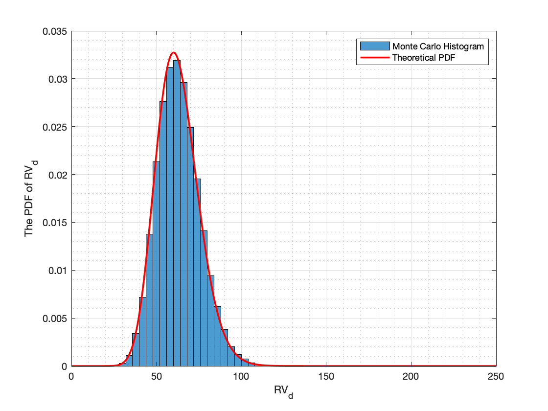
Refer to caption
a RVd:N=52,σ=0.08RV_{d}:N=52,\sigma=0.08.
Refer to caption
b RVd:N=252,σ=0.08RV_{d}:N=252,\sigma=0.08.
Refer to caption
c RVd:N=52,σ=0.1RV_{d}:N=52,\sigma=0.1.
Refer to caption
d RVd:N=252,σ=0.1RV_{d}:N=252,\sigma=0.1.
Figure 2: The PDF of RVd(t1,N,T)RV_{d}(t_{1},N,T) obtained by using the Laguerre expansion (14) whereas the corresponding histogram computed by MC simulation.

It is clearly observed that the PDFs of RVdRV_{d} obtained from the Laguerre expansions (14) are consistent with those corresponding histograms obtained from MC simulations for all N=52,252N=52,252 and σ=0.08,0.10\sigma=0.08,0.10, as shown in Figure 2a2d.

Example 3.

In this example, we investigate the absolute values of truncation errors on fair strike prices of RVd\sqrt{RV_{d}} as presented in Theorem 3. For given K+1K+1 as a number of terms in the finite summation series (32).

By setting all parameters to the same values as in Example 1, except for N=252N=252 and varying σ\sigma which are set to 0.050.05, 0.060.06, 0.070.07, 0.080.08, 0.090.09, and 0.10.1, we evaluate the accuracy and efficiency of Kvol11K^{1}_{vol_{1}}. Specifically, five sequences of truncation errors εK,(βwidebar,μwidebar0)(,ν)\varepsilon_{K,\infty}^{(\widebar{\beta},\widebar{\mu}_{0})}(\ell,\nu) are computed for three different values of the degree of mean reversion κ\kappa, i.e. κ1=0.5,κ2=1.5\kappa_{1}=0.5,\kappa_{2}=1.5, and κ3=3.0\kappa_{3}=3.0, using equation (29), as summarized in Table 1. By choosing K=3K=3, we obtain

|ε3,(βwidebar,μwidebar0)(,ν)|=|Kvol11Kvol1,31|<2.3101E08\left|\varepsilon_{3,\infty}^{(\widebar{\beta},\widebar{\mu}_{0})}(\ell,\nu)\right|=\left|K^{1}_{vol_{1}}-K^{1}_{{vol_{1}},3}\right|<2.3101\text{E}-08

for all values of σ\sigma and κ\kappa, indicating that K=3K=3 yields sufficiently accurate results. Therefore, we adopt K=3K=3 in our subsequent experiments.

κ\kappa KK σ=0.05\sigma=0.05 σ=0.06\sigma=0.06 σ=0.07\sigma=0.07 σ=0.08\sigma=0.08 σ=0.09\sigma=0.09 σ=0.10\sigma=0.10
0.5 0 5.0621E-03 4.0908E-03 3.3784E-03 2.8286E-03 2.3877E-03 2.0238E-03
1 2.4812E-06 1.3472E-06 7.8533E-07 4.7996E-07 3.0264E-07 1.9458E-07
2 2.3443E-09 8.5308E-10 3.4989E-10 1.5546E-10 7.2847E-11 3.5296E-11
3 2.6654E-12 6.4748E-13 1.8563E-13 6.0396E-14 1.9540E-14 7.1054E-15
1.5 0 2.2769E-02 1.8416E-02 1.5221E-02 1.2749E-02 1.0760E-02 9.1092E-03
1 5.0288E-05 2.7367E-05 1.5987E-05 9.7862E-06 6.1741E-06 3.9644E-06
2 2.1434E-07 7.8326E-08 3.2261E-08 1.4386E-08 6.7571E-09 3.2735E-09
3 1.1008E-09 2.6957E-10 7.8065E-11 2.5270E-11 8.7965E-12 3.1957E-12
3.0 0 4.8567E-02 3.9763E-02 3.3365E-02 2.8470E-02 2.4577E-02 2.1387E-02
1 2.2947E-04 1.2806E-04 7.7190E-05 4.9107E-05 3.2476E-05 2.2088E-05
2 2.0955E-06 7.9627E-07 3.4435E-07 1.6308E-07 8.2467E-08 4.3744E-08
3 2.3101E-08 5.9702E-09 1.8497E-09 6.5101E-10 2.5122E-10 1.0367E-10
Table 1: The values of |εK,(βwidebar,μwidebar0)(,ν)|\left|\varepsilon_{K,\infty}^{(\widebar{\beta},\widebar{\mu}_{0})}(\ell,\nu)\right|, evaluated by (4.3) with =1/2\ell=1/2 and N=252N=252, are computed based on the parameter settings in Example 3, with different values of price volatility σ\sigma and degree of the mean reversions κ\kappa.

By setting σ=0.5\sigma=0.5, we plot the convergence of MC volatility swap prices to Kvol1,31K^{1}_{{vol_{1}},3} for κi\kappa_{i}, i=1,2,3i=1,2,3. Three sequences of MC volatility swap prices, with NpN_{p} varying from 1×1031\times 10^{3} to 1×1051\times 10^{5}, are plotted against Kvol1,31K^{1}_{{vol_{1}},3} for each value of κ\kappa, as shown in Figures 3a3c, and 3e, respectively. Additionally, we plot the corresponding sequences of variances of the MC volatility swap prices for κi\kappa_{i}, i=1,2,3i=1,2,3, in Figures 3b3d, and 3f, respectively.

Refer to caption
a Volatility swap prices when κ=0.5\kappa=0.5
Refer to caption
b Variances of volatility swap price when κ=0.5\kappa=0.5
Refer to caption
c Variances of volatility swap price when κ=1.5\kappa=1.5
Refer to caption
d Variances of volatility swap price when κ=1.5\kappa=1.5
Refer to caption
e Variances of volatility swap price when κ=3.0\kappa=3.0
Refer to caption
f Variances of volatility swap price when κ=3.0\kappa=3.0
Figure 3: The convergences of the MC volatility swap prices compared with Kvol1,31K^{1}_{{vol_{1}},3} computed using (32), and the convergences the variances of the MC volatility swap prices to zero.

As shown in Figures 3a3b, the MC volatility swap prices converge to Kvol1,31K^{1}_{{vol_{1}},3}, and the variances of the MC volatility swap prices approach zero, confirming that the MC estimates are very close to the true value of Kvol1,31K^{1}_{{vol_{1}},3}. Similar convergence behavior is observed for κ2=1.5\kappa_{2}=1.5 and κ3=3\kappa_{3}=3, as illustrated in Figures 3c3d and Figures 3e3f, respectively. Moreover, as shown in Figures 3a3c, and 3e, it can be observed that increasing the value of κ\kappa results in slower convergence of the MC simulation results toward the analytical values.

7.2 Effects on fair strike prices of volatility and variance swaps

Example 4.

This example is studied on the effects of price volatility σ\sigma in Schwartz one-factor model (2) on fair strike prices of volatility and variance swaps presented in Theorems 4 and 5, respectively.

Let T=1,Δt=TN1,t1=0T=1,\Delta t=\frac{T}{N-1},t_{1}=0 and ti=(i1)Δtt_{i}=(i-1)\Delta t for i=2,,Ni=2,\ldots,N. To measure the effects of the price volatility σ\sigma on fair strike prices of volatility and variance swaps changing in the closed interval of time [t1,T][t_{1},T], we set S0=2S_{0}=2 and μ=1\mu=1. We then obtain a variation of Zi=XtiXti1=lnStilnSti1Z_{i}=X_{t_{i}}-X_{t_{i-1}}=\ln{S_{t_{i}}}-\ln{S_{t_{i-1}}} under κi\kappa_{i}, for i=1,2,3i=1,2,3 while σ\sigma is varied over the interval [0.005,0.1][0.005,0.1]. With this parameter setting, we let N=52N=52 and then we plot the volatility swap Kvol11K^{1}_{vol_{1}} obtained from (32) against those obtained from MC simulations with Np=105N_{p}=10^{5} sample paths denoted by Kvol1MCK^{MC}_{vol_{1}}. Similarly, the variance swap Kvar11K^{1}_{var_{1}}, obtained from (34), is compared with the MC simulation results Kvar1MCK^{MC}_{var_{1}} using the same number of paths.

Refer to caption
a The volatility swap prices computed by using (32) with κi,\kappa_{i}, i=1,2,3i=1,2,3 and MC simulations.
Refer to caption
b The variance swap prices computed by using (34) with κi,\kappa_{i}, i=1,2,3i=1,2,3 and MC simulations.
Figure 4: The comparison between the variance and variance swap prices computed by using our closed-form formula (34) and (32), respectively, with the difference of prices volatility (σ\sigma) and degree of means reversion (κ\kappa), and the MC simulations.

The numerical results clearly demonstrate that the closed-form pricing formulas (34) and (32) yield values that perfectly match the results from MC simulations. Moreover, Figure 4a shows that an increase in price volatility results in the fair strike prices of volatility swaps increasing for each κi\kappa_{i} all i=1,2,3i=1,2,3. For the fair strike prices of variance swaps, similar results are shown in Figure 4b.

Example 5.

In this example, we aim to examine the effects of the number of trading days NN on fair strike prices of volatility and variance swaps, as presented in Theorems 4 and 5, respectively.

To study the effects of the number of trading days NN on fair strike prices of volatility and variance swaps, all parameters are set to be the same values as used in Example 4, except that we fix κ=κ1\kappa=\kappa_{1} and consider three values of price volatility σ:σ1=0.05,σ2=0.06\sigma:\sigma_{1}=0.05,\sigma_{2}=0.06, and σ3=0.07\sigma_{3}=0.07 . The number of observations NN is varied from 22 to 252252. We compare the results by plotting Kvol11K^{1}_{vol_{1}} against Kvol1MCK^{MC}_{vol_{1}} and Kvar11K^{1}_{var_{1}} against Kvar1MCK^{MC}_{var_{1}} as shown in the following figure.

Refer to caption
a The volatility swap prices computed by using (32) with σi,\sigma_{i}, i=1,2,3,i=1,2,3, and the MC simulations.
Refer to caption
b The variance swap prices computed by using (34) with σi,\sigma_{i}, i=1,2,3,i=1,2,3, and the MC simulations.
Figure 5: The comparison between the variance and variance swap prices computed by using our closed-form formulas (34) and (32), respectively, with the difference number of trading days (NN) and prices volatility (σ\sigma), and the MC simulations.

Figure 5a illustrates that as the number of trading days increases, the fair strike prices of the volatility swap obtained from our closed-form pricing formula (32) are consistent and converge to the results obtained from MC simulations for all σi\sigma_{i} for i=1,2,3i=1,2,3. A similar convergence pattern is observed for the variance swap prices, as shown in Figure 5b, where the prices are computed by (34).

8 Conclusion

In this paper, we first derived the distribution of the realized variance of log-returns with time-varying volatility for pricing volatility swaps under discrete-time observations, assuming the underlying asset follows the Schwartz one-factor model. We demonstrated that the realized variance is in the class of generalized noncentral chi-square distributions, as introduced by Koutras [17] in 1986, and can be expressed as a linear combination of independent noncentral chi-square random variables with weighted parameters. Based on this result, we derived the first analytical pricing formulas for volatility and variance swaps, as well as for volatility and variance options, under both time-varying and constant volatility cases. To support practical implementation, we provided an error analysis and proposed simple closed-form approximations for pricing volatility derivatives under the Schwartz model. Numerical experiments were conducted, clearly demonstrating the accuracy and computational efficiency of the proposed formulas and their consistency with Monte Carlo simulations. Finally, we analyzed the effects of price volatility and the number of trading days on the fair strike prices of volatility and variance swaps. The results show that increasing price volatility leads to higher fair strike prices, while increasing the number of trading days causes the fair strike prices to converge to their true values. Overall, the newly derived analytical formulas significantly enhance computational efficiency, particularly for pricing volatility derivatives with square-root payoffs. This contributes a practical and effective tool for both researchers and practitioners in the financial derivatives market.

Acknowledgement

We would like to express our sincere gratitude to the Development and Promotion of Science and Technology Talents Project (DPST) for supporting this research. We also thank the anonymous reviewers for their valuable comments and recommendations, which have helped to improve the quality and clarity of this work. Any remaining errors are solely our own.

References

  • [1] Blanco, Carlos and Soronow, David. Mean reverting processes-energy price processes used for derivatives pricing & risk management. Commodities now , 5(2):68–72, 2001.
  • [2] Brockhaus, Oliver and Long, Douglas. Volatility swaps made simple. Risk-London-Risk Magazine Limited , 13(1):92–95, 2000.
  • [3] Castaño-Martínez, Antonia and López-Blázquez, Fernando. Distribution of a sum of weighted noncentral chi-square variables. Test, 14(2):397–415, 2005.
  • [4] Chan, Leunglung and Platen, Eckhard. Pricing volatility derivatives under the modified constant elasticity of variance model. Operations Research Letters, 43(4):419–422, 2015.
  • [5] Chumpong, Kittisak and Mekchay, Khamron and Thamrongrat, Nopporn. Analytical formulas for pricing discretely-sampled skewness and kurtosis swaps based on Schwartz’s one-factor model. Songklanakarin J. Sci. Technol, 43(2):1–6, 2021.
  • [6] Chunhawiksit, Chonnawat and Rujivan, Sanae Pricing discretely-sampled variance swaps on commodities. Thai Journal of Mathematics, 14(3):711–724, 2016.
  • [7] Davis, AW. A differential equation approach to linear combinations of independent chi-squares. Journal of the American Statistical Association, 72(357):212–214, 1977.
  • [8] Demeterfi, Kresimir, Derman, Emanuel, and Kamal, Michael. A guide to volatility and variance swaps. Journal of Derivatives, 6(4):9–32, 1999.
  • [9] Duangpan, Ampol, Boonklurb, Ratinan, Chumpong, Kittisak, and Sutthimat, Phiraphat. Analytical formulas for conditional mixed moments of generalized stochastic correlation process. Symmetry, 14(5):897, 2022.
  • [10] Dufresne, Daniel. Laguerre series for Asian and other options. Mathematical Finance, 10(4):407–428, 2000.
  • [11] García Franco, José Carlos. Maximum likelihood estimation of mean reverting processes. Technical Report, Citeseer, 2023. https://www2.stat.duke.edu/˜scs/Projects/StructuralPhylogeny/OUprocess.pdf
  • [12] Hull, John C. and Basu, Sankarshan. Options, Futures, and Other Derivatives. Pearson Education India, 2016.
  • [13] Javaheri, Alireza, Wilmott, Paul, and Haug, Espen G. GARCH and volatility swaps. Quantitative Finance, 4(5):589–595, 2004.
  • [14] Johnson, Norman L., Kotz, Samuel, and Balakrishnan, Narayanaswamy. Continuous Univariate Distributions, Volume 2. John Wiley & Sons, 1995.
  • [15] Jouini, Elyès, Cvitanić, Jakša, and Musiela, Marek. Option Pricing, Interest Rates and Risk Management. Cambridge University Press, 2001.
  • [16] Kotz, Samuel, Johnson, Norman L., and Boyd, D. W. Series representations of distributions of quadratic forms in normal variables II. Non-central case. The Annals of Mathematical Statistics, 38(3):838–848, 1967.
  • [17] Koutras, Markos. On the generalized noncentral chi-squared distribution induced by an elliptical gamma law. Biometrika, 73(2):528–532, 1986.
  • [18] Ma, JunMei and Xu, Chenglong. An efficient control variate method for pricing variance derivatives. Journal of Computational and Applied Mathematics, 235(1):108–119, 2010.
  • [19] Mehta, Nina. Equity vol swaps grow up. Derivatives Strategy Magazine, 1999.
  • [20] Mirevski, S. P. and Boyadjiev, L. On some fractional generalizations of the Laguerre polynomials and the Kummer function. Computers & Mathematics with Applications, 59(3):1271–1277, 2010.
  • [21] Olver, Frank W. J. NIST Handbook of Mathematical Functions Hardback and CD-ROM. Cambridge University Press, 2010.
  • [22] Ruben, Harold. Probability content of regions under spherical normal distributions, IV: The distribution of homogeneous and non-homogeneous quadratic functions of normal variables. The Annals of Mathematical Statistics, 33(2):542–570, 1962.
  • [23] Rujivan, Sanae and Rakwongwan, Udomsak. Analytically pricing volatility swaps and volatility options with discrete sampling: Nonlinear payoff volatility derivatives. Communications in Nonlinear Science and Numerical Simulation, 100:105849, 2021.
  • [24] Rujivan, Sanae and Zhu, Song-Ping. A simplified analytical approach for pricing discretely-sampled variance swaps with stochastic volatility. Applied Mathematics Letters, 25(11):1644–1650, 2012.
  • [25] Schwartz, Eduardo S. The stochastic behavior of commodity prices: Implications for valuation and hedging. The Journal of Finance, 52(3):923–973, 1997.
  • [26] Shah, B. K. Distribution of definite and of indefinite quadratic forms from a non-central normal distribution. The Annals of Mathematical Statistics, 34(1):186–190, 1963.
  • [27] Shah, B. K. and Khatri, C. G. Distribution of a definite quadratic form for non-central normal variates. The Annals of Mathematical Statistics, pages 883–887, 1961.
  • [28] Shen, Yang and Siu, Tak Kuen. Pricing variance swaps under a stochastic interest rate and volatility model with regime-switching. Operations Research Letters, 41(2):180–187, 2013.
  • [29] Slater, Lucy Joan. Generalized Hypergeometric Functions. Cambridge University Press, UK, 1966.
  • [30] Stuart, Alan, Ord, J. Keith, and Arnold, Steven. Kendall’s advanced theory of statistics. vol. 2a: Classical inference and the linear model. Kendall’s Advanced Theory of Statistics. Vol. 2A: Classical Inference and the Linear Model, 1999.
  • [31] Sutthimat, Phiraphat and Mekchay, Khamron. Closed-form formulas for conditional moments of inhomogeneous Pearson diffusion processes. Communications in Nonlinear Science and Numerical Simulation, 106:106095, 2022.
  • [32] Swishchuk, Anatoliy V. Variance and volatility swaps in energy markets. Available at SSRN 1628178, 2010.
  • [33] Théoret, Raymond, Zabré, Lydie, and Rostan, Pierre. Pricing volatility swaps: empirical testing with Canadian data. [Université du Québec à Montréal], Centre de recherche en gestion, 2002.
  • [34] Weraprasertsakun, Anurak and Rujivan, Sanae. A closed-form formula for pricing variance swaps on commodities. Vietnam Journal of Mathematics, 45(1-2):255–264, 2017.
  • [35] Windcliff, Heath, Forsyth, Peter A., and Vetzal, Kenneth R. Pricing methods and hedging strategies for volatility derivatives. Journal of Banking & Finance, 30(2):409–431, 2006.
  • [36] Zheng, Wendong and Kwok, Yue Kuen. Closed form pricing formulas for discretely sampled generalized variance swaps. Mathematical Finance, 24(4):855–881, 2014.
  • [37] Zhu, Song-Ping and Lian, Guang-Hua. A closed-form exact solution for pricing variance swaps with stochastic volatility. Mathematical Finance: An International Journal of Mathematics, Statistics and Financial Economics, 21(2):233–256, 2011.