Three loop master integrals for ${\mathcal{O}}(\alpha\alpha_{s}^{2})$ corrections to quark form factor

Abstract

We consider the three-loop mixed strong-electroweak (${\mathcal{O}}(\alpha\alpha_{s}^{2})$) corrections to the quark form factor. We compute the master integrals which are appearing in the Feynman diagrams containing a single massive boson in the loop. We use the state-of-the-art method of differential equations to compute all 303 of them, expressing the results in terms of generalized polylogarithms. We encounter multiple square roots that cannot be simultaneously rationalized using a single transformation. Applying concurrent transformations allows us to express the results through generalized polylogarithms with a simple alphabet, but with multiple interdependent arguments.

1 Introduction

Scattering amplitudes are essential for computing hard scattering processes in perturbative Quantum Chromodynamics (QCD). Beyond delivering precise phenomenological predictions, the scattering amplitudes provide a clear insight into the underlying principles of Quantum Field Theory such as factorization or the universality of infrared (IR) singularities. The simplest amplitudes, known as form factors, involve two on-shell states of elementary fields, either both massless (quarks or gluons) Ravindran:2004mb ; deFlorian:2013sza ; Moch:2005tm ; Moch:2005id ; Baikov:2009bg ; Gehrmann:2010ue ; Gehrmann:2014vha ; Ahmed:2015qia ; Ahmed:2015qpa ; Ahmed:2016vgl ; Ahmed:2016qjf ; Ahmed:2019yjt ; Lee:2021lkc ; Lee:2022nhh ; Chakraborty:2022yan or both massive (quarks) Bernreuther:2004ih ; Bernreuther:2004th ; Bernreuther:2005rw ; Bernreuther:2005gw ; Gluza:2009yy ; Ablinger:2017hst ; Henn:2016tyf ; Lee:2018nxa ; Ablinger:2018yae ; Lee:2018rgs ; Blumlein:2019oas ; Fael:2022rgm ; Fael:2022miw ; Fael:2023zqr ; Blumlein:2023uuq or one massless and one massive Bonciani:2008wf ; Huber:2009se ; Bell:2006tz ; Bell:2010mg ; Chen:2018dpt ; Engel:2018fsb ; Datta:2023otd ; Fael:2024vko ; Datta:2024cen , and an off-shell state described through a composite operator. One such form factor, the quark form factor, plays a significant role in precise phenomenological predictions for the Drell-Yan (DY) production of a lepton pairs. This process stands as a cornerstone for physics investigations at the Large Hadron Collider (LHC). Beyond its role in precisely determining key parameters of the weak interaction, such as the sine of the weak mixing angle and the W boson mass, the DY process is instrumental for constraining parton distribution functions (PDFs), calibrating detectors, and establishing collider luminosity. Furthermore, its final state signatures closely resemble those predicted by numerous beyond-the-Standard-Model (BSM) theories, making it a critical Standard Model (SM) background in the search for New Physics.

Given its significant relevance, the DY process has been measured experimentally with great precision and has also been computed theoretically to a high degree of accuracy. Indeed, the DY process was one of the earliest to have radiative corrections computed, considering both strong ($\alpha_{s}$) and electroweak (EW) ($\alpha$) couplings. The next-to-leading-order (NLO) Altarelli:1979ub and next-to-next-to-leading-order (NNLO) Hamberg:1990np ; Harlander:2002wh QCD corrections to the total cross section were followed by differential NNLO calculations incorporating leptonic decays Anastasiou:2003yy ; Anastasiou:2003ds ; Melnikov:2006kv ; Catani:2009sm ; Catani:2010en . Complete EW corrections have been calculated for $W$ Dittmaier:2001ay ; Baur:2004ig ; Zykunov:2006yb ; Arbuzov:2005dd ; CarloniCalame:2006zq and $Z$ Baur:2001ze ; Zykunov:2005tc ; CarloniCalame:2007cd ; Arbuzov:2007db ; Dittmaier:2009cr production. Recent advancements include next-to-next-to-next-to-leading-order (N³LO) QCD radiative calculations for both the inclusive Duhr:2020seh ; Chen:2021vtu ; Duhr:2020sdp as well as fiducial Camarda:2021ict ; Chen:2022cgv ; Neumann:2022lft ; Campbell:2023lcy production cross section, and NNLO mixed QCD-EW corrections Dittmaier:2014qza ; Dittmaier:2015rxo ; Bonciani:2016wya ; Bonciani:2019nuy ; Bonciani:2020tvf ; Buccioni:2020cfi ; Behring:2020cqi ; Buonocore:2021rxx ; Bonciani:2021zzf ; Bonciani:2021iis ; Buccioni:2022kgy ; Armadillo:2022bgm ; Dittmaier:2024row ; Armadillo:2024nwk . Notably, these mixed QCD-EW corrections have proven larger than anticipated, highlighting the necessity of including other corrections such as N³LO mixed QCD-EW (${\mathcal{O}}(\alpha\alpha_{s}^{2})$) corrections. Quark form factors at ${\mathcal{O}}(\alpha\alpha_{s}^{2})$ are a key component in obtaining these higher-order corrections.

The state-of-the-art approach to computing these virtual amplitudes involves reducing scalar Feynman integrals to a linearly independent basis, known as Master Integrals (MIs), through integration-by-parts (IBP) Tkachov:1981wb ; Chetyrkin:1981qh ; Laporta:2001dd and Lorentz invariance (LI) identities. Subsequently, the MIs are computed using the method of differential equations Kotikov:1990kg ; Remiddi:1997ny ; Gehrmann:1999as ; Argeri:2007up ; Henn:2013pwa ; Henn:2014qga ; Ablinger:2015tua ; Ablinger:2018zwz . The basic principle of this technique involves differentiating the MIs with respect to the kinematic variables and then applying IBP identities to the resulting expressions. This process yields a system of first-order coupled differential equations. By strategically organizing this system into a block-triangular form, a solution can be obtained either through a bottom-up or top-down approach. The sub-systems can be decoupled to form higher-order differential equations, which are subsequently solved using the method of variation of constants. This powerful technique can even be improved Henn:2013pwa ; Henn:2014qga if the system can be reduced to canonical form or $\epsilon$-form where each MIs can be solved in terms of iterated integrals such as harmonic polylogarithms (HPLs) Remiddi:1999ew , generalized harmonic polylogarithms (GPLs) Goncharov:2001iea ; Vollinga:2004sn , Chen iterated integrals Chen:1977oja etc. In this paper, we present the computation of MIs relevant to the ${\mathcal{O}}(\alpha\alpha_{s}^{2})$ corrections to quark form factors at three loops. We categorize the contributing Feynman diagram topologies into three groups based on the EW bosons involved. First, diagrams with a photon in the loop, photon being massless, exhibit topologies that are subsets of those found in three-loop QCD corrections. Second, diagrams featuring a triple vector boson vertex have topologies that are again subsets, this time of those appearing in three-loop mixed QCD-EW corrections to Higgs boson production, as presented in Bonetti:2017ovy . Third, we consider Feynman diagrams containing a single $Z$ or $W$ boson. The MIs appearing in these topologies are novel and are the focus of this paper.

The remainder of this paper is organized as follows. Section 2 establishes our notation and details the choice of the Feynman prescription for all introduced variables. In Section 3, we detail the computational approach, specifying the integral families, presenting our choice of MIs, and commenting on their analytic evaluation using the method of differential equations. The findings of this work are presented in Section 4, and Section 5 provides the concluding remarks.

2 Notation

In this section, we establish our notation. We define the physical scattering process, and introduce the required dimensionless variables. We consider the scattering process of an off-shell vector boson ($Z$) production with virtuality $q^{2}$, in quark-antiquark annihilation

$$q(p_{1})+\bar{q}(p_{2})\rightarrow Z(q)\,,$$ (1)

where the incoming quark and anti-quark carry $p_{1}$ and $p_{2}$ momenta, respectively, with the on-shell conditions

$$p_{1}^{2}=0\,,~~p_{2}^{2}=0\,.$$ (2)

We also introduce the following dimensionless variables

$$-\frac{q^{2}}{m_{V}^{2}}=-\frac{s}{m_{V}^{2}}=x=\frac{(1+x_{l})^{2}}{x_{l}}=\frac{x_{n}}{(1+x_{n})^{2}}=-x_{i}^{2}\,,$$ (3)

where $m_{V}$ denotes the mass of the vector boson ($Z$ or $W$) present in the loop. We consider the three-loop mixed QCD-EW corrections (${\mathcal{O}}(\alpha\alpha_{s}^{2})$) to this reaction. As mentioned earlier, we focus on the MIs linked to topologies in Feynman diagrams that include a massive vector boson propagator in the loop.

We have introduced three parameters $x_{l}$, $x_{n}$ and $x_{i}$ as suitable base transformations to rationalize the roots that appear while solving the differential equations. Therefore, the final expressions for our results involve GPLs with arguments $x,x_{l},x_{n}$ and $x_{i}$, as well as polynomials of these variables. The variable $x$ is defined such that, in the unphysical region ($s<0$), x is real and positive. To perform the analytic continuation to the physical region, the Feynman prescription on the invariants is required. In the physical region, $s$ is positive with a positive infinitesimal imaginary part, $s+i0^{+}$. Hence, $x$ is given by

$$x\rightarrow x-i0^{+}\,.$$ (4)

In terms of $s$, $x_{l}$ can be solved to obtain the following two roots

$$x_{l}^{(\pm)}=\frac{\sqrt{s+i0^{+}}\mp\sqrt{4m_{V}^{2}+s+i0^{+}}}{\sqrt{s+i0^{+}}\pm\sqrt{4m_{V}^{2}+s+i0^{+}}}\,.$$ (5)

1. For $s\geq 0$, both $x_{l}^{(\pm)}$ are negative-valued real numbers, with modulus less than or greater than one, respectively. The prescription becomes $x_{l}^{(\pm)}=-w_{\pm}\mp i0^{+}$, where $w_{\pm}$ are the absolute values of the roots.

2. For $-4m_{V}^{2}<s<0$, both $x_{l}^{(\pm)}$ are complex numbers that lie on the upper and lower half of the unit circle, respectively.

3. For $s\leq-4m_{V}^{2}$, both $x_{l}^{(\pm)}$ are positive-valued real numbers, with modulus less than and greater than one, respectively.

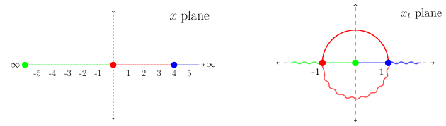
Figure 1: The figure illustrates the variable transformation between $x$ and $x_{l}$. The left and right panel displays the $x$-plane and the complex $x_{l}$-plane, respectively. Colored lines show the mapping of intervals. In the $x_{l}$-plane, straight and wiggly lines represent two distinct roots.

In Fig.1, we illustrate the transformation $x\rightarrow x_{l}$. We choose the root $x_{l}^{(+)}$ which maps the real axis of the complex $x$-plane into the unit circle (solid lines) in the $x_{l}$-plane. The kinematic points $x\rightarrow 0,x\rightarrow 4$ and $x\rightarrow\pm\infty$ in the $x$-plane correspond to $x_{l}\rightarrow-1$ (red dot), $x_{l}\rightarrow 1$ (blue dot) and $x_{l}\rightarrow 0^{\pm}$ (green dot), respectively. The intervals $x<0$, $0<x<4$ and $x>4$ are mapped to $-1<x_{l}<0$, the upper semi-circle, and $0<x_{l}<1$, respectively. Due to our chosen Feynman prescription ($s+i0^{+}$), the green and blue lines in the $x_{l}$ plane lie infinitesimally above and below the real axis, respectively.

Similarly, $x_{n}$ can be solved to obtain the following two roots.

$$x_{n}(\pm)=\frac{m_{V}\mp\sqrt{m_{V}^{2}+4s+i0^{+}}}{m_{V}\pm\sqrt{m_{V}^{2}+4s+i0^{+}}}\,.$$ (6)

1. For $s>0$, both roots $x_{n}^{(\pm)}$ are negative-valued real numbers, with modulus less than or greater than one, respectively. Our choice of the Feynman prescription gives $x_{n}^{(\pm)}=-{w_{n}}_{\pm}\pm i0^{+}$, where $w_{n}$ are the moduli of the roots.

2. For $-\frac{m_{V}^{2}}{4}<s<0$, the roots $x_{n}^{(\pm)}$ are positive-valued real numbers, with modulus less than or greater than one, respectively.

3. For $s\leq-\frac{m_{V}^{2}}{4}$, the roots $x_{n}^{(\pm)}$ are complex numbers that lie on the lower and upper half of the unit circle, respectively.

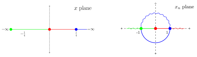
Figure 2: Same as Fig. 1, but for the variable transformation between $x$ and $x_{n}$.

In Fig.2, we illustrate the transformation $x\rightarrow x_{n}$. We choose the root $x_{n}^{(+)}$ which maps the real axis of the complex $x$-plane into the unit circle (solid lines) in the $x_{n}$-plane.

$x_{i}$ can be trivially solved in terms of $s$ as

$$x_{i}^{(\pm)}=\mp\sqrt{\frac{s+i0^{+}}{m_{V}^{2}}}\,.$$ (7)

In the physical region, both roots are real. Conversely, Feynman integrals are complex, so expressing them using GPLs in terms of $x_{i}$ introduces an explicit $i\pi$ term. The sign of this term inherently depends on the prescription chosen. To present prescription-independent results, we explicitly isolate the logarithms from all GPLs and consistently express logarithms of $x_{i}$ to $\log(x)$.

3 Computational details

We adopt the conventional approach for obtaining and computing the MIs. Initially, we have identified the integral families and their corresponding sectors that fully encompass the relevant Feynman diagrams which appear in the physical process. The identification has been performed using Reduze vonManteuffel:2012np . We have then carried out the IBP reduction with the help of Kira Maierhofer:2017gsa ; Klappert:2020nbg , which yielded a total of 303 MIs. Subsequently, we have utilized the method of differential equations to solve these MIs. The specifics of each step are detailed in this section.

3.1 Integral families

Each integral family contains three auxiliary propagators. Thus, a strategic selection would result in a minimal set of integral families. However, for convenience in the IBP reduction process, we deliberately choose the following 25 integral families. We begin by defining the notation to represent the inverse of the propagator within these integral families as follows.

$${\cal P}_{i}=k_{i}^{2}\,,~~~{\cal P}_{ij}=(k_{i}-k_{j})^{2}\,,~~~{\cal P}_{123}=(k_{1}+k_{2}-k_{3})^{2}\,,~~~{\cal P}_{i;j}=(k_{i}-p_{j})^{2}\,,~~$$

$${\cal P}_{i;12}=(k_{i}-p_{1}-p_{2})^{2}\,,~~{\cal P}_{23;1}=(k_{2}-k_{3}-p_{1})^{2}\,,~~{\cal P}_{23;-2}=(k_{2}-k_{3}+p_{2})^{2}\,.$$ (8)

In the preceding definitions, the indices $i$ and $j$ take the values 1, 2, and 3. Now we present the 25 integral families.

$${\cal I}_{1}:\{{\cal P}_{1},{\cal P}_{2},{\cal P}_{3},{\cal P}_{12}-m_{V}^{2},{\cal P}_{23},{\cal P}_{13},{\cal P}_{1;1},{\cal P}_{2;1},{\cal P}_{3;1},{\cal P}_{1;12},{\cal P}_{2;12},{\cal P}_{3;12}\}$$

$${\cal I}_{2}:\{{\cal P}_{1},{\cal P}_{2},{\cal P}_{3},{\cal P}_{12},{\cal P}_{23},{\cal P}_{13},{\cal P}_{1;1}-m_{V}^{2},{\cal P}_{2;1},{\cal P}_{3;1},{\cal P}_{1;12},{\cal P}_{2;12},{\cal P}_{3;12}\}$$

$${\cal I}_{3}:\{{\cal P}_{1}-m_{V}^{2},{\cal P}_{2},{\cal P}_{3},{\cal P}_{12},{\cal P}_{23},{\cal P}_{13},{\cal P}_{1;1},{\cal P}_{2;1},{\cal P}_{3;1},{\cal P}_{1;12},{\cal P}_{2;12},{\cal P}_{3;12}\}$$

$${\cal I}_{4}:\{{\cal P}_{1},{\cal P}_{2},{\cal P}_{3},{\cal P}_{12},{\cal P}_{23},{\cal P}_{13},{\cal P}_{1;1},{\cal P}_{2;1},{\cal P}_{3;1},{\cal P}_{1;12}-m_{V}^{2},{\cal P}_{2;12},{\cal P}_{3;12}\}$$

$${\cal I}_{5}:\{{\cal P}_{1},{\cal P}_{2},{\cal P}_{3},{\cal P}_{12}-m_{V}^{2},{\cal P}_{23},{\cal P}_{13},{\cal P}_{1;1},{\cal P}_{2;1},{\cal P}_{23;1},{\cal P}_{1;12},{\cal P}_{2;12},{\cal P}_{3;12}\}$$

$${\cal I}_{6}:\{{\cal P}_{1},{\cal P}_{2},{\cal P}_{3},{\cal P}_{12}-m_{V}^{2},{\cal P}_{23},{\cal P}_{13},{\cal P}_{1;1},{\cal P}_{2;1},{\cal P}_{23;-2},{\cal P}_{1;12},{\cal P}_{2;12},{\cal P}_{3;12}\}$$

$${\cal I}_{7}:\{{\cal P}_{1},{\cal P}_{2},{\cal P}_{3},{\cal P}_{12},{\cal P}_{23},{\cal P}_{13},{\cal P}_{1;1},{\cal P}_{2;1},{\cal P}_{23;1}-m_{V}^{2},{\cal P}_{1;12},{\cal P}_{2;12},{\cal P}_{3;12}\}$$

$${\cal I}_{8}:\{{\cal P}_{1},{\cal P}_{2},{\cal P}_{3},{\cal P}_{12},{\cal P}_{23},{\cal P}_{13},{\cal P}_{1;1},{\cal P}_{2;1},{\cal P}_{23;-2}-m_{V}^{2},{\cal P}_{1;12},{\cal P}_{2;12},{\cal P}_{3;12}\}$$

$${\cal I}_{9}:\{{\cal P}_{1},{\cal P}_{2},{\cal P}_{3},{\cal P}_{12},{\cal P}_{23},{\cal P}_{13}-m_{V}^{2},{\cal P}_{1;1},{\cal P}_{2;1},{\cal P}_{23;1},{\cal P}_{1;12},{\cal P}_{2;12},{\cal P}_{3;12}\}$$

$${\cal I}_{10}:\{{\cal P}_{1},{\cal P}_{2},{\cal P}_{3},{\cal P}_{12},{\cal P}_{23},{\cal P}_{13}-m_{V}^{2},{\cal P}_{1;1},{\cal P}_{2;1},{\cal P}_{23;-2},{\cal P}_{1;12},{\cal P}_{2;12},{\cal P}_{3;12}\}$$

$${\cal I}_{11}:\{{\cal P}_{1},{\cal P}_{2},{\cal P}_{3},{\cal P}_{12},{\cal P}_{23},{\cal P}_{13},{\cal P}_{1;1},{\cal P}_{2;1}-m_{V}^{2},{\cal P}_{23;1},{\cal P}_{1;12},{\cal P}_{2;12},{\cal P}_{3;12}\}$$

$${\cal I}_{12}:\{{\cal P}_{1},{\cal P}_{2},{\cal P}_{3},{\cal P}_{12},{\cal P}_{23},{\cal P}_{13},{\cal P}_{1;1},{\cal P}_{2;1}-m_{V}^{2},{\cal P}_{23;-2},{\cal P}_{1;12},{\cal P}_{2;12},{\cal P}_{3;12}\}$$

$${\cal I}_{13}:\{{\cal P}_{1},{\cal P}_{2},{\cal P}_{3},{\cal P}_{12},{\cal P}_{23},{\cal P}_{13},{\cal P}_{1;1},{\cal P}_{2;1},{\cal P}_{23;1},{\cal P}_{1;12},{\cal P}_{2;12},{\cal P}_{3;12}-m_{V}^{2},$$

$${\cal I}_{14}:\{{\cal P}_{1},{\cal P}_{2},{\cal P}_{3},{\cal P}_{12},{\cal P}_{23},{\cal P}_{13},{\cal P}_{1;1},{\cal P}_{2;1},{\cal P}_{23;-2},{\cal P}_{1;12},{\cal P}_{2;12},{\cal P}_{3;12}-m_{V}^{2},$$

$${\cal I}_{15}:\{{\cal P}_{1},{\cal P}_{2},{\cal P}_{3}-m_{V}^{2},{\cal P}_{12},{\cal P}_{23},{\cal P}_{13},{\cal P}_{1;1},{\cal P}_{2;1},{\cal P}_{23;1},{\cal P}_{1;12},{\cal P}_{2;12},{\cal P}_{3;12}\}$$

$${\cal I}_{16}:\{{\cal P}_{1},{\cal P}_{2},{\cal P}_{3},{\cal P}_{12},{\cal P}_{23},{\cal P}_{13},{\cal P}_{1;1}-m_{V}^{2},{\cal P}_{2;1},{\cal P}_{23;1},{\cal P}_{1;12},{\cal P}_{2;12},{\cal P}_{3;12}\}$$

$${\cal I}_{17}:\{{\cal P}_{1},{\cal P}_{2},{\cal P}_{3},{\cal P}_{12},{\cal P}_{23},{\cal P}_{13},{\cal P}_{1;1}-m_{V}^{2},{\cal P}_{2;1},{\cal P}_{23;-2},{\cal P}_{1;12},{\cal P}_{2;12},{\cal P}_{3;12}\}$$

$${\cal I}_{18}:\{{\cal P}_{1},{\cal P}_{2},{\cal P}_{3},{\cal P}_{12},{\cal P}_{23}-m_{V}^{2},{\cal P}_{13},{\cal P}_{1;1},{\cal P}_{2;1},{\cal P}_{23;1},{\cal P}_{1;12},{\cal P}_{2;12},{\cal P}_{3;12}\}$$

$${\cal I}_{19}:\{{\cal P}_{1},{\cal P}_{2},{\cal P}_{3},{\cal P}_{12},{\cal P}_{23}-m_{V}^{2},{\cal P}_{13},{\cal P}_{1;1},{\cal P}_{2;1},{\cal P}_{23;-2},{\cal P}_{1;12},{\cal P}_{2;12},{\cal P}_{3;12}\}$$

$${\cal I}_{20}:\{{\cal P}_{1},{\cal P}_{2}-m_{V}^{2},{\cal P}_{3},{\cal P}_{12},{\cal P}_{23},{\cal P}_{13},{\cal P}_{1;1},{\cal P}_{2;1},{\cal P}_{23;-2},{\cal P}_{1;12},{\cal P}_{2;12},{\cal P}_{3;12}\}$$

$${\cal I}_{21}:\{{\cal P}_{1},{\cal P}_{2},{\cal P}_{3},{\cal P}_{123},{\cal P}_{23},{\cal P}_{13},{\cal P}_{1;1},{\cal P}_{2;1},{\cal P}_{3;1},{\cal P}_{1;12}-m_{V}^{2},{\cal P}_{2;12},{\cal P}_{3;12}\}$$

$${\cal I}_{22}:\{{\cal P}_{1}-m_{V}^{2},{\cal P}_{2},{\cal P}_{3},{\cal P}_{123},{\cal P}_{23},{\cal P}_{13},{\cal P}_{1;1},{\cal P}_{2;1},{\cal P}_{3;1},{\cal P}_{1;12},{\cal P}_{2;12},{\cal P}_{3;12}\}$$

$${\cal I}_{23}:\{{\cal P}_{1},{\cal P}_{2},{\cal P}_{3},{\cal P}_{123},{\cal P}_{23},{\cal P}_{13},{\cal P}_{1;1}-m_{V}^{2},{\cal P}_{2;1},{\cal P}_{3;1},{\cal P}_{1;12},{\cal P}_{2;12},{\cal P}_{3;12}\}$$

$${\cal I}_{24}:\{{\cal P}_{1},{\cal P}_{2},{\cal P}_{3},{\cal P}_{123},{\cal P}_{23},{\cal P}_{13},{\cal P}_{1;1},{\cal P}_{2;1},{\cal P}_{3;1},{\cal P}_{1;12},{\cal P}_{2;12},{\cal P}_{3;12}-m_{V}^{2}\}$$

$${\cal I}_{25}:\{{\cal P}_{1},{\cal P}_{2},{\cal P}_{3},{\cal P}_{123}-m_{V}^{2},{\cal P}_{23},{\cal P}_{13},{\cal P}_{1;1},{\cal P}_{2;1},{\cal P}_{3;1},{\cal P}_{1;12},{\cal P}_{2;12},{\cal P}_{3;12}\}$$

We observe that certain integral families have sectors with high values. Therefore, to facilitate a smooth reduction using Kira, we have to optimize the ordering of the propagators.

3.2 Master integrals

Using Kira, we have performed the IBP reduction of the integral families mentioned above, which yielded a set of 303 MIs. We also have used LiteRed Lee:2012cn ; Lee:2013mka to improve the reduction. We now present the full list of MIs obtained in this work. To establish our notation, we first introduce the general form of a three-loop integral:

$${\cal I}_{n}(\nu_{1},\nu_{2},...,\nu_{12})(d,x)=\int\prod_{i=1}^{3}\frac{d^{d}k_{i}}{(2\pi)^{d}}\prod_{j=1}^{12}\frac{1}{D_{j}^{\nu_{j}}}\,,$$ (9)

where $D_{j}$ is the $j^{th}$ element of the list given for ${\cal I}_{n}$. We put $S_{\epsilon}=\exp(-\epsilon(\gamma_{E}-\ln(4\pi)))$ equal to one for each loop order. The MIs associated with the integral family ${\cal I}_{1}$ are as follows

$${\cal I}_{1,1} ={\cal I}_{1}(1,1,0,1,1,1,0,0,0,0,0,0).\qquad {\cal I}_{1,2}={\cal I}_{1}(0,1,1,1,0,1,0,0,0,1,0,0).$$

$${\cal I}_{1,3} ={\cal I}_{1}(0,1,1,1,0,1,0,0,0,2,0,0).\qquad {\cal I}_{1,4}={\cal I}_{1}(1,0,0,1,1,1,0,0,0,1,0,0).$$

$${\cal I}_{1,5} ={\cal I}_{1}(0,1,0,1,1,1,0,0,0,1,0,0).\qquad {\cal I}_{1,6}={\cal I}_{1}(0,1,0,1,1,1,0,0,0,2,0,0).$$

$${\cal I}_{1,7} ={\cal I}_{1}(0,0,1,1,1,0,1,0,0,0,1,0).\qquad {\cal I}_{1,8}={\cal I}_{1}(0,0,1,1,1,0,1,0,0,0,2,0).$$

$${\cal I}_{1,9} ={\cal I}_{1}(0,1,0,0,1,1,1,0,0,0,1,0).\qquad {\cal I}_{1,10}={\cal I}_{1}(0,0,1,0,1,1,1,0,0,0,1,0).$$

$${\cal I}_{1,11} ={\cal I}_{1}(1,0,1,0,1,0,0,0,0,1,1,0).\qquad {\cal I}_{1,12}={\cal I}_{1}(0,1,0,1,1,1,1,0,0,0,1,0).$$

$${\cal I}_{1,13} ={\cal I}_{1}(0,1,0,1,1,1,1,0,0,0,2,0).\qquad {\cal I}_{1,14}={\cal I}_{1}(1,1,0,0,1,1,0,0,0,1,1,0).$$

$${\cal I}_{1,15} ={\cal I}_{1}(0,0,1,0,1,1,0,0,0,1,1,0).\qquad {\cal I}_{1,16}={\cal I}_{1}(1,1,0,1,1,1,0,0,0,1,1,0).$$

$${\cal I}_{1,17} ={\cal I}_{1}(1,0,1,1,0,0,0,0,0,1,0,1).\qquad {\cal I}_{1,18}={\cal I}_{1}(1,0,1,1,1,1,0,0,0,1,1,0).$$

$${\cal I}_{1,19} ={\cal I}_{1}(0,1,1,1,0,1,1,0,0,1,1,0).\qquad {\cal I}_{1,20}={\cal I}_{1}(1,1,1,0,0,0,0,0,0,1,1,1).$$

$${\cal I}_{1,21} ={\cal I}_{1}(1,1,1,1,0,0,0,0,0,1,1,1).\qquad {\cal I}_{1,22}={\cal I}_{1}(1,1,1,1,0,0,1,0,0,0,1,1).$$

$${\cal I}_{1,23} ={\cal I}_{1}(1,0,1,1,1,0,1,0,0,0,1,0).\qquad {\cal I}_{1,24}={\cal I}_{1}(0,0,1,1,0,1,1,0,0,0,0,1).$$

$${\cal I}_{1,25} ={\cal I}_{1}(0,1,1,0,0,1,1,0,0,0,1,1).\qquad {\cal I}_{1,26}={\cal I}_{1}(0,1,1,0,1,1,1,0,0,1,1,0).$$

$${\cal I}_{1,27} ={\cal I}_{1}(1,1,0,1,1,1,1,0,0,0,1,0).\qquad {\cal I}_{1,28}={\cal I}_{1}(1,0,1,1,1,0,0,0,0,1,0,0).$$

$${\cal I}_{1,29} ={\cal I}_{1}(0,0,1,1,1,1,1,0,0,0,1,0).\qquad {\cal I}_{1,30}={\cal I}_{1}(0,0,1,1,1,1,1,0,0,0,2,0).$$

$${\cal I}_{1,31} ={\cal I}_{1}(0,0,1,1,1,1,2,0,0,0,1,0).\qquad {\cal I}_{1,32}={\cal I}_{1}(0,0,1,1,1,2,1,0,0,0,1,0).$$

$${\cal I}_{1,33} ={\cal I}_{1}(0,0,1,1,2,1,1,0,0,0,1,0).\qquad {\cal I}_{1,34}={\cal I}_{1}(0,1,1,1,1,1,1,0,0,0,1,0).$$

$${\cal I}_{1,35} ={\cal I}_{1}(0,1,1,1,1,1,2,0,0,0,1,0).\qquad {\cal I}_{1,36}={\cal I}_{1}(0,0,1,1,1,1,0,0,0,1,1,0).$$

$${\cal I}_{1,37} ={\cal I}_{1}(0,0,1,1,1,1,0,0,0,1,2,0).\qquad {\cal I}_{1,38}={\cal I}_{1}(0,0,1,1,1,1,1,0,0,1,1,0).$$

$${\cal I}_{1,39} ={\cal I}_{1}(0,0,1,1,1,1,1,0,0,2,1,0).\qquad {\cal I}_{1,40}={\cal I}_{1}(1,1,1,1,1,0,0,0,0,1,0,1).$$

$${\cal I}_{1,41} ={\cal I}_{1}(0,1,1,1,1,0,1,0,0,1,0,1).\qquad {\cal I}_{1,42}={\cal I}_{1}(1,0,1,1,1,0,0,0,0,1,1,0).$$

$${\cal I}_{1,43} ={\cal I}_{1}(0,1,1,1,0,0,1,0,0,0,1,1).\qquad {\cal I}_{1,44}={\cal I}_{1}(0,1,1,1,0,0,1,0,0,0,2,1).$$

$${\cal I}_{1,45} ={\cal I}_{1}(1,0,1,1,1,0,0,0,0,1,0,1).\qquad {\cal I}_{1,46}={\cal I}_{1}(1,0,1,1,1,0,0,0,0,1,0,2).$$

$${\cal I}_{1,47} ={\cal I}_{1}(0,0,1,1,1,0,1,0,0,0,0,1).\qquad {\cal I}_{1,48}={\cal I}_{1}(0,0,1,1,1,0,1,0,0,0,0,2).$$

$${\cal I}_{1,49} ={\cal I}_{1}(0,0,1,1,1,0,2,0,0,0,0,1).\qquad {\cal I}_{1,50}={\cal I}_{1}(1,0,1,1,1,0,1,0,0,0,0,1).$$

$${\cal I}_{1,51} ={\cal I}_{1}(0,1,1,1,1,0,1,0,0,0,0,1).\qquad {\cal I}_{1,52}={\cal I}_{1}(1,1,1,1,1,0,1,0,0,0,0,1).$$

$${\cal I}_{1,53} ={\cal I}_{1}(0,0,1,1,0,1,0,0,0,1,0,0).\qquad {\cal I}_{1,54}={\cal I}_{1}(0,0,1,1,1,0,0,0,0,1,0,0).$$

$${\cal I}_{1,55} ={\cal I}_{1}(0,0,1,1,1,0,0,0,0,2,0,0).\qquad {\cal I}_{1,56}={\cal I}_{1}(0,1,1,1,0,1,1,0,0,0,1,0).$$

$${\cal I}_{1,57} ={\cal I}_{1}(0,1,1,1,0,1,1,0,0,0,2,0).\qquad {\cal I}_{1,58}={\cal I}_{1}(0,1,0,0,1,1,0,0,0,1,0,0).$$

$${\cal I}_{1,59} ={\cal I}_{1}(0,1,1,1,0,1,1,0,0,0,0,1).\qquad {\cal I}_{1,60}={\cal I}_{1}(0,1,1,1,0,1,1,0,0,0,0,2).$$

$${\cal I}_{1,61} ={\cal I}_{1}(0,1,1,1,0,1,2,0,0,0,0,1).\qquad {\cal I}_{1,62}={\cal I}_{1}(1,0,1,1,1,0,0,0,0,0,0,0).$$

$${\cal I}_{1,63} ={\cal I}_{1}(0,1,1,1,0,0,0,0,0,1,0,1).\qquad {\cal I}_{1,64}={\cal I}_{1}(0,1,1,1,0,0,0,0,0,2,0,1).$$

$${\cal I}_{1,65} ={\cal I}_{1}(0,1,1,1,0,1,0,0,1,1,0,0).\qquad {\cal I}_{1,66}={\cal I}_{1}(0,1,1,1,0,1,0,0,1,1,1,0).$$

$${\cal I}_{1,67} ={\cal I}_{1}(0,1,1,1,0,1,0,0,1,1,2,0).\qquad {\cal I}_{1,68}={\cal I}_{1}(1,1,0,1,0,1,0,0,1,0,1,0).$$

$${\cal I}_{1,69} ={\cal I}_{1}(1,1,0,1,0,1,0,0,1,1,1,0).\qquad {\cal I}_{1,70}={\cal I}_{1}(0,1,0,1,0,1,0,0,1,1,0,0).$$

$${\cal I}_{1,71} ={\cal I}_{1}(0,1,0,1,0,1,0,0,1,2,0,0).\qquad {\cal I}_{1,72}={\cal I}_{1}(1,1,0,1,1,1,0,0,1,1,0,0).$$

$${\cal I}_{1,73} ={\cal I}_{1}(1,1,0,1,1,1,0,0,1,2,0,0).\qquad {\cal I}_{1,74}={\cal I}_{1}(1,1,0,1,1,1,0,0,2,1,0,0).$$

$${\cal I}_{1,75} ={\cal I}_{1}(1,1,0,0,1,1,0,0,1,1,0,0).\qquad {\cal I}_{1,76}={\cal I}_{1}(0,1,0,1,1,1,0,0,1,1,0,0).$$

$${\cal I}_{1,77} ={\cal I}_{1}(0,1,0,1,1,1,0,0,1,2,0,0).\qquad {\cal I}_{1,78}={\cal I}_{1}(0,1,0,1,1,1,0,0,2,1,0,0).$$

$${\cal I}_{1,79} ={\cal I}_{1}(0,1,0,1,1,2,0,0,1,1,0,0).\qquad {\cal I}_{1,80}={\cal I}_{1}(0,1,0,1,1,0,1,0,1,0,1,0).$$

$${\cal I}_{1,81} ={\cal I}_{1}(0,1,0,1,1,0,1,0,1,0,2,0).\qquad {\cal I}_{1,82}={\cal I}_{1}(0,0,1,1,1,0,1,0,1,0,1,0).$$

$${\cal I}_{1,83} ={\cal I}_{1}(0,1,1,1,1,1,1,0,1,1,1,0).\qquad {\cal I}_{1,84}={\cal I}_{1}(0,1,1,1,1,1,1,0,1,1,2,0).$$

$${\cal I}_{1,85} ={\cal I}_{1}(0,1,1,1,1,1,1,0,2,1,1,0).\qquad {\cal I}_{1,86}={\cal I}_{1}(1,0,1,1,1,0,1,1,0,0,0,1).$$

$${\cal I}_{1,87} ={\cal I}_{1}(0,0,1,0,1,1,1,1,0,0,0,1).\qquad {\cal I}_{1,88}={\cal I}_{1}(0,0,1,1,1,1,1,1,0,0,0,1).$$

$${\cal I}_{1,89} ={\cal I}_{1}(0,0,1,1,1,1,1,1,0,0,0,2).\qquad {\cal I}_{1,90}={\cal I}_{1}(0,0,1,1,1,1,1,1,0,1,0,0).$$

$${\cal I}_{1,91} ={\cal I}_{1}(1,0,1,1,1,1,0,1,0,0,0,1).\qquad {\cal I}_{1,92}={\cal I}_{1}(0,1,0,1,1,1,1,1,0,1,0,0).$$

$${\cal I}_{1,93} ={\cal I}_{1}(0,1,1,1,0,0,1,1,0,1,0,1).\qquad {\cal I}_{1,94}={\cal I}_{1}(0,1,1,1,1,1,1,1,0,1,0,1).$$

$${\cal I}_{1,95} ={\cal I}_{1}(0,1,1,1,1,1,1,1,0,1,0,2).\qquad {\cal I}_{1,96}={\cal I}_{1}(0,1,1,1,1,1,0,0,0,1,0,1).$$

The MIs belonging to the integral family ${\cal I}_{2}$ are:

$${\cal I}_{2,1} ={\cal I}_{2}(1,0,0,0,1,1,1,1,0,1,0,0).\qquad {\cal I}_{2,2}={\cal I}_{2}(1,0,0,0,1,1,1,1,0,0,1,0).$$

$${\cal I}_{2,3} ={\cal I}_{2}(1,0,0,1,0,1,1,1,0,0,0,1).\qquad {\cal I}_{2,4}={\cal I}_{2}(1,0,0,0,1,1,1,1,0,0,0,1).$$

$${\cal I}_{2,5} ={\cal I}_{2}(1,0,0,0,1,1,1,1,0,0,0,2).\qquad {\cal I}_{2,6}={\cal I}_{2}(1,0,0,1,0,1,1,0,0,0,1,1).$$

$${\cal I}_{2,7} ={\cal I}_{2}(1,0,0,1,0,1,1,1,0,0,1,1).\qquad {\cal I}_{2,8}={\cal I}_{2}(1,0,0,1,1,0,1,1,0,1,0,1).$$

$${\cal I}_{2,9} ={\cal I}_{2}(1,0,1,1,1,0,1,0,0,0,1,0).\qquad {\cal I}_{2,10}={\cal I}_{2}(1,0,2,1,1,0,1,0,0,0,1,0).$$

$${\cal I}_{2,11} ={\cal I}_{2}(1,0,1,1,1,0,1,0,0,1,0,1).\qquad {\cal I}_{2,12}={\cal I}_{2}(1,0,1,1,0,0,1,1,0,1,0,1).$$

$${\cal I}_{2,13} ={\cal I}_{2}(1,0,1,1,0,0,1,0,0,0,1,1).\qquad {\cal I}_{2,14}={\cal I}_{2}(0,0,1,1,0,1,1,0,0,0,1,1).$$

$${\cal I}_{2,15} ={\cal I}_{2}(0,0,2,1,0,1,1,0,0,0,1,1).\qquad {\cal I}_{2,16}={\cal I}_{2}(1,0,1,1,1,0,1,0,0,0,1,1).$$

$${\cal I}_{2,17} ={\cal I}_{2}(1,0,1,1,1,0,1,0,0,0,1,2).\qquad {\cal I}_{2,18}={\cal I}_{2}(1,0,1,1,0,1,1,0,0,0,1,1).$$

$${\cal I}_{2,19} ={\cal I}_{2}(1,0,1,1,0,0,1,1,0,0,1,1).\qquad {\cal I}_{2,20}={\cal I}_{2}(1,0,1,0,1,0,1,0,0,1,1,0).$$

$${\cal I}_{2,21} ={\cal I}_{2}(0,0,1,1,0,1,1,1,0,0,1,1).\qquad {\cal I}_{2,22}={\cal I}_{2}(0,0,2,1,0,1,1,1,0,0,1,1).$$

$${\cal I}_{2,23} ={\cal I}_{2}(1,0,1,1,1,0,1,1,0,0,0,1).\qquad {\cal I}_{2,24}={\cal I}_{2}(1,0,2,1,1,0,1,1,0,0,0,1).$$

$${\cal I}_{2,25} ={\cal I}_{2}(1,0,1,1,1,0,1,1,0,0,0,2).\qquad {\cal I}_{2,26}={\cal I}_{2}(1,0,1,1,0,1,1,1,0,0,0,1).$$

$${\cal I}_{2,27} ={\cal I}_{2}(1,0,1,1,1,1,1,1,0,0,1,1).\qquad {\cal I}_{2,28}={\cal I}_{2}(1,0,2,1,1,1,1,1,0,0,1,1).$$

$${\cal I}_{2,29} ={\cal I}_{2}(1,0,1,1,1,1,1,1,0,0,1,2).\qquad {\cal I}_{2,30}={\cal I}_{2}(0,0,1,1,0,1,1,0,0,0,1,0).$$

$${\cal I}_{2,31} ={\cal I}_{2}(0,0,2,1,0,1,1,0,0,0,1,0).\qquad {\cal I}_{2,32}={\cal I}_{2}(0,0,1,1,1,1,1,0,0,0,1,0).$$

$${\cal I}_{2,33} ={\cal I}_{2}(0,0,2,1,1,1,1,0,0,0,1,0).\qquad {\cal I}_{2,34}={\cal I}_{2}(0,0,1,1,1,1,2,0,0,0,1,0).$$

$${\cal I}_{2,35} ={\cal I}_{2}(1,0,1,1,1,0,1,0,0,0,0,1).\qquad {\cal I}_{2,36}={\cal I}_{2}(1,0,0,1,1,0,1,1,0,0,0,1).$$

$${\cal I}_{2,37} ={\cal I}_{2}(1,0,1,0,1,1,1,0,0,0,1,0).\qquad {\cal I}_{2,38}={\cal I}_{2}(1,0,0,0,1,1,1,0,0,0,1,0).$$

$${\cal I}_{2,39} ={\cal I}_{2}(1,0,0,1,1,1,0,1,0,0,0,1).\qquad {\cal I}_{2,40}={\cal I}_{2}(1,0,0,1,1,1,1,1,0,0,0,1).$$

$${\cal I}_{2,41} ={\cal I}_{2}(1,0,0,1,1,1,1,1,0,0,0,2).\qquad {\cal I}_{2,42}={\cal I}_{2}(1,1,1,0,0,0,1,0,0,1,1,1).$$

$${\cal I}_{2,43} ={\cal I}_{2}(1,0,0,1,0,1,1,1,1,1,0,0).\qquad {\cal I}_{2,44}={\cal I}_{2}(0,0,1,1,0,1,1,1,1,0,1,0).$$

$${\cal I}_{2,45} ={\cal I}_{2}(0,0,1,1,0,1,1,1,1,1,0,0).\qquad$$

Figure 3: Schematic representation of the appearing nine-propagator master integrals for each integral family. The red wavy line represents the massive propagator.

The integral family ${\cal I}_{3}$ has the following 51 MIs

$${\cal I}_{3,1} ={\cal I}_{3}(1,1,0,1,1,0,1,0,1,0,1,0).\qquad {\cal I}_{3,2}={\cal I}_{3}(1,1,0,1,1,0,1,0,1,0,2,0).$$

$${\cal I}_{3,3} ={\cal I}_{3}(1,0,0,1,0,1,0,0,1,0,1,0).\qquad {\cal I}_{3,4}={\cal I}_{3}(1,0,0,1,0,1,0,0,1,0,2,0).$$

$${\cal I}_{3,5} ={\cal I}_{3}(1,1,0,1,0,1,0,0,1,0,1,0).\qquad {\cal I}_{3,6}={\cal I}_{3}(1,1,0,1,0,1,0,0,1,0,2,0).$$

$${\cal I}_{3,7} ={\cal I}_{3}(1,1,1,1,0,1,0,0,1,0,1,0).\qquad {\cal I}_{3,8}={\cal I}_{3}(1,1,1,1,0,1,0,0,1,0,2,0).$$

$${\cal I}_{3,9} ={\cal I}_{3}(1,1,1,0,1,1,1,0,0,0,1,0).\qquad {\cal I}_{3,10}={\cal I}_{3}(1,1,1,0,1,1,2,0,0,0,1,0).$$

$${\cal I}_{3,11} ={\cal I}_{3}(1,1,0,1,1,1,0,0,1,0,1,0).\qquad {\cal I}_{3,12}={\cal I}_{3}(1,1,0,0,1,1,1,0,0,0,1,0).$$

$${\cal I}_{3,13} ={\cal I}_{3}(1,1,0,0,1,1,1,0,0,0,2,0).\qquad {\cal I}_{3,14}={\cal I}_{3}(1,0,1,0,1,1,1,0,0,0,1,0).$$

$${\cal I}_{3,15} ={\cal I}_{3}(1,0,1,0,1,1,1,0,0,0,2,0).\qquad {\cal I}_{3,16}={\cal I}_{3}(1,0,1,1,1,1,1,0,0,0,1,0).$$

$${\cal I}_{3,17} ={\cal I}_{3}(1,0,1,1,1,1,1,0,0,0,2,0).\qquad {\cal I}_{3,18}={\cal I}_{3}(1,0,0,1,1,1,0,0,1,0,1,0).$$

$${\cal I}_{3,19} ={\cal I}_{3}(1,0,0,1,1,1,0,0,1,0,2,0).\qquad {\cal I}_{3,20}={\cal I}_{3}(1,0,1,1,1,0,1,0,0,0,1,0).$$

$${\cal I}_{3,21} ={\cal I}_{3}(1,0,1,1,1,0,1,0,0,0,2,0).\qquad {\cal I}_{3,22}={\cal I}_{3}(1,1,1,1,0,1,1,0,0,0,1,0).$$

$${\cal I}_{3,23} ={\cal I}_{3}(1,1,1,1,0,1,1,0,0,0,2,0).\qquad {\cal I}_{3,24}={\cal I}_{3}(1,0,0,1,0,1,0,0,0,0,1,1).$$

$${\cal I}_{3,25} ={\cal I}_{3}(1,0,0,1,0,1,0,0,0,0,1,2).\qquad {\cal I}_{3,26}={\cal I}_{3}(1,1,0,0,1,1,1,0,0,0,1,1).$$

$${\cal I}_{3,27} ={\cal I}_{3}(1,1,0,0,1,1,1,0,0,0,1,2).\qquad {\cal I}_{3,28}={\cal I}_{3}(1,1,0,1,0,1,0,0,1,0,1,1).$$

$${\cal I}_{3,29} ={\cal I}_{3}(1,1,0,1,0,1,0,0,1,0,1,2).\qquad {\cal I}_{3,30}={\cal I}_{3}(1,1,0,1,0,1,1,0,0,0,1,1).$$

$${\cal I}_{3,31} ={\cal I}_{3}(1,1,0,1,0,1,1,0,0,0,1,2).\qquad {\cal I}_{3,32}={\cal I}_{3}(1,1,0,0,1,1,1,0,1,0,1,0).$$

$${\cal I}_{3,33} ={\cal I}_{3}(1,1,0,1,1,1,1,0,1,0,1,1).\qquad {\cal I}_{3,34}={\cal I}_{3}(1,1,0,1,1,1,1,0,1,0,1,2).$$

$${\cal I}_{3,35} ={\cal I}_{3}(1,1,0,1,1,0,1,0,1,0,0,1).\qquad {\cal I}_{3,36}={\cal I}_{3}(1,1,1,1,0,1,0,0,0,0,1,1).$$

$${\cal I}_{3,37} ={\cal I}_{3}(1,1,1,1,0,1,0,0,0,0,1,2).\qquad {\cal I}_{3,38}={\cal I}_{3}(1,1,1,1,0,0,1,0,0,0,1,1).$$

$${\cal I}_{3,39} ={\cal I}_{3}(1,1,1,1,0,0,1,0,0,0,2,1).\qquad {\cal I}_{3,40}={\cal I}_{3}(1,1,1,1,0,1,0,0,0,1,0,0).$$

$${\cal I}_{3,41} ={\cal I}_{3}(1,0,1,1,1,0,0,0,0,1,0,0).\qquad {\cal I}_{3,42}={\cal I}_{3}(1,1,1,0,0,1,0,0,0,1,1,0).$$

$${\cal I}_{3,43} ={\cal I}_{3}(1,1,1,0,0,0,0,0,0,1,1,1).\qquad {\cal I}_{3,44}={\cal I}_{3}(1,0,1,0,1,0,0,0,0,1,1,0).$$

$${\cal I}_{3,45} ={\cal I}_{3}(1,1,0,0,1,1,0,0,0,1,1,0).\qquad {\cal I}_{3,46}={\cal I}_{3}(1,0,1,0,1,1,0,0,0,1,1,0).$$

$${\cal I}_{3,47} ={\cal I}_{3}(1,1,1,0,1,1,0,0,0,1,1,0).\qquad {\cal I}_{3,48}={\cal I}_{3}(1,0,1,1,0,1,0,1,0,1,0,0).$$

$${\cal I}_{3,49} ={\cal I}_{3}(1,1,1,1,0,1,0,1,0,1,0,0).\qquad {\cal I}_{3,50}={\cal I}_{3}(1,0,1,1,0,0,0,1,0,1,0,1).$$

$${\cal I}_{3,51} ={\cal I}_{3}(1,1,1,1,0,0,0,1,0,1,0,1).\qquad$$

The MIs belonging to the integral families ${\cal I}_{5}$, ${\cal I}_{7}$ and ${\cal I}_{9}$ are

$${\cal I}_{5,1} ={\cal I}_{5}(0,0,1,1,1,0,1,0,1,1,0,0).\qquad {\cal I}_{5,2}={\cal I}_{5}(0,0,1,1,1,0,1,0,1,0,1,1).$$

$${\cal I}_{5,3} ={\cal I}_{5}(0,0,1,1,1,0,1,0,1,0,2,1).\qquad {\cal I}_{5,4}={\cal I}_{5}(0,0,1,1,1,0,0,1,1,0,1,1).$$

$${\cal I}_{5,5} ={\cal I}_{5}(0,0,1,1,1,0,1,0,1,1,0,1).\qquad {\cal I}_{5,6}={\cal I}_{5}(0,0,1,1,1,0,1,0,1,2,0,1).$$

$${\cal I}_{5,7} ={\cal I}_{5}(0,0,1,1,0,1,0,1,1,1,0,1).\qquad {\cal I}_{5,8}={\cal I}_{5}(0,0,1,1,0,1,0,1,1,2,0,1).$$

$${\cal I}_{5,9} ={\cal I}_{5}(0,0,1,1,1,1,1,1,1,1,0,1).\qquad {\cal I}_{5,10}={\cal I}_{5}(0,0,1,1,1,1,1,1,1,2,0,1).$$

$${\cal I}_{5,11} ={\cal I}_{5}(0,0,1,1,1,1,1,1,1,1,0,2).\qquad {\cal I}_{5,12}={\cal I}_{5}(1,0,0,1,1,1,0,1,1,0,1,0).$$

$${\cal I}_{5,13} ={\cal I}_{5}(0,0,1,0,1,1,0,1,1,1,1,0).\qquad {\cal I}_{5,14}={\cal I}_{5}(1,0,1,1,1,1,0,1,1,1,0,0).$$

$${\cal I}_{5,15} ={\cal I}_{5}(1,0,1,1,1,1,0,1,1,2,0,0).\qquad {\cal I}_{5,16}={\cal I}_{5}(1,0,1,1,0,1,0,0,1,1,1,0).$$

$${\cal I}_{5,17} ={\cal I}_{5}(1,0,1,1,0,1,0,0,1,1,2,0).\qquad {\cal I}_{5,18}={\cal I}_{5}(1,0,0,1,0,1,0,1,1,1,1,0).$$

$${\cal I}_{5,19} ={\cal I}_{5}(1,0,0,1,0,1,0,1,1,1,2,0).\qquad {\cal I}_{5,20}={\cal I}_{5}(1,0,1,1,1,1,0,0,1,0,1,0).$$

$${\cal I}_{5,21} ={\cal I}_{5}(1,0,0,0,1,1,0,1,1,1,1,0).\qquad {\cal I}_{5,22}={\cal I}_{5}(0,0,1,1,1,1,0,1,1,1,1,0).$$

$${\cal I}_{5,23} ={\cal I}_{5}(0,0,1,1,1,1,0,1,1,1,2,0).\qquad {\cal I}_{5,24}={\cal I}_{5}(1,0,1,1,1,1,0,0,1,1,1,0).$$

$${\cal I}_{5,25} ={\cal I}_{5}(1,0,0,1,1,1,0,1,1,1,1,0).\qquad {\cal I}_{5,26}={\cal I}_{5}(1,0,1,1,1,1,0,1,1,1,1,0).$$

$${\cal I}_{5,27} ={\cal I}_{5}(1,0,1,1,1,1,0,1,1,1,2,0).\qquad {\cal I}_{5,28}={\cal I}_{5}(1,0,1,1,1,1,0,1,1,2,1,0).$$

$${\cal I}_{7,1} ={\cal I}_{7}(1,0,0,0,1,1,0,1,1,1,1,0).\qquad {\cal I}_{7,2}={\cal I}_{7}(1,0,0,0,1,1,0,1,1,1,2,0).$$

$${\cal I}_{7,3} ={\cal I}_{7}(0,0,1,0,1,1,0,1,1,1,1,0).\qquad {\cal I}_{7,4}={\cal I}_{7}(0,0,1,0,1,1,0,1,1,1,2,0).$$

$${\cal I}_{7,5} ={\cal I}_{7}(0,0,1,1,1,1,0,1,1,1,0,0).\qquad {\cal I}_{7,6}={\cal I}_{7}(0,0,1,1,1,1,0,1,1,2,0,0).$$

$${\cal I}_{7,7} ={\cal I}_{7}(1,0,1,1,1,1,0,1,1,1,0,0).\qquad {\cal I}_{7,8}={\cal I}_{7}(1,0,1,1,1,1,0,1,1,2,0,0).$$

$${\cal I}_{7,9} ={\cal I}_{7}(1,0,1,1,1,1,0,0,1,1,1,0).\qquad {\cal I}_{7,10}={\cal I}_{7}(1,0,1,0,1,1,0,1,1,1,1,0).$$

$${\cal I}_{7,11} ={\cal I}_{7}(1,0,1,1,1,1,0,1,1,1,1,0).\qquad {\cal I}_{7,12}={\cal I}_{7}(1,0,1,1,1,1,0,1,1,1,2,0).$$

$${\cal I}_{7,13} ={\cal I}_{7}(1,0,1,1,1,1,0,1,1,2,1,0).\qquad {\cal I}_{7,14}={\cal I}_{7}(0,0,1,1,1,0,0,1,1,1,0,1).$$

$${\cal I}_{7,15} ={\cal I}_{7}(0,0,1,1,1,0,0,1,1,1,0,2).\qquad {\cal I}_{7,16}={\cal I}_{7}(0,0,1,1,1,0,0,1,1,2,0,1).$$

$${\cal I}_{7,17} ={\cal I}_{7}(0,0,0,1,0,1,1,1,1,1,0,1).\qquad {\cal I}_{7,18}={\cal I}_{7}(0,0,1,1,1,0,1,0,1,0,1,1).$$

$${\cal I}_{7,19} ={\cal I}_{7}(0,0,1,1,1,0,1,0,1,0,2,1).\qquad {\cal I}_{7,20}={\cal I}_{7}(0,0,1,1,1,1,1,1,1,1,0,1).$$

$${\cal I}_{7,21} ={\cal I}_{7}(0,0,1,1,1,2,1,1,1,1,0,1).\qquad {\cal I}_{7,22}={\cal I}_{7}(0,0,1,1,1,1,1,1,1,1,0,2).$$

$${\cal I}_{7,23} ={\cal I}_{7}(1,0,0,0,1,1,0,1,1,0,1,1).\qquad {\cal I}_{7,24}={\cal I}_{7}(1,0,1,0,1,0,0,0,1,1,1,1).$$

$${\cal I}_{7,25} ={\cal I}_{7}(1,0,1,0,1,0,0,1,1,1,1,1).\qquad {\cal I}_{7,26}={\cal I}_{7}(1,0,0,0,1,1,0,1,1,1,1,1).$$

$${\cal I}_{9,1} ={\cal I}_{9}(0,0,1,1,1,1,0,0,1,1,1,0).\qquad {\cal I}_{9,2}={\cal I}_{9}(1,0,1,1,1,1,0,1,1,1,0,0).$$

$${\cal I}_{9,3} ={\cal I}_{9}(1,0,1,1,1,1,0,1,1,2,0,0).\qquad {\cal I}_{9,4}={\cal I}_{9}(0,0,1,0,1,1,0,1,1,1,1,0).$$

$${\cal I}_{9,5} ={\cal I}_{9}(0,0,1,0,1,1,0,1,1,1,2,0).\qquad {\cal I}_{9,6}={\cal I}_{9}(1,0,1,0,1,1,0,1,1,1,1,0).$$

$${\cal I}_{9,7} ={\cal I}_{9}(1,0,1,1,1,1,0,1,1,1,1,0).\qquad {\cal I}_{9,8}={\cal I}_{9}(1,0,1,1,1,1,0,1,1,1,2,0).$$

$${\cal I}_{9,9} ={\cal I}_{9}(1,0,1,1,1,1,0,1,1,2,1,0).\qquad {\cal I}_{9,10}={\cal I}_{9}(0,0,1,0,1,1,1,1,0,1,0,0).$$

$${\cal I}_{9,11} ={\cal I}_{9}(0,0,1,1,1,1,1,0,1,1,0,0).\qquad {\cal I}_{9,12}={\cal I}_{9}(0,0,1,1,1,0,0,1,1,1,0,1).$$

$${\cal I}_{9,13} ={\cal I}_{9}(0,0,1,1,1,1,0,1,1,1,0,1).\qquad {\cal I}_{9,14}={\cal I}_{9}(0,0,1,1,1,1,0,1,1,1,0,2).$$

$${\cal I}_{9,15} ={\cal I}_{9}(0,0,1,1,1,1,1,1,1,1,0,1).\qquad {\cal I}_{9,16}={\cal I}_{9}(0,0,1,1,1,1,2,1,1,1,0,1).$$

$${\cal I}_{9,17} ={\cal I}_{9}(0,0,1,1,1,1,1,1,1,1,0,2).\qquad {\cal I}_{9,18}={\cal I}_{9}(1,0,1,0,1,0,0,1,1,1,1,1).$$

$${\cal I}_{9,19} ={\cal I}_{9}(1,0,1,0,1,1,0,1,1,1,1,1).\qquad$$

The MIs belonging to the remaining integral families (${\cal I}_{11}-{\cal I}_{24}$) are

$${\cal I}_{11,1} ={\cal I}_{11}(1,0,1,1,0,1,0,0,1,1,1,0).\qquad {\cal I}_{11,2}={\cal I}_{11}(1,0,1,1,1,1,0,1,1,1,1,0).$$

$${\cal I}_{11,3} ={\cal I}_{11}(1,0,1,1,1,1,0,1,1,1,2,0).\qquad {\cal I}_{11,4}={\cal I}_{11}(1,0,1,1,1,1,0,1,1,2,1,0).$$

$${\cal I}_{11,5} ={\cal I}_{11}(1,0,1,1,0,1,0,1,1,1,1,0).\qquad {\cal I}_{13,1}={\cal I}_{13}(1,0,0,0,1,1,0,1,1,0,1,1).$$

$${\cal I}_{13,2} ={\cal I}_{13}(1,0,0,0,1,1,0,1,1,0,1,2).\qquad {\cal I}_{13,3}={\cal I}_{13}(1,0,1,0,1,0,0,1,1,1,1,1).$$

$${\cal I}_{13,4} ={\cal I}_{13}(0,0,1,0,1,1,0,1,1,1,1,1).\qquad {\cal I}_{13,5}={\cal I}_{13}(1,0,0,0,1,1,0,1,1,1,1,1).$$

$${\cal I}_{13,6} ={\cal I}_{13}(1,0,0,0,1,1,0,1,1,1,1,2).\qquad {\cal I}_{14,1}={\cal I}_{14}(1,1,0,1,1,1,0,0,1,1,0,1).$$

$${\cal I}_{14,2} ={\cal I}_{14}(1,1,0,1,1,1,0,1,1,1,0,1).\qquad {\cal I}_{14,3}={\cal I}_{14}(1,1,0,1,1,1,0,1,1,1,0,2).$$

$${\cal I}_{16,1} ={\cal I}_{16}(1,0,1,1,1,1,0,1,1,1,0,0).\qquad {\cal I}_{16,2}={\cal I}_{16}(0,0,1,1,1,1,1,1,1,1,0,0).$$

$${\cal I}_{16,3} ={\cal I}_{16}(1,0,1,1,1,1,1,1,1,1,0,0).\qquad {\cal I}_{17,1}={\cal I}_{17}(1,0,1,1,1,0,1,1,1,0,0,1).$$

$${\cal I}_{17,2} ={\cal I}_{17}(1,0,1,1,1,0,1,1,1,0,0,2).\qquad {\cal I}_{17,3}={\cal I}_{17}(1,0,1,1,1,1,1,1,1,0,0,1).$$

$${\cal I}_{17,4} ={\cal I}_{17}(1,0,1,1,1,2,1,1,1,0,0,1).\qquad {\cal I}_{17,5}={\cal I}_{17}(1,0,1,1,1,1,1,1,1,0,0,2).$$

$${\cal I}_{18,1} ={\cal I}_{18}(0,0,1,1,1,1,0,1,1,1,1,0).\qquad {\cal I}_{18,2}={\cal I}_{18}(0,0,0,1,1,1,0,1,1,0,1,1).$$

$${\cal I}_{18,3} ={\cal I}_{18}(0,0,1,1,1,1,0,1,1,0,1,1).\qquad {\cal I}_{18,4}={\cal I}_{18}(1,0,0,1,1,1,0,1,1,1,1,0).$$

$${\cal I}_{18,5} ={\cal I}_{18}(2,0,0,1,1,1,0,1,1,1,1,0).\qquad {\cal I}_{18,6}={\cal I}_{18}(1,0,1,1,1,1,0,0,1,1,1,0).$$

$${\cal I}_{18,7} ={\cal I}_{18}(2,0,1,1,1,1,0,0,1,1,1,0).\qquad {\cal I}_{18,8}={\cal I}_{18}(1,0,1,1,1,1,0,1,1,1,1,0).$$

$${\cal I}_{18,9} ={\cal I}_{18}(2,0,1,1,1,1,0,1,1,1,1,0).\qquad {\cal I}_{20,1}={\cal I}_{20}(1,1,0,1,1,1,0,1,1,1,0,1).$$

$${\cal I}_{20,2} ={\cal I}_{20}(1,1,0,1,1,1,0,1,1,1,0,2).\qquad {\cal I}_{20,3}={\cal I}_{20}(1,1,0,1,1,1,0,1,1,2,0,1).$$

$${\cal I}_{21,1} ={\cal I}_{21}(1,1,0,1,1,1,0,0,0,1,1,1).\qquad {\cal I}_{23,1}={\cal I}_{23}(1,1,0,1,1,1,0,0,0,1,1,1).$$

$${\cal I}_{23,2} ={\cal I}_{23}(1,1,0,1,1,1,1,0,0,1,1,1).\qquad {\cal I}_{24,1}={\cal I}_{24}(1,1,0,1,1,1,0,0,0,1,1,1).$$

In Fig. 3, we present schematic representations of the appearing nine-propagator MIs with the corresponding sector, for each integral families. MIs found in sub-sectors are obtained by pinching one or more propagators.

3.3 Computation of the master integrals

We employ the method of differential equations Kotikov:1990kg ; Remiddi:1997ny ; Gehrmann:1999as ; Argeri:2007up ; Henn:2013pwa ; Henn:2014qga ; Ablinger:2015tua ; Ablinger:2018zwz to compute the MIs. This involves differentiating the MIs with respect to $x$, followed by the application of the IBP identities to reduce the resulting expressions and derive a system of first-order coupled differential equations. The system can be represented as

$$\frac{\partial}{\partial x}{\cal I}_{i}=\sum_{i=1}^{n}\mathcal{A}_{ik}{\cal I}_{k}\,,$$ (10)

where ${\cal I}_{i}$ denotes the $i^{th}$ MI in a set of $n$ MIs. The $n\times n$ matrix $\mathcal{A}$ is the connection matrix. The system can be strategically organized into a block-triangular form which enables a solution using either a bottom-up or top-down approach. These systems can also be reduced to a canonical form or $\epsilon$-form Henn:2013pwa ; Henn:2014qga , which occurs when the right-hand side of the system of differential equations is proportional to $\epsilon$. As we expand the system in an $\epsilon$-series, this proportionality to $\epsilon$ enables a straightforward solution of the system in terms of iterated integrals. General algorithms exist for finding the $\epsilon$-form of systems of differential equations with a single variable Lee:2014ioa and with multiple scales Meyer:2016slj . These algorithms have been successfully implemented in public codes such as Fuchsia Gituliar:2017vzm , epsilon Prausa:2017ltv , Libra Lee:2020zfb and CANONICA Meyer:2017joq . Nevertheless, as exemplified in davies2018double , determining the canonical basis across all sectors of an integral family can be challenging. In this work, as will be explained later, several square roots arise that cannot be simultaneously rationalized by a single transformation. We believe that adopting a canonical basis would further complicate this situation. Therefore, instead of insisting on finding a canonical basis, we choose to solve the first-order coupled differential equations by decoupling the subsystems into higher-order differential equations, which are then solved using the method of variation of constants.

To summarize, we subsequently arrange the system in an upper block-triangular structure and solve it iteratively using a bottom-up approach. In this approach, the final block (representing a coupled subsystem) is homogeneously coupled, allowing for a bottom-up calculation. We expand each block in a series in $\epsilon$ and solve iteratively for each order in $\epsilon$, starting from the leading singular term. Furthermore, at each order of the $\epsilon$-expansion, the block decouples, resulting in higher-order differential equations. However, the associated operators for these higher-order differential equations are found to factorize into first-order. Consequently, the relevant function space for this calculation is spanned exclusively by multiple polylogarithms i.e. the usual HPLs Remiddi:1999ew and GPLs Ablinger:2013cf . The complete system is then solved using the method of variation of constants. Throughout several intermediate steps of the calculation, we have used HarmonicSums Ablinger:2010kw ; Ablinger:2011te ; Ablinger:2014rba and PolyLogTools Duhr:2019tlz .

The complexity stemming from the integral topologies leads to the appearance of several square roots in our computation. We encounter the following square roots in the solution to the homogeneous equation: $\sqrt{(4-x)x}$, $\sqrt{1-4x}$ and $x^{-3/2}\tan^{-1}\left(\sqrt{x}\right)$. To address this, we employ variable transformations, as detailed in Section 2, to rationalize these square roots. Since a single transformation cannot rationalize all of them simultaneously, we apply different transformations for different cases. Consequently, for some MIs, the non-homogeneous part contains a mixture of GPLs with two distinct arguments. In these instances, we integrate each part separately using the appropriate integration measure and determine the integration constants after integrating all components. As anticipated, all topologically planar integral families have been solved in terms of the variable $x$. Therefore, the final expressions for our results involve GPLs with arguments $x,x_{l},x_{n}$ and $x_{i}$, as well as polynomials of these variables. In the following, we present the alphabets that govern the structure of the GPLs with each distinct argument.

$$G[\_\_,x]:\{-1,0,1\}$$

$$G[\_\_,x_{l}]:\{-1,0,1,r_{3},r_{4}\}$$

$$G[\_\_,x_{n}]:\{-1,0,1,r_{3},r_{4},w_{3},w_{4}\}$$

$$G[\_\_,x_{i}]:\{-1,0,1,i,-i\}$$

where

$$r_{3}=-\frac{1}{2}+\frac{\sqrt{3}}{2}i\,,\quad r_{4}=-\frac{1}{2}-\frac{\sqrt{3}}{2}i\,,\quad w_{3}=\frac{-3+\sqrt{5}}{2}\,,\quad w_{4}=\frac{-3-\sqrt{5}}{2}\,.$$ (11)

One challenging aspect of this calculation arises when a MI relies on preceding integrals expressed in terms of $x$, while its homogeneous part requires a base transformation, we must transform the GPLs with argument $x$ which are appearing in the particular integral part. Since all three transformation rules required in our computation are non-linear, the fibration of the GPLs presents a significant challenge. While the problem for lower-weight GPLs can be circumvented by identifying the basis for the GPLs and fitting high-precision values using PSLQ algorithm pslq:92 , some dependent integrals in our case require these transformations up to weight 7 of the GPLs. At this weight, the high dimensionality of the basis makes PSLQ computationally expensive, if not infeasible. To address this issue, we employ a two-step approach: differentiation followed by successive integration. The corresponding integration constants are fixed by applying boundary conditions derived from the left-hand side of our equations. Beyond weight six, this methodology faces significant computational bottlenecks primarily due to the exponential growth in the number of GPLs. At this stage, GPLs involving all combinations of the letters $\{1,0,-1,r_{1},...,r_{4},w_{1},...,w_{4}\}$ appear. The size of some integrands reaches tens of megabits. Symbolically integrating expressions of this magnitude presents a truly formidable challenge.

3.3.1 Boundary condition

Boundary conditions are essential for obtaining unique solutions to the differential equations. Conventionally, these conditions are obtained by evaluating the MIs at particular values of the kinematic variable $x$ (e.g. $x=0,1,-1$) using Feynman parameters or the Mellin-Barnes approach, or by requiring regularity at these points. To this end, we initially computed a few two-point three-loop MIs utilizing Feynman parameters, and their closed-form solutions are presented below. The thick line represents the massive propagator and the double line represents the double power of the propagator.

$$\mathbf{B_{4,1}:}\qquad\lim_{q^{2}\to 0}\quad\leavevmode\hbox to0pt{\vbox to0pt{\text{[drawing]}}}\qquad=\frac{\Gamma\left(4-\frac{3d}{2}\right)\Gamma(3-d)\Gamma\left(\frac{d}{2}-1\right)^{3}}{\Gamma\left(\frac{d}{2}\right)}$$

$$\mathbf{B_{5,1}:}\quad\lim_{q^{2}\to 0}\quad{\leavevmode\hbox to0pt{\vbox to0pt{\text{[drawing]}}}}\qquad=-\frac{\Gamma\left(5-\frac{3d}{2}\right)\Gamma\left(2-\frac{d}{2}\right)^{2}\Gamma\left(\frac{d}{2}-1\right)^{4}\Gamma\left(\frac{3d}{2}-4\right)}{\Gamma(d-2)^{2}\Gamma\left(\frac{d}{2}\right)}$$

$$\mathbf{B_{5,2}:}\qquad\lim_{q^{2}\to 0}\quad\leavevmode\hbox to0pt{\vbox to0pt{\text{[drawing]}}}\qquad=-\frac{\Gamma\left(5-\frac{3d}{2}\right)\Gamma(4-d)\Gamma\left(\frac{d}{2}-2\right)\Gamma\left(\frac{d}{2}-1\right)^{2}}{\Gamma\left(\frac{d}{2}\right)}$$

$$\mathbf{B_{4,2}:}\qquad\lim_{q^{2}\to-1}\quad{\leavevmode\hbox to0pt{\vbox to0pt{\text{[drawing]}}}}\qquad=\frac{\Gamma(3-d)\Gamma\left(1-\frac{d}{2}\right)\Gamma\left(\frac{d}{2}-1\right)^{3}}{\Gamma\left(\frac{3d}{2}-3\right)}$$

$$\mathbf{B_{5,3}:}\qquad\lim_{q^{2}\to 0}\quad{\leavevmode\hbox to0pt{\vbox to0pt{\text{[drawing]}}}}\;=-\frac{\Gamma\left(5-\frac{3d}{2}\right)\Gamma(4-d)\Gamma\left(2-\frac{d}{2}\right)\Gamma\left(\frac{d}{2}-1\right)^{3}\Gamma(d-3)}{\Gamma\left(3-\frac{d}{2}\right)\Gamma(d-2)\Gamma\left(\frac{d}{2}\right)}$$

$$\mathbf{B_{4,3}:}\qquad\lim_{q^{2}\to-1}\quad\leavevmode\hbox to0pt{\vbox to0pt{\text{[drawing]}}}\qquad=\frac{\Gamma\left(4-\frac{3d}{2}\right)\Gamma\left(\frac{d}{2}-1\right)^{4}}{\Gamma(2d-4)}$$

$$\mathbf{B_{5,4}:}\qquad\lim_{q^{2}\to-1}\quad{\leavevmode\hbox to0pt{\vbox to0pt{\text{[drawing]}}}}\qquad=-\frac{\Gamma(3-d)\Gamma\left(2-\frac{d}{2}\right)^{2}\Gamma\left(\frac{d}{2}-1\right)^{4}}{\Gamma(d-2)\Gamma\left(\frac{d}{2}\right)}$$

$$\mathbf{B_{5,5}:}\;\lim_{q^{2}\to 0}\;{\leavevmode\hbox to0pt{\vbox to0pt{\text{[drawing]}}}}\quad=\frac{\Gamma\left(6-\frac{3d}{2}\right)\Gamma\left(2-\frac{d}{2}\right)\Gamma\left(3-\frac{d}{2}\right)\Gamma\left(\frac{d}{2}-2\right)\Gamma\left(\frac{d}{2}-1\right)^{3}\Gamma\left(\frac{3d}{2}-5\right)}{\Gamma(d-3)\Gamma(d-2)\Gamma\left(\frac{d}{2}\right)}$$

$$\mathbf{T_{6,1}:}\;\lim_{q^{2}\to 0}\;{\leavevmode\hbox to0pt{\vbox to0pt{\text{[drawing]}}}}\quad=\frac{\Gamma\left(6-\frac{3d}{2}\right)\Gamma(5-d)\Gamma\left(2-\frac{d}{2}\right)\Gamma\left(\frac{d}{2}-2\right)\Gamma\left(\frac{d}{2}-1\right)^{2}\Gamma(d-3)}{\Gamma\left(3-\frac{d}{2}\right)\Gamma(d-2)\Gamma\left(\frac{d}{2}\right)} p_{1} q p_{2}$$

$$\mathbf{B_{5,5}:}\qquad\lim_{q^{2}\to-1}\quad{\leavevmode\hbox to0pt{\vbox to0pt{\text{[drawing]}}}}\qquad=-\frac{\Gamma(3-d)\Gamma\left(2-\frac{d}{2}\right)\Gamma\left(\frac{d}{2}-1\right)^{5}}{\Gamma(d-2)\Gamma\left(\frac{3d}{2}-3\right)}$$

$$\mathbf{B_{5,6}:}\qquad\lim_{q^{2}\to-1}\quad{\leavevmode\hbox to0pt{\vbox to0pt{\text{[drawing]}}}}\qquad=-\frac{\Gamma\left(5-\frac{3d}{2}\right)\Gamma\left(2-\frac{d}{2}\right)^{2}\Gamma\left(\frac{d}{2}-1\right)^{5}\Gamma\left(\frac{3d}{2}-4\right)}{\Gamma(4-d)\Gamma(d-2)^{2}\Gamma(2d-5)}$$

$$\mathbf{B_{6,1}:}\qquad\lim_{q^{2}\to-1}\quad{\leavevmode\hbox to0pt{\vbox to0pt{\text{[drawing]}}}}\qquad=\frac{\Gamma\left(2-\frac{d}{2}\right)^{3}\Gamma\left(\frac{d}{2}-1\right)^{6}}{\Gamma(d-2)^{3}}$$

$$\mathbf{T_{5,1}:}\quad\lim_{q^{2}\to 0}\;{\leavevmode\hbox to0pt{\vbox to0pt{\text{[drawing]}}}}\quad=-\frac{\Gamma\left(5-\frac{3d}{2}\right)\Gamma(4-d)\Gamma\left(2-\frac{d}{2}\right)\Gamma\left(\frac{d}{2}-1\right)^{3}\Gamma(d-3)}{\Gamma\left(3-\frac{d}{2}\right)\Gamma(d-2)\Gamma\left(\frac{d}{2}\right)}$$

$$\mathbf{T_{5,2}:}\quad\lim_{q^{2}\to 0}\;{\leavevmode\hbox to0pt{\vbox to0pt{\text{[drawing]}}}}\quad=\frac{\Gamma\left(6-\frac{3d}{2}\right)\Gamma(5-d)\Gamma\left(2-\frac{d}{2}\right)\Gamma\left(\frac{d}{2}-1\right)^{3}\Gamma(d-4)}{\Gamma\left(4-\frac{d}{2}\right)\Gamma(d-2)\Gamma\left(\frac{d}{2}\right)}$$

$$\mathbf{B_{5,7}:}\qquad\lim_{q^{2}\to 0}\quad{\leavevmode\hbox to0pt{\vbox to0pt{\text{[drawing]}}}}\qquad=-\frac{\Gamma\left(5-\frac{3d}{2}\right)\Gamma\left(2-\frac{d}{2}\right)^{2}\Gamma\left(\frac{d}{2}-1\right)^{4}\Gamma\left(\frac{3d}{2}-4\right)}{\Gamma(d-2)^{2}\Gamma\left(\frac{d}{2}\right)}$$

$$\mathbf{B_{5,8}:}\;\lim_{q^{2}\to 0}\;{\leavevmode\hbox to0pt{\vbox to0pt{\text{[drawing]}}}}\;=\frac{\Gamma\left(6-\frac{3d}{2}\right)\Gamma\left(2-\frac{d}{2}\right)\Gamma\left(3-\frac{d}{2}\right)\Gamma\left(\frac{d}{2}-2\right)\Gamma\left(\frac{d}{2}-1\right)^{3}\Gamma\left(\frac{3d}{2}-5\right)}{\Gamma(d-3)\Gamma(d-2)\Gamma\left(\frac{d}{2}\right)}$$

$$\mathbf{B_{5,9}:}\qquad\lim_{q^{2}\to-1}\quad{\leavevmode\hbox to0pt{\vbox to0pt{\text{[drawing]}}}}\qquad=-\frac{\Gamma\left(1-\frac{d}{2}\right)\Gamma\left(2-\frac{d}{2}\right)^{2}\Gamma\left(\frac{d}{2}-1\right)^{4}}{\Gamma(d-2)^{2}}$$

For the majority of topologically planar MIs, the boundary conditions can be determined using the aforementioned results or by imposing regularity conditions at specific values of $x$. However, for more complex cases, this procedure becomes cumbersome and impractical. To automate the determination of these boundary constants, we turn to the auxiliary mass flow method Liu:2017jxz ; Liu:2018dmc ; Liu:2021wks as implemented in AMFlow. This allows us to obtain highly precise numerical values for the MIs at particular kinematic points, which can then be used with the PSLQ algorithm pslq:92 to reconstruct analytic expressions, provided we can anticipate the relevant set of constants. The study of differential equations and corresponding polylogarithms suggests that the appearing constants are primarily multiple zeta values (MZVs) Blumlein:2009cf . However, depending on the chosen kinematic point, the MIs may also include constants such as $\ln(2)$, ${{\rm Li}_{n}({\scriptstyle\frac{1}{2}})}$ and other cyclotomic constants Ablinger:2011te . To fix boundary conditions, we need to expand GPLs around chosen kinematic points, typically $x=0,1$ or $-1$. While this expansion yields constants like MZVs, $\ln(2)$, or ${{\rm Li}_{n}({\scriptstyle\frac{1}{2}})}$ for HPLs, it becomes significantly more complex for GPLs involving the alphabets $\{r_{3},r_{4}\}$, or $\{w_{3},w_{4}\}$ or both. We use the tables provided in Ref. Henn:2015sem for the set of letters $\{r_{3},r_{4}\}$ up to weight 6. A study to establish the basis of constant GPLs involving the alphabet $\{w_{1},...,w_{4}\}$ is planned for future investigation.

4 Results

In this section, we present our findings, which include the computation of three-point three-loop MIs with one internal massive propagator. These MIs, in conjunction with those presented in Bonetti:2017ovy , will enable the determination of three-loop mixed QCD-EW (${\mathcal{O}}(\alpha\alpha_{s}^{2})$) corrections to the quark form factor.

Due to their immense size, the complete analytic expressions for the MIs cannot be presented within this paper. The ancillary files containing these expressions are available in the arXiv version of this paper. The results have been presented in a Mathematica replaceable list format, where the left side for each element of the list contains the MIs already presented before in LiteRed notation j[family,indices][variable]. On the right side, the analytical results are provided in terms of the corresponding kinematic variables. It is important to note that there are slight differences in the naming conventions employed in this paper compared to those used in the file, as follows

$$x_{l}:\text{xL}\,,\quad x_{n}:\text{xN}\,,\quad x_{i}:\text{xx}\,.$$ (12)

To illustrate our results, we present the numerical evaluation of each MI at $x=\frac{1}{11}$ below. Each MI, denoted as ${\cal I}_{m,n}$, has been multiplied by a factor of $\epsilon^{k}$ such that the coefficient of $\epsilon^{6}$ contains GPLs or MZVs of weight 6. All the integrals have been evaluated using the computer algebra system GiNac Bauer:2000cp .

	$\epsilon^{0}$	$\epsilon^{1}$	$\epsilon^{2}$	$\epsilon^{3}$	$\epsilon^{4}$	$\epsilon^{5}$	$\epsilon^{6}$
$\epsilon^{3}{\cal I}_{1,1}$	0.333333	1.66667	9.77900	34.8916	140.436	433.090	1517.54
$\epsilon^{3}{\cal I}_{1,2}$	0.166667	1.03030	6.52054	27.1526	114.772	393.362	1393.12
$\epsilon^{3}{\cal I}_{1,3}$	-0.666667	-4.68709	-24.0189	-74.8749	-214.414	-414.453	-911.297
$\epsilon^{3}{\cal I}_{1,4}$	0.5	3.69895	17.9884	65.4246	202.310	549.393	1373.07
$\epsilon^{3}{\cal I}_{1,5}$	0.333333	1.68182	9.83135	35.2046	141.237	436.371	1524.29
$\epsilon^{3}{\cal I}_{1,6}$	-0.333333	-0.955863	-6.07779	-12.5228	-55.2433	-77.5210	-345.298
$\epsilon^{3}{\cal I}_{1,7}$	0.166667	1.01515	6.48334	26.8797	114.367	391.023	1391.71
$\epsilon^{3}{\cal I}_{1,8}$	-0.666667	-4.73123	-24.3198	-76.4855	-219.911	-431.455	-950.398
$\epsilon^{2}{\cal I}_{1,9}$	-0.00378788	-0.0632337	-0.605556	-4.23554	-24.0994	-117.974	-515.887
$\epsilon^{2}{\cal I}_{1,10}$	0.0151515	0.260510	2.48907	17.1509	95.2667	453.091	1919.86
$\epsilon^{2}{\cal I}_{1,11}$	0.0227273	0.356675	2.96144	17.1901	78.2070	297.021	980.771
$\epsilon^{4}{\cal I}_{1,12}$	0	0.166667	2.69895	11.6444	50.8462	136.854	423.628
$\epsilon^{3}{\cal I}_{1,13}$	5.5	29.6884	118.495	336.456	867.736	1961.46	4674.66
$\epsilon^{3}{\cal I}_{1,14}$	0.333333	4.73123	34.9210	180.855	731.342	2463.99	7164.25
$\epsilon^{2}{\cal I}_{1,15}$	0.0303030	0.521021	4.82861	31.7308	166.090	739.024	2919.65
$\epsilon^{4}{\cal I}_{1,16}$	0	0	0	-14.2416	-96.1451	-509.299	-1828.75
$\epsilon^{3}{\cal I}_{1,17}$	1.	9.79579	51.6563	192.344	564.985	1390.76	2981.75
$\epsilon^{5}{\cal I}_{1,18}$	0	0	0	0	0	-35.7867	-258.020
$\epsilon^{5}{\cal I}_{1,19}$	0	0	0	3.48915	29.4281	185.875	809.128
$\epsilon^{3}{\cal I}_{1,20}$	1.	13.1937	90.5693	428.972	1572.25	4747.58	12289.6
$\epsilon^{4}{\cal I}_{1,21}$	0	0	0	-14.2416	-128.449	-666.524	-2485.93
$\epsilon^{5}{\cal I}_{1,22}$	0	0	0	3.48915	25.9149	116.521	378.645
$\epsilon^{4}{\cal I}_{1,23}$	0	-0.333333	-0.977717	-6.16913	-11.0592	-51.1596	-46.6273
$\epsilon^{3}{\cal I}_{1,24}$	0.5	5.39790	33.8710	156.548	593.795	1954.57	5798.69
$\epsilon^{3}{\cal I}_{1,25}$	0.5	7.09684	55.0264	305.005	1350.83	5080.83	16880.9
$\epsilon^{6}{\cal I}_{1,26}$	0	0	0	0	0	135.812	1805.97
$\epsilon^{5}{\cal I}_{1,27}$	0	0	0	3.48915	23.0060	138.320	579.505
$\epsilon^{3}{\cal I}_{1,28}$	0.333333	3.03228	13.7580	52.7334	146.978	403.211	808.705
$\epsilon^{4}{\cal I}_{1,29}$	0	0	0	2.40411	9.76114	62.6288	178.379
$\epsilon^{5}{\cal I}_{1,30}$	0	0	0	0	13.7344	108.451	634.930
$\epsilon^{5}{\cal I}_{1,31}$	0	0	0	-2.23904	-14.6695	-90.3170	-376.098
$\epsilon^{4}{\cal I}_{1,32}$	0	0	-2.21009	-14.3541	-88.2894	-366.399	-1478.54
$\epsilon^{4}{\cal I}_{1,33}$	0	0	0	13.8590	109.949	645.021	2734.95
$\epsilon^{6}{\cal I}_{1,34}$	0	0	0	0	0	0	-41.0137
$\epsilon^{5}{\cal I}_{1,35}$	0	0	-3.01571	-23.1674	-103.213	-302.595	-552.566
$\epsilon^{4}{\cal I}_{1,36}$	0	0	0	2.40411	9.19787	56.9336	141.469
$\epsilon^{3}{\cal I}_{1,37}$	0	0	12.2932	88.1309	479.094	1828.83	6413.12
$\epsilon^{6}{\cal I}_{1,38}$	0	0	0	0	0	16.1956	141.713
$\epsilon^{4}{\cal I}_{1,39}$	0	0	-3.66667	-0.251478	121.964	744.669	2267.69
$\epsilon^{5}{\cal I}_{1,40}$	0	0	0	0	0	-53.8090	-351.245
$\epsilon^{6}{\cal I}_{1,41}$	0	0	0	0	0	12.1626	62.9186
$\epsilon^{3}{\cal I}_{1,42}$	0.166667	2.69895	11.5652	51.8737	136.252	430.716	797.080
$\epsilon^{4}{\cal I}_{1,43}$	0	0.5	7.09684	41.1674	163.655	497.015	1257.62
$\epsilon^{3}{\cal I}_{1,44}$	11.	85.7537	354.712	992.475	2038.14	3033.02	2608.56
$\epsilon^{4}{\cal I}_{1,45}$	0	0.333333	4.73123	34.9210	133.962	458.375	1071.56
$\epsilon^{3}{\cal I}_{1,46}$	5.5	67.0653	295.841	897.305	1875.95	2982.43	2622.27
$\epsilon^{3}{\cal I}_{1,47}$	0.333333	3.02849	13.7023	52.5646	146.221	401.967	803.867
$\epsilon^{3}{\cal I}_{1,48}$	5.5	29.6051	115.271	321.555	772.041	1584.42	2927.14
$\epsilon^{4}{\cal I}_{1,49}$	0	-0.166667	-2.36561	-6.24646	-29.7734	-38.8746	-187.273
$\epsilon^{5}{\cal I}_{1,50}$	0	0	-0.166667	-2.36561	-6.20672	-29.6177	-38.1562
$\epsilon^{5}{\cal I}_{1,51}$	0	0	0.166667	2.69895	23.8584	106.034	418.428
$\epsilon^{6}{\cal I}_{1,52}$	0	0	0	0	0	12.3415	64.5699
$\epsilon^{2}{\cal I}_{1,53}$	0.0227273	0.279450	1.88399	9.07998	34.9803	114.507	331.522
$\epsilon^{2}{\cal I}_{1,54}$	-0.0757576	-0.590680	-3.83951	-17.9554	-77.8544	-291.577	-1058.85
$\epsilon^{3}{\cal I}_{1,55}$	-0.166667	-0.681818	-4.24488	-12.8984	-55.3260	-147.820	-562.465
$\epsilon^{4}{\cal I}_{1,56}$	0	0.166667	2.69895	11.6444	52.9824	144.607	475.277
$\epsilon^{3}{\cal I}_{1,57}$	5.5	29.6884	118.003	329.721	815.663	1664.30	3270.53
$\epsilon{\cal I}_{1,58}$	0.000229568	0.00436800	0.0447797	0.324924	1.87037	9.09857	38.9918
$\epsilon^{5}{\cal I}_{1,59}$	0	0	0.166667	2.69895	25.5033	124.703	540.799
$\epsilon^{4}{\cal I}_{1,60}$	0	0	24.3110	137.627	511.413	1217.30	1824.90
$\epsilon^{4}{\cal I}_{1,61}$	2.75	15.9384	54.3482	107.445	86.7984	-379.069	-2052.43
$\epsilon^{2}{\cal I}_{1,62}$	-0.0833333	-0.625	-4.04892	-18.6400	-80.7081	-299.675	-1088.50
$\epsilon^{3}{\cal I}_{1,63}$	0.5	3.72167	18.1217	65.9682	203.901	553.377	1381.49
$\epsilon^{3}{\cal I}_{1,64}$	-0.5	-2.65481	-10.2897	-28.1499	-67.3897	-134.185	-250.839
$\epsilon^{5}{\cal I}_{1,65}$	0	0	-0.333333	-5.39790	-29.9593	-139.510	-449.225
$\epsilon^{6}{\cal I}_{1,66}$	0	0	0	0	0	17.6366	123.811
$\epsilon^{5}{\cal I}_{1,67}$	0	0	0	48.6220	384.531	1905.36	6814.54
$\epsilon^{3}{\cal I}_{1,68}$	0.166667	2.69895	11.5652	52.6740	143.025	471.363	971.487
$\epsilon^{4}{\cal I}_{1,69}$	0	0	0	-14.2416	-115.026	-679.570	-2886.52
$\epsilon^{3}{\cal I}_{1,70}$	0.166667	1.01515	6.26003	25.4120	105.947	359.826	1280.43
$\epsilon^{3}{\cal I}_{1,71}$	-0.166667	-0.311265	-2.80380	-3.11092	-25.3234	-9.82288	-183.490
$\epsilon^{6}{\cal I}_{1,72}$	0	0	0	0	0	0	-46.3370
$\epsilon^{5}{\cal I}_{1,73}$	0	0	0	23.8963	116.998	292.284	-175.022
$\epsilon^{4}{\cal I}_{1,74}$	1.83333	7.63225	9.18605	-38.1567	-154.038	154.833	3774.81
$\epsilon^{3}{\cal I}_{1,75}$	0.166667	2.69895	25.5033	175.561	979.208	4671.78	19821.1
$\epsilon^{4}{\cal I}_{1,76}$	0	0	0	2.40411	10.1491	67.3481	211.638
$\epsilon^{5}{\cal I}_{1,77}$	0	0	0	-2.17239	-13.3190	-75.3476	-265.112
$\epsilon^{5}{\cal I}_{1,78}$	0	0	0.244537	-0.618519	-6.53046	-58.2403	-257.429
$\epsilon^{4}{\cal I}_{1,79}$	0	0	-2.21009	-13.6095	-76.6512	-268.531	-891.978
$\epsilon^{4}{\cal I}_{1,80}$	0	0.333333	5.06456	31.0831	153.548	570.550	1951.52
$\epsilon^{3}{\cal I}_{1,81}$	5.5	42.8768	196.450	613.220	1415.12	2040.28	-226.027
$\epsilon^{5}{\cal I}_{1,82}$	0	0	-0.333333	-5.39790	-30.0595	-140.081	-452.089
$\epsilon^{6}{\cal I}_{1,83}$	-6.72222	-48.3576	-244.448	-1175.90	-4818.86	-14536.9	-26241.9
$\epsilon^{5}{\cal I}_{1,84}$	168.056	-123.556	1118.50	25235.1	181168.	677457.	1.74257 106
$\epsilon^{6}{\cal I}_{1,85}$	67.2222	416.353	2218.46	6955.84	7818.37	-53829.3	-452892.
$\epsilon^{6}{\cal I}_{1,86}$	0	0	0	0	0	13.7962	82.0374
$\epsilon^{3}{\cal I}_{1,87}$	0.333333	5.06456	44.9421	295.198	1601.43	7588.58	32634.7
$\epsilon^{5}{\cal I}_{1,88}$	0	0	0	0	0	-61.2839	-604.110
$\epsilon^{4}{\cal I}_{1,89}$	0	-3.66667	-3.66667	-34.2357	-348.953	-2252.29	-8923.10
$\epsilon^{6}{\cal I}_{1,90}$	0	0	0	0	0	19.2223	192.820
$\epsilon^{6}{\cal I}_{1,91}$	0	0	0	0	0	0	-52.9463
$\epsilon^{5}{\cal I}_{1,92}$	0	0	-0.978147	-8.17179	-67.3062	-400.866	-2133.15
$\epsilon^{5}{\cal I}_{1,93}$	0	0	-0.978147	-6.19393	-25.5378	-76.2818	-190.801
$\epsilon^{5}{\cal I}_{1,94}$	13.4444	56.3818	-130.591	-1877.74	-7452.65	-12236.3	25866.9
$\epsilon^{5}{\cal I}_{1,95}$	-73.9444	-787.378	-841.709	17995.8	110453.	293314.	18847.3
$\epsilon^{5}{\cal I}_{1,96}$	0	0	0	0	0	-44.3973	-339.563
$\epsilon^{3}{\cal I}_{2,1}$	0	-0.0833333	-0.590054	-3.61758	-15.1497	-59.5315	-191.177
$\epsilon^{4}{\cal I}_{2,2}$	0	-0.166667	-0.666667	-4.12119	-11.5908	-47.0060	-100.799
$\epsilon^{3}{\cal I}_{2,3}$	0.333333	1.66667	9.59718	32.8349	124.710	342.859	1077.09
$\epsilon^{3}{\cal I}_{2,4}$	0.166667	1.00000	6.04101	23.1200	89.9729	268.268	841.654
$\epsilon^{4}{\cal I}_{2,5}$	0	0	1.76884	11.7271	68.7287	256.439	913.385
$\epsilon^{3}{\cal I}_{2,6}$	0.333333	1.66667	9.41535	30.9200	111.487	276.648	801.947
$\epsilon^{5}{\cal I}_{2,7}$	0	0	0	4.47808	40.5232	266.716	1268.65
$\epsilon^{4}{\cal I}_{2,8}$	0	0	-1.76884	-20.0383	-156.237	-906.660	-4474.90
$\epsilon^{3}{\cal I}_{2,9}$	0.166667	1.00000	6.04101	22.5132	84.1222	230.315	665.081
$\epsilon^{5}{\cal I}_{2,10}$	0	0	0	0	12.3905	84.8895	471.241
$\epsilon^{4}{\cal I}_{2,11}$	0	0	-1.76884	-22.0408	-133.443	-608.070	-2139.11
$\epsilon^{4}{\cal I}_{2,12}$	0	0	-3.53768	-38.5414	-249.057	-1192.41	-4697.33
$\epsilon^{3}{\cal I}_{2,13}$	0.5	3.69895	17.8066	63.3134	188.152	480.115	1098.51
$\epsilon^{4}{\cal I}_{2,14}$	0	0.166667	2.69895	11.6444	50.6580	135.329	414.685
$\epsilon^{3}{\cal I}_{2,15}$	5.5	29.6884	116.495	313.974	717.621	1216.88	1619.70
$\epsilon^{6}{\cal I}_{2,16}$	0	0	0	0	0	0	-40.1576
$\epsilon^{4}{\cal I}_{2,17}$	0	0	19.4572	86.8330	290.565	839.485	3412.57
$\epsilon^{5}{\cal I}_{2,18}$	0	0	0	0	-12.3905	-96.4633	-560.047
$\epsilon^{5}{\cal I}_{2,19}$	0	0	0	4.47808	43.6054	255.750	1101.72
$\epsilon^{3}{\cal I}_{2,20}$	0	0	-0.0804018	-1.12246	-8.45312	-45.0740	-190.384
$\epsilon^{6}{\cal I}_{2,21}$	0	0	0	0	0	12.9508	84.1352
$\epsilon^{5}{\cal I}_{2,22}$	0	0	0	49.2589	398.502	1986.89	6800.72
$\epsilon^{6}{\cal I}_{2,23}$	0	0	0	0	0	0	-50.9871
$\epsilon^{4}{\cal I}_{2,24}$	0	-1.83333	1.83333	-18.4198	-224.859	-1330.46	-4152.25
$\epsilon^{5}{\cal I}_{2,25}$	0	0	0	24.6294	122.423	317.501	-94.7209
$\epsilon^{5}{\cal I}_{2,26}$	0	0	0	0	-12.3905	-101.849	-642.513
$\epsilon^{6}{\cal I}_{2,27}$	0	0	-11.0576	-39.1425	20.1675	-198.015	-6080.56
$\epsilon^{6}{\cal I}_{2,28}$	0	0	17.4393	1303.19	3886.75	6505.39	52336.1
$\epsilon^{5}{\cal I}_{2,29}$	0	73.9444	546.207	1206.74	-538.955	27774.3	277002.
$\epsilon^{3}{\cal I}_{2,30}$	0.333333	1.66667	9.79415	34.9723	140.887	434.633	1523.11
$\epsilon^{3}{\cal I}_{2,31}$	-0.333333	-1.00000	-6.26384	-13.4862	-57.8245	-86.2764	-362.103
$\epsilon^{5}{\cal I}_{2,32}$	0	0	0	0	2.40411	9.66967	61.4818
$\epsilon^{5}{\cal I}_{2,33}$	0	0	0	0	12.3905	87.0644	452.942
$\epsilon^{5}{\cal I}_{2,34}$	0	0	0	0	0	-6.68238	-24.0339
$\epsilon^{3}{\cal I}_{2,35}$	0.333333	3.03228	13.7655	52.9623	148.874	416.758	883.761
$\epsilon^{3}{\cal I}_{2,36}$	0.166667	1.00000	6.22283	24.9080	102.659	333.228	1126.61
$\epsilon^{4}{\cal I}_{2,37}$	0	0.166667	1.00000	6.22283	24.2339	95.7057	285.541
$\epsilon^{2}{\cal I}_{2,38}$	-0.0795455	-0.602273	-3.91330	-18.1282	-78.7549	-294.027	-1071.35
$\epsilon^{4}{\cal I}_{2,39}$	0	0	0	2.40411	42.7196	422.378	3026.43
$\epsilon^{6}{\cal I}_{2,40}$	0	0	0	0	0	0	-32.8342
$\epsilon^{5}{\cal I}_{2,41}$	0	0	-3.01571	-18.7599	-48.5689	-24.3090	-23.0719
$\epsilon^{4}{\cal I}_{2,42}$	0	0	-3.53768	-40.5439	-246.698	-1050.69	-3503.19
$\epsilon^{4}{\cal I}_{2,43}$	0	0	-3.53768	-36.5390	-269.885	-1510.80	-7380.01
$\epsilon^{6}{\cal I}_{2,44}$	0	0	0	0	-5.44327	-50.0872	-367.407
$\epsilon^{5}{\cal I}_{2,45}$	0	0	0	4.47808	43.6797	319.065	1748.12
$\epsilon^{5}{\cal I}_{3,1}$	0	0	0	0	-13.7344	-140.066	-1019.12
$\epsilon^{4}{\cal I}_{3,2}$	0	1.75473	1.33449	-75.2797	-641.325	-3083.09	-10275.7
$\epsilon^{3}{\cal I}_{3,3}$	0.333333	1.68182	9.81620	35.1252	140.793	434.870	1518.88
$\epsilon^{3}{\cal I}_{3,4}$	-0.333333	-0.955863	-6.25199	-14.2737	-67.3623	-139.584	-617.027
$\epsilon^{4}{\cal I}_{3,5}$	0	0.166667	2.69895	11.5652	50.4756	135.028	418.530
$\epsilon^{3}{\cal I}_{3,6}$	5.5	29.2029	115.103	320.413	810.359	1781.80	4163.62
$\epsilon^{6}{\cal I}_{3,7}$	0	0	0	0	0	12.8435	83.2141
$\epsilon^{5}{\cal I}_{3,8}$	0	0	0	47.7926	382.978	1894.39	6397.62
$\epsilon^{6}{\cal I}_{3,9}$	0	0	0	0	0	0	-45.1899
$\epsilon^{5}{\cal I}_{3,10}$	0	0	-3.01571	-21.6941	-97.8728	-293.081	-630.780
$\epsilon^{6}{\cal I}_{3,11}$	0	0	0	0	0	0	-48.2428
$\epsilon^{4}{\cal I}_{3,12}$	0	0.333333	3.03228	13.7655	53.0889	150.127	424.330
$\epsilon^{3}{\cal I}_{3,13}$	5.5	29.6884	116.003	328.600	821.670	1865.72	4258.01
$\epsilon^{4}{\cal I}_{3,14}$	0	0.166667	1.00000	6.22283	24.3500	97.0341	294.702
$\epsilon^{5}{\cal I}_{3,15}$	0	0	0	0	13.7344	103.992	618.604
$\epsilon^{6}{\cal I}_{3,16}$	0	0	0	0	0	0	-32.6436
$\epsilon^{5}{\cal I}_{3,17}$	0	0	-2.91384	-16.8396	-32.3375	68.2689	401.231
$\epsilon^{5}{\cal I}_{3,18}$	0	0	0	0	2.40411	10.2987	69.6597
$\epsilon^{5}{\cal I}_{3,19}$	0	0	0.156084	-0.0474843	2.02240	1.77098	36.3488
$\epsilon^{3}{\cal I}_{3,20}$	0.166667	1.00000	6.17805	24.1589	95.8265	291.091	920.800
$\epsilon^{4}{\cal I}_{3,21}$	0	-0.478563	-2.51046	-9.35848	-4.69694	54.6072	447.661
$\epsilon^{5}{\cal I}_{3,22}$	0	0	0	0	-13.7344	-123.498	-834.610
$\epsilon^{4}{\cal I}_{3,23}$	0	5.26419	27.6151	88.6126	76.7300	-687.692	-4739.22
$\epsilon^{3}{\cal I}_{3,24}$	0.333333	1.69697	9.85340	35.3574	141.147	436.628	1520.17
$\epsilon^{3}{\cal I}_{3,25}$	-0.333333	-0.955863	-6.20849	-14.1297	-66.4814	-137.326	-607.205
$\epsilon^{6}{\cal I}_{3,26}$	0	0	0	0	0	0	-44.7364
$\epsilon^{4}{\cal I}_{3,27}$	0	-3.50946	-13.3626	-15.3062	49.5525	178.795	-136.305
$\epsilon^{6}{\cal I}_{3,28}$	0	0	0	0	0	12.6541	81.2200
$\epsilon^{4}{\cal I}_{3,29}$	0	0	-2.24115	-12.2328	-27.1277	53.4129	665.095
$\epsilon^{5}{\cal I}_{3,30}$	0	0	0	0	-13.7344	-123.097	-829.871
$\epsilon^{5}{\cal I}_{3,31}$	0	0	-2.91384	-19.0108	-59.3026	-24.5645	686.703
$\epsilon^{6}{\cal I}_{3,32}$	0	0	0	0	0	0	-52.9869
$\epsilon^{5}{\cal I}_{3,33}$	0	0	-46.9949	-223.713	-517.885	-93.8034	-2399.21
$\epsilon^{5}{\cal I}_{3,34}$	0	0	147.748	1759.07	8912.13	22688.0	23470.0
$\epsilon^{6}{\cal I}_{3,35}$	0	0	0	0	0	19.2223	188.227
$\epsilon^{5}{\cal I}_{3,36}$	0	0	0	0	0	-44.3973	-266.595
$\epsilon^{4}{\cal I}_{3,37}$	0	0	0	-131.365	-1025.59	-4947.66	-17771.9
$\epsilon^{5}{\cal I}_{3,38}$	0	0	0	0	-13.7344	-139.824	-843.707
$\epsilon^{4}{\cal I}_{3,39}$	0	5.26419	22.2353	-23.3512	-554.106	-2700.77	-7882.80
$\epsilon^{3}{\cal I}_{3,40}$	0.333333	1.62253	9.19216	29.7234	107.761	264.048	773.366
$\epsilon^{2}{\cal I}_{3,41}$	-0.0833333	-0.621542	-4.02382	-18.4906	-80.1075	-297.481	-1082.13
$\epsilon^{3}{\cal I}_{3,42}$	0.5	3.65481	17.4686	61.6749	182.326	462.994	1055.54
$\epsilon^{3}{\cal I}_{3,43}$	1.	9.75165	51.2036	189.855	555.345	1361.36	2906.74
$\epsilon^{2}{\cal I}_{3,44}$	0.0227273	0.278447	1.87120	8.99092	34.5384	112.759	325.659
$\epsilon^{3}{\cal I}_{3,45}$	0.333333	3.01021	13.5171	51.7380	143.886	401.974	841.708
$\epsilon^{3}{\cal I}_{3,46}$	0.166667	0.977932	5.90734	21.7078	81.2333	219.743	637.756
$\epsilon^{5}{\cal I}_{3,47}$	0	0	0	0	0	-39.1128	-263.481
$\epsilon^{3}{\cal I}_{3,48}$	0.333333	1.62253	9.36635	31.5447	120.323	326.864	1034.42
$\epsilon^{5}{\cal I}_{3,49}$	0	0	0	4.34479	39.1581	258.410	1231.82
$\epsilon^{3}{\cal I}_{3,50}$	0.5	3.65481	17.6428	63.6870	195.781	528.695	1315.56
$\epsilon^{5}{\cal I}_{3,51}$	0	0	0	4.34479	42.1614	247.132	1064.95
$\epsilon^{5}{\cal I}_{5,1}$	0	0	0.333333	0.322119	4.40706	-0.150642	33.9512
$\epsilon^{5}{\cal I}_{5,2}$	0	0	-9.04714	-58.9589	-215.505	-459.906	-429.736
$\epsilon^{5}{\cal I}_{5,3}$	0	0	-181.500	-1053.68	-3231.60	-4909.22	2469.46
$\epsilon^{5}{\cal I}_{5,4}$	121.000	701.291	998.063	-6100.07	-42256.8	-137531.	-254864.
$\epsilon^{5}{\cal I}_{5,5}$	0	0	0	-3.48876	-11.88028	-56.0756	-107.5321
$\epsilon^{5}{\cal I}_{5,6}$	0	0	0	-2.11836	-13.0865	-52.5175	-155.004
$\epsilon^{5}{\cal I}_{5,7}$	0	0	0	0	0	-45.0748	-347.034
$\epsilon^{5}{\cal I}_{5,8}$	0	0	0	19.4572	125.705	306.469	-434.083
$\epsilon^{6}{\cal I}_{5,9}$	0	13.4444	56.3818	-126.824	-1815.00	-6952.38	-9613.46
$\epsilon^{6}{\cal I}_{5,10}$	0	0	-168.056	-1850.57	-5192.00	16836.8	182559.
$\epsilon^{6}{\cal I}_{5,11}$	0	-73.9444	-787.378	-856.028	17483.4	105004.9	259708.
$\epsilon^{6}{\cal I}_{5,12}$	0	0	0	0	-5.36553	-49.2436	-361.801
$\epsilon^{5}{\cal I}_{5,13}$	-2.75	-25.2826	-96.8407	-49.7955	1423.42	9014.98	31878.5
$\epsilon^{6}{\cal I}_{5,14}$	0	0	0	-2.20377	-12.8942	-34.2305	-8.23698
$\epsilon^{5}{\cal I}_{5,15}$	0	0	130.808	1261.41	5868.68	15139.6	8258.27
$\epsilon^{5}{\cal I}_{5,16}$	0	0	0	0	0	-40.5917	-333.442
$\epsilon^{5}{\cal I}_{5,17}$	0	0	-2.85963	-21.6384	-94.8684	-270.532	-459.219
$\epsilon^{5}{\cal I}_{5,18}$	0	0	0	3.48915	22.9870	138.012	576.781
$\epsilon^{4}{\cal I}_{5,19}$	0	0	-1.42155	-12.9999	-46.7756	-2.92397	960.835
$\epsilon^{6}{\cal I}_{5,20}$	0	0	0	0	0	17.5955	163.966
$\epsilon^{5}{\cal I}_{5,21}$	0	0	0	-79.3358	-1177.69	-10129.0	-63928.4
$\epsilon^{6}{\cal I}_{5,22}$	0	0	9.72861	55.7359	26.1826	-1186.89	-7813.32
$\epsilon^{5}{\cal I}_{5,23}$	0	84.0278	796.920	1789.94	-9909.80	-102404.	-466731.
$\epsilon^{6}{\cal I}_{5,24}$	0	0	0	0	0	-117.931	-1692.87
$\epsilon^{6}{\cal I}_{5,25}$	0	0	0	0	75.7288	1159.52	10016.2
$\epsilon^{6}{\cal I}_{5,26}$	0	16.8056	62.0741	-232.626	-2458.85	-9988.07	-40585.0
$\epsilon^{6}{\cal I}_{5,27}$	0	240.319	1689.06	6001.35	39657.7	347631.	1.94685 106
$\epsilon^{6}{\cal I}_{5,28}$	0	-1257.06	-9457.54	-17640.1	103629.6	825481.	2.91321 106
$\epsilon^{5}{\cal I}_{7,1}$	0	0	0	0	12.8901	81.2922	481.484
$\epsilon^{4}{\cal I}_{7,2}$	0	0	-2.33072	-13.8423	-36.0947	19.4825	571.880
$\epsilon^{5}{\cal I}_{7,3}$	0	0	0	4.47808	40.4644	268.110	1270.30
$\epsilon^{4}{\cal I}_{7,4}$	0	0	7.38038	74.5639	389.762	1279.19	2393.58
$\epsilon^{5}{\cal I}_{7,5}$	0	0	0	0	0	-32.9413	-359.410
$\epsilon^{5}{\cal I}_{7,6}$	0	0	-2.95863	-18.1463	-40.1238	38.7123	322.099
$\epsilon^{6}{\cal I}_{7,7}$	0	0	0	0	0	-45.2708	-574.078
$\epsilon^{5}{\cal I}_{7,8}$	0	0	43.6025	263.632	587.627	1275.87	18525.1
$\epsilon^{5}{\cal I}_{7,9}$	0	0	0	0	0	186.457	2673.98
$\epsilon^{6}{\cal I}_{7,10}$	0	0	0	0	0	-124.987	-1760.58
$\epsilon^{6}{\cal I}_{7,11}$	0	0	-11.0576	-39.9400	9.92632	-265.920	-6367.54
$\epsilon^{6}{\cal I}_{7,12}$	0	0	47.6893	471.820	1287.23	3051.84	55236.9
$\epsilon^{6}{\cal I}_{7,13}$	0	0	73.9444	554.685	1268.98	-181.841	29113.3
$\epsilon^{5}{\cal I}_{7,14}$	0	0	0	0	-13.7344	-121.212	-825.317
$\epsilon^{4}{\cal I}_{7,15}$	0	3.50946	6.25551	-40.3122	-402.383	-1668.35	-3965.81
$\epsilon^{5}{\cal I}_{7,16}$	0	0	-2.95863	-20.3813	-67.7918	-59.5060	582.239
$\epsilon^{5}{\cal I}_{7,17}$	0	0	0.318975	0.575202	3.42490	-0.537966	3.21258
$\epsilon^{5}{\cal I}_{7,18}$	0	0	0	0	-12.3905	-99.5537	-633.457
$\epsilon^{4}{\cal I}_{7,19}$	0	1.83333	13.2775	47.4447	61.4885	-312.673	-2601.07
$\epsilon^{6}{\cal I}_{7,20}$	0	0	0	-47.7328	-227.221	-516.631	-6.31579
$\epsilon^{6}{\cal I}_{7,21}$	0	0	0	-467.118	-2321.38	-6639.37	-24016.0
$\epsilon^{6}{\cal I}_{7,22}$	0	0	0	244.095	2124.88	7369.47	13637.2
$\epsilon^{5}{\cal I}_{7,23}$	0	0	-0.489073	-2.77684	-17.4163	-59.8421	-213.288
$\epsilon^{5}{\cal I}_{7,24}$	0	0	0	0	-12.3905	-118.528	-665.868
$\epsilon^{5}{\cal I}_{7,25}$	0	0	8.87589	90.6116	470.191	1575.25	3474.91
$\epsilon^{6}{\cal I}_{7,26}$	0	0	0	-2.15726	-11.1831	-21.4410	60.4398
$\epsilon^{6}{\cal I}_{9,1}$	0	0	0	0	0	17.5955	163.966
$\epsilon^{6}{\cal I}_{9,2}$	0	0	0	-4.40754	-41.0312	-217.292	-804.524
$\epsilon^{5}{\cal I}_{9,3}$	12.6042	86.7223	242.028	-7.61778	-2767.35	-12740.9	-36037.6
$\epsilon^{5}{\cal I}_{9,4}$	-2.75	-15.8170	-44.0632	-40.9298	166.638	989.562	3008.38
$\epsilon^{5}{\cal I}_{9,5}$	0	-1.29696	173.737	849.273	2113.52	1276.27	-9124.05
$\epsilon^{5}{\cal I}_{9,6}$	0	9.46559	69.3643	247.676	438.315	-262.731	-4725.72
$\epsilon^{6}{\cal I}_{9,7}$	-6.72222	-50.1123	-272.224	-1409.10	-6197.19	-20987.8	-51617.2
$\epsilon^{6}{\cal I}_{9,8}$	73.9444	847.013	5618.37	28402.0	120842.3	452504	1.389294 106
$\epsilon^{6}{\cal I}_{9,9}$	0	154.821	1323.143	6232.53	30846.4	126040.2	413631.0
$\epsilon^{4}{\cal I}_{9,10}$	0	-0.333333	-0.977717	-6.34707	-12.4124	-58.7236	-76.3511
$\epsilon^{6}{\cal I}_{9,11}$	0	0	0	0	-5.36553	-49.2436	-361.801
$\epsilon^{5}{\cal I}_{9,12}$	0	0	-9.04714	-109.622	-744.770	-3340.57	-9911.23
$\epsilon^{6}{\cal I}_{9,13}$	0	0	0	0	49.9754	520.248	2808.45
$\epsilon^{5}{\cal I}_{9,14}$	0	-43.6944	-93.3540	415.843	178.431	-24041.1	-181942.
$\epsilon^{6}{\cal I}_{9,15}$	-6.72222	-49.2349	-201.355	-668.570	-1347.24	9095.02	144275.0
$\epsilon^{6}{\cal I}_{9,16}$	-6.72222	71.7651	1069.672	6620.91	30245.3	16206.1	-557880.0
$\epsilon^{6}{\cal I}_{9,17}$	73.9444	625.612	1487.16	11646.06	111041.0	522738.0	111190.3
$\epsilon^{5}{\cal I}_{9,18}$	121.000	1112.44	4061.95	1961.06	-52638.3	-306082.0	-990303.0
$\epsilon^{6}{\cal I}_{9,19}$	0	0	-422.272	-3146.47	-8236.81	11100.58	175471.0
$\epsilon^{5}{\cal I}_{11,1}$	0	0	0	0	0	-375.066	-5952.68
$\epsilon^{6}{\cal I}_{11,2}$	0	0	0	132.124	1491.23	7968.85	20967.9
$\epsilon^{6}{\cal I}_{11,3}$	0	-147.889	-1803.31	-6455.78	-1021.87	136310.	997362.
$\epsilon^{6}{\cal I}_{11,4}$	0	0	147.889	1615.38	-2880.57	-88377.2	-556109.
$\epsilon^{6}{\cal I}_{11,5}$	0	0	0	0	0	0	337.236
$\epsilon^{5}{\cal I}_{13,1}$	0	0	-0.978147	-8.12893	-66.8006	-396.511	-2102.72
$\epsilon^{4}{\cal I}_{13,2}$	0	0.957125	9.82837	72.3138	425.488	2148.99	9634.58
$\epsilon^{5}{\cal I}_{13,3}$	2.52083	22.2984	92.9603	197.405	-51.4506	-2193.14	-10204.7
$\epsilon^{5}{\cal I}_{13,4}$	2.52083	22.2984	75.4773	-52.1389	-1803.55	-10141.5	-34685.7
$\epsilon^{6}{\cal I}_{13,5}$	0	0	0	0	77.6668	1177.93	10104.9
$\epsilon^{6}{\cal I}_{13,6}$	0	0	0	0	-76.0628	-1169.59	-10056.1
$\epsilon^{6}{\cal I}_{14,1}$	0	0	0	-2.09250	-11.7981	-27.5242	26.1445
$\epsilon^{6}{\cal I}_{14,2}$	-6.44213	-45.6115	-177.925	-583.890	-1344.83	6503.66	119979.7
$\epsilon^{6}{\cal I}_{14,3}$	6.18538	43.1983	167.975	589.609	1710.97	-3284.57	-99432.3
$\epsilon^{5}{\cal I}_{16,1}$	0	0	0	-387.864	-3809.26	-19780.0	-58728.0
$\epsilon^{5}{\cal I}_{16,2}$	0	0	-12.0628	-137.495	-793.435	-2759.34	-4460.88
$\epsilon^{6}{\cal I}_{16,3}$	0	0	0	-3.24777	364.175	3733.95	19756.6
$\epsilon^{6}{\cal I}_{17,1}$	0	0	0	0	50.9387	533.731	2918.52
$\epsilon^{6}{\cal I}_{17,2}$	0	0	0	-20.1667	-118.669	-1704.22	-15275.9
$\epsilon^{6}{\cal I}_{17,3}$	0	0	-33.1728	-142.466	855.636	11036.4	53980.0
$\epsilon^{6}{\cal I}_{17,4}$	0	0	-13.0062	-213.480	2212.87	9483.34	-119100.
$\epsilon^{6}{\cal I}_{17,5}$	0	0	586.735	5678.15	8686.02	-159797.	-1.34753 106
$\epsilon^{6}{\cal I}_{18,1}$	0	0	0	-11.9014	-134.082	-768.979	-2649.96
$\epsilon^{5}{\cal I}_{18,2}$	0	0	0	4.47808	43.6797	319.065	1748.12
$\epsilon^{5}{\cal I}_{18,3}$	0	0	8.87589	110.253	742.648	3324.16	9740.32
$\epsilon^{6}{\cal I}_{18,4}$	0	0	0	0	50.9387	533.731	2918.52
$\epsilon^{6}{\cal I}_{18,5}$	0	0	-43.6944	-95.1342	388.478	-15.9357	-24885.6
$\epsilon^{6}{\cal I}_{18,6}$	0	0	0	0	0	0	324.818
$\epsilon^{6}{\cal I}_{18,7}$	0	0	-6.72222	-43.3901	-207.341	-687.472	-1073.11
$\epsilon^{6}{\cal I}_{18,8}$	0	0	-33.1728	-145.736	808.275	10713.8	52682.6
$\epsilon^{6}{\cal I}_{18,9}$	0	0	170.978	1816.28	-183.561	-96135.0	-647509.
$\epsilon^{6}{\cal I}_{20,1}$	0	0	0	-0.462732	386.584	3812.18	19786.4
$\epsilon^{6}{\cal I}_{20,2}$	0	0	0	294.285	3166.91	6287.24	-69674.7
$\epsilon^{6}{\cal I}_{20,3}$	0	0	0	-4.26357	-1766.41	-23288.6	-143780.
$\epsilon^{5}{\cal I}_{21,1}$	0	0	0	0	0	176.079	2514.28
$\epsilon^{5}{\cal I}_{23,1}$	0	0	0	0	0	2509.37	41114.2
$\epsilon^{6}{\cal I}_{23,2}$	0	0	0	0	0	0	-2431.37
$\epsilon^{5}{\cal I}_{24,1}$	0	0	0	0	0	159.352	2083.46

4.1 Checks

Our results of the MIs have been checked through numerical scalar Feynman integral evaluators FIESTA Smirnov:2021rhf and AMFlow. FIESTA can provide a few digits of precision for integrals with a smaller number of propagators. However, for integrals with a high number of propagators, such as 9, it becomes computationally very expensive and struggles to achieve even single-digit precision. To verify our results across different domains of the kinematic variable, we employ AMFlow with a precision of at least 50 digits. We evaluate the GPLs in our results using GiNac Bauer:2000cp , tabulate them, and substitute these values to obtain numerical results for the MIs at the chosen kinematic points. Our results demonstrate perfect agreement with the AMFlow output across several kinematic points.

5 Conclusion

In this paper, we have presented the three-loop master integrals with one internal massive line needed for the mixed strong-electroweak (${\mathcal{O}}(\alpha\alpha_{s}^{2})$) corrections to the quark form factor. We have employed the state-of-the-art method of differential equations to compute the master integrals. For topologically planar integrals, boundary values are determined through the standard approach, specifically by either evaluating the integral at a chosen kinematic point using Feynman parameters or by imposing regularity conditions. However, evaluating boundary values using the aforementioned procedure becomes cumbersome and impractical for more complex cases. To automate the determination of these constants and reconstruct their analytic expressions, we employ the auxiliary mass flow method in conjunction with the PSLQ algorithm. We have encountered a few square roots in our computation, and have used variable transformations to rationalize these square roots. However, a single transformation cannot rationalize all of them simultaneously, and hence, we have applied different transformations for different cases. Consequently, we have found instances where the non-homogeneous part contains a mixture of GPLs with two interdependent arguments, requiring each part to be integrated separately using the appropriate integration measure. This complexity posed a significant challenge in the symbolic intermediate calculation of the MIs. Nevertheless, it has ultimately allowed us to obtain a concise result expressed solely in terms of GPLs, enabling smooth and high-precision numerical evaluation. Given the phenomenological relevance of the DY process, our results will have an important impact in the physics programs at the LHC and the high-luminosity LHC. We expect to continue the evaluations of the associated form factors in future work.

References

- (1) V. Ravindran, J. Smith and W. L. van Neerven, Two-loop corrections to Higgs boson production, Nucl. Phys. B 704 (2005) 332–348, [hep-ph/0408315].
- (2) D. de Florian, M. Mahakhud, P. Mathews, J. Mazzitelli and V. Ravindran, Quark and gluon spin-2 form factors to two-loops in QCD, JHEP 02 (2014) 035, [1312.6528].
- (3) S. Moch, J. A. M. Vermaseren and A. Vogt, Three-loop results for quark and gluon form-factors, Phys. Lett. B 625 (2005) 245–252, [hep-ph/0508055].
- (4) S. Moch, J. A. M. Vermaseren and A. Vogt, The Quark form-factor at higher orders, JHEP 08 (2005) 049, [hep-ph/0507039].
- (5) P. A. Baikov, K. G. Chetyrkin, A. V. Smirnov, V. A. Smirnov and M. Steinhauser, Quark and gluon form factors to three loops, Phys. Rev. Lett. 102 (2009) 212002, [0902.3519].
- (6) T. Gehrmann, E. W. N. Glover, T. Huber, N. Ikizlerli and C. Studerus, Calculation of the quark and gluon form factors to three loops in QCD, JHEP 06 (2010) 094, [1004.3653].
- (7) T. Gehrmann and D. Kara, The form factor to three loops in QCD, JHEP 09 (2014) 174, [1407.8114].
- (8) T. Ahmed, G. Das, P. Mathews, N. Rana and V. Ravindran, Spin-2 Form Factors at Three Loop in QCD, JHEP 12 (2015) 084, [1508.05043].
- (9) T. Ahmed, T. Gehrmann, P. Mathews, N. Rana and V. Ravindran, Pseudo-scalar Form Factors at Three Loops in QCD, JHEP 11 (2015) 169, [1510.01715].
- (10) T. Ahmed, P. Banerjee, P. K. Dhani, N. Rana, V. Ravindran and S. Seth, Konishi form factor at three loops in 4 supersymmetric Yang-Mills theory, Phys. Rev. D 95 (2017) 085019, [1610.05317].
- (11) T. Ahmed, P. Banerjee, P. K. Dhani, P. Mathews, N. Rana and V. Ravindran, Three loop form factors of a massive spin-2 particle with nonuniversal coupling, Phys. Rev. D 95 (2017) 034035, [1612.00024].
- (12) T. Ahmed, P. Banerjee, A. Chakraborty, P. K. Dhani and V. Ravindran, Form factors with two operator insertions and the principle of maximal transcendentality, Phys. Rev. D 102 (2020) 061701, [1911.11886].
- (13) R. N. Lee, A. von Manteuffel, R. M. Schabinger, A. V. Smirnov, V. A. Smirnov and M. Steinhauser, The four-loop = 4 SYM Sudakov form factor, JHEP 01 (2022) 091, [2110.13166].
- (14) R. N. Lee, A. von Manteuffel, R. M. Schabinger, A. V. Smirnov, V. A. Smirnov and M. Steinhauser, Quark and Gluon Form Factors in Four-Loop QCD, Phys. Rev. Lett. 128 (2022) 212002, [2202.04660].
- (15) A. Chakraborty, T. Huber, R. N. Lee, A. von Manteuffel, R. M. Schabinger, A. V. Smirnov, V. A. Smirnov and M. Steinhauser, Hbb vertex at four loops and hard matching coefficients in SCET for various currents, Phys. Rev. D 106 (2022) 074009, [2204.02422].
- (16) W. Bernreuther, R. Bonciani, T. Gehrmann, R. Heinesch, T. Leineweber, P. Mastrolia and E. Remiddi, Two-loop QCD corrections to the heavy quark form-factors: The Vector contributions, Nucl. Phys. B 706 (2005) 245–324, [hep-ph/0406046].
- (17) W. Bernreuther, R. Bonciani, T. Gehrmann, R. Heinesch, T. Leineweber, P. Mastrolia and E. Remiddi, Two-loop QCD corrections to the heavy quark form-factors: Axial vector contributions, Nucl. Phys. B 712 (2005) 229–286, [hep-ph/0412259].
- (18) W. Bernreuther, R. Bonciani, T. Gehrmann, R. Heinesch, T. Leineweber and E. Remiddi, Two-loop QCD corrections to the heavy quark form-factors: Anomaly contributions, Nucl. Phys. B 723 (2005) 91–116, [hep-ph/0504190].
- (19) W. Bernreuther, R. Bonciani, T. Gehrmann, R. Heinesch, P. Mastrolia and E. Remiddi, Decays of scalar and pseudoscalar Higgs bosons into fermions: Two-loop QCD corrections to the Higgs-quark-antiquark amplitude, Phys. Rev. D 72 (2005) 096002, [hep-ph/0508254].
- (20) J. Gluza, A. Mitov, S. Moch and T. Riemann, The QCD form factor of heavy quarks at NNLO, JHEP 07 (2009) 001, [0905.1137].
- (21) J. Ablinger, A. Behring, J. Blümlein, G. Falcioni, A. De Freitas, P. Marquard, N. Rana and C. Schneider, Heavy quark form factors at two loops, Phys. Rev. D 97 (2018) 094022, [1712.09889].
- (22) J. Henn, A. V. Smirnov, V. A. Smirnov and M. Steinhauser, Massive three-loop form factor in the planar limit, JHEP 01 (2017) 074, [1611.07535].
- (23) R. N. Lee, A. V. Smirnov, V. A. Smirnov and M. Steinhauser, Three-loop massive form factors: complete light-fermion corrections for the vector current, JHEP 03 (2018) 136, [1801.08151].
- (24) J. Ablinger, J. Blümlein, P. Marquard, N. Rana and C. Schneider, Heavy quark form factors at three loops in the planar limit, Phys. Lett. B 782 (2018) 528–532, [1804.07313].
- (25) R. N. Lee, A. V. Smirnov, V. A. Smirnov and M. Steinhauser, Three-loop massive form factors: complete light-fermion and large-Nc corrections for vector, axial-vector, scalar and pseudo-scalar currents, JHEP 05 (2018) 187, [1804.07310].
- (26) J. Blümlein, P. Marquard, N. Rana and C. Schneider, The Heavy Fermion Contributions to the Massive Three Loop Form Factors, Nucl. Phys. B 949 (2019) 114751, [1908.00357].
- (27) M. Fael, F. Lange, K. Schönwald and M. Steinhauser, Massive Vector Form Factors to Three Loops, Phys. Rev. Lett. 128 (2022) 172003, [2202.05276].
- (28) M. Fael, F. Lange, K. Schönwald and M. Steinhauser, Singlet and nonsinglet three-loop massive form factors, Phys. Rev. D 106 (2022) 034029, [2207.00027].
- (29) M. Fael, F. Lange, K. Schönwald and M. Steinhauser, Massive three-loop form factors: Anomaly contribution, Phys. Rev. D 107 (2023) 094017, [2302.00693].
- (30) J. Blümlein, A. De Freitas, P. Marquard, N. Rana and C. Schneider, Analytic results on the massive three-loop form factors: quarkonic contributions, 2307.02983.
- (31) R. Bonciani and A. Ferroglia, Two-Loop QCD Corrections to the Heavy-to-Light Quark Decay, JHEP 11 (2008) 065, [0809.4687].
- (32) T. Huber, On a two-loop crossed six-line master integral with two massive lines, JHEP 03 (2009) 024, [0901.2133].
- (33) G. Bell, Higher order QCD corrections in exclusive charmless B decays, Ph.D. thesis, Munich U., 2006. 0705.3133.
- (34) G. Bell, M. Beneke, T. Huber and X.-Q. Li, Heavy-to-light currents at NNLO in SCET and semi-inclusive decay, Nucl. Phys. B 843 (2011) 143–176, [1007.3758].
- (35) L.-B. Chen, Two-Loop master integrals for heavy-to-light form factors of two different massive fermions, JHEP 02 (2018) 066, [1801.01033].
- (36) T. Engel, C. Gnendiger, A. Signer and Y. Ulrich, Small-mass effects in heavy-to-light form factors, JHEP 02 (2019) 118, [1811.06461].
- (37) S. Datta, N. Rana, V. Ravindran and R. Sarkar, Three loop QCD corrections to the heavy-light form factors in the color-planar limit, JHEP 12 (2023) 001, [2308.12169].
- (38) M. Fael, T. Huber, F. Lange, J. Müller, K. Schönwald and M. Steinhauser, Heavy-to-light form factors to three loops, 2406.08182.
- (39) S. Datta and N. Rana, Three loop QCD corrections to the heavy-light form factors: fermionic contributions, JHEP 10 (2024) 254, [2407.14550].
- (40) G. Altarelli, R. K. Ellis and G. Martinelli, Large Perturbative Corrections to the Drell-Yan Process in QCD, Nucl. Phys. B 157 (1979) 461–497.
- (41) R. Hamberg, W. L. van Neerven and T. Matsuura, A complete calculation of the order correction to the Drell-Yan factor, Nucl. Phys. B 359 (1991) 343–405.
- (42) R. V. Harlander and W. B. Kilgore, Next-to-next-to-leading order Higgs production at hadron colliders, Phys. Rev. Lett. 88 (2002) 201801, [hep-ph/0201206].
- (43) C. Anastasiou, L. J. Dixon, K. Melnikov and F. Petriello, Dilepton rapidity distribution in the Drell-Yan process at NNLO in QCD, Phys. Rev. Lett. 91 (2003) 182002, [hep-ph/0306192].
- (44) C. Anastasiou, L. J. Dixon, K. Melnikov and F. Petriello, High precision QCD at hadron colliders: Electroweak gauge boson rapidity distributions at NNLO, Phys. Rev. D 69 (2004) 094008, [hep-ph/0312266].
- (45) K. Melnikov and F. Petriello, Electroweak gauge boson production at hadron colliders through , Phys. Rev. D 74 (2006) 114017, [hep-ph/0609070].
- (46) S. Catani, L. Cieri, G. Ferrera, D. de Florian and M. Grazzini, Vector boson production at hadron colliders: a fully exclusive QCD calculation at NNLO, Phys. Rev. Lett. 103 (2009) 082001, [0903.2120].
- (47) S. Catani, G. Ferrera and M. Grazzini, W Boson Production at Hadron Colliders: The Lepton Charge Asymmetry in NNLO QCD, JHEP 05 (2010) 006, [1002.3115].
- (48) S. Dittmaier and M. Krämer, Electroweak radiative corrections to W boson production at hadron colliders, Phys. Rev. D 65 (2002) 073007, [hep-ph/0109062].
- (49) U. Baur and D. Wackeroth, Electroweak radiative corrections to beyond the pole approximation, Phys. Rev. D 70 (2004) 073015, [hep-ph/0405191].
- (50) V. A. Zykunov, Radiative corrections to the Drell-Yan process at large dilepton invariant masses, Phys. Atom. Nucl. 69 (2006) 1522.
- (51) A. Arbuzov, D. Bardin, S. Bondarenko, P. Christova, L. Kalinovskaya, G. Nanava and R. Sadykov, One-loop corrections to the Drell-Yan process in SANC. I. The Charged current case, Eur. Phys. J. C 46 (2006) 407–412, [hep-ph/0506110].
- (52) C. M. Carloni Calame, G. Montagna, O. Nicrosini and A. Vicini, Precision electroweak calculation of the charged current Drell-Yan process, JHEP 12 (2006) 016, [hep-ph/0609170].
- (53) U. Baur, O. Brein, W. Hollik, C. Schappacher and D. Wackeroth, Electroweak radiative corrections to neutral current Drell-Yan processes at hadron colliders, Phys. Rev. D 65 (2002) 033007, [hep-ph/0108274].
- (54) V. A. Zykunov, Weak radiative corrections to Drell-Yan process for large invariant mass of di-lepton pair, Phys. Rev. D 75 (2007) 073019, [hep-ph/0509315].
- (55) C. M. Carloni Calame, G. Montagna, O. Nicrosini and A. Vicini, Precision electroweak calculation of the production of a high transverse-momentum lepton pair at hadron colliders, JHEP 10 (2007) 109, [0710.1722].
- (56) A. Arbuzov, D. Bardin, S. Bondarenko, P. Christova, L. Kalinovskaya, G. Nanava and R. Sadykov, One-loop corrections to the Drell–Yan process in SANC. (II). The Neutral current case, Eur. Phys. J. C 54 (2008) 451–460, [0711.0625].
- (57) S. Dittmaier and M. Huber, Radiative corrections to the neutral-current Drell-Yan process in the Standard Model and its minimal supersymmetric extension, JHEP 01 (2010) 060, [0911.2329].
- (58) C. Duhr, F. Dulat and B. Mistlberger, Drell-Yan Cross Section to Third Order in the Strong Coupling Constant, Phys. Rev. Lett. 125 (2020) 172001, [2001.07717].
- (59) X. Chen, T. Gehrmann, N. Glover, A. Huss, T.-Z. Yang and H. X. Zhu, Dilepton Rapidity Distribution in Drell-Yan Production to Third Order in QCD, Phys. Rev. Lett. 128 (2022) 052001, [2107.09085].
- (60) C. Duhr, F. Dulat and B. Mistlberger, Charged current Drell-Yan production at N3LO, JHEP 11 (2020) 143, [2007.13313].
- (61) S. Camarda, L. Cieri and G. Ferrera, Drell–Yan lepton-pair production: qT resummation at N3LL accuracy and fiducial cross sections at N3LO, Phys. Rev. D 104 (2021) L111503, [2103.04974].
- (62) X. Chen, T. Gehrmann, E. W. N. Glover, A. Huss, P. F. Monni, E. Re, L. Rottoli and P. Torrielli, Third-Order Fiducial Predictions for Drell-Yan Production at the LHC, Phys. Rev. Lett. 128 (2022) 252001, [2203.01565].
- (63) T. Neumann and J. Campbell, Fiducial Drell-Yan production at the LHC improved by transverse-momentum resummation at N4LLp+N3LO, Phys. Rev. D 107 (2023) L011506, [2207.07056].
- (64) J. Campbell and T. Neumann, Third order QCD predictions for fiducial W-boson production, JHEP 11 (2023) 127, [2308.15382].
- (65) S. Dittmaier, A. Huss and C. Schwinn, Mixed QCD-electroweak corrections to Drell-Yan processes in the resonance region: pole approximation and non-factorizable corrections, Nucl. Phys. B 885 (2014) 318–372, [1403.3216].
- (66) S. Dittmaier, A. Huss and C. Schwinn, Dominant mixed QCD-electroweak O() corrections to Drell–Yan processes in the resonance region, Nucl. Phys. B 904 (2016) 216–252, [1511.08016].
- (67) R. Bonciani, F. Buccioni, R. Mondini and A. Vicini, Double-real corrections at to single gauge boson production, Eur. Phys. J. C 77 (2017) 187, [1611.00645].
- (68) R. Bonciani, F. Buccioni, N. Rana, I. Triscari and A. Vicini, NNLO QCDEW corrections to Z production in the channel, Phys. Rev. D 101 (2020) 031301, [1911.06200].
- (69) R. Bonciani, F. Buccioni, N. Rana and A. Vicini, Next-to-Next-to-Leading Order Mixed QCD-Electroweak Corrections to on-Shell Z Production, Phys. Rev. Lett. 125 (2020) 232004, [2007.06518].
- (70) F. Buccioni, F. Caola, M. Delto, M. Jaquier, K. Melnikov and R. Röntsch, Mixed QCD-electroweak corrections to on-shell Z production at the LHC, Phys. Lett. B 811 (2020) 135969, [2005.10221].
- (71) A. Behring, F. Buccioni, F. Caola, M. Delto, M. Jaquier, K. Melnikov and R. Röntsch, Mixed QCD-electroweak corrections to -boson production in hadron collisions, Phys. Rev. D 103 (2021) 013008, [2009.10386].
- (72) L. Buonocore, M. Grazzini, S. Kallweit, C. Savoini and F. Tramontano, Mixed QCD-EW corrections to at the LHC, Phys. Rev. D 103 (2021) 114012, [2102.12539].
- (73) R. Bonciani, L. Buonocore, M. Grazzini, S. Kallweit, N. Rana, F. Tramontano and A. Vicini, Mixed Strong-Electroweak Corrections to the Drell-Yan Process, Phys. Rev. Lett. 128 (2022) 012002, [2106.11953].
- (74) R. Bonciani, F. Buccioni, N. Rana and A. Vicini, On-shell Z boson production at hadron colliders through (s), JHEP 02 (2022) 095, [2111.12694].
- (75) F. Buccioni, F. Caola, H. A. Chawdhry, F. Devoto, M. Heller, A. von Manteuffel, K. Melnikov, R. Röntsch and C. Signorile-Signorile, Mixed QCD-electroweak corrections to dilepton production at the LHC in the high invariant mass region, JHEP 06 (2022) 022, [2203.11237].
- (76) T. Armadillo, R. Bonciani, S. Devoto, N. Rana and A. Vicini, Two-loop mixed QCD-EW corrections to neutral current Drell-Yan, JHEP 05 (2022) 072, [2201.01754].
- (77) S. Dittmaier, A. Huss and J. Schwarz, Mixed NNLO QCD × electroweak corrections to single-Z production in pole approximation: differential distributions and forward-backward asymmetry, JHEP 05 (2024) 170, [2401.15682].
- (78) T. Armadillo, R. Bonciani, S. Devoto, N. Rana and A. Vicini, Two-loop mixed QCD-EW corrections to charged current Drell-Yan, JHEP 07 (2024) 265, [2405.00612].
- (79) F. V. Tkachov, A theorem on analytical calculability of 4-loop renormalization group functions, Phys. Lett. B 100 (1981) 65–68.
- (80) K. G. Chetyrkin and F. V. Tkachov, Integration by Parts: The Algorithm to Calculate beta Functions in 4 Loops, Nucl. Phys. B 192 (1981) 159–204.
- (81) S. Laporta, High precision calculation of multiloop Feynman integrals by difference equations, Int. J. Mod. Phys. A 15 (2000) 5087–5159, [hep-ph/0102033].
- (82) A. V. Kotikov, Differential equations method: New technique for massive Feynman diagrams calculation, Phys. Lett. B 254 (1991) 158–164.
- (83) E. Remiddi, Differential equations for Feynman graph amplitudes, Nuovo Cim. A 110 (1997) 1435–1452, [hep-th/9711188].
- (84) T. Gehrmann and E. Remiddi, Differential equations for two-loop four-point functions, Nucl. Phys. B 580 (2000) 485–518, [hep-ph/9912329].
- (85) M. Argeri and P. Mastrolia, Feynman Diagrams and Differential Equations, Int. J. Mod. Phys. A 22 (2007) 4375–4436, [0707.4037].
- (86) J. M. Henn, Multiloop integrals in dimensional regularization made simple, Phys. Rev. Lett. 110 (2013) 251601, [1304.1806].
- (87) J. M. Henn, Lectures on differential equations for Feynman integrals, J. Phys. A 48 (2015) 153001, [1412.2296].
- (88) J. Ablinger, A. Behring, J. Blümlein, A. De Freitas, A. von Manteuffel and C. Schneider, Calculating Three Loop Ladder and V-Topologies for Massive Operator Matrix Elements by Computer Algebra, Comput. Phys. Commun. 202 (2016) 33–112, [1509.08324].
- (89) J. Ablinger, J. Blümlein, P. Marquard, N. Rana and C. Schneider, Automated Solution of First Order Factorizable Systems of Differential Equations in One Variable, Nucl. Phys. B 939 (2019) 253–291, [1810.12261].
- (90) E. Remiddi and J. A. M. Vermaseren, Harmonic polylogarithms, Int. J. Mod. Phys. A 15 (2000) 725–754, [hep-ph/9905237].
- (91) A. B. Goncharov, Multiple polylogarithms and mixed Tate motives, math/0103059.
- (92) J. Vollinga and S. Weinzierl, Numerical evaluation of multiple polylogarithms, Comput. Phys. Commun. 167 (2005) 177, [hep-ph/0410259].
- (93) K.-T. Chen, Iterated path integrals, Bull. Am. Math. Soc. 83 (1977) 831–879.
- (94) M. Bonetti, K. Melnikov and L. Tancredi, Three-loop mixed QCD-electroweak corrections to Higgs boson gluon fusion, Phys. Rev. D 97 (2018) 034004, [1711.11113].
- (95) A. von Manteuffel and C. Studerus, Reduze 2 - Distributed Feynman Integral Reduction, 1201.4330.
- (96) P. Maierhöfer, J. Usovitsch and P. Uwer, Kira—A Feynman integral reduction program, Comput. Phys. Commun. 230 (2018) 99–112, [1705.05610].
- (97) J. Klappert, F. Lange, P. Maierhöfer and J. Usovitsch, Integral reduction with Kira 2.0 and finite field methods, Comput. Phys. Commun. 266 (2021) 108024, [2008.06494].
- (98) R. N. Lee, Presenting LiteRed: a tool for the Loop InTEgrals REDuction, 1212.2685.
- (99) R. N. Lee, LiteRed 1.4: a powerful tool for reduction of multiloop integrals, J. Phys. Conf. Ser. 523 (2014) 012059, [1310.1145].
- (100) R. N. Lee, Reducing differential equations for multiloop master integrals, JHEP 04 (2015) 108, [1411.0911].
- (101) C. Meyer, Transforming differential equations of multi-loop Feynman integrals into canonical form, JHEP 04 (2017) 006, [1611.01087].
- (102) O. Gituliar and V. Magerya, Fuchsia: a tool for reducing differential equations for Feynman master integrals to epsilon form, Comput. Phys. Commun. 219 (2017) 329–338, [1701.04269].
- (103) M. Prausa, epsilon: A tool to find a canonical basis of master integrals, Comput. Phys. Commun. 219 (2017) 361–376, [1701.00725].
- (104) R. N. Lee, Libra: A package for transformation of differential systems for multiloop integrals, Comput. Phys. Commun. 267 (2021) 108058, [2012.00279].
- (105) C. Meyer, Algorithmic transformation of multi-loop master integrals to a canonical basis with CANONICA, Comput. Phys. Commun. 222 (2018) 295–312, [1705.06252].
- (106) J. Davies, G. Mishima, M. Steinhauser and D. Wellmann, Double-higgs boson production in the high-energy limit: planar master integrals, Journal of High Energy Physics 2018 (2018) 1–24.
- (107) J. Ablinger, J. Blümlein and C. Schneider, Analytic and Algorithmic Aspects of Generalized Harmonic Sums and Polylogarithms, J. Math. Phys. 54 (2013) 082301, [1302.0378].
- (108) J. Ablinger, A Computer Algebra Toolbox for Harmonic Sums Related to Particle Physics, Master’s thesis, Linz U., 2009.
- (109) J. Ablinger, J. Blumlein and C. Schneider, Harmonic Sums and Polylogarithms Generated by Cyclotomic Polynomials, J. Math. Phys. 52 (2011) 102301, [1105.6063].
- (110) J. Ablinger, The package HarmonicSums: Computer Algebra and Analytic aspects of Nested Sums, PoS LL2014 (2014) 019, [1407.6180].
- (111) C. Duhr and F. Dulat, PolyLogTools — polylogs for the masses, JHEP 08 (2019) 135, [1904.07279].
- (112) H. Ferguson and D. Bailey, A polynomial time, numerically stable integer relation algorithm, .
- (113) X. Liu, Y.-Q. Ma and C.-Y. Wang, A Systematic and Efficient Method to Compute Multi-loop Master Integrals, Phys. Lett. B 779 (2018) 353–357, [1711.09572].
- (114) X. Liu and Y.-Q. Ma, Determining arbitrary Feynman integrals by vacuum integrals, Phys. Rev. D 99 (2019) 071501, [1801.10523].
- (115) X. Liu and Y.-Q. Ma, Multiloop corrections for collider processes using auxiliary mass flow, Phys. Rev. D 105 (2022) L051503, [2107.01864].
- (116) J. Blumlein, D. J. Broadhurst and J. A. M. Vermaseren, The Multiple Zeta Value Data Mine, Comput. Phys. Commun. 181 (2010) 582–625, [0907.2557].
- (117) J. M. Henn, A. V. Smirnov and V. A. Smirnov, Evaluating Multiple Polylogarithm Values at Sixth Roots of Unity up to Weight Six, Nucl. Phys. B 919 (2017) 315–324, [1512.08389].
- (118) C. W. Bauer, A. Frink and R. Kreckel, Introduction to the GiNaC framework for symbolic computation within the C++ programming language, J. Symb. Comput. 33 (2002) 1–12, [cs/0004015].
- (119) A. V. Smirnov, N. D. Shapurov and L. I. Vysotsky, FIESTA5: Numerical high-performance Feynman integral evaluation, Comput. Phys. Commun. 277 (2022) 108386, [2110.11660].