Expanding the Ice Inventory of NGC 1333 IRAS 2A with INDRA using JWST Observations: Tracing Organic Refractories and Beyond

Abstract

In the era of JWST, with its unprecedented sensitivity and spectral resolution, infrared spectral surveys have revealed a rich inventory of ices, including complex organic molecules (COMs), in young stellar objects (YSOs). However, robust methods to decompose and quantify these absorption features particularly across broad spectral ranges, are still under investigation. We present INDRA (Ice-fitting with NNLS-based Decomposition and Retrieval Algorithm), a fully Python-based tool that performs continuum and silicate removal, global ice fitting using Weighted Non-Negative Least Squares (NNLS), and estimates column densities and statistical significance. We apply INDRA to NGC 1333 IRAS 2A, a target from the JWST Observations of Young protoStars (JOYS+) program previously studied using local fitting. We derive optical depths via polynomial continuum subtraction and remove silicate absorption using a synthetic model, isolating ice features for global MIRI fitting. Our results are consistent with previous local fits, confirming simple species and COMs, and expand the inventory by identifying additional absorption features from CO₂ and NH${}_{4}^{+}$. We also propose the presence of organic refractories contributing up to 9.6% in the spectral region of $\sim$5–8 $\mu$m among the various ice components, whose inclusion significantly improves the global spectral fitting. These broad absorption features, extending across $\sim$5.5–11 $\mu$m, are likely produced by large, complex molecules containing carbonyl (C=O), hydroxyl (O–H), amine (N–H), and C–H bending modes. Our expanded inventory, now incorporating these organic residues, offers new insights into the chemical evolution of ices in star-forming regions and highlights the importance of global spectral fitting in constraining ice compositions.

1 Introduction

Molecules form in dense molecular clouds, where low temperatures allow gas-phase species to freeze onto dust grains and also promote chemical reactions on grain surfaces, leading to the formation of icy mantles. These ices are predominantly composed of water (H₂O), carbon monoxide (CO), methane (CH₄), and other simple molecules, which later end up in planet-forming disks where future planets and other planetary bodies form (Öberg & Bergin, 2021). Understanding the ice chemistry in young stellar objects (YSOs)—an intermediate stage in planet formation—provides a unique window into the evolving conditions from cold molecular clouds to planet-forming disks. The icy mantles not only serve as reservoirs for simple molecules but also play a critical role in the formation of complex organic molecules (COMs). Examining the composition and column densities of ices in YSOs provides valuable insights into the physical and chemical conditions in which these ices form and evolve during star and planet formation (Boogert et al., 2015).

Gas-phase observations have revealed the chemical diversity of both low-mass and high-mass YSOs (e.g., Jørgensen et al. 2020). While gas-phase COMs are well characterized through millimeter observations, the identification of solid-phase COMs remained challenging prior to the launch of the James Webb Space Telescope (JWST), due to limited spectral resolution and overlapping features in infrared (IR) absorption spectra. Methanol (CH₃OH) is the only securely detected COM in interstellar ices, identified via IR absorption spectroscopy using facilities such as the United Kingdom Infrared Telescope (UKIRT), Infrared Space Observatory (ISO), Very Large Telescope (VLT), AKARI, and Spitzer (Grim et al. 1991; Skinner et al. 1992; Dartois et al. 1999; Gibb et al. 2004; Pontoppidan et al. 2004; Dartois et al. 2003; Thi et al. 2006; Chu et al. 2020; Boogert et al. 2008; Bottinelli et al. 2010; Shimonishi et al. 2010). Other COMs, such as ethanol (CH₃CH₂OH) and acetaldehyde (CH₃CHO), have been tentatively identified based on Spitzer and ground-based data, but their detections remain ambiguous due to spectral blending and the absence of distinct spectral features (Schutte et al. 1999; Öberg et al. 2011; Terwisscha van Scheltinga et al. 2018).

JWST is revolutionizing our understanding of chemical diversity of star-forming regions by offering unprecedented sensitivity and resolution across the IR spectrum. One of its key instruments, the Mid-Infrared Instrument (MIRI; Rieke et al. 2015, Wright et al. 2015, Wright et al. 2023), operates in four modes, including the Medium-Resolution Spectroscopy (MRS; Wells et al. 2015, Labiano et al. 2021, Argyriou et al. 2023). JWST’s MIRI-MRS offers a significant improvement in spectral resolution (R $\sim$ 1300–3700) over the Spitzer Infrared Spectrograph (IRS) (R $\sim$ 60–600), enabling the identification of individual ice absorption bands that were previously blended. This is particularly crucial for studying COMs in the MIRI wavelength range (Labiano et al. 2021; Yang et al. 2022; Rocha et al. 2024; Chen et al. 2024), helping to trace the transport of COMs from the early stages of star formation to later evolutionary phases. Additionally, JWST’s full spectral coverage and high sensitivity enable simultaneous measurements of CO and CO₂ ices, including their isotopologues, facilitating a more comprehensive analysis using carbon isotopic ratios to further constrain evolutionary processes (Brunken et al., 2024). These capabilities provide new opportunities to study the chemical evolution of interstellar ices and their role in the formation of larger COMs during various stages of star and planet formation. In this context, the JWST Guaranteed Time Observation program JOYS (JWST Observations of Young protoStars) aims to characterize the physical and chemical processes occurring in both high-mass and low-mass star-forming regions using near- and mid-infrared spectra of molecules in both the gas and ice phases. Early results from the JOYS program reveal a rich chemical diversity of species in both the gas and ice phases across several sources (Rocha et al. 2024; Chen et al. 2024; van Gelder et al. 2024).

Studying the formation and evolution of COMs holds significant importance in star and planet formation studies and remains an active area of research. Studies like Manigand et al. (2020); Belloche et al. (2020); van Gelder et al. (2020); Jørgensen et al. (2020); Nazari et al. (2021) and Gieser et al. (2021) etc., have elaborated on the formation of COMs. They primarily form on the surfaces of interstellar dust grains during the cold early stages when $T\sim 10$ K, leading to the development of ice mantles. Simple species like CO can undergo hydrogenation and radical recombination in the ice mantle, initiating the formation of COM precursors. The presence of energetic processes such as UV irradiation and cosmic rays further drives the COM chemistry, leading to the formation of even larger COMs. UV photoprocessing and thermal processing both play important roles in the evolution of COM chemistry. For example, the ion CH${}_{3}^{+}$, observed in the gas phase, is commonly associated with UV-driven reactions. In the solid phase, species like OCN^- can form through acid–base reactions, which are efficiently mediated by both thermal processing and UV photoprocessing of HNCO-containing ices. These chemical pathways, triggered by energetic photons and charged particles, contribute to the buildup of organic refractory residues, including compounds of potential astrobiological significance. Laboratory experiments by Javelle et al. (2024) showed that irradiation and thermal alteration of simple ices like CH₃OH, H₂O and NH₃ can produce diverse organic molecules which include residual organic compounds containing up to 78 carbon atoms, 188 hydrogen atoms, and 37 oxygen atoms. Urso et al. (2024) carried out similar experiments involving simple ices and found the destruction of pristine frozen compounds and the formation of new species that survived till 300 K. These refractory organics potentially become part of dust grains in planet-forming regions and later agglomerate into comets and asteroids. As a result, some of the organic matter present in the Solar System may have been inherited from the earliest stages of its formation. Danger et al. (2024) have demonstrated how this matter can evolve inside asteroids, parent bodies of meteorites in our solar system using an analytical approach. The residues inherited may undergo further processing depending on the local conditions. For example, studies by Mathurin et al. (2024) and Carrasco-Herrera et al. (2024) have shown how these materials are altered inside asteroids like Ryugu and the Jovian moon Europa respectively. However, in environments with milder processing conditions, such as comets, these materials are more likely to remain unaltered, preserving a record of the early chemistry of the Solar System and offer crucial insights into the origin and evolution of COMs. Studying the chemical inventory of both low-mass and high-mass protostellar environments enhances our understanding of how organic refractories form and survive before becoming incorporated into planetary bodies.

The low-mass Class 0 protostar NGC 1333 IRAS 2A (hereafter IRAS 2A), located in the Perseus molecular cloud ($\sim$299 pc), is a well-known hot corino with a rich inventory of gas-phase COMs; (Bottinelli et al. 2007). Gas-phase glycolaldehyde (HCOCH₂OH), a key prebiotic molecule, has been detected in this source (Coutens et al. 2015; Taquet et al. 2015; De Simone et al. 2017). van Gelder et al. (2024) recently confirmed the mid-infrared emission of SO₂ in IRAS 2A for the first time. Based on the rotational temperature, the spatial extent of SO₂ emission, and the narrow line widths in ALMA data, they suggested that SO₂ likely originates from ice sublimation in the central hot core around the protostar, rather than from an accretion shock. Furthermore, IRAS 2A hosts a protobinary system with collimated jets, whose shocks and associated energetic processing are expected to significantly influence ice chemistry (Looney et al. 2000; Reipurth et al. 2002; Sandell et al. 1994; Tobin et al. 2015). While gas-phase studies of IRAS 2A have yielded substantial insights, solid-phase studies have been limited due to the low spectral resolution of earlier facilities and the inherently blended nature of ice absorption features. However, observations with JWST have now revealed rich ice absorption signatures with high signal-to-noise (S/N) ratios, enabling more detailed analysis. Rocha et al. (2024) studied IRAS 2A in the ice-COM fingerprint region between 6.8 and 8.6 $\mu$m, estimating the column densities of various complex organic and simple ices. Their findings shed light on how these ices may be formed, evolve, and be inherited by icy cometary bodies. They also reported a good correlation between the ice abundances observed in comet 67P and those in IRAS 2A. The detected ices in IRAS 2A include CH₃CHO, larger organics with multiple carbon atoms such as CH₃OCH₃ and C₂H₅OH, as well as ions like HCOO^- and OCN^-. Chen et al. (2024) also examined another low-mass protostar, B1-c, and found similar ice components as that of IRAS 2A. Their gas-to-ice comparisons of COMs in both sources revealed that molecules such as CH₃OCH₃ and CH₃OCHO show similar abundance ratios in both phases, while CH₃CHO and C₂H₅OH are more abundant in the ice phase. This suggests that inheritance-driven processes play a significant role, alongside possible gas-phase reprocessing. These findings highlight the complex interplay between ice chemistry, gas-phase reactions, and physical processes in shaping the chemical evolution of COMs in star-forming regions. While these studies have offered valuable insights into the chemistry of IRAS 2A, they were typically limited to specific spectral regions, particularly within the 6.8-8.8 $\mu$m range. This region, however, lies within a broader absorption feature spanning 5-11 $\mu$m, whose origin remains uncertain. Although H₂O has a bending mode at around 5.8 $\mu$m, it cannot contribute entirely to the observed absorption dip across this interval. In order to account for 5-8 $\mu$m absorption region, Boogert et al. (2008) have analytically constructed a spectrum, defined as C5, by subtracting known features from linear combinations of observed spectra, making it an analytical diagnostic component. Though the nature of the C5 component is not fully explored, they related it to the flat profile of high-temperature H₂O ice bending mode, the overlap of other negative ions (HCO${}_{3}^{-}$, NO${}_{3}^{-}$, NO${}_{2}^{-}$) or organic refractory residue. We note that the absorption in the 5-8 $\mu$m region is likely due to a combination of all these factors but to what extent remains unclear. Studies of other protostellar sources suggest that processed ices, including refractory organic residues formed by energetic processing, may contribute significantly to the absorption near 6 $\mu$m. For instance, W33 A shows the deepest 6 $\mu$m excess absorption, attributed by Gibb & Whittet (2002) to a refractory organic component produced by UV processing of icy mantles. Similar components are evident in AFGL 7009S, Mon R2 IRS 3, and NGC 7538 IRS 9, where subtraction of the dominant H₂O feature leaves residuals well explained by such organic material. The use of organic refractory spectra obtained through experimental measurements can help us understand the extent to which refractories shape the C5 component of Boogert et al. (2008) in the 5-8 $\mu$m absorption region. Furthermore, the absorption bands of H₂O and CO₂ long-wards of 10 $\mu$m in the observed spectrum of the source have yet to be thoroughly characterized. Utilizing the full MIRI spectral range ($\sim$5-28 $\mu$m) allows for a more comprehensive characterization of these absorption bands, thereby providing critical insights into the physical and chemical environment of IRAS 2A, including potential signatures of energetic processing. Moreover, this extended coverage is especially important in the COM region, where features can be spectrally blended with signatures from refractory organic residues—byproducts of energetic processing of COM ices. Access to the full MIRI range enables a clearer distinction between pristine and processed ices, offering a more complete picture of the chemical evolution occurring in the protostar.

This work focuses on quantifying the ice inventory of IRAS 2A across the full MIRI wavelength range, offering crucial insights into the chemical evolution of protostellar ices. To achieve this, we developed INDRA (Ice-fitting with NNLS-based Decomposition and Retrieval Algorithm), a Python-based tool designed to perform spectral decomposition of ice absorption features using laboratory ice spectra. The structure of the paper is as follows: Section 2 provides an overview of the observations of IRAS 2A. Section 3 describes the ice-fitting tool INDRA, detailing the methods used for continuum removal, silicate absorption feature subtraction, and the ice-fitting technique. In Section 4, we present the global fitting results for the IRAS 2A protostar over the complete MIRI range and compare the derived ice column densities with those obtained by Rocha et al. (2024) using a local fitting approach. The discussion is provided in Section 5, and our conclusions are outlined in Section 6.

2 Observations

NGC 1333 IRAS 2A (RA 03^h28^m55.57^s, Dec +31^d14^m36.97^s) was observed using the JWST as part of the guaranteed observation time (GTO) program 1236 (P.I. M. E. Ressler). The observations were carried out with MIRI-MRS. The target was observed using a single pointing in two-point dither mode, with dedicated background observations in the same mode. All three gratings (A, B, C) were employed, providing full wavelength coverage from 4.9 to 28 $\mu$m. The FASTR1 readout mode was utilized, and the integration time for each grating was 111 seconds. The data were processed through the three stages of the JWST calibration pipeline (Bushouse et al., 2022), using the reference context jwst_0994.pmap of the Calibration Reference Data System (CRDS; Greenfield & Miller 2016). The raw uncal data were initially reduced with the Detector1Pipeline, followed by the Spec2Pipeline. In this stage, fringe corrections were applied using the extended source fringe flat, supplemented by a residual fringe correction. The telescope background was subtracted using the dedicated background observation. Subsequently, the Spec3Pipeline was used to produce data cubes for all 12 sub-bands, with both the master background and outlier rejection routines switched off.

The observations revealed continuum emission associated only with the primary component of the IRAS 2A binary system. The spectrum was extracted from the continuum peak at 5.5 $\mu$m, located at RA (J2000) 03^h28^m55.57^s and Dec (J2000) +31^d14^m36.76^s. The aperture diameter was set to $4\times 1.22\lambda/D$ to maximize the captured source flux while minimizing noise. The estimated 1$\sigma$ root mean square (rms) noise increases from approximately 0.4 mJy at wavelengths below 15 $\mu$m to a few mJy at 19 $\mu$m and exceeds 10 mJy for wavelengths longer than 22 $\mu$m. The spectrum shows a typical profile of an embedded protostar and shows absorption features attributed to various ice molecules. Broad H₂O absorption bands are visible at 5.5-8 $\mu$m (bending mode) and 10-20 $\mu$m (libration mode). In addition, strong silicate absorption features appear near 9.8 and 18 $\mu$m. Narrow emission lines present in the spectrum have been masked in this work, as the focus is on ice absorption features. The IRAS 2A spectrum was binned by a factor of four across 8-12 $\mu$m wavelength range to improve the S/N ratio as this region is saturated with silicate emissions.

3 Methodology

In this section, we provide details about the ice fitting tool INDRA, which is designed for global continuum removal, silicate feature elimination, ice absorption fitting using laboratory data, and estimation of ice column densities. The tool also includes functionality for applying a Savitzky-Golay (Savgol) filter (Savitzky & Golay, 1964; Luo et al., 2005) to smooth selected laboratory data, along with robust statistical analysis tools to assess the quality of the fit. The various components of the tool are outlined in Figure 1.

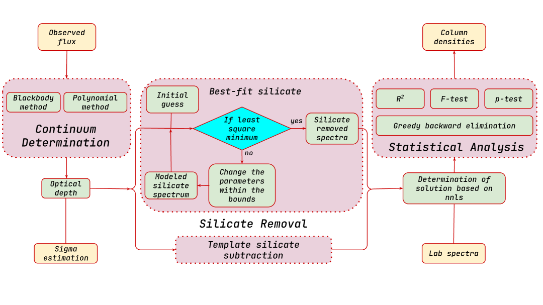
Figure 1: Schematic representation of the methodology for deriving the ice column densities using INDRA. The process includes continuum determination, followed by silicate feature removal and global ice fitting using NNLS. Statistical analysis is performed to assess fit quality and uncertainties after which final column densities are estimated.

3.1 Continuum removal

In order to constrain the ice absorption features and estimate accurate column densities, it is imperative to determine the continuum and remove it from the observed data before fitting for laboratory ices. However, accurately identifying the continuum SED poses several challenges, particularly in the wavelength range from 5 to 30 $\mu$m, where ice absorption features not only overlap with silicate features but also blend with other ice absorption bands. Additionally, the absorption bands can show a wide range of widths and shapes depending upon the local chemical inventory, further complicating the continuum determination. Rocha et al. (2021) have detailed some of the challenges in determining the continuum in this wavelength range. The continuum SED shortwards of 5 $\mu$m can be better constrained because of the lack of ice absorption features except for some narrow features of CO₂ and CO ices that appear at around 4.27 and 4.67 $\mu$m respectively. Several methods for constraining the continuum SED at these wavelengths have been documented in the literature. For example, continuum estimation using Kurucz stellar atmosphere models for wavelengths below 4 $\mu$m (Pontoppidan et al., 2004), and a linear combination of blackbodies to fit the near- and mid-infrared (IR) wavelengths (Ishii et al., 2002), can not only estimate the continuum SED but also constrain physical properties such as extinction and effective temperature.

In this study, we adopt the two continuum estimation methods between 5 and 30 $\mu$m proposed by Rocha et al. (2021). These two methods are:

(1) A polynomial approach, where a low-order polynomial given by Equation 1 is used to estimate the continuum:

$$F_{\text{poly}}(\lambda)=\sum_{k=0}^{n}a_{k}\lambda^{k}.$$ (1)

Here, $n$ is the order of the polynomial, $\lambda$ is the wavelength, and $a_{k}$ are the polynomial coefficients that determine the contribution of each power of wavelength to the overall continuum shape.

(2) A multi-temperature blackbody approach, where the continuum is modeled as a sum of blackbody curves, as described by Equation 2:

$$F_{\text{BB}}(\lambda,T)=\sum_{i=1}^{m}f_{i}\frac{2hc^{2}}{\lambda^{5}}\left(\frac{1}{\exp\left(\frac{hc}{\lambda k_{\text{B}}T_{i}}\right)-1}\right).$$ (2)

Here, $T_{i}$ is the temperature of the $i^{\text{th}}$ blackbody, $\lambda$ is the wavelength, $k_{\text{B}}$ is Boltzmann’s constant, $c$ is the speed of light, $h$ is Planck’s constant, and $f_{i}$ is a scaling factor.

To achieve continuum subtraction, the INDRA tool enables users to interactively select guiding points for polynomial continuum fitting. The tool then identifies the continuum based on these user-defined points and calculates the continuum SED. These guiding points serve as anchors for optical depth calculations. Once selected, the tool fits the continuum using a user-defined polynomial of finite order. It then calculates the optical depth using Equation 3, thereby consolidating the absorption features in optical depth scale.

$$\tau(\lambda)=-\ln\left(\frac{F_{\text{obs}}(\lambda)}{F_{\text{cont}}(\lambda)}\right)$$ (3)

3.2 Silicate feature removal

To isolate ice absorption features in the mid-infrared spectra, we remove the silicate contributions by modeling their synthetic optical depth, followed by baseline correction methods. This is necessary to address the overlapping silicate absorption bands around 9.8 $\mu$m and 18 $\mu$m with key ice features. Previous studies of protostars employed a silicate profile observed towards the galactic centre source (GCS 3) as a template (Boogert et al. 1997, Bottinelli et al. 2007). However silicate profiles can come in different shapes and sizes, and using GCS 3 as a template silicate may not completely remove the silicate features. Instead, it can introduce spurious features as demonstrated in figures A.1 and A.2 of Rocha et al. (2024). To overcome this limitation, INDRA tool offers two approaches to removing silicate features: one utilizing a predefined silicate model and another modeling the synthetic silicate spectra by exploring the silicate composition parameter space. Both approaches are discussed below.

3.2.1 Template silicate subtraction

In this approach, we use a predefined silicate absorption model derived from observational or laboratory data, or educated guess. The known silicate components are scaled to match the observed spectrum, ensuring that their contribution is accurately subtracted. This approach is particularly useful when the silicate composition is well-constrained, allowing for a straightforward removal of the silicate absorption without requiring extensive modeling. However, it requires a precise knowledge of the surface densities and compositions of different silicate components, and their mass fractions which is not always possible.

3.2.2 Synthetic silicate model

In the second approach, we explore the parameter space consisting of different silicate components with varying surface densities and mass fractions. We utilize the optool code (Dominik et al., 2021) to generate the optical depth spectra of the silicates. The silicate parameters that can be modelled using INDRA are shown in the Table 1.

Table 1: Silicate grain parameters

Parameter	Typical Values
Core composition	Pyroxene, Carbon etc.
Core mass fraction	Pyroxene (0.82), Carbon (0.18)
Surface density	$\sim$105 g cm-2
Mantle composition	H2O
Mantle fraction	0–0.5
Grain geometry	DHS, CDE
Porosity	0.8

Notes. DHS: Distribution of Hollow Spheres; CDE: Continuous Distribution of Ellipsoids. These grain geometries are used to model irregular silicate grain shapes.

To determine the synthetic silicate model, we simultaneously fit both the 9.8 $\mu$m and 18 $\mu$m bands. Once the synthetic silicate optical depths of different components are computed, a baseline correction is applied to each spectrum to remove any continuum variations or underlying broad features that could interfere with the fitting process. Following the baseline correction, the spectra are recombined using scaling factors applied to each silicate species to best match the observed data, and in particular to match the 9.8 $\mu$m and 18 $\mu$m absorption features. In this process, we optimize the scaling factors, the mass fractions of silicates and their surface densities using a non-linear least squares fitting procedure as shown in the Figure 1 and thereby determine the best fit for the silicate absorption profiles.

3.3 Laboratory ice data

The laboratory ice data used in INDRA consists of 772 ice spectra, provided in the format of wavenumber versus absorbance. The data are compiled from publicly available ice databases such as the Leiden Ice Database, the NASA Cosmic Ice Laboratory , UNIVAP and the Optical Constant Database that have comprehensive spectroscopic measurements of ices relevant to astrophysical environments. Some key ices include CO, H₂O, CH₄, NH₃, and organic molecules which have been observed in various astrophysical environments including low mass star forming regions. The spectra are measured in the laboratory under various physical conditions representing those of star-forming regions, providing us a wide range of data useful for ice fitting of YSOs. Before using the laboratory data in INDRA, we conducted a survey of the ices which are potentially contributing to the observed optical depths. This is because the spectra of same ice components are recorded at different temperatures. Though the band profiles are temperature-dependent, yet most absorption features remain largely unaffected posing a risk of overfitting if all the components are included. To mitigate this, we selected 76 components for the final fitting, the details of which are found in Appendix A. These spectra are essential for accurately fitting the observed ice absorption features. To ensure proper fitting, the spectra are preprocessed, which involves applying baseline corrections to select ice components to enhance the clarity of absorption features or to isolate minor component features that might otherwise be obscured by stronger ones. For this work, we correct the baselines of specific ice components, particularly those involving organic molecules in water mixtures where H₂O features dominate (see Appendix C). Once compiled, the data can be used in INDRA fitting, where we further normalize the laboratory spectra to facilitate comparison with observational data.

3.4 Ice fitting using weighted NNLS

This study employs a weighted Non-Negative Least Squares (weighted NNLS) algorithm to fit laboratory ice absorption spectra to the observed spectra of the YSO. The weighted-NNLS method ensures that all fitted coefficients remain non-negative, which is physically meaningful for the absorption spectra and ensures that the fitted components remain above the sigma noise estimate. The laboratory ice absorption spectra consist of several ices each with a distinct absorption profile. The observed spectrum can be modeled as a linear combination of these profiles scaled by appropriate non-negative coefficients. The weighted-NNLS method is applied to determine these scaling factors and thereby determining the contribution of each such ice to the absorption spectra. The following is a description of the algorithm.

Let the observed spectrum be represented as a vector $\mathbf{y}\in\mathbb{R}^{n}$ with each element $y_{i}$ corresponding to the observed flux at wavelength $\lambda_{i}$. Similarly let $\mathbf{A}\in\mathbb{R}^{n\times m}$ represent the matrix of laboratory ice absorption spectra where each column $\mathbf{A}_{j}$ is the absorption profile of a specific ice component. The objective of the fitting process is to find the non-negative coefficient vector $\mathbf{x}\in\mathbb{R}^{m}$ where each element $x_{j}$ represents the scaling factor of the corresponding ice component such that the residual between the observed and modeled spectrum is minimum.

The weighted-NNLS problem can be formulated as:

$$\min_{\mathbf{x}}\sum_{i=1}^{n}w_{i}^{2}\left(y_{i}-\sum_{j=1}^{m}A_{ij}x_{j}\right)^{2}$$ (4)

Here, $w_{i}$ is the weight given by $\frac{1}{\sigma_{i}}$, where $\sigma_{i}$ is the observational uncertainty at wavelength $\lambda_{i}$. The weighting ensures that data points with larger uncertainties have a smaller contribution to the total residual.

The NNLS algorithm solves for the minimization criteria given by Equation 4 subject to the constraint that $x_{j}\geq 0$ for all $j$. This ensures that the fit does not include any unphysical negative contributions from any of the ice components.

Convergence is reached when the residual cannot be reduced further while maintaining the non-negativity constraint on the coefficients. By using the weighted-NNLS method, we ensure that the laboratory ice absorption profiles are optimally scaled to match the observed spectrum, providing robust estimates of the ice column densities in the observed source.

3.5 Estimation of statistical significance

Accurate noise estimation is crucial in spectroscopic analysis, particularly when identifying weak absorption features in the optical depth spectrum and ascertaining the accuracy of the spectral fitting. A common approach, which has also been used by Rocha et al. (2024), is to assume a fixed 10% noise level across the spectrum. While this assumption may be reasonable for high-S/N spectra with uniform noise at all wavelengths, it does not account for variations in baseline fluctuations, instrumental response or wavelength-dependent noise. Consequently, such a fixed uncertainty can lead to either an over-estimation or under-estimation of the actual noise, potentially affecting the reliability of spectral fits. To obtain a more accurate estimate of the noise, we employ a polynomial-based approach similar to that of Chen et al. (2024). Instead of assuming a fixed percentage, the noise level is estimated at multiple spectral regions devoid of strong absorption features, and an average value is taken across these regions. Appropriate polynomials are used to model and subtract the baseline fluctuations, ensuring that the noise estimation reflects the true uncertainties in the data. The noise level at each region is calculated using:

$$\sigma=\sqrt{\frac{\sum_{i=1}^{N}(y_{i}-\bar{y})^{2}}{N}}$$ (5)

where $y_{i}$ represents the polynomial-subtracted optical depth at each spectral channel within the selected region, and $\bar{y}$ is the mean value of $y_{i}$. This method provides a robust uncertainty estimate, crucial for assessing the significance of weak absorption features and the reliability of the fits. By averaging over multiple regions, it captures the global noise characteristics across the wavelength range rather than relying on a single estimate. The computed noise level is then incorporated into our statistical analysis to ensure a reliable interpretation of the spectral fits.

3.5.1 Greedy backward elimination as a check against overfitting

As a check against overfitting, we use the greedy backward elimination approach based on a chi-square statistical evaluation using the Equation 6:

$$\chi^{2}=\sum_{i}\frac{(O_{i}-E_{i})^{2}}{\sigma_{i}^{2}},$$ (6)

with $O_{i}$ representing the observed data points, $E_{i}$ the model values for those data points, $\sigma_{i}$ the estimated uncertainty given by Equation 5. This method iteratively removes each component from the model while preserving the rest and evaluates the $\chi^{2}$ value to assess the goodness of fit. At each step, we systematically remove one component at a time and fit the rest of the components using weighted-NNLS. The component whose removal results in the smallest increase in $\chi^{2}$ is identified as the least significant and is tentatively eliminated. To ensure that the removal of a component does not degrade the overall fit, we compute the p-value associated with the change using the $\chi^{2}$ distribution. The p-value quantifies the probability of obtaining a $\chi^{2}$ difference as extreme as observed, assuming that the removed component does not significantly contribute to the fit. Mathematically, the p-value is derived from the cumulative distribution function (CDF) of the $\chi^{2}$ distribution:

$$p=1-F_{\chi^{2}}(\Delta\chi^{2},\nu)$$ (7)

where $\Delta\chi^{2}=\chi^{2}_{\text{before}}-\chi^{2}_{\text{after}}$ is the change in chi-square upon removing the component, and $\nu=d_{\text{before}}-d_{\text{after}}$ is the difference in degrees of freedom. The function $F_{\chi^{2}}(\Delta\chi^{2},\nu)$ represents the cumulative probability of observing a chi-square value up to $\Delta\chi^{2}$ under the null hypothesis. A high p-value ($p>0.05$) suggests that the difference in chi-square is small and likely due to random fluctuations rather than a meaningful improvement in fit. In this case, the removed component is deemed statistically insignificant, justifying its elimination. Conversely, if the p-value falls below a predefined threshold ($p\leq 0.05$), the change in chi-square is large enough to indicate that the removed component significantly contributes to the model, and it should be retained. By evaluating the statistical significance of component removal using p-values, we ensure that only the most relevant components are retained in the fit, thereby preventing overfitting while maintaining an optimal representation of the observed data.

3.5.2 R² statistic to assess the goodness-of-fit

The goodness-of-fit is assessed using the coefficient of determination ($R^{2}$), which quantifies how well the model explains the variance in the observed data as each component is being added. It is given by:

$$R^{2}=1-\frac{\sum_{i=1}^{n}(y_{i}-\hat{y}_{i})^{2}}{\sum_{i=1}^{n}(y_{i}-\bar{y})^{2}}$$ (8)

where $y_{i}$ are the observed values, $\hat{y}_{i}$ are the model-predicted values, and $\bar{y}$ is the mean of the observed data. An $R^{2}$ value close to 1 indicates that the model explains most of the variance in the data, while a value near 0 suggests poor explanatory power. While calculating the R² statistic as each component is added, we consider only its contributing region, defined as the wavelength range where the component’s contribution exceeds the sigma level calculated for the source.

3.5.3 F statistic to evaluate the relevance of minor components

We note that chi-square values may not accurately capture the significance of the components particularly when they are minor. To assess the statistical significance of individual minor ice components in our spectral fitting analysis, we performed an F-test, which evaluates whether the inclusion of that specific component significantly improves the model fit. The F-value is computed using Equation 9 for each component:

$$F=\frac{\left(\frac{\text{RSS}_{\text{test}}-\text{RSS}_{\text{full}}}{\text{df}_{\text{test}}-\text{df}_{\text{full}}}\right)}{\left(\frac{\text{RSS}_{\text{full}}}{N-\text{df}_{\text{full}}}\right)}$$ (9)

where $\text{RSS}_{\text{full}}$ is the residual sum of squares (RSS) for the full model (including the tested component), $\text{RSS}_{\text{test}}$ is the RSS for the reduced model (excluding the tested component), $\text{df}_{\text{full}}$ and $\text{df}_{\text{test}}$ are the degrees of freedom of the full and reduced models, respectively, and $N$ is the total number of data points. The F-values are computed as the ratio of the variance explained by each component to the residual variance and indicate the relative contribution of each component to the overall fit. Note that we use only the relevant wavelength window of each component specific to its contribution to the fitting. A higher F-value indicates that the tested component significantly improves the fit by reducing the residual variance in that wavelength window. Empirical thresholds for spectral fitting applications suggest the following classification of F-values:

• Strong contribution: $F>10$

• Moderate contribution: $2<F<10$

• Weak contribution: $F<2$

We note that these ranges are not strictly defined, and their interpretation depends on the sample size, degrees of freedom, etc.

The statistical significance of each component is further evaluated using the corresponding p-value, which represents the probability of obtaining an F-statistic as extreme as observed under the null hypothesis. This time the p-value is computed as:

$$p=P(F>F_{\text{obs}})$$ (10)

where $F_{\text{obs}}$ is the observed F-statistic. A lower p-value (typically $p<0.05$) suggests that the inclusion of the component significantly improves the model.

3.5.4 Estimation of confidence intervals

To quantify uncertainties in the best-fit coefficients for the ice absorption modeling and to estimate confidence intervals in the column densities, we generate perturbed coefficients by sampling values linearly spaced around each best-fit coefficient. Specifically, for each coefficient $C_{i}$, perturbed values were sampled uniformly between $C_{i}-\epsilon C_{i}$ and $C_{i}+\epsilon C_{i}$, where $\epsilon$ is a fractional error factor defining the perturbation range.

For each perturbed coefficient set, a synthetic spectrum $y_{\mathrm{model}}$ was generated, and its fit to the observed optical depth spectrum $y_{\mathrm{obs}}$ is evaluated using the normalized chi-square statistic given by:

$$\chi^{2}_{\mathrm{norm}}=\frac{\sum\left(\frac{y_{\mathrm{obs}}-y_{\mathrm{model}}}{\sigma_{y}}\right)^{2}}{\sum y_{\mathrm{model}}^{2}},$$ (11)

where $\sigma_{y}$ is the observational uncertainty.

Confidence intervals are then determined for each coefficient by identifying the range of $C_{i}$ values corresponding to an acceptable increase in $\chi^{2}_{\mathrm{norm}}$. The lower and upper bounds in the coefficients are then used to calculate the minimum and maximum optical depths, setting limits on the column densities for each ice, computed as described in Section 3.6.

The correlations between different ice components vary with wavelength due to the presence of complex mixtures, which can induce shifts in absorption band positions and alter band shapes. As a result, uncertainties and parameter correlations are not uniform across the spectral range, and a global analysis may not effectively capture these localized effects. Therefore, we perform the analysis in a sliding-window, local manner across the spectrum to account for wavelength-dependent uncertainties. This localized approach enables robust estimation of coefficient significance, their correlations, and the associated error bars in the derived column densities.

For each coefficient, the overall lower bound is taken as the minimum of all lower bounds obtained from individual sliding windows, while the overall upper bound is taken as the maximum of all upper bounds from these windows. This method ensures a comprehensive estimation of the confidence intervals.

3.6 Column density estimation

Once the best fit solution is found, we calculate the column density of each ice using Equation 12,

$$N_{\text{ice}}=\frac{1}{A}\int_{\nu_{1}}^{\nu_{2}}\tau_{\text{lab}}(\nu)d\nu$$ (12)

where $A$ represents the vibrational mode band strength of the molecule. The band strengths vary with the chemical environment, making their accurate determination crucial for reliable column density estimates. While calculating the column densities, we incorporate corrected band strength values from the literature. The appendix Table B provides the list of all the band strengths used in this work. It is to be noted that derivation of band strengths is inherently dependent on ice density, leading to typical uncertainties of approximately 15% for pure ices and 30% for mixed ices (Rachid et al. 2022; Slavicinska et al. 2023).

4 Results

In this section we present the fitting results for IRAS 2A across the entire MIRI wavelength range (5–28 $\mu$m). This includes the continuum removal, silicate subtraction, global ice fitting, statistical analysis and the final estimation of ice column densities. Additionally, we compare our results with previous study that employed a local fitting approach.

4.1 Continnum determination in IRAS 2A

The continuum fit and the corresponding optical depths of the source IRAS 2A are presented in Figure 2. The continuum and the optical depths calculated by Rocha et al. (2024) are also presented for a comparison. The SED of IRAS 2A is characteristic of embedded protostars, both high-mass and low-mass, exhibiting an increasing slope toward longer wavelengths (Gibb et al. 2004, Boogert et al. 2008). The observed SED can be modeled using a blackbody approach, assuming contributions from warm dust at wavelengths shorter than 20 $\mu$m and cold envelope material at longer wavelengths. However, in this work, a third-order guided polynomial is used to determine the continuum.

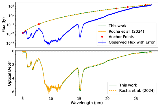
Figure 2: Continuum determination in the source IRAS 2A. The top panel displays the observed flux (blue) on a logarithmic scale, along with the continuum (green) traced using a guided polynomial fit. The anchor points used for continuum fitting are marked as red dots. The bottom panel presents the corresponding estimated optical depths (green). For comparison, data from Rocha et al. 2024 is also plotted (orange).

This choice is motivated by several factors: (1) the lack of reliable constraints on the temperature components required for blackbody modeling, (2) the flexibility of the polynomial approach in tracing complex absorption features across MIRI, and (3) to maintain consistency with the continuum shape adopted in Rocha et al. (2024), enabling a direct comparison of the resulting ice column densities and evaluation of how different fitting methods influence the derived ice column densities. We use anchor points to trace the continuum and the same are shown in Figure 2. Please note that some points were placed slightly above the observed data to better approximate the continuum used in the earlier study. However, we emphasize that significant uncertainties are inherently associated with the choice of the continuum, as silicate absorption can extend to longer wavelengths making it challenging to trace it accurately. A detailed treatment of this continuum ambiguity is beyond the scope of the present work. Once the continuum is traced, we convert the spectra into optical depth units using Equation 3.

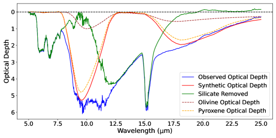
Figure 3: Silicate removal in the source IRAS 2A. The observed optical depth spectrum is shown in blue, while the modeled silicate absorption is represented by the solid red line. The individual silicate components contributing to the overall absorption are olivine (dotted brown) and pyroxene (dotted orange). The final silicate-subtracted spectrum is shown in green.

4.2 Silicate feature removal in IRAS 2A

The spectrum of IRAS 2A in optical depth units is shown in the bottom panel of Figure 2. Broad silicate absorption features are prominent around 9.8 $\mu$m and 18 $\mu$m, partially overlapping with the absorption bands of organic ices and H₂O-CO₂ respectively. In particular, organic ice absorption features embedded within the 9.8 $\mu$m region become more distinct once the silicate features and local continuum are removed (Rocha et al., 2024). Additionally, the true shape of the CO₂ band at $\sim$15 $\mu$m emerges more clearly after accounting for the overlapping silicate feature near 18 $\mu$m. The silicate removed spectra of IRAS 2A is shown in Figure 3. For this work, we adopt a template silicate subtraction method, leveraging the well-constrained silicate model from Rocha et al. (2024) to ensure consistency and accuracy in isolating the ice absorption features. Briefly, the template silicate model consists of two components: amorphous pyroxene (Mg_0.5Fe_0.5SiO₃) and olivine (MgFeSiO₄). Each of these component is assumed to be mixed with carbon, a common constituent of interstellar grains. The volume fractions of silicate and carbon are set to 82% and 18% respectively. This approach is in line with various protostellar and diffuse interstellar medium models, where carbon fractions can vary between 15 and 30% (Woitke et al. 2016; Pontoppidan et al. 2005; Weingartner & Draine 2001). The grain size distribution is modeled using a power-law size distribution with an exponent of 3.5, and grain sizes ranging from 0.1 to 1 $\mu$m, consistent with interstellar grain models. To account for the irregular geometry of the dust grains, we adopt a distribution of hollow spheres, a method that provides more realistic fits to the silicate absorption features than simple spherical grain models.

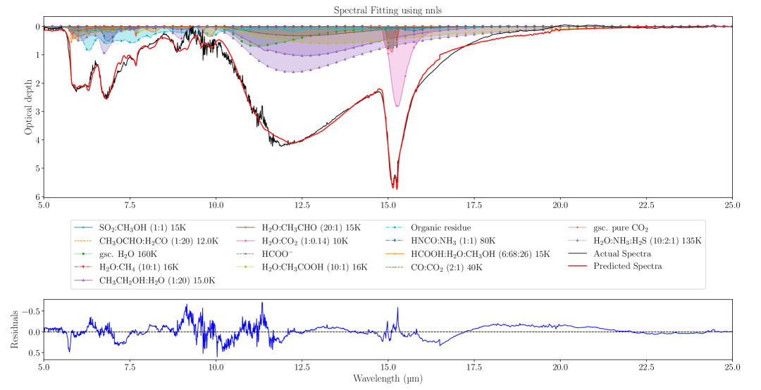
Figure 4: Global ice-fitting results across the entire MIRI spectrum (5–25 $\mu$m). The top panel shows the observed optical depth spectrum (solid black) alongside the modeled optical depth spectrum (solid red), which represents the contribution from 15 best-fit ice components. Each contributing component is displayed using different colors, markers, and line styles and are mentioned in the middle panel as a legend. The bottom panel presents the residuals corresponding to the fit.

4.3 INDRA global fitting results

The MIRI spectrum of IRAS 2A shows a high S/N and distinct absorption features spanning 5–28 $\mu$m. At shorter wavelengths $\lesssim$ (10 $\mu$m), the spectrum is primarily shaped by absorption from H₂O, organic molecules and organic refractory materials, and silicates. At longer wavelengths ($\gtrsim$ 10 $\mu$m), strong absorptions from H₂O, CO₂, and silicates dominate the spectrum. By subtracting the silicate contributions, the remaining absorption features between 5 and 20 $\mu$m can be primarily attributed to ices. The fitting results for the entire MIRI wavelength range of the source IRAS 2A is shown in Figure 4. Our spectral fitting analysis reveals the presence of multiple ice components including simple species such as H₂O, CO₂, CH₄ as well as COMs like CH₃OH, CH₃CH₂OH, etc. Rocha et al. (2024) carried out local fitting in the COMs finger-print region (6.8 - 8.6 $\mu$m) of the source and estimated the column densities of COMs present in that region along with H₂O. In this work, we analyze the entire MIRI spectrum and decompose it using a laboratory ice database containing 76 ices, out of which 15 contribute to the global minimum solution. Each of these 15 components shows a peak optical depth that exceeds the noise level in the observed spectrum, indicating appreciable contributions. Their statistical significance are evaluated in Section 4.4.

4.3.1 Absorption bands of simple ices H₂O, CO₂, NH₃, SO₂

The MIRI spectra of IRAS 2A show broad absorption features of H₂O due to the bending mode at around 6 $\mu$m and the libration mode at around 13 $\mu$m. The 6 $\mu$m region is particularly complex due to significant overlap with absorption features from COMs and other simple molecules. Similarly, the 13 $\mu$m region coincides with strong absorption from silicates and CO₂, resulting in blended features that require a combination of pure and mixed ice components for spectral decomposition. The top right panel in Figure 5 shows the H₂O and CO₂ related best-fit components. All these components are dominant in nature and contribute much to the shape of the overall spectra. H₂O ice appears in both pure and mixed forms, contributing to the bending mode at $\sim$6 $\mu$m and the libration mode at $\sim$13 $\mu$m. We apply grain shape correction to the 160 K pure H₂O ice using Mie theory and assuming small grains where it shows a blue wing excess in the 13 $\mu$m libration band.

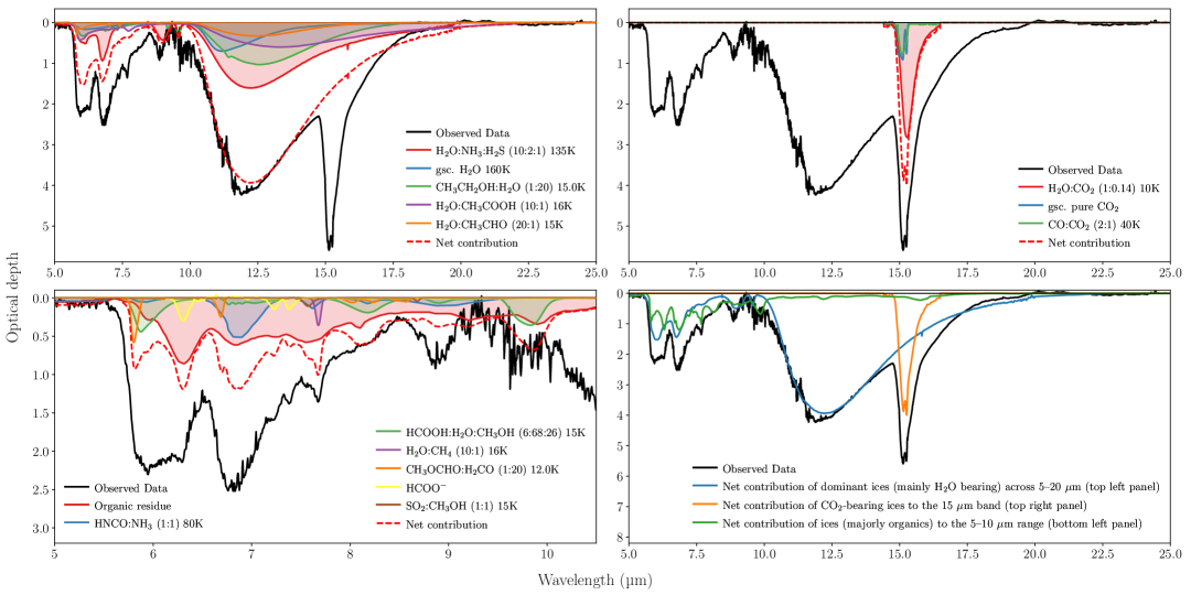
Figure 5: Best-fit decomposition of the MIRI spectrum of IRAS 2A, highlighting the contributions from different ice and organic components. The observed optical depth spectrum is shown in solid black across all panels. Top-left panel: Contributions from H₂O and CO₂ ices, which are the dominant components in the spectrum. The individual ice components are plotted in solid colors, while their cumulative contribution to the observed spectrum is shown in dotted red. Top-right panel: Contributions from organic residues, another dominant component, shown in blue. Bottom-left panel: Contributions from organic molecules, including CH₃OH, H₂CO, CH₄, and other complex organic species. As in the previous panels, each component is shown in solid colors, and their combined contribution on the overall spectrum is in dotted red. Bottom-right panel: A summary panel showing the individual contributions to the observed spectrum from the three categories: H₂O-CO₂ ices, organic residues, and organic molecules.

Similarly, the MIRI spectrum of IRAS 2A has a distinct absorption at 15 $\mu$m due to CO₂ . CO₂ ice appears both in its pure form and as part of mixed ice components. The following components are used to fit the spectrum: pure CO₂ ice, 40 K ice mixture CO: CO₂ in 2:1 ratio, 10 K ice mixture H₂O: CO₂ in 1:0.14 ratio. Similar ice components were used by Pontoppidan et al. (2008) and Rocha et al. (2025). The observed double peak in the 15 $\mu$m band is likely a result of ice distillation or segregation due to thermal processing and is well fit by pure CO₂ ice. This component shows a prominent blue wing, contributing to the shortward side of 15 $\mu$m band, whereas the 10 K H₂O:CO₂ ice mixture contributes to the red wing of this band. Both Pontoppidan et al. (2008) and Rocha et al. (2025) found CO₂ ice in H₂O ice-rich environments, which is also the case in the present work. Additionally, contributions from CO ice dominated regions play a role.

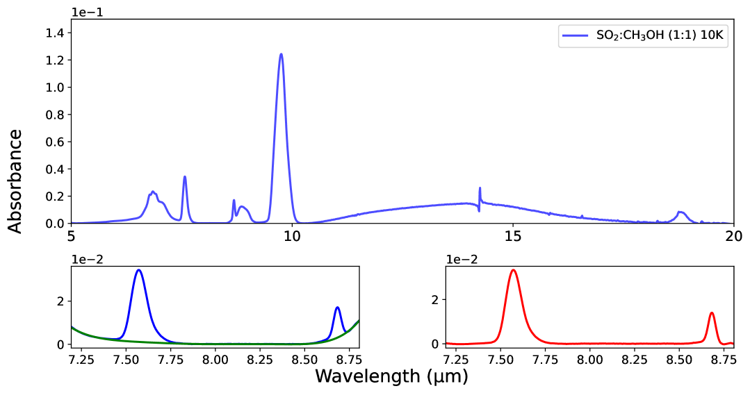
Figure 15: The absorption profile of SO₂:CH₃OH (1:1) 10 K ice mixture is shown in blue. The bottom-left panel shows the SO₂ features at 7.57 and 8.68 $\mu$m in blue and the corresponding local polynomial baseline in green. The resultant baseline-corrected profiles are shown in red in bottom-right panel.

Sulfur dioxide (SO₂) shows strong absorption features in the mid-infrared (MIR) region, particularly near 7.7 and 8.5 $\mu$m, which correspond to its asymmetric ($\nu_{3}$) and symmetric ($\nu_{1}$) stretching modes, respectively. We isolated both these bands of SO₂ from a mixture SO₂:CH₃OH as shown in the Figure 15. Ammonia (NH₃) is also found in the fits. The absorption band at 8.9 $\mu$m in the observed optical depth spectrum can be related to this ice. Two ice components as shown in Table 2 carry this band in the fits with the H₂O:H₂S based mixture showing significant contribution to the 8.9 $\mu$m band. Notably, this region also overlaps with some minor bands from CH₃CH₂OH, CH₃OH, CH₃CHO, and SO₂, which can lead to blending and complex shape to the optical depth spectrum. The deviation between the model and the observations in this region may be due to uncertainties in the organic refractory baseline, the placement of the global continuum, the silicate subtraction, or a combination of these factors.

Table 2: Ice mixtures containing H₂O, CO₂, and SO₂

Ice Mixture	Ratio	T (K)
H2O components
H2O:NH3:H2S	10:2:1	135
CH3CH2OH:H2O	1:20	15
H2O:CH3COOH	10:1	16
H2O:CH3CHO	20:1	15
Pure gsc. H2O	—	160
CO2 components
H2O:CO2	1:0.14	10
CO:CO2	2:1	40
Pure gsc. CO2	—	—
SO2 component
SO2:CH3OH	1:1	10
NH3 component
H2O:NH3:H2S	10:2:1	135
NH3:HNCO†	1:1	80

Note: gsc. denotes a grain shape–corrected component; $\dagger$ denotes the spectrum of the residual component. For references, see Appendix A.

4.3.2 Absorption bands of NH${}_{4}^{+}$, OCN^- and HCOO^- ion salts

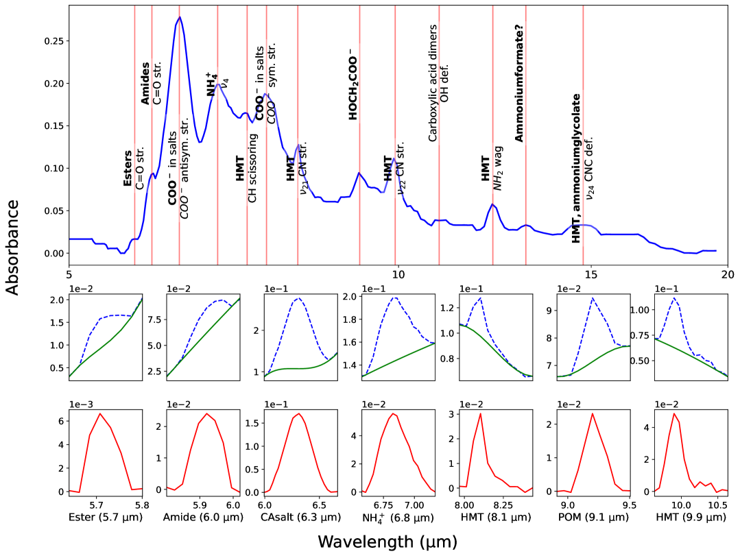
Figure 12: IR spectrum of the residue (blue) of the irradiated ice mixture H₂O:NH₃:CH₃OH:CO:CO₂ (2:1:1:1:1) at 12 K (Muñoz Caro & Schutte, 2003) in the wavelength region 5–20 $\mu$m shown in the top panel. Note the absorption features of key refractory species, as indicated by the intersections of the red vertical lines with the blue spectrum. These features correspond to various functional groups, including carbonyl (-C=O), carboxylate (-COO^-), amine (-NH₂), and -CN containing species. Also, note that these absorption features are blended in a broad profile requiring us to estimate local baseline for the calculation of column densities. The middle panel of the figure shows the portion of the spectrum (blue) where features due to various functional groups appear and their corresponding local polynomial baseline (green). The baseline-corrected features are shown in red in the bottom panel. Column densities are estimated using Equation 12 and band strengths mentioned in Appendix B.

Table 3 lists all the ice components that show the spectral features of ions. In our global fitting results, we found the Ammonium ion (NH${}_{4}^{+}$) in three distinct ice components: within the NH₃:HNCO ice residue that is responsible for OCN^- ion, in the H₂O:NH₃:CH₃OH:CO:CO₂ ice residue that is responsible for the organic residue shown in Figure 12 and the H₂O:NH₃:H₂S (10:2:1) ice mixture at 135 K. The 6.7 $\mu$m band of these ice components can be assigned to the $\nu_{4}$ mode of NH${}_{4}^{+}$ (Wagner & Hornig, 1950). The broad absorption dip centered around 6.6 $\mu$m in the observed optical depth spectrum of IRAS 2A is well explained by these three components, and the model provides an excellent agreement with the data in this region.

Table 3: Ice mixtures containing ion salts

Ice Mixture	Ratio	T (K)	Species
H2O:NH3:H2S	10:2:1	135	H2O, NH${}_{4}^{+}$, NH3
NH3:HNCO†	1:1	80	OCN-, NH${}_{4}^{+}$, NH3
H2O:NH3:CH3OH:CO:CO${}_{2}^{\dagger}$	—	—	NH${}_{4}^{+}$
H2O:NH3:HCOOH†	100:2.6:2	14	HCOO-

Note: $\dagger$ denotes spectra of the residual components. (For references, see Appendix A.)

Of all the components, Cynate ion (OCN^-) contributes to several bands in the 5-10 $\mu$m region and to the $\sim$ 15 $\mu$m band. The spectrum of this ion salt was obtained by Novozamsky et al. (2001) using an 80 K ice mixture of NH₃:HNCO in 1:1 ratio. The spectral evolution of the mixture when it is gradually being warmed, reveals features at approximately 6.67, 7.72, 8.26, and 15.87 $\mu$m, which are not associated with the original species. As the temperature increases, these bands grow in intensity while the characteristic bands of HNCO and NH₃ diminish, indicating proton transfer between HNCO and NH₃. The band at 6.67 $\mu$m corresponds to the vibrational mode of NH${}_{4}^{+}$, whereas the features at 7.72, 8.26, and 15.87 $\mu$m are assigned to OCN^-.

Another ion identified in our fitting is Formate ion (HCOO^-), which contributes to the bands at 6.32, 7.24, and 7.40 $\mu$m. This result is consistent with the findings of Rocha et al. (2024). The spectrum is obtained using the hyper-quenching technique on NH₄COOH salts obatined via acid base reactions involving the 14 K ice mixture of H₂O:NH₃:HCOOH in a ratio 100:2.6:2 (Gálvez et al., 2010). To analyze the HCOO^-, we isolated its ice bands using a local baseline subtraction method. HCOO^- exhibits a strong band at 6.32 $\mu$m, which blends with the intense H₂O absorption at 6 $\mu$m, contributing to the excess in this region. Additionally, its 7.2 $\mu$m band overlaps with contributions from HCOOH. Therefore, the 7.4 $\mu$m band is used to estimate HCOO^- column densities.

4.3.3 Absorption bands of organic molecules

The Table 4 summarizes the organic ice components appearing in the fitting. Components where the H₂O bands are retained as mentioned in Table 4 are shown in the top left panel of the Figure 5 and the mixtures where H₂O bands are removed (refer to the Appendix C) are shown in the bottom left panel of the figure to aid visual inspection. All the organic molecules with secure and tentative detections as reported in Rocha et al. (2024) are found in this work.

Table 4: Organic ice mixtures appearing in the fitting

Ice Mixture	Ratio	T (K)	H2O Bands
H2O:CH4	10:1	16	Removed
HCOOH:H2O:CH3OH	6:68:26	15	Removed
CH3OCHO:H2CO	1:20	12	—
CH3CH2OH:H2O	1:20	15	Retained
H2O:CH3COOH	10:1	16	Retained
H2O:CH3CHO	20:1	15	Retained

Note: See Section 5.2 and Appendix C for more on H₂O band removal. (References in Appendix A)

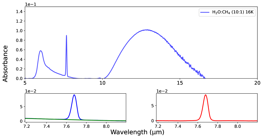
Figure 13: The absorption profile of H₂O : CH₄ (10:1) ice mixture (Rocha et al., 2017) is shown in blue. The bottom-left shows the CH₄ bending mode at 7.6 $\mu$m in blue and the corresponding local polynomial baseline in green. The resultant isolated band of CH₄ is shown in red.

In our analysis, the observed absorption excess at 7.7 $\mu$m is attributed to Methane (CH₄), which is present in the fits as an H₂O:CH₄ ice mixture. CH₄ has a band at $\sim$ 7.7 $\mu$m as shown in Figure 13. Due to the interaction with H₂O, CH₄ shows band broadening, leading to a better match with observations when this mixture is considered alongside the OCN^-, SO₂ and CH₃COOH ice bands in the region. An absorption excess in the blue wing of the band is primarily due to OCN^-, and SO₂ whereas CH₃COOH contributes to the red wing of the band.

In our fits, Formic acid (HCOOH) appears as a HCOOH:H₂O:CH₃OH ice mixture which contributes to several absorption features across the MIRI range, including distinct bands at 5.83 $\mu$m ($\nu_{S}$(C=O)), 6.06 $\mu$m ($\nu_{S}$(C=O)), 7.21 $\mu$m ($\nu_{B}$(OH) & $\nu_{B}$(CH)), 8.26 $\mu$m ($\nu_{S}$(C–O)), 9.32 $\mu$m ($\nu_{B}$(CH)), 10.75 $\mu$m ($\nu_{B}$(OH)), and 14.18 $\mu$m ($\nu_{B}$(OCO)). Additionally, HCOOH’s interaction with H₂O results in feature at 5.88 $\mu$m. Blending effects arise due to the presence of other species in the mixture. Methanol (CH₃OH) shows absorption bands at 6.85, 8.85, and 9.75 $\mu$m, overlapping with HCOOH features and contributing to the complexity of the spectrum. The band at 9.74 $\mu$m is due to the C-O stretch and fits well within the observed spectrum. This band falls in a region where the absorption band is saturated and a factor multiplication of 2 is applied to the column density estimations which is also aligned with Rocha et al. (2024). The deviation between the model and the observed optical depth spectrum around 8.26 $\mu$m region may be due to the uncertainties in the refractory material baseline, the placement of the global continuum or any combination of these factors.

Methylformate (CH₃OCHO) appears as a mixture with H₂CO in the fits. Its pure form shows vibrational bands at 5.8 $\mu$m (C=O stretch), 8.26 $\mu$m (C–O stretch), 8.58 $\mu$m (CH₃ rocking), 10.98 $\mu$m (O–CH₃ stretch), and 13.02 $\mu$m (OCO deformation) (Terwisscha van Scheltinga et al., 2021). However, in the CH₃OCHO:H₂CO mixture, matrix interactions lead to band shifts and altered widths. The O–CH₃ stretching mode is blue-shifted, and the OCO deformation mode also shifts in position. The CH₃ rocking mode at 8.58 $\mu$m overlaps with the CH₂ wagging mode of H₂CO at 8.49 $\mu$m, producing a blended, broader feature in this region. The C=O stretch at 5.8 $\mu$m overlaps with the strong H₂CO band, making it unreliable for column density estimation. Instead, the relatively stable C–O stretching mode at 8.26 $\mu$m is used to determine the column density of CH₃OCHO. The H₂CO column density is estimated using its feature near 8.02 $\mu$m.

Ethanol (CH₃CH₂OH) is identified in our fits as a H₂O mixture. The weaker vibrational modes at 7.24 $\mu$m (CH₃ symmetric deformation), 7.4–7.7 $\mu$m (OH deformation), and 7.85 $\mu$m (CH₂ torsion) fall in relatively clean spectral regions. However, its stronger bands at 9.17 $\mu$m (CH₃ rocking), 9.51 $\mu$m (CO stretch), and 11.36 $\mu$m (CC stretch) are blended with dominant ice features of H₂O, as well as the broad silicate feature at $\sim$9.7 $\mu$m. The 7.24 $\mu$m band of ethanol-water mixture is relatively easy to detect as H₂O induces a peak shift, making it a promising candidate for identification (Terwisscha van Scheltinga et al., 2018).

Acetic acid (CH₃COOH) shows absorption bands at 7.3 $\mu$m and 7.7 $\mu$m. In our fits, it appears as a mixture with H₂O, resulting in a broadened profile at 7.7 $\mu$m. This band overlaps to certain extent with the some bands of OCN^-, SO₂, CH₄, CH₃OCHO, CH₃CH₂OH and HCOOH whereas 7.3 $\mu$m falls rather in a clean region. However, the intensity of the 7.7 $\mu$m band is twice that of the 7.3 $\mu$m band and is used to determine its column density.

Acetaldehyde (CH₃CHO) is detected in our fits as part of an H₂O mixture in the ratio 1:10. It shows four significant absorption features in the 5.5–12.5 $\mu$m range, with the most prominent being the CO stretching mode at 5.8 $\mu$m. However, this band overlaps with other interstellar molecules like H₂CO, HCOOH, and NH₂CHO, making its identification challenging. Similarly, the 6.995 and 8.909 $\mu$m bands coincide with CH₃OH features, further complicating detection. The CH₃ symmetric deformation + CH wagging mode at 7.427 $\mu$m, which has minimal overlap with common ice components, is the most reliable for identifying it and the same is used to calculate the column density.

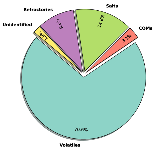
Figure 6: Percentage contribution to the spectral area of different ice groups in the 5–8 $\mu$m range. The model provides a good fit across the region as shown in the Figure 4, except for the 7.1–7.5 $\mu$m interval. Appropriate polynomial baselines are used to separate the different ice groups present in the same ice mixture.

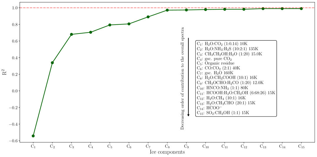
Figure 7: R² value as each component is added to the model. The R² for individual components is shown in green dots. The cumulative R², the normalized sum of cumulative R², is also plotted in blue dots to illustrate the relative change in R². Components are added in descending order of their contribution, which is defined as the maximum optical depth of the respective component.

4.3.4 Organic refractories

The bottom left panel in Figure 5 shows the significant presence of organic refractory materials, which contribute to the excess absorption dip in the 5–10 $\mu$m region of the observed optical depth, alongside the H₂O bending mode. These materials are refractories even at room temperature, having high molecular mass up to 200 amu, and contain several molecules, radicals, and other fragments. The organic refractories show broad absorption features spanning from $\sim$5.5 $\mu$m to $\sim$11 $\mu$m in the MIRI range, indicating the presence of various functional groups including carbonyl (C=O), hydroxyl (O-H), amine (N-H), and C-H bending modes. Notably, this spectral region also coincides with absorption bands of volatile organics such as COMs, including aldehydes, esters, carboxylic acids, and amides, leading to significant spectral blending. The overlapping absorption features contribute to the overall depth of the observed bands making it challenging to isolate individual molecular contributions. This necessitates the determination of the local continuum in order to accurately isolate the absorption features of volatiles which is shown in Rocha et al. (2024).

The spectra of organic refractories are obtained by Muñoz Caro & Schutte (2003) who irradiated 12 K mixture of H₂O:NH₃:CH₃OH:CO:CO₂ in the ratio 2:1:1:1:1 using an hard UV dose of 0.25 photon molec^-1. The residue spectrum is shown in Figure 12. The strongest peak due to the -COO^- antisymmetric stretch of carboxylic acid salts [(R-COO^-)(NH${}_{4}^{+}$)] is observed at around 6.3 $\mu$m. Hexamethylenetetramine (HMT) is also identified through the 8.10 ($\nu_{22}$) and 9.93 ($\nu_{21}$) $\mu$m stretch of CN. The peak at 9.21 $\mu$m characteristic of glycolic acid is due to ammonium glycolate. It also accounts for the 20% of the feature present at 6.30 $\mu$m due to the COO^- stretching mode. The rest is due to other acid salts like ammonium glycerate (HOCH₂CH(OH)COO^-)(NH${}_{4}^{+}$) and ammonium oxamate (NH₂COCOO^-)(NH${}_{4}^{+}$). The minor absorption features at 5.74 $\mu$m and 5.95 $\mu$m are attributed to the C=O stretching mode of esters (R–C(=O)–O–R${}^{{}^{\prime}}$) and primary amides (R–C(=O)–NH₂), respectively. A weak band due to NH₂ deformation in primary amides arises between 6.06–6.17 $\mu$m confirms the presence of primary amides.

The model, which includes refractory material spectra, accurately reproduces the observed absorption features in the 5–10 $\mu$m region, particularly between 5 and 7.12  $\mu$m, with the exception of some localized mismatches between 7.1–7.5  $\mu$m and at 8.26 and 8.9  $\mu$m. We suspect the mismatch in the 7.1–7.5  $\mu$m region may arise from unidentified or missing components. Similarly, the deviations observed at 8.26 and 8.9 $\mu$m may be due to uncertainties in the baseline of refractory material spectra. To better understand the relative contributions of refractory materials and various ice types to the 5–8 $\mu$m optical depth spectrum, we estimate the percentage area covered by each ice group, as illustrated in Figure 6. Volatile ices dominate the absorption area (70.6%), followed by salts (14.8%), refractory organics (9.6%), COMs (3.1%), and unidentified components constitute (1.9%). These findings highlight the importance of including organic refractory materials in the model to accurately reproduce the observed spectrum. The implications of refractory materials in astrophysical environments, including their formation efficiencies, are discussed further in Section 5.

4.4 Statistical interpretation

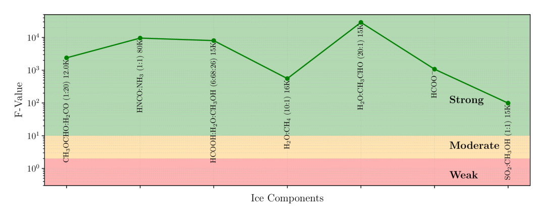
Figure 8: F-values for each minor ice component as it is sequentially added to the model, illustrating the relative change in variance. A higher F-value signifies a greater contribution of that component to the overall fit. Components are categorized as strong (in green region), moderate (in yellow region), or weak (in red region) based on the relative change in variance.

Figure 7 presents the R² analysis of the spectral fitting process, where components are added sequentially in descending order of their contribution, defined by the maximum optical depth of each component in the MIRI range. As shown in Figure 7, the first few components—mainly H₂O and CO₂ mixtures, along with organic residues—play a dominant role in improving the fit, leading to a rapid increase in the R² value. These species are expected to be major constituents of interstellar and protostellar ices due to their observed abundance in astrophysical environments. The model accuracy improves significantly till the first eight components whose contribution to the optical depth spectrum exceeds at least 0.6 in optical depth units. Beyond this point, adding relatively minor components (contributing $\lesssim$ 0.6 optical depth units to the spectrum) yields only marginal improvements, indicating that the overall spectral profile is largely governed by a few dominant species.

To assess the significance of these minor components, we performed Greedy Backward Elimination, F-tests, and p-tests. Among the 15 components included in the best-fit model, 8 are dominant, while the remaining ones contribute mostly to localized features. As evident from Figure 7, the R² value stabilizes after the eighth component, suggesting weak contributions from additional components, COM ices. To further evaluate the impact of adding components, p-values calculated based on the $\chi^{2}$ distribution remain consistently low ($\lesssim$ 0.5), indicating that these minor components are locally relevant. While computing statistical values, we consider only the ‘contributing region,’ defined as the wavelength range where the component’s contribution exceeds the noise level (sigma). We have also performed an F-test to measure the extent to which each component is contributing and the results are shown in Figure 8. All minor ice components have a significant influence on the spectral fitting and are essential to the fitting procedure. Among these, CH₃CHO contributes the most to the overall optical depth spectrum due to its association with H₂O bands, whereas the SO₂ mixture contributes the least, adding only $\sim$0.1 optical depth units in narrow local regions. Therefore, we included all of them in the final solution, as they were identified as relevant by the Greedy Backward Elimination method. Each component contributes to the optical depth by more than one sigma, and their inclusion leads to a noticeable change in the model’s relative variance, as evident from Figure 8.

Table 5: Ice column densities obtained towards IRAS 2A using global fitting estimations using INDRA and local fitting results from Rocha et al. (2024). These values are compared to literature values for other objects.

Specie	$N_{\rm{ice}}$ ($10^{17}$ cm-2)		$X_{\rm{H_{2}O}}$ (%)		Literature (% H2O)
	Global	Local	Global	Local	LYSOs	MYSOs	Comet 67P/C-G(m)
H2O (13 $\mu$m)	324.00${}_{205.00}^{504.00}$	300$\pm$12	100	100	100	100	100
HCOOH	3.97${}_{2.15}^{5.34}$	3.0${}_{1.7}^{5.3}$	1.23	1.0	$<0.5-$4(c)	$<0.5-$6(d)	0.013$\pm$0.008
OCN-	4.90${}_{2.68}^{6.50}$	3.7${}_{3.3}^{6.6}$	1.51	1.2	$<0.1-$1.1(h)	0.04$-$4.7(i)	…
H2CO	15.10${}_{8.28}^{19.90}$	12.4${}_{6.6}^{19.7}$	4.66	4.1	$\sim$6(g)	$\sim$2$-$7(b)	0.32$\pm$0.1
HCOO- (7.4 $\mu$m)	3.64${}_{1.90}^{5.11}$	1.4${}_{0.4}^{2.4}$	1.12	0.15	$\sim$0.4(g)	$<$0.3$-$2.3(b)	…
CH3OH	13.88${}_{7.52}^{18.66\ddagger}$	15, 23†	4.28	5.0, 7.6	$<1-$25(d)	$<3-$31(d)	0.21$\pm$0.06
CH3CH2OH	5.70${}_{3.65}^{8.89}$	3.7${}_{0.5}^{4.5}$	1.76	1.2	…	$<$1.9(e)	0.039$\pm$0.023
CH3CHO	1.94${}_{1.13}^{3.15}$	2.2${}_{1.4}^{2.8}$	0.60	0.7	…	$<$2.3(e)	0.047$\pm$0.017
CH4	4.55${}_{2.43}^{6.30}$	4.9${}_{3.2}^{7.5}$	1.40	1.6	$<$3(a)	1$-$11(b)	0.340$\pm$0.07
CH3COOH	1.05${}_{0.65}^{1.65}$	0.9${}_{0.6}^{1.3}$	0.32	0.3	…	…	0.0034$\pm$0.002
CH3OCHO	0.34${}_{0.18}^{0.44}$	0.2${}_{0.1}^{0.4}$	0.10	0.1	$<$2.3(f)	…	0.0034$\pm$0.002
SO2	0.63${}_{0.30}^{0.98}$	0.6${}_{0.4}^{1.9}$	0.19	0.2	0.08$-$0.76(a)	$<0.9-$1.4(b)	0.127$\pm$0.100
New species found in this work
Simple ice species
NH${}_{4}^{+}$	37.30${}_{23.10}^{55.20}$⋆	…	11.51	…	$\sim$ 2.2$-$15.9(g)(p)	$\sim$ 4.9$-$28(g)(p)	…
CO2 (15 $\mu$m)	43.50${}_{35.40}^{93.60}$	…	13.43	…	$\sim$11.09$-$65.12(o)	…	4.7$\pm$1.4
NH3	16.20${}_{10.00}^{24.00}$	…	5.00	…	$\sim$ 3$-$8(g)	…	0.67$\pm$0.20
HMT✠	5.62	…	1.7	…	…	…	Negligible(n)
Carboxylic acid salt✠	6.40	…	1.9	…	…	…	…
POM✠	1.63	…	0.5	…	…	…	Negligible(n)
Amide✠	0.63	…	0.19	…	…	…	…
Ester✠	0.22	…	0.06	…	…	…	…

.

4.4.1 Confidence intervals

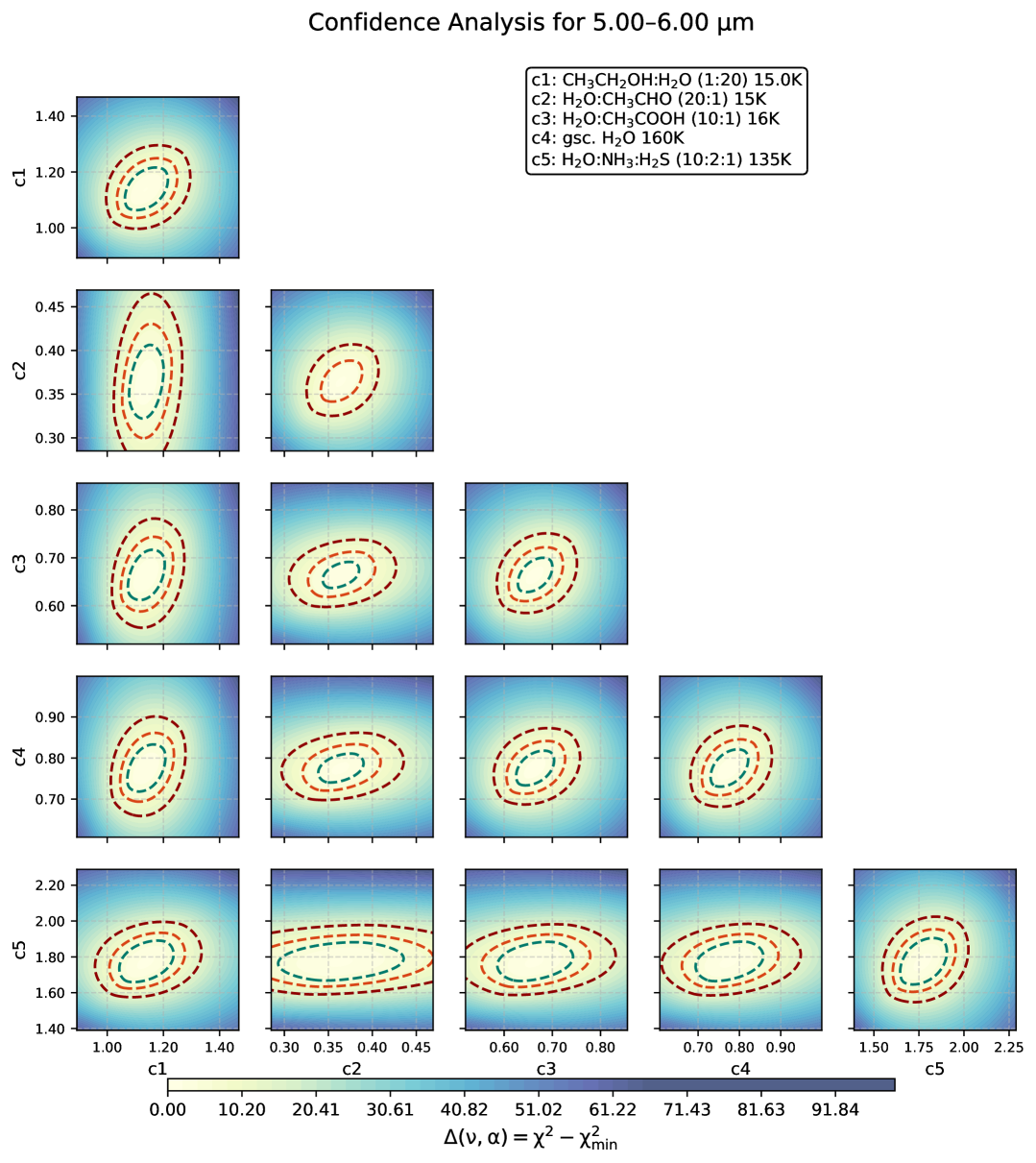
Figure 16: Confidence interval analysis of the components having H₂O bands based on $\chi^{2}$ contributing in 5-6 $\mu$m region. The blue, red and brown dotted lines indicate the 1, 2 and 3 $\sigma$ levels. The coefficients of the remaining components are kept constant while performing this analysis.

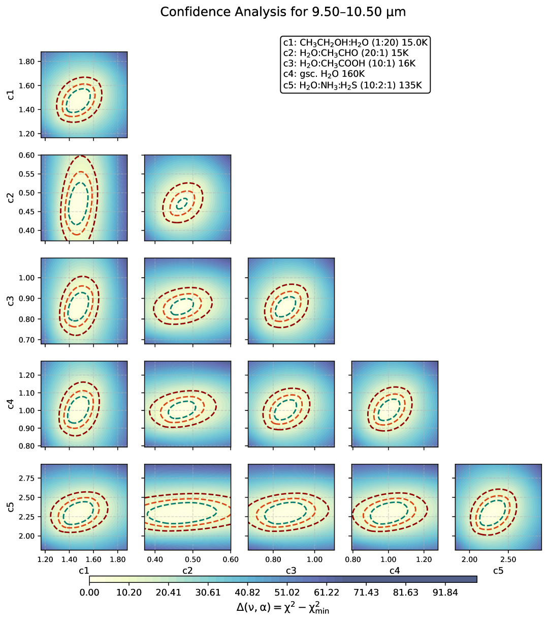
Figure 17: Confidence interval analysis of the components having H₂O bands based on $\chi^{2}$ that are contributing in 9.5-10.5 $\mu$m region. The blue, red and brown dotted lines indicate the 1, 2 and 3 $\sigma$ levels. The coefficients of the remaining components are kept constant while performing this analysis.

In Appendix D, we present the confidence intervals for the model components. Figures 16–18 show the correlations between components containing H₂O bands across three different spectral windows in the 5–20 $\mu$m range. The confidence contours indicate that all components contribute significantly to the fit. Most components show notable mutual correlations, reflecting the spectral overlap inherent to H₂O-rich mixtures. In particular, the H₂O:CH₃COOH and pure H₂O components display strong degeneracy, as evidenced by their elongated elliptical confidence contours, suggesting either spectral overlap or similar contributions within these windows. The H₂O:CH₃CHO component shows a large degree of uncertainty, as reflected in its broad and diffuse contour shapes.

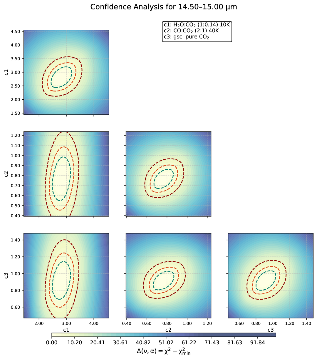
Figure 19: Confidence interval analysis of the CO₂ components based on $\chi^{2}$ in 14.50 - 15 $\mu$m region. The blue, red and brown dotted lines indicate the 1, 2 and 3 $\sigma$ levels. The coefficients of the remaining components are kept constant while performing this analysis.

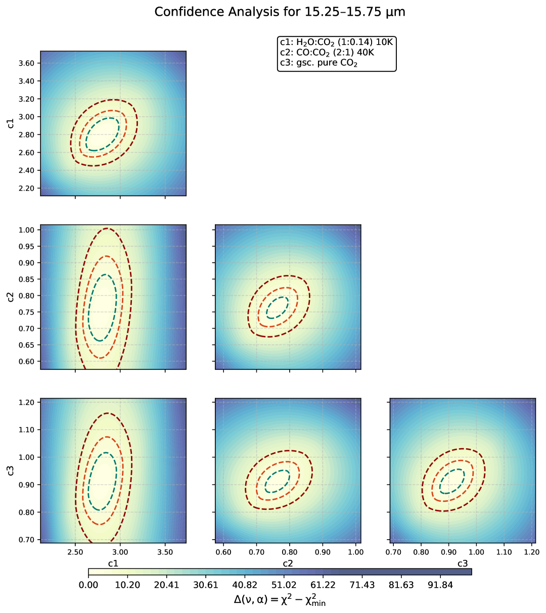
Figure 20: Confidence interval analysis of the CO₂ components based on $\chi^{2}$ in 15.25 - 15.75 $\mu$m region. The blue, red and brown dotted lines indicate the 1, 2 and 3 $\sigma$ levels. The coefficients of the remaining components are kept constant while performing this analysis.

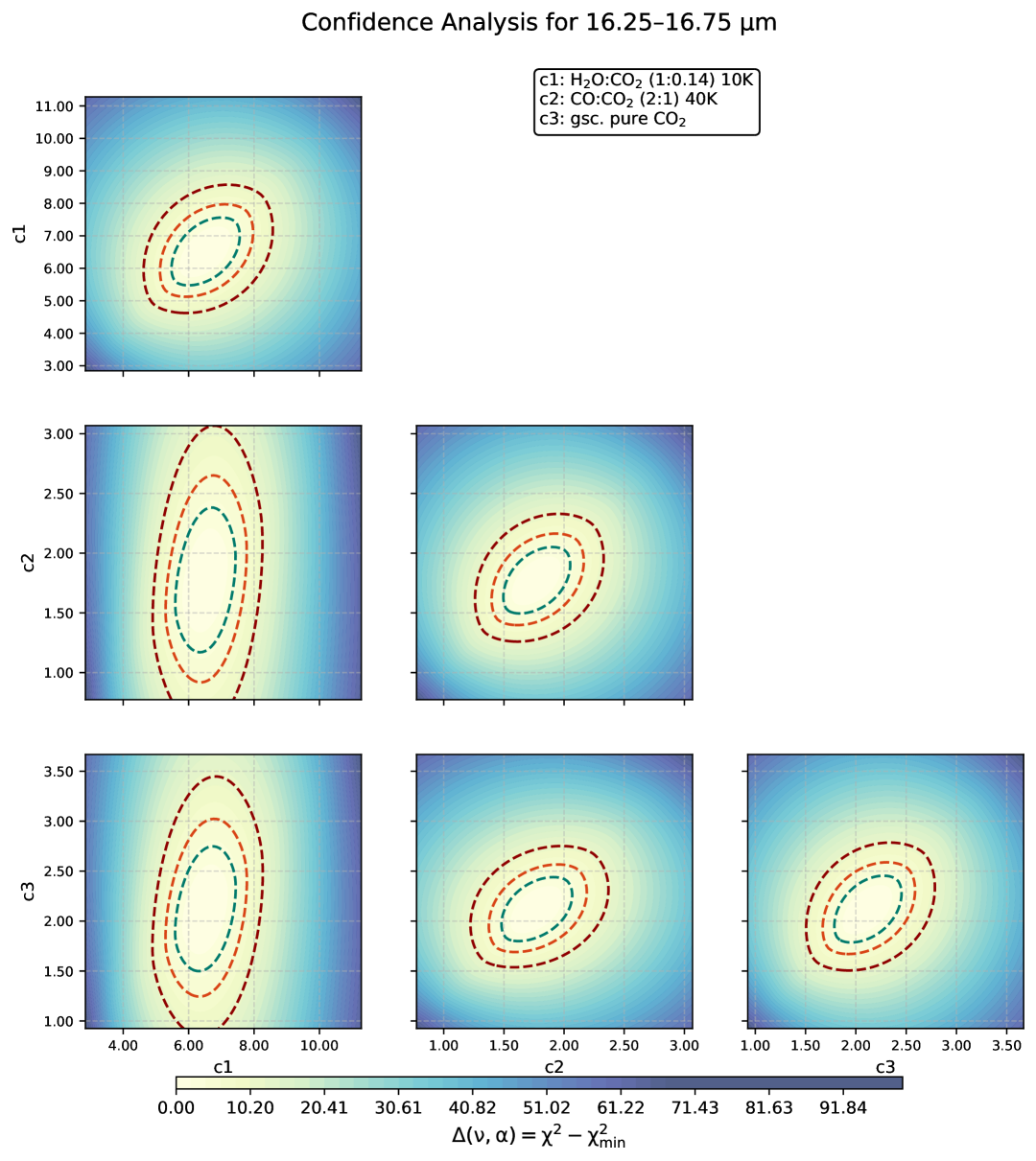
Figure 21: Confidence interval analysis of the CO₂ components based on $\chi^{2}$ in 16.25 - 16.75 $\mu$m region. The blue, red and brown dotted lines indicate the 1, 2 and 3 $\sigma$ levels. The coefficients of the remaining components are kept constant while performing this analysis.

Similarly, the CO₂-bearing components shown in Figures 19–21 show strong mutual correlations, again indicating significant spectral overlap. In particular, the H₂O:CO₂ mixture displays highly elongated confidence contours, pointing to substantial uncertainty in its contribution. The CO:CO₂ mixture and pure CO₂ components also show degeneracy, suggesting considerable spectral overlap, as illustrated in Figure 5. Additionally, the similar widths of their contours imply comparable contributions within the examined windows.

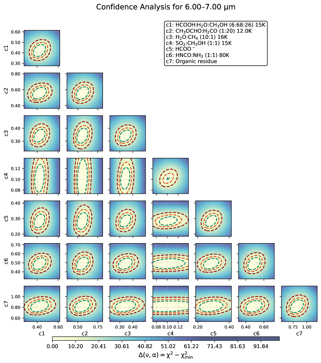
Figure 23: Confidence interval analysis of the components without H₂O and CO₂ bands based on $\chi^{2}$ that are contributing in 14.5-17.5 $\mu$m region. The blue, red and brown dotted lines indicate the 1, 2 and 3 $\sigma$ levels. The coefficients of the remaining components are kept constant while performing this analysis.

The correlation plots for components without H₂O and CO₂ bands are shown in Figures 22–24. These components, which include species such as HCOOH, CH₃OCHO, SO₂, HCOO^-, and complex organic residues, generally show weaker mutual correlations compared to the H₂O- and CO₂-bearing ices, suggesting more confined spectral contributions. Their confidence contours are typically compact and less elongated, indicating lower degeneracy and more distinct contributions in this spectral region. The SO₂ mixture, however, shows considerable uncertainty within its region of influence.

4.5 Column densities and comparison with local fitting results

The ice column densities of different species obtained through global fitting are presented in Table 5. For comparison, we also include column densities derived from local fitting by Rocha et al. (2024), shown in Figure 9. Additionally, abundances relative to H₂O observed toward various sources are presented in Table 5 and are compared in Figures 11 and 10. The column densities derived from global fitting fall within the ranges estimated by local fitting, indicating that both approaches yield consistent results. As shown in Figure 9, most ice species agree within a factor of two between the two methods, with the exception of HCOO^-, whose global fitting estimate is 2.6 times higher than the local fitting result.

This discrepancy in HCOO^- can be interpreted in two ways. On one hand, the global fit includes its strong absorption band at 6.32 $\mu$m, which may support the higher estimate. On the other hand, the value could be overestimated due to fitting uncertainties in the 7.1–7.5 $\mu$m region, where missing components may lead the model to assign extra absorption to HCOO^-. A similar situation is observed for CH₃CH₂OH, which also shows a slightly higher estimate, though still within a factor of two.

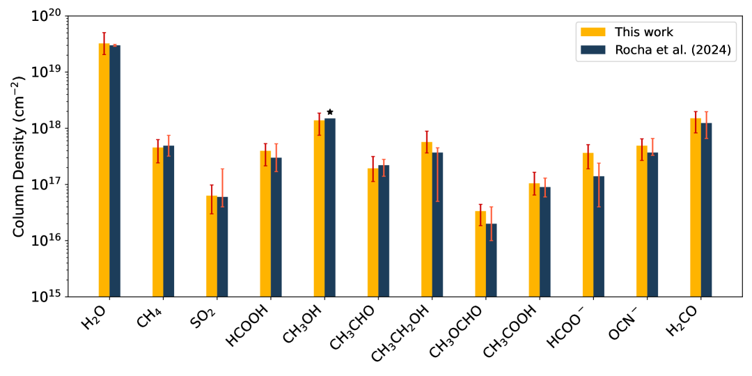
Figure 9: Comparison of ice column densities derived in this work (gold), using global fitting, with those from Rocha et al. (2024) (dark blue) who used local fitting. The x-axis represents different ice species, while the y-axis shows the column densities in cm². Error bars, shown in red, indicate the uncertainties associated with each measurement. For CH₃OH, a factor of 2 or 3 is used in the two fitting methods denoted by star. This agreement highlights the robustness of our global fitting approach using INDRA in capturing the ice inventory consistently with previous studies.

5 Discussions

5.1 Global vs local fitting

From Figure 9, it is evident that global and local fitting yield comparable column densities. In local fitting, the baseline is determined within a narrow spectral window requiring a precise knowledge of the placement of guiding points to anchor the continuum. This method is particularly sensitive to user-defined inputs and can result in the exclusion or misrepresentation of certain components. For example, Rocha et al. (2024) have shown in their Appendix J, how the components such as CH₃CHO and CH₃COOH may be excluded from the fit solely due to the choice of guiding point placement. Since ice spectra contain overlapping absorption bands, determining the continuum placement can be challenging. However, global fitting relies on a single baseline across the entire spectral range and simultaneously considers multiple features of the same ice at different wavelengths. This approach ensures a more self-consistent decomposition of spectral components, reducing uncertainties associated with local continuum selection. For example, in the IRAS 2A optical depth spectrum, the absorption band due to OCN^- at 15.87 $\mu$m overlaps with CO₂ and H₂O, making it almost unrecognizable. In such cases, one might tend to attribute the entire absorption to CO₂ and H₂O ices, potentially overlooking the contribution from OCN^-. However, global fitting accounts for this issue by considering multiple spectral regions where OCN^- shows distinct features, ensuring that its contribution is properly constrained. Also, if the absorption features of different ices are not severely blended with dominant ones, regardless of whether the baseline is determined locally or globally, the overall column densities remain largely unaffected, as they are primarily dictated by the unique absorption strengths and intrinsic band profiles of ices which is the case with CH₄, SO₂ and CH₃OH as shown in the Figure 9. Another drawback of the local fitting approach is that it can disrupt physically meaningful correlations between absorption bands of the same species, potentially leading to inconsistent or unreliable estimates across those bands. For example, HCOO^- shows an intense absorption band at 6.32 $\mu$m, which is nearly twice as strong as its weaker bands at 7.2 and 7.4 $\mu$m. Previous study that employed local fitting within the 6.8–8.6 $\mu$m region was limited to the weaker bands for column density estimation. As a result, these estimates may have been less reliable due to the lower band strengths. In contrast, the global fitting approach adopted in this work leverages the full MIRI range, allowing the inclusion of the stronger 6.32 $\mu$m feature. This leads to a more robust constraint on the HCOO^- abundance, yielding column densities that are nearly twice those derived from local fitting method. However, we caution that this higher value may also be influenced by the spectral gap in the model and observed spectrum due to the absence of certain components in the 7.1–7.5 $\mu$m region, which could lead the model to overfit HCOO^- in the region.

5.2 Treatment of H₂O and CH₃OH bands in some of the ice mixtures

In our spectral fitting analysis, the presence of H₂O and CH₃OH bands in the ice mixtures alongside the features of COMs carries important physical implications. In general, the inclusion of H₂O and CH₃OH absorption features in ice mixtures provides compelling evidence that these species are embedded in H₂O- and CH₃OH-rich matrices, a condition supported by laboratory experiments. Therefore, our general approach has been to retain these bands in ice mixtures wherever possible. However, exceptions were made in cases where the inclusion of dominant H₂O or CH₃OH bands introduced inconsistencies or degeneracy in the spectral fit, primarily due to overlapping contributions from different ice mixtures or uncertain baselines. In three of the COM mixtures, as listed in Table 4, we retain the H₂O bands to reflect the physical co-existence of H₂O and COMs in the ice matrix. The specific cases where dominant band removal was necessary are described below.

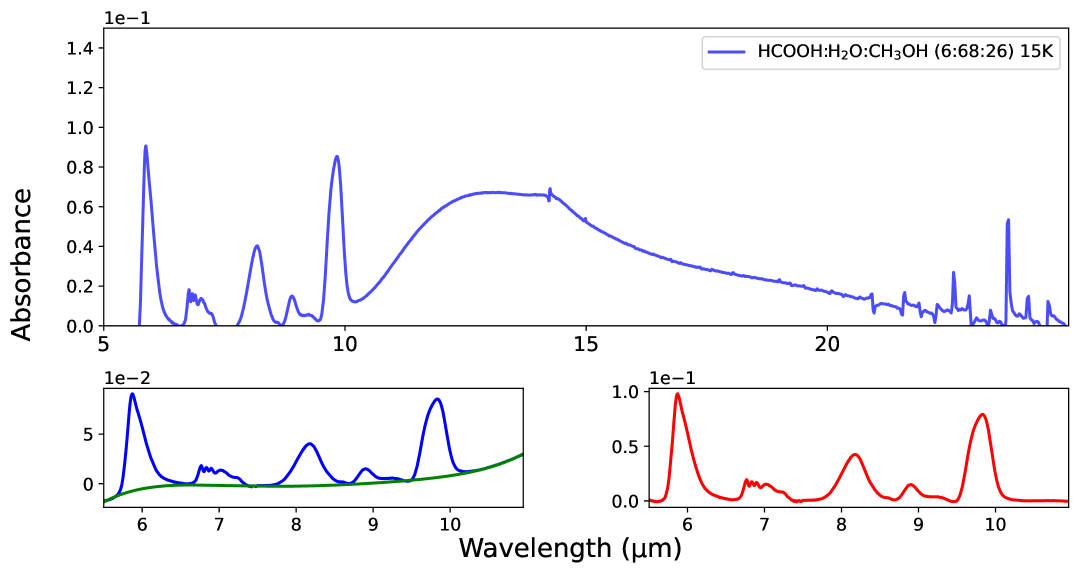
Figure 14: The absorption profile of 15 K ice mixture HCOOH:H₂O:CH₃OH (6:68:26) (Bisschop et al., 2007) is shown in blue in the top panel. Features other than H₂O are shown in the bottom-left panel in blue and the corresponding polynomial baseline in green. The H₂O subtracted spectra is shown in red.

For the HCOOH:H₂O:CH₃OH (6:68:26) 15 K mixture, the global baseline near the 6 $\mu$m H₂O bending mode displayed a non-zero offset and significant relative uncertainty compared to the band peak, as shown in the bottom left panel of the Figure 14. Including the H₂O contribution from this mixture introduced inconsistencies in the modeled spectrum and adversely affected the stability of the fit. Given that H₂O is already well-accounted for by other mixtures in the model, we removed the H₂O bands from this component to ensure stability in the fitting.

For the H₂O:CH₄ (10:1) 16 K mixture, the observed feature near 7.7 $\mu$m in the IRAS 2A optical depth spectrum could be reliably reproduced only when the dominant H₂O bands from this mixture were excluded. Retaining these bands led to overfitting of water features that were already adequately modeled by other components, which degraded the quality of the overall fit in the region. The feature at 7.7 $\mu$m is shaped by the combined contributions of CH₄ (7.67 $\mu$m), SO₂ (7.60 $\mu$m), and the OCN^- ion (7.62 $\mu$m). The improved fit quality around this region can be observed in Figure 4, and the corresponding CH₄ column density estimation compared to the local fitting is shown in Figure 9.

For the SO₂:CH₃OH (1:1) 10 K mixture, isolation of the SO₂ feature was necessary due to the presence of strong CH₃OH absorption band at 9.74 $\mu$m. In the optical depth spectrum of IRAS 2A, this band is already well addressed by CH₃OH band from HCOOH:H₂O:CH₃OH mixture. As a result, including the additional CH₃OH contribution from the SO₂ mixture introduced redundancy and led to the rejection of the component. To address this, we removed the CH₃OH band from this mixture, isolating the SO₂ signatures at 7.60 and 8.68 $\mu$m with the former band being relatively intense one. The column densities of SO₂ and CH₃OH are comparable with the local fitting case and the same is shown in the Figure 9.

5.3 Formation pathway of the detected ices

Using global fitting, we identified multiple ice components contributing to the observed optical depth of IRAS 2A. These include simple molecules like H₂O, CH₄, and NH₃, ions such as OCN^- and NH${}_{4}^{+}$, as well as COMs such as CH₃OH, CH₃OCHO, and HCOOH. Additionally, we noted the possible presence of organic refractory salts. In this section we discuss the formation pathways of these ices.

Simple molecules such as H₂O, CH₄, NH₃, and SO₂ form through a combination of gas-phase and grain-surface reactions in interstellar environments. Water ice primarily forms on dust grains through the hydrogenation of atomic oxygen, while in warmer regions, gas-phase reactions involving oxygen and molecular hydrogen also contribute. Methane is produced via the stepwise hydrogenation of atomic carbon on grain surfaces, a process that occurs efficiently at low temperatures in dense molecular clouds. Similarly, ammonia forms through successive hydrogenation of atomic nitrogen on icy dust grains. Sulfur dioxide, on the other hand, can originate from both gas-phase reactions and surface chemistry. These simple molecules act as fundamental building blocks for more complex ices, undergoing further processing as star and planet formation proceeds.

The presence of ions is conclusive proof that different irradiation processes play a role in the ice chemistry, leading to ionization, dissociation, and recombination reactions within the ice mantles of dust grains. Basically, OCN^- forms efficiently under interstellar conditions through processes involving photolysis or irradiation of CO and NH₃ containing ices (Hudson et al., 2001). It has been observed in interstellar ices (Grim & Greenberg, 1987; Schutte & Khanna, 2003; Van Broekhuizen et al., 2004) and is the primary carrier of the interstellar XCN band. The formate ion is typically formed through acid-base reactions in interstellar ices. Additionally, it can also be produced through surface chemistry involving CO and OH radicals on interstellar grains or via energetic processing (e.g., UV irradiation or cosmic-ray-induced reactions) of ice mixtures containing H₂O, CO, and H₂CO molecules. The formation of NH${}_{4}^{+}$ in interstellar ices primarily occurs through acid-base reactions involving NH₃ and strong acids such as HNCO (grain-surface product). A proton transfer can readily occur in the presence of the strongly nucleophilic NH₃ with even a modest energy input, such as a slight temperature increase or UV radiation (Hasegawa & Herbst, 1993). CH₃CHO and CH₃CH₂OH are chemically linked through sequential hydrogenation in the solid state. The first hydrogenation step converts CH₃CHO into the CH₃CH(OH) radical, which undergoes a second hydrogenation to form CH₃CH₂OH. This process occurs efficiently on icy dust grains under interstellar conditions (Fedoseev et al., 2022). CH₃COOH can form in interstellar ices through oxidation reactions involving CH₃CHO. One proposed pathway involves the reaction of CH₃CHO with OH radicals, leading to CH₃COOH. Additionally, CH₃COOH can form via radical recombination between CH₃O and COOH, both of which are produced through photoprocessing or cosmic-ray-induced chemistry in CO-rich ice mantles. CH₃OCHO forms primarily through surface reactions involving CH₃O and HCO radicals. These radicals originate from CO hydrogenation on icy dust grains, a process that occurs efficiently at low temperatures ($\sim$10–20 K) (e.g., Watanabe & Kouchi (2002); Fuchs et al. (2009)). During this sequence, CO is first hydrogenated to form H₂CO, which can further react with hydrogen to produce CH₃OH. Meanwhile, the CH₃O and HCO radicals, which are intermediates in this process, can recombine to form CH₃OCHO (e.g., Chuang et al. 2016; Garrod et al. 2022; Chen et al. 2023).

The formation of complex organic molecules within icy mantles on dust grains is primarily driven by the condensation of volatile species such as H₂O, CO, CO₂, and NH₃ in dense molecular clouds. Upon exposure to UV radiation from YSOs or external cosmic sources, these ices undergo photodissociation, leading to the generation of reactive radicals. The recombination of these species results in the synthesis of more complex organic molecules, including HMT, ammonium salts of carboxylic acids, amides, esters, and polyoxymethylene (POM)-related species. H₂O ice plays a catalytic role in facilitating these reactions by promoting radical diffusion and stabilizing intermediates. Laboratory experiments confirm that UV photoprocessing of ice mixtures, such as H₂O:CH₃OH:NH₃:CO:CO₂ at temperatures ($\sim$12 K), significantly enhances the formation of refractory organic residues (Muñoz Caro & Schutte, 2003). The transformation of these organics into nonvolatile refractory materials occurs through further energetic processing. Silicate grains, as suggested by He et al. (2024), can incorporate these organics within their interlayer spaces, preserving them as interstellar material evolves into larger interplanetary objects like asteroids and comets.

5.4 Contributions from polar environment

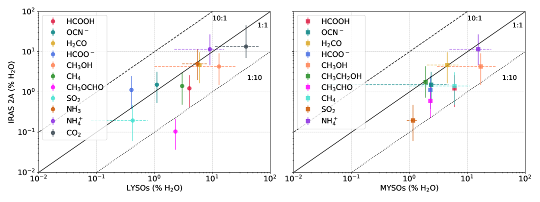
Figure 10: Comparison of ice abundances as a percentage of H₂O of IRAS 2A with those of LYSOs (left panel) and MYSOs (right panel). The solid line represents 1:1 reference, while the dotted and dashed lines indicate abundances that are a reduced and increased by a factor of 10 respectively. Table 5 lists the values used for the comparison of LYSOs and MYSOs with IRAS 2A.)

We observed that most of the organics are associated with water, suggesting a polar environment, which is also consistent with previous work by Rocha et al. (2024). The presence of COMs such as CH₃CHO, CH₃CH₂OH, and CH₃COOH within a H₂O-rich ice matrix indicates that water plays a dominant role in shaping the chemical environment of IRAS 2A. Water, being highly polar, strongly influences the spectral band shapes of these molecules, leading to broader features and peak shifts compared to their absorption in apolar environments. Additionally, laboratory experiments have demonstrated that COMs in polar ice environments exhibit different spectral characteristics compared to those in apolar matrices, further supporting the H₂O-dominated nature of the ice. Observations from the JWST-Ice Age program (McClure et al., 2023) also suggest that CH₃OH, the most abundant COM, coexists with H₂O in cold prestellar clouds, reinforcing the idea that polar interactions dominate the ice chemistry in IRAS 2A. Besides, the experiments by Muñoz Caro & Schutte (2003) suggests the role of H₂O as a catalyst in the formation of large organic molecules at cryogenic temperatures which ultimately leads to the formation of COMs and refractory materials. The significance of a polar environment is also supported by the fact that the observed 7.2 $\mu$m feature in the ISO spectrum toward W 33A was better reproduced by Bisschop et al. (2007) when HCOOH is present in polar environment rather than in CO or CO₂ dominated regions. We have also observed the HCOOH appearing as a tertiary mixture that includes H₂O. This highlights the importance of complex ice-phase interactions through surface reactions involving H, OH, and HCO radicals, primarily in polar environments rich in H₂O and CH₃OH. Altogether, this evidence strongly supports the conclusion that IRAS 2A harbors a polar chemical environment.

5.5 Astrophysical importance of the detected ices

The detection of various ices in IRAS 2A provides crucial insights into the chemical composition and evolution of planetary objects. All the identified ices—including H₂O, CH₄, NH₃, CO, CO₂, and COMs such as CH₃CHO, CH₃CH₂OH, and CH₃COOH—have previously been observed in different astrophysical environments. Figures 10 and 11 show the presence of various ice species and comparison of the ice estimates from this work with those found in LYSOs and MYSOs, as well as in comet 67P. Note the good agreement between the estimated ice column densities and the observations toward LYSOs in the Figure 10. These estimates lie within a factor of 10, indicates that IRAS 2A’s ice composition is broadly comparable to both LYSOs and MYSOs. The left panel of the Figure 10 suggests that IRAS 2A is chemically more similar to LYSOs, supporting its classification as a low-mass protostar in a relatively early evolutionary stage. However, further observational and modeling studies are needed to evaluate the chemical similarity. Figure 11 presents a similar comparison with observations from comet 67P (Rubin et al., 2019). If the ice inventory from earlier phases is inherited by cometary bodies without significant alteration, one would expect a one-to-one correlation, as indicated by the solid line in Figure 11. However, the fractional abundances of most species relative to water are systematically depleted in comet 67P compared to IRAS 2A. This suggests that ices inherited from earlier stages undergo substantial processing before being incorporated into cometary nuclei. Notably, the COMs and their precursors, such as HCOOH and H₂CO, exhibit the strongest depletion, by factors $\gtrsim$10 in comet 67P. In contrast, simpler volatiles like NH₃, SO₂, CH₄, and CO₂ fall within a range of $\sim$ 1–10. This pattern likely reflects the thermal, radiative processing of ices and outgassing of materials during the protostellar-to-disk transition and after, where fragile COMs are easily destroyed or converted, while simpler volatiles can efficiently be re-condensed at low temperatures. These findings support the view that chemical inheritance from the protostellar phase is neither complete nor direct, and that significant chemical evolution occurs between the early envelope stage and the comet formation.

The detection of ions like OCN^-, NH${}_{4}^{+}$, and HCOO^- in IRAS 2A indicates thermal or energetic processing of ices, likely driven by UV photons, cosmic rays, or radiative heating from the protostar. These ions are commonly associated with proton transfer reactions and acid-base chemistry in the ice, suggesting an active chemical evolution. The presence of HCOOH in this ice mixture highlights a chemically rich environment where hydrogen bonding interactions and acid-base equilibria play a crucial role in stabilizing ions and shaping the observed spectral signatures. Additionally, the detection of various COMs and their strong spectral association with H₂O suggest that water ice is a key driver in their formation, either by acting as a chemical catalyst or through hydrogenation pathways that transform simpler molecules into more complex species. The polar nature of the ice environment further influences COM formation by stabilizing reactive intermediates, facilitating radical diffusion, and modifying spectral band shapes, as seen in the JWST observations. Further, the detection of CH₃COOH, HCOOH and CH₃OH highlights their potential role in prebiotic chemistry. This supports the idea that IRAS 2A harbors a chemically dynamic and evolutionarily significant ice reservoir, with potential implications for the prebiotic chemistry inherited by nascent planetary systems.

The inheritance of the refractory organics by carbonaceous chondrites (CR and CM types) further strengthens the connection between interstellar ice chemistry and the complex organic inventory in planetary systems (Danger et al., 2024). Additionally, HMT is known to desorb around 40 K, and its possible presence in protostellar sources, such as IRAS 2A, could be a useful tracer of cold regions where thermal desorption is beginning to release complex organics into the gas phase (Javelle et al., 2024). The detection of HMT in select carbonaceous chondrites (e.g., Murchison, Murray, and Tagish Lake) highlights its potential role in prebiotic chemistry, as its degradation can yield formaldehyde and ammonia—key ingredients for amino acid formation (Oba et al., 2020). However, high-resolution mass spectroscopic data from the Rosetta mission at comet 67P did not confirm the presence of polymers like POMs or HMT, suggesting that thermal processing may have altered these materials in cometary environments (Hänni et al., 2022). The presence or absence of HMT in extraterrestrial materials remains a key question in astrobiology, as its detection could provide significant insight into the molecular pathways that link interstellar ice chemistry with the organic inventory of early planetary bodies. If HMT is widely present in primitive extraterrestrial materials, it could represent a crucial prebiotic reservoir. Furthermore, its possible presence in protostellar sources like IRAS 2A may serve as a valuable probe of early-stage star-forming regions, shedding light on the survival and evolution of prebiotic molecules in cold astrophysical environments.

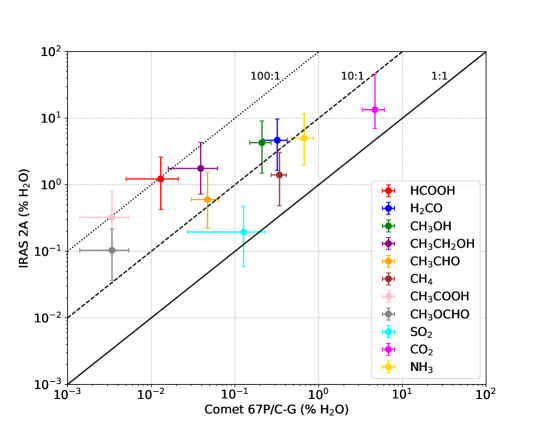
Figure 11: Comparison of ice abundances as a percentage of H₂O of IRAS 2A with those of comet 67P/C-G from Rubin et al. (2019). The solid line represents 1:1 reference, while the dashed and dotted lines indicate cometary abundances that are reduced by factors of 10 and 100, respectively.

6 Conclusion

Based on the spectral fitting of IRAS 2A using a global continuum across the entire JWST MIRI range, along with a comparison of the derived column densities with local fitting values and those observed toward YSOs and comet 67P, the following conclusions can be drawn.

1. The agreement between our derived ice column densities using global fitting and those from previous studies (Rocha et al., 2024) which used local fitting confirms that global fitting can be performed with accuracy comparable to local fitting, demonstrating the robustness of our approach.

2. In complex ice spectra, absorption features of different species often overlap significantly with dominant ice features, making the identification of weaker components challenging, as seen in the case of OCN^- feature blended with H₂O and CO₂ bands. Local fitting, which focuses on isolated spectral regions, may assign the blended features to more dominant species, leading to under-estimation of minor components or over-estimation of major components. In contrast, global fitting leverages multiple spectral regions where each species shows distinct features, ensuring a more accurate and constrained determination of ice composition.

3. The presence of broad absorption features from $\sim$5.5 $\mu$m to $\sim$11 $\mu$m suggests contributions from various functional groups, including carbonyl (C=O), hydroxyl (O–H), amine (N–H), and C–H bending modes, indicating the presence of organic refractory materials. These refractory organics are crucial for understanding irradiation-driven chemical evolution in star- and planet-forming regions, and are likely incorporated into comets, asteroids, and C-type chondrites.

4. The global fitting approach not only improves the accuracy of column density estimates by leveraging the full spectral range and all ice absorption bands but also reveals a rich chemical inventory. This includes simple volatiles such as H₂O, ionic species like NH${}_{4}^{+}$, complex organic molecules (COMs), their precursors, and refractory organic residues—highlighting the chemical complexity of interstellar ices. These findings provide insights into the diverse physical and chemical processes at play in star-forming environments.

5. The spectral association of COMs with H₂O suggests that IRAS 2A hosts a predominantly polar environment. Furthermore, H₂O may actively influence COM chemistry, including the formation of organic refractory materials, by acting as a catalyst.

6. The good correlation of the estimated ice column densities of IRAS 2A with those of both LYSOs and MYSOs within a factor of 10 suggests a chemically linked evolutionary pathway, with IRAS 2A likely representing an early or intermediate stage of a LYSO.

7. The systematic depletion of COMs—and to some extent, simple volatiles—in the cometary ices of 67P relative to H₂O suggests that ices inherited from earlier protostellar phases undergo significant thermal and radiative processing, outgassing, and chemical transformation. This implies that the inheritance of pristine ices is incomplete and that ice compositions are actively reprocessed both prior to and after incorporation into cometary bodies.

Appendix A List of laboratory data

Table 6: Laboratory data used in this work.

Component	Ratio	T (K)	Database	References
pure H2O	-	15-160	LIDA	Öberg et al. (2007)
pure H2O UV irr.	-	10.1	LIDA	Gerakines et al. (1996)
pure H2O UV irr.	-	10.2	LIDA	Gerakines et al. (1996)
H2O:CH4	10:1	15-16	UNIVAP	Rocha et al. (2017)
H2O:CH4	10:0.6	16	UNIVAP	Rocha et al. (2017)
NH3:CH3OH	1:1	15	UNIVAP	Rocha et al. (2020)
H2O:CH3CHO	20:1	15-120	LIDA	Terwisscha van Scheltinga et al. (2018)
pure CH3CHO	-	15-120	LIDA	Terwisscha van Scheltinga et al. (2018)
pure HCOOCH3	-	15	LIDA	Terwisscha van Scheltinga et al. (2021)
CH3CH2OH:H2O	1:20	15-160	LIDA	Terwisscha van Scheltinga et al. (2018)
CH3CN	-	15-150	LIDA	Rachid et al. (2022)
H2O:CO2	1:0.14	10	LIDA	Ehrenfreund et al. (1997)
CO:CO2	2:1	40	LIDA	Schutte et al. (1999)
pure CO2	-	-		Pontoppidan et al. (2008)
H2O:NH3:HCOOH (HCOO-)	100:2.6:2	14	LIDA	Gálvez et al. (2010)
H2O:CH3COOH	10:1	16	NASA	NASA Cosmic Ice Laboratory $\dagger$
H2O:CH3OH:NH3:CO:CO2 (Organic residue)	2:1:1:1:1	12		Muñoz Caro & Schutte (2003)
HCOOH:H2O:CH3OH	6:68:26	15	LIDA	Bisschop et al. (2007)
HNCO:NH3(OCN-)	1:1	80	LIDA	Novozamsky et al. (2001)
pure CH4	-	12.0	OCdb	Hudgins et al. (1993)
CH3COCH3:H2O	1:20	15	LIDA	Rachid et al. (2020)
CH3COCH3:H2CO	1:20	15-150	LIDA	Terwisscha van Scheltinga et al. (2021)
pure SO2	-	10.0	LIDA	Boogert et al. (1997)
SO2:CH3OH	1:1	10	LIDA	Boogert et al. (1997)

Appendix B A note on the band strengths of ices used in this work

The band strengths of molecular ices vary significantly depending on whether they exist in a pure or mixed state. This is due to the intermolecular interactions that alter the vibrational properties of molecules. In pure ices, absorption features arise from the vibrational modes of individual molecules which in fact depend on molecular dipole moment and crystalline structure etc. However, when molecules are present as mixtures, interactions with other species can lead to shifts in band positions, changes in intensity and modifications of band profiles. Consequently, there can either be enhancement or suppression of vibrational modes depending on the nature and strength of that interaction. The latter depends on the physical conditions like temperature as well. For example, Bouwman et al. (2007) found that in H₂O:CO ice mixtures, band intensities vary systematically with concentration, with H₂O features weakening and the free OH stretch strengthening as CO increases. Bouilloud et al. (2015) have derived the correction factors for the band strengths of CO and CO₂ ices based on the works of Gerakines et al. (1995). Such variations in band strengths of ices can impact the ice column density estimations. And, hence it is required to correct the band strengths of ices in order to prevent under or over estimation of abundances.

Table 7: List of vibrational transitions and band strengths of molecules considered in this paper.

Chemical formula	Name	$\lambda\;[\mu\mathrm{m}]$	$\nu\;\mathrm{[cm^{-1}]}$	Identification	$\mathcal{A}\;\mathrm{[cm\;molec^{-1}]}$	References
H2O	Water	13.20	760	libration	$\mathrm{3.2\times 10^{-17}}$	[1][14]
CH4	Methane	7.67	1303	CH4 def.	$\mathrm{8.4\times 10^{-18}}$	[1][2][14]
SO2	Sulfur dioxide	7.60	1320	SO2 stretch.	$\mathrm{3.4\times 10^{-17}}$	[2]
H2CO	Formaldehyde	8.04	1244	CH2 rock.	$\mathrm{1.0\times 10^{-18}}$	[1]
CH3OH	Methanol	9.74	1026	C$-$O stretch.	$\mathrm{1.8\times 10^{-17}}$	[1]
					$\mathrm{1.56\times 10^{-17}}$	[15]
HCOOH	Formic acid	8.22	1216	C$-$O stretch.	$\mathrm{2.9\times 10^{-17}}$	[1]
CH3CHO	Acetaldehyde	7.41	1349	CH3 s-def./CH wag.	$\mathrm{4.1\times 10^{-18}}$	[3][17]
CH3CH2OH	Ethanol	7.23	1383	CH3 s-def.	$\mathrm{2.4\times 10^{-18}}$	[4]
CH3OCHO	Methyl formate	8.25	1211	C$-$O stretch.	$\mathrm{2.52\times 10^{-17}}$	[5]
					$\mathrm{2.28\times 10^{-17}}$	[5]
CH3COOH	Acetic acid	7.82	1278	OH bend.	$\mathrm{4.57\times 10^{-17}}$	[6]
HCOO- (B1)	Formate ion	7.23	1383	C$-$H def.	$\mathrm{8.0\times 10^{-18}}$	[16]
HCOO- (B2)	Formate ion	7.38	1355	C$-$O stretch.	$\mathrm{1.7\times 10^{-17}}$	[16]
OCN-	Cyanate ion	7.62	1312	Comb. (2$\nu_{2}$)	$\mathrm{7.45\times 10^{-18}}$	[6]
NH${}_{4}^{+}$	Ammonium ion	6.85	1428	$\nu_{4}$ (asym. bend.)	$\mathrm{4.4\times 10^{-17}}$	[11]
NH3	Ammonia	9.34	1070	Umbrella mode	$\mathrm{2.1\times 10^{-17}}$	[1]
CO2	Carbon dioxide	15.27	654		1.45$\times\mathrm{1.6\times 10^{-17,a}}$	[12]
HMT	Hexamethylenetetramine	8.1	1234	CN stretch.	$\mathrm{2.6\times 10^{-18}}$	[13]
HMT	Hexamethylenetetramine	9.3	1007	CN stretch.	$\mathrm{5\times 10^{-18}}$	[13]
CA salt	Carboxylic acid salt	6.3	1586		$\mathrm{6\times 10^{-17}}$	[13]
Amide	Amide	5.9	1680		$\mathrm{3.3\times 10^{-17}}$	[13]
Ester	Ester	5.74	1742		$\mathrm{2\times 10^{-17}}$	[13]
POM	polyoxymethylene	9.1	1098		$\mathrm{9.7\times 10^{-18}}$	[13]

Appendix C Baseline corrections

In spectroscopic analysis, local baseline correction is essential for accurately extracting individual absorption features, especially when multiple components contribute to a broad spectral profile. Many ices produce overlapping absorption bands, leading to blended features that obscure individual contributions. In some cases, as in the case of organic molecules, the presence of strong, broad absorption bands from dominant species, say H₂O, can mask weaker features, making their fitting unreliable. By applying a local baseline correction, we can effectively remove underlying continuum variations and overlapping absorptions, ensuring that the extracted spectral features accurately represent the ices of interest. Polynomial baselines are effective in tracing the local continuum and this approach is widely used in many studies. This approach helps in determining ice column densities, and enhances the reliability of spectral fitting.

Appendix D Statistical results

Figure 18: Confidence interval analysis of the components having H₂O bands based on $\chi^{2}$ in 14.75-15.75 $\mu$m region. The blue, red and brown dotted lines indicate the 1, 2 and 3 $\sigma$ levels. The coefficients of the remaining components are kept constant while performing this analysis.

Figure 22: Confidence interval analysis of the components without H₂O and CO₂ bands based on $\chi^{2}$ contributing in 5-6 $\mu$m region. The blue, red and brown dotted lines indicate the 1, 2 and 3 $\sigma$ levels. The coefficients of the remaining components are kept constant while performing this analysis.

Figure 24: Confidence interval analysis of the components without H₂O and CO₂ bands based on $\chi^{2}$ in 5-11 $\mu$m region. The blue, red and brown dotted lines indicate the 1, 2 and 3 $\sigma$ levels. The coefficients of the remaining components are kept constant while performing this analysis.

References

- Argyriou et al. (2023) Argyriou, I., Glasse, A., Law, D. R., et al. 2023, A&A, 675, A111, doi: 10.1051/0004-6361/202346489
- Belloche et al. (2020) Belloche, A., Maury, A. J., Maret, S., et al. 2020, A&A, 635, A198, doi: 10.1051/0004-6361/201937352
- Bisschop et al. (2007) Bisschop, S. E., Fuchs, G. W., Boogert, A. C. A., van Dishoeck, E. F., & Linnartz, H. 2007, A&A, 470, 749, doi: 10.1051/0004-6361:20077464
- Boogert et al. (2022) Boogert, A. C. A., Brewer, K., Brittain, A., & Emerson, K. S. 2022, ApJ, 941, 32, doi: 10.3847/1538-4357/ac9b4a
- Boogert et al. (2015) Boogert, A. C. A., Gerakines, P. A., & Whittet, D. C. B. 2015, ARA&A, 53, 541, doi: 10.1146/annurev-astro-082214-122348
- Boogert et al. (1997) Boogert, A. C. A., Schutte, W. A., Helmich, F. P., Tielens, A. G. G. M., & Wooden, D. H. 1997, A&A, 317, 929
- Boogert et al. (2008) Boogert, A. C. A., Pontoppidan, K. M., Knez, C., et al. 2008, ApJ, 678, 985, doi: 10.1086/533425
- Bottinelli et al. (2007) Bottinelli, S., Ceccarelli, C., Williams, J. P., & Lefloch, B. 2007, A&A, 463, 601, doi: 10.1051/0004-6361:20065139
- Bottinelli et al. (2010) Bottinelli, S., Boogert, A. C. A., Bouwman, J., et al. 2010, ApJ, 718, 1100, doi: 10.1088/0004-637X/718/2/1100
- Boudin et al. (1998) Boudin, N., Schutte, W. A., & Greenberg, J. M. 1998, A&A, 331, 749
- Bouilloud et al. (2015) Bouilloud, M., Fray, N., Bénilan, Y., et al. 2015, MNRAS, 451, 2145, doi: 10.1093/mnras/stv1021
- Bouwman et al. (2007) Bouwman, J., Ludwig, W., Awad, Z., et al. 2007, A&A, 476, 995, doi: 10.1051/0004-6361:20078157
- Brunken et al. (2024) Brunken, N. G. C., van Dishoeck, E. F., Slavicinska, K., et al. 2024, A&A, 692, A163, doi: 10.1051/0004-6361/202451794
- Bushouse et al. (2022) Bushouse, H., Eisenhamer, J., Dencheva, N., et al. 2022, spacetelescope/jwst: JWST 1.6.2, 1.6.2, Zenodo, doi: 10.5281/zenodo.6984366
- Carrasco-Herrera et al. (2024) Carrasco-Herrera, R., Bouquet, A., Danger, G. Â., et al. 2024, in European Planetary Science Congress, EPSC2024–367, doi: 10.5194/epsc2024-367
- Chen et al. (2023) Chen, Y., van Gelder, M. L., Nazari, P., et al. 2023, A&A, 678, A137, doi: 10.1051/0004-6361/202346491
- Chen et al. (2024) Chen, Y., Rocha, W. R. M., van Dishoeck, E. F., et al. 2024, A&A, 690, A205, doi: 10.1051/0004-6361/202450706
- Chu et al. (2020) Chu, L. E. U., Hodapp, K., & Boogert, A. 2020, ApJ, 904, 86, doi: 10.3847/1538-4357/abbfa5
- Chuang et al. (2016) Chuang, K. J., Fedoseev, G., Ioppolo, S., van Dishoeck, E. F., & Linnartz, H. 2016, MNRAS, 455, 1702, doi: 10.1093/mnras/stv2288
- Coutens et al. (2015) Coutens, A., Persson, M. V., Jørgensen, J. K., Wampfler, S. F., & Lykke, J. M. 2015, A&A, 576, A5, doi: 10.1051/0004-6361/201425484
- Danger et al. (2024) Danger, G., Honold, L., Ruf, A., et al. 2024, in European Planetary Science Congress, EPSC2024–596, doi: 10.5194/epsc2024-596
- Dartois et al. (1999) Dartois, E., Schutte, W., Geballe, T. R., et al. 1999, A&A, 342, L32
- Dartois et al. (2003) Dartois, E., Thi, W. F., Geballe, T. R., et al. 2003, A&A, 399, 1009, doi: 10.1051/0004-6361:20021558
- De Simone et al. (2017) De Simone, M., Codella, C., Testi, L., et al. 2017, A&A, 599, A121, doi: 10.1051/0004-6361/201630049
- Dominik et al. (2021) Dominik, C., Min, M., & Tazaki, R. 2021, OpTool: Command-line driven tool for creating complex dust opacities, Astrophysics Source Code Library, record ascl:2104.010. https://ui.adsabs.harvard.edu/abs/2021ascl.soft04010D
- Ehrenfreund et al. (1997) Ehrenfreund, P., Boogert, A. C. A., Gerakines, P. A., Tielens, A. G. G. M., & van Dishoeck, E. F. 1997, A&A, 328, 649
- Fedoseev et al. (2022) Fedoseev, G., Qasim, D., Chuang, K.-J., et al. 2022, ApJ, 924, 110, doi: 10.3847/1538-4357/ac3834
- Fuchs et al. (2009) Fuchs, G. W., Cuppen, H. M., Ioppolo, S., et al. 2009, A&A, 505, 629, doi: 10.1051/0004-6361/200810784
- Gálvez et al. (2010) Gálvez, O., Maté, B., Herrero, V. J., & Escribano, R. 2010, ApJ, 724, 539, doi: 10.1088/0004-637X/724/1/539
- Garrod et al. (2022) Garrod, R. T., Jin, M., Matis, K. A., et al. 2022, ApJS, 259, 1, doi: 10.3847/1538-4365/ac3131
- Gerakines et al. (1996) Gerakines, P., Schutte, W., & Ehrenfreund, P. 1996, Astronomy and Astrophysics, v. 312, p. 289-305, 312, 289
- Gerakines et al. (1995) Gerakines, P. A., Schutte, W. A., Greenberg, J. M., & van Dishoeck, E. F. 1995, A&A, 296, 810, doi: 10.48550/arXiv.astro-ph/9409076
- Gibb & Whittet (2002) Gibb, E. L., & Whittet, D. C. B. 2002, ApJ, 566, L113, doi: 10.1086/339633
- Gibb et al. (2004) Gibb, E. L., Whittet, D. C. B., Boogert, A. C. A., & Tielens, A. G. G. M. 2004, ApJS, 151, 35, doi: 10.1086/381182
- Gieser et al. (2021) Gieser, C., Beuther, H., Semenov, D., et al. 2021, A&A, 648, A66, doi: 10.1051/0004-6361/202039670
- Greenfield & Miller (2016) Greenfield, P., & Miller, T. 2016, Astronomy and Computing, 16, 41, doi: 10.1016/j.ascom.2016.04.001
- Grim et al. (1991) Grim, R. J. A., Baas, F., Geballe, T. R., Greenberg, J. M., & Schutte, W. A. 1991, A&A, 243, 473
- Grim & Greenberg (1987) Grim, R. J. A., & Greenberg, J. M. 1987, ApJ, 321, L91, doi: 10.1086/185012
- Hänni et al. (2022) Hänni, N., Altwegg, K., Combi, M., et al. 2022, Nature Communications, 13, 3639, doi: 10.1038/s41467-022-31346-9
- Hasegawa & Herbst (1993) Hasegawa, T. I., & Herbst, E. 1993, MNRAS, 261, 83, doi: 10.1093/mnras/261.1.83
- He et al. (2024) He, Y. Y., Bernard, S., Lecasble, M., et al. 2024, Geochim. Cosmochim. Acta, 387, 98, doi: 10.1016/j.gca.2024.09.035
- Hudgins et al. (1993) Hudgins, D. M., Sandford, S. A., Allamandola, L. J., & Tielens, A. G. G. M. 1993, ApJS, 86, 713, doi: 10.1086/191796
- Hudson & Ferrante (2020) Hudson, R. L., & Ferrante, R. F. 2020, MNRAS, 492, 283, doi: 10.1093/mnras/stz3323
- Hudson et al. (2005) Hudson, R. L., Moore, M. H., & Cook, A. M. 2005, Advances in Space Research, 36, 184, doi: 10.1016/j.asr.2005.01.017
- Hudson et al. (2001) Hudson, R. L., Moore, M. H., & Gerakines, P. A. 2001, ApJ, 550, 1140, doi: 10.1086/319799
- Ishii et al. (2002) Ishii, M., Nagata, T., Chrysostomou, A., & Hough, J. H. 2002, AJ, 124, 2790, doi: 10.1086/344070
- Javelle et al. (2024) Javelle, T., Ruf, A., Bouquet, A., Schmitt-Kopplin, P., & Danger, G. 2024, MNRAS, 534, 2305, doi: 10.1093/mnras/stae2186
- Jørgensen et al. (2020) Jørgensen, J. K., Belloche, A., & Garrod, R. T. 2020, ARA&A, 58, 727, doi: 10.1146/annurev-astro-032620-021927
- Labiano et al. (2021) Labiano, A., Argyriou, I., Álvarez-Márquez, J., et al. 2021, A&A, 656, A57, doi: 10.1051/0004-6361/202140614
- Looney et al. (2000) Looney, L. W., Mundy, L. G., & Welch, W. J. 2000, ApJ, 529, 477, doi: 10.1086/308239
- Luna et al. (2018) Luna, R., Molpeceres, G., Ortigoso, J., et al. 2018, A&A, 617, A116, doi: 10.1051/0004-6361/201833463
- Luo et al. (2005) Luo, J., Ying, K., & Bai, J. 2005, Signal Processing, 85, 1429, doi: 10.1016/j.sigpro.2005.02.002
- Manigand et al. (2020) Manigand, S., Jørgensen, J. K., Calcutt, H., et al. 2020, A&A, 635, A48, doi: 10.1051/0004-6361/201936299
- Mathurin et al. (2024) Mathurin, J., Bejach, L., Dartois, E., et al. 2024, A&A, 684, A198, doi: 10.1051/0004-6361/202347435
- McClure et al. (2023) McClure, M. K., Rocha, W. R. M., Pontoppidan, K. M., et al. 2023, Nature Astronomy, 7, 431, doi: 10.1038/s41550-022-01875-w
- Muñoz Caro & Schutte (2003) Muñoz Caro, G. M., & Schutte, W. A. 2003, A&A, 412, 121, doi: 10.1051/0004-6361:20031408
- Nazari et al. (2021) Nazari, P., van Gelder, M. L., van Dishoeck, E. F., et al. 2021, A&A, 650, A150, doi: 10.1051/0004-6361/202039996
- Novozamsky et al. (2001) Novozamsky, J. H., Schutte, W. A., & Keane, J. V. 2001, A&A, 379, 588, doi: 10.1051/0004-6361:20011332
- Oba et al. (2020) Oba, Y., Takano, Y., Naraoka, H., et al. 2020, Nature Communications, 11, 6243, doi: 10.1038/s41467-020-20038-x
- Öberg & Bergin (2021) Öberg, K. I., & Bergin, E. A. 2021, Phys. Rep., 893, 1, doi: 10.1016/j.physrep.2020.09.004
- Öberg et al. (2008) Öberg, K. I., Boogert, A. C. A., Pontoppidan, K. M., et al. 2008, ApJ, 678, 1032, doi: 10.1086/533432
- Öberg et al. (2011) —. 2011, ApJ, 740, 109, doi: 10.1088/0004-637X/740/2/109
- Öberg et al. (2007) Öberg, K. I., Fraser, H. J., Boogert, A. C. A., et al. 2007, A&A, 462, 1187, doi: 10.1051/0004-6361:20065881
- Pontoppidan et al. (2005) Pontoppidan, K. M., Dullemond, C. P., van Dishoeck, E. F., et al. 2005, ApJ, 622, 463, doi: 10.1086/427688
- Pontoppidan et al. (2004) Pontoppidan, K. M., van Dishoeck, E. F., & Dartois, E. 2004, A&A, 426, 925, doi: 10.1051/0004-6361:20041276
- Pontoppidan et al. (2008) Pontoppidan, K. M., Boogert, A. C. A., Fraser, H. J., et al. 2008, ApJ, 678, 1005, doi: 10.1086/533431
- Rachid et al. (2021) Rachid, M. G., Brunken, N., de Boe, D., et al. 2021, A&A, 653, A116, doi: 10.1051/0004-6361/202140782
- Rachid et al. (2022) Rachid, M. G., Rocha, W. R. M., & Linnartz, H. 2022, A&A, 665, A89, doi: 10.1051/0004-6361/202243417
- Rachid et al. (2020) Rachid, M. G., Terwisscha van Scheltinga, J., Koletzki, D., & Linnartz, H. 2020, A&A, 639, A4, doi: 10.1051/0004-6361/202037497
- Reipurth et al. (2002) Reipurth, B., Rodríguez, L. F., Anglada, G., & Bally, J. 2002, AJ, 124, 1045, doi: 10.1086/341172
- Rieke et al. (2015) Rieke, G. H., Wright, G. S., Böker, T., et al. 2015, PASP, 127, 584, doi: 10.1086/682252
- Rocha et al. (2021) Rocha, W. R. M., Perotti, G., Kristensen, L. E., & Jørgensen, J. K. 2021, A&A, 654, A158, doi: 10.1051/0004-6361/202039360
- Rocha et al. (2017) Rocha, W. R. M., Pilling, S., de Barros, A. L. F., et al. 2017, MNRAS, 464, 754, doi: 10.1093/mnras/stw2398
- Rocha et al. (2020) Rocha, W. R. M., Pilling, S., Domaracka, A., Rothard, H., & Boduch, P. 2020, Spectrochimica Acta Part A: Molecular Spectroscopy, 228, 117826, doi: 10.1016/j.saa.2019.117826
- Rocha et al. (2024) Rocha, W. R. M., van Dishoeck, E. F., Ressler, M. E., et al. 2024, A&A, 683, A124, doi: 10.1051/0004-6361/202348427
- Rocha et al. (2025) Rocha, W. R. M., McClure, M. K., Sturm, J. A., et al. 2025, A&A, 693, A288, doi: 10.1051/0004-6361/202451505
- Rubin et al. (2019) Rubin, M., Altwegg, K., Balsiger, H., et al. 2019, MNRAS, 489, 594, doi: 10.1093/mnras/stz2086
- Sandell et al. (1994) Sandell, G., Knee, L. B. G., Aspin, C., Robson, I. E., & Russell, A. P. G. 1994, A&A, 285, L1
- Savitzky & Golay (1964) Savitzky, A., & Golay, M. J. E. 1964, Analytical Chemistry, 36, 1627, doi: 10.1021/ac60214a047
- Schutte & Khanna (2003) Schutte, W. A., & Khanna, R. K. 2003, A&A, 398, 1049, doi: 10.1051/0004-6361:20021705
- Schutte et al. (1999) Schutte, W. A., Boogert, A. C. A., Tielens, A. G. G. M., et al. 1999, A&A, 343, 966
- Shimonishi et al. (2010) Shimonishi, T., Onaka, T., Kato, D., et al. 2010, A&A, 514, A12, doi: 10.1051/0004-6361/200913815
- Skinner et al. (1992) Skinner, C. J., Tielens, A. G. G. M., Barlow, M. J., & Justtanont, K. 1992, ApJ, 399, L79, doi: 10.1086/186611
- Slavicinska et al. (2023) Slavicinska, K., Rachid, M. G., Rocha, W. R. M., et al. 2023, A&A, 677, A13, doi: 10.1051/0004-6361/202346996
- Slavicinska et al. (2025) Slavicinska, K., Boogert, A. C. A., Tychoniec, Ł., et al. 2025, A&A, 693, A146, doi: 10.1051/0004-6361/202451383
- Taquet et al. (2015) Taquet, V., López-Sepulcre, A., Ceccarelli, C., et al. 2015, ApJ, 804, 81, doi: 10.1088/0004-637X/804/2/81
- Terwisscha van Scheltinga et al. (2018) Terwisscha van Scheltinga, J., Ligterink, N. F. W., Boogert, A. C. A., van Dishoeck, E. F., & Linnartz, H. 2018, A&A, 611, A35, doi: 10.1051/0004-6361/201731998
- Terwisscha van Scheltinga et al. (2021) Terwisscha van Scheltinga, J., Marcandalli, G., McClure, M. K., Hogerheijde, M. R., & Linnartz, H. 2021, arXiv e-prints, arXiv:2105.02226. https://arxiv.org/abs/2105.02226
- Thi et al. (2006) Thi, W. F., van Dishoeck, E. F., Dartois, E., et al. 2006, A&A, 449, 251, doi: 10.1051/0004-6361:20052931
- Tobin et al. (2015) Tobin, J. J., Dunham, M. M., Looney, L. W., et al. 2015, ApJ, 798, 61, doi: 10.1088/0004-637X/798/1/61
- Urso et al. (2024) Urso, R. G., Alemanno, G., Baratta, G. A., et al. 2024, in European Planetary Science Congress, EPSC2024–800, doi: 10.5194/epsc2024-800
- Van Broekhuizen et al. (2004) Van Broekhuizen, F. A., Keane, J. V., & Schutte, W. A. 2004, 415, 425, doi: 10.1051/0004-6361:20034161
- van Broekhuizen et al. (2005) van Broekhuizen, F. A., Pontoppidan, K. M., Fraser, H. J., & van Dishoeck, E. F. 2005, A&A, 441, 249, doi: 10.1051/0004-6361:20041711
- van Gelder et al. (2020) van Gelder, M. L., Tabone, B., Tychoniec, Ł., et al. 2020, A&A, 639, A87, doi: 10.1051/0004-6361/202037758
- van Gelder et al. (2024) van Gelder, M. L., Ressler, M. E., van Dishoeck, E. F., et al. 2024, A&A, 682, A78, doi: 10.1051/0004-6361/202348118
- Wagner & Hornig (1950) Wagner, E. L., & Hornig, D. F. 1950, 18, 296, doi: 10.1063/1.1747622
- Watanabe & Kouchi (2002) Watanabe, N., & Kouchi, A. 2002, ApJ, 571, L173, doi: 10.1086/341412
- Weingartner & Draine (2001) Weingartner, J. C., & Draine, B. T. 2001, ApJ, 548, 296, doi: 10.1086/318651
- Wells et al. (2015) Wells, M., Pel, J. W., Glasse, A., et al. 2015, PASP, 127, 646, doi: 10.1086/682281
- Woitke et al. (2016) Woitke, P., Min, M., Pinte, C., et al. 2016, A&A, 586, A103, doi: 10.1051/0004-6361/201526538
- Wright et al. (2015) Wright, G. S., Wright, D., Goodson, G. B., et al. 2015, PASP, 127, 595, doi: 10.1086/682253
- Wright et al. (2023) Wright, G. S., Rieke, G. H., Glasse, A., et al. 2023, PASP, 135, 048003, doi: 10.1088/1538-3873/acbe66
- Yang et al. (2022) Yang, Y.-L., Green, J. D., Pontoppidan, K. M., et al. 2022, ApJ, 941, L13, doi: 10.3847/2041-8213/aca289