Non-linear in-plane spin current in spin-orbit coupled 2D hole gases

Abstract

The non-linear transport of charge and spin due to the emergence of band geometric effects has garnered much interest in recent years. In this work, we show that a linear in-plane spin current vanishes, whereas a non-linear (second-order) in-plane spin current exists for a generic two-dimensional system having time-reversal symmetry. The intrinsic second-order spin current originates from the spin Berry curvature polarizability. The formulation when applied to 2D hole gases with the $k^{3}$ Rashba spin-orbit interaction reveals the existence of both transverse and longitudinal second-order in-plane spin currents normal to the spin orientation. Further, the effects of band anisotropy due to additional Dresselhaus spin-orbit interaction or an electromagnetic radiation are explored, which allows the generation of additional in-plane spin currents parallel to the spin orientation in the same system. The time-reversal symmetry also prevents any out-of-plane spin current in the second-order. The generation and control over the multiple in-plane spin currents may have important applications in spintronic devices.

I Introduction

The spin Hall effect (SHE) belongs to the family of anomalous Hall effects, where a transport transverse to an applied electric field is observed in the absence of an external magnetic field. Spin Hall effect involves the transport of spin instead of charge, such that carriers in different spin states (up and down) are accumulated on the opposite edges of the sample. This was first studied by D’yakonov and Perel [1] and later by Hirsch [2]. The key difference in the mechanisms of SHE and anomalous charge Hall transport lies in the breaking of time-reversal symmetry ($\mathcal{T}$). The latter is mainly observed in magnetic materials where $\mathcal{T}$ is broken by the spontaneous magnetization, whereas SHE does not require $\mathcal{T}$ to break. The central role in SHE is played by spin-orbit coupling (SOC), which arises due to a broken structural inversion symmetry ($\mathcal{P}$) of the material. There are namely the Rashba spin-orbit coupling [3] and the Dresselhaus spin-orbit coupling [4]. This article, like most others [5],[6] will involve both of these interactions in the system.

Based on the mechanism, SHE can be classified as intrinsic [7] and extrinsic [8]. The latter occurs due to spin-dependent scattering processes from impurities like skew-scattering [9, 10] and side-jumping [11]. The intrinsic SHE, on the other hand has its origin in the geometry of the quantum states of the charge carriers, manifested in the Berry curvature. Although the theory of anomalous Hall effect was given by Karplus and Luttinger back in 1954 [12], it was only after the discovery of Berry phase in 1984 [13] when the role of quantum geometry in Hall transport phenomena began to be explored [14].

Understanding the role of quantum geometry in SHE is of prime importance in current times when non-linear anomalous Hall effect has already been attributed to the quantum metric [15] and the Berry curvature dipole [16, 17]. Berry connection polarizability (BCP), which is the corrected Berry connection due to an applied electric field is known to give rise to non-linear intrinsic Hall responses in $\mathcal{PT}$ symmetry-broken anti-ferromagnets [18, 19].

Attempts to explain SHE in terms of quantum geometrical elements are also underway. In Ref. [20], it is shown that the intrinsic spin Hall current can be derived from the anomalous velocity of electrons in $\mathcal{T}$-broken Rashba spin-orbit coupled systems, thus emphasizing the role of the Berry curvature. Further, instead of the conventional Kubo formula used in [7] and elsewhere to calculate the spin current, Zhang et. al, [21] shows that a spin Berry curvature (SBC) can be derived from a simple perturbation theory to calculate the spin Hall conductivity. Coming to non-linear SHE, apart from the Drude effect [22, 17] and the spin Berry curvature dipole [23], which lead to extrinsic SHE, Zhang et.al [21] using their perturbative approach, have derived an intrinsic second-order spin current from the spin Berry curvature polarizability (SBCP).

In this paper, we apply the perturbative formalism developed in [21] to two-dimensional hole gases (2DHG) formed at the hetero-junctions of III-V p-doped semiconductors to calculate the linear and second-order spin conductivity. Previously, studies on linear SHE in hole gases were carried out by [24, 25, 26, 27, 28, 29]. The calculations are done in the $\mathcal{T}$ symmetric heavy hole band of the spectrum, discussed in detail by Murakami et.al, [24] and Schliemann and Loss [26]. It is known that the linear spin conductivity in hole gases is contributed mainly by the intrinsic mechanism since, the vertex corrections due to impurity scattering vanish for such systems [25, 30]. We particularly emphasize the spin orientations in the SBC and SBCP tensor components and note that they are out-of-plane and in-plane in the first-order and second-order spin currents, respectively. This is shown to be true for any two-level system where $\mathcal{T}$ is preserved [31]. Further, the role of anisotropy in the dispersion relations of these systems is also discussed. Apart from the Dresselhaus effect, the role of electromagnetic radiation in introducing anisotropy is also explored.

This paper is arranged in the following way: section(II) introduces the formalism of second-order spin current and applies it to a general two-level $\mathcal{T}$ symmetric system. Section(III) presents the results obtained for a 2DHG with the Rashba and Dresselhaus SOC. Section(IV) discusses the effect of radiation on the first and second-order spin conductivity of a Rashba spin-orbit coupled hole gas. Finally, we conclude with discussions and potential applications of our results in the field of spintronics.

II The formalism

II.1 Second-order spin current using perturbation theory

In this section, we discuss the general formalism of linear and nonlinear spin currents resulting from SBC and SBCP, in $\mathcal{T}$ preserved systems. This formalism is based on the Boltzmann transport equation within relaxation time approximation and the first-order correction to the Bloch states due to external electric field.

The conventional spin current operator is defined as $\hat{j}^{l}_{i}=\hbar(\sigma_{l}\hat{v}_{i}+\hat{v}_{i}\sigma_{l})/4$, where $\hat{v}_{i}$ is the band velocity operator and $\sigma_{l}$ is the usual Pauli spin operator. The expectation value of the spin current operator in the Bloch states $|n\rangle$ of the $n$-th band is given by $j^{l}_{i,n}=\langle n|\hat{j}^{l}_{i,n}|n\rangle$. The total spin current from $n$ bands in two-dimensional systems can be evaluated as

$$J^{l}_{i}=\sum_{n}\int_{k}[d{\bf k}]~j^{l}_{i,n}f_{n}({\bf k}),$$ (1)

where $[d{\bf k}]=(d^{2}k)/(2\pi)^{2}$, the subscript $i$ ($i=x,y$) and the superscript $l$ ($l=x,y,z$) denote the directions of the spin current and spin polarization of the charge carrier, respectively. Also, $f_{n}({\bf k})$ is the non-equilibrium Fermi-Dirac occupation number for the $n$-th energy band.

An in-plane homogeneous electric field ${\bf E}=E_{x}\hat{\bf x}+E_{y}\hat{\bf y}$ is applied to the system, due to which the perturbation to the Hamiltonian is $H^{\prime}=q{\bf E}\cdot{\bf r}$, where $q$ is the charge of a carrier. Within the first-order perturbation theory, the modified state is given by $|\tilde{n}\rangle=|n\rangle+|\tilde{n}\rangle$, where

$$|\tilde{n}\rangle=\sum_{m\neq n}\frac{-q{\bf E}\cdot{\bf A}_{mn}}{\varepsilon_{m}^{(0)}({\bf k})-\varepsilon_{n}^{(0)}({\bf k})}|m\rangle$$ (2)

with ${\bf A}_{mn}=\langle m|i{\bm{\nabla}}_{\bf k}|n\rangle$ is the interband Berry connection and $\varepsilon_{n}^{(0)}$ are the unperturbed energy eigenvalues. The first-order correction to the Berry curvature ${\bm{\Omega}}_{n}$ can be obtained from ${\bm{\Omega}}_{n}^{(1)}={\bm{\nabla}}_{\bf k}\times{\bf A}_{n}^{(1)}$, where ${\bf A}_{n}^{(1)}=\langle\tilde{n}|i{\bm{\nabla}}_{\bf k}|n\rangle+c.c.$ is the first-order correction to the Berry connection. It can be re-written in Cartesian coordinates as $A_{ni}^{(1)}=G_{ij}^{n}E_{j}$, where

$$G_{ij,n}=-2q\text{Re}\sum_{m\neq n}\frac{A_{nm,i}A_{mn,j}}{\varepsilon_{m}^{(0)}-\epsilon_{n}^{(0)}}$$ (3)

is the band geometric quantity known as Berry connection polarizability. The electric field induced modified spin current (upto quadratic in ${\bf E}$) is $\tilde{j}^{l}_{i,n}=\langle\tilde{n}|\hat{j}^{l}_{i,n}|\tilde{n}\rangle$. After simplification, one can obtain

$$\tilde{j}^{l}_{i,n}=j^{l}_{i,n}-e\Omega^{l}_{ij,n}E_{j}+e^{2}\Pi^{l}_{ijk,n}E_{j}E_{k},$$ (4)

where

$$\Omega^{l}_{ij,n}=\hbar\sum_{m\neq n}2\>\text{Im}{\Big{[}\frac{\langle n|\hat{j}^{l}_{i}|m\rangle\langle m|\hat{v}_{j}|n\rangle}{(\varepsilon^{(0)}_{n}-\varepsilon^{(0)}_{m})^{2}}\Big{]}},$$ (5)

is called spin Berry curvature and

$$\Pi^{l}_{ijk,n}=\hbar^{2}\sum_{m\neq n,q\neq n}\frac{\langle q|\hat{j}^{l}_{i}|m\rangle\langle n|\hat{v}_{j}|q\rangle\langle m|\hat{v}_{k}|n\rangle}{(\varepsilon^{(0)}_{n}-\varepsilon^{(0)}_{q})^{2}(\varepsilon^{(0)}_{n}-\varepsilon^{(0)}_{m})^{2}},$$ (6)

is called spin Berry curvature polarizability.

Within the relaxation time approximation [32], the non-equilibrium Fermi-Dirac occupation number $f_{n}({\bf k})$ can be obtained by solving the Boltzmann transport equation

$$\frac{q}{\hbar}{\bf E}\cdot{\bm{\nabla}}_{\bf k}f_{n}({\bf k})=-\frac{[f_{n}({\bf k})-f_{n}^{(0)}({\bf k})]}{\tau},$$ (7)

where $\tau$ is the relaxation time of the charge carriers and $f_{n}^{(0)}({\bf k})=1/(e^{[\epsilon_{n}({\bf k})-\mu]/(k_{B}T)}+1)$ is the occupation number in absence of the electric field. The iterative solution for $f_{n}({\bf k})$ can be written as

$$f_{n}({\bf k})=\sum_{p}\left(\frac{e\tau}{\hbar}\right)^{p}\frac{\partial^{p}f_{n}^{(0)}}{\partial k^{p}_{i}}E^{p}_{i},$$ (8)

where $p=1,2,3...$.

The total modified spin current we get

$$\tilde{J}^{l}_{i}=\sum_{n}\sum_{p}\int_{k}[d{\bf k}]\tilde{j}^{l}_{i,n}\left(\frac{e\tau}{\hbar}\right)^{p}\frac{\partial^{p}f_{n}^{(0)}}{\partial k^{p}_{i}}E^{p}_{i}.$$ (9)

Now putting the expression for $\tilde{j}^{l}_{i,n}$ from Eq. (4), we get

$$\tilde{J}^{l}_{i}=\sigma^{l}_{i}+\chi^{l}_{ij}E_{j}+\Gamma^{l}_{ijk}E_{j}E_{k}+...\>,$$ (10)

where the spin transport coefficients are given by

$$\sigma^{l}_{i}=\sum_{n}\int_{k}[d{\bf k}]j^{l}_{i,n}f_{n}^{(0)},$$ (11)

$$\chi^{l}_{ij}=e\sum_{n}\int_{k}[d{\bf k}]\Big{(}j^{l}_{i,n}\frac{\tau}{\hbar}\frac{\partial f_{n}^{(0)}}{\partial k_{j}}-\Omega^{l}_{ij,n}f_{n}^{(0)}\Big{)},$$ (12)

$$\Gamma^{l}_{ij\kappa}=e^{2}\sum_{n}\int_{k}[d{\bf k}]\Big{(}j^{l}_{i,n}\frac{\tau^{2}}{\hbar^{2}}\frac{\partial^{2}}{\partial k_{j}\partial{k}_{\kappa}}-\frac{\tau}{\hbar}\Omega^{l}_{ij,n}\frac{\partial}{\partial k_{\kappa}}+\Pi^{l}_{ij\kappa,n}\Big{)}f_{n}^{(0)}$$ (13)

These are the expressions of the zeroth-order, first-order, and second-order spin conductivities, respectively. The $\tau$-dependent and $\tau$-independent terms in the non-linear spin conductivities are the extrinsic and intrinsic contributions, respectively. For $\mathcal{T}$-symmetric systems, the term involving odd power of $\tau$ will vanish exactly, whereas the even power of $\tau$ will have finite contribution [21]. Therefore, the $\tau$-linear term in Eqs. (12) and (13) will be absent for $\mathcal{T}$-symmetric systems, where the structural inversion ($\mathcal{P}$) symmetry is broken. The spin currents computed in the following sections will have components both transverse and longitudinal to the applied electric field. The name spin ’Hall’ current/conductivity is reserved only for the transverse components.

II.2 Results for a generic 2-level $\mathcal{T}$-symmetric system

Let us consider a general time-reversal symmetric two-level system whose Hamiltonian is given by

$$H=\frac{\hbar^{2}k^{2}}{2m}I+{\bf d}({\bf k})\cdot{\bm{\sigma}},$$ (14)

where $I$ is the $2\times 2$ identity matrix and ${\bf d}=\big{(}d_{x}({\bf k}),\;d_{y}({\bf k})\big{)}$ and ${\bm{\sigma}}=(\sigma_{x},\sigma_{y})$. So the spin dependent part of the Hamiltonian is given by,

$$H_{s}={\bf d}\cdot{\bm{\sigma}}=d_{x}\sigma_{x}+d_{y}\sigma_{y}.$$ (15)

Here the Pauli matrices represent real spin of the charge carrier and since there is no term containing $\sigma_{z}$ so that $\mathcal{T}$ is preserved. On diagonalization the eigenvalues and eigen states are obtained as functions of ${\bf k}$:

$$\varepsilon_{\pm}({\bf k})=\pm\sqrt{d_{x}^{2}+d_{y}^{2}},~~~|\pm\rangle=\frac{1}{\sqrt{2}}\begin{pmatrix}1\\ \pm e^{i\psi}\end{pmatrix},$$ (16)

where $\psi=\tan^{-1}(d_{y}/d_{x})$. Next, the Pauli spin matrices can be written in the eigen-basis of this spin Hamiltonian $H_{s}$ as

$$\tilde{\sigma}_{x} =\begin{pmatrix}\cos\psi&-i\sin\psi\\ i\sin\psi&-\cos\psi\end{pmatrix},\tilde{\sigma}_{y}=\begin{pmatrix}\sin\psi&i\cos\psi\\ -i\cos\psi&-\sin\psi\end{pmatrix},$$ (17)

$$\tilde{\sigma}_{z} =\begin{pmatrix}0&1\\ 1&0\end{pmatrix}.$$ (18)

The band velocity components are given by

$$\hat{v}_{i}=\frac{\hbar k_{i}}{m}I+\frac{1}{\hbar}\frac{\partial d_{j}}{\partial k_{i}}\sigma_{j}.$$ (19)

The spin current operator ($\hat{j}^{l}_{i}$) can have either in-plane or out-of-plane spin components. For $l=x,y$, the in-plane components of $\hat{j}^{l}_{i}$ are simplified as,

$$\hat{j}^{l}_{i}=\frac{\hbar^{2}k_{i}}{2m}\sigma_{l}+\frac{1}{4}\frac{\partial d_{l}}{\partial k_{i}}I.$$ (20)

For $l=z$, the out-of-plane component of $\hat{j}^{l}_{i}$ is reduced to a simple form as

$$\hat{j}^{z}_{i}=\frac{\hbar^{2}k_{i}}{2m}\sigma_{z},$$ (21)

where $i=x,y$.
The general expressions for the SBC and SBCP given in Eq. (5) and (6) can be simplified for a two-band system where, $|n\rangle=|\pm\rangle$. For a two-band system Eq. (5) reduces to,

$$\Omega^{l}_{ij,\pm}=2\hbar\ \mathrm{Im}\,{\Big{[}\frac{\langle\pm|\hat{j}^{l}_{i}|\mp\rangle\langle\mp|\hat{v}_{j}|\pm\rangle}{(\varepsilon^{(0)}_{+}-\varepsilon^{(0)}_{-})^{2}}\Big{]}},$$ (22)

whereas the SBCP components become,

$$\Pi^{l}_{ijk,\pm}=\hbar^{2}\frac{\langle\pm|\hat{j}^{l}_{i}|\pm\rangle\langle\mp|\hat{v}_{j}|\pm\rangle\langle\pm|\hat{v}_{k}|\mp\rangle}{(\varepsilon^{(0)}_{+}-\varepsilon^{(0)}_{-})^{4}}.$$ (23)

Now, from Eq. (22) we find that the expression of spin Berry curvature involves the off-diagonal matrix elements of the spin current and velocity operators in the $|\pm\rangle$ basis, which depend on $\tilde{\sigma}_{x}$ and $\tilde{\sigma}_{y}$, for the in-plane components. Such elements are purely imaginary according to Eq. (17) and their product will be real. Hence

$$\Omega^{l}_{ij}=0\>,$$ (24)

for the in-plane ($l=x,y$) spin current. This shows that the first-order spin current for such a system is strictly out-of-plane. Therefore, we wish to study non-linear (2nd-order) in-plane spin current.

It can be seen from Eq. (23) that the SBCP components are proportional to the diagonal elements of the spin current operator. Now, for the out-of-plane ($l=z$) spin current, $\hat{j}^{z}_{i}$ depends only on $\sigma_{z}$. From Eq. (18), it is clear that

$$\Pi^{z}_{ijk}=0\>,$$ (25)

since the diagonal elements of $\tilde{\sigma}_{z}$ are zero. Hence, the second-order spin current will only have in-plane components. Thus from Eq. (10), ignoring the background spin current [33], we can write

$$\hat{j}^{z}_{i}=\chi^{z}_{ij}E_{j}\>,$$ (26)

$$\hat{j}^{l}_{i}=\Gamma^{l}_{ijk}E_{j}E_{k}\>,\>\>\>\>\>l=x,y.$$ (27)

In the subsequent sections, this formalism has been applied to spin-orbit coupled 2DHG, where the components of ${\bf d}({\bf k})$ are determined by the forms of the spin-orbit couplings. The non-vanishing components of the first-order and second-order spin conductivities are studied in great detail.

III Heavy hole gas with Rashba and Dresselhaus spin-orbit coupling

An effective Hamiltonian of a heavy hole with $k$-cubic Rashba and Dresselhaus spin-orbit interactions formed at the p-type III-V semiconductor heterojunctions can be written as [34, 35]

$$H=\frac{\hbar^{2}k^{2}}{2m}+\left[i\alpha k_{-}^{3}\sigma_{+}-\beta k_{-}k_{+}k_{-}\sigma_{+}+h.c\right].$$ (28)

Here $m$ is the effective mass of a heavy hole and, $\alpha$ and $\beta$ are the coupling strengths of the Rashba and Dresselhaus interactions respectively. Also, $k_{\pm}=k_{x}\pm ik_{y}$, $\sigma_{\pm}=(\sigma_{x}\pm i\sigma_{y})$ and $h.c.$ stands for the Hermitian conjugate. The energy dispersion relation is given by

$${\varepsilon}_{n}({\bf k})=\frac{\hbar^{2}k^{2}}{2m}+nk^{2}\sqrt{(\alpha k_{x}-\beta k_{y})^{2}+(\alpha k_{y}-\beta k_{x})^{2}},$$

where $n=\pm$ denote the two dispersive bands. The corresponding normalized eigenspinors are given by

$$|n\rangle=|\pm\rangle=\frac{1}{\sqrt{2}}\begin{pmatrix}1\\ \pm e^{i\psi}\end{pmatrix},$$ (29)

where the $\alpha$ and $\beta$ dependent phase angle $\psi$ is given by $\psi=2\phi-\phi^{\prime}$ with $\phi=\tan^{-1}(k_{y}/k_{x})$ and $\phi^{\prime}=\tan^{-1}\left[(\alpha k_{x}-\beta k_{y})/(\alpha k_{y}-\beta k_{x}\right)]$. The energy band gap, $\varepsilon_{g}({\bf k})=\varepsilon_{+}({\bf k})-\varepsilon_{-}({\bf k})$, is given by,

$$\varepsilon_{g}({\bf k})=2k^{2}\sqrt{(\alpha k_{x}-\beta k_{y})^{2}+(\alpha k_{y}-\beta k_{x})^{2}}.$$ (30)

It can be seen from the band gap expression that there is a line degeneracy along the $k_{y}=k_{x}$ line for $\alpha=\beta$. On the other hand, for $\alpha=\beta$, the band gap is maximum ($\varepsilon_{g}^{\text{max}}=2\alpha k^{3}$) along the $k_{y}=-k_{x}$ line.

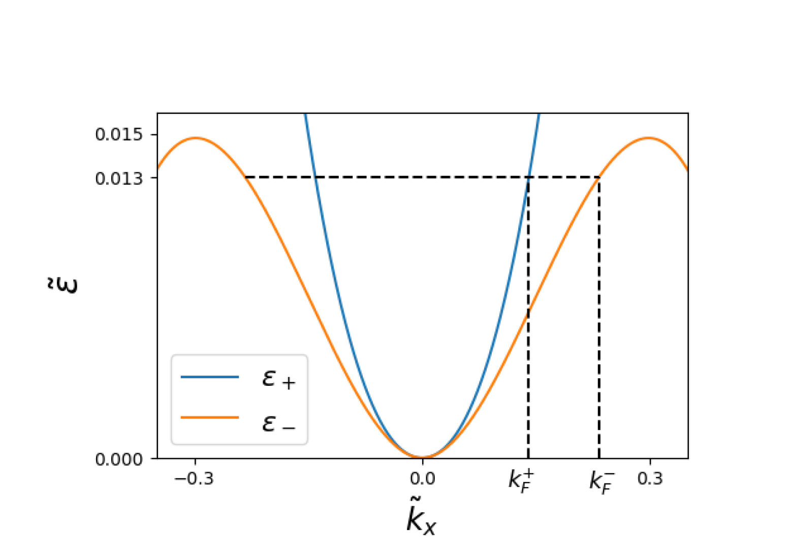
Figure 1: Two spin-split energy bands versus $\tilde{k}_{x}$ for $\beta=0.5\alpha$ are shown. Here $k_{F}^{\pm}$ are for a given Fermi energy.

In the following subsections, the first- and second-order intrinsic spin conductivity are calculated by numerically integrating the SBC and SBCP components over the $k$-space. To facilitate the numerics, the dispersion relation and all the velocity and spin current components are calculated in polar coordinates $(k,\phi)$. We have introduced dimensionless wave-vector $\tilde{k}=k/k_{h}$ with $k_{h}=\hbar^{2}/(m\alpha)$ and the dimensionless energy $\tilde{\varepsilon}=\varepsilon/\varepsilon_{h}$ with $\varepsilon_{h}=\alpha k_{h}^{3}$. The system parameters used for various plots are $\alpha=1\>\text{eVnm}^{3}$ and effective mass $m=0.41m_{e}$ with $m_{e}$ being the electron’s rest mass.

III.1 Spin Berry curvature and out-of-plane linear spin conductivity

The linear spin conductivity is calculated using the spin Berry curvature given in Eq.(22). The out-of-plane, transverse component of the SBC ($\Omega^{z}_{yx}$) is given by,

$$\Omega^{z}_{yx,\pm}=\mp\frac{3\sin\phi}{4k_{h}^{2}\tilde{k}^{3}}\left[\frac{3\cos\phi^{\prime}-2r(2\sin\psi-\sin\phi^{\prime})}{1+r^{2}-2r\sin(2\phi)}\right],$$ (31)

with the anisotropic parameter $r=\beta/\alpha$. Using Eqs.(12) and (31), we reproduce the known result for the intrinsic linear spin Hall conductivity in the pure Rashba case ($r=0$), which is $\chi^{z,R}_{yx}\simeq 9e/(8\pi)$ [26]. On the other hand, in the pure Dresselhaus case ($\alpha=0,\beta\neq 0)$, we get $\chi_{yx}^{z,D}\simeq 6e/(8\pi)$. Therefore, $\chi_{yx}^{z,D}$ is reduced by a factor of 2/3 as compared to $\chi_{yx}^{z,R}$. The linear spin Hall conductivity $\chi^{z}_{yx}$ is plotted as a function of the Fermi energy for different values of $r=\beta/\alpha$ in Fig. (2). The longitudinal spin conductivity $\chi^{z}_{xx}$ is zero in the pure Rashba and pure Dresselhaus cases. However, it is found to be non-zero in the presence of both Rashba and Dresselhaus interactions. For $r=0.5$, $\chi^{z}_{xx}\simeq 0.3331(9e/8\pi)$ and for $r=1.5$, $\chi^{z}_{xx}\simeq 0.2199(9e/8\pi)$. These spin conductivities vary only marginally with the Fermi energy.

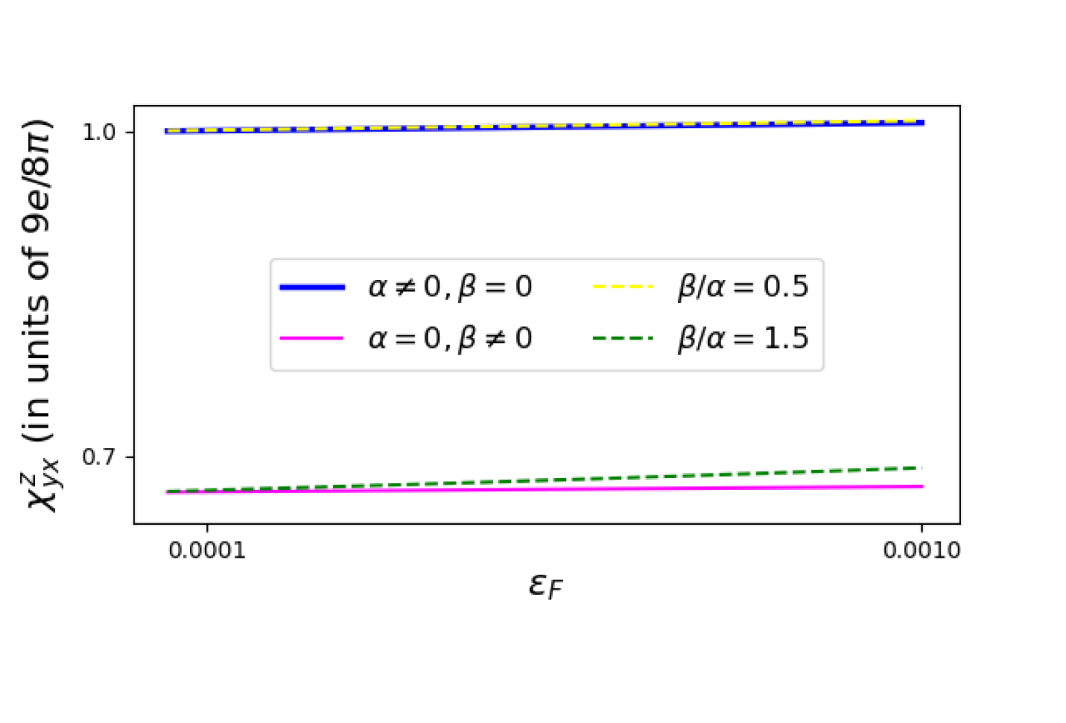
Figure 2: Linear spin Hall conductivity of the hole gas versus the scaled Fermi energy ($\varepsilon/\varepsilon_{h}$) for different values of $\beta/\alpha$.

III.2 Spin Berry curvature polarizability and in-plane second-order spin conductivity

Since the first-order spin conductivity is non-zero only when the spins are polarized out-of-plane, the first non-zero contribution from the in-plane spin current comes at the second-order. The in-plane components of the SBCP tensor are calculated according to Eq. (23). The electric field in the $x$ direction fixes the last two indices of the SBCP tensor at ’$x$’. These indices may be dropped for a simpler notation. Thus, we have four components with the spin being oriented either along the $x$ or $y$ direction.

$$\Pi^{x}_{x,\pm}=\Pi_{0}\left[\pm\cos\phi\cos\psi+\tilde{k}(3\sin 2\phi-2r(2+\cos 2\phi))\right],$$

$$\Pi^{y}_{y,\pm}=\Pi_{0}\left[\pm\sin\phi\sin\psi+\tilde{k}(3\sin 2\phi-2r(2-\cos 2\phi))\right],$$

$$\Pi^{x}_{y,\pm}=\Pi_{0}\left[\pm\sin\phi\cos\psi+\tilde{k}(3\cos 2\phi-2r\sin 2\phi)\right],$$

$$\Pi^{y}_{x,\pm}=\Pi_{0}\left[\pm\cos\phi\sin\psi-\tilde{k}(3\cos 2\phi-2r\sin 2\phi)\right],$$

where,

$$\Pi_{0}=\frac{3}{2\alpha k_{h}^{6}\tilde{k}^{7}}\left[\frac{3\cos\phi^{\prime}-2r(2\sin\psi-\sin\phi^{\prime})}{1+r^{2}-2r\sin(2\phi)}\right]^{2}.$$

In Fig. (3) the density plots of the SBCP components are shown. They have a multipolar nature; the $\Gamma^{x}_{x}$ and $\Gamma^{y}_{y}$ components being quadrupolar while $\Gamma^{x}_{y}$ and $\Gamma^{y}_{x}$ components are hexa-polar. In the absence of the Dresselhaus interaction (Fig. (3(a)) all four SBCP components are even functions in the $k$-space. Further, $\Gamma^{x}_{y}$ and $\Gamma^{y}_{x}$ are symmetric under reflection about the $k_{x}$ and $k_{y}$ axes, whereas $\Gamma^{x}_{x}$ and $\Gamma^{y}_{y}$ are anti-symmetric under such reflections. This property of the SBCP components can be in found in 2D electron gases as well [21]. The inclusion of the Dresselhaus term distorts the symmetric distributions as shown in Fig. (3(b)).

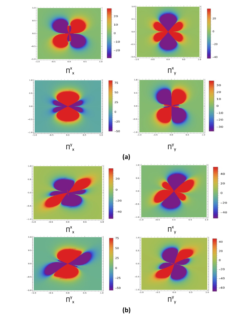
Figure 3: Density plots of the in-plane SBCP components for the $\varepsilon_{+}({\bf k})$ band in the $k_{x}$-$k_{y}$ plane: (a) pure Rashba case ($\beta=0$); (b) Rashba-Dresselhaus case ($\beta/\alpha=0.5$).

The intrinsic second-order in-plane spin conductivity is derived from the SBCP as shown in Eq. (13). They are plotted as functions of $\tilde{\varepsilon}_{F}$ in Fig. (4) along with the corresponding extrinsic components.

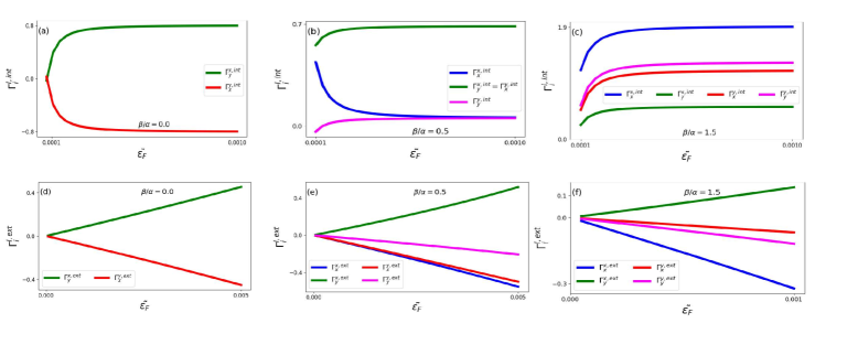
Figure 4: Second-order spin conductivity vs. Fermi energy (in units of $\varepsilon_{h}$). Top panel: variation of intrinsic second-order spin conductivity with Fermi energy for (a) $\beta/\alpha=0$ (b) $\beta/\alpha=0.5$ (c) $\beta/\alpha=1.5$. The scale of $\Gamma^{l,\text{int}}_{i}$ is set at $\Gamma_{0}\times 10^{8}$, with $\Gamma_{0}=e^{2}/(\alpha k_{h}^{4})$. Bottom panel: extrinsic contribution to second-order spin conductivity (in units of $\Gamma_{0}$) for (d) $\beta/\alpha=0$ (e) $\beta/\alpha=0.5$ (f) $\beta/\alpha=1.5$. The relaxation time $\tau$ is chosen to be $1\>\rm{ps}$.

When both the Rashba and Dresselhaus terms are present, all the four components of the second-order spin conductivity are non-zero. In the pure Rashba case, the components with the spin polarization and the spin current oriented in the same direction ($\Gamma^{x}_{x}$ and $\Gamma^{y}_{y}$) vanish, while other components ($\Gamma^{x}_{y}$ and $\Gamma^{y}_{x}$) survive. This is true for both the intrinsic and extrinsic cases. For 2D electron gases with $k$-linear Rashba interaction, the absence of $\Gamma^{x}_{x}$ and $\Gamma^{y}_{y}$ is attributed to the $\pi/2$ angle-locking between the spin polarization and the wave-vector ${\bf k}$. However, for the $k^{3}$ Rashba interaction studied here, the spins are not perpendicular to ${\bf k}$ everywhere in the $k$-space. They are perpendicular only at certain points, as shown in Appendix (A), where the Fermi contours are plotted along with the spin texture. Therefore, absence of $\Gamma^{x}_{x}$ and $\Gamma^{y}_{y}$ may not be due to the spin-momentum locking. The introduction of the Dresselhaus term makes the band structure anisotropic and allows the $\Gamma^{x}_{x}$ and $\Gamma^{y}_{y}$ components become finite as well. These components are however, very small for $\beta<\alpha$ and increases with the increase in $\beta$, as can be seen in Fig. (4(b,c)). Thus, the band anisotropic system such as Rashba-Dresselhaus spin-orbit coupling in 2DHG leads to the generation of all $\mathcal{T}$-allowed in-plane spin currents.

The extrinsic spin conductivity is contributed by the $\tau^{2}$-dependent term in Eq. (13) which is symmetric under $\mathcal{T}$. Unlike the electron gas [21] the extrinsic spin conductivity for the hole gas is found to increase with the Fermi energy. This can be understood by observing the difference in the dispersion curves of the electron gas and the hole gas. In the $k$-linear case the difference between the Fermi momenta of the two bands $(k_{F}^{+}-k_{F}^{-})$ does not change with the increase in the Fermi energy [7], whereas in case of $k$-cubic systems, as shown in Fig. (1), $(k_{F}^{+}-k_{F}^{-})$ increases with the Fermi energy. It has been shown in Appendix(B), at least in the pure Rashba limit, that the extrinsic spin conductivity depends on $(k_{F}^{+})^{2}-(k_{F}^{-})^{2}$ and hence, increases in magnitude with the Fermi energy. However, the magnitudes of the extrinsic components are negligibly small compared to the intrinsic ones. As shown in Fig. (4), $\Gamma^{l,\rm ext}_{i}/\Gamma^{l,\rm int}_{i}\sim 10^{-8}$. Hence, similar to the linear spin conductivity, the second-order spin conductivity is also dominated by the intrinsic contribution.

IV Two-dimensional hole gas with Rashba SOC subjected to linearly polarized electromagnetic radiation

As an alternative method of controlling the band anisotropy of the system, we irradiate linearly polarized electromagnetic radiation over the 2DHG with Rashba spin-orbit coupling. We consider a linearly polarized radiation with frequency $\omega$ and amplitude $A_{0}$ propagating perpendicular to the system. Using the Floquet-Magnus expansion [36] and taking the high-frequency limit, the final Hamiltonian becomes [37]

$$H=\frac{\hbar^{2}k^{2}}{2m}+i\alpha(k_{-}^{3}\sigma_{+}-k_{+}^{3}\sigma_{-})-\alpha A(\sigma_{x}k_{x}+\sigma_{y}k_{y}),$$ (32)

where $A=3(eA_{0}/\hbar)^{2}$. The energy dispersion is given by

$$\varepsilon(k)=\frac{\hbar^{2}k^{2}}{2m}\pm\alpha k\sqrt{(k^{2}-A\sin(2\phi))^{2}+A^{2}\cos^{2}(2\phi)}$$ (33)

with $\tan\phi=k_{y}/k_{x}$. The eigen spinors being,

$$|\pm\rangle=\frac{1}{\sqrt{2}}\begin{pmatrix}1\\ \pm e^{i\psi}\end{pmatrix},$$ (34)

where $\tan\psi=C/D$ with $C=A\sin\phi+k^{2}\cos(3\phi)$ and $D=A\cos\phi-k^{2}\sin(3\phi)$. The energy band gap is given by

$$\varepsilon_{g}=2\alpha k\sqrt{(k^{2}-A\sin(2\phi))^{2}+A^{2}\cos^{2}(2\phi)}.$$ (35)

There are degeneracy points at $k=\sqrt{A}$ with $\phi=(2p+1)\pi/4$ with $p=0,1,2,3$. We introduce dimensionless variables by scaling the $k$ by a typical wave-vector $k_{0}$ ($\tilde{k}=k/k_{0}$) and the energy is scaled by $\gamma=\hbar^{2}k_{0}^{2}/(2m)$ ($\varepsilon/\gamma$). Consequently, the other parameters get scaled as, $\tilde{A}=A/k_{0}^{2}$ and $\alpha_{0}=\alpha k_{0}^{3}/\gamma$.

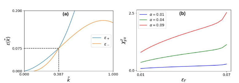
Figure 5: (a) Dispersion of Rashba spin-orbit coupled hole gas in the presence of electromagnetic radiation for $\phi=\pi/4$, $A=0.15$ and $\alpha_{0}=0.04$. The band degeneracy occurs at $\tilde{k}=0.387$ and the corresponding energy is about 0.075 in the given scale. (b) Linear spin Hall conductivity (in units of $e/\alpha_{0}$) as a function of the scaled Fermi energy ($\varepsilon/\gamma$) for different values of $\alpha$.

IV.1 Spin Berry curvature and linear spin conductivity

We already know that only the out-of-plane components of the SBC tensor will survive. Since, the electric field is along the $x$ direction, the spin Hall current is computed along the $y$ direction. The SBC turns out to be,

$$\Omega^{z}_{yx,\pm}=\mp\frac{3\sin\phi}{2\alpha_{0}k_{0}^{2}\tilde{k}}\left[\frac{3\tilde{k}^{2}\cos(2\phi-\psi)-\tilde{A}\sin\psi}{\tilde{k^{4}}+\tilde{A}^{2}-2\tilde{A}\tilde{k}^{2}\sin(2\phi)}\right].$$ (36)

The linear spin Hall conductivity $\chi^{z}_{yx}$ as a function of Fermi energy for different values of $\alpha_{0}$ is plotted in Fig. (5(b)). The spin Hall resonance occurs as the Fermi energy approaches the degeneracy. This has been previously studied in 2D electron and hole gases in the presence of external magnetic field [38, 39].

IV.2 Spin Berry curvature polarizability and second-order spin conductivity

Following the analysis done in sections (II) and (III), the SBCP components for the in-plane spin current are as follows:

$$\Pi^{x}_{x,\pm}=\Pi_{0}\left[\pm 4\tilde{k}\cos\phi\cos\psi+6\alpha_{0}\tilde{k}^{2}\sin(2\phi)+\alpha_{0}\tilde{A}\right],$$

$$\Pi^{y}_{y,\pm}=\Pi_{0}\left[\pm 4\tilde{k}\sin\phi\sin\psi+6\alpha_{0}\tilde{k}^{2}\sin(2\phi)+\alpha_{0}\tilde{A}\right],$$

$$\Pi^{x}_{y,\pm}=\Pi_{0}\left[\pm 4\tilde{k}\sin\phi\cos\psi+6\alpha_{0}\tilde{k}^{2}\cos(2\phi)\right],$$

$$\Pi^{y}_{x,\pm}=\Pi_{0}\left[\pm 4\tilde{k}\cos\phi\sin\psi-6\alpha_{0}\tilde{k}^{2}\cos(2\phi)\right],$$

where,

$$\Pi_{0}=\frac{3\alpha_{0}^{2}}{4\gamma k_{0}^{3}}\left[\frac{3\tilde{k}^{2}\cos(2\phi-\psi)-\tilde{A}\sin\psi}{\tilde{k^{4}}+\tilde{A}^{2}-2\tilde{A}\tilde{k}^{2}\sin(2\phi)}\right]^{2}.$$

The plots of the second-order intrinsic spin conductivity versus the Fermi energy are shown in Fig. (6(a)). The components appear to diverge as the energy approaches the resonance point, similar to the linear spin conductivity. The extrinsic contribution appears in the second-order spin conductivity from the non-linear Drude term in Eq. (13). The four in-plane components of the extrinsic spin conductivity are plotted against the Fermi energy in Fig. (6(b)). However, unlike section (III) here the intrinsic and extrinsic contributions are of equal magnitude. Fig. (6) also shows that these components have different peak values at resonance. They can have both positive and negative peaks, and the peaks obtained for the extrinsic case are slightly shifted from those obtained for the intrinsic case.

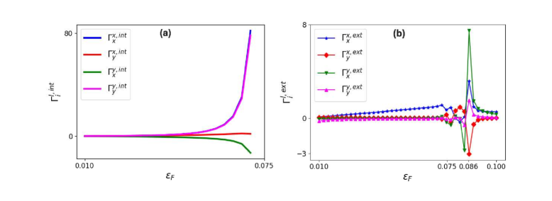
Figure 6: (a) Second-order intrinsic spin conductivity and (b) Second-order extrinsic spin conductivity (in units of $\Gamma_{\rm{em}}=e^{2}\alpha_{0}^{2}/(\gamma k_{0})$ as a function of the scaled Fermi energy. Here we have $\tau=1$ ps.

V Summary and conclusion

In this work, we have shown that the first non-vanishing in-plane spin current is non-linear (second-order), whereas the linear spin current is out-of-plane for any generic time-reversal symmetric 2D system. A summary of the vanishing and non-vanishing components of the linear and non-linear spin conductivity tensors are presented in Table (1). As a specific example, we considered two-dimensional heavy hole gas with spin-orbit interactions formed at the III-V semiconductor heterojunctions. It is shown that the linear spin Hall conductivity for pure Dresselhaus interaction ($\alpha=0,\beta\neq 0$) is reduced by a factor of 2/3, as compared to the pure Rashba interaction ($\alpha\neq 0,\beta=0$). The anisotropic Rashba-Dresselhaus spin-orbit interaction also induces a non-zero longitudinal spin conductivity, which otherwise vanishes in the isotropic, i.e. pure Rashba or pure Dresselhaus case. It is also observed that the linear spin conductivity for any combination of the spin-orbit interactions is nearly insensitive to the Fermi energy.

For the pure Rashba case, the second-order in-plane spin current is always normal to the spin-polarization. The band anisotropy, introduced by either the Dresselhaus spin-orbit interaction or an external electromagnetic field, generates additional second-order spin currents which are parallel to the spin-polarization. Therefore by tuning the ratio of the Rashba and Dresselhaus interaction strengths [40] or the amplitude of the electromagnetic radiation, the multiple in-plane spin currents can be controlled. The anisotropy may be used as a switch to turn on or off certain second-order spin currents that vanish in the pure Rashba limit . It has been further shown in Fig. (4) that the magnitudes of the spin conductivity components of such spin currents ($\Gamma^{x}_{x}$ and $\Gamma_{y}^{y}$) increase with increasing anisotropy. It is also observed that the extrinsic non-linear spin current is vanishingly small for the $k$-cubic hole gas with Rashba-Dresselhaus spin-orbit interaction, which is in contrast to the case for the $k$-linear 2D electron gas. However, in the presence of a linearly polarized electromagnetic radiation, the hole gas can host both extrinsic and intrinsic non-linear spin currents of equal magnitude. The electromagnetic radiation also causes spin-Hall resonance at a certain Fermi energy which can lead to a giant non-linear spin current. As discussed in section (IV), the different second-order spin currents (both extrinsic and intrinsic) can be distinguished based on their behaviour around the resonance point.

	In-plane				Out-of-plane
First-order	$\chi^{x}_{x}$	$\chi^{y}_{x}$	$\chi^{x}_{y}$	$\chi^{y}_{y}$	$\chi^{z}_{x}$	$\chi^{z}_{y}$
Isotropic	$\times$	$\times$	$\times$	$\times$	$\times$	$\checkmark$
Anisotropic	$\times$	$\times$	$\times$	$\times$	$\checkmark$	$\checkmark$
Second-order	$\Gamma^{x}_{x}$	$\Gamma^{y}_{x}$	$\Gamma^{x}_{y}$	$\Gamma^{y}_{y}$	$\Gamma^{z}_{x}$	$\Gamma^{z}_{y}$
Isotropic	$\times$	$\checkmark$	$\checkmark$	$\times$	$\times$	$\times$
Anisotropic	$\checkmark$	$\checkmark$	$\checkmark$	$\checkmark$	$\times$	$\times$
	Longitudinal		Transverse		Longitudinal	Transverse

Table 1: All the vanishing and non-vanishing components of the first- and second-order spin conductivity tensors.

Appendix A Spin polarization vector on the Fermi contours

The local spin polarization vector can be defined as ${\bf P}_{\pm}({\bf k})=\langle\pm|{\bf S}|\pm\rangle$, where the spin operator is given by ${\bf S}=(\hbar/2)(\sigma_{x},\sigma_{y})$. For 2D heavy hole gas, using the eigenspinors $(|\pm\rangle)$ given in section (III), we obtain

$${\bf P}_{\pm}({\bf k})=\pm\frac{\hbar}{2}(\cos\psi,\sin\psi),$$ (37)

where the explicit expressions of $\cos\psi$ and $\sin\psi$ are given by,

$$\cos\psi=\frac{\sin\phi(4\cos^{2}\phi-1)-r\cos\phi}{\sqrt{1+r^{2}-2r\sin(2\phi)}},$$ (38)

$$\sin\psi=\frac{\cos\phi(4\sin^{2}\phi-1)-r\sin\phi}{\sqrt{1+r^{2}-2r\sin(2\phi)}}.$$ (39)

Here $\psi=2\phi-\phi^{\prime}$.

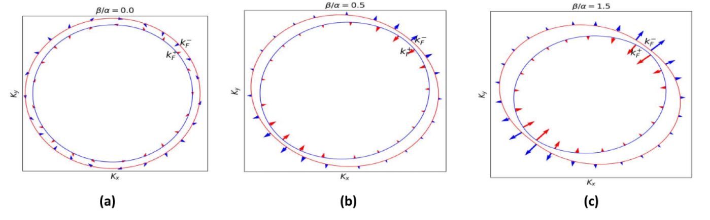
Figure 7: The local spin polarization vectors ${\bf P}_{\pm}({\bf k})$ on the Fermi contours of the 2D hole gas for $\beta/\alpha=0,0.5,1.5$.

The Fermi contours for the two bands and the local polarization vector ${\bf P}({\bf k})$ are shown in Fig. (7). Note that ${\bf P}({\bf k})$ is inversely proportional to the band gap $\varepsilon_{g}$. Therefore, the magnitude of ${\bf P}({\bf k})$ vector is large near the points where the band gap is small and it decreases with the increase of the band gap. It should be mentioned here that along $k_{y}=k_{x}$, for $\alpha=\beta$ the band gap vanishes but the spin polarization is finite: ${\bf P}_{\pm}=\pm\frac{\hbar}{2}(\frac{1}{\sqrt{2}},-\frac{1}{\sqrt{2}})$ and independent of ${\bf k}$ as well as the spin-orbit coupling strength. Further, in the pure Rashba case ($\beta=0$), we get ${\bf P}_{\pm}({\bf k})=\pm\frac{\hbar}{2}(\sin 3\phi,-\cos 3\phi)$, so ${\bf k\cdot P}=\pm\frac{\hbar k}{2}\sin 2\phi$. Therefore, the spin is normal to its momentum only for $\phi=0,\pi/2,\pi,3\pi/2$, as contrast to the two-dimensional electron gas with the linear Rashba spin-orbit interaction. It is mentioned in Ref. [21] that the absence of $\Gamma_{x}^{x}$ and $\Gamma_{y}^{y}$ for 2DEG with the $k$-linear Rashba interaction is due to the $\pi/2$ spin-momentum locking. However, this is not the case for 2DHG with the $k$-cubic Rashba interaction.

Appendix B Extrinsic spin current

The only extrinsic contribution to the spin current comes from the non-linear Drude term given by Eq. (13),

$$\Gamma^{l,\text{ext}}_{ij\kappa}=e^{2}\sum_{n}\int_{k}[d{\bf k}]\>j^{l}_{i,n}\frac{\tau^{2}}{\hbar^{2}}\frac{\partial^{2}f^{(0)}_{n}}{\partial k_{j}\partial{k}_{\kappa}}.$$ (40)

In our case the indices $j$ and $k$ are $x$. So dropping the indices $j,k$ and assuming the relaxation time $\tau$ is independent of energy, we can rewrite this equation as,

$$\Gamma^{l,\text{ext}}_{i,\pm}=\frac{e^{2}\tau^{2}}{(2\pi\hbar)^{2}}\int_{k}d^{2}k\>\langle\pm|\hat{j}^{l}_{i}|\pm\rangle\>\frac{\partial^{2}f^{(0)}}{\partial k_{x}^{2}}.$$

The derivative of the the Fermi-Dirac distribution at very low temperature is can be expressed as

$$\frac{\partial f^{(0)}}{\partial\varepsilon^{\pm}}\simeq-\delta(\varepsilon^{\pm}-\varepsilon_{F})=-\frac{\delta(k-k_{F}^{\pm})}{\left|\frac{\partial\varepsilon^{\pm}}{\partial k_{F}^{\pm}}\right|}.$$ (41)

Putting this in the above integral we get,

$$\Gamma^{l,\text{ext}}_{i,\pm}=\frac{e^{2}\tau^{2}}{(2\pi\hbar)^{2}}\int_{k}d^{2}k\>\frac{\partial}{\partial k_{x}}(\langle\pm|\hat{j}^{l}_{i}|\pm\rangle)\>\frac{\partial\varepsilon^{\pm}}{\partial k_{x}}\frac{\delta(k-k_{F}^{\pm})}{\left|\frac{\partial\varepsilon^{\pm}}{\partial k_{F}^{\pm}}\right|},$$ (42)

where integration by parts is used to shift one of the $k_{x}$ derivatives on to the current density. For simplicity, we take the pure Rashba limit where only $\Gamma^{x}_{y}$ and $\Gamma^{y}_{x}$ are non-zero. The integral is converted to polar coordinates, where the $k$-integral is killed by the delta function and the $\phi$-integral is straight-forward. It can be easily shown that,

$$\Gamma^{x,\text{ext}}_{y}\sim[(k_{F}^{+})^{2}-(k_{F}^{-})^{2}].$$ (43)

This shows that as $k_{F}^{\pm}$ increases with increasing Fermi energy, the difference between the Fermi wave-vectors also increases, which increases the second-order extrinsic spin conductivity.

References

- Dyakonov and Perel [1971] M. Dyakonov and V. Perel, Current-induced spin orientation of electrons in semiconductors, Physics Letters A 35, 459 (1971).
- Hirsch [1999] J. E. Hirsch, Spin Hall effect, Phys. Rev. Lett. 83, 1834 (1999).
- Bychkov and Rashba [1984] Y. A. Bychkov and E. I. Rashba, Oscillatory effects and the magnetic susceptibility of carriers in inversion layers, Journal of Physics C: Solid State Physics 17, 6039 (1984).
- Dresselhaus [1955] G. Dresselhaus, Spin-orbit coupling effects in Zinc blende structures, Phys. Rev. 100, 580 (1955).
- Schliemann et al. [2003] J. Schliemann, J. C. Egues, and D. Loss, Nonballistic spin-field-effect transistor, Phys. Rev. Lett. 90, 146801 (2003).
- Schliemann and Loss [2003] J. Schliemann and D. Loss, Anisotropic transport in a two-dimensional electron gas in the presence of spin-orbit coupling, Phys. Rev. B 68, 165311 (2003).
- Sinova et al. [2004] J. Sinova, D. Culcer, Q. Niu, N. A. Sinitsyn, T. Jungwirth, and A. H. MacDonald, Universal intrinsic spin Hall effect, Phys. Rev. Lett. 92, 126603 (2004).
- Gradhand et al. [2010] M. Gradhand, D. V. Fedorov, P. Zahn, and I. Mertig, Extrinsic spin Hall effect from first principles, Phys. Rev. Lett. 104, 186403 (2010).
- Smit [1955] J. Smit, The spontaneous Hall effect in ferromagnetics I, Physica 21, 877 (1955).
- Smit [1958] J. Smit, The spontaneous Hall effect in ferromagnetics II, Physica 24, 39 (1958).
- Berger [1970] L. Berger, Side-jump mechanism for the Hall effect of ferromagnets, Phys. Rev. B 2, 4559 (1970).
- Karplus and Luttinger [1954] R. Karplus and J. M. Luttinger, Hall effect in ferromagnetics, Phys. Rev. 95, 1154 (1954).
- Berry [1984] M. V. Berry, Quantal phase factors accompanying adiabatic changes, Proceedings of the Royal Society of London. A. Mathematical and Physical Sciences 392, 45 (1984).
- Murakami et al. [2004] S. Murakami, N. Nagosa, and S.-C. Zhang, non-abelian holonomy and dissipationless spin current in semiconductors, Phys. Rev. B 69, 235206 (2004).
- Das et al. [2023] K. Das, S. Lahiri, R. B. Atencia, D. Culcer, and A. Agarwal, Intrinsic nonlinear conductivities induced by the quantum metric, Phys. Rev. B 108, L201405 (2023).
- Sodemann and Fu [2015] I. Sodemann and L. Fu, Quantum nonlinear hall effect induced by Berry curvature dipole in time-reversal invariant materials, Phys. Rev. Lett. 115, 216806 (2015).
- Zhang et al. [2021] Z.-F. Zhang, Z.-G. Zhu, and G. Su, Theory of nonlinear response for charge and spin currents, Phys. Rev. B 104, 115140 (2021).
- Wang et al. [2021] C. Wang, Y. Gao, and D. Xiao, Intrinsic nonlinear Hall effect in antiferromagnetic tetragonal cumnas, Phys. Rev. Lett. 127, 277201 (2021).
- Liu et al. [2021] H. Liu, J. Zhao, Y.-X. Huang, W. Wu, X.-L. Sheng, C. Xiao, and S. A. Yang, Intrinsic second-order anomalous Hall effect and its application in compensated antiferromagnets, Phys. Rev. Lett. 127, 277202 (2021).
- Kapri et al. [2021] P. Kapri, B. Dey, and T. K. Ghosh, Role of Berry curvature in the generation of spin currents in Rashba systems, Phys. Rev. B 103, 165401 (2021).
- Zhang et al. [2024] Z.-F. Zhang, Z.-G. Zhu, and G. Su, Intrinsic second-order spin current, Phys. Rev. B 110, 174434 (2024).
- Hamamoto et al. [2017] K. Hamamoto, M. Ezawa, K. W. Kim, T. Morimoto, and N. Nagaosa, Nonlinear spin current generation in noncentrosymmetric spin-orbit coupled systems, Phys. Rev. B 95, 224430 (2017).
- Hayami et al. [2022] S. Hayami, M. Yatsushiro, and H. Kusunose, Nonlinear spin Hall effect in -symmetric collinear magnets, Phys. Rev. B 106, 024405 (2022).
- Murakami et al. [2003] S. Murakami, N. Nagaosa, and S.-C. Zhang, Dissipationless quantum spin current at room temperature, Science 301, 1348 (2003).
- Bernevig and Zhang [2005] B. A. Bernevig and S.-C. Zhang, Intrinsic spin Hall effect in the two-dimensional hole gas, Phys. Rev. Lett. 95, 016801 (2005).
- Schliemann and Loss [2005] J. Schliemann and D. Loss, Spin-hall transport of heavy holes in III-V semiconductor quantum wells, Phys. Rev. B 71, 085308 (2005).
- Liu et al. [2023] H. Liu, J. H. Cullen, and D. Culcer, Topological nature of the proper spin current and the spin-Hall torque, Phys. Rev. B 108, 195434 (2023).
- Wong and Mireles [2010] A. Wong and F. Mireles, Spin Hall and longitudinal conductivity of a conserved spin current in two dimensional heavy-hole gases, Phys. Rev. B 81, 085304 (2010).
- Kaestner et al. [2006] B. Kaestner, J. Wunderlich, T. Jungwirth, J. Sinova, K. Nomura, and A. MacDonald, Experimental observation of the spin-Hall effect in a spin–orbit coupled two-dimensional hole gas, Physica E: Low-dimensional Systems and Nanostructures 34, 47 (2006).
- Murakami [2004] S. Murakami, Absence of vertex correction for the spin Hall effect in -type semiconductors, Phys. Rev. B 69, 241202 (2004).
- Xiang et al. [2024] L. Xiang, F. Xu, L. Wang, and J. Wang, Classification of spin Hall effect in two-dimensional systems, Frontiers of Physics 19, 33205 (2024).
- Ashcroft and Mermin [1976] N. W. Ashcroft and N. D. Mermin, Solid State Physics (Holt-Saunders, 1976).
- Rashba [2003] E. I. Rashba, Spin currents in thermodynamic equilibrium: The challenge of discerning transport currents, Phys. Rev. B 68, 241315 (2003).
- Pal and Ghosh [2024] O. Pal and T. K. Ghosh, Polarization and third-order Hall effect in III-V semiconductor heterojunctions, Phys. Rev. B 109, 035202 (2024).
- Bulaev and Loss [2005] D. V. Bulaev and D. Loss, Spin relaxation and decoherence of holes in quantum dots, Phys. Rev. Lett. 95, 076805 (2005).
- Mananga and Charpentier [2011] E. S. Mananga and T. Charpentier, Introduction of the floquet-magnus expansion in solid-state nuclear magnetic resonance spectroscopy, The Journal of Chemical Physics 135, 044109 (2011).
- Bhattacharya and Islam [2021] A. Bhattacharya and S. F. Islam, Photoinduced spin-Hall resonance in a -Rashba spin-orbit coupled two-dimensional hole system, Phys. Rev. B 104, L081411 (2021).
- Shen et al. [2004] S.-Q. Shen, M. Ma, X. C. Xie, and F. C. Zhang, Resonant spin Hall conductance in two-dimensional electron systems with a Rashba interaction in a perpendicular magnetic field, Phys. Rev. Lett. 92, 256603 (2004).
- Ma and Liu [2006] T. Ma and Q. Liu, Sign changes and resonance of intrinsic spin Hall effect in two-dimensional hole gas, Applied Physics Letters 89, 112102 (2006).
- Nitta et al. [1997] J. Nitta, T. Akazaki, H. Takayanagi, and T. Enoki, Gate control of spin-orbit interaction in an inverted IGAs/IAAs heterostructure, Phys. Rev. Lett. 78, 1335 (1997).