The isotropy of cosmic expansion in the early and late Universe

Abstract

We test the isotropy of cosmic expansion by combining several probes for the first time, constructing full-sky maps of expansion rate variation using Type Ia supernovae, fundamental plane galaxies, and CMB temperature fluctuations. We find no hint of anisotropy or correlation between early- and late-Universe expansion across all systematic models. The 99% confidence upper limits on expansion rate anisotropy are 0.39% for low-redshift supernovae, 0.95% for high-redshift CMB, and 0.37% when combined at a 60-degree smoothing scale. A significant anomaly in the fundamental plane residual map may reflect systematics in the current DESI dataset, as evidenced by the absence of cross-correlation with other tracers and its correlation with spatial density variations.

I Introduction

The standard $\Lambda$CDM cosmological model assumes homogeneity and isotropy: that the laws of physics are invariant throughout the Universe and that the distribution of matter and energy is statistically uniform on large scales. A direct consequence is an isotropic cosmic expansion. The expansion history, $H(z)$, and its present-day value, the Hubble constant $H_{0}=100h$ km s^-1 Mpc^-1, are constrained by early-Universe temperature anisotropies of the Cosmic Microwave Background (CMB) and by late-Universe distance indicators such as Type Ia supernovae (SNe) and fundamental plane (FP) galaxies.

Yet two decades of CMB observations [1, 2, 3, 4, 5, 6, 7, 8] have revealed hints of statistical anomalies in the low-$\ell$ temperature multipoles. Low-redshift surveys have also raised questions about the nature of the recent cosmic acceleration [9, 10]. Furthermore, $h$ inferred from early-Universe CMB data remains in tension with that from local supernovae measurements [11, 12]. A non-uniform Hubble flow could potentially alleviate these tensions through scenarios such as vector field inflation, non-trivial topologies, or inhomogeneous dark energy [3, 13, 14, 15]. However, the scarcity of independent large-scale modes makes it difficult to quantify such anomalies precisely.

We test for anisotropy in the Hubble flow by combining information from both early- and late-Universe probes for the first time. Under $\Lambda$CDM, any directional variation in $H_{0}$ measurements should be consistent with statistical noise and cosmic variance and also uncorrelated between epochs. A significant violation of this null hypothesis would suggest new physics or previously unaccounted-for systematics. While Hubble flow isotropy has been examined in individual probes [16, 17, 18, 19, 20, 21, 22, 23], we systematically construct full-sky $h$ maps using SNe, FP, and CMB data and compare them with isotropic predictions. The SN and FP maps trace the local expansion ($z<1$), whereas the CMB map extrapolates the expected $h$ from the $z\approx 1100$ temperature fluctuations. Not only do they independently probe the isotropy of the low- and high-$z$ Hubble flow, but their cross-correlation also provides a robust test for any correlated signal between the early and late Universe.

II Hubble residual maps

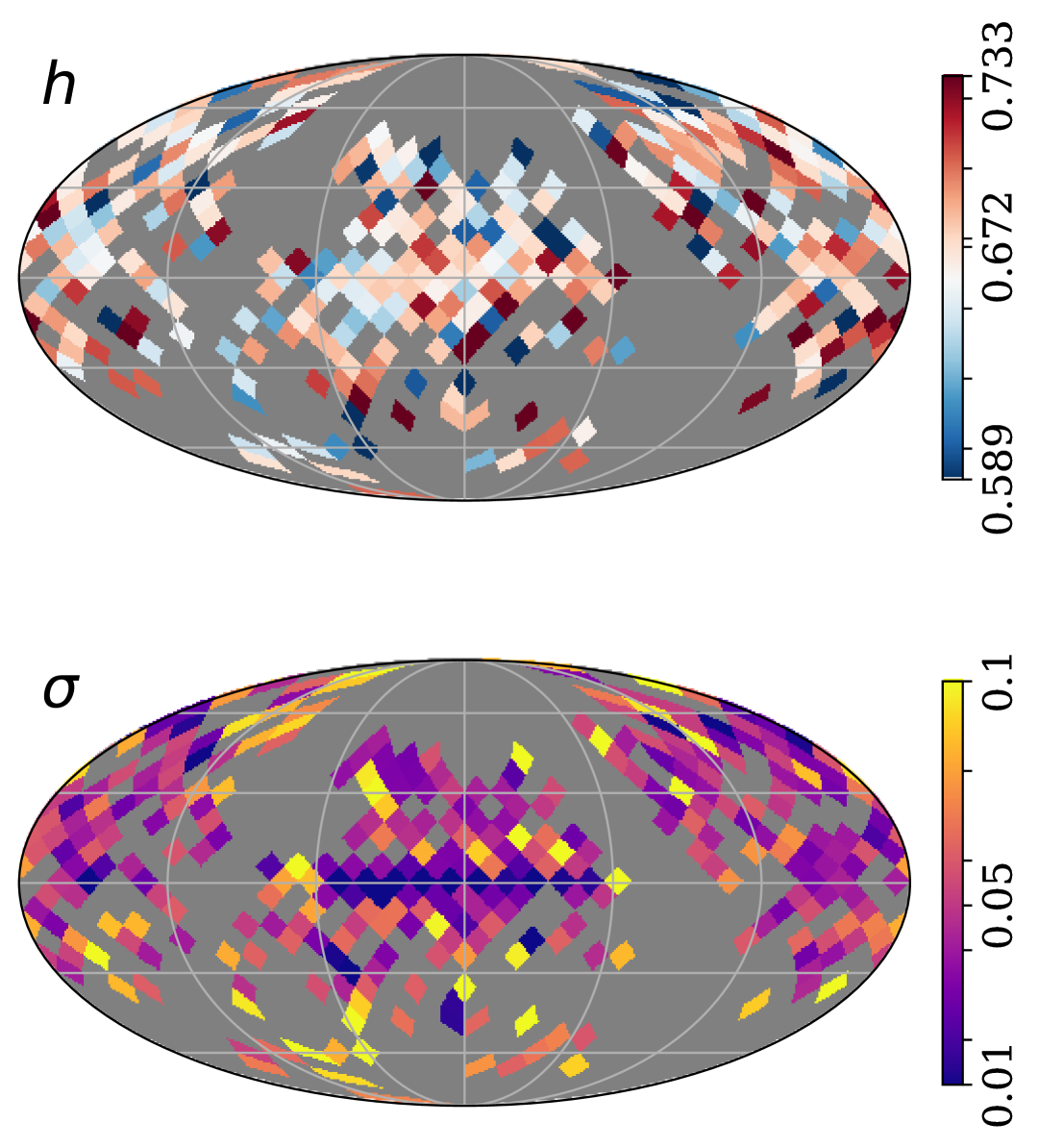
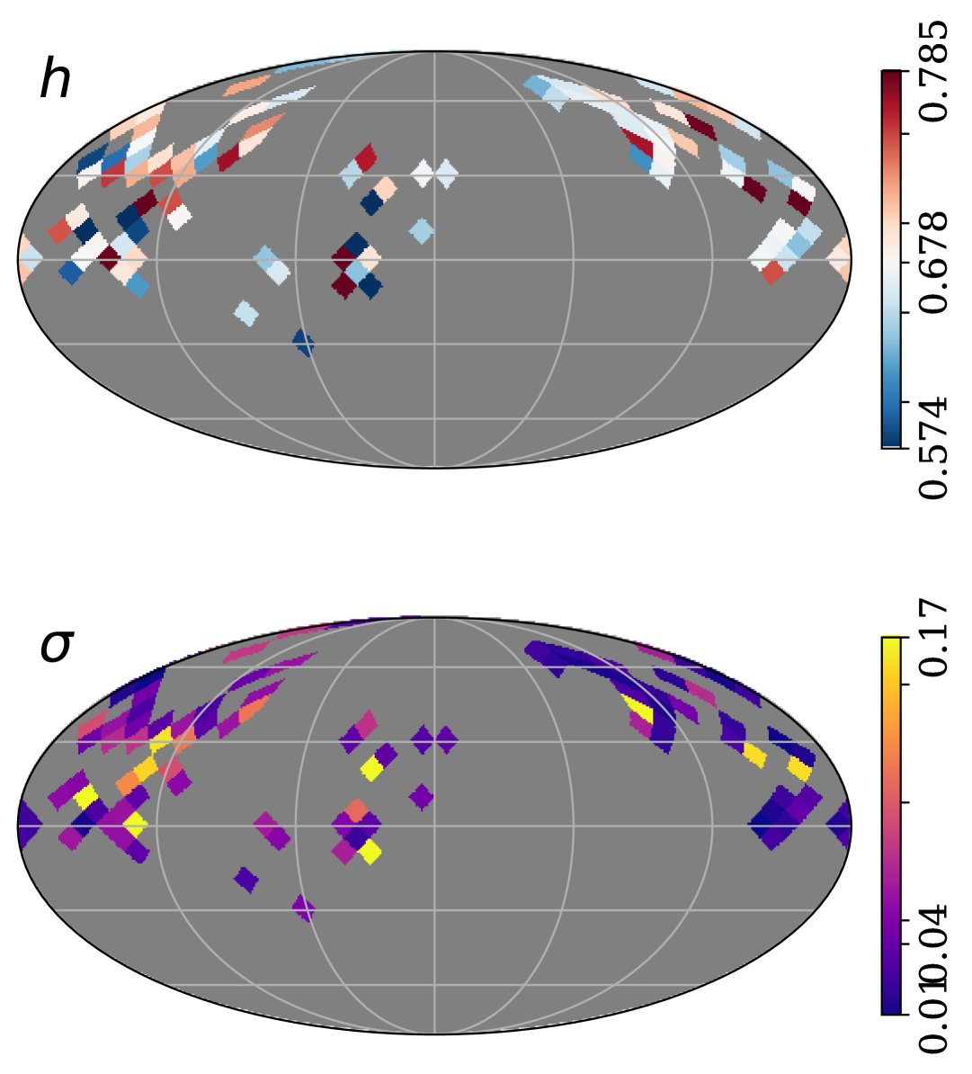
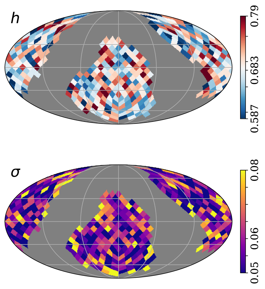
Figure 1: The $h$ and uncertainty $\sigma$ maps for supernovae (left), fundamental plane galaxies (middle) and CMB (right). All maps are calibrated to the Planck cosmology using fiducial analysis settings. Color bars mark the 5th, 50th and 95th percentiles. $f_{\text{sky}}=0.41,0.12,0.52$.

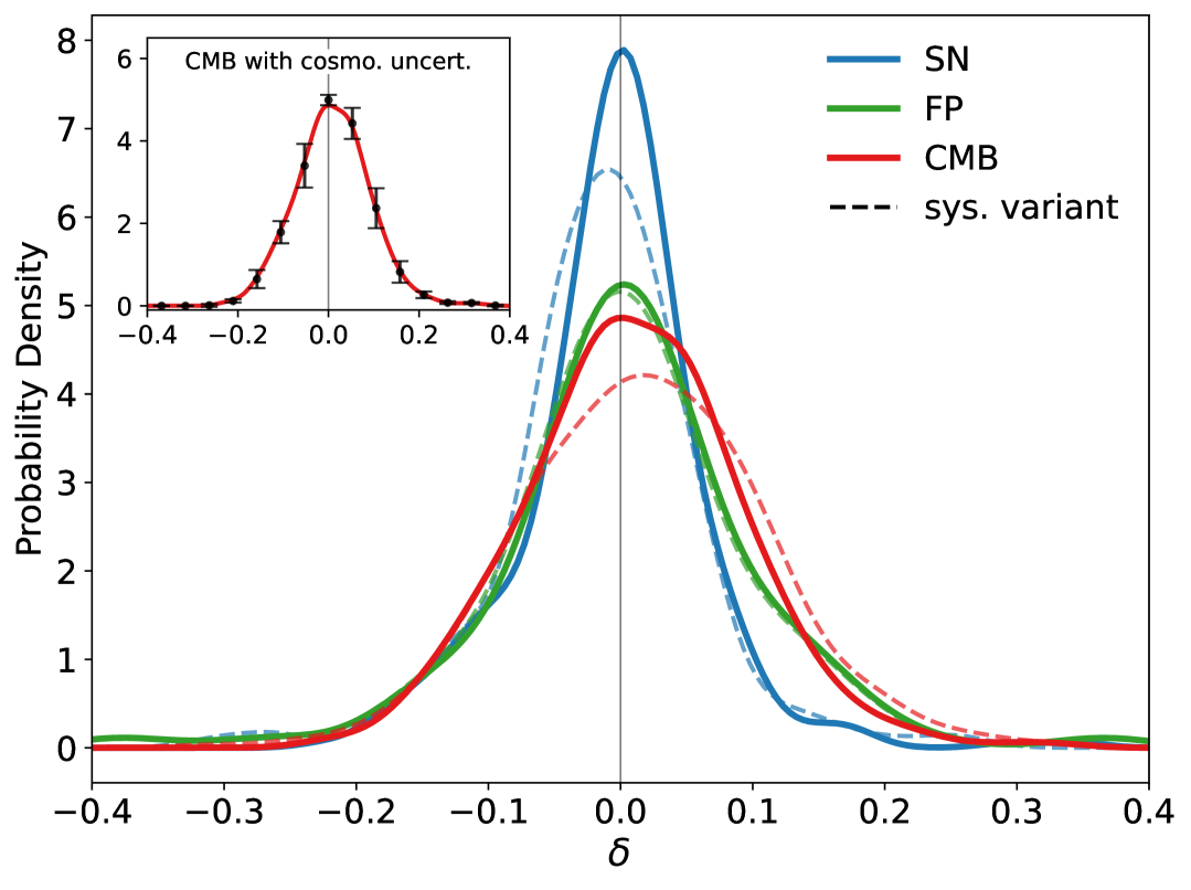
Figure 2: Pixel value histograms of $\delta_{\mathrm{SN}}$, $\delta_{\mathrm{FP}}$, and $\delta_{\mathrm{CMB}}$. Solid lines show fiducial configurations; dashed lines show systematic variants. The inset shows $\delta_{\mathrm{CMB}}$ histograms with error bars indicating 1$\sigma$ cosmological uncertainty. The distributions are zero-centered and approximately Gaussian. $\delta_{\mathrm{SN}}$ has the smallest scatter and $\delta_{\mathrm{CMB}}$ the largest.

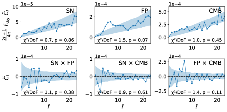
Figure 3: Weighted power spectra (Eq. 13) of the Hubble residual maps $\delta_{\rm SN}$, $\delta_{\rm FP}$, and $\delta_{\rm CMB}$. The weighted auto-power spectrum is scaled by $f_{\text{sky}}$ so that the area under the curve approximates the variance of the full-sky $\delta$ field. Solid lines represent the data, while shaded regions represent the 1$\sigma$ intervals of isotropic noise realizations. As indicated by the p-values in each panel, $\delta_{\mathrm{SN}}$ and $\delta_{\mathrm{CMB}}$ are consistent with isotropy, whereas the FP auto-power spectrum is not, with a significant peak around $\ell=6$.

Supernovae. Type Ia supernovae (SNe) are precise standardizable candles for cosmological distance measurements. The primary observable is the distance modulus $\mu=m-M$, where $m$ and $M$ are the apparent and standardized absolute magnitudes, respectively. For a supernova $i$ at scale factor $a_{i}$ (redshift $z_{i}$), the theoretical distance modulus $\mu_{\text{th},i}$ for a flat universe is

$$\mu_{\text{th},i} =5\log_{10}\left(\frac{c}{a_{i}}\int_{a_{i}}^{1}\frac{da^{\prime}}{a^{\prime 2}H(a^{\prime})}\right)+25\,,$$ (1)

where the argument of the log is the luminosity distance $d_{L}$ in Mpc. Equation 1 assumes an isotropic Hubble flow. We hypothesize that the difference between the observed $\mu_{i}$ and $\mu_{\text{th},i}$ arises from noise and potential anisotropy in the cosmic expansion. We model the latter as a perturbation to the Hubble parameter along the line of sight to each supernova

$$H_{0,i}=H_{0}(1+\delta_{i})\,.$$ (2)

In the limit of noiseless measurement, the distance modulus residual is directly proportional to the Hubble flow perturbation [19], since

$$\mu_{i}-\mu_{\text{th},i} =5\log_{10}\left(\int_{a_{i}}^{1}\frac{da^{\prime}}{a^{\prime 2}H_{i}(a^{\prime})}\Big{/}\int_{a_{i}}^{1}\frac{da^{\prime}}{a^{\prime 2}H(a^{\prime})}\right)$$ (3)

$$=-5\log_{10}\left(1+\delta_{i}\right)\approx-\frac{5\,\delta_{i}}{\ln 10}\,.$$ (4)

Equation 4 allows us to estimate $\delta_{i}$ and its uncertainty $\sigma_{i}$ from each supernova. Next, we directly construct a full sky $\delta$ map using the nside = 8 HEALPix pixelization scheme [24, 25] in contrast to the more indirect normalized residual approach of Soltis et al. [19]. The value and uncertainty of each pixel $p$ is given by the unbiased inverse variance estimator

$$\delta_{\text{SN}}(p)=\frac{\sum_{i\in p}\delta_{i}/\sigma_{i}^{2}}{\sum_{i\in p}1/\sigma_{i}^{2}}\,,\quad\sigma_{\text{SN}}(p)=\frac{1}{\sqrt{\sum_{i\in p}1/\sigma_{i}^{2}}}\,.$$ (5)

We analyze the Pantheon+SH0ES SNe data from Riess et al. [26] , originally calibrated via Cepheids to the absolute magnitude $M_{\text{fid}}=-19.24$ and yielding a global measurement of $h=0.7330$. Since we focus on the anisotropy rather than the absolute value of $h$ and wish to compare with other distance tracers, we recalibrate the SNe to the Planck 2018 CMB cosmology ($h=0.6736$ [27]), thereby changing the absolute magnitude to $M=-19.42$. The recalibration only centers the distribution of $h$ around $h_{\text{Planck}}$ but has no impact on our anisotropy results. We include 1701 SN with $z<2.3$ and median $z=0.164$. The $h$ and uncertainty maps are shown in Fig. 1, and the pixel histogram in Fig. 2. In the fiducial analysis, we consider supernova redshifts corrected for both the CMB dipole and the local group motion. The systematic variant where the redshift ($z_{\text{CMB}}$) is corrected only for the former is shown in Fig. 2 as the blue dashed curve.

Fundamental Plane Galaxies. Empirically, the physical radius of elliptical galaxies is related to their dynamical properties, and can thus be calibrated as a standardized ruler for distance and expansion rate measurements. This relationship, called the fundamental plane (FP), relates a galaxy’s effective radius $R_{e}$, central velocity dispersion $\sigma$, and mean surface brightness within $R_{e}$, $I_{e}$,

$$\log R_{e}=a\log\sigma+bI_{e}+c\,.$$ (6)

We analyze the DESI FP galaxy data [28], where $a$ and $b$ are calibrated to the observed galaxy population, and the zero-point $c$ is calibrated to the surface brightness fluctuation distance of the Coma cluster [28, 29]. We estimate each galaxy’s angular diameter distance $d_{A}$ (Mpc) by combining the FP-inferred physical radius $R_{e}$ (kpc) with the observed angular size $\theta_{e}$ (arcseconds),

$$k_{i}\equiv\log_{10}d_{A,i}=\log_{10}\left(\frac{R_{e,i}}{\theta_{e,i}}\cdot\frac{648}{\pi}\right)\,,$$ (7)

where $d_{A,i}$ is the angular diameter distance .

Analogous to the SNe analysis, if the expansion rate in direction $i$ deviates from the homogeneous background by a perturbation $\delta_{i}$ (Eq. 2), the observed angular diameter distance differs from the isotropic theory by

$$k_{i}-k_{\rm th,i} =\log_{10}\left(\int_{a_{i}}^{1}\frac{da^{\prime}}{a^{\prime 2}H_{i}(a^{\prime})}\Big{/}\int_{a_{i}}^{1}\frac{da^{\prime}}{a^{\prime 2}H(a^{\prime})}\right)$$ (8)

$$=\log_{10}\left(\frac{1}{1+\delta_{i}}\right)\approx-\frac{\delta_{i}}{\ln 10}\,.$$ (9)

Similar to the SNe, this distance measurement is also degenerate with $h$. Using $h=0.7605$ from the DESI analysis, we recalibrate $k_{i}$ to the Planck cosmology by $k_{i}\rightarrow k_{i}+\log_{10}(h_{\text{DESI}}/h_{\text{Planck}})$. The recalibration centers the distribution of $h$ around $h_{\text{Planck}}$.

We consider 4063 galaxies with $0.023<z<0.1$ and median $z=0.075$. We construct $\delta_{\rm FP}$ and $\sigma_{\rm FP}$ maps by inverse-variance averaging the FP galaxy measurements on a HEALPix grid (analogous to Eq. 5). The maps and the pixel histograms are shown in Figs. 1 and 2. The fiducial analysis corrects the redshift with the 2M++ peculiar velocity (PV) model [30], while a systematic variant does not.

The Cosmic Microwave Background. The CMB temperature power spectrum $C_{\ell}$ is another sensitive probe of $h$ [31, 27]. To construct the Hubble residual map, we partition the CMB temperature map into nside = 8 HEALPix pixels (labeled by $p$), measure the local power spectrum $C_{\ell}^{\text{local}}$, and finally estimate the residual $\delta_{\mathrm{CMB}}(p)=h(p)/h_{\text{Planck}}-1$ through a likelihood analysis.

We use the two Planck 2018 half-mission SMICA maps [32, 27], $T_{1}$ and $T_{2}$ with a resolution of nside = 1024. We use the combined 100, 143, and 217 GHz frequency masks ($f_{\mathrm{sky}}\approx 0.5$) to mitigate the impact of galactic foreground and point source contamination. For each pixel $p$, we gnomonically project $T_{1}$, $T_{2}$, and the masks to a Cartesian patch. We apodize the mask, measure the mode-decoupled $C_{\ell}$, and compute the Gaussian covariance of $C_{\ell}$, $\Sigma$, using pymaster [33]. Since the two half-mission temperature maps measure the same CMB structures but independent noise realizations, their cross-spectrum directly estimates the temperature auto-spectrum without noise bias.

For each sky patch, we estimate $h$ using a maximum-likelihood approach. The local spectrum is modeled as

$$C_{\ell}^{\rm local}=C_{\ell}^{\rm th}\cdot P_{\ell,1024}^{2}\cdot P_{\ell,\text{proj}}^{2}\cdot B_{\ell}^{2}\cdot T_{\ell,\text{SMICA}},$$ (10)

where $C_{\ell}^{\text{th}}$ is the LCDM prediction by camb [34], $P_{1024}$ and $P_{\text{proj}}$ are the pixel window functions of the HEALPix and the Cartesian projection, $B$ and $T_{\text{SMICA}}$ are the SMICA beam and transfer function [32]. Since we are interested in the Hubble flow and not the CMB physics, we fix all other parameters (including $\Omega_{m}h^{2},\Omega_{b}h^{2}$) and vary only $h$ as we compute the posterior

$$-\log\mathcal{P}(h)\propto\sum_{\ell,\ell^{\prime}}\left(C_{\ell}^{\text{obs}}-C_{\ell}^{\text{th}}(h)\right)\Sigma^{-1}_{\ell\ell^{\prime}}\left(C_{\ell^{\prime}}^{\text{obs}}-C_{\ell^{\prime}}^{\text{th}}(\theta)\right).$$ (11)

We construct the residual maps $\delta_{\mathrm{CMB}}(p)=h(p)/h_{\text{Planck}}-1$ and $\sigma_{\mathrm{CMB}}=\sigma(p)/h_{\text{Planck}}$. The maps and the pixel histograms are shown in Figs. 1 and 2.

In the fiducial analysis, we consider the scale cut $\ell\in[100,1250]$. A more conservative systematic analysis uses a more aggressive scale-cut $\ell\in[200,1000]$. Most of the $h$ sensitivity lies near the second acoustic peak at $\ell\approx 500$, which falls within both scale cuts. Larger scales exceed the patch size and are noisy; smaller scales are removed due to potential point source contamination. We also assess the impact of cosmological uncertainty in $\delta_{\mathrm{CMB}}$ by creating 1000 maps with cosmology sampled from the Planck posterior [27].

III Analysis

We jointly analyze the statistics of the three Hubble residual maps: $\delta_{\mathrm{SN}}$, $\delta_{\mathrm{FP}}$, and $\delta_{\mathrm{CMB}}$. To account for incomplete sky coverage and spatially varying measurement uncertainties, we focus on an inverse-variance weighted version of the $C_{\ell}$ statistics [33, 19],

$$\tilde{a}_{\ell m}^{\alpha} =\frac{\int M(\hat{\bf n})\delta_{\alpha}(\hat{\bf n})\sigma_{\alpha}^{-2}(\hat{\bf n})Y_{\ell m}^{*}(\hat{\bf n})\,d\Omega(\hat{\bf n})}{\int M(\hat{\bf n})\sigma_{\alpha}^{-2}(\hat{\bf n})\,d\Omega(\hat{\bf n})/4\pi}\,,$$ (12)

$$\tilde{C}_{\ell}^{\alpha,\beta} =\langle\tilde{a}_{\ell m}^{\alpha}\tilde{a}_{\ell m}^{\beta,*}\rangle_{m}\,,$$ (13)

where $\ell\in[1,23]$, $\alpha,\beta$ refer to SNe, FP, or CMB, and $M(\hat{\bf n})$ is the mask. Eqs. 12 and 13 are closely related to the standard $C_{\ell}$ statistics – if the unmasked data have spatially constant uncertainty and a flat power spectrum, Eq. 12 reduces to $\tilde{a}_{\ell m}=f_{\text{sky}}^{-1}\int M(\hat{\bf n})\delta(\hat{\bf n})Y_{\ell m}^{*}(\hat{\bf n})\,d\Omega(\hat{\bf n}),$ and the weighted power spectrum is related to the standard one by

$$C_{\ell}\approx f_{\text{sky}}\tilde{C}_{\ell}\,.$$ (14)

To test for isotropy, we extend the approach of Soltis et al. [19] to multiple tracers. Consider the set $\{(\delta(p),\sigma(p))\}$ for all unmasked pixels $p$. This distribution includes contributions from both the potentially anisotropic Hubble field and the underlying noise properties. For example, it captures how the spatially varying mask fraction of the CMB affects $\delta_{\mathrm{CMB}}$ and $\sigma_{\mathrm{CMB}}$, and how individual object measurement uncertainties and spatial number density variations affect the SNe and FP maps. For each $\delta$ map, we create 1000 isotropic noise realizations by drawing unmasked pixel values from this distribution. For each realization, we compute the auto- and cross-power spectra $\tilde{C}_{\ell}^{{\rm iso},\alpha\beta}$ among all tracers. Fig. 3 compares $\tilde{C}_{\ell}$ and $\tilde{C}_{\ell}^{{\rm iso},\alpha\beta}$ for the fiducial analysis choice.

To quantify the robustness of the isotropy assumption, we perform a $\chi^{2}$ test on the auto- and cross-spectra. We consider the multipole range $\ell\in[1,23]$ and estimate the covariance matrix from the isotropic noise realizations. To account for finite sample bias in the inverse covariance estimator, we apply the correction [35, 36]

$$\chi^{2}=\chi^{2}_{\rm raw}\times\frac{N_{\rm sim}-N_{\rm data}-2}{N_{\rm sim}-1}\,,$$ (15)

where $N_{\rm sim}$ is the number of isotropic simulations and $N_{\rm data}$ is the length of the data vector. Results are presented in Table 1 for both the fiducial analysis and three other models with different systematic treatments.

Configuration	$\chi^{2}$/DoF	$p$-value
Fiducial	0.921	0.6586
SN: $z_{\rm CMB}$	1.187	0.1423
CMB: scale-cut	0.961	0.5663
CMB: cosmo. uncert.	0.880	0.7457

Table 1: Results of the isotropy $\chi^{2}$ test using both the SNe and CMB tracers (DoF=66). The null hypothesis of isotropy is consistent for all variants shown, with the 3 lower rows each varying the systematic model of a single tracer.

The $p$-values of the individual auto- and cross-correlations among $\delta_{\mathrm{SN}}$ and $\delta_{\mathrm{CMB}}$ are shown in Fig. 3. We find that both are consistent with isotropy In Tab. 1, we present the $\chi^{2}$ of the joint analysis of $\delta_{\mathrm{SN}}$ and $\delta_{\mathrm{CMB}}$ and find that the fiducial model yields a $p$-value of 0.65, supporting the null hypotheses of (1) isotropic expansion and (2) uncorrelated expansion across epochs.

Fig. 3 shows that the auto-power spectrum of $\delta_{\mathrm{FP}}$ has a low p-value due to a significant excess around $\ell=6$ ($\theta\approx 30^{\circ}$), which is independent of the PV correction. However, since there is no significant cross-correlation between $\delta_{\mathrm{FP}}$ and $\delta_{\mathrm{SN}}$ (which cover the same low-redshift volume) and $\delta_{\mathrm{CMB}}$, we are reluctant to associate the FP anomaly with true cosmic anisotropy. Another reason against this association is that we find significant correlation between $\delta_{\mathrm{FP}}$ and the FP number density distribution (and to a lesser degree the mean redshift in each pixel) in the same $\ell$ range. This evidence for a possible systematic effect in the FP sample is robust across all aforementioned systematic choices. The current FP sample comprises only targets from the DESI science validation phase and has significant spatial depth variation across the sky, potentially inducing unaccounted-for selection effects. Future DESI data is expected to deliver more homogeneous coverage [37, 28].

To obtain an upper limit on the variance of the anisotropy, we follow the general approach of Soltis et al. [19] and decompose the observed $\delta$ into a true signal and noise, $\delta_{\mathrm{obs}}=\delta_{\mathrm{true}}+n$. Since $\delta_{\mathrm{obs}}$ for both SNe and CMB are consistent with isotropy, the noise must dominate $\delta_{\mathrm{obs}}$, thereby constraining the amplitude of $\delta_{\mathrm{true}}$. We construct this limit using both probes via the full-sky power spectrum. Since $\delta_{\mathrm{obs}}\approx n$, the 99% upper bound on the variance of the true $\delta$

$$\left\langle\delta_{\mathrm{true}}^{2}\right\rangle_{99\%}\;<\;\sum_{\ell}\frac{2\ell+1}{4\pi}\Bigl{(}C_{\ell}^{\rm iso}+2.33\,\Delta C_{\ell}^{\rm iso}\Bigr{)}\,B_{\ell}^{2}\,d\ell\,,$$ (16)

where $C_{\ell}^{\rm iso}$ and $\Delta C_{\ell}^{\rm iso}$ are the mean and scatter of the power spectrum of the full-sky isotropic noise, and $B_{\ell}$ smooths the map via a Gaussian beam. We derive this limit for the SNe, CMB, and inverse-variance combined maps on their joint footprint for scales between 10 and 120 degrees in Fig. 4. At 60 degrees, the 99% confidence limits on low-$z$ and high-$z$ anisotropy are 0.39% and 0.95% respectively, and 0.37% when combined.

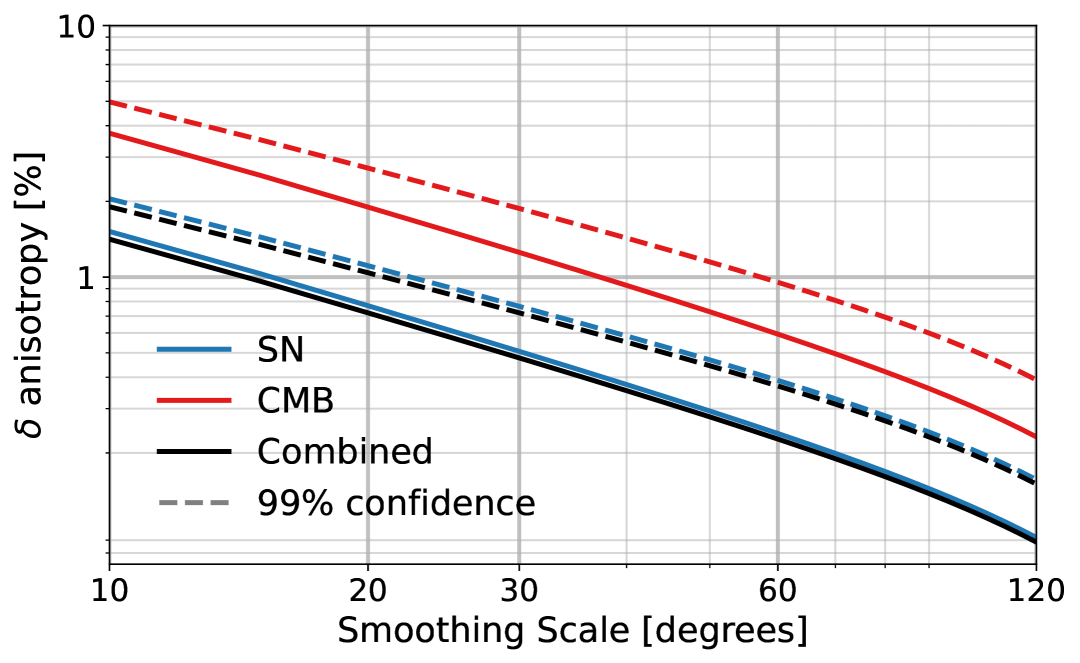
Figure 4: Upper limits on Hubble constant anisotropy as a function of smoothing scale. Solid lines show the mean noise level from isotropic realizations, while dashed lines indicate 99% confidence upper limits for the SNe, CMB, and the combined maps.

IV Conclusion

We tested the isotropy of cosmic expansion using three independent distance tracers: Type Ia supernovae, fundamental plane galaxies, and CMB temperature fluctuations. Aside from a localized anomaly in the FP auto-power spectrum around $\ell=6$, all measurements are consistent with isotropic expansion at low and high redshift, and results are robust across the systematic modeling choices we tested. The SNe and CMB measurements yield stringent constraints on potential Hubble flow anisotropy, with 99% confidence upper limits of 0.39% for low-redshift SNe, 0.95% for high-redshift CMB, and 0.37% when combined at a 60-degree smoothing scale.

We argue that – given this other evidence – it is premature to claim that the FP anomaly is a sign of genuine cosmic anisotropy. This hesitance is supported by the absence of significant cross-correlation between $\delta_{\mathrm{FP}}$ and the other tracers, particularly with $\delta_{\mathrm{SN}}$ which probes the same low-redshift volume, and by the correlation between $\delta_{\mathrm{FP}}$ and the spatial distribution of FP galaxy density. Future DESI data releases with more homogeneous sky coverage should shed light on this anomaly.

Acknowledgments. AZ thanks Yuuki Omori for insightful help with the Planck data, and Rachel Mandelbaum for early discussions. AZ is supported by the Jane Street Graduate Research Fellowship. This work was supported by FermiForward Discovery Group, LLC, under Contract No. 89243024CSC000002 with the U.S. Department of Energy, Office of Science, Office of High Energy Physics. D.S. acknowledges support from Department of Energy grant DE-SC0010007, the David and Lucile Packard Foundation, and the Templeton Foundation grant focused on understanding motions in the nearby universe.

References

- Hinshaw et al. [2003] G. Hinshaw, D. N. Spergel, et al., The Astrophysical Journal Supplement Series 148, 135 (2003), arXiv:astro-ph/0302217 .
- Spergel et al. [2003] D. N. Spergel, L. Verde, et al., The Astrophysical Journal Supplement Series 148, 175 (2003).
- De Oliveira-Costa et al. [2004] Angélica De Oliveira-Costa, Max Tegmark, et al., Physical Review D 69, 063516 (2004).
- Eriksen et al. [2005] H. K. Eriksen, A. J. Banday, et al., The Astrophysical Journal 622, 58 (2005).
- Land and Magueijo [2005] Kate Land and Joao Magueijo, Physical Review Letters 95, 071301 (2005), arXiv:astro-ph/0502237 .
- Copi et al. [2010] Craig J. Copi, Dragan Huterer, et al., Advances in Astronomy 2010, 847541 (2010), arXiv:1004.5602 [astro-ph, physics:gr-qc, physics:hep-th] .
- Bennett et al. [2011] C. L. Bennett, R. S. Hill, et al., The Astrophysical Journal Supplement Series 192, 17 (2011), arXiv:1001.4758 [astro-ph] .
- Collaboration et al. [2020a] Planck Collaboration, Y. Akrami, et al., Astronomy & Astrophysics 641, A7 (2020a), arXiv:1906.02552 [astro-ph] .
- Collaboration et al. [2025a] DESI Collaboration, A. G. Adame, et al., Journal of Cosmology and Astroparticle Physics 2025 (02), 021, arXiv:2404.03002 [astro-ph] .
- Collaboration et al. [2025b] DESI Collaboration, M. Abdul-Karim, et al., DESI DR2 Results II: Measurements of Baryon Acoustic Oscillations and Cosmological Constraints (2025b), arXiv:2503.14738 [astro-ph] .
- Valentino et al. [2021] Eleonora Di Valentino, Olga Mena, et al., Classical and Quantum Gravity 38, 153001 (2021), arXiv:2103.01183 [astro-ph] .
- Kamionkowski and Riess [2022] Marc Kamionkowski and Adam G. Riess, The Hubble Tension and Early Dark Energy (2022), arXiv:2211.04492 [astro-ph] .
- Copeland et al. [2006] Edmund J. Copeland, M. Sami, et al., International Journal of Modern Physics D 15, 1753 (2006), arXiv:hep-th/0603057 .
- Cooray et al. [2010] Asantha Cooray, Daniel E. Holz, et al., Journal of Cosmology and Astroparticle Physics 2010 (11), 015, arXiv:0812.0376 [astro-ph] .
- Maleknejad et al. [2013] A. Maleknejad, M. M. Sheikh-Jabbari, et al., Physics Reports 528, 161 (2013), arXiv:1212.2921 [hep-th] .
- Colin et al. [2011] Jacques Colin, Roya Mohayaee, et al., Monthly Notices of the Royal Astronomical Society 414, 264 (2011), arXiv:1011.6292 [astro-ph] .
- Kim and Komatsu [2013] Jaiseung Kim and Eiichiro Komatsu, Physical Review D 88, 101301 (2013), arXiv:1310.1605 [astro-ph] .
- Saadeh et al. [2016] Daniela Saadeh, Stephen M. Feeney, et al., Physical Review Letters 117, 131302 (2016), arXiv:1605.07178 [astro-ph] .
- Soltis et al. [2019] John Soltis, Arya Farahi, et al., Physical Review Letters 122, 091301 (2019).
- Fosalba and Gaztanaga [2021] Pablo Fosalba and Enrique Gaztanaga, Monthly Notices of the Royal Astronomical Society 504, 5840 (2021), arXiv:2011.00910 [astro-ph] .
- Yeung and Chu [2022] S. Yeung and M. C. Chu, Physical Review D 105, 083508 (2022).
- Haridasu et al. [2024] Balakrishna S. Haridasu, Paolo Salucci, et al., Radial Tully-Fisher relation and the local variance of Hubble parameter (2024), arXiv:2403.06859 [astro-ph] .
- Gimeno-Amo et al. [2025] C. Gimeno-Amo, F. K. Hansen, et al., Exploring Statistical Isotropy in Planck Data Release 4: Angular Clustering and Cosmological Parameter Variations Across the Sky (2025), arXiv:2504.05597 [astro-ph] .
- Gorski et al. [2005] K. M. Gorski, E. Hivon, et al., The Astrophysical Journal 622, 759 (2005), arXiv:astro-ph/0409513 .
- Zonca et al. [2019] Andrea Zonca, Leo Singer, et al., Journal of Open Source Software 4, 1298 (2019).
- Riess et al. [2022] Adam G. Riess, Wenlong Yuan, et al., The Astrophysical Journal Letters 934, L7 (2022), arXiv:2112.04510 [astro-ph] .
- Collaboration et al. [2020b] Planck Collaboration, N. Aghanim, et al., Astronomy & Astrophysics 641, A6 (2020b), arXiv:1807.06209 [astro-ph] .
- Said et al. [2024] Khaled Said, Cullan Howlett, et al., DESI Peculiar Velocity Survey – Fundamental Plane (2024), arXiv:2408.13842 [astro-ph] .
- Jensen et al. [2021] Joseph B. Jensen, John P. Blakeslee, et al., The Astrophysical Journal Supplement Series 255, 21 (2021).
- Said et al. [2020] Khaled Said, Matthew Colless, et al., Monthly Notices of the Royal Astronomical Society 497, 1275 (2020).
- Dodelson [2003] Scott Dodelson, Modern Cosmology (Academic Press, San Diego, Calif, 2003).
- Collaboration et al. [2020c] Planck Collaboration, Y. Akrami, et al., Astronomy & Astrophysics 641, A4 (2020c), arXiv:1807.06208 [astro-ph] .
- Alonso et al. [2019] David Alonso, Javier Sanchez, et al., Monthly Notices of the Royal Astronomical Society 484, 4127 (2019), arXiv:1809.09603 [astro-ph] .
- Lewis et al. [2000] Antony Lewis, Anthony Challinor, et al., The Astrophysical Journal 538, 473 (2000), arXiv:astro-ph/9911177 .
- Hartlap et al. [2009] J. Hartlap, T. Schrabback, et al., Astronomy & Astrophysics 504, 689 (2009), arXiv:0901.3269 [astro-ph] .
- Dodelson and Schneider [2013] Scott Dodelson and Michael D. Schneider, Physical Review D 88, 063537 (2013), arXiv:1304.2593 [astro-ph] .
- Saulder et al. [2023] Christoph Saulder, Cullan Howlett, et al., Monthly Notices of the Royal Astronomical Society 525, 1106 (2023).