Exact plane symmetric black bounce with a perfect-fluid exterior
obeying a linear equation of state

Abstract

We investigate an exact two-parameter family of plane symmetric solutions admitting a hypersurface-orthogonal Killing vector in general relativity with a perfect fluid obeying a linear equation of state $p=\chi\rho$ in $n(\geq 4)$ dimensions, obtained by Gamboa in 2012. The Gamboa solution is identical to the topological Schwarzschild-Tangherlini-(anti-)de Sitter $\Lambda$-vacuum solution for $\chi=-1$ and admits a non-degenerate Killing horizon only for $\chi=-1$ and $\chi\in[-1/3,0)$. We identify all possible regular attachments of two Gamboa solutions for $\chi\in[-1/3,0)$ at the Killing horizon without a lightlike thin shell, where $\chi$ may have different values on each side of the horizon. We also present the maximal extension of the static and asymptotically topological Schwarzschild-Tangherlini Gamboa solution, realized only for $\chi\in(-(n-3)/(3n-5),0)$, under the assumption that the value of $\chi$ is unchanged in the extended dynamical region beyond the horizon. The maximally extended spacetime describes either (i) a globally regular black bounce whose Killing horizon coincides with a bounce null hypersurface, or (ii) a black hole with a spacelike curvature singularity inside the horizon. The matter field inside the horizon is not a perfect fluid but an anisotropic fluid that can be interpreted as a spacelike (tachyonic) perfect fluid. A fine-tuning of the parameters is unnecessary for the black bounce but the null energy condition is violated everywhere except on the horizon. In the black-bounce (black-hole) case, the metric in the regular coordinate system is $C^{\infty}$ only for $\chi=-1/(1+2N)$ with odd (even) $N$ satisfying $N>(n-1)/(n-3)$, and if one of the parameters in the extended region is fine-tuned.

I Introduction

The interior structure of a realistic black hole is a highly nontrivial problem. Although curvature singularities exist inside the Schwarzschild and Kerr vacuum black holes in general relativity, it is widely believed that the quantum effects of gravity are so dominant near the singularity that singularities do not exist as a configuration of spacetime in full quantum gravity. Since the theory of quantum gravity is still incomplete at present, many models of singularity-free black holes have been proposed based on the belief that such non-singular black holes are realized even in the classical theory as a low-energy limit of quantum gravity.

Among various types of non-singular black holes, the type with a regular center has been studied in the most detail until now. (See Sec. 2.2 in Ref. Maeda:2021jdc for a review.) In Ref. Maeda:2021jdc , one of the authors proposed seven criteria to single out physically reasonable non-singular black-hole models and studied the models by Bardeen Bardeen1968 , Hayward Hayward2006 , Dymnikova Dymnikova:2004zc , and Fan and Wang Fan:2016hvf . Although this type of non-singular black hole with a regular center can be an exact solution to the Einstein equations with a nonlinear electromagnetic field AyonBeato:2000zs , the integration constants must be fine-tuned to remove the singularity at the center Chinaglia:2017uqd . (See also Appendix A in Ref. Maeda:2021jdc .) Therefore, such non-singular black holes are not generic configurations of black holes in that system, which does not meet one of the criteria proposed in Ref. Maeda:2021jdc . Nevertheless, a modified theory of gravity is known in which electrically charged spherically symmetric black holes are generally singularity-free Cano:2020ezi . Moreover, it was shown that such non-singular black holes can be generic even in pure gravity Bueno:2024dgm .

On the other hand, besides the regular-center type, there is an interesting type of non-singular black hole, in which a singularity is avoided by the big bounce which occurs on a spacelike or null hypersurface in the dynamical region inside the horizon. Such a black hole is referred to as a black universe by Bronnikov, Melnikov, and Dehnen Bronnikov:2006fu . However, a catchy name “black bounce” introduced later by Simpson and Visser Simpson:2018tsi for such black holes is more popular today. The black bounce may be more promising than the regular-center type in that it is not necessarily accompanied by an inner horizon, which is inevitable in the regular-center type and could suffer from the mass inflation instability Poisson:1989zz ; Poisson:1990eh ; Ori:1991zz . (See Refs. Rubio:2021obb ; Bonanno:2020fgp ; DiFilippo:2022qkl ; Carballo-Rubio:2022kad ; Carballo-Rubio:2024dca for recent studies of the inner-horizon instability of the regular-center type.)

A black bounce has been realized as solutions with a variety of matter fields: a minimally coupled ghost scalar field with potential Bronnikov:2005gm and with a Maxwell field Bolokhov:2012kn , a non-minimally coupled scalar field with potential Bronnikov:2022gjq , a conformally coupled scalar field with potential and a Maxwell field Barrientos:2022avi , a nonlinear electromagnetic field and a minimally coupled scalar field with potential Canate:2022gpy ; Bronnikov:2022bud ; Rodrigues:2023vtm ; Bronnikov:2023aya ; Alencar:2024yvh , a phantom scalar field that is non-minimally coupled to the Maxwell field Huang:2019arj ; Yang:2021diz , and $k$-essence theory, namely a scalar field with a non-canonical kinetic term Pereira:2023lck ; Pereira:2024gsl ; Pereira:2024rtv . Black-bounce configurations that generalize the Simpson-Visser spacetime can be found in Refs. Lobo:2020ffi ; Franzin:2021vnj ; Bronnikov:2021uta ; Lessa:2024erf . Apart from general relativity black-bounce spacetimes have been found in modified theories of gravity Junior:2022zxo ; Fabris:2023opv ; Junior:2024vrv ; Junior:2024cbb and in lower dimensions Furtado:2022tnb . More studies concerning black bounces in the context of astrophysics are such as quasinormal modes Churilova:2019cyt ; Franzin:2022iai ; Wu:2022eiv , shadows Guerrero:2021ues ; Guo:2021wid ; Lima:2021las , and gravitational lensing Nascimento:2020ime ; Tsukamoto:2020bjm ; Islam:2021ful ; Tsukamoto:2021caq ; Cheng:2021hoc .

In this paper, we present an exact black-bounce solution in general relativity in $n(\geq 4)$ dimensions with one of the simplest matter fields, a perfect fluid obeying a linear equation of state, instead of more complex matter fields as in most of the references previously cited. Such a simple black bounce can be achieved by a careful analysis of the causal and global structures of a static solution with planar symmetry found by Gamboa in Ref. GamboaSaravi

The organization of this paper is as follows. In Sec. II, we present a new form of the Gamboa solution GamboaSaravi and review several physical and mathematical concepts for the subsequent sections. In Sec. III, we identify all possible regular attachments of two Gamboa solutions at a non-degenerate Killing horizon and derive the conditions for the $C^{\infty}$ attachment. In Sec. IV, we clarify the maximally extended spacetimes of the static Gamboa solution for $\chi\in(-(n-3)/(3n-5),0)$ under the assumption that the value of $\chi$ is unchanged in the extended dynamical region beyond the horizon. Our main results are summarized in the final section. In Appendix A, we present another derivation of the Gamboa solution generalizing the original one with an $(n-2)$-dimensional Ricci-flat base manifold. In Appendix B, we show the regularity of the bifurcation $(n-2)$-surface in the solution. In Appendix C, we derive an explict form of the matter field confined on the Killing horizon in the solution for $\chi=-1/3$.

Our conventions for curvature tensors are $[\nabla_{\rho},\nabla_{\sigma}]V^{\mu}={{R}^{\mu}}_{\nu\rho\sigma}V^{\nu}$ and ${R}_{\mu\nu}={{R}^{\rho}}_{\mu\rho\nu}$, where Greek indices run over all spacetime indices. The signature of the Minkowski spacetime is $(-,+,+,\cdots,+)$. We adopt the units such that $c=1$ and $\kappa_{n}:=8\pi G_{n}$, where $G_{n}$ is the $n$-dimensional gravitational constant.

II Exact perfect-fluid solution for $p=\chi\rho$ ($\chi\neq 0,1$) with plane symmetry

In this paper, we study an exact static solution to the following Einstein equations with a perfect fluid obeying $p=\chi\rho$ in $n(\geq 4)$ dimensions:

$$\begin{aligned} &G_{\mu\nu}=\kappa_{n}T_{\mu\nu},\\ &{T}_{\mu\nu}=(\rho+p)u_{\mu}u_{\nu}+pg_{\mu\nu}.\end{aligned}$$ (1)

Here $\rho$ and $p$ are the energy density and pressure of a perfect fluid, respectively, and $u^{\mu}$ is the normalized $n$-velocity of the fluid element satisfying $u_{\mu}u^{\mu}=-1$.

The general static solution with planar symmetry in this system was obtained by Gamboa GamboaSaravi . In Appendix A, using a different coordinate system, we present a simple derivation of the Gamboa solution and its generalization by considering an arbitrary Ricci-flat base manifold instead of just $\mathbb{R}^{n-2}$. However, in the present work, this generalization is not considered and the base manifold is chosen as the $(n-2)$-dimensional flat space to preserve planar symmetry, whose line element is denoted by ${\rm d}l_{n-2}^{2}$.

II.1 New form of the Gamboa solution for $\chi\neq 0,1$ with $A_{0}\neq 0$

We are interested in the general case of the Gamboa solution for $\chi\neq 0,1$ since there is no static solution for $\chi=0$ and the solution does not admit a Killing horizon for $\chi=1$. The forms of the Gamboa solution are different for $\chi=\chi_{0}$ and $\chi\neq\chi_{0}$, where

$$\chi_{0}:=-\frac{n-3}{3n-5}\left(>-\frac{1}{3}\right).$$ (2)

(See Eq. (100).) By the following coordinate transformation and reparametrizations

$$\begin{aligned} &T\to A_{0}^{(1+\beta)/(2+\beta)}B_{0}^{-1/2}T,\\ &M:=-A_{0}^{(3+2\beta)/(2+\beta)}/(2B_{0}),\\ &h_{1}:=-A_{1}/A_{0},\end{aligned}$$ (3)

we write the Gamboa solution shown in the Appendix A for $\chi\neq 0,1$ with $A_{0}\neq 0$ in the following form

$$\begin{aligned} &{\rm d}s^{2}=-A{\rm d}T^{2}+B{\rm d}r^{2}+r^{2}{\rm d}l_{n-2}^{2},\\ &A(r)=-\frac{2M}{r^{n-3}}\Pi^{1/(2+\beta)},\\ &B(r)=-\frac{r^{n-3}}{2M}\Pi^{-(3+2\beta)/(2+\beta)},\\ &\rho=\frac{p}{\chi}=\frac{\alpha M}{r^{(n-3)(1+\beta)}}\Pi^{(1+\beta)/(2+\beta)},\end{aligned}$$ (4)

where $\Pi(r)$ is defined by

$$\Pi(r):=\left\{\begin{array}[]{ll}1-h_{1}/r^{(n-3)\beta-2}&[\chi\neq 0,\chi_{0},1]\\ 1-h_{1}\ln|r|&[\chi=\chi_{0}]\end{array}\right..$$ (7)

The Gamboa solution (4) is parametrized by $M(\neq 0)$ and $h_{1}$ and we have introduced constants $\beta$, $\zeta$, and $\alpha$ such that

$$\beta:=-\frac{1+3\chi}{2\chi}~~\Leftrightarrow~~\chi=-\frac{1}{3+2\beta},$$ (8)

$$\zeta:=(3n-5)\chi+(n-3)=\frac{2(n-3)\beta-4}{3+2\beta},$$ (9)

$$\alpha:=\left\{\begin{array}[]{ll}-(n-2)\zeta h_{1}/[\kappa_{n}\chi(1-\chi)]&[\chi\neq 0,\chi_{0},1]\\ -(3n-5)h_{1}/(2\kappa_{n})&[\chi=\chi_{0}]\end{array}\right.,$$ (12)

which show $\beta=2/(n-3)$ for $\chi=\chi_{0}$.

For $\chi=-1$ ($\beta=-1$), the Gamboa solution (4) is identical to the topological Schwarzschild-Tangherlini-(anti-)de Sitter $\Lambda$-vacuum solution given by

$$\begin{aligned} &{\rm d}s^{2}=-A{\rm d}T^{2}+A^{-1}{\rm d}r^{2}+r^{2}{\rm d}l_{n-2}^{2},\\ &A(r)=-\frac{2M}{r^{n-3}}-\frac{2\Lambda}{(n-1)(n-2)}r^{2},\\ &\rho=-p=\frac{\Lambda}{\kappa_{n}},\end{aligned}$$ (13)

where the cosmological constant $\Lambda$ has been identified as

$$\Lambda\equiv-(n-1)(n-2)h_{1}M.$$ (14)

Hereafter we assume $\chi\neq-1,0,1$ and consider the domain $r>0$ of the Gamboa solution (4).

With $h_{1}=0$, the Gamboa solution is identical to the topological Schwarzschild-Tangherlini (S-T) vacuum solution

$${\rm d}s^{2}=-\biggl{(}-\frac{2M}{r^{n-3}}\biggl{)}{\rm d}T^{2}+\biggl{(}-\frac{2M}{r^{n-3}}\biggl{)}^{-1}{\rm d}r^{2}+r^{2}{\rm d}l_{n-2}^{2}.$$ (15)

Based on the behavior of this vacuum solution, we refer to a spacetime described by the metric (4) as asymptotically topological S-T if

$$A\simeq{O}(r^{-(n-3)})\quad\text{and}\quad B^{-1}\simeq{O}(r^{-(n-3)})$$ (16)

as $r\to\infty$. The conditions (16) imply the asymptotically locally flat condition $\lim_{r\to\infty}{R^{\mu\nu}}_{\rho\sigma}=0$, however, the inverse is not always true. The solution (4) with $h_{1}\neq 0$ is asymptotically topological S-T only for $\beta\in(2/(n-3),\infty)$, which corresponds to $\chi\in(\chi_{0},0)$. We note that the Gamboa solution for $\chi=\chi_{0}$ with $A_{1}\neq 0$ is not asymptotically topological S-T.

In the metric of the Gamboa solution (4), the powers of $\Pi$ are integers only when $1/(2+\beta)(=-2\chi/(1-\chi))$ is integer. Hence, if $1/(2+\beta)$ is not integer, the metric is not real in general in the domains where $\Pi<0$ holds. In such cases, one may use the Gamboa solution in the following form

$$\begin{aligned} &{\rm d}s^{2}=-A{\rm d}T^{2}+B{\rm d}r^{2}+r^{2}{\rm d}l_{n-2}^{2},\\ &A(r)=\frac{2{\bar{M}}}{r^{n-3}}(-\Pi)^{1/(2+\beta)},\\ &B(r)=\frac{r^{n-3}}{2{\bar{M}}}(-\Pi)^{-(3+2\beta)/(2+\beta)},\\ &\rho=\frac{p}{\chi}=\frac{\alpha{\bar{M}}}{r^{(n-3)(1+\beta)}}(-\Pi)^{(1+\beta)/(2+\beta)},\end{aligned}$$ (17)

which is obtained from the solution (4) by a coordinate transformation $(-1)^{-(1+\beta)/(2+\beta)}T\to T$ and a reparametrization $-(-1)^{(3+2\beta)/(2+\beta)}M\to{\bar{M}}$.

II.2 Energy conditions for the matter field

The Gamboa spacetime (4) for $M<(>)0$ is static (dynamical), while the spacetime (17) for ${\bar{M}}<(>)0$ is dynamical (static). The coordinates $T$ and $r$ are spacelike and timelike in the dynamical region, respectively. As a consequence, the matter field in the dynamical region is not a perfect fluid but an anisotropic fluid with the energy density $\mu$, radial pressure $p_{1}$, and tangential pressure $p_{2}$ given by

$$\mu=-p,\qquad p_{1}=-\rho,\qquad p_{2}=p$$ (18)

with $p$ and $\rho$ given by Eq. (4) or (17) Maeda:2024tpl . Alternatively, the matter field in the dynamical region may be interpreted as a spacelike (or tachyonic) perfect fluid Maeda:2024tpl .

The standard energy conditions consist of the null energy condition (NEC), weak energy condition (WEC), dominant energy condition (DEC), and strong energy condition (SEC) Maeda:2018hqu . Equivalent representations of these conditions for a perfect fluid obeying $p=\chi\rho$ are given by

$$\mbox{NEC}: ~~(1+\chi)\rho\geq 0,$$ (19)

$$\mbox{WEC}: ~~\rho\geq 0\mbox{~in addition to NEC},$$ (20)

$$\mbox{DEC}: ~~(1-\chi)\rho\geq 0\mbox{~in addition to WEC},$$ (21)

$$\mbox{SEC}: ~~[(n-3)+(n-1)\chi]\rho\geq 0$$

$$~~\mbox{~in addition to NEC}.$$ (22)

For the matter field in the dynamical region, by Eq. (18), equivalent representations are given by

$$\mbox{NEC}: ~~(1+\chi)\rho\leq 0,$$ (23)

$$\mbox{WEC}: ~~\chi\rho\leq 0\mbox{~in addition to NEC},$$ (24)

$$\mbox{DEC}: ~~(1-\chi)\rho\geq 0\mbox{~in addition to WEC},$$ (25)

$$\mbox{SEC}: ~~(1-\chi)\rho\leq 0\mbox{~in addition to NEC}.$$ (26)

II.3 Killing horizon

With $h_{1}>0$ for $\chi\neq 0,\chi_{0},1$ and $h_{1}\neq 0$ for $\chi=\chi_{0}$, $\Pi=0$ admits a real solution $r=r_{\rm h}(>0)$ given by

$$r_{\rm h}:=\left\{\begin{array}[]{ll}h_{1}^{1/[(n-3)\beta-2]}&[\chi\neq\chi_{0},1]\\ e^{1/h_{1}}&[\chi=\chi_{0}]\end{array}\right.,$$ (29)

which satisfies $A(r_{\rm h})=0=\Pi(r_{\rm h})$. The coordinate systems (4) and (17) are singular at $r=r_{\rm h}$ since $B$ diverges there.

To remove this coordinate singularity $r=r_{\rm h}$ in the coordinate system (4), we first introduce the following quasi-global coordinates

$${\rm d}s^{2}= -H(x){\rm d}t^{2}+H(x)^{-1}{\rm d}x^{2}+r(x)^{2}{\rm d}l_{n-2}^{2}$$ (30)

by the following coordinate transformation and identification

$$T=\varepsilon\Omega t,$$ (31)

$$x=\Omega\int\Pi(r)^{-(1+\beta)/(2+\beta)}{\rm d}r,$$ (32)

$$H(x)\equiv\Omega^{2}A(r(x)),$$ (33)

where a constant $\Omega$ has been introduced as a gauge choice and $\varepsilon=\pm 1$ is chosen such that ${\rm d}T/{\rm d}t>1$. For the solution (17), we define the coordinate $x$ by

$$x=\Omega\int(-\Pi)^{-(1+\beta)/(2+\beta)}{\rm d}r$$ (34)

instead of Eq. (32). We have ${\rm d}r/{\rm d}x>(<)0$ for $\Omega>(<)0$. In the quasi-global coordinates, $r=r_{\rm h}$ corresponds to $x=x_{\rm h}$ determined by $H(x_{\rm h})=0$, which is still a coordinate singularity.

The coordinate singularity at $x=x_{\rm h}$ can be removed finally by introducing an ingoing null coordinate $v:=t+\int H(x)^{-1}{\rm d}x$, with which the metric (30) is written as

$${\rm d}s^{2}=-H(x){\rm d}v^{2}+2{\rm d}v{\rm d}x+r(x)^{2}{\rm d}l_{n-2}^{2}.$$ (35)

One may use an outgoing-null coordinate $u:=t-\int H(x)^{-1}{\rm d}x$ and then the resulting metric is given by Eq. (35) with $v$ replaced by $-u$. If $x=x_{\rm h}$ is regular and $r(x_{\rm h})\neq 0$ holds in the single-null coordinates (35), it is a Killing horizon associated with a Killing vector $\xi^{\mu}(\partial/\partial x^{\mu})=\partial/\partial v$ which is a null hypersurface.

In general relativity, a $C^{1,1}$ metric, often denoted by $C^{2-}$ in physics, is sufficient for regularity as it avoids curvature singularities as well as the divergence of matter fields. (See Sec. 2.3 in Ref. Maeda:2024lbq .) We note that the $C^{1,1}$ regularity avoids a massive thin shell which is a curvature singularity described by the $C^{0,1}$ metric. Actually, by Proposition 2 in Ref. Maeda:2024lbq , $r=r_{\rm h}$, corresponding to $x=x_{\rm h}$, in the Gamboa solution given by Eq. (4) or (17) is not regular but a parallelly propagated (p.p.) curvature singularity unless $-1/3\leq\chi<0$ or $\chi=-1$.

In fact, by Proposition 6 in Ref. Maeda:2024lbq , $r=r_{\rm h}$ is a non-degenerate Killing horizon in the regular coordinate system (35) for $\chi\in[-1/3,0)$, or equivalently $\beta\in[0,\infty)$. For this reason, we will assume $\chi\in[-1/3,0)$ in the following sections. As we will see in Sec. II.4, the Killing horizon $r=r_{\rm h}$ corresponds to extendible null boundaries in the Penrose diagram. By Proposition 8 in Ref. Maeda:2024lbq , a matter field exists on the horizon only for $\chi=-1/3$. (See also Proposition 2 in Ref. Maeda:2021ukk .) We present an explicit form of the matter field confined on the Killing horizon in the Gamboa solution for $\chi=-1/3$ in Appendix C.

II.4 Asymptotic region $r\to\infty$ and singularity $r=0$ for $\chi\in[-1/3,0)$

In the Gamboa solution, $r=0$ corresponds to a curvature singularity since $\rho$ blows up there. Now we study the boundaries $r\to\infty$ and $r=0$ of the Gamboa solution in the forms of Eqs. (4) and (17) for $\chi\in[-1/3,0)$.

The causal nature of boundaries is determined by the two-dimensional Lorentzian portion of the line-element (4), which is written in the conformally flat form as

$${\rm d}s^{2}=A(r)(-{\rm d}T^{2}+{\rm d}r_{*}^{2}),$$ (36)

$$r_{*}(r):=\int^{r}\sqrt{\frac{B}{A}}{\rm d}r.$$ (37)

If $r_{*}$ converges to a finite value as $r\to r_{0}$ in a region where $g_{TT}<(>)0$ holds, $r=r_{0}$ corresponds to timelike (spacelike) hypersurface in the Penrose diagram, while it corresponds to a null boundary in the diagram if $\lim_{r\to r_{0}}r_{*}$ blows up. Near $r\to\infty$, we obtain

$$\lim_{r\to\infty}\sqrt{\frac{B}{A}}$$

$$\propto\left\{\begin{array}[]{ll}r^{(n-3)(1+\beta)-2}&[\chi\in[-1/3,\chi_{0})]\\ r^{n-3}/\ln|r|&[\chi=\chi_{0}]\\ r^{n-3}&[\chi=(\chi_{0},0)]\end{array}\right.,$$ (41)

which shows $\lim_{r\to\infty}r_{*}\to\infty$ for $\chi\in(\chi_{0},0)$. This is also true for $\chi=\chi_{0}$ shown by

$$\lim_{r\to\infty}\int^{r}\frac{r^{n-3}}{\ln|r|}{\rm d}r>\lim_{r\to\infty}\int^{r}r^{n-4}{\rm d}r\to\infty.$$ (42)

Also, $\lim_{r\to\infty}r_{*}\to\infty$ is satisfied for $\chi\in[-1/3,\chi_{0})$ because the inequality $(n-3)(1+\beta)-2\geq-1$ is equivalent to

$$\chi\geq-\frac{n-3}{n-1},$$ (43)

which is satisfied for $\chi\in[-1/3,\chi_{0})$. To summarize, $r\to\infty$ is causally null in the Penrose diagram for $\chi\in[-1/3,0)$.

On the other hand, near $r\to 0$, we obtain

$$\lim_{r\to 0}\sqrt{\frac{B}{A}}$$

$$\propto\left\{\begin{array}[]{ll}r^{n-3}&[\chi\in[-1/3,\chi_{0})]\\ r^{n-3}/\ln|r|&[\chi=\chi_{0}]\\ r^{(n-3)(1+\beta)-2}&[\chi=(\chi_{0},0)]\end{array}\right.,$$ (47)

which shows that $r_{*}$ converges to a finite value as $r\to 0$ for $\chi\in[-1/3,\chi_{0})$ and $\chi=(\chi_{0},0)$, where $(n-3)(1+\beta)-2\geq n-3$ holds in the latter case. This is also true for $\chi=\chi_{0}$ shown by

$$\lim_{r\to 0}\int^{r}\frac{r^{n-3}}{\ln|r|}{\rm d}r<\lim_{r\to 0}\int^{r}r^{n-4}{\rm d}r<\infty.$$ (48)

Thus, $r=0$ is causally non-null in the Penrose diagram for $\chi\in[-1/3,0)$.

In order to identify null infinities, we study an affinely parametrized radial null geodesic $\gamma$ in the spacetime (4) with its tangent vector $k^{\mu}=({\rm d}T/{\rm d}\lambda,{\rm d}r/{\rm d}\lambda,0,\cdots,0)$, where $\lambda$ is an affine parameter along $\gamma$. Using a conserved quantity $E:=-\xi_{\mu}k^{\mu}=Ak^{T}$ along $\gamma$, where $\xi^{\mu}=(1,0,\cdots,0)$ is a hypersurface-orthogonal Killing vector, and the null condition $k_{\mu}k^{\mu}=0$, we obtain

$$\lambda(r)=\pm E^{-1}\int^{r}\sqrt{AB}{\rm d}r$$ (49)

for $E\neq 0$. Here the sign implies two possible directions of $\gamma$. While $r=r_{0}$ is null infinity if $\lim_{r\to r_{0}}\lambda$ blows up, $r=r_{0}$ is extendible if it is regular and $\lim_{r\to r_{0}}\lambda$ is finite. Near $r\to\infty$, we obtain

$$\lim_{r\to\infty}\sqrt{AB}$$

$$\propto\left\{\begin{array}[]{ll}(r^{-[2-(n-3)\beta](1+\beta)/(2+\beta)}&[\chi\in[-1/3,\chi_{0})]\\ (\ln|r|)^{-(n-1)/[2(n-2)]}&[\chi=\chi_{0}]\\ 1&[\chi\in(\chi_{0},0)]\end{array}\right.,$$ (53)

which shows $\lim_{r\to\infty}\lambda\to\infty$ for $\chi\in(\chi_{0},0)$. This is also true for $\chi=\chi_{0}$ shown by

$$\lim_{r\to\infty}\int^{r}(\ln|r|)^{-(n-1)/[2(n-2)]}{\rm d}r$$

$$>\lim_{r\to\infty}\int^{r}r^{-(n-1)/[2(n-2)]}{\rm d}r\to\infty.$$ (54)

Also, $\lim_{r\to\infty}\lambda\to\infty$ is satisfied for $\chi\in[-1/3,\chi_{0})$ because the inequality $-[2-(n-3)\beta](1+\beta)/(2+\beta)\geq-1$ is equivalent to Eq. (43), which is satisfied for $\chi\in[-1/3,\chi_{0})$. To summarize, $r\to\infty$ is null infinity for $\chi\in[-1/3,0)$.

On the other hand, near $r\to 0$, we obtain

$$\lim_{r\to 0}\sqrt{AB}$$

$$\propto\left\{\begin{array}[]{ll}1&[\chi\in[-1/3,\chi_{0})]\\ (\ln|r|)^{-(n-1)/[2(n-2)]}&[\chi=\chi_{0}]\\ r^{[(n-3)\beta-2](1+\beta)/(2+\beta)}&[\chi\in(\chi_{0},0)]\end{array}\right.,$$ (58)

which shows that $r_{*}$ converges to a finite value as $r\to 0$ for $\chi\in[-1/3,\chi_{0})$ and $\chi=(\chi_{0},0)$, where $(n-3)(1+\beta)-2\geq n-3$ holds in the latter case. This is also true for $\chi=\chi_{0}$ shown by

$$\lim_{r\to 0}\int^{r}(\ln|r|)^{-(n-1)/[2(n-2)]}{\rm d}r$$

$$<\lim_{r\to 0}\int^{r}r^{-(n-1)/[2(n-2)]}{\rm d}r<\infty.$$ (59)

Thus, $r=0$ is not null infinity for $\chi\in[-1/3,0)$.

III Extension beyond the Killing horizon

In this section, we assume $\chi\in[-1/3,0)$, or equivalently $\beta\in[0,\infty)$, and consider the parameter space where $\Pi=0$ admits a solution $r=r_{\rm h}$ given by Eq. (29). We will explicitly show that $r=r_{\rm h}$ is a non-degenerate Killing horizon and the spacetime can be extended beyond there in the at least $C^{1,1}$ regular manner. In general, closed-form expressions of the integrals (32) and (34) are not available. However, they are available with $\beta=4/(n-4)$, or equivalently $\chi=-(n-4)/(3n-4)$, for $n\geq 5$. We first discuss this special case and then deal with the most general case.

III.1 For $\chi=-(n-4)/(3n-4)$ with $n\geq 5$

In the special case of $\chi=-(n-4)/(3n-4)(>\chi_{0})$ with $n\geq 5$, the Gamboa solution given by Eq. (4) or (17) can be written in the single-null coordinates (35) with the metric represented by elementary functions. The resulting new form of the Gamboa solution is given by

$$\begin{aligned} &r(x)=\left(h_{1}+m\Delta^{2+\beta}\right)^{1/(2+\beta)},\\ &H(x)=\frac{2\Delta}{r^{2(2+\beta)/\beta}}\biggl{(}=\frac{2\Delta}{r^{n-2}}\biggl{)},\\ &\rho(x)=\frac{p}{\chi}=-\frac{\alpha m\Delta^{1+\beta}}{r^{2(1+\beta)(2+\beta)/\beta}},\end{aligned}$$ (60)

where $\Delta:=x-x_{\rm h}$ and $x_{\rm h}$ is an integration constant of the integral (32) or (34), so that $r=r_{\rm h}(=h_{1}^{1/(2+\beta)})$ corresponds to $x=x_{\rm h}$. In fact, although we will keep $x_{\rm h}$ non-vanishing in the following discussions, it is not a physical parameter as we can set $x_{\rm h}=0$ by a shift transformation $x\to x+x_{\rm h}$. Therefore, this new form is parametrized by two real constants $h_{1}$ and $m$, and we assume $h_{1}>0$.

While the new form (60) is valid across the horizon $x=x_{\rm h}$ for integer $\beta$, it is valid only in the domain $x\geq x_{\rm h}$ for non-integer $\beta$. For non-integer $\beta$, the domain $x\leq x_{\rm h}$ is described by the single-null coordinates (35) with

$$\begin{aligned} &r(x)=\left[h_{1}-{\bar{m}}(-\Delta)^{2+\beta}\right]^{1/(2+\beta)},\\ &H(x)=\frac{2\Delta}{r^{2(2+\beta)/\beta}}\biggl{(}=\frac{2\Delta}{r^{n-2}}\biggl{)},\\ &\rho(x)=\frac{p}{\chi}=-\frac{\alpha{\bar{m}}(-\Delta)^{1+\beta}}{r^{2(1+\beta)(2+\beta)/\beta}}.\end{aligned}$$ (61)

This form of the solution is parametrized by two real constants $h_{1}$ and ${\bar{m}}$. Since the solution (61) with even (odd) $\beta$, which is realized only for $n=5,6$ ($n=8$), is identical to the solution (60) with $m=-{\bar{m}}$ ($m={\bar{m}}$), we assume that $\beta$ is non-integer and then the domain of the solution (61) is given by $x\leq x_{\rm h}$.

We note that the solution (60) with $h_{1}>0$ and $m=0$ and the solution (61) with $h_{1}>0$ and ${\bar{m}}=0$ are locally Minkowski. It is emphasized that the Minkowski spacetime is not realized in the parameter space of the Gamboa solution in the original forms (4) and (17). Hereafter we assume $m\neq 0$ and ${\bar{m}}\neq 0$ and clarify the relations between the new forms (60) and (61) to the original forms (4) and (17).

Table 1: The correspondence between the Gamboa solution in the forms of Eqs. (60) and (61) in the quasi-global coordinates (30) for $\chi=-(n-4)/(3n-4)$ with $n\geq 5$ and the forms of Eqs. (4) and (17) with $h_{1}>0$.

Metric	$\beta$	$m,{\bar{m}}$	$x<x_{\rm h}$	$x>x_{\rm h}$
Eq. (60)	Even	$m>0$	Eq. (4) with $M>0$	Eq. (4) with $M<0$
	($n=5,6$)	$m<0$	Eq. (17) with ${\bar{M}}<0$	Eq. (17) with ${\bar{M}}>0$
	Odd	$m>0$	Eq. (17) with ${\bar{M}}<0$	Eq. (4) with $M<0$
	($n=8$)	$m<0$	Eq. (4) with $M>0$	Eq. (17) with ${\bar{M}}>0$
	Non-integer	$m>0$	n.a.	Eq. (4) with $M<0$
	($n\neq 5,6,8$)	$m<0$	n.a.	Eq. (17) with ${\bar{M}}>0$
Eq. (61)	Non-integer	${\bar{m}}>0$	Eq. (17) with ${\bar{M}}<0$	n.a.
	($n\neq 5,6,8$)	${\bar{m}}<0$	Eq. (4) with $M>0$	n.a.

By coordinate transformations

$$\begin{aligned} &t=-\varepsilon MT,\\ &x=x_{\rm h}-M^{-1}(r^{2+\beta}-h_{1})^{1/(2+\beta)}\end{aligned}$$ (62)

with $m\equiv(-M)^{2+\beta}$ from the quasi-global coordinates (30) with Eq. (60), we obtain the Gamboa solution in the form of Eq. (4). For integer $\beta$, the domain $x>(<)x_{\rm h}$ is described by the solution (4) with $M<(>)0$ by Eq. (62). In particular, $m>0$ holds for $M\neq 0$ with even $\beta$, while $m>(<)0$ holds for $M<(>)0$ with odd $\beta$. For non-integer $\beta$, the domain $x>x_{\rm h}$ with $m>0$ is described by the solution (4) with $M<0$.

On the other hand, by coordinate transformations

$$\begin{aligned} &t=-\varepsilon{\bar{M}}T,\\ &x=x_{\rm h}+{\bar{M}}^{-1}(h_{1}-r^{2+\beta})^{1/(2+\beta)}\end{aligned}$$ (63)

with $m\equiv-{\bar{M}}^{2+\beta}$, we obtain the Gamboa solution in the form of Eq. (17). For integer $\beta$, the domain $x>(<)x_{\rm h}$ is described by the solution (17) with ${\bar{M}}>(<)0$ by Eq. (63). In particular, $m<0$ holds for ${\bar{M}}\neq 0$ with even $\beta$, while $m>(<)0$ holds for ${\bar{M}}<(>)0$ with odd $\beta$. For non-integer $\beta$, the domain $x\geq x_{\rm h}$ with $m<0$ is described by the solution (17) with ${\bar{M}}>0$.

By coordinate transformations (62) with ${\bar{m}}:=-M^{2+\beta}$ from the quasi-global coordinates (30) with Eq. (61), we obtain the Gamboa solution in the form of Eq. (4). For non-integer $\beta$, the domain $x<x_{\rm h}$ with ${\bar{m}}<0$ is described by the solution (4) with $M>0$. On the other hand, by coordinate transformations (63) with ${\bar{m}}:=(-{\bar{M}})^{2+\beta}$, we obtain the Gamboa solution in the form of Eq. (17). For non-integer $\beta$, the domain $x<x_{\rm h}$ with ${\bar{m}}>0$ is described by the solution (17) with ${\bar{M}}<0$. The results are summarized in Table 1.

Suppose that the parameters in the domains $x\geq x_{\rm h}$ and $x\leq x_{\rm h}$ are given by $(h_{1},m)=(h_{1}^{+},m_{+})$ and $(h_{1},m)=(h_{1}^{-},m_{-})$, respectively. Then, only a single condition $h_{1}^{+}=h_{1}^{-}$ guarantees the $C^{1,1}$ regularity at the horizon $x=x_{\rm h}$ because the values of $\chi$ and $\beta$ are fixed with a given number of $n(\geq 5)$ in the special case under consideration. In particular, we can set $m_{+}=0$ ($m_{-}=0$) with $m_{-}\neq 0$ ($m_{+}\neq 0$) and then the domain $x<(>)x_{\rm h}$ is flat. With $m_{+}=0$ and $m_{-}\neq 0$, the maximally extended spacetime describes a curious black hole with the Minkowski exterior Maeda:2025ghc .

III.2 For general $\chi\in[-1/3,0)$

Although the right-hand side of Eq. (32) can be written by the hypergeometric function, the explicit form of $r=r(x)$ cannot be obtained in the general case. Nevertheless, as given in the proof of Proposition 6 in Ref. Maeda:2024lbq , the asymptotic solution near the Killing horizon $x=x_{\rm h}$ in the domain $x>x_{\rm h}$ is given by

$$\begin{aligned} &H(x)\simeq H_{1}\Delta+H_{3+\beta}\Delta^{3+\beta},\\ &r(x)\simeq r_{\rm h}+r_{2+\beta}\Delta^{2+\beta},\\ &\rho\simeq-\frac{(n-2)(2+\beta)(1+\beta)H_{1}r_{2+\beta}}{\kappa_{n}(1+\chi)r_{\rm h}}\Delta^{1+\beta},\end{aligned}$$ (64)

where $\Delta:=x-x_{\rm h}$, $r_{\rm h}={h_{1}}^{1/[(n-3)\beta-2]}$, and $H_{1}\neq 0$. The coefficient $H_{3+\beta}$ is given by

$$H_{3+\beta}=-\frac{H_{1}r_{2+\beta}[2(n-3)\beta+3n-10]}{(3+\beta)r_{\rm h}}.$$ (65)

In fact, Eq. (64) with $r_{2+\beta}=H_{3+\beta}=0$ and $H_{1}\neq 0$ is not an asymptotic solution but the exact Minkowski solution defined in the domain $-\infty<x<\infty$, where $x>x_{\rm h}$ and $x<x_{\rm h}$ correspond to the Rindler (Milne) and Milne (Rindler) charts for $H_{1}>(<)0$, respectively, and $x=x_{\rm h}$ is the Rindler horizon Maeda:2025ghc . We note that the asymptotic solution (64) with $r_{2+\beta}\neq 0$ is not valid in the domain $x<x_{\rm h}$ unless $\beta$ is an integer.

First we clarify the domains where the Gamboa solution in the forms of Eqs. (4) and (17) are mapped in the quasi-global coordinates (30) (and therefore in the single-null coordinates (35)).

Lemma 1

Suppose that the Gamboa solution for $\chi\in[-1/3,0)$, or equivalently $\beta\in[0,\infty)$, admits a real solution $r=r_{\rm h}$ to $\Pi(r)=0$ given by Eq. (29). Then, the solution in the forms of Eq. (4) with $M<(>)0$ and Eq. (17) with ${\bar{M}}>(<)0$ are mapped into the domain $x>(<)x_{\rm h}$ in the quasi-global coordinates (30).

Proof. Near $r=r_{\rm h}$, Eq. (7) gives

$$\Pi(r)\simeq\Pi_{1}(r-r_{\rm h}),$$ (66)

where

$$\Pi_{1}:=\left\{\begin{array}[]{ll}[(n-3)\beta-2]/r_{\rm h}&[\chi\neq\chi_{0}]\\ -h_{1}/r_{\rm h}&[\chi=\chi_{0}]\end{array}\right..$$ (69)

Hence, $\Pi>(<)0$ holds in the domains $r>(<)r_{\rm h}$ for $\Pi_{1}>0$ and $r<(>)r_{\rm h}$ for $\Pi_{1}<0$.

For the Gamboa solution in the form of Eq. (4) defined in the domain where $\Pi>0$ holds, Eq. (32) gives

$$x-x_{\rm h}\simeq(2+\beta)\Omega\Pi_{1}^{-1}[\Pi_{1}(r-r_{\rm h})]^{1/(2+\beta)}$$ (70)

and therefore the solution is mapped into the domain $x>(<)x_{\rm h}$ for $\Omega/\Pi_{1}>(<)0$. Equations (31)–(33) with Eq. (70) give

$$\begin{aligned} &r\simeq r_{\rm h}+\frac{1}{\Pi_{1}(2+\beta)^{2+\beta}}(\Pi_{1}\Omega^{-1}\Delta)^{2+\beta},\\ &H\simeq-\frac{2\Omega\Pi_{1}M}{(2+\beta)r_{\rm h}^{n-3}}\Delta+O(\Delta^{3+\beta}),\\ &\rho\simeq\frac{\alpha M}{(2+\beta)^{1+\beta}r_{\rm h}^{(n-3)(1+\beta)}}(\Pi_{1}\Omega^{-1}\Delta)^{1+\beta}.\end{aligned}$$ (71)

Setting $\Omega=-(2+\beta)/(M\Pi_{1})$ as a gauge choice, we obtain

$$\begin{aligned} &r\simeq r_{\rm h}+\frac{(-M\Pi_{1}^{2}\Delta)^{2+\beta}}{\Pi_{1}(2+\beta)^{2(2+\beta)}},\\ &H\simeq\frac{2}{r_{\rm h}^{n-3}}\Delta+O(\Delta^{3+\beta}),\\ &\rho\simeq\frac{\alpha M(-M\Pi_{1}^{2}\Delta)^{1+\beta}}{(2+\beta)^{2(1+\beta)}r_{\rm h}^{(n-3)(1+\beta)}}.\end{aligned}$$ (72)

Thus, by $\Omega/\Pi_{1}=-(2+\beta)/(M\Pi_{1}^{2})$, the Gamboa solution in the form of Eq. (4) with $M<(>)0$ is mapped into the domain $x>(<)x_{\rm h}$, where the asymptotic expansion (72) is valid even with non-integer $\beta$.

For the Gamboa solution in the form of Eq. (17) defined in the domain where $\Pi<0$ holds, Eq. (34) gives

$$x-x_{\rm h}\simeq-(2+\beta)\Omega\Pi_{1}^{-1}[-\Pi_{1}(r-r_{\rm h})]^{1/(2+\beta)},$$ (73)

and therefore the solution is mapped into the domain $x>(<)x_{\rm h}$ for $\Omega/\Pi_{1}<(>)0$. Equations (31), (33) and (73) give

$$\begin{aligned} &r\simeq r_{\rm h}-\frac{1}{\Pi_{1}(2+\beta)^{2+\beta}}(-\Pi_{1}\Omega^{-1}\Delta)^{2+\beta},\\ &H\simeq-\frac{2\Omega\Pi_{1}{\bar{M}}}{(2+\beta)r_{\rm h}^{n-3}}\Delta+O(\Delta^{3+\beta}),\\ &\rho\simeq\frac{\alpha{\bar{M}}}{(2+\beta)^{1+\beta}r_{\rm h}^{(n-3)(1+\beta)}}(-\Pi_{1}\Omega^{-1}\Delta)^{1+\beta}.\end{aligned}$$ (74)

Setting $\Omega=-(2+\beta)/({\bar{M}}\Pi_{1})$ as a gauge choice, we obtain

$$\begin{aligned} &r\simeq r_{\rm h}-\frac{({\bar{M}}\Pi_{1}^{2}\Delta)^{2+\beta}}{\Pi_{1}(2+\beta)^{2(2+\beta)}},\\ &H\simeq\frac{2}{r_{\rm h}^{n-3}}\Delta+O(\Delta^{3+\beta}),\\ &\rho\simeq\frac{\alpha{\bar{M}}({\bar{M}}\Pi_{1}^{2}\Delta)^{1+\beta}}{(2+\beta)^{2(1+\beta)}r_{\rm h}^{(n-3)(1+\beta)}},\end{aligned}$$ (75)

Thus, by $\Omega/\Pi_{1}=-(2+\beta)/({\bar{M}}\Pi_{1}^{2})$, the Gamboa solution in the form of Eq. (17) with ${\bar{M}}>(<)0$ is mapped into the domain $x>(<)x_{\rm h}$, where the asymptotic expansion (75) is valid even with non-integer $\beta$. ∎

The following proposition shows how to extend the Gamboa solution in the form of Eq. (4) or (17) beyond the Killing horizon $r=r_{\rm h}$ in the single-null coordinates (35) for $\chi\in[-1/3,0)$. It is emphasized that the extended region can be described by the Gamboa solution even for a different value of $\chi$. (See Ref. addendum for a refined statement of Proposition 6 in Ref. Maeda:2024lbq .)

Proposition 1

Let $({\cal M}_{n}^{+},g_{\mu\nu}^{+})$ and $({\cal M}_{n}^{-},g_{\mu\nu}^{-})$ be spacetimes described by the Gamboa solution in the form of Eq. (4) or (17) for $\chi=\chi_{+}$ ($\beta=\beta_{+}$) and $\chi=\chi_{-}$ ($\beta=\beta_{-}$) defined in the domains $x>x_{\rm h}$ and $x<x_{\rm h}$ in the quasi-global coordinates (30), respectively, according to Lemma 1. If $r(x)$ is continuous at $x=x_{\rm h}$, $x=x_{\rm h}$ is a non-degenerate Killing horizon. Then, the metric in the single-null coordinates (35) is $C^{\infty}$ at the horizon only for $\chi_{+}=\chi_{-}=-1/(1+2N)$ with $N\in{\mathbb{N}}$, or equivalently $\beta_{+}=\beta_{-}\in{\mathbb{N}}_{0}$, where the domains $x>x_{\rm h}$ and $x<x_{\rm h}$ are described by the Gamboa solutions as shown in Table 2.

Proof. By Eq. (29), the continuity of $r(x)$ at the horizon requires

$$(h_{1}^{+})^{1/[(n-3)\beta_{+}-2]}=(h_{1}^{-})^{1/[(n-3)\beta_{-}-2]}$$ (76)

in the case of $\chi_{+}\neq\chi_{0}$ and $\chi_{-}\neq\chi_{0}$,

$$(h_{1}^{\pm})^{1/[(n-3)\beta_{\pm}-2]}=e^{1/h_{1}^{\mp}}$$ (77)

in the case of $\chi_{\pm}\neq\chi_{0}$ with $\chi_{\mp}=\chi_{0}$, and

$$h_{1}^{+}=h_{1}^{-}$$ (78)

in the case of $\chi_{+}=\chi_{-}=\chi_{0}$. The conditions (76)–(78) can be satisfied by choosing $h_{1}^{+}$ and $h_{1}^{-}$ appropriately independent of $M$ and ${\bar{M}}$. Then, the asymptotic expansions (72) and (75) show that $r$, $r^{\prime}$, $H$, and $H^{\prime}$ are continuous and $r^{\prime\prime}$ and $H^{\prime\prime}$ are finite at $x=x_{\rm h}$. Then, since the metric in the single-null coordinates (35) is at least $C^{1,1}$ at $x=x_{\rm h}$ and $H^{\prime}\neq 0$ holds, $x=x_{\rm h}$ is a non-degenerate Killing horizon.

The asymptotic expansions (72) and (75) also show that the metric at $x=x_{\rm h}$ cannot be $C^{\infty}$ unless $\beta_{+}=\beta_{-}=\beta$ with integer $\beta$. For integer $\beta$, $r(x)$ in Eqs. (72) and (75) is written as

$$r\simeq r_{\rm h}+r_{2+\beta}\Delta^{2+\beta}$$ (79)

with

$$r_{2+\beta}=\frac{(-M)^{2+\beta}\Pi_{1}^{3+2\beta}}{(2+\beta)^{2(2+\beta)}}$$ (80)

and

$$r_{2+\beta}=-\frac{{\bar{M}}^{2+\beta}\Pi_{1}^{3+2\beta}}{(2+\beta)^{2(2+\beta)}},$$ (81)

respectively. As $r_{\rm h}$ and $\beta$ are the same on both sides of the horizon, $\Pi_{1}$ is the same as well. Hence, for integer $\beta$, the metric is at least $C^{2+\beta}$ at the horizon if the domains $x>x_{\rm h}$ and $x<x_{\rm h}$ are described by the Gamboa solutions as shown in Table 2. Then, by Proposition 9 in Ref. Maeda:2024lbq , the metric is in fact $C^{\infty}$ at $x=x_{\rm h}$. ∎

Table 2: Possible $C^{\infty}$ attachments at $x=x_{\rm h}$ in the single-null coordinates (35) of the Gamboa solution in the forms of Eq. (4) and (17) shown in Proposition 1.

$\beta(=\beta_{+}=\beta_{-})$	$x<x_{\rm h}$ (dynamical)	$x>x_{\rm h}$ (static)
Even	Eq. (4) with $M=-M_{+}(>0)$	Eq. (4) with $M=M_{+}(<0)$
Odd	Eq. (17) with ${\bar{M}}=M_{+}(<0)$	Eq. (4) with $M=M_{+}(<0)$
Even	Eq. (17) with ${\bar{M}}=-{\bar{M}}_{+}(<0)$	Eq. (17) with ${\bar{M}}={\bar{M}}_{+}(>0)$
Odd	Eq. (4) with $M={\bar{M}}_{+}(>0)$	Eq. (17) with ${\bar{M}}={\bar{M}}_{+}(>0)$

IV Black hole and black bounce for $\chi\in(\chi_{0},0)$

Proposition 1 shows that a variety of regular extensions beyond $x=x_{\rm h}$ are possible for the Gamboa solution given by Eq. (4) or (17) even with $\chi_{+}\neq\chi_{-}$ and/or different values of $M$ or ${\bar{M}}$. In this section, we study the global structure of the maximally extended Gamboa solution (4) with $M<0$ and $h_{1}>0$ for $\chi\in(\chi_{0},0)$, or equivalently $\beta\in(2/(n-3),\infty)$. In this case, the spacetime is static and asymptotically S-T as $r\to\infty$ and $r=r_{\rm h}$ corresponds to a non-degenerate Killing horizon. For simplicity, we consider the extension such that the value of $\chi$ is unchanged in the extended region (and hence $\beta$ and $h_{1}$ are as well). Although the Gamboa solution can be attached to the Minkowski spacetime at $x=x_{\rm h}$, we assume here that the extended region is non-vacuum and study such an unexpected case in a separate paper Maeda:2025ghc . As we will show, the solution describes an asymptotically topological S-T globally regular black bounce or a black hole depending on the parameters.

We clarify the maximally extended Gamboa solution (4) with $M=M_{+}<0$ and $h_{1}>0$ for $\chi\in(\chi_{0},0)$, with which $\Pi_{1}>0$ and $\alpha>0$ are satisfied. By Lemma 1, the solution is mapped into the domain $x>x_{\rm h}$ in the single-null coordinates (35). Equation (32) with $\Omega/\Pi_{1}=-(2+\beta)/(M\Pi_{1}^{2})$ gives

$$\frac{{\rm d}r}{{\rm d}x}=-\frac{M\Pi_{1}}{2+\beta}\Pi^{(1+\beta)/(2+\beta)},$$ (82)

which shows that $r(x)$ is a monotonically increasing function in this static domain. By the results in Sec. II.4, the asymptotically S-T region $r\to\infty$ corresponding to $x\to\infty$ is null infinity and causally null in the Penrose diagram. Under the assumption that $\beta$ is the same on both sides of the horizon, the continuity of $r(x)$ at $x=x_{\rm h}$ requires that $h_{1}$ (and hence $\Pi_{1}$ as well) is also the same on both sides of the horizon.

For $\chi\in(\chi_{0},0)$, the matter field of the Gamboa solution in the form of Eq. (4) with $M\neq 0$ and $h_{1}>0$ violates all the standard energy conditions by Eqs. (19)–(22) for $M<0$ and by Eqs. (23)–(26) for $M>0$. On the other hand, in the form of Eq. (17), it satisfies all the standard energy conditions for ${\bar{M}}>0$ by Eqs. (19)–(22), while it satisfies the NEC and SEC but violates the WEC and DEC for ${\bar{M}}<0$ by Eqs. (23)–(26). Those results combined with Lemma 1 are summarized in Table 3.

Table 3: Domains of the Gamboa solution in the quasi-global coordinates (30) and the single-null coordinates (35) for $\chi\in(\chi_{0},0)$. Energy conditions satisfied in the domain are shown inside the square brackets.

Form	$x<x_{\rm h}$ (dynamical)	$x>x_{\rm h}$ (static)
Eq. (4) ($r>r_{\rm h}$)	$M>0$ [None]	$M<0$ [None]
Eq. (17) ($r<r_{\rm h}$)	${\bar{M}}<0$ [NEC & SEC]	${\bar{M}}>0$ [All]

Suppose that the extended domain $x<x_{\rm h}$, which is dynamical as $H<0$ holds, is described by the Gamboa solution in the form of Eq. (4) with $M=M_{-}>0$. Equation (82) with $M>0$ shows that $r(x)$ is a monotonically decreasing function in this dynamical domain. By the results in Sec. II.4, the asymptotically S-T region $r\to\infty$ corresponding to $x\to-\infty$ is null infinity and causally null in the Penrose diagram. As a result, the maximally extended spacetime given in the domain $-\infty<x<\infty$ in the coordinate system (35) describes a globally regular black bounce for any $\chi\in(\chi_{0},0)$, or equivalently $\beta\in[0,\infty)$, of which Penrose diagram is drawn in Fig. 1. The bounce hypersurface is null and coincides with the Killing horizon $r=r_{\rm h}$ which is also an event horizon and a wormhole throat. As shown in Table 2, the metric in the coordinate system (35) is $C^{\infty}$ only for even $\beta$ and $M_{-}=-M_{+}$. All the standard energy conditions are violated everywhere except on the Killing horizon $x=x_{\rm h}$.

Next, suppose that the extended dynamical domain $x<x_{\rm h}$ is described by the Gamboa solution in the form of Eq. (17) with ${\bar{M}}={\bar{M}}_{-}<0$. Equation (34) with $\Omega=-(2+\beta)/({\bar{M}}\Pi_{1})$ gives

$$\frac{{\rm d}r}{{\rm d}x}=-\frac{{\bar{M}}\Pi_{1}}{2+\beta}(-\Pi)^{(1+\beta)/(2+\beta)}>0,$$ (83)

which shows that $r(x)$ is a monotonically increasing function in this dynamical domain. Therefore, there is a curvature singularity at $x=x_{\rm s}(<x_{\rm h})$ determined by $r(x_{\rm s})=0$. By the results in Sec. II.4, this singularity is spacelike in the Penrose diagram. As a result, the maximally extended Gamboa spacetime given in the domain $x_{\rm s}<x<\infty$ in the coordinate system (35) describes a black hole with a non-degenerate Killing horizon at $x=x_{\rm h}$ and a curvature singularity at $x=x_{\rm s}$ for any $\beta\in[0,\infty)$, of which Penrose diagram is drawn in Fig. 2. As shown in Table 2, the metric in the coordinate system (35) is $C^{\infty}$ only for odd $\beta$ and ${\bar{M}}_{-}=M_{+}$. While all the standard energy conditions are violated in the domain $x\geq x_{\rm h}$, only the NEC and SEC are satisfied in the dynamical domain $x_{\rm s}<x<x_{\rm h}$. The results are summarized in Table 4.

Table 4: Maximal extensions of the asymptotically S-T Gamboa solution (4) for $\chi=\chi_{+}\in(\chi_{0},0)$ with $M=M_{+}(<0)$ and $h_{1}>0$ beyond the Killing horizon $x=x_{\rm h}$ under the assumption $\chi=\chi_{+}$ in the extended domain $x<x_{\rm h}$. Energy conditions satisfied in the domain are shown inside the square brackets.

	$x<x_{\rm h}$ (dynamical)	$x>x_{\rm h}$ (static)	Diagram	$C^{\infty}$ horizon
Black bounce	Eq. (4) with $M=M_{-}(>0)$ [None]	Eq. (4) with $M=M_{+}(<0)$ [None]	Fig. 1	Even $\beta$, $M_{-}=-M_{+}$
Black hole	Eq. (17) with ${\bar{M}}={\bar{M}}_{-}(<0)$ [NEC & SEC]	Eq. (4) with $M=M_{+}(<0)$ [None]	Fig. 2	Odd $\beta$, ${\bar{M}}_{-}=M_{+}$

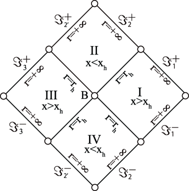
Figure 1: A black-bounce spacetime as a maximal extension of the asymptotically S-T Gamboa solution (4) for $\chi=\chi_{+}\in(\chi_{0},0)$ with $M=M_{+}(<0)$ and $h_{1}>0$ beyond the Killing horizon $x=x_{\rm h}$ under the assumption $\chi=\chi_{+}$ in the extended domain $x<x_{\rm h}$. The extended dynamical domain $x<x_{\rm h}$ is described by the Gamboa solution in the form of Eq. (4) with $M=M_{-}>0$. $\Im^{+(-)}$ stands for a future (past) null infinity and subscripts are to distinguish different null infinities.

Figure 2: A black-hole spacetime as a maximal extension of the asymptotically S-T Gamboa solution (4) for $\chi=\chi_{+}\in(\chi_{0},0)$ with $M=M_{+}(<0)$ and $h_{1}>0$ beyond the Killing horizon $x=x_{\rm h}$ under the assumption $\chi=\chi_{+}$ in the extended domain $x<x_{\rm h}$. The extended dynamical domain $x<x_{\rm h}$ is described by the Gamboa solution in the form of Eq. (17) with ${\bar{M}}={\bar{M}}_{-}<0$. A zigzag line corresponds to a curvature singularity located at $r=0$ corresponding to $x=x_{\rm s}(<x_{\rm h})$.

In fact, by Proposition 1, regions I–IV in Fig. 1 and Fig. 2 can be described by the Gamboa solution for different values of $\chi$ unless $\chi\in(\chi_{0},0)$ is satisfied. (See also Proposition 6 in Ref. addendum .) Even in such configurations, the bifurcation $(n-2)$-surface, denoted by B, is regular as shown in Appendix B. A physical explanation of this counterintuitive regularity was provided in Ref. Maeda:2024tpl based on the fact that the matter field in the dynamical region can be interpreted as a spacelike (tachyonic) perfect fluid. A fluid element of such a fluid in regions II and IV moves in a spacelike direction and does not cross neither a Killing horizon nor a bifurcation surface. Because orbits of the fluid elements do not have a past or future endpoint at B, the bifurcation $(n-2)$-surface B can be regular.

V Summary

In the present paper, we have investigated the Gamboa solution given in the form of Eq. (4) or (17) in general relativity, which is an exact two-parameter family of plane symmetric solutions admitting a hypersurface-orthogonal Killing vector $\xi^{\mu}\partial_{\mu}=\partial_{T}$ with a perfect fluid obeying an equation of state $p=\chi\rho$ in $n(\geq 4)$ dimensions GamboaSaravi . Proposition 1 is one of our main results that identifies all possible regular attachments of two Gamboa solutions for $\chi\in[-1/3,0)$, or equivalently $\beta\in[0,\infty)$, at the Killing horizon $x=x_{\rm h}$ in the regular coordinate system (35). We have also derived the conditions for the $C^{\infty}$ attachment at the horizon.

The other main result is that we have clarified the maximally extended spacetimes of the asymptotically topological S-T Gamboa solution (4) with $M=M_{+}<0$ and $h_{1}>0$ for $\chi\in(\chi_{0},0)$, or equivalently $\beta\in(2/(n-3),\infty)$, under the assumption that the value of $\chi$ is unchanged in the extended dynamical region. This result is summarized in Table 4. In more detail, we have shown the following.

1. For any value of $\chi\in(\chi_{0},0)$, the maximally extended spacetime describes (i) a globally regular and asymptotically topological S-T black bounce with a non-degenerate Killing horizon which coincides with a bounce null hypersurface, or (ii) an asymptotically topological S-T black hole with a non-degenerate Killing horizon and a spacelike curvature singularity inside the horizon.

2. In the black-bounce case, the metric in the single-null coordinates (35) is $C^{\infty}$ only for $\chi=-1/(1+2N)$ with odd $N$ satisfying $N>(n-1)/(n-3)$, and if the parameter in the extended region is given by $M=-M_{+}(>0)$.

3. In the black-hole case, the metric in the single-null coordinates (35) is $C^{\infty}$ only for odd $\beta$, or equivalently $\chi=-1/(1+2N)$ with even $N$ satisfying $N>(n-1)/(n-3)$, and if the parameter in the extended region is given by ${\bar{M}}=M_{+}(<0)$.

Because the NEC is violated away from the Killing horizon, our black bounce spacetime is expected to be dynamically unstable. Nevertheless, it is intriguing that such a configuration is possible as a plane symmetric solution because the vacuum solution does not describe a black hole unless a negative cosmological constant is introduced. Of course, it would be even more interesting if such a configuration were possible as an asymptotically flat spherically symmetric solution with a perfect fluid. This problem is left for future investigations.

Appendix A General static solution with $p=\chi\rho$ and a Ricci-flat base manifold.

In this appendix, we derive the most general $n(\geq 4)$-dimensional static solution with an $(n-2)$-dimensional Ricci-flat base manifold $K^{n-2}$ in general relativity with a perfect fluid (1) obeying a linear equation of state $p=\chi\rho$. In this system, without loss of generality, one may adopt the comoving coordinates with the radial coordinate $r$ as the areal radius such that

$$\begin{aligned} &{\rm d}s^{2}=-A(r){\rm d}T^{2}+B(r){\rm d}r^{2}+r^{2}\gamma_{ij}(z){\rm d}z^{i}{\rm d}z^{j},\\ &u^{\mu}\frac{\partial}{\partial x^{\mu}}=\frac{1}{\sqrt{A}}\frac{\partial}{\partial T},\end{aligned}$$ (84)

where $i,j=2,3,\cdots,n-1$ and $\gamma_{ij}$ is the metric on $K^{n-2}$. This problem was addressed in Ref. GamboaSaravi using the comoving coordinates but with a non-areal radial coordinate and assuming the $(n-2)$-dimensional flat base manifold $\mathbb{R}^{n-2}$. The generalization including a Ricci-flat base manifold is straightforward since the Einstein equations only require the Ricci tensor of $K^{n-2}$, which is null in the present case. However, the symmetries and global geometric properties of the spacetime can drastically differ after changing the base manifold.

In the coordinate system (84), the Einstein equations (1) are written as

$$\kappa_{n}\rho= \frac{n-2}{2r^{2}B}\left\{\frac{rB^{\prime}}{B}-(n-3)\right\},$$ (85)

$$\kappa_{n}p= \frac{n-2}{2r^{2}B}\left\{\frac{rA^{\prime}}{A}+(n-3)\right\},$$ (86)

$$\kappa_{n}p= \frac{1}{2r^{2}B}\biggl{[}-\frac{rB^{\prime}}{2B}\left\{\frac{rA^{\prime}}{A}+2(n-3)\right\}+\frac{r^{2}A^{\prime\prime}}{A}$$

$$+(n-3)\frac{rA^{\prime}}{A}-\frac{r^{2}{A^{\prime}}^{2}}{2A^{2}}+(n-3)(n-4)\biggl{]}.$$ (87)

The energy-momentum conservation equations $\nabla_{\nu}T^{\mu\nu}=0$ give

$$p^{\prime}=-\frac{A^{\prime}}{2A}(\rho+p).$$ (88)

Now we assume the linear equation of state $p=\chi\rho$. The dust case ($\chi=0$) is excluded from our consideration because Eq. (88) shows that $A$ is constant and it contradicts to Eq. (86) for $n\geq 4$, so that there is no static dust solution. In addition, Eq. (88) shows that a perfect fluid with $\chi=-1$ is equivalent to a cosmological constant $\Lambda$. Hence, by Birkhoff’s theorem with $\Lambda$, the general solution is identical to the topological Schwarzschild-Tangherlini-(anti-)de Sitter solution.

With $p=\chi\rho$ and $\chi\neq 0$, Eq. (88) is integrated yielding

$$\rho=c_{0}A^{-(1+\chi)/(2\chi)},$$ (89)

where $c_{0}$ is a constant. Moreover, Eqs. (85) and (86) leads to

$$\chi\frac{rB^{\prime}}{B}=\frac{rA^{\prime}}{A}+(n-3)(\chi+1),$$ (90)

which is easily integrated as

$$B= B_{0}r^{(n-3)(\chi+1)/\chi}A^{1/\chi},$$ (91)

where $B_{0}$ is an integration constant. In addition, Eq. (86) provides the following expression for $\rho$:

$$\rho= \frac{n-2}{2\chi\kappa_{n}B_{0}r^{[(n-1)\chi+(n-3)]/\chi}A^{1/\chi}}\left\{\frac{rA^{\prime}}{A}+(n-3)\right\}.$$ (92)

Introducing a new variable $a(r)$ such that

$$A(r)=r^{-(n-3)}a(r),$$ (93)

we obtain from Eqs. (91) and (92)

$$B= B_{0}r^{n-3}a^{1/\chi},$$ (94)

$$\rho= \frac{(n-2)a^{\prime}}{2\chi\kappa_{n}B_{0}r^{n-2}a^{(1+\chi)/\chi}},$$ (95)

respectively. Then, the comparison of Eqs. (89) and (95) yields the first-order differential equation

$$\begin{aligned} (n-2)a^{\prime}=&2\chi\kappa_{n}c_{0}B_{0}r^{(\zeta-2\chi)/(2\chi)}a^{(1+\chi)/(2\chi)},\\ \zeta:=&(3n-5)\chi+(n-3),\end{aligned}$$ (96)

which can be directly integrated by quadrature. The general solution to Eq. (96) is

$$a(r)=\left\{\begin{array}[]{ll}h^{-2\chi/(1-\chi)}&[\chi\neq 0,1]\\ \exp(A_{0}+A_{1}r^{2(n-2)})&[\chi=1]\end{array}\right.,$$ (99)

where $h(r)$ is defined by

$$\begin{aligned} h(r):=&\left\{\begin{array}[]{ll}A_{0}+A_{1}r^{\zeta/(2\chi)}&[\chi\neq\chi_{0}]\\ A_{0}+A_{1}\ln|r|&[\chi=\chi_{0}]\end{array}\right.,\\ \chi_{0}:=&-\frac{n-3}{3n-5}.\end{aligned}$$ (100)

Here $A_{0}$ is an integration constant and the constant $A_{1}$ is given by

$$A_{1}=\left\{\begin{array}[]{ll}-2\kappa_{n}c_{0}B_{0}\chi(1-\chi)/[(n-2)\zeta]&[\chi\neq 0,1,\chi_{0}]\\ -4\kappa_{n}c_{0}B_{0}/(3n-5)&[\chi=\chi_{0}]\\ \kappa_{n}c_{0}B_{0}/(n-2)^{2}&[\chi=1]\end{array}\right..$$ (104)

Although four integration constants appear in the general solution, the relation (104) reduces this number to three. In addition, the field equations (85)–(88) are clearly invariant under a constant rescaling of the lapse function $A(r)$, which is equivalent to a rescaling of the time coordinate $T$. Thus, another constant can be fixed without loss of generality. Therefore, the general solution is characterized by two parameters. One of these two parameters is associated with the conserved charge, the mass, corresponding to the time translation invariance of a static configuration, and the other is associated with the presence of a matter field.

Lastly, we give a brief comment on the case $\chi=1$. By means of a rescaling of $T$ and a redefinition of the integration constants, a suitable form of the general solution for $\chi=1$ is given by

$$\begin{aligned} {\rm d}s^{2}=&-{B}_{0}^{-1}r^{-(n-3)}\exp(A_{1}r^{2(n-2)}){\rm d}T^{2}\\ &+{B}_{0}r^{n-3}\exp(A_{1}r^{2(n-2)}){\rm d}r^{2}+r^{2}\gamma_{ij}{\rm d}z^{i}{\rm d}z^{j},\\ \rho&=p=\frac{(n-2)^{2}A_{1}r^{n-3}}{\kappa_{n}{B}_{0}\exp(A_{1}r^{2(n-2)})}.\end{aligned}$$ (105)

The solution (105) with $A_{1}=0$ is identical to the topological Schwarzschild-Tangherlini vacuum solution. In four dimensions ($n=4$), and when the base manifold is chosen as $\mathbb{R}^{2}$, this solution reproduces the static plane symmetric one obtained in Ref. Tabensky-Taub1973 .

Appendix B Regularity of the bifurcation $(n-2)$-surface

In this appendix, we show the regularity of the bifurcation $(n-2)$-surface, denoted by B in Fig. 1 and Fig. 2. For static and plane symmetric solutions with $\chi\in[-1/3,0)$, the asymptotic behaviors of the metric functions near a non-degenerate Killing horizon $x=x_{\rm h}$ in the domain $x>x_{\rm h}$ are given by Eq. (64). Now we write the metric near $x=x_{\rm h}$ in the domain $x>x_{\rm h}$ as

$$\begin{aligned} &H(x)\simeq H_{1}\Delta+H_{3+\beta}^{+}\Delta^{3+\beta},\\ &r(x)\simeq r_{\rm h}+r_{2+\beta}^{+}\Delta^{2+\beta},\end{aligned}$$ (106)

and in the domain $x<x_{\rm h}$ as

$$\begin{aligned} &H(x)\simeq H_{1}\Delta+H_{3+\beta}^{-}(-\Delta)^{3+\beta},\\ &r(x)\simeq r_{\rm h}+r_{2+\beta}^{-}(-\Delta)^{2+\beta},\end{aligned}$$ (107)

where $\Delta:=x-x_{\rm h}$ and $\beta\in[0,\infty)$ is defined by Eq. (8). Here $H_{1}$ and $r_{\rm h}$ are non-zero in particular. Although the values of the coefficients of the higher-order terms are different in general, the Killing horizon $x=x_{\rm h}$ is regular as the metric in the single-null coordinates (30) is at least $C^{1,1}$ there.

Using the tortoise coordinate $x_{*}:=\int H(x)^{-1}{\rm d}x$, we define the null Kruskal-Szekeres coordinates $U$ and $V$ by

$$U:=\mp e^{-H_{1}u/2},\qquad V:=e^{H_{1}v/2},$$ (108)

where $u:=t-x_{*}$ and $v:=t+x_{*}$. For a non-degenerate outer Killing horizon, characterized by $H_{1}>0$, $x=x_{\rm h}$ corresponds to $x_{*}\to-\infty$ and $UV=0$. The upper (lower) sign in the definition of $U$ in Eq. (108) corresponds to $x>(<)x_{\rm h}$. Then, the metric (30) in the quasi-global coordinates is written in the null Kruskal-Szekeres coordinates as

$$\begin{aligned} &{\rm d}s^{2}=2g_{UV}{\rm d}U{\rm d}V+r(x(U,V))^{2}{\rm d}l_{n-2}^{2},\\ &g_{UV}=\frac{2H(x(U,V))}{H_{1}^{2}UV}.\end{aligned}$$ (109)

With both Eqs. (106) and (107), the asymptotic behaviors of the metric functions near a Killing horizon $x_{*}\to-\infty$ ($UV=0$) are given by

$$\begin{aligned} g_{UV}\simeq&\frac{2}{H_{1}^{2}}\biggl{(}-1+O(U^{3}V^{3})\biggl{)},\\ r^{2}\simeq&r_{\rm h}^{2}+O(U^{2}V^{2}).\end{aligned}$$ (110)

Equation (110) shows that the metric is at least $C^{1,1}$ and hence regular also at a bifurcation $(n-2)$-surface given by $U=V=0$.

Appendix C Matter field on the Killing horizon for $\chi=-1/3$

In this appendix, we derive an explicit form of the matter field confined on the Killing horizon $x=x_{\rm h}$ in the Gamboa solution for $\chi=-1/3$. For $\chi=-1/3$, the matter field at $x=x_{\rm h}$ is a null dust fluid by Proposition 2 and Corollary 1 in Ref. Maeda:2021ukk . Using Eq. (72) with $\chi=-1/3$ ($\beta=0$), we obtain its energy-momentum tensor as

$$T_{\mu\nu}|_{x=x_{\rm h}}=\sigma k_{\mu}k_{\nu},\qquad k^{\mu}\frac{\partial}{\partial x^{\mu}}={\cal K}\frac{\partial}{\partial v},$$ (111)

where $\sigma$ is the energy density of the null dust and $k^{\mu}$ is a null vector satisfying $k_{\mu}k^{\mu}=0$ and

$$\sigma{\cal K}^{2}= -\frac{(n-2)r^{\prime\prime}}{\kappa_{n}r}\biggl{|}_{x=x_{\rm h}}=-\frac{4(n-2)M^{2}}{\kappa_{n}r_{\rm h}^{4}}.$$ (112)

Since $\sigma<0$ is satisfied, the null dust confined on the Killing horizon violates all the standard energy conditions. (See section 4.2 in Ref. Maeda:2018hqu .) The tangent vector $k^{\mu}$ is arbitrary to multiply by a scalar function because it is null. As a natural choice, we choose $k^{\mu}$ as a null generator of the Killing horizon.

Consider an affinely parametrized future-directed radial null geodesic $\gamma$ in the spacetime described by the metric in the single-null coordinates (35). The orbit of $\gamma$ is given by $x^{\mu}=(v(\lambda),x(\lambda),0,\cdots,0)$ with its tangent vector $k^{\mu}=({\dot{v}},{\dot{x}},0,\cdots,0)$, where $\lambda$ is an affine parameter along $\gamma$ and a dot denotes differentiation with respect to $\lambda$. Then, null geodesic equations $k^{\nu}\nabla_{\nu}k^{\mu}=0$ for $\gamma$ are written as

$$0= {\ddot{v}}+\frac{1}{2}H^{\prime}{\dot{v}}^{2},$$ (113)

$$0= {\ddot{x}}+\frac{1}{2}HH^{\prime}{\dot{v}}^{2}-H^{\prime}{\dot{v}}{\dot{x}},$$ (114)

which admit the following solution

$$v(\lambda)= r_{\rm h}^{n-3}\ln|\lambda-\lambda_{0}|+v_{0},\qquad x(\lambda)=x_{\rm h},$$ (115)

where we have used $H(x_{\rm h})=0$ and $H^{\prime}(x_{\rm h})=2/r_{\rm h}^{n-3}$ given by Eq. (72) and $v_{0}$ and $\lambda_{0}$ are integration constants.

The solution (115) is a null generator of the Killing horizon $x=x_{\rm h}$ and $\lambda\to\lambda_{0}$ corresponds to a bifurcation $(n-2)$-surface $v\to-\infty$, on which the Killing vector generating staticity vanishes. Identifying the solution (115) as the orbit of a null dust fluid on the Killing horizon (111), we obtain $\sigma$ and ${\cal K}$ as

$$\sigma=-\frac{4(n-2)M^{2}}{\kappa_{n}r_{\rm h}^{2(n-1)}}(\lambda-\lambda_{0})^{2},\qquad{\cal K}=\frac{r_{\rm h}^{n-3}}{\lambda-\lambda_{0}}.$$ (116)

The energy density $\sigma$ converges to zero in the limit to a bifurcation $(n-2)$-surface $\lambda\to\lambda_{0}$.

References

- (1) H. Maeda, “Quest for realistic non-singular black-hole geometries: regular-center type”, JHEP 11 (2022), 108 doi:10.1007/JHEP11(2022)108 [arXiv:2107.04791 [gr-qc]].
- (2) J.M. Bardeen, in Proceedings of International Conference GR5 (Tbilisi, USSR, 1968) p. 174.
- (3) S. A. Hayward, “Formation and evaporation of regular black holes”, Phys. Rev. Lett. 96, 031103 (2006) doi:10.1103/PhysRevLett.96.031103 [arXiv:gr-qc/0506126 [gr-qc]].
- (4) I. Dymnikova, “Regular electrically charged structures in nonlinear electrodynamics coupled to general relativity”, Class. Quant. Grav. 21 (2004), 4417-4429 doi:10.1088/0264-9381/21/18/009 [arXiv:gr-qc/0407072 [gr-qc]].
- (5) Z. Y. Fan and X. Wang, “Construction of Regular Black Holes in General Relativity”, Phys. Rev. D 94 (2016) no.12, 124027 doi:10.1103/PhysRevD.94.124027 [arXiv:1610.02636 [gr-qc]].
- (6) E. Ayón-Beato and A. García, “The Bardeen model as a nonlinear magnetic monopole”, Phys. Lett. B 493, 149-152 (2000) doi:10.1016/S0370-2693(00)01125-4 [arXiv:gr-qc/0009077 [gr-qc]].
- (7) S. Chinaglia and S. Zerbini, “A note on singular and non-singular black holes”, Gen. Rel. Grav. 49 (2017) no.6, 75 doi:10.1007/s10714-017-2235-6 [arXiv:1704.08516 [gr-qc]].
- (8) P. A. Cano and Á. Murcia, “Resolution of Reissner-Nordström singularities by higher-derivative corrections”, Class. Quant. Grav. 38 (2021) no.7, 075014 doi:10.1088/1361-6382/abd923 [arXiv:2006.15149 [hep-th]].
- (9) P. Bueno, P. A. Cano and R. A. Hennigar, “Regular black holes from pure gravity”, Phys. Lett. B 861, 139260 (2025) doi:10.1016/j.physletb.2025.139260 [arXiv:2403.04827 [gr-qc]].
- (10) K. A. Bronnikov, V. N. Melnikov and H. Dehnen, “Regular black holes and black universes”, Gen. Rel. Grav. 39 (2007), 973-987 doi:10.1007/s10714-007-0430-6 [arXiv:gr-qc/0611022 [gr-qc]].
- (11) A. Simpson and M. Visser, “Black-bounce to traversable wormhole”, JCAP 02 (2019), 042 doi:10.1088/1475-7516/2019/02/042 [arXiv:1812.07114 [gr-qc]].
- (12) E. Poisson and W. Israel, “Inner-horizon instability and mass inflation in black holes”, Phys. Rev. Lett. 63, 1663-1666 (1989) doi:10.1103/PhysRevLett.63.1663
- (13) E. Poisson and W. Israel, “Internal structure of black holes”, Phys. Rev. D 41, 1796-1809 (1990) doi:10.1103/PhysRevD.41.1796
- (14) A. Ori, “Inner structure of a charged black hole: An exact mass-inflation solution”, Phys. Rev. Lett. 67, 789-792 (1991) doi:10.1103/PhysRevLett.67.789
- (15) A. Bonanno, A. P. Khosravi and F. Saueressig, “Regular black holes with stable cores”, Phys. Rev. D 103, no.12, 124027 (2021) doi:10.1103/PhysRevD.103.124027 [arXiv:2010.04226 [gr-qc]].
- (16) R. Carballo-Rubio, F. Di Filippo, S. Liberati, C. Pacilio and M. Visser, “Inner horizon instability and the unstable cores of regular black holes”, JHEP 05, 132 (2021) doi:10.1007/JHEP05(2021)132 [arXiv:2101.05006 [gr-qc]].
- (17) F. Di Filippo, R. Carballo-Rubio, S. Liberati, C. Pacilio and M. Visser, “On the Inner Horizon Instability of Non-Singular Black Holes”, Universe 8 (2022) no.4, 204 doi:10.3390/universe8040204 [arXiv:2203.14516 [gr-qc]].
- (18) R. Carballo-Rubio, F. Di Filippo, S. Liberati, C. Pacilio and M. Visser, “Regular black holes without mass inflation instability”, JHEP 09 (2022), 118 doi:10.1007/JHEP09(2022)118 [arXiv:2205.13556 [gr-qc]].
- (19) R. Carballo-Rubio, F. Di Filippo, S. Liberati and M. Visser, “Mass Inflation without Cauchy Horizons”, Phys. Rev. Lett. 133, no.18, 181402 (2024) doi:10.1103/PhysRevLett.133.181402 [arXiv:2402.14913 [gr-qc]].
- (20) K. A. Bronnikov and J. C. Fabris, “Regular phantom black holes”, Phys. Rev. Lett. 96, 251101 (2006) doi:10.1103/PhysRevLett.96.251101 [arXiv:gr-qc/0511109 [gr-qc]].
- (21) S. V. Bolokhov, K. A. Bronnikov and M. V. Skvortsova, “Magnetic black universes and wormholes with a phantom scalar”, Class. Quant. Grav. 29 (2012), 245006 doi:10.1088/0264-9381/29/24/245006 [arXiv:1208.4619 [gr-qc]].
- (22) K. A. Bronnikov, K. Badalov and R. Ibadov, “Arbitrary Static, Spherically Symmetric Space-Times as Solutions of Scalar-Tensor Gravity”, Grav. Cosmol. 29 (2023) no.1, 43-49 doi:10.1134/S0202289323010036 [arXiv:2212.04544 [gr-qc]].
- (23) J. Barrientos, A. Cisterna, N. Mora and A. Viganò, “AdS-Taub-NUT spacetimes and exact black bounces with scalar hair”, Phys. Rev. D 106 (2022) no.2, 024038 doi:10.1103/PhysRevD.106.024038 [arXiv:2202.06706 [hep-th]].
- (24) P. Cañate, “Black bounces as magnetically charged phantom regular black holes in Einstein-nonlinear electrodynamics gravity coupled to a self-interacting scalar field”, Phys. Rev. D 106 (2022) no.2, 024031 doi:10.1103/PhysRevD.106.024031 [arXiv:2202.02303 [gr-qc]].
- (25) K. A. Bronnikov, “Black bounces, wormholes, and partly phantom scalar fields”, Phys. Rev. D 106 (2022) no.6, 064029 doi:10.1103/PhysRevD.106.064029 [arXiv:2206.09227 [gr-qc]].
- (26) M. E. Rodrigues and M. V. d. S. Silva, “Source of black bounces in general relativity”, Phys. Rev. D 107 (2023) no.4, 044064 doi:10.1103/PhysRevD.107.044064 [arXiv:2302.10772 [gr-qc]].
- (27) K. A. Bronnikov, M. E. Rodrigues and M. V. de S. Silva, “Cylindrical black bounces and their field sources”, Phys. Rev. D 108 (2023) no.2, 024065 doi:10.1103/PhysRevD.108.024065 [arXiv:2305.19296 [gr-qc]].
- (28) G. Alencar, K. A. Bronnikov, M. E. Rodrigues, D. Sáez-Chillón Gómez and M. V. de S. Silva, “On black bounce space-times in non-linear electrodynamics”, Eur. Phys. J. C 84, no.7, 745 (2024) doi:10.1140/epjc/s10052-024-13119-4 [arXiv:2403.12897 [gr-qc]].
- (29) H. Huang and J. Yang, “Charged Ellis Wormhole and Black Bounce”, Phys. Rev. D 100, no.12, 124063 (2019) doi:10.1103/PhysRevD.100.124063 [arXiv:1909.04603 [gr-qc]].
- (30) J. Yang and H. Huang, “Trapping horizons of the evolving charged wormhole and black bounce”, Phys. Rev. D 104, no.8, 084005 (2021) doi:10.1103/PhysRevD.104.084005 [arXiv:2104.11134 [gr-qc]].
- (31) C. F. S. Pereira, D. C. Rodrigues, J. C. Fabris and M. E. Rodrigues, “Black-bounce solution in k-essence theories”, Phys. Rev. D 109 (2024) no.4, 044011 doi:10.1103/PhysRevD.109.044011 [arXiv:2309.10963 [gr-qc]].
- (32) C. F. S. Pereira, D. C. Rodrigues, É. L. Martins, J. C. Fabris and M. E. Rodrigues, “New sources of ghost fields in k-essence theories for black-bounce solutions”, Class. Quant. Grav. 42, no.1, 015001 (2025) doi:10.1088/1361-6382/ad98e0 [arXiv:2405.07455 [gr-qc]].
- (33) C. F. S. Pereira, D. C. Rodrigues, M. V. d. S. Silva, J. C. Fabris, M. E. Rodrigues and H. Belich, “Magnetically charged black-bounce solution via nonlinear electrodynamics in a k-essence theory”, Phys. Rev. D 111, no.8, 084025 (2025) doi:10.1103/PhysRevD.111.084025 [arXiv:2409.09182 [gr-qc]].
- (34) F. S. N. Lobo, M. E. Rodrigues, M. V. de Sousa Silva, A. Simpson and M. Visser, “Novel black-bounce spacetimes: wormholes, regularity, energy conditions, and causal structure”, Phys. Rev. D 103, no.8, 084052 (2021) doi:10.1103/PhysRevD.103.084052 [arXiv:2009.12057 [gr-qc]].
- (35) E. Franzin, S. Liberati, J. Mazza, A. Simpson and M. Visser, “Charged black-bounce spacetimes”, JCAP 07, 036 (2021) doi:10.1088/1475-7516/2021/07/036 [arXiv:2104.11376 [gr-qc]].
- (36) K. A. Bronnikov and R. K. Walia, “Field sources for Simpson-Visser spacetimes”, Phys. Rev. D 105, no.4, 044039 (2022) doi:10.1103/PhysRevD.105.044039 [arXiv:2112.13198 [gr-qc]].
- (37) L. A. Lessa and G. J. Olmo, “On the structure of black bounces sourced by anisotropic fluids”, JCAP 03, 019 (2025) doi:10.1088/1475-7516/2025/03/019 [arXiv:2412.05378 [gr-qc]].
- (38) E. L. B. Junior and M. E. Rodrigues, “Black-bounce in f(T) gravity”, Gen. Rel. Grav. 55, no.1, 8 (2023) doi:10.1007/s10714-022-03048-6 [arXiv:2203.03629 [gr-qc]].
- (39) J. C. Fabris, E. L. B. Junior and M. E. Rodrigues, “Generalized models for black-bounce solutions in f(R) gravity”, Eur. Phys. J. C 83, no.10, 884 (2023) doi:10.1140/epjc/s10052-023-12022-8 [arXiv:2310.00714 [gr-qc]].
- (40) J. T. S. S. Junior, F. S. N. Lobo and M. E. Rodrigues, “Black bounces in conformal Killing gravity”, Eur. Phys. J. C 84, no.6, 557 (2024) doi:10.1140/epjc/s10052-024-12922-3 [arXiv:2405.09702 [gr-qc]].
- (41) E. L. B. Junior, J. T. S. S. Junior, F. S. N. Lobo, M. E. Rodrigues, D. Rubiera-Garcia, L. F. D. da Silva and H. A. Vieira, “Black bounces in Cotton gravity”, Eur. Phys. J. C 84, no.11, 1190 (2024) doi:10.1140/epjc/s10052-024-13568-x [arXiv:2407.21649 [gr-qc]].
- (42) J. Furtado and G. Alencar, “BTZ Black-Bounce to Traversable Wormhole”, Universe 8, no.12, 625 (2022) doi:10.3390/universe8120625 [arXiv:2210.06608 [gr-qc]].
- (43) M. S. Churilova and Z. Stuchlik, “Ringing of the regular black-hole/wormhole transition”, Class. Quant. Grav. 37, no.7, 075014 (2020) doi:10.1088/1361-6382/ab7717 [arXiv:1911.11823 [gr-qc]].
- (44) E. Franzin, S. Liberati, J. Mazza, R. Dey and S. Chakraborty, “Scalar perturbations around rotating regular black holes and wormholes: Quasinormal modes, ergoregion instability, and superradiance”, Phys. Rev. D 105, no.12, 124051 (2022) doi:10.1103/PhysRevD.105.124051 [arXiv:2201.01650 [gr-qc]].
- (45) S. R. Wu, B. Q. Wang, D. Liu and Z. W. Long, “Echoes of charged black-bounce spacetimes”, Eur. Phys. J. C 82, no.11, 998 (2022) doi:10.1140/epjc/s10052-022-10938-1 [arXiv:2201.08415 [gr-qc]].
- (46) M. Guerrero, G. J. Olmo, D. Rubiera-Garcia and D. S. C. Gómez, “Shadows and optical appearance of black bounces illuminated by a thin accretion disk”, JCAP 08, 036 (2021) doi:10.1088/1475-7516/2021/08/036 [arXiv:2105.15073 [gr-qc]].
- (47) Y. Guo and Y. G. Miao, “Charged black-bounce spacetimes: Photon rings, shadows and observational appearances”, Nucl. Phys. B 983, 115938 (2022) doi:10.1016/j.nuclphysb.2022.115938 [arXiv:2112.01747 [gr-qc]].
- (48) H. C. D. Lima, Junior., L. C. B. Crispino, P. V. P. Cunha and C. A. R. Herdeiro, “Can different black holes cast the same shadow?”, Phys. Rev. D 103, no.8, 084040 (2021) doi:10.1103/PhysRevD.103.084040 [arXiv:2102.07034 [gr-qc]].
- (49) J. R. Nascimento, A. Y. Petrov, P. J. Porfirio and A. R. Soares, “Gravitational lensing in black-bounce spacetimes”, Phys. Rev. D 102, no.4, 044021 (2020) doi:10.1103/PhysRevD.102.044021 [arXiv:2005.13096 [gr-qc]].
- (50) N. Tsukamoto, “Gravitational lensing in the Simpson-Visser black-bounce spacetime in a strong deflection limit”, Phys. Rev. D 103, no.2, 024033 (2021) doi:10.1103/PhysRevD.103.024033 [arXiv:2011.03932 [gr-qc]].
- (51) S. U. Islam, J. Kumar and S. G. Ghosh, “Strong gravitational lensing by rotating Simpson-Visser black holes”, JCAP 10, 013 (2021) doi:10.1088/1475-7516/2021/10/013 [arXiv:2104.00696 [gr-qc]].
- (52) N. Tsukamoto, “Gravitational lensing by two photon spheres in a black-bounce spacetime in strong deflection limits”, Phys. Rev. D 104, no.6, 064022 (2021) doi:10.1103/PhysRevD.104.064022 [arXiv:2105.14336 [gr-qc]].
- (53) X. T. Cheng and Y. Xie, “Probing a black-bounce, traversable wormhole with weak deflection gravitational lensing”, Phys. Rev. D 103, no.6, 064040 (2021) doi:10.1103/PhysRevD.103.064040
- (54) R. E. Gamboa Saraví, “Higher-dimensional perfect fluids and empty singular boundaries”, Gen. Rel. Grav. 44, 1769-1786 (2012) doi:10.1007/s10714-012-1366-z [arXiv:1204.4907 [gr-qc]].
- (55) H. Maeda, “Fake Schwarzschild and Kerr black holes”, [arXiv:2410.11937 [gr-qc]].
- (56) H. Maeda and C. Martínez, “Energy conditions in arbitrary dimensions”, PTEP 2020 (2020) no.4, 4 doi:10.1093/ptep/ptaa009 [arXiv:1810.02487 [gr-qc]].
- (57) H. Maeda and C. Martínez, “Existence and absence of Killing horizons in static solutions with symmetries”, Class. Quant. Grav. 41, no.24, 245013 (2024) doi:10.1088/1361-6382/ad8ea4 [arXiv:2402.11012 [gr-qc]].
- (58) H. Maeda, “Hawking-Ellis type of matter on Killing horizons in symmetric spacetimes”, Phys. Rev. D 104 (2021) no.8, 8 doi:10.1103/PhysRevD.104.084088 [arXiv:2107.01455 [gr-qc]].
- (59) H. Maeda and C. Martínez, “Planar black holes and black bounces with flat exterior”, [arXiv:2506.11184 [gr-qc]].
- (60) H. Maeda and C. Martínez, “Addendum: Existence and absence of Killing horizons in static solutions with symmetries (2024 Class. Quantum Grav. 41, 245013)”, doi:10.1088/1361-6382/ade35a
- (61) R. Tabensky and A. H. Taub, “Plane symmetric self-gravitating fluids with pressure equal to energy density”, Comm. Math. Phys. 29 (1973), 61 doi.org/10.1007/BF01661153