Black holes in $f(R,T)$ gravity coupled with Euler-Heisenberg electrodynamics

Abstract

We investigate the scenario of black holes coupled with the Euler-Heisenberg nonlinear electromagnetic field in the framework of $f(R,T)$ gravity. The black hole solutions for electrically charged, magnetically charged and the dyonic case are separately analyzed, and we discuss the scalar curvature and the energy conditions of the black hole spacetime. In the magnetic charge solution, the $f(R,T)$ correction appears in the $1/r^{6}$ Euler-Heisenberg electromagnetic field correction term, while the electrically charged solution includes an $r^{2}$ term, with the curvature of the spacetime determined by the $f(R,T)$ coupling parameter. The dyonic solution is obtained through vacuum polarization quantum electrodynamics corrections, where electromagnetic duality is broken and the solution exists higher-order correction terms. The relationship between the event horizon and charge of dyonic extreme black holes is studied. Furthermore, we investigate the effective metric, photon trajectories, and innermost stable circular orbit under nonlinear electromagnetic effects, providing images of photon geodesic for varying electric and magnetic charge strengths and $f(R,T)$ coupling parameter.

I Introduction

Einstein’s General Relativity (GR), as the cornerstone of modern gravitational physics, successfully predict many physical phenomena [1, 2, 3]. In recent years, due to advanced observational precision, GR has encountered difficulties in explaining phenomena such as the accelerated expansion of the universe [4, 5, 6, 7], dark energy and dark matter [8, 9, 10, 5, 11], making the development of new theories to better describe the cosmology. The $f(R,T)$ gravity theory can be regarded as the maximal extension of the Hilbert-Einstein action and has been widely applied in cosmological studies, particularly addressing the issues of early universe inflation and late-time accelerated expansion. Compared to the $f(R)$ gravity (see Refs. [12, 13, 14] for a review), the $f(R,T)$ gravity introduces a direct coupling between matter and geometry. This coupling allows the matter field to directly influence the evolution of geometry. Specific functional forms of $f(R,T)$ have been used to fit observational data, such as Type Ia supernova data [15, 16, 17] and cosmic microwave background(CMB) radiation [18]. Related studies include energy condition analyses [19], investigations of white dwarfs and exotic stars [20, 21, 22, 23]. In the field of quantum cosmology, $f(R,T)$ gravity has also been explored to study its quantum behavior under the Friedmann-Robertson-Walker metric [24, 25], aiming to explain the early evolution of the universe [26, 27], etc.

The motion of particles and fluids with pressure in the $f(R,T)$ gravity framework no longer follows geodesics but is influenced by an extra force. This prediction differs from the classical results of general relativity, may leading to orbit deviations in regions with high density gradients (e.g., the edges of galaxy clusters) [28, 29]. The extra force could account for small deviations in Mercury precession [30]. In a cosmological context, this force may affect the dynamics of cosmic expansion. Non-geodesic motion could modify the polarization modes or propagation speed of gravitational waves [31, 32]. Some studies suggest parameters are tightly constrained by Solar System test in the parameter-Post-Newtonian(PPN) formalism [30, 33]. In this paper, we will consider the minimal coupling model and constrain the parameters to slightly exceed the solar system PPN test.

The Euler-Heisenberg(EH) nonlinear electromagnetic field is considered as the matter section of the action to investigate the interaction between nonlinear electromagnetic fields and $f(R,T)$ gravity. In 1936, Euler and Heisenberg proposed a nonlinear electrodynamics based on Dirac theory [34], it is an effective theory derived from quantum electrodynamics (QED) after one-loop quantization. The vacuum is treated as a medium with a dielectric constant, with its polarizability and magnetizability described as a cloud of virtual charges surrounding real currents and charges. Schwinger reformulated this one-loop effective Lagrangian within the QED framework [35]. The static black hole solutions in the Einstein-Euler-Heisenberg (EEH) framework with electric, magnetic, and dyonic charges are investigated [36, 37, 38], and they treated as screened Reissner-Nordstr’́om (RN) solutions. Nonlinear effects play a role only in the screening of charges, generating virtual charges around real charges and currents. These effects introduce QED corrections to the black hole horizon, entropy, total energy, and maximum extractable energy [39, 40, 41, 42, 43, 44]. The EH effect is measurable [45, 46]. Experimentally, when the electromagnetic field strength is high, the EH theory provides a more accurate classical approximation of QED compared to Maxwell theory [47]. The EH action breaks electromagnetic duality at higher orders of the electromagnetic field, leading to significant distinctions in black hole solutions with electric or magnetic charges [48]. From a modern perspective, string theory and D-brane physics, in the low-energy limit, give rise to Abelian and non-Abelian Born-Infeld (BI) lagrangians [49, 50, 51]. Subsequent work has extensively studied the asymptotically flat, static, spherically symmetric black hole solutions of the Einstein-BI theory [52, 53]. As a low-energy limit of the BI theory, under appropriate parameters, the EH action effectively approximates the supersymmetric system of minimally coupled particles with spins -1/2 and 0 [54]. Ref. [55] constrains the nonlinear parameter $a>0$, relating it to the inverse string tension $\alpha^{\prime}$, and studies the effective EH Lagrangian as the low-energy limit of BI black hole solutions [56, 57, 58, 38, 59, 60, 61, 62, 63, 64, 65].

The two different interpretations of the EH theory lead to distinct choices of parameters in the Lagrangian. In the EH theory with QED corrections from vacuum polarization generating virtual charges, the parameters in the Lagrangian are considered very small values, which we will discuss in the context of dyonic black hole solutions. As the low-energy limit of the BI theory—where BI serves as the effective theory on string theory—the EH allows parameters to be interpreted as the inverse string tension $\alpha^{\prime}$ (a free parameter), which we will address in solutions for magnetic and electric charge black holes.

Utilizing Very-Long-Baseline Interferometry(VLBI), the Event Horizon Telescope (EHT) collaboration successfully obtained the high-resolution images of the supermassive black hole Sgr A* at our Galactic Center [66, 67, 68, 69, 70, 71]. The observation indicates that this black hole exhibits a ring-like structure analogous to the M87* black hole released in 2019 – featuring a central dark region encircled by a bright emission ring [72, 73, 74, 75, 76, 77]. General relativity predicts significant deflection of photons traversing strong gravitational fields: some photons are captured by the black hole, forming the shadow region, while some escapes and form photon rings around the black hole. This phenomenon provides a new sight for extreme gravitational environments [78]. Theoretical investigations of black hole shadows begins from Synge’s work on the Schwarzschild spacetime [79]. Bardeen et al. subsequently extended this research to the Kerr black hole scenario [80]. Luminet pioneered the numerical simulation of shadows for rotating black holes with accretion disks [81]. Contemporary theoretical models, incorporating radiated emissions from accreting matter, provide robust explanations for the EHT observations of both M87* and SgrA* [82, 83, 84]. Recent research has expanded into richer theoretical frameworks, including: Born-Infeld spacetimes [85, 86], perfect fluid dark matter models [87], Gauss-Bonnet AdS spacetimes [88], hairy Schwarzschild black holes [89], and black hole systems exhibiting multiple photon spheres [90, 91, 92, 93, 94, 95]. Black hole shadows offer insights into potential effects of modified gravity theories and cold dark matter in the early universe [96]. In this paper we will discuss the impacts of modified gravity and the nonlinear electrodynamics effect on photon orbits.

The structure of this paper is as follows: In Section II, we review $f(R,T)$ gravity theory, present the modified $f(R,T)$-EH action, and derive the field equations under minimum coupling $f(R,T)$. In Section III, we provide the black hole solution for the magnetic monopole EH field and discuss the nature of singularities. Section IV electrically charged black holes is considered. Both Section III and Section IV employ the Euler-Heisenberg interpretation of BI electrodynamics in low-energy limit. In Section V, we use the EH explanation based on vacuum charge polarization to analyze the dyonic black hole solution. In Section VI, energy conditions are qualitatively analyzed. In Section VII, we thoroughly investigate the effective metric, photon trajectories, and innermost stable circular orbit (ISCO) under nonlinear electromagnetic effects, providing images of photon geodesic integrals for varying electric and magnetic charge strengths and $f(R,T)$ coupling parameters. Finally, Section VIII summarizes the paper. For simplicity, we set the natural units $c=G_{n}=\hbar=1$ throughout the paper, and black hole mass is fixed at $M=1$.

II Field equations of $f(R,T)$ gravity coupled with EH electrodynamics

According to Ref. [97] and combining the EEH action [55], we assume the EH nonlinear electromagnetic field as the matter section in the action, and this gravitational system can be described as

$$S=\frac{1}{16\pi}\int f(R,T)\sqrt{-g}\,d^{4}x+\int\mathcal{L}(F)\sqrt{-g}\,d^{4}x\,,$$ (1)

where we have $g=\det(g_{\mu\nu})$, $f(R,T)$ is an arbitrary function of the scalar curvature $R$ and of the energy-momentum tensor trace $T$, $\mathcal{L}(F)$ is the Lagrangian density of EH field, which has the form [55, 98]

$$\mathcal{L}(F)=\frac{1}{4\pi}(-F+aF^{2}+bG^{2}),$$ (2)

the invariants are defined as $F\equiv\frac{1}{4}F^{\mu\nu}F_{\mu\nu}$, $G\equiv\frac{1}{4}F_{\mu\nu}*F^{\mu\nu}$, where the $*F^{\mu\nu}$ is the dual form of the electromagnetic strength tensor $F_{\mu\nu}$. The parameters $a,b$ are the coupling constants due to the weak field approximation and we have $a=he^{4}/(360\pi^{2}m_{e}^{4})\approx 0.001768,b=7he^{4}/(1440\pi^{2}m_{e}^{4})\approx 0.003095$, $h$ is the Plank constant, $e,m$ are the charge and the mass of electron, respectively [34]. For BI low energy limit, the EH allows parameters $a,b$ to be interpreted as the inverse string tension $\alpha^{\prime}$, which means they are free parameters. Varying this action with respect to $g^{\mu\nu}$ and gauge field $A_{\mu}$, we can obtain the equation of motion

$$\begin{split}\delta S=&\frac{1}{16\pi}\int\left[f_{R}(R,T)R_{\mu\nu}\delta g^{\mu\nu}+f_{R}(R,T)g_{\mu\nu}\Box\delta g^{\mu\nu}+\right.\\ &\left.-f_{R}(R,T)\nabla_{\mu}\nabla_{\nu}\delta g^{\mu\nu}+f_{T}(R,T)\frac{\delta(g^{\alpha\beta}T_{\alpha\beta})}{\delta g^{\mu\nu}}\delta g^{\mu\nu}+\right.\\ &\left.-\frac{1}{2}g_{\mu\nu}f(R,T)\delta g^{\mu\nu}+\frac{16\pi}{\sqrt{-g}}\frac{\delta(\sqrt{-g}\mathcal{L}_{D})}{\delta g^{\mu\nu}}\right]\sqrt{-g}d^{4}x,\end{split}$$ (3)

$$\frac{1}{\sqrt{-g}}\partial_{\mu}\left[\sqrt{-g}\left(2f_{T}(R,T)\mathcal{L}_{FF}F-\mathcal{L}_{F}\right)F^{\mu\nu}\right]=0,$$ (4)

where $\mathcal{L}_{F}=\partial\mathcal{L}/\partial F,\mathcal{L}_{FF}=\partial^{2}\mathcal{L}/\partial F^{2}$. Yields the modified Einstein field equation reads

$$G_{\mu\nu}\equiv f_{R}R_{\mu\nu}+\left(g_{\mu\nu}\Box-\nabla_{\mu}\nabla_{\nu}\right)f_{R}-\frac{1}{2}fg_{\mu\nu}=T_{\mu\nu}-f_{T}(T_{\mu\nu}+\Theta_{\mu\nu}),$$ (5)

here we have $f_{R}=\partial f/\partial R$, $f_{T}=\partial f/\partial T$ and$\Box=\nabla_{\rho}\nabla^{\rho}$. The energy-momentum tensor $T_{\mu\nu}$ and $\Theta_{\mu\nu}$ reads

$$T_{\mu\nu}\equiv-\frac{2}{\sqrt{-g}}\frac{\delta(\sqrt{-g}\mathcal{L}(F)}{\delta g^{\mu\nu}},$$ (6)

$$\Theta_{\mu\nu}\equiv g^{\alpha\beta}\frac{\delta T_{\alpha\beta}}{\delta g^{\mu\nu}}=-2T_{\mu\nu}+g_{\mu\nu}\mathcal{L}(F)-2g^{\alpha\beta}\frac{\partial^{2}\mathcal{L}(F)}{\partial g^{\mu\nu}g^{\alpha\beta}},$$ (7)

using the result mentioned in Ref. [99]

$$\delta\ln|\det-g|=-Tr(g^{\mu\nu}\delta g_{\mu\nu}),$$ (8)

then the Eq. (6) and Eq. (7) can be expressed as

$$\begin{split}T_{\mu\nu}&=g_{\mu\nu}\mathcal{L}(E)-\mathcal{L}_{F}F_{\mu\rho}F_{\nu}^{\rho},\\ \Theta_{\mu\nu}&=-g_{\mu\nu}\mathcal{L}(E)+\mathcal{L}_{F}F_{\mu\rho}F_{\nu}^{\rho}-2\mathcal{L}_{FF}FF_{\mu\rho}F_{\nu}^{\rho},\end{split}$$ (9)

taking the trace of the Einstein equation, we can derive

$$\Box f_{R}=\frac{1}{3}\left(T-f_{T}(T+\Theta)+2f-f_{R}R\right).$$ (10)

We choose the linear coupling form [97] $f(R,T)=R+2\beta T$, and the field equation can be expressed as

$$R_{\mu\nu}+\frac{1}{2}Rg_{\mu\nu}=8\pi T_{\mu\nu}-2\beta(T_{\mu\nu}+\Theta_{\mu\nu})+\beta Tg_{\mu\nu}.$$ (11)

Noticed that when $\beta=0$, it reduces to Einstein gravity. The product of the energy-momentum tensor trace $T$ and the metric $g_{\mu\nu}$ indicates that matter evolution affects spacetime geometry, similar to dark energy models, explaining cosmic acceleration. In the early universe, the evolution of $T$ under high-energy scales significantly alters the inflation [26]. This paper focuses on the spacetime structure coupled with the EH nonlinear electromagnetic field, discussed in detail in the following section.

III Magnetically charged black holes

The EH theory is a nonlinear electromagnetic theory, serves as an effective field theory of quantum electrodynamics (QED) in the low-energy limit and takes into account the nonlinear effects in strong electromagnetic fields. In Ref. [55], the EH parameter $a$ is treated as a strength of inverse string tension $\alpha^{\prime}$. Due to the definitions $\alpha$ is not a fixed constant. Under this framework, the magnetic monopole model introduces magnetic charges similar to Dirac magnetic monopoles [100], describing static, spherically symmetric black hole solutions. We have $Q_{e}\equiv 0$, and the gauge potential is $A_{\mu}=(0,0,0,Q_{m}\cos\theta)$. The nonzero components of $F_{\mu\nu}$ and the invariants $F,G$ are

$$F_{\theta\phi}=-F_{\phi\theta}=Q_{m}\sin\theta,\quad F=\frac{Q_{m}^{2}}{2r^{4}},\quad G=0.$$ (12)

One can set the ansatz of the static and spherical symmetric black hole solution

$$ds^{2}=-A(r)dt^{2}+B(r)dr^{2}+r^{2}d\Omega^{2},$$ (13)

where $d\Omega^{2}=r^{2}d\theta^{2}+r^{2}\sin^{2}\theta d\phi^{2}$. The Ricci scalar can be expressed as

$$R=g^{\mu\nu}R_{\mu\nu}=\frac{r^{2}BA^{\prime 2}+rA\left(rA^{\prime}B^{\prime}-2B(rA^{\prime\prime}+2A^{\prime})\right)+4A^{2}\left(rB^{\prime}+B^{2}-B\right)}{2r^{2}A^{2}B^{2}},$$ (14)

due to the spherical symmetry we have $A(r)=B(r)^{-1}$, it reduce to

$$R=-\left(A^{\prime\prime}(r)+\frac{4A^{\prime}(r)}{r}+\frac{2A(r)}{r^{2}}-\frac{2}{r^{2}}\right),$$ (15)

the prime denotes the derivative to $r$. By substituting Eq. (9) into Eq. (11), we obtain the component field equation

$$-\frac{A(r)\left(rA^{\prime}(r)+A(r)-1\right)}{r^{2}} =-(8\pi+4\beta)A(r)\mathcal{L}(F)+4\beta A(r)\mathcal{L}_{F}F,$$ (16)

$$\frac{rA^{\prime}(r)+A(r)-1}{r^{2}A(r)} =(8\pi+4\beta)\frac{1}{A(r)}\mathcal{L}(F)-4\beta\frac{1}{A(r)}\mathcal{L}_{F}F,$$ (17)

$$\frac{1}{2}r\left(rA^{\prime\prime}(r)+2A^{\prime}(r)\right) =(8\pi+4\beta)r^{2}\mathcal{L}(F)+F_{\mu\rho}F_{\nu}^{\rho}(-8\pi\mathcal{L}_{F}+4\beta\mathcal{L}_{FF}F)-4\beta r^{2}\mathcal{L}_{F}F,$$ (18)

and notice the Eq. (16) and Eq. (17) are equivalent. The metric function can be expressed as

$$A_{m}(r)=1-\frac{2M}{r}+\frac{Q_{m}^{2}}{r^{2}}-\frac{aQ_{m}^{4}}{10r^{6}}+\frac{\beta aQ_{m}^{4}}{20\pi r^{6}}.$$ (19)

We note that linear coupling modified gravitation of $f(R,T)$ , the correction exists only at the order of $1/r^{6}$, with minimal impact on the far-field regime. This also indicates that the $f(R,T)$ model exhibits good applicability in weak gravitational fields.

Here we have to regard the choice of parameters. Some articles argue that under the constraints of Solar System PPN measurements [30, 33], $|2\beta|\leq 2.9\times 10^{-4}$. In this paper we still adopt the parameter range $|2\beta|\leq 2$ for $f(R,T)$ in cosmology and black hole studies [29, 28, 101, 102, 103]. Additionally, for the EH parameter $a$, we choose $0\leq a\leq 10$ to remain consistent with Ref. [55].

Due to the difficulty in obtaining an analytical solution for the event horizon $r_{h}$, we present the numerical solutions between $r_{h}$ and the magnetic charge $Q_{m}$ in Fig. 1. When the EH parameter $a=0$, the spacetime reverts to the standard magnetically charged RN black hole, and the effect of $\beta$ is screened. At this point, the black hole has an inner horizon $r_{-}$ and an outer horizon $r_{+}$, with the intersection point corresponding to an extremal black hole. When $a$ is small ($\approx 0$), the inner horizon still exists. When $a$ is large, $r_{-}$ disappears, and $r_{+}$ first decreases and then increases as $Q_{m}$ increases. For the same $Q_{m}$, a larger $a$ results in a larger $r_{h}$ for the black hole. An increase in the coupling strength $\beta$ leads to a decrease in $r_{+}$.

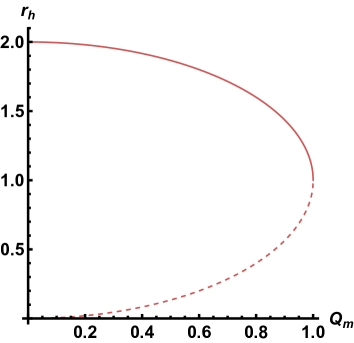
(a) a=0

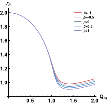
(b) a=2

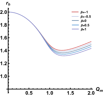
(c) a=10

Figure 1: The relationship between the outer event horizon $r_{+}$(Solid line), inner event horizon $r_{-}$(dashed line) and the charge $Q_{m}$ is shown in the figure. With $M=1$ fixed, $a$ and $\beta$ vary. When $a=0$ the solution reduce to RN black hole.

The Kretschmann scalar reflects the true curvature strength of the gravitational field, which has the following form

$$\mathcal{K}=R^{\mu\nu\rho\sigma}R_{\mu\nu\rho\sigma},$$ (20)

and we can obtain

$$\mathcal{K}=\frac{48}{r^{6}}-\frac{96Q_{m}^{2}}{r^{7}}+\frac{56Q_{m}^{4}}{r^{8}}-\frac{8a(2\pi-\beta)Q_{m}^{4}(19Q_{m}^{2}-14r)}{5\pi r^{12}}+\frac{239a^{2}(\beta-2\pi)^{2}Q_{m}^{8}}{50\pi^{2}r^{16}}.$$ (21)

When $r\to 0$, $\mathcal{K}\to\infty$, it indicates a physical singularity. We observe no divergence of $\mathcal{K}$ at the event horizon, confirming that the event horizon is a coordinate singularity, not a physical one.

IV Electrically charged black holes

We consider the charged solution of our $f(R,T)-EH$ system. The electromagnetic field restricts to an electric charge $Q_{e}$, the symmetry of the spacetime allows the nonvanishing components

$$F_{tr}=-F_{rt}=-\frac{Q_{e}}{r^{2}},$$ (22)

and the invariant reads $F=-Q_{e}^{2}/2r^{4},G=0$. By substitute this to Eq. (9) and Eq. (18) and one can obtain the metric function

$$A_{e}(r)=1-\frac{2M}{r}+\frac{Q_{e}^{2}}{r^{2}}+\frac{r^{2}\beta}{3\pi}+\frac{a\beta Q_{e}^{2}}{\pi r^{2}}+\frac{3Q_{e}^{2}\beta}{2\pi r^{2}}+\frac{aQ_{e}^{4}}{30r^{6}}+\frac{a\beta Q_{e}^{4}}{60\pi r^{6}},$$ (23)

we note that the solution for electric charge significantly differs from that for magnetic charge, with the presence of an $r^{2}$ term. Some studies suggest that this is an effective cosmological constant $\Lambda_{\text{eff}}$ induced by the $f(R,T)$ correction. When $\beta>0$ an anti-de Sitter(adS) spacetime occurs, while $\beta<0$ there exists the cosmological horizon $r_{c}$, and the spacetime is a de Sitter(dS) one.

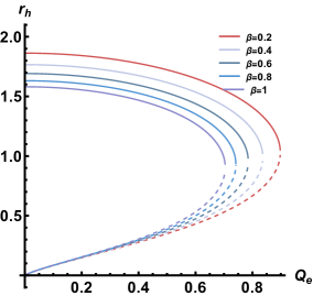
(a) $a=2$

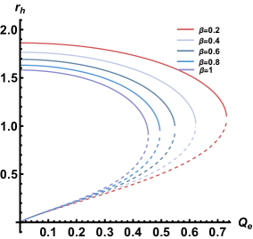
(b) $a=10$

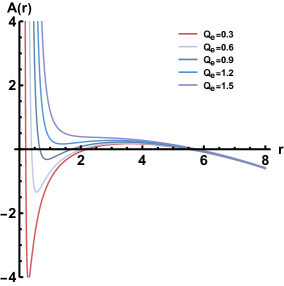
(c) $a=2,\beta=-0.2$

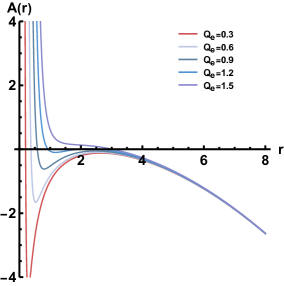
(d) $a=2,\beta=-0.5$

Figure 2: The relationship between the outer event horizon $r_{+}$(Solid line), inner event horizon $r_{-}$(dashed line) and the charge $Q_{e}$ are shown in the figure (a) and (b). For the case where $\beta$ is negative (dS spacetime), the plots of A(r) are shown in (c) and (d). All figures have $M=1$ fixed, $a$ and $\beta$ vary.

The relationship between the charge $Q_{e}$ and the horizon $r_{h}$ for different values of $a$ are illustrates in Fig. 2. For the case where $\beta>0$ (AdS spacetime), as $\beta$ increases, both the inner and outer horizons decrease, and the extremal black hole has smaller $r_{h}$ and $Q_{e}$. An increase in $a$ makes this effect more pronounced. For $\beta<0$ (dS spacetime), a notable feature is the emergence of a cosmological horizon. When $Q_{e}>1$, only the cosmological horizon exists, leading to a naked singularity. As $\beta$ decreases further, an interesting situation arises: for small charges, only the inner horizon exists; for middle charges, there are inner horizons, event horizons, and cosmological horizons; while for large charges, a naked singularity appears with only the cosmological horizon present. This may lead to interesting thermodynamic effects, which will be explored in our future work.

Similarly, we provide the expression for the Kretschmann scalar

$$\begin{split}\mathcal{K}&=\frac{239a^{2}\beta^{2}Q_{e}^{8}}{450\pi^{2}r^{16}}+\frac{478a^{2}\beta Q_{e}^{8}}{225\pi r^{16}}+\frac{478a^{2}Q_{e}^{8}}{225r^{16}}+\frac{304a^{2}\beta Q_{e}^{6}}{15\pi r^{12}}+\frac{152a^{2}\beta^{2}Q_{e}^{6}}{15\pi^{2}r^{12}}+\frac{76a\beta^{2}Q_{e}^{6}}{15\pi^{2}r^{12}}\\ &+\frac{304a\beta Q_{e}^{6}}{15\pi r^{12}}+\frac{304aQ_{e}^{6}}{15r^{12}}-\frac{112a\beta Q_{e}^{4}}{15\pi r^{11}}-\frac{224aQ_{e}^{4}}{15r^{11}}+\frac{508a\beta^{2}Q_{e}^{4}}{9\pi^{2}r^{8}}+\frac{1016a\beta Q_{e}^{4}}{9\pi r^{8}}\\ &+\frac{56a^{2}\beta^{2}Q_{e}^{4}}{\pi^{2}r^{8}}+\frac{14\beta^{2}Q_{e}^{4}}{\pi^{2}r^{8}}+\frac{56\beta Q_{e}^{4}}{\pi r^{8}}+\frac{56Q_{e}^{4}}{r^{8}}-\frac{96a\beta Q_{e}^{2}}{\pi r^{7}}-\frac{48\beta Q_{e}^{2}}{\pi r^{7}}-\frac{96Q_{e}^{2}}{r^{7}}+\frac{48}{r^{6}}+\frac{8\beta^{2}}{3\pi^{2}}.\end{split}$$ (24)

The Kretschmann scalar indicates a coordinate singularity at the horizon, which can be eliminated through a coordinate transformation, while $r=0$ is a physical singularity. Unlike the magnetic charge solution, due to the presence of the “effective cosmological constant” $\Lambda_{\text{eff}}$, the spacetime curvature does not vanish at infinity but approaches a constant value of $8\beta^{2}/(3\pi)$. When $\beta$ is negative, there exists a cosmological horizon $r_{c}$, corresponding to a dS spacetime with positive curvature. When $\beta$ is positive it corresponds to an AdS spacetime.

V Black holes with dyonic EH electrodynamics

In Sections III and IV, we discuss the $f(R,T)$ black hole solutions with magnetic and electric charges within the framework of EH as a low-energy limit of BI theory. For the dyonic case (where both electric and magnetic charges are present), there is some controversy. The approach represented by Yajima et al. [55] starts directly from the Lagrangian of the EH electromagnetic field as a low-energy approximation of BI, obtaining numerical solutions for dyonic black holes and providing a larger parameter space. In contrast, Ruffini et al. [104, 37] start from QED, directly modifying the electric and magnetic charges through vacuum polarization effects, and provide precise screened RN-like analytical solutions. Since this paper focuses on studying the behavior of photons, where QED effects should be considered, we adopt Ruffini’s approach to investigate the dyonic solutions of $f(R,T)$.

In the dyonic case, the gauge potential has the form $A_{\mu}=(A_{t}(r),0,0,Q_{m}\cos\theta)$, where $A_{t}(r)$ represents the contribution of the electric field to the gauge potential, reads [105, 36]

$$A_{t}(r)=-\frac{Q_{e}}{r}\left(1-\frac{2\alpha}{225\pi}\frac{Q_{e}^{2}}{r^{4}E_{c}}-\frac{\alpha}{45\pi}\frac{Q_{m}^{2}}{r^{4}E_{c}}\right),$$ (25)

where $\alpha$ is the fine structure constant and $E_{c}\equiv m_{e}^{2}c^{3}/e\hbar$. For simplicity we set $\eta=2\alpha/225\pi E_{c}$ in our further calculation. Thus, the nonzero components of the Faraday tensor are

$$\begin{split}F_{tr}&=-F_{rt}=-\frac{Q_{e}}{r^{2}}\left(\frac{1}{r^{2}}-\frac{10\eta Q_{e}^{2}+25\eta Q_{m}^{2}}{2r^{2}}\right),\\ F_{\theta\phi}&=-F_{\phi\theta}=Q_{m}\sin\theta,\end{split}$$ (26)

and the invariant of electromagnetic field reads

$$F=\frac{1}{4}F^{\mu\nu}F_{\mu\nu}=\frac{Q_{m}^{2}}{2r^{4}}-\left(\frac{Q_{e}\left(5\eta\left(2Q_{e}^{2}+5Q_{m}^{2}\right)-2r^{4}\right)}{8r^{6}}\right)^{2},$$ (27)

$$G=\frac{1}{4}F_{\mu\nu}*F^{\mu\nu}=-\frac{Q_{m}}{r^{2}}\frac{Q_{e}\left(5\eta\left(2Q_{e}^{2}+5Q_{m}^{2}\right)-2r^{4}\right)}{2r^{6}}.$$ (28)

By substitute this to Eq. (9) and Eq. (18) , we have the analytical solution of the dyonic case

$$\begin{split}&A_{dy}(r)=1-\frac{2M}{r}+\frac{Q_{e}^{2}+Q_{m}^{2}}{r^{2}}-\frac{\eta Q_{e}^{2}\epsilon}{3r^{6}}+\frac{a(Q_{e}^{4}+9Q_{e}^{2}Q_{m}^{2}-3Q_{m}^{4})}{30r^{6}}\\ &-\frac{a\beta(Q_{e}^{2}+7Q_{e}^{2}Q_{m}^{2}-15Q_{m}^{4})}{60\pi r^{6}}+\frac{5\eta\epsilon}{36r^{10}}+\frac{5\pi\eta^{2}Q_{e}^{2}\epsilon^{2}}{36r^{10}}+a\eta Q_{e}^{2}\epsilon\frac{2\beta Q_{e}^{2}-4\pi Q_{e}^{2}+7\beta Q_{m}^{2}-18\pi Q_{m}^{2}}{36\pi r^{10}}\\ &-25a\eta^{2}\epsilon^{2}\frac{6\beta Q_{e}^{2}-12\pi Q_{e}^{2}+7\beta Q_{m}^{2}-18\pi Q_{m}^{2}}{1456\pi r^{14}}-\frac{125a(2\pi-\beta)\eta^{3}Q_{e}^{4}\epsilon^{3}}{1224\pi r^{18}}+\frac{625a(2\pi-\beta)\eta^{4}Q_{e}^{4}\epsilon^{4}}{14784\pi r^{22}},\end{split}$$ (29)

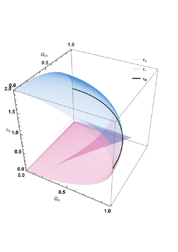
(a) $\beta=-1$

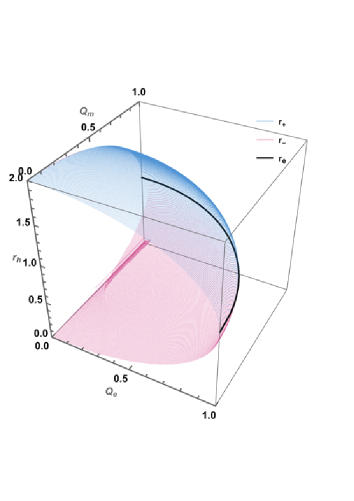
(b) $\beta=1$

Figure 3: The relationship between the outer event horizon $r_{+}$(blue), inner event horizon $r_{-}$(pink), extremal black hole horizon $r_{e}$(black curve) and the charge $Q_{e},Q_{m}$ is shown in the figure. With $M=1$ fixed, $a=0.001768$ and $\beta$ vary.

where $\epsilon=2Q_{e}^{2}+5Q_{m}^{2}$, and the EH parameter $a=0.001768$. We note that when the coupling strength parameters $\eta$ and $a$ vanishes, the spacetime reverts to a Reissner-Nordström (RN)-like solution with magnetic charge [106]. The presence of dyonic charges introduces a coupling term between the magnetic and electric charges, leading to nonlinear interactions between the electric and magnetic fields. Consequently, the spacetime electromagnetic field near the black hole’s horizon exhibits significant deviations from the classical linear Maxwell electromagnetic theory. The coupling of curvature $R$ with matter through the trace of the energy-momentum tensor $T$ further complicates the metric, still resulting in a $1/r^{6}$ and higher order correction. This correction leads to notable observational effects in the strong-field regime, which will be discussed in Section VII.

We present the relationship between $r_{h}$ and the dual charges in Fig. 3. The blue surface represents the outer horizon $r_{+}$, the pink surface represents the inner horizon $r_{-}$, and the black curve at their intersection represents the extremal black hole. Increasing magnetic and electric charges enlarges the inner horizon and shrinks the outer horizon, trending toward an extreme black hole. When $\beta$ is positive, the overall variation trend of the horizon is consistent with that of the $RN$ black hole with electric and magnetic charge. However, when $\beta$ is negative and the $Q_{e},Q_{m}$ are close to each other, a larger $r_{-}$ is obtained.

Similar to the magnetic charge EH field calculation, we provide the Kretschmann curvature scalar $\mathcal{K}$ expression for the dyonic case in the appendix A. Noting that the event horizon $r_{h}$ remains a coordinate singularity, with a physical singularity only at $r\to 0$. Both electric and magnetic charges significantly affect spacetime curvature.

VI energy conditions

In this section we briefly review the energy condition in general relativity and how the energy condition constrains the black hole metric. The energy conditions are expected to impose restrictions on the stress-energy momentum tensor $T_{\mu\nu}$ of matter fields in a physically reasonable model [92]. The origin of energy conditions is the Raychaudhuri equation along with the requirement that gravity is attractive,

$$\frac{d\theta}{d\tau}=-\frac{1}{3}\theta^{2}-\sigma_{\mu\nu}\sigma^{\mu\nu}+\omega_{\mu\nu}\omega^{\mu\nu}-R_{\mu\nu}u^{\mu}u^{\nu},$$ (30)

where $\theta$, $\sigma_{\mu\nu}$ and $\omega_{\mu\nu}$ are the expansion, shear and rotation associated to the vector field $u_{\mu}$ congruent to timelike geodesics. For any timelike 4-vectors $t^{\mu}$, the weak energy condition (WEC) and the strong energy condition (SEC) requires that the energy-momentum tensor satisfies [107]

$$T_{\mu\nu}^{\text{eff}}t^{\mu}t^{\nu}\geq 0\qquad\text{WEC},\\$$ (31)

$$(T_{\mu\nu}^{\text{eff}}-\frac{1}{2}T^{\text{eff}}g_{\mu\nu})t^{\mu}t^{\nu}\geq 0\qquad\text{SEC},\\$$ (32)

the effective stress-energy momentum tensor $T_{\mu\nu}^{\text{eff}}$ and its trace $T^{\text{eff}}$ of magnetic charged and dyonic charged EH $f(R,T)$ spacetime have the form [97]

$$\begin{split}T^{\text{eff}}_{\mu\nu}=&T_{\mu\nu}+\frac{f_{T}}{8\pi}(T_{\mu\nu}+\Theta_{\mu\nu})\\ =&\frac{g_{\mu\nu}}{4\pi}\left(-F+aF^{2}+\frac{7}{4}aG^{2}\right)-\frac{1}{4\pi}\left(-1+2aF\right)F_{\mu\rho}F^{\rho}_{\nu}+\frac{\beta a}{4\pi^{2}}FF_{\mu\nu}F_{\nu}^{\rho},\\ T^{\text{eff}}=&g^{\mu\nu}T_{\mu\nu}^{\text{eff}},\end{split}$$ (33)

where $f_{T}=\partial f(R,T)/\partial T=2\beta$. We choose a static observer with timelike 4-vector $t_{\mu}=(1/\sqrt{A(r)},0,0,0)$ which satisfies $g_{\mu\nu}t^{\mu}t^{\nu}=-1$, and by substituting Eq. (9) and Eq. (33) to Eq. (31) and Eq. (32), we notice that due to $Q_{m}>0$ and $Q_{e}>0$ the spacetime satisfies the WEC outside the event horizon in both magnetic and dyonic charged case.

We note that the spacetime of a magnetic charge black hole violates the SEC and WEC near the singularity, with the boundary of the WEC lying within that of the SEC. The electrically charged AdS black hole ($\beta>0$) globally satisfies both the SEC and WEC, while the electrically charged dS black hole ($\beta<0$) globally satisfies the WEC but only satisfies the SEC in the region near the horizon. For the dyonic black hole, both the SEC and WEC are satisfied outside the inner horizon [92, 108].

VII Geodesics and ISCO of black holes in $f(R,T)$ gravity coupled with EH field

Due to the nonlinear electrodynamics effects, photons propagate along null geodesics in the effective metric $G^{\mu\nu}$ rather than the background metric, which reads [109, 110, 111]

$$G^{\mu\nu}=\mathcal{L}_{FF}F^{\mu}_{\alpha}F^{\alpha\nu}-\mathcal{L}_{F}g^{\mu\nu},$$ (34)

and we can set ansatz of effective metric for spacetime in $f(R,T)$ gravity coupled with EH magnetic monopole and dyonic charge

$$ds^{2}=h(r)(-w(r)dt^{2}+\frac{1}{w(r)}dr^{2}+u(r)(d\theta^{2}+\sin^{2}\theta d\phi^{2})),$$ (35)

and we consider the geodesic equation

$$\frac{d^{2}x^{\mu}}{d\lambda^{2}}+\Gamma^{\mu}_{\rho\sigma}\frac{dx^{\rho}}{d\lambda}\frac{dx^{\sigma}}{d\lambda}=0,$$ (36)

where $\lambda$ is the arbitrary affine parameter, and $\Gamma^{\mu}_{\rho\sigma}$ is the Christoffel symbol. We set $p^{\mu}\equiv dx^{\mu}/d\lambda$ to describe the 4-momentum of the photon. The metric $G_{\mu\nu}$ does not explicitly depend on coordinates $t$ and $\phi$, there exists two conserved quantities, energy $E$ and the angular momentum $L$. The symmetry provides two Killing vector

$$\begin{split}K_{\mu}&=(-h(r)w(r),0,0,0),\\ R_{\mu}&=(0,0,0,h(r)u(r)\sin^{2}\theta),\end{split}$$ (37)

and we could obtain the energy $E$ and the angular momentum $L$ for $\theta=\pi/2$ along the geodesics [112]

$$E=-K_{\mu}p^{\mu}=h(r)w(r)p^{t},\quad L=R_{\mu}p^{\mu}=h(r)u(r)p^{\phi},$$ (38)

substituting Eq. (35) and Eq. (38) to the Lagrangian of photons $\mathcal{L}=\frac{1}{2}g_{\mu\nu}p^{\mu}p^{\nu}=0$, we can derive

$$-\frac{E^{2}}{h(r)w(r)}+\frac{h(r)}{w(r)}(p^{r})^{2}+\frac{L^{2}}{h(r)u(r)}=0.$$ (39)

We define the impact parameter $b\equiv|L|/E$ and setting the affine parameter $\lambda\rightarrow\lambda/L$, one can derive the equation of photon motion

$$\frac{dr}{d\phi}=\pm u(r)\sqrt{\frac{1}{b^{2}}-\frac{w(r)}{u(r)}},$$ (40)

where $\pm$ represents the counterclockwise and clockwise geodesics of the photon.

One can set $V(r)=w(r)/u(r)$ as the effective potential of photons and notice that photons can circle the black hole many times in unstable orbits, called the photon sphere, and it satisfies

$$b_{\text{ph}}=\frac{1}{\sqrt{V(r_{\text{ph}})}},\qquad\frac{dV(r_{\text{ph}})}{dr}=0,\qquad\frac{d^{2}V(r_{\text{ph}})}{dr^{2}}\leq 0,$$ (41)

here $r_{\text{ph}}$ is the radius of photon sphere. Since photon sphere is the innermost unstable circular orbit of photon, one can use the $r_{\text{ph}}$ to describe the radius of the black hole shadow.

As mentioned in Refs. [97, 113], due to the violation of the covariant conservation of the energy-momentum tensor in $f(R,T)$ gravity, i.e.,

$$\nabla^{\mu}T_{\mu\nu}=\frac{f_{T}(R,T)}{8\pi-f_{T}(R,T)}\left[\left(T_{\mu\nu}+\Theta_{\mu\nu}\right)\nabla^{\mu}\ln f_{T}(R,T)+\nabla^{\mu}\Theta_{\mu\nu}-\frac{1}{2}g_{\mu\nu}\nabla^{\mu}T\right]\neq 0,$$ (42)

uncharged massive particles do not follow timelike geodesics, and the equation of motion should be modified by extra force $f^{\alpha}$ as follows, which is considered as the projection of $\nabla^{\mu}T_{\mu\nu}$ in the direction perpendicular to $u^{\mu}$, defined by the projection operator $h_{\mu\alpha}$ [114, 115, 116, 117]

$$\begin{split}&\frac{d^{2}x^{\alpha}}{d\tau^{2}}+\Gamma^{\alpha}_{\mu\nu}\frac{dx^{\mu}}{d\tau}\frac{dx^{\nu}}{d\tau}=f^{\alpha},\\ &f^{\alpha}=\frac{\beta}{4\pi+\beta}\left(h^{\alpha\mu}\nabla_{\mu}\ln\beta+\frac{1}{2}h^{\alpha\mu}\nabla_{\mu}T\right),\end{split}$$ (43)

where the $h_{\mu\alpha}=g_{\mu\alpha}-u_{\mu}u_{\alpha}$ and satisfies $h_{\mu\alpha}u^{\mu}=0$. It is noted that when $\beta=0$, the energy-momentum tensor is covariantly conserved, reverting to Einstein’s gravity, and simultaneously, the extra force $f^{\alpha}=0$, causing the particle’s motion to revert to timelike geodesics. If we simply consider an uncharged test particle (e.g. a dust particle) we can still use the definition of the effective potential in Einstein gravity

$$V_{\text{eff}}\equiv w(r)(1+\frac{L_{m}}{r^{2}}),$$ (44)

where $L_{m}$ is the angular momentum of test particles. The innermost stable circular orbit (ISCO) is the closest distance at which particles around a black hole can maintain a stable circular orbit [118], and satisfies the following conditions

$$\left.\frac{dV_{\text{eff}}(r)}{dr}\right|_{r=r_{\text{ISCO}}}=0,\quad\left.\frac{d^{2}V_{\text{eff}}(r)}{dr^{2}}\right|_{r=r_{\text{ISCO}}}>0.$$ (45)

Inspired by Ref. [119], we could use the orbital plane azimuthal angle $f$ to define the number of orbits $n=f/2\pi$, which depends on the impact parameter b. According to the different values of n, orbits can be categorized into distinct types: direct emission occurs when n ¡ 3/4, lensing ring is formed when 3/4 ¡ n ¡ 5/4, photon ring is established when n ¿ 5/4.

We have provided a general analysis of photon geodesics and the ISCO, and we then will separately study the effective metrics for magnetic, electric, and dyonic solutions, integrate the photon trajectories to plot the geodesic images, and provide numerical solutions for $r_{\text{ISCO}}$.

VII.1 magnetically charged case

by solving the Eq. (34), we have the magnetic charged effective metric

$$w_{m}(r)=A_{m}(r),\quad h_{m}(r)=\frac{\pi r^{4}}{4r^{4}-4aQ_{m}^{2}},\quad u_{m}(r)=\frac{8r^{2}(aQ_{m}^{2}-r^{4})}{8r^{4}-9aQ_{m}^{2}},$$ (46)

$Q_{m}$	0(Sch)	0.1	0.4	0.6	0.8	1
$r_{\text{ph}}$	3	2.99338	2.89054	2.74121	2.49996	2.10741
$r_{\text{ISCO}}$	6	5.98497	5.75284	5.42022	4.89279	4.01471

$\beta$	-1	-0.7	-0.3	0.3	0.7	1
$r_{\text{ph}}$	2.74138	2.74134	2.74130	2.74123	2.74118	2.74114
$r_{\text{ISCO}}$	5.42031	5.42029	5.42027	5.42023	5.42020	5.42018

Table 1: Data of $r_{\text{ph}}$ and $r_{\text{ISCO}}$ of magnetically charged black holes in $f(R,T)$ gravity coupled with EH. Upper table: for different $Q_{m}$ with fixed $M=1,\beta=0.4,a=2$. When $a\rightarrow 0$, the black hole reduce to the RN-like magnetic charged type, when $Q_{m}=0$ the black hole reduce to Schwarzschild. Lower table: for different $\beta$ and fixed $Q_{m}=0.8,a=2$. When $\beta=0$ the black holes reduce to Einstein-Euler-Heisenberg black holes.

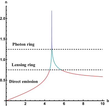
(a) $\beta=-0.6,Q_{m}=0.7$

(b) $\beta=0.6,Q_{m}=0.7$

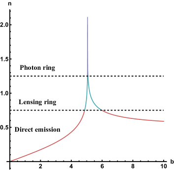
(c) $\beta=0.6,Q_{m}=0.4$

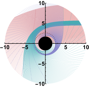
(d) $\beta=-0.6,Q_{m}=0.7$

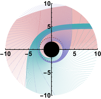
(e) $\beta=0.6,Q_{m}=0.7$

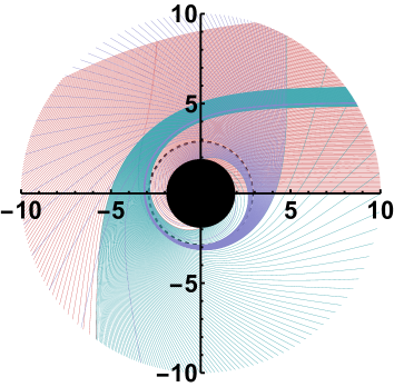
(f) $\beta=0.6,Q_{m}=0.4$

Figure 4: Geodesics structure of magnetically charged black hole in $f(R,T)$ gravity coupled with EH field. Upper line are the number of orbits $n$ with respect to impact parameter $b$. Lower line are the geodesics figure. All fixed $a=2$ and $M=1$.

Since it is not easy to obtain the analytical solution of $r_{\text{ph}},r_{\text{ISCO}}$, here we list the numerical solution in Table. 1. We note that as the $Q_{m}$ increases, $r_{ph}$, and $r_{\text{ISCO}}$ significantly decrease. With fixed electric charge, as $\beta$ increases, the photon sphere radius $r_{ph}$ and $r_{\text{ISCO}}$ both decrease.

The geodesics of photon and the relationship of loop numbers $n$ with respect to impact parameter $b$ are plotted in Fig. 4. Increasing magnetic charge causes photons with lower impact parameter $b$ to achieve a higher $n$, with a significant increase in the proportion of photons in the photon ring and lensing ring, making the overall gravitational lensing effect more pronounced. Increasing the coupling constant $\beta$ enlarges the horizon radius, shrinks the photon sphere, and increases spacetime curvature near the photon sphere, resulting in photons in the photon ring having a higher number of orbits $n$.

VII.2 electrically charged case

One can still provide the effective metric reads

$$w_{e}(r)=A_{e}(r),\quad h_{e}(r)=\frac{2\pi r^{4}}{9aQ_{e}^{2}+8r^{4}},\quad u_{e}(r)=\frac{r^{2}(9aQ_{e}^{2}+8r^{4})}{8aQ_{e}^{2}+8r^{4}},$$ (47)

based on the effective metric and the previously mentioned definitions of the photon sphere radius(or shadow radius) $r_{\text{ph}}$ and ISCO, we provide the reference values in Table 2.

$Q_{e}$	0	0.2	0.4	0.6	0.8	0.9
$r_{\text{ph}}$	3	2.96076	2.83616	2.59747	2.21254	-
$r_{\text{ISCO}}$	3.89065	3.84351	3.69403	3.40893	2.85593	2.11178

$\beta$	-1	-0.7	-0.3	0.3	0.7	1
$r_{\text{ph}}$	2.73071	2.32297	2.80497	2.67075	2.57193	2.49135
$r_{\text{ISCO}}$	3.57214	3.43032	4.05537	3.60397	3.36013	3.22798

Table 2: Data of $r_{\text{ph}}$ and $r_{\text{ISCO}}$ of black holes in $f(R,T)$ gravity coupled with EH electrical charge. Upper table: for different $Q_{e}$ with fixed $M=1,a=2,\beta=0.6$. Lower table: for different $\beta$ and fixed $M=1,a=2,Q_{e}=0.6$. When $\beta\rightarrow 0$, the black hole reduce to the EH electrical charged black hole.

We can conclude that for $\beta>0$(AdS spacetime), as $Q_{e}$ and $\beta$ increases, both the $r_{\text{ph}}$ decrease significantly. For $\beta<0$(dS spacetime), when there exists singularity (e.g. $\beta=1,0.7$), the photon sphere is outside the cosmological horizon $r_{c}$ and it means there is no photon sphere in this spacetime; when there remains $r_{-}$, $r_{+}$ and $r_{c}$, the $r_{\text{ph}}$ is larger than that of the singularity.

We present the orbit number $n$ and geodesics of a dS solution in Fig. 5(a), 5(b) and 5(e), 5(f). Due to the existence of the cosmological horizon, we only consider photons with $r<r_{c}$, as photons beyond this are not causally connected to our universe. We note that an increase in $|\beta|$ significantly reduces the cosmological horizon while markedly increasing the impact parameters of the photon ring and the lensing ring. Within the range of impact parameters ($0<b<10$), most directly emission photons will fall into the black hole.

VII.3 dyonic charged case

From the Eq. (34) we can obtain the effective metric of dyonic charged black hole, which reads

$$\begin{split}w_{\text{dy}}(r)&=A_{\text{dy}}(r),\\ h_{\text{dy}}(r)&=\frac{8\pi r^{12}}{225a\eta^{2}Q_{e}^{2}\epsilon^{2}-180a\eta Q_{e}^{2}r^{4}\epsilon+4r^{8}\left(9aQ_{e}^{2}-8aQ_{m}^{2}+8r^{4}\right)},\\ u_{\text{dy}}(r)&=\frac{r^{10}\left(17aQ_{m}^{2}-8r^{4}\right)}{8a\left(50\eta^{2}Q_{e}^{2}\epsilon^{2}+r^{8}\left(8Q_{e}^{2}-9Q_{m}^{2}\right)-40\eta Q_{e}^{2}r^{4}\epsilon\right)+64r^{12}}+\frac{9r^{2}}{8}.\end{split}$$ (48)

For the dyonic EH electromagnetic field in Table. 3, similar to the magnetic charge, increasing electric and magnetic charges significantly reduces $r_{h}$, $r_{ph}$, and $r_{\text{ISCO}}$. As $\beta$ increases, $r_{h}$ first decreases then increases, while the photon sphere and ISCO approach the event horizon.

$Q_{e}$	0	0.2	0.4	0.6	0.8	0.9
$r_{\text{ph}}$	2.82288	2.79229	2.69583	2.51489	2.18557	1.86055
$r_{\text{ISCO}}$	5.60664	5.53983	5.33155	4.95207	4.31323	3.80142

Table 3: Data of $r_{\text{h}}$, $r_{\text{ph}}$, $b_{\text{ph}}$ of black holes in $f(R,T)$ gravity coupled with EH dyonic electromagnetic field, for different $Q_{e}$ with fixed $M=1,Q_{m}=0.7,\beta=0.6,\eta=2\alpha/225\pi,a=0.001786$.

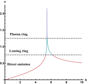
(a) $\beta=-0.1,Q_{e}=0.7$

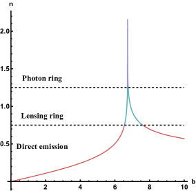
(b) $\beta=-0.2,Q_{e}=0.7$

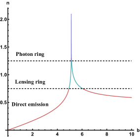
(c) $Q_{e}=0.2,Q_{m}=0.2$

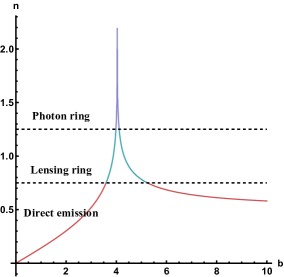
(d) $Q_{e}=0.7,Q_{m}=0.7$

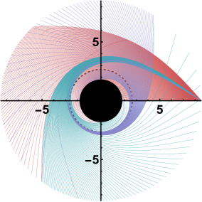
(e) $\beta=-0.1,Q_{e}=0.7$

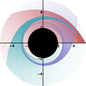
(f) $\beta=-0.2,Q_{e}=0.7$

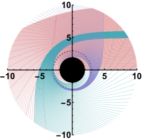
(g) $Q_{e}=0.2,Q_{m}=0.2$

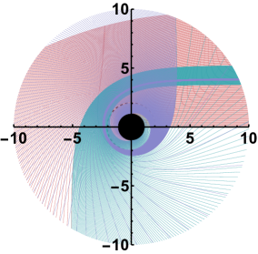
(h) $Q_{m}=0.7,Q_{m}=0.7$

Figure 5: Geodesics structure of electrically and dyonic charged black hole in $f(R,T)$ gravity coupled with EH field. Upper line are the number of orbits $n$ with respect to impact parameter $b$. Lower line are the geodesics figure. All fixed $a=2$ and $M=1$, and we fixed $\beta=0.6$ for dyonic case in the right columns.

The geodesics figure are shown in the right two columns of Fig. 5, increasing magnetic and electric charges causes photons with lower impact parameter $b$ to achieve a higher number of orbital loops $n$, with a significant increase in the proportion of photons in the photon ring and lensing ring. The Increasing coupling constant $\beta$ significantly enhances the proportion of the photon ring and lensing ring, and photon trajectories with smaller impact parameters exhibit highly pronounced light deflection. This indicates that the introduction of electric charge amplifies the matter field’s influence on the gravitational field, particularly evident at higher coupling strengths.

VIII Conclusion and discussion

In this study, we consider the $f(R,T)$-Euler-Heisenberg action within the framework of $f(R,T)$ gravity and obtain the field equations. We present the energy-momentum tensor $T_{\mu\nu}$ and $\Theta_{\mu\nu}$, simplifying the field equations using a linearly coupled $f(R,T)$ form. Two physical interpretations of the Euler-Heisenberg (EH) theory are discussed: as a low-energy limit of Born-Infeld (BI) theory and as a vacuum polarization QED correction. Under the first interpretation, we derive analytical solutions for magnetically and electrically charged black holes; under the second, we propose an analytical solution for a dyonic black hole. The magnetic and dyonic solutions are asymptotically flat astrophysical black hole solutions, while the electric charge solution includes an effective cosmological constant term, with the coupling parameter $\beta$ determining its AdS/dS nature. We analyze the properties of the horizons and singularities of these black holes and briefly explore the energy conditions.

Subsequently, we derive effective metrics influenced by nonlinear electromagnetic fields and investigate photon trajectories and massive particle dynamics for the three black hole solutions. In the magnetic charge solution, increases in the magnetic charge $Q_{m}$ and coupling strength $\beta$ reduce the shadow radius (photon sphere radius, $r_{\text{ph}}$). In photon dynamics, photons with smaller impact parameters $b$ exhibit a higher number of orbits, with a larger proportion contributing to the photon and lensing rings, resulting in increased large-angle deflection in geodesic images.

In the electrically charged de Sitter (dS) solution, the electric charge $Q_{e}$ and $\beta$ significantly affect the spacetime metric, leading to three scenarios: (i) a naked singularity; (ii) a dS black hole with an inner horizon $r_{-}$, outer horizon $r_{+}$, and cosmological horizon $r_{c}$; (iii) an extreme dS black hole with a cosmological horizon $r_{c}$. For the naked singularity, the photon sphere lies beyond the cosmological horizon, implying no stable photon circular orbits exist in this spacetime. In the dS black hole case, increases in $Q_{e}$ and $|\beta|$ reduce the shadow radius. We observe that a larger $|\beta|$ substantially shrinks the cosmological horizon and significantly increases the impact parameters for both the photon ring and the lensing ring. Within the impact parameter range of $0<b<10$, the majority of directly emitted photons are captured by the black hole.

In the dyonic model, increases in both electric and magnetic charges similarly reduce the shadow radius, with photons at smaller $b$ exhibiting more orbits and enhanced contributions to the photon and lensing rings. For large dyonic charges, an increase in $\beta$ significantly enhances the proportion of photons in the photon and lensing rings.

Black holes coupled with EH nonlinear electrodynamics in the $f(R,T)$ gravity differ from those in the EEH framework in our toy model. The AdS/dS solutions are highly sensitive to parameter choices, potentially exhibiting intriguing thermodynamic effects and providing insights for conformal field theory (CFT). The dyonic black hole, derived from QED corrections, exhibits direct observational signatures. In future work, we will compare these results with observational data [84] and contrast them with EEH dyonic black holes, potentially offering references for $f(R,T)$ research and next-generation Event Horizon Telescope observation.

Appendix A Kretschmann scalar of dyonic EH black hole in $f(R,T)$ gravity

Here we give the Kretschmann scalar of dyonic EH black hole in $f(R,T)$ gravity, reads

$$\begin{split}&\mathcal{K}_{dyonic}=\frac{1399609375a^{2}\left(2Q_{e}^{2}+5Q_{m}^{2}\right)^{8}(\beta-2\pi)^{2}\eta^{8}Q_{e}^{8}}{3035648\pi^{2}r^{48}}+\frac{239a^{2}\beta^{2}Q_{e}^{8}}{450\pi^{2}r^{16}}+\frac{478a^{2}Q_{e}^{8}}{225r^{16}}-\frac{478a^{2}\beta Q_{e}^{8}}{225\pi r^{16}}\\ &-\frac{852734375a^{2}\left(2Q_{e}^{2}+5Q_{m}^{2}\right)^{7}(\beta-2\pi)^{2}\eta^{7}Q_{e}^{8}}{565488\pi^{2}r^{44}}+15625a^{2}\left(2Q_{e}^{2}+5Q_{m}^{2}\right)^{6}(2\pi-\beta)\times\\ &\frac{\left(-1457769314\beta Q_{e}^{2}+2915538628\pi Q_{e}^{2}+1887280398\pi Q_{m}^{2}-733942377Q_{m}^{2}\beta\right)\eta^{6}Q_{e}^{6}}{10497719232\pi^{2}r^{40}}\\ &+\frac{1673a^{2}Q_{m}^{2}\beta^{2}Q_{e}^{6}}{225\pi^{2}r^{16}}+\frac{956a^{2}Q_{m}^{2}Q_{e}^{6}}{25r^{16}}-\frac{7648a^{2}Q_{m}^{2}\beta Q_{e}^{6}}{225\pi r^{16}}\\ &-\frac{625a^{2}\left(2Q_{e}^{2}+5Q_{m}^{2}\right)^{5}(2\pi-\beta)\left(-1762498\beta Q_{e}^{2}+3524996\pi Q_{e}^{2}+6849522\pi Q_{m}^{2}-2663703Q_{m}^{2}\beta\right)\eta^{5}Q_{e}^{6}}{612612\pi^{2}r^{36}}\\ &+\frac{4541a^{2}Q_{m}^{4}\beta^{2}Q_{e}^{4}}{450\pi^{2}r^{16}}+\frac{478a^{2}Q_{m}^{4}Q_{e}^{4}}{3r^{16}}-\frac{478a^{2}Q_{m}^{4}\beta Q_{e}^{4}}{5\pi r^{16}}-\frac{25a^{2}\left(2Q_{e}^{2}+5Q_{m}^{2}\right)^{3}\eta^{3}Q_{e}^{4}}{83538\pi^{2}r^{28}}\times\\ &(\left(1073498Q_{e}^{4}+5402474Q_{m}^{2}Q_{e}^{2}+1170771Q_{m}^{4}\right)\beta^{2}-4\pi\left(1073498Q_{e}^{4}+6174256Q_{m}^{2}Q_{e}^{2}+3236877Q_{m}^{4}\right)\beta\\ &+4\pi^{2}\left(1073498Q_{e}^{4}+6946038Q_{m}^{2}Q_{e}^{2}+5604699Q_{m}^{4}\right))+\frac{24856a^{2}Q_{m}^{6}\beta Q_{e}^{2}}{75\pi r^{16}}-\frac{2868a^{2}Q_{m}^{6}Q_{e}^{2}}{25r^{16}}\\ &-\frac{1673a^{2}Q_{m}^{6}\beta^{2}Q_{e}^{2}}{15\pi^{2}r^{16}}-608a^{2}\left(2Q_{e}^{2}+5Q_{m}^{2}\right)\left(-2\beta Q_{e}^{2}+4\pi Q_{e}^{2}+18\pi Q_{m}^{2}-7Q_{m}^{2}\beta\right)\times\\ &\frac{\left(2\pi\left(Q_{e}^{4}+9Q_{m}^{2}Q_{e}^{2}-3Q_{m}^{4}\right)-\left(Q_{e}^{4}+7Q_{m}^{2}Q_{e}^{2}-15Q_{m}^{4}\right)\beta\right)\eta Q_{e}^{2}}{135\pi^{2}r^{20}}+\frac{239a^{2}Q_{m}^{8}\beta^{2}}{2\pi^{2}r^{16}}+\frac{a^{2}Q_{e}^{2}\left(2Q_{e}^{2}+5Q_{m}^{2}\right)^{2}\eta^{2}}{9828\pi^{2}r^{24}}\times\\ &(\left(688438Q_{e}^{6}+5179741Q_{m}^{2}Q_{e}^{4}+2533753Q_{m}^{4}Q_{e}^{2}-5410125Q_{m}^{6}\right)\beta^{2}-4\pi(688438Q_{e}^{6}+5919704Q_{m}^{2}Q_{e}^{4}\\ &+6437511Q_{m}^{4}Q_{e}^{2}-4018950Q_{m}^{6})\beta+4\pi^{2}\left(688438Q_{e}^{6}+6659667Q_{m}^{2}Q_{e}^{4}+10926657Q_{m}^{4}Q_{e}^{2}-1391175Q_{m}^{6}\right))\\ &+\frac{125a^{2}Q_{e}^{4}\left(2Q_{e}^{2}+5Q_{m}^{2}\right)^{4}}{4013833824\pi^{2}r^{32}}(\left(30255060830Q_{e}^{4}+91494873274Q_{m}^{2}Q_{e}^{2}+6036696855Q_{m}^{4}\right)\beta^{2}\\ &-4\pi\left(30255060830Q_{e}^{4}+104565569456Q_{m}^{2}Q_{e}^{2}+17900307369Q_{m}^{4}\right)\beta\\ &+4\pi^{2}\left(30255060830Q_{e}^{4}+117636265638Q_{m}^{2}Q_{e}^{2}+31463714223Q_{m}^{4}\right))\eta^{4}+\frac{432}{54r^{24}}\times\\ &((7\left(Q_{e}^{2}+Q_{m}^{2}\right)^{2}-12r\left(Q_{e}^{2}+Q_{m}^{2}\right)+6r^{2})r^{16}-576Q_{e}^{2}\left(2Q_{e}^{2}+5Q_{m}^{2}\right)\left(19\left(Q_{e}^{2}+Q_{m}^{2}\right)-14r\right)\eta r^{12}\\ &+24Q_{e}^{2}\left(2Q_{e}^{2}+5Q_{m}^{2}\right)^{2}\left(943Q_{e}^{2}+465Q_{m}^{2}-330r\right)\eta^{2}r^{8}-24320Q_{e}^{4}\left(2Q_{e}^{2}+5Q_{m}^{2}\right)^{3}\eta^{3}r^{4}\\ &+13025Q_{e}^{4}\left(2Q_{e}^{2}+5Q_{m}^{2}\right)^{4}\eta^{4})+\frac{478a^{2}Q_{m}^{8}}{25r^{16}}-\frac{478a^{2}Q_{m}^{8}\beta}{5\pi r^{16}}+\frac{a}{27567540\pi r^{36}}\times\\ &((14702688\left(19\left(Q_{e}^{2}+Q_{m}^{2}\right)-14r\right)\left(2\pi\left(Q_{e}^{4}+9Q_{m}^{2}Q_{e}^{2}-3Q_{m}^{4}\right)-\left(Q_{e}^{4}+7Q_{m}^{2}Q_{e}^{2}-15Q_{m}^{4}\right)\beta\right)r^{24}\\ &-2450448Q_{e}^{2}\left(2Q_{e}^{2}+5Q_{m}^{2}\right)(2\pi\left(1169Q_{e}^{4}+7266Q_{m}^{2}Q_{e}^{2}+3468Q_{m}^{4}-330\left(2Q_{e}^{2}+9Q_{m}^{2}\right)r\right)\\ &+\left(-1169Q_{e}^{4}+\left(660r-5858Q_{m}^{2}\right)Q_{e}^{2}+330\left(Q_{m}^{4}+7rQ_{m}^{2}\right)\right)\beta)\eta r^{20}\\ &+44880Q_{e}^{2}\left(2Q_{e}^{2}+5Q_{m}^{2}\right)^{2}(6\pi\left(99546Q_{e}^{4}+352605Q_{m}^{2}Q_{e}^{2}+73243Q_{m}^{4}-20250\left(2Q_{e}^{2}+3Q_{m}^{2}\right)r\right)\\ &+\left(-298638Q_{e}^{4}-861445Q_{m}^{2}Q_{e}^{2}+4305Q_{m}^{4}+20250\left(6Q_{e}^{2}+7Q_{m}^{2}\right)r\right)\beta)\eta^{2}r^{16}\\ &-6600Q_{e}^{4}\left(2Q_{e}^{2}+5Q_{m}^{2}\right)^{3}(2\pi\left(5310637Q_{e}^{2}+9445479Q_{m}^{2}-1296750r\right)+\\ &\left(-5310637Q_{e}^{2}-7763567Q_{m}^{2}+1296750r\right)\beta)\eta^{3}r^{12}+3750Q_{e}^{4}\left(2Q_{e}^{2}+5Q_{m}^{2}\right)^{4}\times\\ &(-14384659\beta Q_{e}^{2}+28769318\pi Q_{e}^{2}+1836\pi\left(10312Q_{m}^{2}-1495r\right)+306\left(4485r-25513Q_{m}^{2}\right)\beta)\eta^{4}r^{8}\\ &-46911353125Q_{e}^{6}\left(2Q_{e}^{2}+5Q_{m}^{2}\right)^{5}(2\pi-\beta)\eta^{5}r^{4}+18305015625Q_{e}^{6}\left(2Q_{e}^{2}+5Q_{m}^{2}\right)^{6}(2\pi-\beta)\eta^{6})).\end{split}$$ (49)

References

- [1] B. P. Abbott et al. Observation of Gravitational Waves from a Binary Black Hole Merger. Phys. Rev. Lett., 116(6):061102, 2016.
- [2] B. P. Abbott et al. Multi-messenger Observations of a Binary Neutron Star Merger. Astrophys. J. Lett., 848(2):L12, 2017.
- [3] Maximo Banados, Claudio Teitelboim, and Jorge Zanelli. The Black hole in three-dimensional space-time. Phys. Rev. Lett., 69:1849–1851, 1992.
- [4] F. Lucchin and S. Matarrese. Power Law Inflation. Phys. Rev. D, 32:1316, 1985.
- [5] Edmund J. Copeland, M. Sami, and Shinji Tsujikawa. Dynamics of dark energy. Int. J. Mod. Phys. D, 15:1753–1936, 2006.
- [6] David J. E. Marsh. Axion Cosmology. Phys. Rept., 643:1–79, 2016.
- [7] David H. Weinberg, Michael J. Mortonson, Daniel J. Eisenstein, Christopher Hirata, Adam G. Riess, and Eduardo Rozo. Observational Probes of Cosmic Acceleration. Phys. Rept., 530:87–255, 2013.
- [8] N. Aghanim et al. Planck 2018 results. VI. Cosmological parameters. Astron. Astrophys., 641:A6, 2020. [Erratum: Astron.Astrophys. 652, C4 (2021)].
- [9] D. N. Spergel et al. First year Wilkinson Microwave Anisotropy Probe (WMAP) observations: Determination of cosmological parameters. Astrophys. J. Suppl., 148:175–194, 2003.
- [10] K. A. Olive et al. Review of Particle Physics. Chin. Phys. C, 38:090001, 2014.
- [11] Douglas Clowe, Marusa Bradac, Anthony H. Gonzalez, Maxim Markevitch, Scott W. Randall, Christine Jones, and Dennis Zaritsky. A direct empirical proof of the existence of dark matter. Astrophys. J. Lett., 648:L109–L113, 2006.
- [12] Antonio De Felice and Shinji Tsujikawa. f(R) theories. Living Rev. Rel., 13:3, 2010.
- [13] S. Nojiri, S. D. Odintsov, and V. K. Oikonomou. Modified Gravity Theories on a Nutshell: Inflation, Bounce and Late-time Evolution. Phys. Rept., 692:1–104, 2017.
- [14] Shin’ichi Nojiri and Sergei D. Odintsov. Unified cosmic history in modified gravity: from F(R) theory to Lorentz non-invariant models. Phys. Rept., 505:59–144, 2011.
- [15] Vincent R. Siggia and Eric D. Carlson. Comparison of f(R,T) gravity with type Ia supernovae data. Phys. Rev. D, 111(2):024074, 2025.
- [16] S. Perlmutter et al. Discovery of a supernova explosion at half the age of the Universe and its cosmological implications. Nature, 391:51–54, 1998.
- [17] S. Perlmutter et al. Measurements of and from 42 High Redshift Supernovae. Astrophys. J., 517:565–586, 1999.
- [18] Prabir Rudra and Kinsuk Giri. Observational constraint in gravity from the cosmic chronometers and some standard distance measurement parameters. Nucl. Phys. B, 967:115428, 2021.
- [19] M. Sharif, S. Rani, and R. Myrzakulov. Analysis of gravity models through energy conditions. Eur. Phys. J. Plus, 128:123, 2013.
- [20] G. A. Carvalho, R. V. Lobato, P. H. R. S. Moraes, José D. V. Arbañil, R. M. Marinho, E. Otoniel, and M. Malheiro. Stellar equilibrium configurations of white dwarfs in the f(R, T) gravity. Eur. Phys. J. C, 77(12):871, 2017.
- [21] Snehasish Bhattacharjee. White dwarf cooling in f(R,T) gravity. Int. J. Mod. Phys. A, 39(05n06):2450026, 2024.
- [22] Debabrata Deb, Sergei V. Ketov, Maxim Khlopov, and Saibal Ray. Study on charged strange stars in gravity. JCAP, 10:070, 2019.
- [23] Juan M. Z. Pretel, Sergio E. Jorás, Ribamar R. R. Reis, and José D. V. Arbañil. Radial oscillations and stability of compact stars in gravity. JCAP, 04:064, 2021.
- [24] L. Sebastiani, S. Vagnozzi, and R. Myrzakulov. Mimetic gravity: a review of recent developments and applications to cosmology and astrophysics. Adv. High Energy Phys., 2017:3156915, 2017.
- [25] Min-Xing Xu, Tiberiu Harko, and Shi-Dong Liang. Quantum Cosmology of gravity. Eur. Phys. J. C, 76(8):449, 2016.
- [26] Ratbay Myrzakulov. FRW Cosmology in F(R,T) gravity. Eur. Phys. J. C, 72:2203, 2012.
- [27] Guo-He Li, Yeqi Fang, Yuchi Wu, and Jun Tao. Wormhole Solutions and pre-inflationary in Gravity with Axion Fields. 6 2025.
- [28] Amin Salehi and S. Aftabi. Searching for a Cosmological Preferred Axis in complicated class of cosmological models:Case study model. JHEP, 09:140, 2016.
- [29] Mubasher Jamil, D. Momeni, Muhammad Raza, and Ratbay Myrzakulov. Reconstruction of some cosmological models in f(R,T) gravity. Eur. Phys. J. C, 72:1999, 2012.
- [30] Hamid Shabani and Mehrdad Farhoudi. Cosmological and Solar System Consequences of f(R,T) Gravity Models. Phys. Rev. D, 90(4):044031, 2014.
- [31] M. E. S. Alves, P. H. R. S. Moraes, J. C. N. de Araujo, and M. Malheiro. Gravitational waves in and theories of gravity. Phys. Rev. D, 94(2):024032, 2016.
- [32] Ismail Soudi, Gabriel Farrugia, Viktor Gakis, Jackson Levi Said, and Emmanuel N. Saridakis. Polarization of gravitational waves in symmetric teleparallel theories of gravity and their modifications. Phys. Rev. D, 100(4):044008, 2019.
- [33] C. P. Singh and Pankaj Kumar. Friedmann model with viscous cosmology in modified gravity theory. Eur. Phys. J. C, 74:3070, 2014.
- [34] W. Heisenberg and H. Euler. Consequences of Dirac’s theory of positrons. Z. Phys., 98(11-12):714–732, 1936.
- [35] Julian S. Schwinger. On gauge invariance and vacuum polarization. Phys. Rev., 82:664–679, 1951.
- [36] Daniela Magos, Nora Bretón, and Alfredo Macías. Orbits in static magnetically and dyonically charged Einstein-Euler-Heisenberg black hole spacetimes. Phys. Rev. D, 108(6):064014, 2023.
- [37] Remo Ruffini, Yuan-Bin Wu, and She-Sheng Xue. Einstein-Euler-Heisenberg Theory and charged black holes. Phys. Rev. D, 88:085004, 2013.
- [38] Y. Meng, B. B. Chen, and J. Tang. Cooling–heating phase transition of the Euler–Heisenberg-AdS black hole. Mod. Phys. Lett. A, 36(23):2150165, 2021.
- [39] Daniel Amaro and Alfredo Macías. Geodesic structure of the Euler-Heisenberg static black hole. Phys. Rev. D, 102(10):104054, 2020.
- [40] Daniel Amaro, Nora Breton, Claus Lämmerzahl, and Alfredo Macías. Thermodynamics of the Einstein-Euler-Heisenberg rotating black hole. Phys. Rev. D, 105(10):104046, 2022.
- [41] Daniel Amaro and Alfredo Macías. Exact lens equation for the Einstein-Euler-Heisenberg static black hole. Phys. Rev. D, 106(6):064010, 2022.
- [42] Nora Breton, Claus Lämmerzahl, and Alfredo Macías. Type-D solutions of the Einstein-Euler-Heisenberg nonlinear electrodynamics with a cosmological constant. Phys. Rev. D, 107(6):064026, 2023.
- [43] Daniel Amaro, Claus Lämmerzahl, and Alfredo Macías. Particle motion in the Einstein-Euler-Heisenberg rotating black hole spacetime. Phys. Rev. D, 107(8):084040, 2023.
- [44] Fredrick W. Cotton. A generalization of the Einstein–Maxwell equations. Eur. Phys. J. Plus, 136(2):162, 2021.
- [45] Gert Brodin, Mattias Marklund, and Lennart Stenflo. Proposal for Detection of QED Vacuum Nonlinearities in Maxwell’s Equations by the Use of Waveguides. Phys. Rev. Lett., 87:171801, 2001.
- [46] G. Boillat. Nonlinear electrodynamics - Lagrangians and equations of motion. J. Math. Phys., 11(3):941–951, 1970.
- [47] P. Stehle and P. G. DeBaryshe. Quantum Electrodynamics and the Correspondence Principle. Phys. Rev., 152(4):1135, 1966.
- [48] G. W. Gibbons and D. A. Rasheed. Electric - magnetic duality rotations in nonlinear electrodynamics. Nucl. Phys. B, 454:185–206, 1995.
- [49] E. S. Fradkin and Arkady A. Tseytlin. Nonlinear Electrodynamics from Quantized Strings. Phys. Lett. B, 163:123–130, 1985.
- [50] Ahmed Abouelsaood, Curtis G. Callan, Jr., C. R. Nappi, and S. A. Yost. Open strings in background gauge fields. Nucl. Phys. B, 280:599–624, 1987.
- [51] Arkady A. Tseytlin. On nonAbelian generalization of Born-Infeld action in string theory. Nucl. Phys. B, 501:41–52, 1997.
- [52] A. García D., H. Salazar I., and J. F. Plebański. Type-D solutions of the Einstein and Born-Infeld nonlinear-electrodynamics equations. Nuovo Cim. B, 84(1):65–90, 1984.
- [53] M. Demianski. STATIC ELECTROMAGNETIC GEON. Found. Phys., 16:187–190, 1986.
- [54] Z. Bern and A. G. Morgan. Supersymmetry relations between contributions to one loop gauge boson amplitudes. Phys. Rev. D, 49:6155–6163, 1994.
- [55] Hiroki Yajima and Takashi Tamaki. Black hole solutions in Euler-Heisenberg theory. Phys. Rev. D, 63:064007, 2001.
- [56] Alireza Allahyari, Mohsen Khodadi, Sunny Vagnozzi, and David F. Mota. Magnetically charged black holes from non-linear electrodynamics and the Event Horizon Telescope. JCAP, 02:003, 2020.
- [57] Sunny Vagnozzi et al. Horizon-scale tests of gravity theories and fundamental physics from the Event Horizon Telescope image of Sagittarius A. Class. Quant. Grav., 40(16):165007, 2023.
- [58] Guan-Ru Li, Sen Guo, and En-Wei Liang. High-order QED correction impacts on phase transition of the Euler-Heisenberg AdS black hole. Phys. Rev. D, 106(6):064011, 2022.
- [59] Daniela Magos and Nora Bretón. Thermodynamics of the Euler-Heisenberg-AdS black hole. Phys. Rev. D, 102(8):084011, 2020.
- [60] Jose Luis Blázquez-Salcedo, Daniela D. Doneva, Sarah Kahlen, Jutta Kunz, Petya Nedkova, and Stoytcho S. Yazadjiev. Polar quasinormal modes of the scalarized Einstein-Gauss-Bonnet black holes. Phys. Rev. D, 102(2):024086, 2020.
- [61] Thanasis Karakasis, George Koutsoumbas, Andri Machattou, and Eleftherios Papantonopoulos. Magnetically charged Euler-Heisenberg black holes with scalar hair. Phys. Rev. D, 106(10):104006, 2022.
- [62] Marco Maceda and Alfredo Macías. Non-commutative inspired black holes in Euler–Heisenberg non-linear electrodynamics. Phys. Lett. B, 788:446–452, 2019.
- [63] Gustavo Gutierrez-Cano and Gustavo Niz. Euler-heisenberg black holes in einsteinian cubic gravity. Gen. Rel. Grav., 57(1):8, 2025.
- [64] H. Rehman, G. Abbas, Tao Zhu, and G. Mustafa. Matter accretion onto the magnetically charged Euler–Heisenberg black hole with scalar hair. Eur. Phys. J. C, 83(9):856, 2023.
- [65] Nora Bretón and L. A. López. Birefringence and quasinormal modes of the Einstein-Euler-Heisenberg black hole. Phys. Rev. D, 104(2):024064, 2021.
- [66] Kazunori Akiyama et al. First Sagittarius A* Event Horizon Telescope Results. I. The Shadow of the Supermassive Black Hole in the Center of the Milky Way. Astrophys. J. Lett., 930(2):L12, 2022.
- [67] Kazunori Akiyama et al. First Sagittarius A* Event Horizon Telescope Results. II. EHT and Multiwavelength Observations, Data Processing, and Calibration. Astrophys. J. Lett., 930(2):L13, 2022.
- [68] Kazunori Akiyama et al. First Sagittarius A* Event Horizon Telescope Results. III. Imaging of the Galactic Center Supermassive Black Hole. Astrophys. J. Lett., 930(2):L14, 2022.
- [69] Kazunori Akiyama et al. First Sagittarius A* Event Horizon Telescope Results. IV. Variability, Morphology, and Black Hole Mass. Astrophys. J. Lett., 930(2):L15, 2022.
- [70] Kazunori Akiyama et al. First Sagittarius A* Event Horizon Telescope Results. V. Testing Astrophysical Models of the Galactic Center Black Hole. Astrophys. J. Lett., 930(2):L16, 2022.
- [71] Kazunori Akiyama et al. First Sagittarius A* Event Horizon Telescope Results. VI. Testing the Black Hole Metric. Astrophys. J. Lett., 930(2):L17, 2022.
- [72] Kazunori Akiyama et al. First M87 Event Horizon Telescope Results. I. The Shadow of the Supermassive Black Hole. Astrophys. J. Lett., 875:L1, 2019.
- [73] Kazunori Akiyama et al. First M87 Event Horizon Telescope Results. II. Array and Instrumentation. Astrophys. J. Lett., 875(1):L2, 2019.
- [74] Kazunori Akiyama et al. First M87 Event Horizon Telescope Results. III. Data Processing and Calibration. Astrophys. J. Lett., 875(1):L3, 2019.
- [75] Kazunori Akiyama et al. First M87 Event Horizon Telescope Results. IV. Imaging the Central Supermassive Black Hole. Astrophys. J. Lett., 875(1):L4, 2019.
- [76] Kazunori Akiyama et al. First M87 Event Horizon Telescope Results. V. Physical Origin of the Asymmetric Ring. Astrophys. J. Lett., 875(1):L5, 2019.
- [77] Kazunori Akiyama et al. First M87 Event Horizon Telescope Results. VI. The Shadow and Mass of the Central Black Hole. Astrophys. J. Lett., 875(1):L6, 2019.
- [78] Andrey A. Shoom. Metamorphoses of a photon sphere. Phys. Rev. D, 96(8):084056, 2017.
- [79] J. L. Synge. The Escape of Photons from Gravitationally Intense Stars. Mon. Not. Roy. Astron. Soc., 131(3):463–466, 1966.
- [80] James M. Bardeen, William H. Press, and Saul A Teukolsky. Rotating black holes: Locally nonrotating frames, energy extraction, and scalar synchrotron radiation. Astrophys. J., 178:347, 1972.
- [81] J. P. Luminet. Image of a spherical black hole with thin accretion disk. Astron. Astrophys., 75:228–235, 1979.
- [82] Vyacheslav I. Dokuchaev and Natalia O. Nazarova. The brightest point in accretion disk and black hole spin: implication to the image of black hole M87*. Universe, 5:183, 2019.
- [83] V. I. Dokuchaev and N. O. Nazarova. Visible shapes of black holes M87* and SgrA*. Universe, 6(9):154, 2020.
- [84] Yeqi Fang, Wei Hong, and Jun Tao. Identifying black holes through space telescopes and deep learning. Phys. Rev. D, 110(6):063011, 2024.
- [85] Shangyu Wen, Wei Hong, and Jun Tao. Observational Appearances of Magnetically Charged Black Holes in Born-Infeld Electrodynamics. Eur. Phys. J. C, 83:277, 2023.
- [86] Aoyun He, Jun Tao, Peng Wang, Yadong Xue, and Lingkai Zhang. Effects of Born–Infeld electrodynamics on black hole shadows. Eur. Phys. J. C, 82(8):683, 2022.
- [87] Xuetao Yang. Observational appearance of the spherically symmetric black hole in PFDM. Phys. Dark Univ., 44:101467, 2024.
- [88] Shan-Zhong Han, Jie Jiang, Ming Zhang, and Wen-Biao Liu. Photon sphere and phase transition of d-dimensional (d 5) charged Gauss–Bonnet AdS black holes. Commun. Theor. Phys., 72(10):105402, 2020.
- [89] Yuan Meng, Xiao-Mei Kuang, Xi-Jing Wang, Bin Wang, and Jian-Pin Wu. Images from disk and spherical accretions of hairy Schwarzschild black holes. Phys. Rev. D, 108(6):064013, 2023.
- [90] Guangzhou Guo, Peng Wang, Houwen Wu, and Haitang Yang. Quasinormal modes of black holes with multiple photon spheres. JHEP, 06:060, 2022.
- [91] Yiqian Chen, Guangzhou Guo, Peng Wang, Houwen Wu, and Haitang Yang. Appearance of an infalling star in black holes with multiple photon spheres. Sci. China Phys. Mech. Astron., 65(12):120412, 2022.
- [92] Guangzhou Guo, Yuhang Lu, Peng Wang, Houwen Wu, and Haitang Yang. Black holes with multiple photon spheres. Phys. Rev. D, 107(12):124037, 2023.
- [93] Guangzhou Guo, Xin Jiang, Peng Wang, and Houwen Wu. Gravitational lensing by black holes with multiple photon spheres. Phys. Rev. D, 105(12):124064, 2022.
- [94] Yuling Weng, Yanqiang Liu, Yang Cao, and Jun Tao. Quasinormal modes of hairy black holes with mixed couplings. Nucl. Phys. B, 1017:116973, 2025.
- [95] Shin’ichi Nojiri and S. D. Odintsov. Regular multihorizon black holes in modified gravity with nonlinear electrodynamics. Phys. Rev. D, 96(10):104008, 2017.
- [96] Marta Volonteri. Formation of Supermassive Black Holes. Astron. Astrophys. Rev., 18:279–315, 2010.
- [97] Tiberiu Harko, Francisco S. N. Lobo, Shin’ichi Nojiri, and Sergei D. Odintsov. gravity. Phys. Rev. D, 84:024020, 2011.
- [98] Shi-Jie Ma, Rui-Bo Wang, Jian-Bo Deng, and Xian-Ru Hu. Euler–Heisenberg black hole surrounded by perfect fluid dark matter. Eur. Phys. J. C, 84(6):595, 2024.
- [99] Steven Weinberg. Gravitation and Cosmology: Principles and Applications of the General Theory of Relativity. John Wiley and Sons, New York, 1972.
- [100] Rafael I. Nepomechie. Magnetic Monopoles from Antisymmetric Tensor Gauge Fields. Phys. Rev. D, 31:1921, 1985.
- [101] L. C. N. Santos, F. M. da Silva, C. E. Mota, I. P. Lobo, and V. B. Bezerra. Kiselev black holes in f(R, T) gravity. Gen. Rel. Grav., 55(8):94, 2023.
- [102] Bidyut Hazarika and Prabwal Phukon. Thermodynamic properties and shadows of black holes in gravity. Front. Phys. (Beijing), 20(3):35201, 2025.
- [103] A. A. Araújo Filho, N. Heidari, I. P. Lobo, and V. B. Bezerra. Gravitational signatures of a nonlinear electrodynamics in gravity. 5 2025.
- [104] Remo Ruffini and John A. Wheeler. Introducing the black hole. Phys. Today, 24(1):30, 1971.
- [105] S. W. Hawking and Simon F. Ross. Duality between electric and magnetic black holes. Phys. Rev. D, 52:5865–5876, 1995.
- [106] Robert M. Wald. Black hole in a uniform magnetic field. Phys. Rev. D, 10:1680–1685, 1974.
- [107] J. Santos, J. S. Alcaniz, M. J. Reboucas, and F. C. Carvalho. Energy conditions in f(R)-gravity. Phys. Rev. D, 76:083513, 2007.
- [108] M. Cvetic, G. W. Gibbons, and C. N. Pope. Photon Spheres and Sonic Horizons in Black Holes from Supergravity and Other Theories. Phys. Rev. D, 94(10):106005, 2016.
- [109] M. Novello, V. A. De Lorenci, J. M. Salim, and Renato Klippert. Geometrical aspects of light propagation in nonlinear electrodynamics. Phys. Rev. D, 61:045001, 2000.
- [110] A. A. Araújo Filho. Remarks on a nonlinear electromagnetic extension in AdS Reissner-Nordström spacetime. JCAP, 01:072, 2025.
- [111] A. A. Araújo Filho. Analysis of a nonlinear electromagnetic generalization of the Reissner–Nordström black hole. Eur. Phys. J. C, 85(4):454, 2025.
- [112] Yizhi Liang, Xin Lyu, and Jun Tao. Observational appearances of hairy black holes in the framework of gravitational decoupling. Commun. Theor. Phys., 76(8):085402, 2024.
- [113] Juan M. Z. Pretel. Moment of inertia of slowly rotating anisotropic neutron stars in f(R,T) gravity. Mod. Phys. Lett. A, 37(28):2250188, 2022.
- [114] Orfeu Bertolami, Christian G. Boehmer, Tiberiu Harko, and Francisco S. N. Lobo. Extra force in f(R) modified theories of gravity. Phys. Rev. D, 75:104016, 2007.
- [115] Tiberiu Harko and Francisco S. N. Lobo. f(R,) gravity. Eur. Phys. J. C, 70:373–379, 2010.
- [116] Zahra Haghani, Tiberiu Harko, Francisco S. N. Lobo, Hamid Reza Sepangi, and Shahab Shahidi. Further matters in space-time geometry: f(R,T,RT) gravity. Phys. Rev. D, 88(4):044023, 2013.
- [117] Yixin Xu, Guangjie Li, Tiberiu Harko, and Shi-Dong Liang. gravity. Eur. Phys. J. C, 79(8):708, 2019.
- [118] Paul I. Jefremov, Oleg Yu. Tsupko, and Gennady S. Bisnovatyi-Kogan. Innermost stable circular orbits of spinning test particles in Schwarzschild and Kerr space-times. Phys. Rev. D, 91(12):124030, 2015.
- [119] Samuel E. Gralla, Daniel E. Holz, and Robert M. Wald. Black Hole Shadows, Photon Rings, and Lensing Rings. Phys. Rev. D, 100(2):024018, 2019.