Insights into the structure and kinematics of a Milky Way-like galaxy

Abstract

How the large-scale kinematics of the Milky Way (MW) relate – or even regulate – the formation of large-to-small scale structures is incredibly hard to infer from observations. Here we investigate this interplay through a detailed analysis of a MW-like galaxy simulation, generated through the self-consistent evolution of gas, stars, and dark matter. We show that our model provides a close match to many of the MW’s stellar structure and kinematic features (including in the inner Galaxy, and around the Solar neighbourhood), and find that the stellar spiral pattern in our model is very faint, with significantly less multiplicity than the sharper gaseous arms. If taken as an analogue to the MW, this finding would explain the difficulty in observational studies to agree on the number and location of our Galaxy’s spiral arms. We also examine radial and tangential velocity residuals in the disc, and find that sharp kinematic transitions correlate with spiral arms, especially in the gas, where values reach $30-50$ km s^-1. We find strong radial converging flows promoting spiral-arm growth, while diverging flows disrupt them. A time-resolved analysis of spiral-ridge segments confirms that convergence precedes density enhancements and potential star-forming conditions, while divergence leads to fragmentation and mass redistribution. These patterns evolve on relatively short timescales ($\sim 10-20$ Myr), highlighting the transient nature of spiral arms. Our model’s spiral arms are dynamically driven, short-lived features shaped by evolving flows, rather than static density waves, which could explain the observed lack of contrast of cloud properties and star formation within and outside spiral arms in the MW.

1 Introduction

Understanding the formation of stars is fundamental for comprehending galactic evolution, the interstellar medium (ISM), and the overall dynamics of the universe. Star formation processes influence the chemical enrichment of the ISM and distribution of energy within galaxies. As a consequence, there is a substantial effort to determine whether star formation is influenced by the large-scale structure and dynamics of galaxies. For the Milky Way (MW) in particular, our position within the Galactic disc limits our perspective and affects our understanding of the different observed trends. Thus, despite extensive knowledge of star formation within individual molecular clouds, the extent to which the MW’s large-scale structure affects or regulates these processes remains unclear.

1.1 The inner Galaxy structure

The Milky Way has been known to be a barred galaxy since the early 60s, initially identified via gas velocities (De Vaucouleurs, 1964) and subsequently confirmed via H${}_{\textsc{I}}$ and CO emission (Binney et al., 1991), photometry in the near-infrared (Blitz & Spergel, 1991; Weiland et al., 1994) and star counts (Weinberg, 1992; Stanek et al., 1994; Dwek et al., 1995). Studies suggest the bar extends past the bulge, with a semi-major axis between 3.7-4 kpc (Hammersley et al., 1994), though debate exists regarding the structure of the bulge-bar system. Some studies suggest a triaxial bulge (López-Corredoira et al., 2005), while others propose a double-barred structure (Benjamin et al., 2005; Cabrera-Lavers et al., 2007). Recent Gaia data confirmed a bar with a length of $\sim$4 kpc, bar orientation of $20^{\circ}$ and pattern speeds around 38-41 km s^-1 kpc^-1 (Bovy et al., 2019; Queiroz et al., 2021; Gaia Collaboration et al., 2023).

Numerical models have supported these findings, with Portail et al. (2017) estimating a pattern speed of $\Omega_{\mathrm{p}}=40$ km s^-1 kpc^-1. Other simulations, like those by Sormani et al. (2022), refine this estimate to $\Omega_{\mathrm{p}}\sim 37.5$ km s^-1 kpc^-1, in line with observations of the Milky Way’s boxy/peanut-shaped bulge structure (Clark et al., 2019; Clarke & Gerhard, 2022; Li et al., 2022). These studies collectively reinforce the characterization of the Milky Way’s bar as a key component of its overall structure.

As per the kinematics of the inner Galaxy, gas in a non-axisymmetric potential such as that of the barred Milky Way follows two different types of closed orbits near the Galactic Centre: $x_{1}$-type that are elongated orbits parallel to the bar major-axis; and $x_{2}$-type orbits, perpendicular to the bar major-axis (Binney et al., 1991). These orbits result from the bar dynamics and are dependent on the bulge size and mass (see e.g. Bureau & Freeman, 1999). Indeed, the existence, size and extent of these $x_{2}$ orbits are known to be influenced by the location of the Inner Lindblad Resonance (ILR) (e.g. Contopoulos & Grosbol, 1989; Athanassoula, 1992). Sparke & Sellwood (1987) argues that this family of orbits is nearly empty in the absence of gas, but when gas is present, the bar drives it inwards and settles into $x_{2}$ orbits (Binney et al., 1991). The conventional understanding of bar orbital structures claims that the primary types of bar orbits are quasi-periodic or regular orbits, originating from stable $x_{1}$ and $x_{2}$ orbits (e.g. Contopoulos & Papayannopoulos, 1980; Athanassoula et al., 1983). As previously established, the Milky Way shows a boxy/peanut or X-shaped bulge, and Abbott et al. (2017) examines the orbits primarily responsible for this shape. They find that in between $19-23\%$ of the bar’s mass is linked to the X-shape, significantly influenced by various bar orbit families including non-resonant box, ‘banana’, ‘fish/pretzel’, and ‘brezel’ orbits. No single family accounts for all observed features, but since Valluri et al. (2016) showed that box orbits are predominant in bars, and highly adaptable due to their unique frequencies, these are proposed as the most significant in shaping the X-bulge.

1.2 The Galactic disc and spiral structure

Turning onto the Galactic disc, the nature and number of spiral arms in galaxies such as our Milky Way, are subject of intense study and debate. The formation and persistence of these spiral structures, as reviewed by Dobbs & Baba (2014), are influenced by a variety of dynamical processes. Key theories include the density wave theory, which proposes that spiral arms are density enhancements rotating through the disk, and gravitational instabilities contribute to the spontaneous emergence of spiral patterns. Additionally, tidal interactions with other galaxies can induce spiral structures, while the interplay between gas and stellar dynamics further shapes their appearance. And finally, N-body simulations suggest that there can be a more transient nature to the spiral structure of galaxies, where spiral arms are more dynamic, short-lived features organised by gravitational forces and recurrent patterns regulated by the heating and cooling processes within the disc (e.g. Sellwood & Carlberg, 1984; Baba et al., 2013; Sellwood & Carlberg, 2019; Pettitt et al., 2020). For this type of spiral structure, spiral arms are not single, well-defined entities - they are constructed as a combination of superimposed arm-segments, complicating their detection and identification. This diversity in formation mechanisms leads to a variety of spiral arm structures observed across the galaxy population, from grand design spirals to flocculent and multi-armed galaxies, underscoring the complexity in determining a universal model for spiral arm formation, and consequently the role that spiral arms might have on star formation.

The core of the debate about the number of spiral arms in the Milky Way lies in determining whether our Galaxy is characterised by a predominantly two-arm spiral structure, as some studies propose (Drimmel, 2000), or if it instead features a more complex configuration with four or more arms (e.g. Churchwell et al., 2009).

The discrepancies on the observed position and number of arms can be attributed to several factors. For one, different observational methods and wavelengths highlight various components of the arms, such as star-forming regions versus overall mass distribution. Optical observations often emphasise the locations of young, massive stars due to their brightness, which can suggest a simpler two-arm structure. However, optical data can capture a broad range of stellar populations (Drimmel & Spergel, 2001). In contrast, infrared observations, like those from the Spitzer GLIMPSE survey, are sensitive to star-forming regions and older and cooler stars, as they are particularly good at penetrating dust. These reveal a more complex structure with four or more arms, including several fainter arms and spurs (Benjamin et al., 2005; Churchwell et al., 2009). Radio observations of neutral hydrogen, which map the overall gas mass more comprehensively, also support a multi-armed configuration with four or more arms (Levine et al., 2006; Hong et al., 2022).

Observations of the molecular gas distribution in our Galaxy, also suggest the existence of multiple arms (e.g. Dame et al., 2001), although their nature is still unclear. For instance, results from the observations of the first Galactic quadrant (e.g. Roman-Duval et al., 2010; Rigby et al., 2016, 2019) reveal enhancements in the surface density of molecular gas along some arms, and lower linewidths in the inter-arms, suggesting that molecular clouds are dynamically forming in spiral arms and may be disrupted in inter-arm spaces, which is more in line with grand-design type of pattern. That, however, is in contrast with the results from the SEDIGISM Survey towards the 4th quadrant (e.g. Duarte-Cabral et al., 2021; Colombo et al., 2022), where no significant contrast was found between the properties of molecular clouds in spiral arms and inter-arm regions, pointing towards a more transient nature of the arms. This disparity, however, could be partly due to the first quadrant being more affected by the bar dynamics, thus perhaps showing stronger trends purely due to the influence of the bar.

It is worth noting, however, that most observational studies (except for those that use parallax measurements), have very high uncertainties in placing objects in their 3D position within the Galaxy. In particular for the gas, observations use the observed line-of-sight velocities to infer their kinematic distances (by assuming an idealised rotation curve, thus can be heavily distorted by any proper-motion of the gas). Hence, in order to better understand the link between the observed kinematics of the gas, and its inferred 3D structure, Ramón-Fox & Bonnell (2018) performed high-resolution Smoothed Particle Hydrodynamics (SPH) simulations of gas dynamics within spiral arms of a Milky Way-type model with a fixed 4-arm spiral potential (i.e. mimicking a density wave), without a bar. Their findings indicate that the spiral arms induce net radial motions of $\Delta\mathrm{V}_{R}$ $\sim-9$ km s^-1 and azimuthal motions of $\Delta\mathrm{V}_{\Phi}\sim 6$ km s^-1 slower than the rotation curve. Such dynamics lead to systematic errors in kinematic distance estimates by $\sim 1$ kpc. Consequently, observers mapping cloud positions based on these distances might encounter distortions and systematic offsets from the actual structures of up to $\pm 2$ kpc. These results are, of course, valid for this type of imposed potential that mimics a density wave, and this could become more complex if indeed the spiral arms are more dynamic in nature, and if the bar potential affects the dynamics of the disc further. Thus, validating simulation outputs against empirical data from observations becomes crucial for refining our understanding of Galactic structure.

Missions like Gaia and surveys such as APOGEE (e.g., Gaia Collaboration et al., 2018; Majewski et al., 2017; Minniti et al., 2010) have provided unprecedented precision in measurements of positions, velocities, and chemical compositions of stars across the Galaxy. Particularly, the Gaia mission has been instrumental in the study of the kinematic structure of the local neighbourhood. Gaia Data Release 3 (DR3, Gaia Collaboration et al., 2021a) has enhanced our view of the Milky Way by detailing the motions of stars within a few kpc of the Sun. Khanna et al. (2023) used Gaia DR3 to map the velocities of stars, revealing intricate patterns of streaming motions in the Galactic disc. These observations provide empirical evidence for large-scale movements such as radial migration and vertical oscillations, where stars move perpendicular to the Galactic plane. Further analysis of Gaia data has also shown that these kinematic patterns vary significantly across different sectors of the Galaxy. Gaia Collaboration et al. (2021b) showed how Gaia DR3 data could be used to trace the influence of the Galactic bar on nearby star orbits, indicating that the bar’s gravitational pull significantly affects star velocities in its vicinity. This interaction results in asymmetries and kinematic waves, observable as ripples in the velocity field of stars, which propagate through the disc (Bland-Hawthorn & Gerhard, 2016). Gaia Collaboration et al. (2023) further explored the disc of the Milky Way, and highlighted the asymmetries in the velocity fields and spatial distributions of stars, attributing these features to non-uniform mass distributions and ongoing dynamical processes influenced by the Galactic bar and spiral arms, being more evident in the outer regions of the Galaxy. The data from Gaia DR3+ reveal a more turbulent and dynamically active Milky Way than previously thought, challenging existing models to account for the observed complexity.

In Durán-Camacho et al. (2024) we have explored a large suite of MW-type models with live potentials, which enables a dynamic and self-consistent evolution of the gas and stars, unlike models with imposed external fixed potentials (e.g Dobbs & Pringle, 2013; Ridley et al., 2017; Smith et al., 2020). In that work, we identified the model that was the closest reproduction of the MW structures and terminal velocities as seen in longitude-velocity space (lv space). In this follow-up study, we extend our research to benchmark our model against other studies dedicated to the modelling of specific structures in the MW, such as those conducted by Sormani et al. (2022); Portail et al. (2017); Ridley et al. (2017), and delve deeper into the structure and dynamics of our MW-like model’s disc, inner bulge and bar. We aim to improve our understanding of the interplay between stellar and gaseous kinematics, specially when compared to the most recent findings from the Gaia DR3, and help conciliate some of the on-going debates.

The remainder of this paper is organised as follows: In Section 2, we summarise the hydrodynamical simulation used in this work. In Section 3 we investigate our model’s stellar structure and kinematics in the inner galaxy and benchmark our results against observed analytical models. In Section 4, we investigate the properties of the galactic disc in our model, in particular the galactic spiral structure (Section 4.1) and the distribution around the solar neighbourhood (Section 4.2), both for stellar and gaseous components. In Section 5 we investigate the link between the large-scale kinematic patterns and the formation of high-density structures, in particular by analysing the gas kinematics along different cross-sections of the disc (Section 5.1), and by following the creation and destruction of spiral arm segments over time (Section 5.2). Finally, we discuss and summarise our findings in Section 6.

2 Model Overview

The simulation analysed in this study was introduced in Durán-Camacho et al. (2024), as their Model 4. For conciseness, here we will only provide a brief description of the numerical setup, and readers are directed to Durán-Camacho et al. (2024) for a more in-depth description of all the parameters. The model was generated using the arepo numerical code (Springel, 2005), using a live potential of dark matter particles (following a spherical Hernquist profile), star particles (distributed in a disc with an exponential surface density profile, and a spherical stellar bulge following an Hernquist profile), and gas cells (distributed in a disc with an exponential surface density profile that follows that of the stars). These initial conditions were generated using the makenewdisc code (Springel et al., 2005). For the specific parameters that define each of these distributions see Durán-Camacho et al. (2024). From a suite of 15 models with varying initial stellar mass distributions, Durán-Camacho et al. (2024) identified Model 4 (at a time of 2.6 Gyr) as the one that most accurately matched the main observed structure of the Milky Way, as seen on lv space, using ¹²CO and H i data obtained from Dame et al. (2001) and HI4PI Collaboration et al. (2016). This model has a total stellar mass of $4.25\times 10^{10}$ M_⊙ (of which 10% is in the bulge), a dark matter mass of $8.97\times 10^{11}$ M_⊙, and a total gas mass in the disc of $8.6\times 10^{9}$ M_⊙.

This model was run with isothermal equations of state with a sound speed set to $c_{s}=10$ km s^-1, and without including gas self-gravity. The gas resolution within our simulation adheres to a refinement criterion based on the mass and volume of gas cells, targeting a gas mass of $1000$ M${\odot}$ per cell. The model has a minimum and maximum cell volumes of $27$ pc³ (a cube of $3$ pc per side) and $1.25\times 10^{8}$ pc³ (a cube of $500$ pc per side), respectively. The stellar particles have a mass resolution of $8000$ M_⊙ and a softening length of $50$ pc; while the dark matter particles have a mass of $9\times 10^{5}$ M_⊙ and a softening length of $300$ pc. The simulation was conducted within a cube volume of $100$ kpc on each side, employing periodic boundary conditions. The gas within the galactic disc is mostly distributed with the central $\sim$30 kpc of the box, thus far enough from the box boundaries such that this boundary condition has no impact on the evolution of the system.

3 The inner galaxy

Building upon the work from (Durán-Camacho et al., 2024), here we investigate in more detail the inner galaxy structure of our simulation, in order to demonstrate where and how it is able to capture some of the properties of the inner MW. This is an important benchmark required to inform potential other applications of this model as a MW analogue. In this section, we focus our analysis on the structure and kinematics of both stars and gas, and compare them with observationally inferred results.

3.1 Stellar distribution

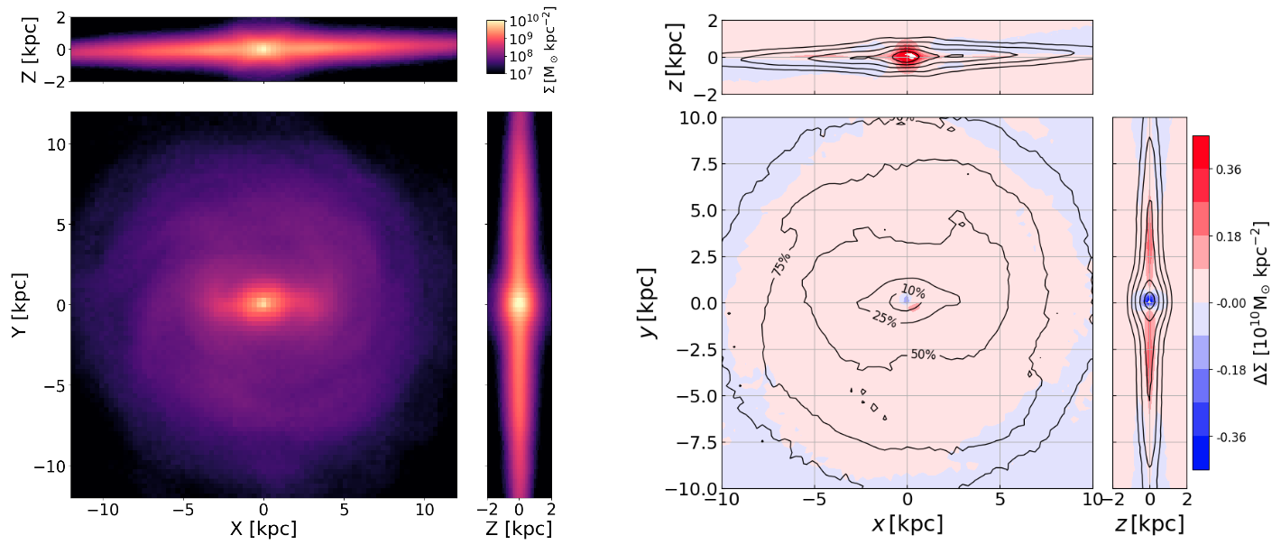
Figure 1: Left: Column density maps of the stellar distribution within our model, projected in the $xy$, $xz$ and $yz$ planes. Right: Residual column density maps of the stellar disc distribution within our model compared to S22, with contours representing cumulative fractions of the total stellar mass our model: $10\%,25\%,50\%,75\%,$ and $90\%$. This figure uses colour coding where red indicates a lack and blue denotes an excess of mass in our model, compared to the S22 analytic distribution.

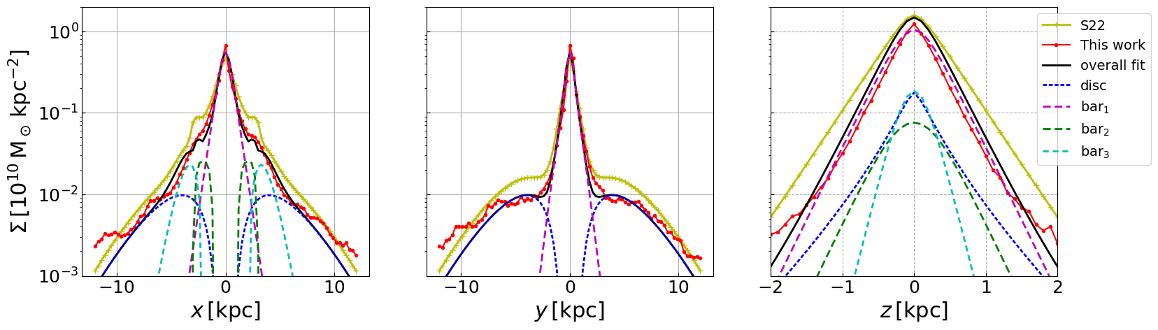
Figure 2: Stellar surface density profiles along the $x$ (left), $y$ (centre), and $z$ (right) axes of our model (red-dotted line) compared to the analytic Sormani et al. (2022) model (yellow-crossed line) including the overall best fit of an S22-type profile to our model (shown as a black solid line), and its various components represented by a distinct colour-coded dashed line: disc in dark blue, bar₁ in pink, bar₂ in green, and bar₃ (i.e. long bar) in light blue.

Here we explore the stellar density distribution in the inner galaxy of our numerical model (detailed in Section 2). In particular, we conduct a detailed examination of the stellar bar/bulge structure in our model, and compare these results against the characteristics of the stellar bar structure derived from observations of the inner Galaxy. For this comparison, we use the work of Sormani et al. (2022, hereafter S22), which presents an analytical description of the Milky Way’s stellar bar, based on the N-body model from Portail et al. (2017), developed to match observational data (e.g. Wegg & Gerhard, 2013; Wegg et al., 2015). The final analytical model from S22 is made out of four distinct components: an inner bulge/bar or X-shape structure (bar₁ and bar₂), a long bar (bar₃), and an axisymmetric disc. In Appendix A, we also include a further comparison with the stellar profiles of Ridley et al. (2017, hereafter R17), who use hydrodynamical simulations to model the dynamics of the Central Molecular Zone (CMZ) consistent with the observed gas flows within the inner Galaxy (including the $x_{2}$-type orbits). That model is able to reproduce the Inner Lindblad Resonances (ILR) and the barred galactic component, and hence also represents a good reference for the stellar profile in the Galactic Centre.

The left panel of Figure 1 shows the projected stellar surface density maps of our model across the three principal axes, where the bar is oriented along the $x$ axis. The right panel of this figure shows the residual map between our model, and S22’s analytical distribution. Figure 2 then shows 1D slices of the surface density of our model along the $x$, $y$ and $z$ axes (in red), alongside the profile from S22 (in yellow), and the best fit of an S22-type of profile to our model (in black). Details of this fitting can be found in Appendix A. While our model is almost always showing lower surface densities than the S22 analytic model, these discrepancies are not severe, with similar shapes for the distributions in the inner $\sim 5$ kpc, suggesting that our model can be adequately described with the same type of components - as shown by the black lines on Fig. 2. Notably, the largest differences are observed in the $z$-direction, where our model diverges most significantly from S22, showing discrepancies of up to $0.3$ dex in surface density, which suggest the surface density in our model can be up to a factor 2 lower. On the other hand, both $x$ and $y$ slices show a good agreement with the analytic model, specially within the $\pm 2$ kpc region. The deviations in those directions are less pronounced, where the surface density of our model is only $\sim 10-15\%$ lower than S22. The most substantial discrepancies in the $x$-direction primarily arise from the bar₂ component at $\sim 3$ kpc (see green curve on left panel of Fig. 2), whereas differences in the $y$-direction are predominantly due to the disc component in the $\sim 4-7$ kpc region (see blue curve on central panel of Fig. 2), although noting that this component is likely less accurate in S22.

Overall, we find that our model can be fit by a boxy/peanut bar component (bar_1,2 combined), with an approximate extension of $\sim 2$ kpc, and a long bar component (described by bar₃) with a half-length extension of $\sim 3$ kpc, which aligns well with both analytical models and other observations (e.g. Bissantz & Gerhard, 2002; Wegg & Gerhard, 2013). Generally, our model presents a thinner distribution than S22 and R17 models, with lower surface density within the inner $\sim 5$ kpc, and particularly so in the $z$-direction, where we find discrepancies of up to $0.3$ dex. A lower central mass could potentially impact the kinematics of the inner galaxy, which we will look into in the next Section.

3.2 Stellar Kinematics

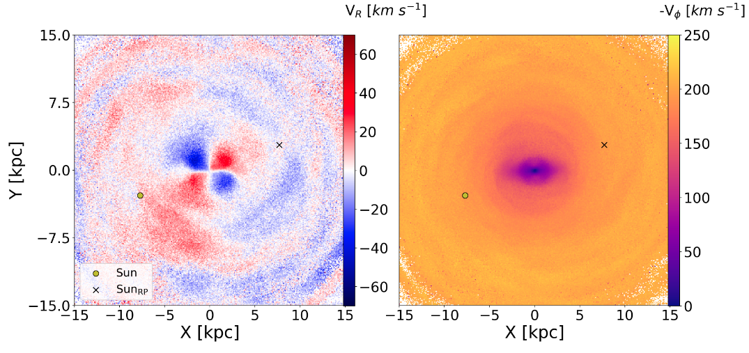
Figure 3: Top-view representations of radial ($V_{R}$, left panel) and the tangential ($-V_{\phi}$, right panel) velocity fields for the stellar component of our model. Note that $V_{\phi}$ is negative due to the clockwise rotation of the galaxy, and hence we plot the amplitude for clarity. The Sun is located at a viewing angle of $\phi_{\mathrm{obs}}=20^{\circ}$ with respect to the bar. Here we show the original Sun’s position as per the best viewing angle from Durán-Camacho et al. (2024), and the Sun’s reflection point (Sun_RP) at $180^{\circ}$ offset.

It is well known that the motions of stars and gas in galactic bars follow a quadrupole pattern, and this pattern has also been observed in the MW’s Galactic Centre (e.g. with Gaia DR2 and EDR3, Bovy et al., 2019; Queiroz et al., 2021). One of the sharpest views of this kinematical pattern was revealed by Gaia Collaboration et al. (2023), who analysed the kinematics of RGB and OB stars in the Milky Way using data from Gaia DR3. They found strong non-circular motions associated with this quadrupole pattern, with mean radial motions of the order of $\pm 40$ km s^-1. They also showed that streaming motions occur at larger Galactocentric radii ($R>5$ kpc), with possible association with Lindblad resonances. For the tangential component, they observed a clear elongated feature with lower tangential velocities along the bar’s major axis, within a $5$ kpc radius.

In order to benchmark our model against those observations, and understand how closely our model is able to replicate the kinematics of the centre of the MW, here we investigate the velocity fields associated with the bar pattern. In Fig. 3 we show the radial ($V_{R}$, left) and tangential ($-V_{\phi}$, right) velocities of our model’s stellar disc, up to a radius of $15$ kpc.

In this Figure, the bar is aligned with the $y=0$ axis, and we position the Sun at a distance of $8.275$ kpc from the galactic centre (GRAVITY Collaboration et al., 2021), and such that the galactic bar has an inclination angle of $\sim 20^{\circ}$ with respect to the observer, to match the results from Gaia Collaboration et al. (2023).

The radial velocity component in the left panel of Fig. 3 exhibits a quadrupole pattern within the long-bar extent, i.e. $\sim 5$ kpc from the galactic center. The radial velocities reach values of $\pm 45$ km s^-1, which is remarkably consistent with observed findings. As shown in the right panel of Fig. 3, the tangential velocity component also reveals an extended feature along the bar’s major axis with lower velocities, as expected, given that the stars are in $x_{1}$ orbits, with circular velocities closer to the bar pattern speed. For our model, those velocities are of the order of $\sim 40-70$ km s^-1 within the inner 5 kpc, which is similar to the observations.

As mentioned in Durán-Camacho et al. (2024), our simulation does not develop the $x_{2}$ orbits typically observed in the vicinity of the Central Molecular Zone, which has an extension of $\sim 250$ pc around the Galactic Centre (see e.g. Henshaw et al., 2016). These orbits are oriented perpendicular to the Galactic bar and are expected within the ILR for non-axisymmetric potentials (e.g. Contopoulos & Grosbol, 1989; Athanassoula, 1992). They emerge from the interplay between the bar’s dynamics and the stellar and mass profile of the bulge. These type of orbits may not develop if there is a lack of ILRs, a lack of mass in the inner regions (e.g. Hasan et al., 1993; Athanassoula et al., 2013), or the presence of a very strong bar potential (e.g. Contopoulos & Grosbol, 1989; Athanassoula, 1992). The existence of $x_{2}$ orbits is also sensitive to the pattern speed of the bar, which determines the position of the ILRs. Faster bars push the ILR inwards, while slower bars place the ILR farther out, allowing for a more extended $x_{2}$ region (see e.g. Athanassoula, 1992; Sellwood & Wilkinson, 1993). Given that our model’s pattern speed ($30\pm 0.2$ km s^-1 kpc^-1) is comparable to the observed values ($30-40$ km s^-1 kpc^-1, see e.g. Gaia Collaboration et al., 2023; Clarke & Gerhard, 2022), and that within our suite of models from Durán-Camacho et al. (2024), some of the simulations that do develop $x_{2}$ orbits have very similar pattern speeds ($29\pm 0.2$ km s^-1 kpc^-1), we conclude that the pattern speed is not the defining factor in this case. In addition, in Durán-Camacho et al. (2024), we demonstrated that our model does feature ILRs at $\sim$0.2 and $\sim$1.1 kpc, and thus that is not the reason the orbits do not develop.

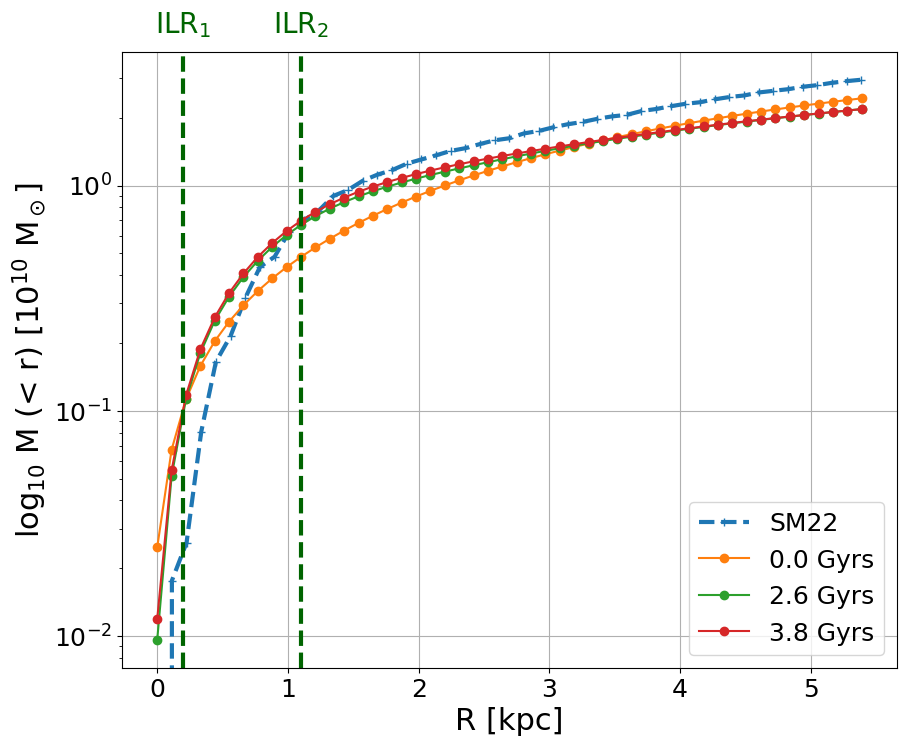
Figure 4: Spherical enclosed mass as a function of Galocentric radius for the analytical model from Sormani et al. (2022) (blue-dashed line), and our model at initial (orange-dotted line), optimal (green-dotted line), and late (red-dotted line) times. The position of the two ILRs in our model are shown as green vertical dashed lines.

A sufficiently high central mass concentration is known to contribute to the support of $x_{2}$ orbits (Athanassoula, 1992; Binney et al., 1991; Hasan et al., 1993). In order to understand if the lack of $x_{2}$ orbits in our model could indeed be a result of mass missing in the inner parts of the model (as potentially hinted by Sect. 3.1), here we investigate the total (spherically) enclosed stellar mass as a function of galactocentric radius $R$, for our model at different times, as well as the S22 analytical model (Fig.4)

This figure shows that, between the initial snapshot and the optimal time, there was some migration of mass towards the centre of the galaxy in our model, but that it stabilised at those values when compared to the later time. At these later times, when compared with the analytic profile, our model has, in fact, slightly greater mass in the central parts, with a discrepancy of only $\sim 3\%$ at the second ILR. As we move outwards, this trend reverses, where our model then starts to have lower enclosed masses compared to the analytic profile, but the difference is never larger than $7\%$ up to $5$ kpc.

In the previous section we found the largest discrepancies in the surface density distributions in the $z$ direction, and hence we also investigate the enclosed mass as a function of vertical direction $z$ (Appendix A). We find that in the mid-plane (within $|z|$ < 250 pc), our model is not missing any mass until well beyond the second IRL, and that indeed it is only at higher $z$ distances that the differences become noticeable. Given that $x_{2}$-type of orbits develop in the mid-plane (e.g. Athanassoula, 1992; Pichardo et al., 2002), it is unlikely that the lack of stellar mass in the inner galaxy of our models is the main contributing factor to the absence of these orbits. This is also corroborated by the fact that despite de similarities in the S22 and R17 stellar profiles for $R<2.5$ kpc, the hydrodynamical simulations from Portail et al. (2015) from which the S22 profile is based, also do not develop the $x_{2}$ orbits, while those from R17 do (see also Sormani et al., 2019; Tress et al., 2020).

An alternative explanation could thus be linked to the strength of the galactic bar itself. Athanassoula (1992) demonstrated that the prevalence of these orbits diminishes as the strength of the bar increases. Consequently, it could be that our model’s bar, by being effectively “narrower” than the observed one, might mean that the relative bar strength in our simulation is sufficiently high to suppress the formation of $x_{2}$-type orbits. It is possible that the inclusion of stellar and supernova feedback into these models will help steer up the dynamics of the gas and stars, and help diminish the relative strength of the bar potential - thus potentially facilitating the development of these $x_{2}$-type orbits. This will be investigated in follow up work.

In conclusion, despite the lack of the inner $x_{2}$-type orbits in our model (affecting the central $\sim$1 kpc), the overall density structure and kinematics of the inner regions of our simulation is close to the observed properties, making our model a suitable representation of the inner MW.

4 Galactic disc

Understanding the Milky Way’s spiral structure is central to interpreting its dynamical state and formation history, and yet there are significant uncertainties, particularly regarding the number, shape, and longevity of its spiral arms. In this section, we investigate the spiral pattern in the disc of our simulated galaxy by examining both the stellar and gaseous components. Following this, we focus on the solar neighbourhood, exploring how global spiral patterns manifest locally in stellar and gas kinematics.

4.1 Spiral pattern

As mentioned in Section 1, the configuration of the Milky Way’s spiral structure remains a subject of active debate. Whether our Galaxy is composed of a 2-armed, 4-armed, or more complex multi-armed pattern is still unclear. In this subsection, we investigate the spiral pattern in our model’s stars and gas, aiming to shed some light on the origin of observed inconsistencies in the Milky Way.

We use Fourier transformations for this purpose, as previously applied in nearby galaxies observations (e.g. Elmegreen et al., 1989; Rix & Zaritsky, 1995; Fuchs & Möllenhoff, 1999) and numerical simulations (e.g. Bottema, 2003). By decomposing the observed structures of the galaxy into their harmonic components, this method serves as an indicator of the multiplicity/periodicity of structures in a galactic disc. This method relies on the assumption that the galaxy’s spiral structure can be approximated by a periodic function in the azimuthal direction, with the Fourier coefficients providing a direct link to the underlying symmetry and number of arms. More details on this technique can be found in Appendix B.

The final representation of the Fourier amplitudes, $C_{n}$, of each Fourier coefficient (with harmonic number $n$), is shown in Fig. 5 as density plots across radial bins. The amplitude of each coefficient indicates the prominence of that type of multiplicity, and therefore, a prominent peak mode $n$ could be seen as directly linked to the dominant number $n$ of spiral arms at a given radius. However, as pointed out by Elmegreen et al. (1989), caution should be taken when interpreting the dominant mode as indicative of the exact number of spiral arms, as there is some degeneracy. As such, we use this Fourier decomposition as a means to inter-compare the multiplicity of the stellar and gaseous distributions, rather than to quantify their exact number of arms.

Figure 5: Density plots of the Fourier amplitudes ($C_{n}$) for each mode $n$ as a function of galactocentric radius, for stellar particles (top) and gas cells (bottom). The colour scale represents the amplitude, and therefore the strength of different spiral modes, with strong peaks indicating dominant spiral arms.

For the stellar component (Fig. 5, top panel), we find a dominant $n=2$ configuration extending up to $\sim 7$ kpc, with the highest amplitudes near the bar. Beyond $\sim 8$ kpc, the pattern weakens and transitions to multiple components as the stellar potential becomes more diffuse, with no particular dominant mode. This is also illustrated in Figure 6, where we show the dominant mode $n$ as a function of radius, and we can see that the stars maintain a dominant $n=2$ mode up to $\sim 7$ kpc before becoming more chaotic. These findings align with observations in external galaxies, where inner discs often show 2-arm structures, while outer regions display a more flocculent nature. We also detect a much weaker $n=4$ mode, which could be indicative of a 2+2 arm pattern, where two strong arms are accompanied by two weaker arms, consistent with Gaia studies suggesting a similar Milky Way structure (Poggio et al., 2021).

The gaseous component (Fig. 5, bottom panel) reveals a more complex picture. The gas exhibits no dominant mode over extended radii, highlighting its chaotic and transient nature under a live potential, indicative of a dynamic process of formation and destruction over time. This is also evident in Figure 6, where the dominant mode for the gas fluctuates almost randomly between $n=1-5$ inside $\sim 8$ kpc, with complexity increasing outward.

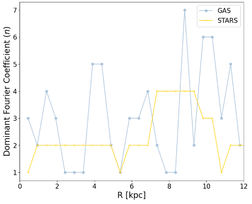
Figure 6: Dominant number of spiral arms as a function of galactic radius, obtained from the maximum Fourier coefficient (see Appendix B).

These findings are consistent with the complexity of the spiral patterns that we find when extracting the spiral arm ridges from the sharpened maps of the top-down stellar and gas surface densities (see Fig.15). The stellar spiral arms, are typically low contrast and smoother in nature (hence not being visually prominent in Figure 1), and we find $\sim 2-4$ arms in any radial cross section from 3 kpc up to 12 kpc. In the gas, however, the spiral pattern is sharper, which is consistent with observations of external galaxies, where spiral structure is often more apparent in the gas, dust, and young stars than in the old stellar disc (e.g. Elmegreen & Elmegreen, 1987; Elmegreen et al., 2011). That said, our model’s spiral arm ridges in the gas are significantly more numerous and segmented than the underlying stellar pattern. On average, we find $\sim 5-8$ ridges in any radial cross section from 3 kpc up to 12 kpc. In other words, we typically find twice as many spiral arm ridges in the gas than in the stars.

Overall, our model does not conform to a grand design spiral archetype. Instead, while a spiral pattern is always present, it is mostly transient, with the gas and stars often out of sync. This mirrors observations of external galaxies, where gaseous spirals display greater variability due to the interstellar medium’s dynamical response (see e.g. Elmegreen & Elmegreen, 1987; Maschmann et al., 2024; Dobbs & Bonnell, 2008; Renaud et al., 2013). Such hybrid behaviour highlights the diversity of spiral structures under evolving galactic conditions (Foyle et al., 2011; Hart et al., 2016).

As noted in Sect. 1.2, studies suggest the Milky Way shows both grand design and multi-armed features. For example, Drimmel & Spergel (2001) and Churchwell et al. (2009) found a two-arm structure in the inner Galaxy, while the outer disc is more complex. Spitzer GLIMPSE observations confirm this duality, showing dominant and fainter arms (Benjamin et al., 2005). Gas surveys (Nakanishi & Sofue, 2003; Kalberla & Kerp, 2009) also reveal significant variation, consistent with our model. This suggests that the Milky Way’s spiral structure may be inherently transient, with gas responding in a complex, non-density-wave-like manner, a point we explore further in the following sections (4.2 and 5.1).

4.2 Solar neighbourhood

The recent work by Khanna et al. (2023) has identified significant streaming motions for stars within $3.5$ kpc from the Sun, demonstrating tentative correlations between the velocity structures and the spiral arms. Using an axisymmetric model to subtract from the observed velocities, they quantified overall velocity trends and found that gradients in the radial and tangential components ($\Delta(-V_{\phi}$) and $\Delta V_{R}$) were not uniform, with variations averaging $\sim 5$ km s^-1 and $\sim 10$ km s^-1 respectively. However, the extent to which such velocity patterns can be related to the dynamics of the stellar and gaseous spiral pattern in the MW is incredibly hard to ascertain from observations. Indeed, as mentioned in Section 1.2, our knowledge of the position and extent of the stellar and gaseous arms remains highly uncertain, making these results tentative at best.

In order to shed some light into how the observed stellar kinematics pattern from Gaia may inform us of the underlying spiral arm structure and kinematics in the solar neighbourhood, here we investigate the equivalent stellar velocity patterns in our model, and then compare that to the underlying stellar and gaseous spiral pattern. For that, we obtain the velocity residuals in a similar way to the observations by Khanna et al. (2023) by contrasting the actual velocity fields observed in our simulation against an idealised rotation curve (see Appendix D for more details).

In Figure 7, we present the heliocentric velocity residuals, $\Delta(-V_{\phi})$ and $\Delta V_{R}$, for the data from the Gaia DR3 study by Khanna et al. (2023) (top), alongside our model’s stellar (middle) and gaseous (bottom) components within the mid-plane (|$z$| < 0.25 kpc). On the Gaia data maps we include the spiral arm tracks from Reid et al. (2019), and in the simulation panels, we have included the stellar and gaseous spiral arm ridges (in teal and black respectively), as identified using an unsharpening technique (see full details in Appendix C). From this Figure, we can see that the model’s gaseous spiral ridges loosely follow the tracks suggested by Reid et al. (2019), and that the general trends for the stellar kinematics in our model seem to be similar to those observed by Khanna et al. (2023), with both showing strong gradients in $\Delta(-V_{\phi})$ and $\Delta\mathrm{V}_{\mathrm{R}}$, albeit slightly more pronounced in the model, with magnitudes reaching as high as $15$ km s^-1 and $25$ km s^-1 for the tangential and radial components respectively. Overall, the stellar kinematics in our simulation show a relatively weak correlation with the positions of the spiral ridges (be those the gaseous or stellar arms), as none of the velocity components demonstrate a clear systematic alignment.

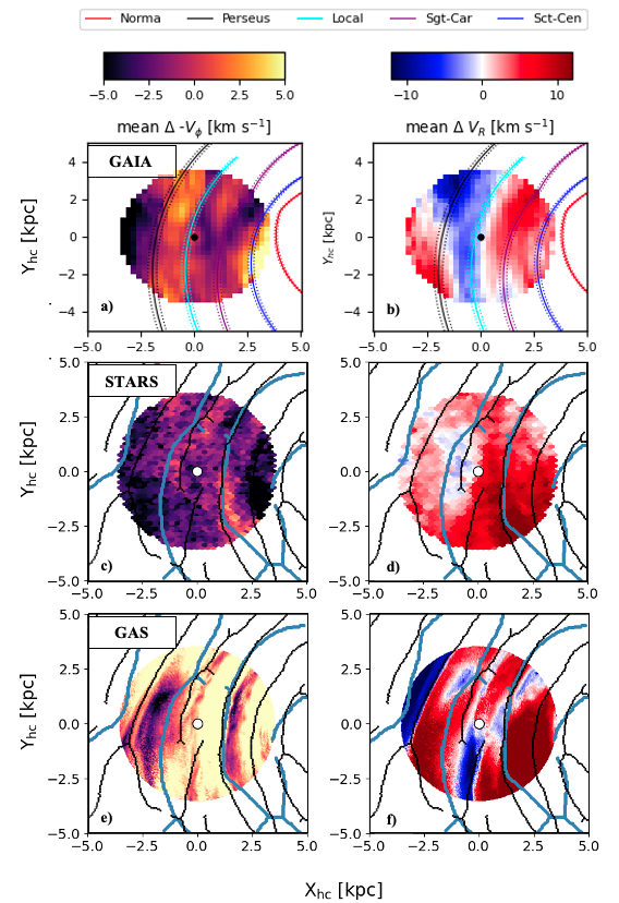
Figure 7: Heliocentric velocity residual maps for $\Delta(-V_{\phi})$ (left) and $\Delta V_{R}$ (right) for Gaia DR3 data from Khanna et al. (2023) (top), and our model’s stellar (middle) and gaseous (bottom) components in the galactic mid-plane (|$z$|< 0.25 kpc). The solid and dotted) lines on the top panels represent the gaseous spiral arm tracks from Reid et al. (2019). For our simulation, the stellar and gaseous spiral arm ridges extracted from the sharpened images of Fig. 15, are superimposed for comparison - gaseous arm ridges in black and stellar in teal. The galactic centre is outside this image, at (8.275,0) kpc.

When we look at the velocity pattern of the gas in our model, however, things are a bit different. Firstly, the amplitude of the velocity residuals are twice as large as those of the stars, reaching $\sim 30$ km s^-1 and $50$ km s^-1 for the tangential and radial components respectively. The velocity changes are also a lot sharper around the position of the gaseous spiral arms. Indeed we see that the circular velocities of the gas tend to be lower within (or close) to the gaseous spiral arm ridges, which suggests a deviation from the circular rotation curve induced by the acceleration towards the bottom of the potential well. When looking at the radial velocity component, we tend to see a number of gaseous spiral arm ridges at the convergence between inward and outward motions of the gas, which can help build up mass along the spiral arm ridges, thus conducive to spiral arm growth. There are, however, sections of spiral arms whose velocity pattern is no longer purely converging, and it is possible that those sections of spiral arms are in the process of dissolving.

In order to investigate how fast these kinematical patterns might change, we replicated our analysis by placing the observer at different locations and times (see Appendix D). The results from that exercise indicate a rapidly evolving system, with the velocity patterns changing in $\leq 10$ Myr, highlighting the transient nature of the observed streaming motions and spiral structures at any one time

In conclusion, our analysis shows that the pattern in the stellar structure and kinematics of our model at the chosen time is generally mild and consistent with Gaia observations of RGB stars, but that it translates into a gaseous pattern that is much sharper. This is also consistent with observations from Gaia Collaboration et al. (2023) who show that OB stars (which by being younger, are potentially better tracers of the underlying gas distribution that originated them) do align better with the gaseous spiral structures, specially towards the inner disc, but with low number densities their maps remain uncertain. Given the consistency between our results and MW observations, our model could therefore offer some insight into how the formation (and evolution) of the gaseous spiral structures of the MW, albeit potentially rapidly evolving, might be intricately inter-connected with the observed kinematics of the gas, and thus we explore this correlation further in the next section.

5 Correlation between kinematics and large-scale structures

Motivated by the fact that some of the sharp changes in the gas velocity patterns found in our model seem to be typically associated with the positions of gaseous spiral ridges, in this section we track the velocity changes both across, and along spiral arm segments, in order to identify what signatures are systematic, how they evolve with time, and explore the mechanisms driving gas accumulation and dispersal in the galactic disc.

5.1 Radial cross-sections of the galactic disc

In this section we investigate how the radial and tangential velocity variations relate to the gas surface densities, by looking at a radial cross-section of the galactic plane of our model. We define this cross-section by including all gaseous and stellar particles within the mid-plane of the galaxy (i.e. within $|z|<0.25$ kpc) and located within 50 pc of the line connecting the galactic centre and the Sun. Our analysis focuses on particles positioned to the left of the galactic centre (see white arrow on Fig. 17 of Appendix D).

Figure 8 shows the profile of the stellar and gaseous surface densities, followed by the tangential and radial velocity residuals along that cross-section. For all plots, we include the Sun’s position as a vertical dashed orange line, as well as the bar region as a shaded grey area. As our focus is on the dynamics in and around the over-densities of spiral arms, we will exclude this central (bar-dominated) region from our analysis.

From the top panel of Figure 8, we can see that the global stellar surface density (in yellow) shows a smooth decline with increasing galactocentric radius, while the cross-section (in black) shows more fluctuations. The comparison between the two aids the identification of the possible location of stellar over-densities (i.e. stellar spiral arms), although this shows that these are not very high-contrast features.

The second panel of Figure 8 shows that, unlike the stellar distribution, the gaseous spiral arms exhibit more pronounced overdensities, with up to six distinct arms identified as local peaks in the distribution, marked by red dashed vertical lines, with their approximate widths indicated by vertical red shaded areas. These arm positions are in good agreement with the spiral ridges used in Section 4.2 and defined in Appendix C. These spiral arms are overlaid on the subsequent panels, which display the velocity residuals distributions: tangential (blue) and radial (green).

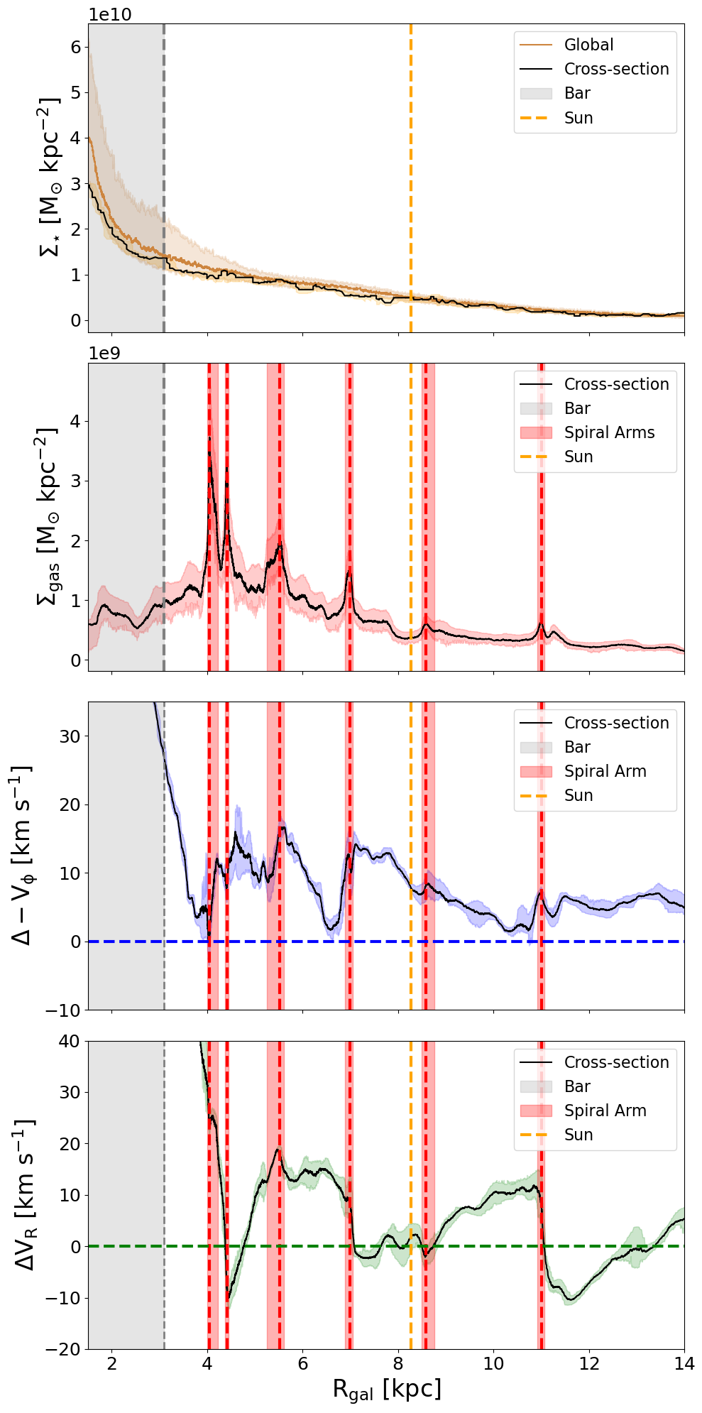
Figure 8: Surface density and velocity residuals of our model as a function of galactocentric radius for the stellar and gaseous components across the Sun’s line-of-sight with origin at the galactic centre. Panels show (top to bottom): stellar surface density, gas surface density, and tangential and radial gas velocity residuals. Running medians and interquartile ranges are shown for each of the distributions, with vertical shaded regions indicating the positions of the bar (grey) and spiral arms (red), and the solar position marked by a vertical orange dashed line.

From the tangential velocity residuals (third panel of Figure 8), we can see that the position of the spiral arms seem to be mostly associated areas of positive slope - i.e. where gas is moving slower in the inner side of the arm and faster in the outer side, effectively decreasing the differential rotation (and shear) within the arm. There are exceptions but typically related to lower gas surface density arm ridges. We can see that absolute values of these velocity residuals are larger ($\sim 10-15$ km s^-1) closer to the centre, where the spirals are also stronger and better defined, and these deviations decrease with distance.

The forth panel of Figure 8 shows the radial velocity component as a function of galactocentric radius. In this frame, a downward slope indicates regions where gas is radially converging, regardless of whether there is a change in sign from outward to inward motion, though the most significant convergence typically corresponds to a sign change. Conversely, an upward (positive) slope suggests divergence in the gas, and a flat slope indicates stable regions, where the gas is neither radially converging nor diverging, regardless of the direction or magnitude of the overall flow. Notably, there is a drop in velocities at the end of the bar region, indicating converging gas. The magnitude of this change ($\sim 40$ km s^-1) is much greater than the change in tangential residuals related to the bar ($\sim 15$ km s^-1), and it is at the end of this region of strongly converging gas that we find the strongest spiral arms in the gas surface density plot. For larger galactocentric distances along this slice, most gas exhibits relatively stable outwards motions, with the gaseous spiral arms appearing in converging regions where the slope in $\Delta V_{R}$ is negative, and in particular, where it shifts from positive to negative values. The larger radial velocity gradients across the identified spiral arms are of the order of $\sim 12-15$ km s^-1 kpc^-1. Conversely, clearly diverging regions (with positive slope) are typical of the inter-arm regions, although they have typically less steep slopes than the sharp changes found in spiral arms.

In order to test if these correlations are consistent across the galaxy, in Appendix E we also examine two more cross-sections positioned $\pm 20^{\circ}$ above (left) and below (right) the Sun’s line-of-sight (see Figure 19). We find that all trends are similar, with spiral arms typically associated with sharp negative slopes of $\Delta V_{R}$, and sharp positive slopes in $\Delta(-V_{\phi})$; while inter-arms show positive albeit very milder slopes in $\Delta V_{R}$.

Our analysis suggests that the position and strength of spiral arms strongly correlates with distinct velocity gradients in radial and tangential velocities. We also find that the strongest gaseous spiral arms, characterised by strongly converging gas, are mostly found in the inner galaxy, where the velocity changes are sharper, and partly driven (and sustained) by the bar. These results align with the findings of Urquhart et al. (2014), who highlight the prominence of the Sagittarius arm as a major gaseous feature in the Milky Way, based on observations of young massive stars from the Red MSX Source (RMS) survey. It remains to be seen, however, how persistent these velocity patterns are throughout time, which we explore in the following section.

5.2 Time-evolution of spiral arm segments

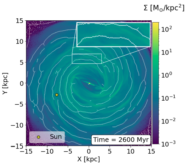
Figure 9: Top-down view of the stellar surface density distribution in the simulation at $t=2.6$ Gyr. The inset box shows the zoom in onto the spiral arm segment examined in detail in Section 5.2.

In this section, we use our model to explore the process of spiral arm growth and dissolution over time, and its link to the underlying kinematics.

We use the gaseous spiral ridge points (see Appendix C) to trace the underlying skeleton of the gaseous spiral structure, and follow the evolution of a selected spiral arm segment (see Fig. 9) over a period of $\sim 20$ Myrs. This particular region was chosen as an example of an arm with a section that is actively growing, and a section that breaks within this time frame (the time evolution of this spiral arm segment can be seen in Appendix F, Fig. 20).

We investigate the evolution of physical and kinematic conditions of the arm by tracking key quantities along the spiral ridge, namely the gas volume density ($\rho$), radial and tangential velocity residuals ($\Delta V_{\rm R}$ and $\Delta(-V_{\phi})$), and velocity divergence ($\nabla\cdot\mathbf{V}$). In addition, we also look at the fraction of dense gas ($f_{\rm dense}$) as the percentage of mass above a given volume density threshold (which we take to be $700~\mathrm{cm}^{-3}$ as the minimum density for gas with star-forming potential, in line with what is used for the insertion of sinks/star particles in similar galaxy-scale simulations, see e.g. Dobbs, 2015; Treß et al., 2021). The results are presented in Figure 10, where each column shows a different time (spaced by 5 Myrs). The two sections of the spiral arm which are growing (Section 1) and dispersing (Section 2) are shown as shaded grey areas.

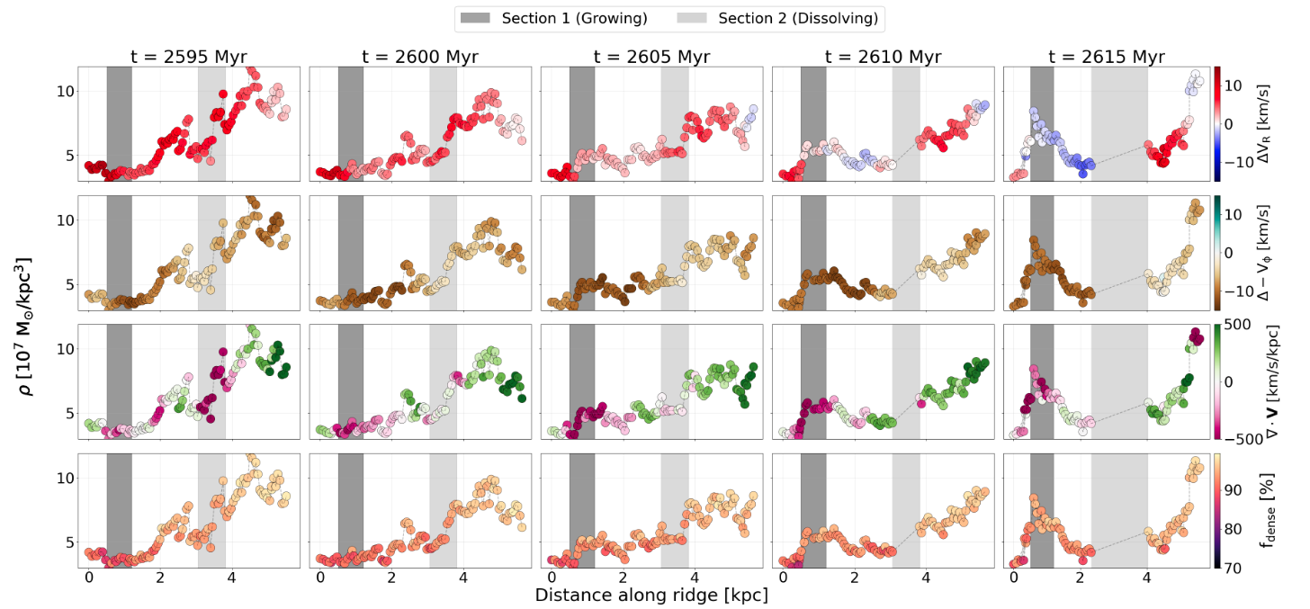
Figure 10: Time evolution of the volume density of the spiral arm segment selected in Figure 20 (Appendix F), shown as a function of distance along the spiral ridge. Each column represents a different snapshot, covering a 20 Myr period in 5 Myr intervals. The points are colour-coded (from top to bottom) by: (i) radial velocity residuals ($V_{R}$), (ii) tangential velocity residuals ($\Delta-V_{\phi}$), (iii) velocity divergence ($\nabla\cdot\mathbf{V}$), and (iv) the fraction of gas cells exceeding a critical volume density threshold of $700~\mathrm{cm}^{-3}$. Negative values of $\nabla\cdot\mathbf{V}$ indicate converging gas. The two spiral arm sections discussed in the main text, are highlighted with different shades of grey and tracked across all times as a visual guide.

Focusing on the arm section that is actively growing (Section 1), we can see that is starts with low densities, and mildly converging motions, and that as time progresses it becomes more convergent and densities increase considerably. This particular section exhibits a lower tangential velocity than the surrounding areas, which means the gas is slowing down in its rotation in this area, and therefore contributing to the gathering of material. This section also exhibits a very mild change of radial velocities along it, but given that the arm segment is near-perpendicular to the radial direction, this suggests this segment has a coherent “bulk motion”, with these radial velocity gradients only mildly reshaping the structure over time. That said, over the period of 20 Myr depicted here, this section evolves from having a bulk motion of mostly outward motions of $\sim 20$ km s^-1, to inward motions of $\sim-10$ km s^-1, highlighting the rapidly evolving nature of these kinematic patterns. In Fig. 20 we can further see that this particular section of the spiral arm ridge sits at the interface between an outward and inward motion, thus conducive to its growth.

In contrast, this behaviour is reversed in Section 2, where the arm breaks apart. Initially, the gas in this region has a high density peak and shows convergence, but over time it becomes progressively more divergent, eventually leading to the dissolution of the arm. This transition is also marked by a positive gradient in radial velocity residuals, as well as an increase of the tangential component, such that it is rotating faster in the leading part of this section, and hence the two ends of this section effectively feel a different “bulk motion” which contributes to pulling it apart. This process is accompanied by a redistribution of mass, as the volume density progressively decreases. Figure 20, on the bottom row, shows a more interesting perspective on this evolution: on the right-hand end of the arm ridge, the gas was initially converging (in pink) but then a green (diverging) valley appears and progressively splits the ridge into two fronts (one moving radially inwards, and another outwards).

Interestingly, this alternating convergence-to-divergence pattern within spiral arm ridges over time, is visible not just in this arm, but across the entire disc. Spiral arm ridges grow on convergence zones, at the interfaces between gas flows of opposing radial velocities, but after $20-40$ Myrs, the location of the once-dense ridges becomes divergent, as if the two shock fronts that formed it have now moved through each other. Spiral ridges thus split into two and continue travelling radially (one inward, one outwards) until they hit another front travelling in the opposite direction. Any given spiral arm seems to “survive” in its densest form for $<$ 20 Myrs before it splits, equivalent to the expected crossing time of the typical radial motions of the order of $\sim$20 km s^-1, for a spiral ridge of 400 pc width. This would suggest that the transient nature or the spiral pattern - their formation, survival, and reshaping - is intricately connected with the radial motions of the gas, a large portion of which are driven and sustained by the galactic bar and its butterfly pattern, which extends well into the galactic disc. This is obviously subject to this specific model, where we do not include self-gravity or feedback, and the lifetime of any given spiral ridge might be heavily affected by either of those factors considerably.

In summary, our combined analysis reveals a strong connection between the large-scale gas dynamics and the localised evolution of spiral arm segments in our galactic model. On global scales, peaks in the gas surface density trace the spiral arms and coincide with marked deviations in both radial and tangential velocity residuals. Gas tends to decelerate in their circular motion inside the arms, while radial velocity patterns highlight alternating converging and diverging flows at spiral arm locations. These large-scale features are consistent with previous N-body simulation results. For example, Kawata et al. (2014) found that gas around spiral arms exhibits sharp velocity variations, and Baba et al. (2013) showed that spiral arms form through swing amplification and dissolve due to dynamical forces. Our results illustrate the inter-linked and transient nature of spiral structures and gas dynamics. While a spiral pattern is always visible and distinct in the gas, any given spiral segment only survives as a single coherent feature for a few tens of Myrs, and this timescale is dictated by the amplitude of the radial motions present in the gas. Indeed, if this is the dominant mechanism by which arms grow and dissolve, then we might be able to infer the typical lifetime of spiral arms in the Milky Way, by measuring the amplitude of the gas radial motions. Of course the ability for a given gaseous spiral arm to grow and survive large-scale disruption in these dynamically evolving systems, might change if gas self-gravity and stellar feedback were to be included in our model, and we will explore this in future work.

6 Summary and Conclusion

In this work, we make use of the isothermal simulation presented in Durán-Camacho et al. (2024) as Model 4, chosen to provide a good representation of the overall observed Milky Way structure, and conduct an in-depth analysis of the structure and kinematical properties of both the stellar and gaseous components across various regions of that model galaxy. In particular, we investigate the influence of large-scale dynamics on defining the large-scale structures, as well as their potential impact on the agglomeration and disruption of gas, which in turn could set the initial conditions for the star formation processes. Our findings can be summarised as follows:

• The stellar distribution of our model’s inner galaxy (Section 3.1) can be well described by a boxy/peanut bar structure with a half-length of $\sim$2 kpc and a long bar component with a half-length of 3.1 kpc, aligning well with both analytical models and observational data of the Milky Way (Bissantz & Gerhard, 2002; Wegg et al., 2015; Sormani et al., 2022; Ridley et al., 2017). Nonetheless, the model exhibits a thinner surface density distribution within the inner 6 kpc, with the largest discrepancies in the vertical direction.

• The kinematic pattern of our model’s inner galaxy (Section 3.2) shows a radial velocity quadrupole pattern, and a tangential velocity deceleration region along the bar, both with similar extent and amplitude to the observations from Gaia (e.g. Gaia Collaboration et al., 2021a, 2023).

• Our model does not produce $x_{2}$ orbits in the inner-most regions ($<1$ kpc), and we explore if this could be due to a lack of central mass (Section 3.2). We find that the enclosed stellar mass within 5 kpc is only $\sim 7\%$ lower than that of other analytic models that reproduce the inner MW, but most of the discrepancies are for larger $z$ heights. In the mid-plane, the discrepancy within the ILRs (at $\sim$0.2 and 1.1,kpc) is negligible, suggesting that mass alone is not responsible for the absence of $x_{2}$ orbits. Instead, we argue that the strength of the bar and the lack of feedback likely play a more significant role in suppressing them. This hypothesis will be explored in future work.

• We examined the spiral structure of our model using Fourier decomposition and by extracting the spiral arm ridges from both the stellar and gas surface density maps (Section 4.1). Both analyses suggest that the gas shows sharper and more numerous spiral arm features throughout the disc than the stars, although neither component can be described by a well-defined number of spiral arms over extended radii, and the gas and stars are not necessarily synchronised in their spiral structure. These findings highlight that although a spiral structure is always present in both components it does not conform to a grand-design archetype. If taken as an analogue to the MW, this view of a more dynamically evolving spiral pattern in our model could explain the observational difficulty in determining the number of spiral arms in the MW.

• We analysed the stellar kinematics around the solar neighbourhood (Section 4.2) and compare to the observed stellar velocity distribution from Gaia DR3 (e.g. Khanna et al., 2023; Gaia Collaboration et al., 2023). We find our model to be largely in agreement with the observations (albeit with slightly larger amplitudes in the velocity residuals), but we find that there is not always a unique correlation between specific changes in the velocity of the stars and the position of the spiral arms (may those be the gas or stellar arms). However, we find that the gas experiences much shaper kinematic changes, in both radial and tangential directions, which correlate better with the position of the gaseous spiral arms.

• By analysing the specific changes of velocity along cross-sections of the disc (and therefore cross-sections of various spiral arms, see Section 5.1), we found systematic patterns associated with the position of strong gaseous spiral arms. In particular, we find they are regions of reduced differential rotation (seen as increasing tangential velocities from the inner to the outer side of the arm), and regions of strong radial velocity convergence.

• Our time-evolution study of a spiral arm segment (Section 5.2), suggests that these tangential and radial velocity patterns are rapidly evolving, and that this leads to the growth and dissolution of spiral arm segments in relatively short timescales ($<20$ Myrs). We find that arm growth is preceded by converging radial flows, coinciding with increases in volume density and in the fraction of gas above a critical density threshold for potential star formation. Conversely, arm destruction correlates with diverging flows and velocity gradients that shear the structure apart. These findings support a scenario in which the persistence of spiral arms is closely related to the large-scale kinematic environment and, in particular, the amplitude of radial motions - driven in large by the extended butterfly pattern induced by the galactic bar well into the galactic disc.

In conclusion, our findings reveal a transient nature of the spiral pattern in our model, challenging the traditional view of these structures as stable features in galaxies akin to the Milky Way, as predicted by the density wave theory. While our isothermal simulations do not include star formation, the observed gas dynamics suggest that spiral arms primarily act as mechanisms for gas accumulation, in a more complex and chaotic fashion than the typical grand-design spiral patterns. These fluctuating patterns indicate that the relationship between spiral arms and star formation is more complex and potentially less direct than previously assumed. This aligns with observational evidence, where the relationship between spiral arms and star formation is found to be complex and not always causal.

However, our model lacks self-gravity, chemistry, and stellar feedback mechanisms, factors likely to influence the star formation process itself, as well as the longevity and stability of spiral arms. Incorporating these physical processes in future simulations will help clarify whether gas accumulation in spiral arms under specific conditions is sufficient to initiate star formation, or whether additional environmental factors play a more dominant role. Despite these limitations, our work offers valuable insights into the processes shaping galaxies similar to the Milky Way and our model thus offers a basis for a more dynamic framework to study the formation and evolution of molecular clouds and stars, with potential further implications for the understanding of star formation in nearby galaxies.

Data Availability

The maps for the top-down surface density, velocity and lv projection of our best model have been made publicly available through the publication (Durán-Camacho et al., 2024), and can be found at the Following the Flow Of Gas in Galaxies (FFOGG) project website (https://ffogg.github.io/). Any data not available on the website can be provided upon requests to the authors. With this article, we further make available a video of the time evolution of the spiral structure of our simulation, with specific focus on the evolution of the different kinematical patterns studied here.

Appendix A Inner Galactic Stellar Profiles

In Section 3, we investigate the stellar surface density distribution in our model, and compare it to the work from Sormani et al. (2022, S22) and Ridley et al. (2017, R17). Here we provide more details on that comparison, as well as the fitting of the S22-type of profile to our model.

Sormani et al. (2022) presents an analytical model tailored to describe the stellar profile of the inner Galaxy, based on the N-body model from Portail et al. (2017), which had been developed to match observational data (e.g. Wegg & Gerhard, 2013; Wegg et al., 2015). Their global density profile (Eq. 1) includes 4 components: a boxy/peanut region in the centre which is described by the components bar_1,2, a long bar described by bar₃, and an axisymmetric disc.

$$\rho(x,y,z)=\rho_{\text{bar,1}}+\rho_{\text{bar,2}}+\rho_{\text{bar,3}}+\rho_{\text{disc}}$$ (1)

The profile for the first barred component is described by

$$\rho_{\text{bar,1}}(x,y,z)=\rho_{1}\,\text{sech}\left(a^{m}\right)\left[1+\alpha\left(e^{-a_{+}^{n}}+e^{-a_{-}^{n}}\right)\right]e^{-\left(\frac{r}{r_{\text{cut}}}\right)^{2}}$$ (2)

where

$$a=\left\{\left[\left(\frac{|x|}{x_{1}}\right)^{C_{L,1}}+\left(\frac{|y|}{y_{1}}\right)^{C_{L,1}}\right]^{\frac{C_{L,1}}{L}}+\left(\frac{|z|}{z_{1}}\right)^{C_{U,1}}\right\}^{\frac{1}{C_{U,1}}},$$ (3)

$$a_{\pm}=\left[\left(\frac{x\pm cz}{x_{c}}\right)^{2}+\left(\frac{y}{y_{c}}\right)^{2}\right]^{\frac{1}{2}},$$ (4)

$$r=\left(x^{2}+y^{2}+z^{2}\right)^{\frac{1}{2}}.$$ (5)

The profiles for barred components i $=\{2,3\}$ are given by

$$\rho_{\text{bar,i}}(x,y,z)=\rho_{i}\,e^{-a_{i}^{n_{i}}}\text{sech}^{2}\left(\frac{z}{z_{i}}\right)e^{-\left(\frac{R}{R_{\text{i,out}}}\right)^{n_{i,\text{out}}}}e^{-\left(\frac{R_{\text{i,in}}}{R}\right)^{n_{i,\text{in}}}},$$ (6)

where

$$a_{i}=\left\{\left[\left(\frac{|x|}{x_{i}}\right)^{C_{L,i}}+\left(\frac{|y|}{y_{i}}\right)^{C_{L,i}}\right]^{\frac{C_{L,i}}{L}}\right\}^{\frac{1}{C_{L,i}}},$$ (7)

$$R=\left(x^{2}+y^{2}\right)^{\frac{1}{2}}.$$ (8)

Finally, the galactic disc is represented with an axisymmetric profile as defined by

$$\rho_{\text{disc}}(R,z)=\frac{\Sigma_{0}}{4z_{d}}e^{-\left(\frac{R}{R_{d}}\right)^{n_{d}}}e^{-\frac{R_{\text{cut}}}{R}}\text{sech}\left(\frac{|z|}{z_{d}}\right)^{m_{d}},$$ (9)

where $R$ is the cylindrical radius from equation 8. We note however that their analytical model was produced by fitting data from the inner Galaxy, and hence this disc profile should not be taken as an accurate representation of the Milky Way’s disc beyond $\sim 4-5$ kpc.

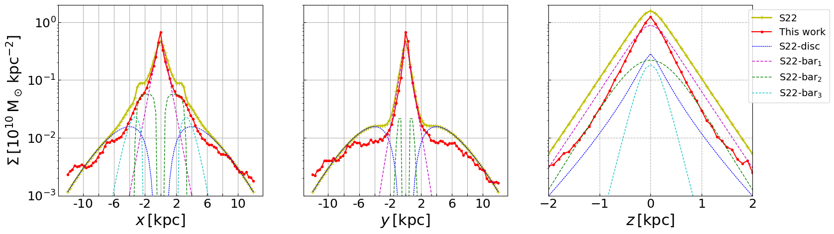
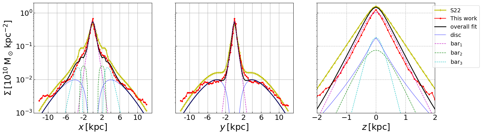
Figure 11: Stellar surface density along the $x$ (left), $y$ (middle), and $z$ (right) axes of our model compared to the Sormani et al. (2022) analytic model (S22). Top row shows the comparison between our model (red-dotted line) and the S22 model (yellow-crossed line). The different coloured-dashed lines represent the various galactic components of the S22 model: disc in dark blue, bar${1}$ in pink, bar${2}$ in green, and bar₃ or long bar in light blue. Bottom row includes the overall best fit of our model (black solid line) along with its components, represented by the same colour-coded dashed lines as in figures in the top row. Left-hand and middle panels correspond to the $x$ and $y$ axes in the ($x$,$y$) top-view map, while right-hand panels corresponds to the $z$-axis in the ($x$,$z$) map.

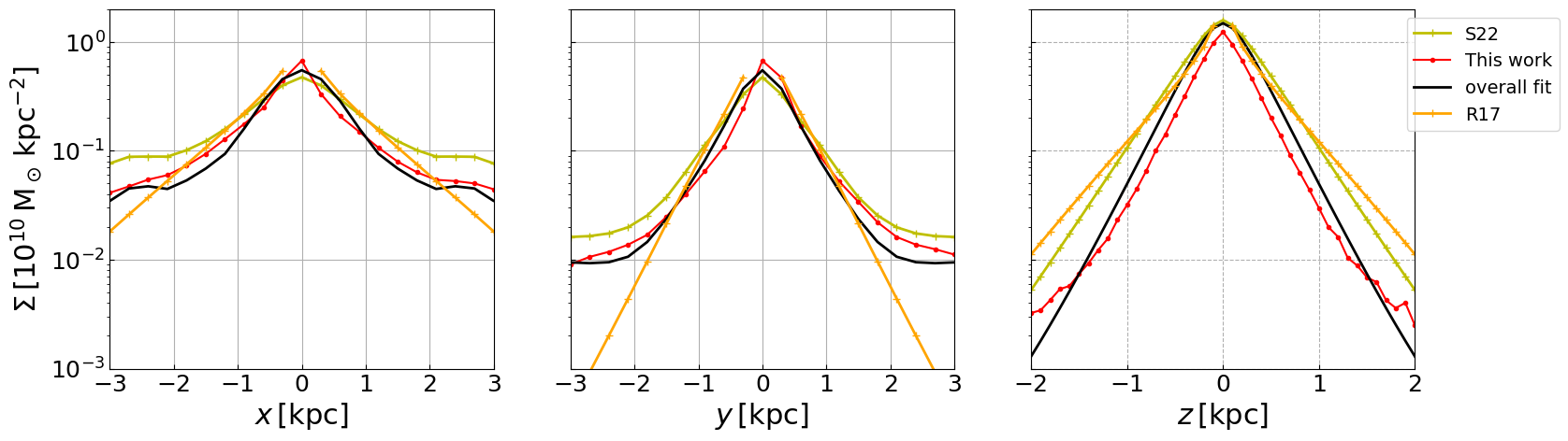
Figure 12: Similar to Fig. 2, zoomed-in to the $\pm 3$ kpc region in the $x$ and $y$ directions, and including the profile from R17 excluding the halo contribution (in orange), the S22 model in yellow, our model in red, and the S22-type profile fit to our model in black.

Table LABEL:table_2 shows the $27$ different parameters as adopted by S22, as well as the parameters which were further fitted to our model’s stellar distribution, using the same profiles. Note that the most notable differences of our fit compared to S22’s, are for the barred component 2 (which controls the inner bar’s boxy appearance), where both the size and peak surface densities are changed. Figure 11 shows the resulting 1D profiles of S22, when slicing the surface density images through through the 3 principal axis, as well as our model’s profile and respective fit.

Table 1: Best-fitting parameters for our numerical model, compared to the analytical model by Sormani et al. (2022). S22 values are shown only when they differ from this work.

Parameter	This work	S22	Units		Parameter	This work	S22	Units
Barred component 1					Disc
$\rho_{1}$	0.386	0.316	$10^{10}\mathrm{M}{\odot}\mathrm{kpc}^{-3}$		$\Sigma_{0}$	0.065	0.103	$10^{10}\mathrm{M}{\odot}\mathrm{kpc}^{-2}$
$x_{1}$	0.490	-	kpc		$R_{d}$	4.750	-	kpc
$y_{1}$	0.392	-	kpc		$z_{d}$	0.151	-	kpc
$z_{1}$	0.229	-	kpc		$R_{cut}$	4.690	-	kpc
$c_{||}$	1.991	-	–		$n_{d}$	1.540	-	–
$c_{\bot}$	2.232	-	–		$m_{d}$	0.716	-	–
$m$	0.975	0.873	–
$\alpha$	0.626	-	–
$n$	1.940	-	–
$c$	1.342	-	–
$x_{c}$	0.751	-	kpc
$y_{c}$	0.469	-	kpc
$r_{cut}$	4.370	-	kpc
Barred component 2					Barred component 3
$\rho_{2}$	0.028	0.050	$10^{10}\mathrm{M}{\odot}\mathrm{kpc}^{-3}$		$\rho_{3}$	1743.049	-	$10^{10}\mathrm{M}{\odot}\mathrm{kpc}^{-3}$
$x_{2}$	9.960	5.360	kpc		$x_{3}$	0.478	-	kpc
$y_{2}$	0.713	0.959	kpc		$y_{3}$	0.267	-	kpc
$z_{2}$	0.472	0.611	kpc		$z_{3}$	0.252	-	kpc
$n_{2}$	3.050	-	–		$n_{3}$	0.980	-	–
$c_{L,2}$	0.970	-	–		$c_{L,3}$	1.880	-	–
$R_{2,out}$	2.840	3.190	kpc		$R_{3,out}$	2.204	-	kpc
$R_{2,in}$	1.260	0.558	kpc		$R_{3,in}$	7.607	-	kpc
$n_{2,out}$	16.200	16.731	–		$n_{3,out}$	-27.291	-	–
$n_{2,in}$	7.160	3.196	–		$n_{3,in}$	1.630	-	–

We also compare our model with the hydrodynamical simulation presented in Ridley et al. (2017), which simulate the dynamics of CMZ, and is based on observations of NH₃ (1,1) emission from the HOPS survey and an improved potential from McMillan (2017). The R17 model includes 3-dimensional profiles for three components: bar, bulge, disc and halo. For the purpose of comparing the R17 model to our model’s stellar profile in the galactic centre alone, we exclude the halo component of R17, and confine our analysis to the inner 3 kpc, where that component is negligible.

Figure 12 shows the 1D surface density profiles of R17 compared to our work and S22, in that inner region. Overall, this figure echoes the results from the S22 comparison: the main discrepancies appear in the $z$-direction, where the R17 profile is even less steep than S22, suggesting a deficit in mass in our models in the vertical direction, which increases with distance from the mid-plane. This can be better visualised in the 2D residual maps between the projected stellar surface densities of our model and those of the S22 and R17 models (Fig. 13), where red/blue colours indicate a lack/excess of mass in our model, respectively. These plots reinforce the idea from the 1D analysis, that most of the discrepancy between our model and the two analytic descriptors (within the inner $\sim\,3$ kpc) is on the $z$-direction.

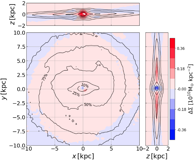
Figure 13: Residual column density maps of the stellar disc distribution within our model compared to two analytical models. The left panels show the comparison with the S22 analytical model, while the right panels compare with the analytical potential from R17. In both cases, the residuals are presented in the $xy$, $xz$, and $yz$ planes. Overlaid on the maps are contour plots representing cumulative fractions of the total stellar mass our model: $10\%,25\%,50\%,75\%,$ and $90\%$.

The above analysis focuses on the projected surface densities (in 1 and 2D), hinting at a potential lack of mass in our model in the inner regions, but in order to assess how significant this missing mass might be, and how it might affect the inner kinematics, we also investigated the differences in terms of 3D enclosed mass between our model, and S22. In Section 3.2, we presented the comparison of the spherically enclosed mass, but given that most of the disparities between our model and the analytic profiles were in the $z$-direction, here we include a comparison of the enclosed mass within different $z$ slices. Note that for this purpose we used the S22 profile, but the conclusions would be near identical if considering the R17 profile, given that they follow each other closely up to $R<2.5$ kpc and $|z|<1$ kpc.

Figure 14 shows the enclosed mass as a function of the cylindrical radius for each slice, and we can see that in the mid-plane slice (i.e. mid-slice), the enclosed mass in our model closely matches the analytical model up to $R\sim 2$ kpc, which is well past both ILRs. However, as we move outwards from the galactic mid-plane, our model presents an enclosed mass at the second ILR that is lower than the analytical model by 0.09 dex at intermediate $z$ (i.e. upper-slice) and 0.18 dex at higher $z$ (i.e. top-slice). This indicates that our model is more compacted in the mid-slice than the analytical model, with the mass concentration decreasing rapidly in the $z$-direction. We conclude, that although our model is indeed missing some mass in the inner galaxy, most of it is in the $z$-direction, and the differences in mass within the mid-plane of the galaxy are not significant enough to explain the lack of $x_{2}$-type of orbits.

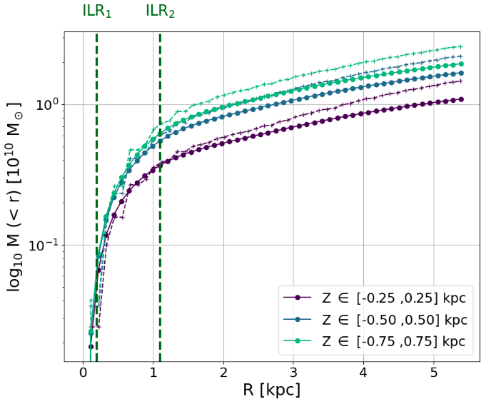
Figure 14: Cylindrical enclosed mass as a function of galactocentric radius for the analytical model from (Sormani et al., 2022) (cross-dashed lines), and our model (dot-solid lines). The different colours refer to the different $z$-slices: purple for the mid-slice ($0<|z|<0.25$ kpc), blue for the upper-slice ($0.25<|z|<0.5$ kpc) and green for the top-slice ($0.5<|z|<0.75$ kpc). The position of the two ILRs in our model are shown as green vertical dashed lines.

Appendix B The Basics of Fourier Series and Application to our model

An advantage of using numerical simulations for determining the number of spiral arms is that we have accurate positions for both the stellar and gaseous components, allowing us to apply techniques on the top-view column density distribution. This is otherwise challenging in observations of the Milky Way due to our inside view of the Galaxy. In order to have a better understanding of the spiral pattern present in our simulation, we use Fourier transformations, as studies of nearby galaxies (e.g. Fuchs & Möllenhoff, 1999) and numerical simulations (e.g. Bottema, 2003) have done in the past. We apply this technique to our model, both using gas and stars, to infer what spiral pattern emerges when using different tracers.

The Fourier Series provides a powerful method for approximating or representing a periodic function through a combination of simple harmonic functions (sine and cosine). This approach is particularly useful for decomposing complex waveforms into basic components, enabling a detailed analysis of structures such as the spiral arms of galaxies (e.g. Davis et al., 2012).

Fourier Series allow us to express a periodic function $f(x)$ with a period of $2L$ as a sum of sine and cosine functions. For a waveform $f(x)$ and a period $2L=\frac{2\pi}{k}$, where $k=\frac{\pi}{L}$, the spatial frequency $k$ relates to the wavelength $L$ of the periodic function. Consequently, for any integer $n$, the term $nkx=\frac{n\pi x}{L}$ specifies the harmonics of the function.

In this context, the Fourier coefficients — $a_{0}$ (the constant term), $A_{n}$ (the cosine coefficients), and $B_{n}$ (the sine coefficients) are determined through integration over the function’s period, as follows:

• The constant term $a_{0}$ is calculated as:

  $$a_{0}=\frac{1}{L}\int_{-L}^{L}f(x)\,dx$$

  This term represents the average or mean value of the function over one period.
  

• The cosine coefficients $A_{n}$ for $n=1,2,3,\ldots$ are given by:

  $$A_{n}=\frac{1}{L}\int_{-L}^{L}f(x)\cos\left(\frac{n\pi x}{L}\right)\,dx$$

  These coefficients measure the amplitude of the cosine components of the waveform, corresponding to the function’s "even" symmetry parts.
  

• The sine coefficients $B_{n}$ for $n=1,2,3,\ldots$ are determined as:

  $$B_{n}=\frac{1}{L}\int_{-L}^{L}f(x)\sin\left(\frac{n\pi x}{L}\right)\,dx$$

  These coefficients capture the amplitude of the sine components of the waveform, relating to the function’s "odd" symmetry parts.

The final form of $f(x)$ in terms of the Fourier coefficients $a_{0}$, $A_{n}$, and $B_{n}$ is given by the Fourier series expansion. This expansion expresses the periodic function $f(x)$ as a sum of its sinusoidal components:

$$f(x)=\frac{a_{0}}{2}+\sum_{n=1}^{\infty}\left[A_{n}\cos\left(\frac{n\pi x}{L}\right)+B_{n}\sin\left(\frac{n\pi x}{L}\right)\right]$$ (10)

We then proceed to identifying if there is a dominant periodicity mode in the sharpened images as a function of galactocentric distance via these Fourier coefficients. In our application, $f(x)$ represents the top-down surface density distribution of gas or stars within the simulation, where $x$ corresponds to the azimuthal angle in the plane of the galaxy, and $L$ relates to the radial extent of the region being analysed. The integer $n$ denotes the harmonic number and the resulting Fourier coefficients, $A_{n}$ and $B_{n}$, quantify the contribution of each harmonic $n$ to the overall Fourier coefficient at a given radius. The combined Fourier amplitude for each mode is given by:

$$C_{n}=\sqrt{A_{n}^{2}+B_{n}^{2}}$$ (11)

This amplitude $C_{n}$ indicates the strength of each mode. In essence, each radial bin’s density profile is approximated as a sum of these sinusoidal functions, with the coefficients indicating the presence and intensity of periodic patterns (e.g. spiral arms in our case). The process is repeated across multiple radial bins, and both sine and cosine coefficients (A_n and B_n) are calculated via numerical integration using the trapezium approximation. The integration is performed within defined radial bins of $0.6$ kpc separation, within a $15$ kpc radius. In Figure 5, we plot the resulting $C_{n}$ amplitude as a function of galactocentric radius and harmonic number $n$. For our analysis, we look at whether there is a clear dominant mode $n$ for periodicity at any given radial range, as that could be indicative of a preferred number ($n$) of spiral arms present in the simulation.

Appendix C Spiral ridges

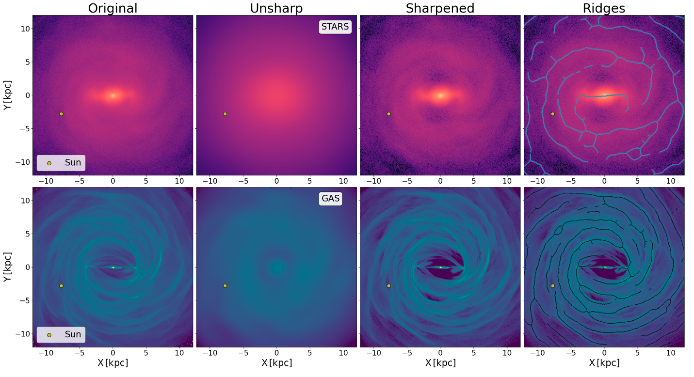
Figure 15: Maps illustrating the different steps involved in the unsharpening technique that we use to enhance the contrast of the spiral features from our model. From left to right: original, unsharp/smoothed, sharpened and spiral arm ridges images of the stellar (top) and gaseous (bottom) surface densities of our model. The galactic bar is positioned at the $y=0$ axis and the Sun’s position is marked with a yellow dot.

In order to investigate the link between the spiral arms and the kinematic pattern of our simulation, we extract the positions (or “ridges”) of the spiral arms. To do so, we use the top-down surface density images of the stars and gas, after applying an unsharp masking technique to enhance the visibility of high surface density features. This step is particularly needed for the stellar map, given their low-level contrast of spiral features in the original projection. This process involves taking the original image ($I_{\rm{orig}}$) and create a background (unsharp) image ($I_{\rm{bg}}$) that captures only the vary large-scale fluctuations. The final sharpened image ($I_{\rm{final}}$) is then obtained by doing $I_{\rm{final}}=I_{\rm{orig}}+a(I_{\rm{orig}}-I_{\rm{bg}})$, where $a$ is the factor that regulates the level of sharpening. In our case, we take $a=0.5$, and we produce $I_{\rm{bg}}$ by smoothing the original surface density maps with a Gaussian kernel of $2$ kpc. For the gas, however, because the central $\sim 0.15$ kpc radial region has much higher surface densities than the background, applying this kernel would overestimate the overall background in the central region. To avoid this, we first mask out this central high density region and then apply the $2$ kpc Gaussian kernel to the masked image, to produce the final unsharp map. The original, background and sharpened images from this procedure are shown in Fig. 15 (columns 1-3).

To extract the ridges of these sharpened images, we follow the technique described in Durán-Camacho et al. (2024), where we extracted the ’skeletons’ or footprints of the spiral arms from all l-v maps in our range of simulations. We provide here a brief description of this technique, but we refer the reader to the original work for further details on the methodology.

We start by slightly smoothing the sharpened images, by convolving with a small Gaussian smoothing kernel to ensure clarity and continuity in the arm structures. The kernel size was chosen based on the physical scale resolution we aim to investigate (in our case roughly of the order of a spiral arm width), and therefore we use a $\sigma=6$ pixels, which corresponds to 360 pc (i.e. FWHM of $\sim 850$ pc). We then compute the Hessian matrix of the image, with the respective eigenvalues, and create a binary mask of the image which traces the ridges of the map, by requiring the first eigenvalue to be negative (such that the surface is convex), with a stronger curvature than the second eigenvalue (to ensure that it is filamentary), and with an absolute value larger than a given threshold (to filter out the fainter structures). We then apply a binary erosion of $2$ pixels to this mask, in order to thinner the wider areas, and finally compute the medial axis of those eroded binary maps. The right-most column of Figure 15 shows the extracted stellar (top) and gaseous (bottom) ridges overplotted on the corresponding sharpened images.

Appendix D Heliocentric kinematic maps

In Section 4.2, we compare the stellar kinematics of our model with those observed with Gaia, as a means to infer whether our model sees the same type of kinematical patterns, and understand how much of that can inform us on the underlying stellar and gaseous spiral pattern. Here, we provide more details on how we produced the heliocentric maps from the model, and we explore how the results may vary as a function of time, and specific viewing angle.

In a similar way to the observations by Khanna et al. (2023), we obtain the velocity residuals by contrasting the actual velocity fields observed in our simulation against an idealised rotation curve. We compute the idealised rotation curve by assuming perfect circular rotation, with no radial ($V_{R}$) or vertical ($V_{z}$) velocities. We then consider the tangential velocity ($-V_{\phi,\mathrm{ideal}}$) as being the median velocity of all particles (stellar and gaseous) included in each radial bin. This idealised rotation curve can be seen in Fig. 16. We then obtain the velocity residual, $\Delta(-V_{\phi})$, by subtracting this idealised $-V_{\phi,\mathrm{ideal}}$ from the actual $-V_{\phi}$ observed for the particles within that segment. These residuals will identify non-circular motions and perturbations within the model. We focus our comparison on the trends seen on mid-plane of the galaxy (i.e. $0<z<0.25$ kpc).

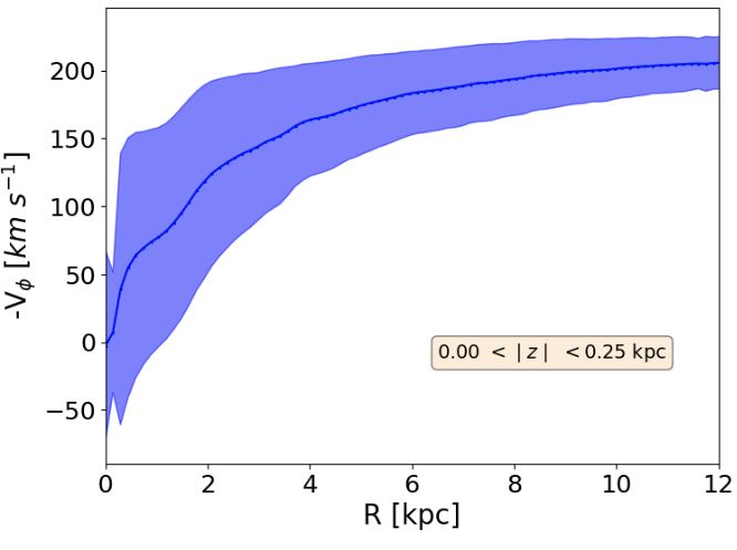
Figure 16: Median inverted tangential velocity ($-V_{\phi}$) as a function of radial distance from the galactic centre for the combined stellar and gaseous components within the mid-slice of our simulation. The shaded area corresponds to the standard deviation from the mean velocity value of all particles included within that radial bin.

In Figure 7, we presented the heliocentric velocity residuals, $\Delta(-V_{\phi})$ and $\Delta V_{R}$, for the data from the Gaia DR3 study by Khanna et al. (2023) (top), alongside our model’s. For that figure, we rotate our frame to match that used in the Gaia work, such that the $x$ axis is the line connecting the observer and the galactic centre, and the sun is at $(x,y)=(0,0)$, and we restricted our coverage and resolution of the stellar component to match that of Khanna et al. (2023) for a direct comparison. Here we include an extended version of our heliocentric velocity residual maps (Figure 17), covering up to 10 kpc in heliocentric distance, so that we cover the galactic centre (and thus comparable to the Gaia maps from Gaia Collaboration et al., 2023). In Figure 17, we also overlay, as arrows, the different cross-sections studied in Section 5.1 and Appendix E.

Between the Sun and the Galactic centre, the observations find predominantly radially-outward motions, and our model finds a similar trend for the stars inwards of the observer position. The observations also find that around the Local arm, there is a change of sign, and the stellar motions become predominantly inward motions for larger Galactocentric radii. Again, we find a similar trend in our model, albeit less sharp in amplitude. Intuitively, we would expect the convergence between the inward and outward motions to correspond to the position of the stellar spiral arm, but from our models, there is not always an obviously correlation between the velocity pattern of the stars, and the position of the stellar spiral arms.

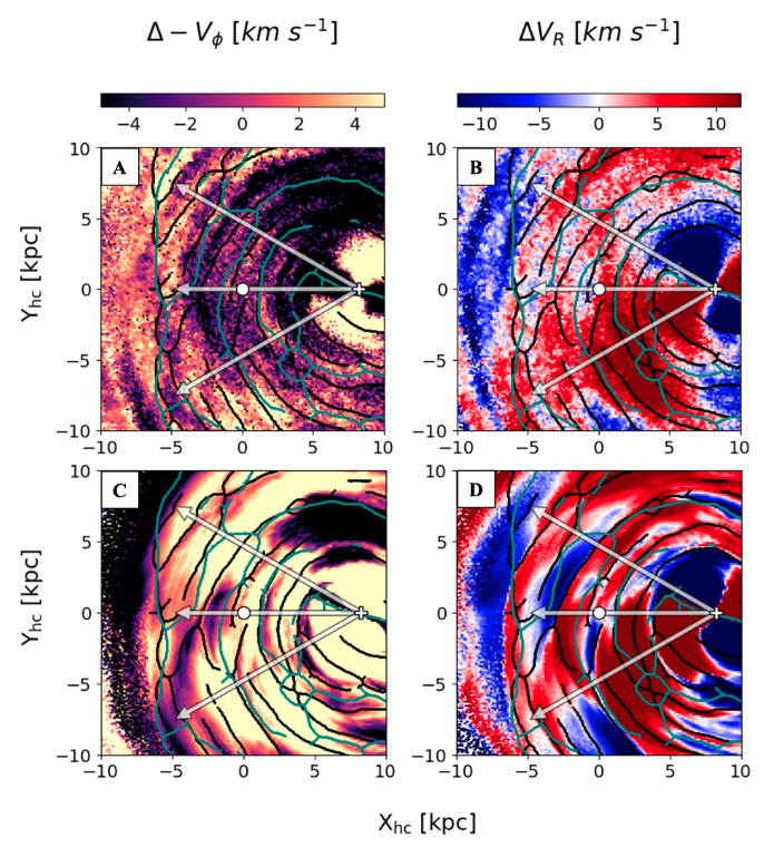
Figure 17: Heliocentric velocity residual maps for $\Delta(-V_{\phi})$ and $\Delta V_{R}$ (from left to right) for the stellar (top, A-B) and gaseous (bottom, C-D) components in the mid-slice of our model. The respective spiral arm ridges extracted from the sharpened images of Fig. 15, are superimposed for comparison - black for gaseous arms and teal for stellar arms. The Galactic Centre is depicted at (8.275,0) and marked with a white cross. The Sun’s position is marked with a white dot, and we restrict the $z$ component to the mid-plane ($|z|<0.25$ kpc). The different cross-sections studied in Section 5.1 are represented with white arrows.

Finally, in order to investigate how a different viewing angle and different times can alter the results from Section 3.2, in Fig. 18 we show the residual velocity maps around the solar neighbourhood for our model at two different times (10 Myr before and after the optimal time shown in Fig. 7), as well as for the Sun reflection point at the optimal time, Sun_RP (i.e. located at 180^∘ rotated around the galactic centre, such that the angle between the bar and the Sun_RP remains at 20^∘). This figure shows that the kinematical patterns (in particular changes of sign, or positions of maxima and minima) sometimes line up with the ridges of the stellar spiral arms and/or the gaseous ones, but there is no systematic trend. More interestingly, we can also see that these patterns seem to change quite rapidly: for instance, in a space of 20 Myr, the pattern of the radial velocities reverse such that, as we move from the outer galaxy through to the galactic centre, it goes from outflow-inflow (red-to-blue) 10 Myrs before, to inflow-outflow (blue-to-red) at the current time, to outflow-inflow again (red-to-blue) 10 Myrs after. The dynamic nature of these patterns is also nicely captured in a more detailed video of the time evolution of the system, available on the FFOGG website.

Overall, this exercise shows that our model - at the time and location as originally selected in Durán-Camacho et al. (2024) - successfully reproduces the kinematic imprints observed in the latest Gaia results, but it also underscores the rapid evolution of the kinematical pattern over time, and the difficulty in associating any given kinematical signature to the underlying presence of a spiral arm.

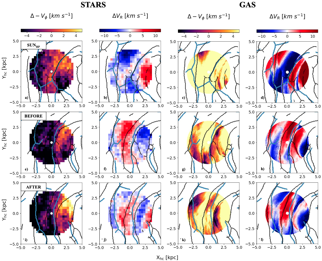
Figure 18: Top row shows the same as Fig.7, but with the observer positioned at Sun_RP (i.e. at the original observer’s position rotated by $180^{\circ}$) at the chosen optimal time. The first two columns present the tangential and radial velocity residuals for the stars, respectively, while the last two columns show the same for the gas. The second and third rows represent the model 10 Myr before and 10 Myr after the optimal time, respectively, keeping the observer at the original position (i.e. with $20^{\circ}$ inclination with respect to the bar). Spiral ridges, extracted from the respective sharpened images, are overplotted in black for the gaseous ridges and blue for the stellar ridges.

Appendix E Stellar and gaseous cross-sections

We present in Fig. 19 the analogous cross-sections to Fig. 8 positioned $\pm 20^{\circ}$ above (left) and below (right) the line connecting the galactic centre to the Sun. Similarly to the results shown in Section 5.1, for the cross-section going through the Sun, the stellar arm on the top two panels are faint and do not align with the gaseous spiral arms, and show weak correlation with the streaming motions in the residual velocities. There are a number of gaseous spiral segments identified along both directions. It is interesting to observe that the left column, corresponding to the $+20^{\circ}$ direction, aligns with the major axis of the galactic bar. This alignment explains why the tangential residuals in the bar region exhibit a positive slope starting from negative values, in contrast with the other two cases. This region intersects the strong negative feature seen along the major axis of the bar in the tangential residuals, as shown in Fig. 17 in Appendix D. Absolute changes within the bar region are of the order of $\sim 70$ km s^-1, while in the other direction they are $\sim 30$ km s^-1 across a radius of $\sim 3$ kpc. Beyond this point, similar trends are observed in both directions. Absolute changes in tangential and radial residuals are larger closer to the centre, where the gravitational potential is stronger and affected by the bar. Changes in tangential velocities across a spiral arm corresponds to a velocity gradient of $\sim 10$ km s^-1 kpc^-1, with gas generally decelerated within the spiral arm compared to the inter-arm region. Regarding radial residuals, converging points (downward slopes) occur within the spiral arms, while diverging points (upward slopes) are found in inter-arm regions. A notable example of diverging point can be seen in the bottom panel of the right column in Fig.19 at a distance of $\sim 10$ kpc. This area appears to be between two spiral arms and the gas in the inter-arm region diverges towards each arm, with a velocity gradient of $\sim 15$ km s^-1 kpc^-1.

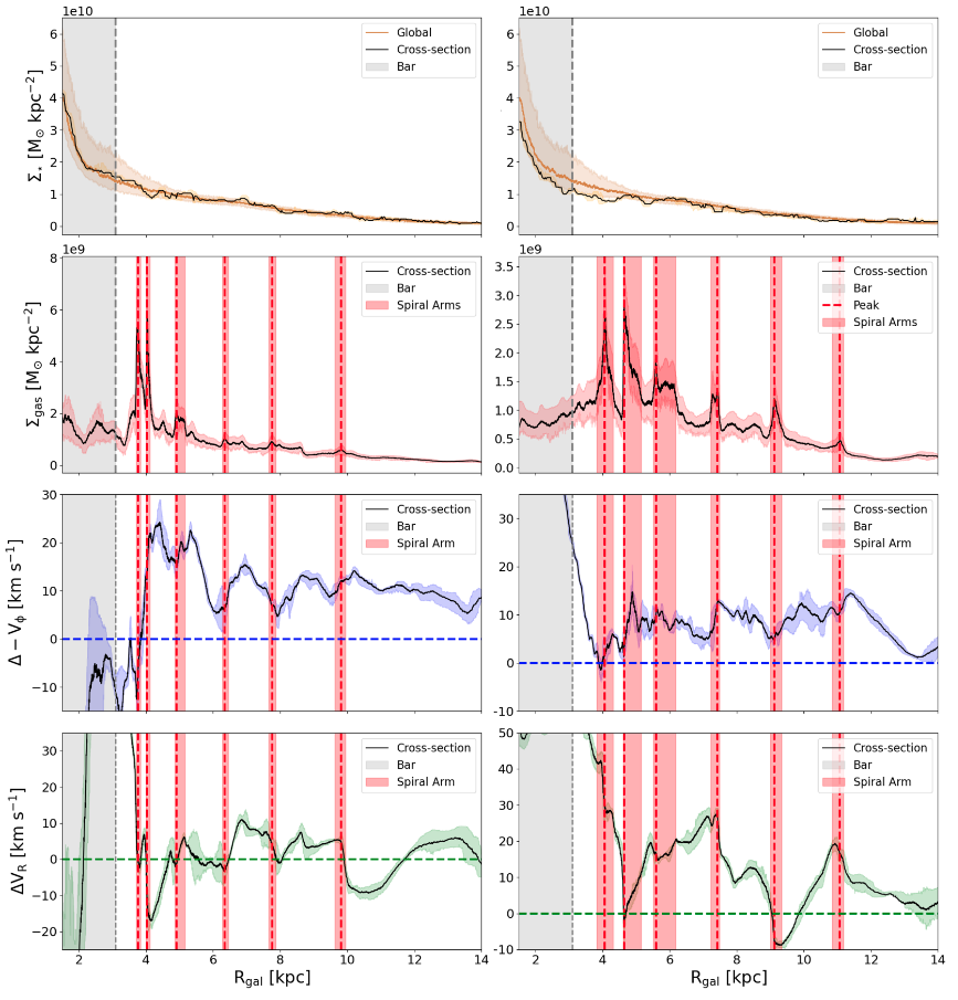
Figure 19: Same as Fig. 8, for a line-of-sight of $\pm 20^{\circ}$ (left, right respectively) from the Sun’s position with origin at the galactic centre. The galactic bar is aligned with the line-of-sight of left column.

Appendix F Spiral arm evolution across time

We examine the connection between spiral arm formation and dissolution and the large-scale kinematics in Section 5.2. To do this, we selected a specific spiral arm segment in the top-down view of the surface density distribution of our model and track its evolution over time. Figure 9 shows the surface density of the model at $t=2.6$ Gyr, highlighting the zoomed-in region corresponding to the selected spiral arm segment. Figure 20 shows the time evolution of this arm section, during $20$ Myr in timesteps of $5$ Myr represented with each column. From top to bottom, the rows display surface density, volume density, fraction of dense gas, radial and tangential velocity residuals, and the velocity divergence. We use these to then characterise the evolution of this spiral arm section by extracting different physical and kinematic properties along its ridge across multiple snapshots, as shown in Fig. 10.

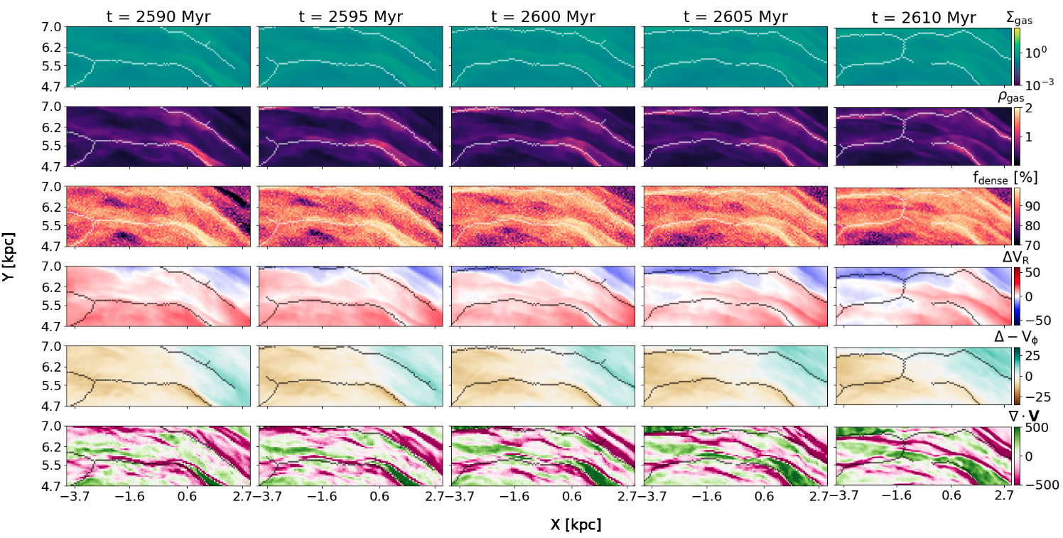
Figure 20: Time evolution of the spiral ridge analysed in Section 5.2 as a function of distance a long the ridge, shown for multiple time snapshots (columns). Each row corresponds to a different diagnostic map, from top to bottom: surface density, volume density, radial and tangential velocity residuals and velocity divergence. Coloured scatter points represent spiral ridge values obtained as explained in Appendix C.

In the first column of Fig. 20, we identify an arm segment, hereafter referred to as Segment 1, located near $x\sim-2.5\,\mathrm{kpc}$, where the spiral ridge is relatively faint. The bottom panel of this column shows that the gas in this segment is mildly converging, as indicated by a mild negative velocity divergence ($\nabla\cdot\mathbf{V}<0$), shown in light pink. This flow becomes more convergent over time, and leads to the growth of the spiral arm ridge, which reaches visibly higher surface (and volume) densities in the later snapshots (columns 4 and 5), $\sim 15-20$ Myr later. This convergence is also clearly visible in the radial velocities (fourth row), where at later times, this segment sits clearly at the interface between outflowing (red) and inflowing (blue) gas.

On the other side of this spiral arm section, we identified another segment (Segment 2), located near $x\sim 0\,\mathrm{kpc}$, which breaks/dissolves over this 20 Myr period. This ridge starts as a high density ridge with highly converging motions, but as time evolves, it becomes increasingly divergent and breaks apart. The bottom panels of this figure show that adjacent to the location of this spiral arm ridge, there is a highly divergent zone that develops and grows with time, effectively “splitting” and spreading this spiral arm segment into a wider - lower density - feature (as can be seen in the second row). The location of the arm in the first timestep is pushed downwards (following the lower edge of the split), while the upper edge is pushed outwards (and will eventually merge with the other visible spiral arm in the figure). This “opening” of the spiral arms is not just characteristic of this particular segment, but a recurring feature of the spiral arms in the simulation - best seen in the galaxy-wide time-evolution video available on the FFOGG webpage.

References

- Abbott et al. (2017) Abbott C. G., Valluri M., Shen J., Debattista V. P., 2017, MNRAS, 470, 1526
- Athanassoula (1992) Athanassoula E., 1992, MNRAS, 259, 328
- Athanassoula et al. (1983) Athanassoula E., Bienayme O., Martinet L., Pfenniger D., 1983, A&A, 127, 349
- Athanassoula et al. (2013) Athanassoula E., Machado R. E. G., Rodionov S. A., 2013, MNRAS, 429, 1949
- Baba et al. (2013) Baba J., Saitoh T. R., Wada K., 2013, ApJ, 763, 46
- Benjamin et al. (2005) Benjamin R. A., et al., 2005, ApJ, 630, L149
- Binney et al. (1991) Binney J., Gerhard O. E., Stark A. A., Bally J., Uchida K. I., 1991, MNRAS, 252, 210
- Bissantz & Gerhard (2002) Bissantz N., Gerhard O., 2002, MNRAS, 330, 591
- Bland-Hawthorn & Gerhard (2016) Bland-Hawthorn J., Gerhard O., 2016, ARA&A, 54, 529
- Blitz & Spergel (1991) Blitz L., Spergel D. N., 1991, ApJ, 379, 631
- Bottema (2003) Bottema R., 2003, MNRAS, 344, 358
- Bovy et al. (2019) Bovy J., Leung H. W., Hunt J. A. S., Mackereth J. T., García-Hernández D. A., Roman-Lopes A., 2019, MNRAS, 490, 4740
- Bureau & Freeman (1999) Bureau M., Freeman K. C., 1999, AJ, 118, 126
- Cabrera-Lavers et al. (2007) Cabrera-Lavers A., Hammersley P. L., González-Fernández C., López-Corredoira M., Garzón F., Mahoney T. J., 2007, A&A, 465, 825
- Churchwell et al. (2009) Churchwell E., et al., 2009, PASP, 121, 213
- Clark et al. (2019) Clark P. C., Glover S. C. O., Ragan S. E., Duarte-Cabral A., 2019, MNRAS, 486, 4622
- Clarke & Gerhard (2022) Clarke J. P., Gerhard O., 2022, MNRAS, 512, 2171
- Colombo et al. (2022) Colombo D., et al., 2022, A&A, 658, A54
- Contopoulos & Grosbol (1989) Contopoulos G., Grosbol P., 1989, A&ARv, 1, 261
- Contopoulos & Papayannopoulos (1980) Contopoulos G., Papayannopoulos T., 1980, A&A, 92, 33
- Dame et al. (2001) Dame T. M., Hartmann D., Thaddeus P., 2001, ApJ, 547, 792
- Davis et al. (2012) Davis B. L., Berrier J. C., Shields D. W., Kennefick J., Kennefick D., Seigar M. S., Lacy C. H. S., Puerari I., 2012, ApJS, 199, 33
- De Vaucouleurs (1964) De Vaucouleurs G., 1964, in Symposium-International Astronomical Union. pp 269–276
- Dobbs (2015) Dobbs C. L., 2015, MNRAS, 447, 3390
- Dobbs & Baba (2014) Dobbs C., Baba J., 2014, Publ. Astron. Soc. Australia, 31, e035
- Dobbs & Bonnell (2008) Dobbs C. L., Bonnell I. A., 2008, MNRAS, 385, 1893
- Dobbs & Pringle (2013) Dobbs C. L., Pringle J. E., 2013, MNRAS, 432, 653
- Drimmel (2000) Drimmel R., 2000, A&A, 358, L13
- Drimmel & Spergel (2001) Drimmel R., Spergel D. N., 2001, ApJ, 556, 181
- Duarte-Cabral et al. (2021) Duarte-Cabral A., et al., 2021, MNRAS, 500, 3027
- Durán-Camacho et al. (2024) Durán-Camacho E., et al., 2024, MNRAS, 532, 126
- Dwek et al. (1995) Dwek E., et al., 1995, ApJ, 445, 716
- Elmegreen & Elmegreen (1987) Elmegreen D. M., Elmegreen B. G., 1987, ApJ, 314, 3
- Elmegreen et al. (1989) Elmegreen B. G., Elmegreen D. M., Seiden P. E., 1989, ApJ, 343, 602
- Elmegreen et al. (2011) Elmegreen D. M., et al., 2011, ApJ, 737, 32
- Foyle et al. (2011) Foyle K., Rix H. W., Dobbs C. L., Leroy A. K., Walter F., 2011, ApJ, 735, 101
- Fuchs & Möllenhoff (1999) Fuchs B., Möllenhoff C., 1999, A&A, 352, L36
- GRAVITY Collaboration et al. (2021) GRAVITY Collaboration et al., 2021, A&A, 647, A59
- Gaia Collaboration et al. (2018) Gaia Collaboration et al., 2018, A&A, 616, A11
- Gaia Collaboration et al. (2021a) Gaia Collaboration et al., 2021a, A&A, 649, A1
- Gaia Collaboration et al. (2021b) Gaia Collaboration et al., 2021b, A&A, 649, A8
- Gaia Collaboration et al. (2023) Gaia Collaboration et al., 2023, A&A, 674, A37
- HI4PI Collaboration et al. (2016) HI4PI Collaboration et al., 2016, A&A, 594, A116
- Hammersley et al. (1994) Hammersley P. L., Garzon F., Mahoney T., Calbet X., 1994, MNRAS, 269, 753
- Hart et al. (2016) Hart R. E., et al., 2016, MNRAS, 461, 3663
- Hasan et al. (1993) Hasan H., Pfenniger D., Norman C., 1993, ApJ, 409, 91
- Henshaw et al. (2016) Henshaw J. D., et al., 2016, MNRAS, 457, 2675
- Hong et al. (2022) Hong T., Han J., Hou L., Gao X., Wang C., Wang T., 2022, Science China Physics, Mechanics, and Astronomy, 65, 129702
- Kalberla & Kerp (2009) Kalberla P. M. W., Kerp J., 2009, ARA&A, 47, 27
- Kawata et al. (2014) Kawata D., Hunt J. A. S., Grand R. J. J., Pasetto S., Cropper M., 2014, MNRAS, 443, 2757
- Khanna et al. (2023) Khanna S., Sharma S., Bland-Hawthorn J., Hayden M., 2023, MNRAS, 520, 5002
- Levine et al. (2006) Levine E. S., Blitz L., Heiles C., 2006, Science, 312, 1773
- Li et al. (2022) Li Z., Shen J., Gerhard O., Clarke J. P., 2022, ApJ, 925, 71
- López-Corredoira et al. (2005) López-Corredoira M., Cabrera-Lavers A., Gerhard O. E., 2005, A&A, 439, 107
- Majewski et al. (2017) Majewski S. R., et al., 2017, AJ, 154, 94
- Maschmann et al. (2024) Maschmann D., et al., 2024, arXiv e-prints, p. arXiv:2403.04901
- McMillan (2017) McMillan P. J., 2017, MNRAS, 465, 76
- Minniti et al. (2010) Minniti D., et al., 2010, New Astron., 15, 433
- Nakanishi & Sofue (2003) Nakanishi H., Sofue Y., 2003, PASJ, 55, 191
- Pettitt et al. (2020) Pettitt A. R., Dobbs C. L., Baba J., Colombo D., Duarte-Cabral A., Egusa F., Habe A., 2020, MNRAS, 498, 1159
- Pichardo et al. (2002) Pichardo B., Moreno E., Martos M., 2002, in Rosada M., Binette L., Arias L., eds, Astronomical Society of the Pacific Conference Series Vol. 282, Galaxies: the Third Dimension. p. 169
- Poggio et al. (2021) Poggio E., et al., 2021, A&A, 651, A104
- Portail et al. (2015) Portail M., Wegg C., Gerhard O., Martinez-Valpuesta I., 2015, MNRAS, 448, 713
- Portail et al. (2017) Portail M., Gerhard O., Wegg C., Ness M., 2017, MNRAS, 465, 1621
- Queiroz et al. (2021) Queiroz A. B. A., et al., 2021, A&A, 656, A156
- Ramón-Fox & Bonnell (2018) Ramón-Fox F. G., Bonnell I. A., 2018, MNRAS, 474, 2028
- Reid et al. (2019) Reid M. J., et al., 2019, ApJ, 885, 131
- Renaud et al. (2013) Renaud F., et al., 2013, MNRAS, 436, 1836
- Ridley et al. (2017) Ridley M. G. L., Sormani M. C., Treß R. G., Magorrian J., Klessen R. S., 2017, MNRAS, 469, 2251
- Rigby et al. (2016) Rigby A. J., et al., 2016, MNRAS, 456, 2885
- Rigby et al. (2019) Rigby A. J., et al., 2019, A&A, 632, A58
- Rix & Zaritsky (1995) Rix H.-W., Zaritsky D., 1995, ApJ, 447, 82
- Roman-Duval et al. (2010) Roman-Duval J., Jackson J. M., Heyer M., Rathborne J., Simon R., 2010, ApJ, 723, 492
- Sellwood & Carlberg (1984) Sellwood J. A., Carlberg R. G., 1984, ApJ, 282, 61
- Sellwood & Carlberg (2019) Sellwood J. A., Carlberg R. G., 2019, MNRAS, 489, 116
- Sellwood & Wilkinson (1993) Sellwood J. A., Wilkinson A., 1993, Reports on Progress in Physics, 56, 173
- Smith et al. (2020) Smith R. J., et al., 2020, MNRAS, 492, 1594
- Sormani et al. (2019) Sormani M. C., et al., 2019, MNRAS, 488, 4663
- Sormani et al. (2022) Sormani M. C., Gerhard O., Portail M., Vasiliev E., Clarke J., 2022, MNRAS, 514, L1
- Sparke & Sellwood (1987) Sparke L. S., Sellwood J. A., 1987, MNRAS, 225, 653
- Springel (2005) Springel V., 2005, MNRAS, 364, 1105
- Springel et al. (2005) Springel V., Di Matteo T., Hernquist L., 2005, MNRAS, 361, 776
- Stanek et al. (1994) Stanek K. Z., Mateo M., Udalski A., Szymanski M., Kaluzny J., Kubiak M., Krzeminski W., 1994, arXiv e-prints, pp astro–ph/9410044
- Tress et al. (2020) Tress R. G., Sormani M. C., Glover S. C. O., Klessen R. S., Battersby C. D., Clark P. C., Hatchfield H. P., Smith R. J., 2020, MNRAS, 499, 4455
- Treß et al. (2021) Treß R. G., Sormani M. C., Smith R. J., Glover S. C. O., Klessen R. S., Mac Low M.-M., Clark P., Duarte-Cabral A., 2021, MNRAS, 505, 5438
- Urquhart et al. (2014) Urquhart J. S., Figura C. C., Moore T. J. T., Hoare M. G., Lumsden S. L., Mottram J. C., Thompson M. A., Oudmaijer R. D., 2014, MNRAS, 437, 1791
- Valluri et al. (2016) Valluri M., Shen J., Abbott C., Debattista V. P., 2016, ApJ, 818, 141
- Wegg & Gerhard (2013) Wegg C., Gerhard O., 2013, MNRAS, 435, 1874
- Wegg et al. (2015) Wegg C., Gerhard O., Portail M., 2015, MNRAS, 450, 4050
- Weiland et al. (1994) Weiland J. L., et al., 1994, ApJ, 425, L81
- Weinberg (1992) Weinberg M. D., 1992, ApJ, 384, 81