Can Effective $4-$Quark Operators Describe Signals of a Supersymmetric Diquark Model at the LHC?

Abstract

The Standard Model Effective Field Theory (SMEFT) is constrained by current LHC data. Supposedly extensions of the Standard Model (SM) involving heavy particles can be constrained by matching onto the SMEFT. However, the reliability of these indirect constraints compared to those derived directly from the UV model remains an open question. In this paper, we investigate whether $4-$quark operators can accurately capture the effects of an $R-$parity-violating (RPV) supersymmetric model on the production of pairs of top quarks, for parameters that satisfy all known constraints and lead to measurable effects. We assume that the sbottom is the lightest supersymmetric particle and focus on its interaction with a light quark and a top quark; the sbottom thus acts like a specific diquark. The $4-$quark operators arise by integrating out the sbottom at tree level. We analyze measurements of inclusive top pair production by the CMS and ATLAS collaborations. We find that the $4-$quark operators can accurately describe the RPV model’s effects only for very heavy sbottom squarks, where the effects are well below the sensitivity of LHC experiments for all values of the RPV coupling that satisfy unitarity constraints. Therefore present or near-future bounds on this RPV model can not be derived from SMEFT analyses.

1 Introduction

More than 15 years after the LHC experiments started to take data they have not discovered a single particle not described by the Standard Model (SM). This is often seen as an argument against extensions of the SM that were designed to address the electroweak hierarchy problem by introducing new particles at the weak scale, e.g. by postulating that nature is supersymmetric (see e.g. Drees:2004jm ; Baer:2006rs ) or that additional spatial dimensions exist Antoniadis:1998ig ; Randall:1999ee .

Instead, a supposedly model–independent, or at least less model–dependent, approach has become popular in the last decade or so. Here one assumes that no new particles exist below the TeV scale. At energies well below a TeV effects of new particles can then be described by an effective theory (EFT), which extends the SM by a set of non–renormalizable higher–dimensional operators. EFTs of this kind had previously proven very helpful. For example, weak decays of charm– or beauty–flavored mesons and baryons can be described by a low–energy EFT which respects the $SU(3)_{C}\times U(1)_{\rm em}$ symmetry of the SM but describes $W$ and $Z$ exchange, as well as loops involving top quarks, through a set of higher–dimensional operators. Among other things, this simplifies the computation of QCD corrections (see e.g. Buchalla:1995vs ). Similarly, it is clear that baryon– and lepton–number violating interactions due to the exchange of gauge bosons predicted by Grand Unified theories (see e.g. Ross:1985ai ) can safely be described by an EFT at experimentally accessible energies Weinberg:1979sa .

These considerations led to the development of the Standard Model Effective Field Theory (SMEFT) Buchmuller:1985jz ; Grzadkowski:2010es ; Brivio:2017vri as a framework for systematically probing potential new physics beyond the Standard Model (BSM). It assumes that all interactions respect the full SM gauge symmetry, based on the group $SU(3)_{c}\times SU(2)_{L}\times U(1)_{Y}$. Since the SM already contains a sizable number of particles, well over $2,000$ new terms, with independent coefficients, can be constructed already at energy dimension $d=6$ if no further simplifying assumptions are made.

Phenomenological investigations of the SMEFT therefore have focused on relatively small subsets of these new operators. Examples are explorations of the top quark sector Buckley:2016cfg ; Buckley:2015lku ; Hartland:2019bjb ; Brivio:2019ius ; Ellis:2020unq ; Bissmann:2020mfi , Higgs and electroweak precision data Biekotter:2018ohn ; Ellis:2018gqa ; daSilvaAlmeida:2018iqo , gauge boson production Baglio:2020oqu ; Alioli:2018ljm ; Ethier:2021ydt ; Greljo:2017vvb , vector boson scattering Ethier:2021ydt ; Gomez-Ambrosio:2018pnl ; Dedes:2020xmo , as well as various low–energy constraints Aebischer:2018iyb ; Falkowski:2019xoe ; Falkowski:2017pss ; Bruggisser:2021duo . In the analysis of the top quark sector, the Minimal Flavor Violation (MFV) hypothesis DAmbrosio:2002vsn is usually adopted as the baseline scenario.

A rather ambitious more recent study Ethier:2021bye provides a global interpretation of Higgs, diboson, and top quark measurements from the LHC based on $50$ $d=6$ operators. By combining all input data, the individual and global $95\%$ confidence level intervals are obtained for all $50$ coefficients, using either linear or linear plus quadratic SMEFT calculations. “Linear” here means that only terms linear in the new Wilson coefficients are considered in the squared matrix element for any given process; such contributions occur if a SMEFT contribution interferes with an SM contribution. In contrast, a “linear plus quadratic” fit also includes terms bilinear or quadratic in the new Wilson coefficients. This gives sensitivity to contributions that do not interfere with the SM, e.g. to new color structures. However, these “quadratic” terms are ${\cal O}(\Lambda^{-4})$, i.e. they show the same dependence on the “new physics” energy scale $\Lambda$ as contributions that are linear in the Wilson coefficients of $d=8$ operators. Since the latter are not considered in the fit, a quadratic $d=6$ fit is not consistent from a power counting point of view.

One of the arguments in favor of SMEFT fits is that they should allow to directly read off constraints on the parameters of renormalizable models that predict new, heavy particles. To this end one only needs to match the model to the SMEFT, in order to establish the relations between the masses of couplings of the new particles proposed in a given model and the relevant SMEFT coefficients. Bounds on the latter then directly translate into bounds on the model parameters. This sounds straightforward; however, in practice this procedure may fail for a variety of reasons:

• Tree–level matching to the SMEFT basically amounts to shrinking propagators of new, heavy particles to a point. This can only work if the absolute value of the squared momentum flowing through this propagator is much smaller than the squared mass of the exchanged particle. This needs to be true in all events considered. At $e^{+}e^{-}$ colliders this will be true if the total Mandelstam$-s$ is much smaller than the squared mass $M^{2}$ of the new exchange particle, i.e. this criterion should be satisfied as long as $\sqrt{s}\leq 3M$. Of course, this statement also holds for $pp$ or $p\bar{p}$ colliders, if $\sqrt{s}$ is the hadronic center–of–mass (cms) energy. However, when writing the SMEFT Wilson coefficients as $1/\Lambda_{i}^{2}$, fits of current LHC data typically lead to bounds on the $\Lambda_{i}$ not much above $1$ TeV; energies of this order of magnitude can easily be reached even in the partonic cms. It is therefore not clear a priori whether the SMEFT approximation is indeed applicable for values of the $\Lambda_{i}$ near present or even future LHC sensitivity.

• A concrete renormalizable model will in general only generate a subset of SMEFT operators, at least at tree level. Moreover, it may impose relations between the SMEFT Wilson coefficients. This means that a global SMEFT fit, which allows (many) more operators than are actually generated by a given model, will usually lead to (much) weaker constraints on the coefficients of the operators that actually are generated, since the many parameter SMEFT fit allows for cancellations that may not be possible in any given model. This is true even if one finds a SMEFT fit that only considers the operators that are generated in the model of interest, unless the SMEFT fit also imposes the relations between the coefficients of these operators that follow for the given model. Since there’s in principle an uncountable infinity of such relations. This combinatorial problem means that in practice one will (almost) never find a SMEFT fit that actually has the right number of degrees of freedom to describe a given UV complete model. This difficulty arises also in analyses of data from $e^{+}e^{-}$ colliders, where annihilation events have an (almost) fixed center–of–mass energy (barring events with hard initial state radiation).

• A model may not generate any $d=6$ SMEFT operators at tree level; examples include supersymmetric models with conserved $R-$parity, and extra dimensional models with conserved KK parity. The actual LHC constraints on such models nearly always come from searches for the production of pairs of new particles; these constraints cannot be captured by SMEFT analyses.

Very similar problems were encountered when, several years before the SMEFT, a “WIMP effective theory” was suggested Bai:2010hh ; Beltran:2010ww aiming for a “model-–independent” description of monojet (and, more generally, “mono$-X$”) searches at the Tevatron and LHC. However, it became clear after a while that most UV–complete theories describing WIMP production at hadron colliders cannot be described by an effective field theory in the experimentally accessible parameter space. Instead, the real bounds typically come from searches for the on–shell production of the relevant mediator(s); see e.g. Fox:2011pm ; Goodman:2011jq ; Belwal:2017nkw ; Drees:2019iex

In this paper, we study the validity of the SMEFT description of an $R-$parity violating (RPV) supersymmetric model Barbier:2004ez . Specifically, we analyze measurements of inclusive top pair events, where the new particle contributes at tree level.

The RPV model is a simple extension of the minimal supersymmetrized standard model (MSSM) by adding extra superpotential terms that break baryon or lepton number (but not both, since that would lead to rapid proton decay). Searches for superparticles in the framework of this model have been carried out by both the ATLAS and CMS collaborations ATLAS:2021fbt ; ATLAS:2020wgq ; ATLAS:2019fag ; ATLAS:2018umm ; CMS:2021knz ; CMS:2018skt ; CMS:2017szl ; CMS:2016vuw ; CMS:2016zgb ; CMS:2013pkf ; ATLAS:2015gky ; ATLAS:2015rul . Here we consider a scenario where the superpartner of the right–handed $b$ quark, dubbed $\tilde{b}_{R}$, couples to a top quark and a light quark through a baryon number violating interaction. For simplicity we assume that all other superpartners are considerably heavier than $\tilde{b}_{R}$, so that their effect on LHC physics is negligible. Our model can thus be considered to be a particular example of a diquark model. By integrating out $\tilde{b}_{R}$ some $4-$quark operators are generated; of course, these operators are part of the SMEFT set.

Our main goal is to find out whether the SMEFT description in terms of these $4-$quark operators can provide reliable constraints on the RPV model through the analysis of inclusive top pair events. As mentioned above, a SMEFT description should indeed become possible for sufficiently heavy $\tilde{b}_{R}$. However, it is a priori not clear whether this is true for $\tilde{b}_{R}$ masses and couplings near present or near–future sensitivity; note that the relevant coupling is bounded from above by independent (theoretical) arguments.

In this RPV model new contributions to inclusive top pair production primarily arise from two sources: top pair production via sbottom exchange in the $t-$channel, as well as top pair plus single jet production from diagrams with a potentially on–shell sbottom in the intermediate state. We will see that in the latter case the $\tilde{b}_{R}$ tends to be produced on–shell even for masses up to $3$ TeV (with coupling around 1); this contribution cannot be described by the SMEFT. Nevertheless the SMEFT might still work for inclusive $t\bar{t}$ production, if this second contribution is small. Conversely, even if this contribution is small, some minimal sbottom mass is required for the first contribution to be described accurately by the SMEFT; only in this case will the limits derived within SMEFT be applicable to the RPV model.

The remainder of this paper is structured as follows. In Sec. 2 we review the theoretical framework of the RPV model and investigate its tree–level matching to $4-$quark operators. In Sec. 3 we briefly discuss the search for the production of on–shell $\tilde{b}_{R}$ squarks. In Sec. 4 we perform a detailed comparison between the RPV model and $4-$quark operators in terms of differential distributions and the resulting constraints derived from the measurements of inclusive top pair events from CMS and ATLAS. Finally we present our conclusions in Sec. 5.

2 Theoretical framework

If $R-$parity is not imposed the superpotential of the minimal supersymmetric standard model (MSSM) can contain the baryon number ($B$) violating terms Barbier:2004ez ,

$$W_{\not R_{p}}=\frac{1}{2}\sum_{i,j,k}\lambda_{ijk}^{\prime\prime}U_{i}^{c}D_{j}^{c}D_{k}^{c}\,,$$ (1)

where $i$,$j$,$k$ are generation indices. $SU(3)$ gauge invariance enforces antisymmetry of the coupling, $\lambda^{\prime\prime}_{ijk}=-\lambda^{\prime\prime}_{ikj}$. The corresponding piece of the Lagrangian is

$$\mathcal{L}_{U_{i}^{c}D_{j}^{c}D_{k}^{c}}=-\frac{1}{2}\sum_{i,j,k}\lambda^{\prime\prime}_{ijk}\left(\tilde{u}_{iR}^{\star}\bar{d}_{jR}d_{kL}^{c}+\tilde{d}_{kR}^{\star}\bar{u}_{iR}d_{jL}^{c}+\tilde{d}_{jR}^{\star}\bar{u}_{iR}d_{kL}^{c}\right)+\text{ h.c. }\,.$$ (2)

We are interested in inclusive top pair production at the LHC. The Lagrangian (2) can contribute to this via terms coupling a light quark, a top quark and some right–handed down–type squark. In order to maximize this contribution we want the light quark to be a $d_{R}$ (rather than $s_{R}$, which has considerably smaller parton density in the proton). In order to minimize $R-$parity conserving production of the intermediate squark via the exchange of a gaugino in the $t-$ or $u-$channel we select $\tilde{b}_{R}$ as exchanged squark. The relevant term in eq.(2) is thus the one proportional to $\lambda^{\prime\prime}_{313}$. Moreover, we assume that all other superparticles are considerably heavier than the right–handed sbottom, and hence play no role for LHC physics. It should be mentioned that assuming a single scalar superparticle to be much lighter than all the others isn’t very natural from the model building point of view; for example, larger gaugino masses can easily turn the squared mass of the scalar particle negative at only slightly larger energy scales. However, introducing additional relatively light particles would make it less likely that the scenario can be described by the SMEFT.

In order to keep things simple we also assume that $\lambda^{\prime\prime}_{313}$ is the only sizable new coupling. This also relaxes some constraints. For example, the measurements of flavor changing neutral currents (FCNC), e.g. in meson mixing, generally impose constraints on the products of two different RPV couplings Barbier:2004ez . Furthermore, neutron–antineutron oscillations are suppressed if gauginos are very heavy Barbier:2004ez ; calibbi2017baryonnumberviolationsupersymmetry . The remaining constraint on $\lambda^{\prime\prime}_{313}$ arises from perturbative unitarity, which requires that the coupling remains perturbative up to some large energy scale $M_{X}$,

$$\frac{\left(\lambda^{\prime\prime}_{313}\right)^{2}(M_{X})}{(4\pi)^{2}}<1\,.$$ (3)

In our case, setting $M_{X}\simeq 2\cdot 10^{16}$ GeV (the scale of supersymmetric Grand Unification), this requirement leads to Barbier:2004ez

$$\lambda^{\prime\prime}_{313}(1\ {\rm TeV})<1.12\,,$$ (4)

almost independently of the other parameters of the theory. This constraint implies that our RPV coupling cannot be larger than the $SU(3)$ gauge coupling.

Since this is quite a strong restriction, we also consider the weaker constraint from the requirement that the $\tilde{b}_{R}$ decay width does not become too large, which would jeopardize the validity of perturbation theory at the LHC energy scale. In our scenario the sbottom decays only into a top antiquark and a down antiquark, with decay width

$$\Gamma_{\tilde{b}}=\frac{\left(\lambda^{\prime\prime}_{313}\right)^{2}\left(M^{2}_{\tilde{b}}-m_{t}^{2}\right)^{2}}{8\pi M_{\tilde{b}}^{3}}\,.$$ (5)

For $\lambda^{\prime\prime}_{313}=3.0$, $\Gamma_{\tilde{b}}/M_{\tilde{b}}$ approaches $0.35$ for large sbottom mass, which we consider the upper limit of what is acceptable for a “particle”. For $\lambda^{\prime\prime}_{313}=4.0$, the ratio approaches $0.63$, i.e. the width exceeds half the mass. Ignoring $\Gamma_{\tilde{b}}$ when integrating out the sbottom, as one typically does when deriving the SMEFT limit of the theory, is then quite a poor approximation. We will therefore always require $\lambda^{\prime\prime}_{313}\leq 4.0$ when computing cross sections, and often impose the stronger bound (4).

Clearly $\tilde{b}_{R}$ exchange mediates interactions between right–handed down and top quarks. The SMEFT limit is obtained by integrating out the heavy sbottom. At tree level only two dimension$-6$ operators in the Warsaw basis are generated:

$$\mathcal{O}_{td}^{(1)}=\left(\bar{t}\gamma^{\mu}t\right)\left(\bar{d}\gamma_{\mu}d\right)\,;$$ (6)

$$\mathcal{O}_{td}^{(8)}=\left(\bar{t}\gamma^{\mu}T^{A}t\right)\left(\bar{d}\gamma_{\mu}T^{A}d\right)\,,$$

where $d$ and $t$ refer to right–handed down and top quarks in the notation of ref. Grzadkowski:2010es and the $T^{A}$ are the generators of $SU(3)$ in the fundamental representation. The corresponding Wilson coefficients are

$$C_{td}^{1}\equiv\left(C_{ud}^{(1)}\right)_{3311}=\frac{\left|\lambda_{313}^{\prime\prime}\right|^{2}}{3M_{\tilde{b}}^{2}}\,;$$ (7)

$$C_{td}^{8}\equiv\left(C_{ud}^{(8)}\right)_{3311}=-\frac{\left|\lambda_{313}^{\prime\prime}\right|^{2}}{M_{\tilde{b}}^{2}}\,.$$

As mentioned above, we ignored the sbottom decay width when integrating out $\tilde{b}_{R}$. In order to capture the physics of our RPV model using the SMEFT, only the $4-$quark operators in eq.(6) should be considered; eq.(7) shows that their Wilson coefficients should satisfy $C^{1}_{td}=-C^{8}_{td}/3>0$. The Wilson coefficients of all other operators should be set to zero.

This illustrates the second possible problem with using the SMEFT as stand–in for concrete models mentioned in the Introduction: it is exceedingly unlikely that someone will have performed a SMEFT fit for us that obeys all the necessary relations; indeed, we are not aware of any such fit in our case. However, it should be noted that the operator $\mathcal{O}_{td}^{(1)}$ does not interfere with the leading order QCD contribution, $d\bar{d}\rightarrow t\bar{t}$, which proceeds via gluon exchange in the $s-$channel and thus requires the initial and final quark bilinears to be in color octet states. A “linear” SMEFT fit (in the notation of the Introduction) that ignores electroweak interactions therefore only needs to consider the operator ${\cal O}^{(8)}_{td}$ when considering the impact on the production of top pairs.

Of course, such a SMEFT description can only work if the SMEFT gives a good approximation for the relevant kinematic distributions; before checking whether this is the case for the differential top pair production cross sections measured at the LHC, we briefly discuss possible bounds on our model from direct searches for new particles.

3 Direct search

The search for pair production of new heavy particles, each decaying to a top and a light quark (or gluon) jet, could lead to a lower limit on the sbottom mass. Such a search has been performed by the CMS collaboration, based on data from $13$ TeV collisions corresponding to and integrated luminosity of 138 $\text{fb}^{-1}$ CMS:2024zpb . They interpreted this as search for the pair production of spin$-1/2$ excited top quarks $t^{*}$ with $t^{*}\rightarrow t+g$ decay. This study provides the most stringent limits on excited top quarks to date, superseding previous measurements CMS:2017ixp ; CMS:2013tlq . However, since a deep neural network was used to define the signal, we can’t directly recast their analysis for the sbottom case; not only is the overall cross section (for fixed mass) considerably smaller for scalar (rather than fermionic) color triplets, the angular distributions of the heavy particles differ in the two cases.

Nevertheless a simple comparison between the observed limits for the excited spin$-1/2$ top quark presented in Ref. CMS:2024zpb and the predicted total cross section of sbottom pair production indicates that this search might not be very sensitive to our RPV model. For example, the observed limit on $\sigma(pp\rightarrow t^{*}\bar{t^{*}})\cdot\mathcal{B}^{2}(t^{*}\rightarrow tg)$ is at $0.12$ pb for $M_{t^{*}}=700$ GeV. In our simulation the pair production cross section at $M_{\tilde{b}}=700$ GeV is only $0.041$ pb, well below the observed limit. The observed limit falls to $0.8$ fb for $M_{t^{*}}=3$ TeV, but the predicted $\tilde{b}_{R}\tilde{b}_{R}^{*}$ production cross section decreases even more rapidly with increasing mass. Data taken at $\sqrt{s}=13$ TeV are therefore probably only sensitive to $\tilde{b}_{R}$ pair production in our RPV model for $M_{\tilde{b}}\lesssim 500$ to $600$ GeV. In the following we therefore consider $M_{\tilde{b}}\geq 500$ GeV in our analyses.

4 Validity of $4-$quark operator description of inclusive top pair events

4.1 Inclusive top-pair events

Several analyses have used data on inclusive $t\bar{t}$ production in order to constrain some SMEFT Wilson coefficients Buckley:2015lku ; Hartland:2019bjb ; Brivio:2019ius ; Ellis:2020unq ; Ethier:2021bye . To that end, typically published parton–level or particle–level cross sections differential in various kinematic variables were used, such as the invariant mass of the top pair, the transverse momentum of a top quark or of the pair, and the charge asymmetry of the top pair system. We use the same kinematic distributions for a detailed comparison between the predictions of the RPV model and those of the SMEFT, which uses $4-$quark operators to describe the new contribution. We also compare the limits that can be derived in these two frameworks.

We perform these comparisons for two LHC data sets covering $pp$ collisions at $\sqrt{s}=13$ TeV. The first set comes from measurements of various differential cross sections of inclusive $t\bar{t}$ production by the CMS collaboration CMS:2021vhb , based on an integrated luminosity of $137$ fb^-1. This includes parton level distributions over the full kinematic range, which are well suited for our purpose. The second data set concerns the $t\bar{t}$ charge asymmetry measured by the ATLAS collaboration with an integrated luminosity of $139$ fb^-1 ATLAS:2022waa .

Figure 1: Diagrams illustrating $t\bar{t}$ production (top left), $t\bar{t}j$ production from processes that can include a single on–shell anti–sbottom in the intermediate state (the next three diagrams), as well as $t\bar{t}jj$ production from processes which can include an on–shell $\tilde{b}_{R}\tilde{b}_{R}^{*}$ pair (the last three diagrams). Contributions with possible on–shell single sbottom, $p~p\rightarrow\tilde{b}~t\rightarrow t\bar{t}j$, are not shown but included in the simulation; the corresponding diagrams are identical to the second to fourth diagrams, except that all particles are replaced by their corresponding anti–particles. Additional diagrams contributing to $t\bar{t}j$ or $t\bar{t}jj$ production where no intermediate (anti–)sbottom can become on–shell represent higher–order contributions and are therefore not included in our simulation.

As shown in Fig. 1, we include three classes of contributions to inclusive top pair production due to RPV interactions. The first diagram shows direct $t\bar{t}$ production via sbottom exchange in the $t-$channel. The next three diagrams show $t\bar{t}j$ production with a single, possibly on–shell, anti–sbottom in the intermediate state; we also include the charge conjugate diagrams (not shown) in our simulation. The last three diagrams show $t\bar{t}jj$ production with a possibly on–shell sbottom pair in the intermediate state. The first diagram is of order $\left|\lambda^{\prime\prime}_{313}\right|^{2}$. If all sbottoms are off–shell in the $t\bar{t}j$ and $t\bar{t}jj$ channels, all diagrams except the first one are higher order corrections. However, this is not true if the sbottoms are on–shell. In this case, the second to fourth diagrams are of order $g_{S}\lambda^{\prime\prime}_{313}$ and the last three diagrams are of order $g^{2}_{S}$, where $g_{S}$ is the $SU(3)_{c}$ coupling constant. We include both on– and off–shell sbottom exchange in these diagrams via the use of Breit–Wigner propagators for the sbottom squarks carrying time–like $4-$momentum. Although other diagrams exist, they only involve the exchange of off–shell sbottoms, resulting in higher order contributions. Therefore, they are not included in the simulations.

In the SMEFT framework, the sbottom squarks shown in Fig. 1 should be integrated out. The first diagram is then described by the $4-$quark operators of eqs.(6); it contributes in leading order. In this language the second and third diagrams show a subset of higher order contributions where a gluon is attached to one of the quarks participating in these $4-$quark operators. The fourth, sixth and seventh diagrams contain two sbottom propagators coupling to a gluon and therefore do not appear in the SMEFT at dimension 6. Finally, the fifth diagram can be obtained by two $4-$quark operators together via the exchange of a top quark. It thus needs two SMEFT vertices, which means it can be considered a higher order correction to inclusive top pair production in the SMEFT language; we just saw that this is true also in the RPV model, if (and only if) the sbottom squarks are off–shell. In the SMEFT simulation we therefore only include the leading contribution corresponding to the first diagram. The NLO correction to the $t\bar{t}$ production is small as explained in ref. Degrande:2020evl , which finds $K-$factors ($K=\sigma_{NLO}/\sigma_{LO}$) close to unity for the operators $\mathcal{O}_{td}^{(1)}$ and $\mathcal{O}_{td}^{(8)}$.

We perform our simulation using MadGraph5$\_$aMC@NLO Alwall:2014hca ; Frederix:2018nkq to generate $500k$ parton–level inclusive $t\bar{t}$ events. We use the parton distributions function (PDF) set NNPDF23$\_$nlo$\_$as$\_$0119, with factorization and renormalization scales set to $\mu_{R}=\mu_{F}=\frac{1}{2}(\sqrt{m_{t}^{2}+p_{T}^{2}(t)}+\sqrt{m_{t}^{2}+p_{T}^{2}(\bar{t})})$. The squared Feynman amplitude is expressed as

$$|\mathcal{M}|^{2}=|\mathcal{M}_{\text{SM}}|^{2}+2\text{Re}(\mathcal{M}^{*}_{\text{SM}}\mathcal{M}_{\text{BSM}})+|\mathcal{M}_{\text{BSM}}|^{2}\,.$$ (8)

As explained in the Introduction, the interference term will be called “linear RPV (or EFT)” and the last term will be called “quadratic RPV (or EFT)” in the following. The linear (quadratic) EFT term is also called $\Lambda^{-2}$ ($\Lambda^{-4}$) term, since it is suppressed by two (four) inverse powers of the large energy scale $\Lambda$.

In order to compute $95\%$ confidence level (CL) limits we use the $\chi^{2}$ statistic, requiring $\Delta\chi^{2}=3.84$. Here $\chi^{2}=\sum_{i,j}V_{i}M^{-1}_{ij}V_{j}$ where the $V_{i}$ are the differences between measured and predicted values of a given observable in the $i-$th bin, and $M$ is the covariance matrix that includes both statistical and systematic uncertainties from the experiment, as well as the estimated theory uncertainties from NNLO SM simulation. Both the NNLO SM predictions of the distributions and the complete covariance matrices are provided by the CMS CMS:2021vhb and ATLAS ATLAS:2022waa collaboration. Finally, $\Delta\chi^{2}$ is the difference between the value of $\chi^{2}$ computed for some set of BSM parameters (SMEFT Wilson coefficients, or RPV coupling and sbottom mass) and the SM value of $\chi^{2}$. This is conservative in that it gives relatively weaker bounds than computing $\Delta\chi^{2}$ relative to the BSM set of parameters that minimizes the value of $\chi^{2}$; in a BSM theory this minimal $\chi^{2}$ can be below the SM prediction, but cannot be above it if very small new couplings are allowed.

4.2 Resonance peak in the $t\bar{t}j$ production

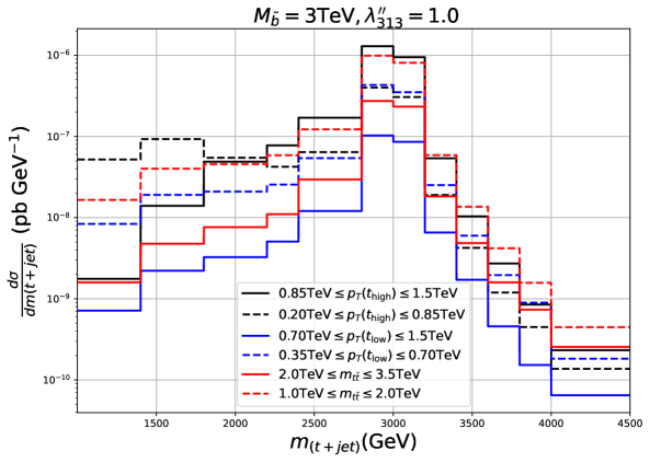
Figure 2: The top + jet invariant mass distributions for the $p~p\rightarrow\tilde{b}^{*}~\bar{t}\rightarrow t~\bar{t}~j$ process as described by the 2nd to 4th diagrams of Fig. 1, for a sbottom mass of $3$ TeV. We have used a Breit–Wigner propagator for the unstable anti-sbottom, with decay width given by eq.(5). The histograms show results after imposing the indicated kinematic cuts. Here $p_{T}(t_{\rm high})$ and $p_{T}(t_{\rm low})$ are the higher and lower transverse momentum of the top or anti-top quark, respectively, and $m_{t\bar{t}}$ is the invariant mass of the $t\bar{t}$ pair.

As mentioned above, in the $t\bar{t}j$ channel, only diagrams corresponding to single sbottom or antisbottom production (shown by the 2nd to 4th diagrams of Fig. 1 and their charge conjugate versions) are considered. Fig. 2 shows the resulting top + jet invariant mass distribution for $M_{\tilde{b}}=3$ TeV for the process $p~p\rightarrow\tilde{b}^{*}~\bar{t}\rightarrow t\bar{t}j$; the charge conjugate process requires a $\bar{d}$ quark in the initial state and therefore has a considerably smaller cross section. We have imposed additional cuts on a quantity characterizing the “hardness” of the process: the higher [$p_{T}(t_{\rm high})$] and lower [$p_{T}(t_{\rm low})$] of the transverse momenta of the $t$ and $\bar{t}$, or the $t\bar{t}$ invariant mass. We see that a prominent peak at $3$ TeV, the mass of the produced $\tilde{b}_{R}^{*}$ squark, remains even if we artificially remove very hard events.

Of course, this peak is not reproduced by the SMEFT. Hence the upper bound on the coupling $\lambda^{\prime\prime}_{313}$ derived in the SMEFT framework is likely to differ significantly from that derived in the RPV model for sbottom mass up to at least $3$ TeV if the contribution of the $t\bar{t}j$ channel remains sizable. For sufficiently large $M_{\tilde{b}}$ the resonance peak will certainly disappear; however, the total sbottom exchange contribution will also become smaller with increasing sbottom mass, hence very large $M_{\tilde{b}}$ will not lead to measurable effects in current LHC data. Alternatively, one could impose an upper cut directly on the invariant mass of the top + jet system, thereby removing the resonance peak. While this would reduce the difference between the SMEFT and RPV results, it would also remove many signal events, and would thus lead to an artificially weakened constraint on the RPV model.

The last three diagrams shown in Fig. 1 contribute to $t\bar{t}jj$ production within the RPV model via the production of a $\tilde{b}_{R}\tilde{b}_{R}^{*}$ pair. Contributions where at least one of them is on–shell again cannot be described by the SMEFT. However, we will see below that for sbottom masses of interest these diagrams contribute little to inclusive $t\bar{t}$ production.

In the following subsections, we will present distributions of the observables that have been measured by CMS or ATLAS; these measurements can be used to constrain the original RPV model or its implementation in the SMEFT using eqs.(7). Recall that our main goal is to check whether the latter gives a faithful representation of the former as far as current LHC data are concerned. The discussion above indicates that this is only true if the contribution from the $t\bar{t}j$ channel to a given distribution is small even in the RPV model and if the RPV model and SMEFT predict similar distributions for the $t\bar{t}$ channel. We will compare the RPV and SMEFT predictions for the relevant distributions assuming $\lambda^{\prime\prime}_{313}=1$, so that the theory remains perturbative up to very high scales. We will also compare the resulting exclusion limits derived in the two frameworks; here we will only require $\lambda^{\prime\prime}_{313}<4.0$ so that the sbottom decay width remains below its mass.

4.3 Transverse momentum of top quarks

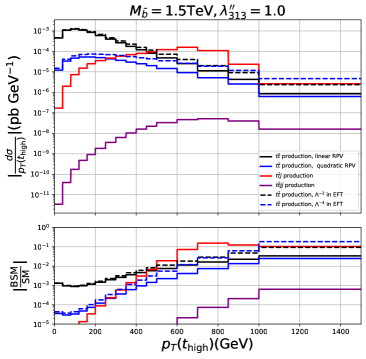
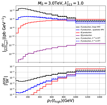
Figure 3: Distributions of $p_{T}(t_{\rm high})$ at parton level predicted by the RPV model (solid) and its SMEFT implementation (dashed). The black histograms show the absolute value of the (negative) interference terms with the QCD diagrams, i.e. the linear new physics contributions to the exclusive $t\bar{t}$ channel. The blue histograms show the square of the $\tilde{b}_{R}$ exchange contribution to the $t\bar{t}$ channel, i.e. the quadratic new physics contributions. The red and violet histograms show the (purely new physics, i.e. quadratic) contributions to the $t\bar{t}j$ and $t\bar{t}jj$ channels, respectively; here only the RPV model contributes to leading order. The left (right) frames are for a sbottom mass of $1.5$ ($3.0$) TeV. The top frames show the absolute distributions, whereas the lower frames show results normalized to the NNLO QCD prediction.

In this subsection, we analyze the transverse momentum distributions of the produced top (anti–)quarks. We begin with Fig. 3, which presents the distributions of the larger of the two $p_{T}$ values, $p_{T}(t_{\rm high})$; only the BSM contributions are shown. The black histograms show the absolute value of the (negative) interference term with the QCD diagrams. The difference between the SMEFT (dashed) and full RPV model (solid) predictions becomes sizable at $p_{T}(t_{\rm high})\simeq M_{\tilde{b}}/3$. Even though this contribution peaks in absolute value at about half the top mass, it falls off less quickly than the pure SM prediction does, i.e. the new contribution becomes more significant at larger $p_{T}(t_{\rm high})$, as shown in the lower frames.

The blue histograms show the squared sbottom exchange contribution to exclusive $t\bar{t}$ production. This contribution, which is ignored in linear SMEFT (or RPV) fits, becomes at least comparable in magnitude to the interference term for $p_{T}(t_{\rm high})\geq 1$ TeV. Moreover, since this contribution contains the square of the sbottom propagator, the difference between the RPV and SMEFT predictions is larger than for the interference term. In fact, the SMEFT predicts that for $M_{\tilde{b}}=1.5$ TeV (left frames) this term dominates over the interference term for $p_{T}(t_{\rm high})\geq 1$ TeV, which does not happen in the full RPV calculation.

Note that the SMEFT prediction always exceeds that of the full RPV model, both in linear and in quadratic order. This can be understood from the observation that a space–like momentum flows through the $\tilde{b}_{R}$ propagator in the first diagram shown in Fig. 1; neglecting the momentum dependence of this propagator, as done in the SMEFT, therefore over–estimates its absolute value.

The red and magenta histograms show contributions from the $t\bar{t}j$ and $t\bar{t}jj$ channels; recall that only the RPV model contributes here at leading order, via the production of one or two on–shell $\tilde{b}_{R}$ (anti–)squarks. We see that for $M_{\tilde{b}}=1.5$ TeV single sbottom production dominates the total RPV contribution for $p_{T}(t_{\rm high})\geq M_{\tilde{b}}/3$. Since the SMEFT treatment predicts too large a contribution at large $p_{T}(t_{\rm high})$, for $M_{\tilde{b}}=1.5$ TeV the production of on–shell sbottom squarks coincidentally improves the agreement between the two predictions in this region. However, for $M_{\tilde{b}}=1.5$ TeV on–shell sbottom production also leads to a pronounced (Jacobian) peak at $p_{T}(t_{\rm high})\simeq M_{\tilde{b}}/2$, where the harder top (anti–)quark predominantly results from the decay of an on–shell $\tilde{b}_{R}$; this is of course not reproduced by the SMEFT prediction. Finally, we see that the $t\bar{t}jj$ contribution, due to $\tilde{b}_{R}\tilde{b}_{R}^{*}$ pair production, remains well below the other contributions even for $M_{\tilde{b}}=1.5$ TeV, and is completely negligible for $M_{\tilde{b}}=3$ TeV.

Table 1: Values of $\frac{\sigma(\text{SMEFT})}{\sigma(\text{RPV})}$ in two bins with moderate and high $p_{T}(t_{\rm high})$ and for two values of the sbottom mass, assuming $\lambda^{\prime\prime}_{313}=1$. The third, fourth and fifth column only refer to the exclusive $t\bar{t}$ channel, showing the ratios of the linear terms, of the quadratic terms, and of the sums of linear and quadratic terms; in this channel $p_{T}(t_{\rm high})=p_{T}(t_{\rm low})$ after correcting to the parton level. The last column shows the ratios for the fully inclusive $t\bar{t}$ cross section, including linear and quadratic contributions and the $t\bar{t}j$ and $t\bar{t}jj$ channels.

$M_{\tilde{b}}$(GeV)	$p_{T}(t_{\text{high}})$ [GeV]	$t\bar{t}$ (linear)	$t\bar{t}$ (quadratic)	$t\bar{t}$ (linear+quadratic)	total
1500	500-600	1.50	2.42	1.10	-0.42
	1000-1500	2.77	7.46	-10.3	0.97
3000	500-600	1.13	1.37	1.10	1.14
	1000-1500	1.50	2.23	1.14	-0.41

The difference between the predictions by the RPV model and its SMEFT implementation are summarized in in Table 1, for different bins of $p_{T}(t_{\rm high})$. As noted above, the difference between the SMEFT and full RPV predictions are larger for smaller sbottom mass, for larger $p_{T}(t_{\rm high})$, and in quadratic (rather than linear) order. Since the interference term is negative while the squared BSM contribution is (of course) positive, the difference between the SMEFT and RPV predictions can be significantly smaller in the sum of linear and quadratic contributions to exclusive $t\bar{t}$ production than it is for either one separately. However, this very same cancellation can also make the full RPV contribution to exclusive $t\bar{t}$ production very small, as in the higher $p_{T}(t_{\rm high})$ bin for the lower sbottom mass; here the SMEFT predictions differs from that of the (more) UV complete theory by an order of magnitude and even gives the wrong sign! As already noted, in this particular case including $t\bar{t}j$ production from (anti)sbottom decay in the RPV happens to give close agreement between the two predictions for inclusive $t\bar{t}$ production; however, doing so leads to very poor agreement in the lower $p_{T}(t_{\rm high})$ bin.

For $M_{\tilde{b}}=3$ TeV and $\lambda^{\prime\prime}_{313}=1$ both the SMEFT and the RPV model predict negative contributions to exclusive $t\bar{t}$ production even in quadratic order; the predictions for the sum of the two contributions happen to agree over a wide range of $p_{T}(t_{\rm high})$. Recall, however, that adding the quadratic contribution in the SMEFT is not well motivated, since it is of the same order in the cut–off parameter $\Lambda$ as contributions from dimension$-8$ operators which are not included. Moreover, the last column shows that this agreement is ruined once the $t\bar{t}j$ channel is included, which turns the total BSM contribution positive at large $p_{T}(t_{\rm high})$ even for this large sbottom mass.

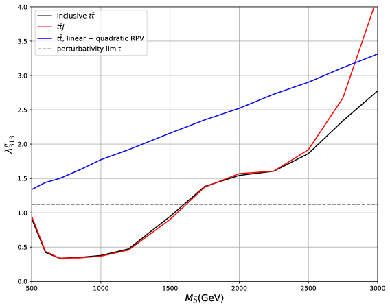
Figure 4: Exclusion limits at $95\%$ confidence level, derived from the parton level distribution of $p_{T}(t_{\rm high})$ measured by CMS CMS:2021vhb . The solid black line depicts the complete RPV bounds from inclusive $t\bar{t}$ production, where all Feynman diagrams shown in Fig. 1 have been taken into account. The blue and red lines depict the bounds derived using only the sbottom contributions to the exclusive $t\bar{t}$ and $t\bar{t}j$ channel, respectively. The upper bound $\lambda^{\prime\prime}_{313}<1.12$ is indicated by the dashed black line.

Fig. 4 presents the $95\%$ c.l. exclusion limits derived by us from the CMS measurement CMS:2021vhb of the parton level $p_{T}(t_{\rm high})$ distribution. We see that for $M_{\tilde{b}}\leq 2.5$ TeV the red curve, which has been derived including $t\bar{t}j$ production only, nearly coincides with the black line, where all diagrams depicted in Fig. 1 have been taken into account. Evidently the complete RPV bound is primarily determined by single sbottom production leading to $t\bar{t}j$ final states. This contribution remains significant even for $M_{\tilde{b}}=3$ TeV. Since it is not included in the SMEFT treatment, bounds derived within the SMEFT framework will not be reliable for any sbottom mass shown.

Considering even larger values of $M_{\tilde{b}}$ would, of course, result in even weaker bounds on the coupling $\lambda^{\prime\prime}_{313}$. Recall that this coupling should be less than $1.12$ for the RPV model to be considered UV–complete, since otherwise a Landau pole will appear well below the scale of Grand Unification; if this bound is imposed, current data are not sensitive to sbottom masses beyond $1.6$ TeV. Moreover, we saw in Table 1 that in the highest $p_{T}(t_{\rm high})$ bin the quadratic SMEFT prediction exceeds that of the RPV model by more than a factor of $2$ even for $M_{\tilde{b}}=3$ TeV; this comparison is independent of the value of $\lambda^{\prime\prime}_{313}$. The two predictions will agree to within, say, $20\%$ only for $M_{\tilde{b}}>5$ TeV. For these very large sbottom masses current data could only exclude values of the coupling $\lambda^{\prime\prime}_{313}$ that badly violate our perturbativity limit of $4$.

We finally note that in the full RPV model the bound on the coupling does not increase monotonically with the sbottom mass. Of course, in the SMEFT implementation only the ratio $\lambda^{\prime\prime}_{313}/M_{\tilde{b}}$ can be constrained, hence the bound on the coupling is necessarily proportional to the mass. In our RPV model the bound on the coupling is strongest for $M_{\tilde{b}}\simeq 750$ GeV. It becomes weaker for smaller sbottom mass since the data actually slightly favor an RPV contribution with $M_{\tilde{b}}\simeq 500$ GeV; however, the difference in $\chi^{2}$ relative to the SM value is not statistically significant.

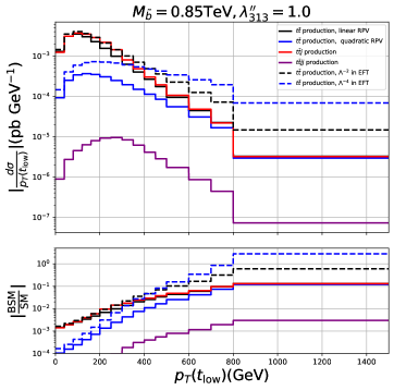
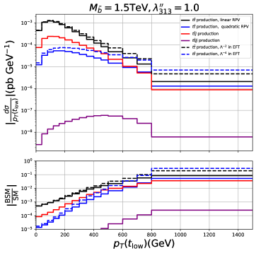
Figure 5: As in Fig.3, but for the $p_{T}(t_{\rm low})$ distribution and reduced values of $M_{\tilde{b}}$.

We now turn to $p_{T}(t_{\rm low})$, the transverse momentum of the softer of $t$ and $\bar{t}$; the corresponding distribution is shown in Fig. 5. Here the contribution from the $t\bar{t}j$ channel, depicted by the red histograms, is not enhanced at $p_{T}(t_{\rm low})\sim\frac{M_{\tilde{b}}}{2}$, since in this channel most of the time the softer top (anti-)quark is not produced from squark decay. As a result this contribution is subdominant already for $M_{\tilde{b}}=1.5$ TeV (right frame), in contrast to the $p_{T}(t_{\rm high})$ distribution shown in the left frame of Fig. 3. This reduces the difference between the RPV and SMEFT predictions for the $p_{T}(t_{\rm low})$ distribution.

For $M_{\tilde{b}}=0.85$ TeV (left frame of Fig. 5) the $t\bar{t}j$ contribution is sizable in all bins, indicating that the SMEFT description will not work. Recall that the interference contribution depicted by the black histogram is negative; clearly in the given example there’s a strong cancellation between the new contributions to the exclusive $t\bar{t}$ channel and the new $t\bar{t}j$ channel, at least as far as the $p_{T}(t_{\rm low})$ distribution is concerned. Not surprisingly, for this smaller value of $M_{\tilde{b}}$ the discrepancy between the SMEFT and full RPV predictions for the exclusive $t\bar{t}$ channel becomes larger. For example, the SMEFT predicts that the (positive) quadratic term exceeds the (negative) linear one for $p_{T}(t_{\rm low})>500$ GeV; in the full RPV this does not happen at all, at least not in the range of transverse momenta shown. Note that in the exclusive $t\bar{t}$ channel at leading order the $p_{T}(t_{\rm high})$ and $p_{T}(t_{\rm low})$ distributions are identical due to transverse momentum conservation, i.e., $p_{T}(t_{\rm high})\equiv p_{T}(t_{\rm low})\equiv p_{T}(t)\equiv p_{T}(\bar{t})$.

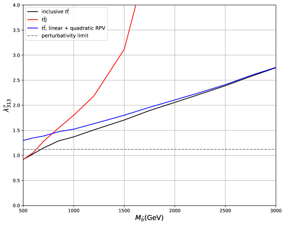
Figure 6: As in Fig. 4, but for exclusion limits derived from the $p_{T}(t_{\rm low})$ distribution.

Since single $\tilde{b}_{R}$ production leading to the $t\bar{t}j$ channel is much less important in the $p_{T}(t_{\rm low})$ distribution than in the $p_{T}(t_{\rm high})$ distribution, we expect the former to lead to weaker bounds on the model parameters. This is confirmed by Fig. 6, which presents the exclusion limits at $95\%$ CL obtained from the CMS measurement CMS:2021vhb of this (parton–level) distribution. The black line, which shows the complete RPV bound including all channels, now only coincides with the red line derived from the $t\bar{t}j$ channel alone only for $M_{\tilde{b}}\simeq 500$ GeV. For $M_{\tilde{b}}\geq 2$ TeV the black line nearly coincides with the blue one, which has been obtained from the exclusive $t\bar{t}$ channel alone, showing that the contribution from the $t\bar{t}j$ channel becomes negligible here. Recall, however, that the SMEFT does not reproduce the tail of the $p_{T}$ distribution of the top (anti-)quark very well even for $M_{\tilde{b}}=3$ TeV, see Table 1. Moreover, current data for $p_{T}(t_{\rm low})$ lose sensitivity to sbottom exchange or production once $M_{\tilde{b}}>680$ GeV if we demand that the theory remains perturbative to very high energy scales.

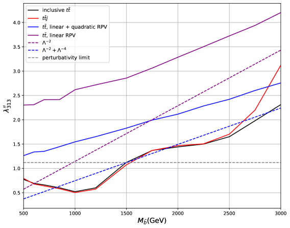
Figure 7: Exclusion limits derived from the $p_{T}(t_{h})$ distribution, where $t_{h}$ denotes the hadronically decaying top (anti-)quark. The solid purple line depicts the bound derived from the linear RPV contribution to the exclusive $t\bar{t}$ channel only; the meaning of the other solid lines is as in Fig. 4. The dashed purple and blue lines show the bounds derived from the SMEFT in linear and linear + quadratic order, respectively; they correspond to $\lambda^{\prime\prime}_{313}/M_{\tilde{b}}=1.14$ and $0.75$, respectively.

CMS also presents a measurement CMS:2021vhb of the parton–level $p_{T}(t_{h})$ distribution, where $t_{h}$ denotes the hadronically decaying top (anti-)quark, the other one decaying semi–leptonically. Following Ref. Catani:2019hip we compute the $p_{T}(t_{h})$ distribution by averaging the $p_{T}$ distributions of the top quark and antiquark; of course, in the exclusive $t\bar{t}$ channel we have $p_{T}(t_{h})=p_{T}(t)=p_{T}(\bar{t})$.

The resulting exclusion limits are shown in Fig. 7. The complete RPV bound (black solid line) is comparable to that obtained from the $p_{T}(t_{\rm high})$ distribution (slightly weaker at small $M_{\tilde{b}}$ and slightly stronger at larger $M_{\tilde{b}}$), but stronger than that derived from the $p_{T}(t_{\rm low})$ distribution. It intersects the upper bound (4) on $\lambda^{\prime\prime}_{313}$ at $M_{\tilde{b}}\sim 1.5$ TeV.

We also show the limit obtained by considering only the the exclusive $t\bar{t}$ channel. The solid (dashed) purple and blue lines refer to the bounds derived from linear RPV (SMEFT) and linear+quadratic RPV (SMEFT) contributions, respectively. We first note that including the square of the new contribution leads to much stronger constraints. Even on the solid blue curve $\lambda^{\prime\prime}_{313}/M_{\tilde{b}}$ is considerably larger than in Figs. 3 and 5. This is significant since the ratio of the square of the new contribution to the interference term scales like $\left(\lambda^{\prime\prime}_{313}/M_{\tilde{b}}\right)^{2}$, hence along this line the quadratic terms are relatively much more important than in our earlier example with $\lambda^{\prime\prime}_{313}=1$. On or near the bound the quadratic terms thus always dominate at large $p_{T}(t_{h})$.

By comparing lines of the same color, it is clear that the SMEFT considerably overestimates the bounds, compared to those derived within the UV complete RPV model. This agrees with our earlier observation in Figs. 3 and 5 and Table 1 that the SMEFT significantly overestimates the squark exchange contribution even at $M_{\tilde{b}}=3$ TeV, especially in the bins with high $p_{T}$ where this contribution is most significant. Evidently the quadratic SMEFT constraint very roughly reproduces the complete RPV result. However, this is largely accidental, and also misses that in the RPV model the bound on the coupling is not strictly proportional to $M_{\tilde{b}}$. In particular, the bound gets weaker at the smallest sbottom masses shown because the data again mildly prefer a non–vanishing RPV contribution. We also remind the reader that in the SMEFT framework including the square of $d=6$ operators but ignoring all $d=8$ operators is not really consistent.

4.4 Invariant mass of the top pair

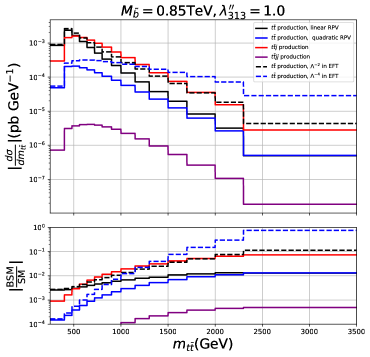
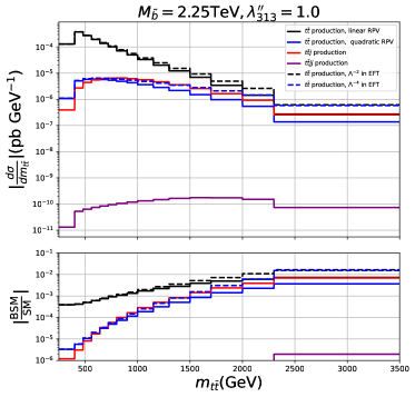
Figure 8: As in Fig. 3, but for the $m_{t\bar{t}}$ distribution.

We next turn to the distribution of the invariant mass of the $t\bar{t}$ pair. Fig. 8 shows various BSM contributions to this distributions derived from the RPV model (solid) and its SMEFT implementation (dashed). As before, the lower frames show that the BSM signal becomes more significant in the higher bins where the SM contribution is strongly suppressed. The contribution from the $t\bar{t}jj$ channel is again negligible in all bins. Moreover, for $M_{\tilde{b}}=0.85$ TeV the $t\bar{t}j$ channel dominates for all $m_{t\bar{t}}>700$ GeV, while for $M_{\tilde{b}}=2.25$ TeV this is true in the last two bins. Moreover, the SMEFT again predicts too large contributions to the exclusive $t\bar{t}$ channel. As before, the discrepancy becomes worse for smaller $M_{\tilde{b}}$ and in the higher bins, becoming significant for $m_{t\bar{t}}\gtrsim M_{\tilde{b}}$; it is also worse in the quadratic terms than in the linear one.

Table 2: Values of $\frac{\sigma(\text{SMEFT})}{\sigma(\text{RPV})}$ in two bins with moderate and high $m_{t\bar{t}}$ and for two values of the sbottom mass, assuming $\lambda^{\prime\prime}_{313}=1$. The third, fourth and fifth column only refer to the exclusive $t\bar{t}$ channel, showing the ratios of the linear terms, of the quadratic terms, and of the sums of linear and quadratic terms. The last column shows the ratios for the fully inclusive $t\bar{t}$ cross section, including linear and quadratic contributions and the $t\bar{t}j$ and $t\bar{t}jj$ channels.

$M_{\tilde{b}}$(GeV)	$m_{t\bar{t}}$ [GeV]	$t\bar{t}$ (linear)	$t\bar{t}$ (quadratic)	$t\bar{t}$ (linear+quadratic)	total
850	720-800	1.50	2.26	1.23	-0.74
	2300-3500	8.88	57.2	2050.04	8.62
2250	720-800	1.08	1.16	1.08	1.15
	2300-3500	2.26	4.24	0.27	-0.3

Some results for the ratio $\sigma(\text{SMEFT})/\sigma(\text{RPV})$ are collected in Table 2. The overall trends are quite similar to those in Table 1. In particular, satisfactory agreement is found only for $m^{2}_{t\bar{t}}\ll M^{2}_{\tilde{b}}$, as in the penultimate row of Table 2; otherwise even the sign of the BSM contribution to inclusive $t\bar{t}$ production might be predicted incorrectly by the SMEFT.

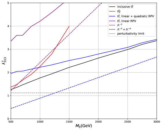
Figure 9: As in Fig. 4, but for exclusion limits derived from the $m_{t\bar{t}}$ distribution measured by CMS. The dashed purple and blue lines correspond to $\lambda^{\prime\prime}_{313}/M_{\tilde{b}}=2.43$ and $0.89$ from including only linear and linear + quadratic SMEFT terms in the computation, respectively.

Fig. 9 presents the exclusion limits at $95\%$ CL which we derive from the CMS measurement CMS:2021vhb of the parton–level $m_{t\bar{t}}$ distribution, again using a $\chi^{2}$ fit. The complete RPV bound depicted by the black line is weaker than those derived from the $p_{T}(t_{\rm high})$ or $p_{T}(t_{h})$ distributions, where on–shell single $\tilde{b}_{R}$ production led to a pronounced (Jacobian) peak in the distribution. In the case at hand the BSM contribution is more widely distributed. Moreover, large values of $m_{t\bar{t}}$ do not necessarily require very large momentum flow through a $t-$ or $u-$channel propagator, while large top transverse momenta do; the $\tilde{b}$ exchange contributions to the exclusive $t\bar{t}$ channel are therefore less enhanced at large $m_{t\bar{t}}$ than at large top $p_{T}$. As a result of these effects, the bound on $\lambda^{\prime\prime}_{313}$ is weaker than the limit (4) even for the smallest $M_{\tilde{b}}$ considered. By comparing the black, red, and blue solid lines we see that the $t\bar{t}j$ channel dominates the determination of the bound for light sbottom, while the exclusive $t\bar{t}$ channel dominates for heavy sbottom.

The SMEFT implementation of our model in terms of $4-$quark operators yields the the upper bounds $\lambda^{\prime\prime}_{313}/M_{\tilde{b}}<2.43$ and $0.89$ when only the $\Lambda^{-2}$ term and both $\Lambda^{-2}+\Lambda^{-4}$ terms are included in the simulation, respectively, as shown by the dashed lines. When only the exclusive $t\bar{t}$ channel is considered these bounds are much stronger than the corresponding limits derived in the RPV model. The SMEFT bound derived in linear order is coincidentally close to the full RPV constraint for the smallest sbottom mass shown, but has too steep a slope; while the quadratic SMEFT limit is even stronger than the RPV bound after inclusion of the $t\bar{t}j$ channel. The two bounds differ by more than $25\%$ even at $M_{\tilde{b}}=3$ TeV; here the true bound on the coupling lies at $3.3$, which would lead to a Landau pole at an energy scale of less than $10$ TeV Allanach:1999mh .

4.5 Transverse momentum of the top pair

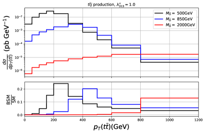
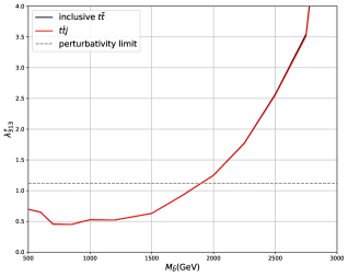
Figure 10: Left: parton–level $p_{T}(t\bar{t})$ distribution predicted by the RPV model. Right: $95\%$ CL exclusion limits derived on the RPV model using the CMS measurement of the $p_{T}(t\bar{t})$ distributions.

The production of one or two real sbottom (anti-)squarks gives a transverse momentum to the $t\bar{t}$ pair in the final state already in leading order. The resulting distribution is shown in the left panel of Fig. 10, where we have neglected the (very small) contribution from the $t\bar{t}jj$ channel, i.e. only included single $\tilde{b}_{R}$ production. Due to the conservation of transverse momentum, $p_{T}({t\bar{t}})$ is equal to the transverse momentum of the light quark jet originating from sbottom decay; this distribution therefore also peaks around $M_{\tilde{b}}/2$, just like the contribution from the $t\bar{t}j$ channel to the $p_{T}(t_{\rm high})$ distribution does. We also note that increasing the sbottom mass reduces the value of the cross section at the peak, but increases the cross section in the last bin. This effect cannot be reproduced by the SMEFT implementation of the RPV model, where the transverse momentum of the $t\bar{t}$ system remains zero in leading order.

The right panel of Fig. 10 shows the $95\%$ CL exclusion limit that we derived within the RPV model from the CMS measurement CMS:2021vhb of the parton–level $p_{T}(t\bar{t})$ distribution. As already noted, in leading order basically only the $t\bar{t}j$ channel contributes. For $0.55$ TeV $<M_{\tilde{b}}<1.24$ TeV the resulting bound on the coupling is slightly weaker than that we derived from the $p_{T}(t_{\rm high})$ distribution, see Fig. 4. However, it increases less fast for larger sbottom mass, remaining stronger than the high–scale perturbativity constraint (4) for $M_{\tilde{b}}<1.9$ TeV; it thus offers the best sensitivity so far for $1.24$ TeV $<M_{\tilde{b}}<2.1$ TeV. A slightly negative $\Delta\chi^{2}$ occurs again for $\lambda^{\prime\prime}_{313}\leq 0.5$ and $M_{\tilde{b}}\simeq 500$ GeV.

4.6 Charge asymmetry of the top pair

Our final observable is the top pair charge asymmetry. Its integrated value has been measured by ATLAS ATLAS:2022waa to be $0.0068\pm 0.0015$, which differs from zero by $4.7$ standard deviations. Following the notation of Ref. Czakon:2017lgo , the charge asymmetry ($A_{C}^{t\bar{t}}$) is defined as,

$$A_{C}^{t\bar{t}}=\frac{\sigma_{\text{bin}}(\Delta|y_{t\bar{t}}|>0)-\sigma_{\text{bin}}(\Delta|y_{t\bar{t}}|<0)}{\sigma_{\text{bin}}(\Delta|y_{t\bar{t}}|>0)+\sigma_{\text{bin}}(\Delta|y_{t\bar{t}}|<0)}$$ (9)

where $\Delta|y_{t\bar{t}}|=|y_{t}|-|y_{\bar{t}}|$ is the difference between the absolute rapidities of top quark and top anti-quark. In this subsection we analyze the differential measurements of this quantity as function of $m_{t\bar{t}}$ and of $p_{T}(t\bar{t})$.

In order to compute the charge asymmetry, we include the SM and BSM contributions to both the numerator and the denominator in eq.(9), where the BSM contribution is again computed either from from the RPV model or from its SMEFT implementation. The BSM contributions are obtained from our LO simulations, while the SM contributions are determined to NNLO QCD with the help of the HighTEA public tool Czakon:2023hls . We use this tool to generate the cross section (the denominator) with the same PDF set, renormalization, and factorization scales as those used in the ATLAS report ATLAS:2022waa . Since the parton–level charge asymmetry from NNLO SM is provided in this report, the SM contribution to the numerator is computed as the product of the quoted charge asymmetry and the NNLO cross section computed by us using HighTEA.

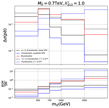
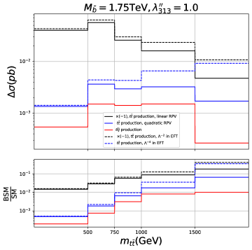
Figure 11: The BSM contribution $\Delta\sigma$ to the numerator of eq.(9) as a function of $m_{t\bar{t}}$. The notation is as in Fig. 3, except that we don’t show the contribution from the $t\bar{t}jj$ final state since it vanishes in leading order.

Fig. 11 shows the BSM contribution to the numerator $\Delta\sigma$ of eq.(9). These contributions are non–zero since the four–quark operators given in eqs.(6) only include right–handed quarks, i.e. they contain the chiral projector $P_{R}$. The resulting $\gamma_{5}$ terms give rise to a forward–backward asymmetry in the partonic center–of–mass frame, which in turn leads to a non–vanishing charge asymmetry even in leading order. In contrast, in QCD a charge asymmetry only appears at NLO, and only for top pair production from quark annihilation; gluon fusion processes do not contribute to $\Delta\sigma$. To linear order both the RPV model and its SMEFT implementation predict $\Delta\sigma$ to be negative; Fig. 11 shows their absolute value. We see that the contribution from the $t\bar{t}j$ channel, which only exists in the RPV model, is quite large for $M_{\tilde{b}}=0.7$ TeV (left frames), while it is negligible for $M_{\tilde{b}}=1.75$ TeV. In the exclusive $t\bar{t}$ channel the SMEFT implementation again over–predicts the BSM contribution, particularly in the high bins.

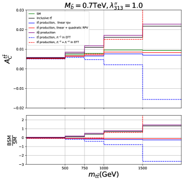
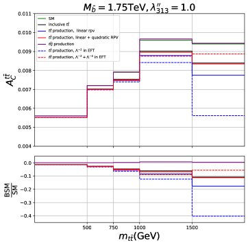
Figure 12: Charge asymmetry as function of $m_{t\bar{t}}$. The green histogram shows the SM prediction for $A_{C}^{t\bar{t}}$. The other histograms depict predictions for $A_{C}^{t\bar{t}}$ including BSM contributions in addition to that from the SM, with $\lambda^{\prime\prime}_{313}=1$. As before, solid and dashed histograms show predictions by the RPV model and its SMEFT implementation, with blue and red histograms showing predictions for the exclusive $t\bar{t}$ channel to linear and quadratic order, respectively. The purple histogram depicts the contribution from the $t\bar{t}j$ channel, and the black histogram shows the complete RPV prediction. The lower panels show the difference between BSM and predictions normalized to the SM.

Fig. 12 shows predictions for the charge asymmetry as function of $m_{t\bar{t}}$. The SM prediction is shown by the green histogram; its contribution has been included in all other histograms as well, which assume $\lambda^{\prime\prime}_{313}=1$. Including only linear (i.e. interference) BSM contributions (blue) reduces the charge asymmetry, but the RPV model predicts it to remain positive even for $M_{\tilde{b}}=0.7$ TeV (left frames). In contrast, the SMEFT implementation to linear order predicts a negative charge asymmetry for such a small sbottom mass and large $t\bar{t}$ invariant mass. Including the quadratic terms (red) brings the RPV prediction for the exclusive $t\bar{t}$ channel quite close to the SM, and leads to a positive charge asymmetry even in the SMEFT implementation; the latter becomes quite large (off the scale shown) for $M_{\tilde{b}}=0.7$ TeV.

The $t\bar{t}j$ channel (violet), which receives LO contributions only in the RPV model with on–shell $\tilde{b}_{R}$ production, is always positive. Comparison with the black histogram, which shows the complete prediction in the RPV model, shows that on–shell $\tilde{b}_{R}$ production dominates the charge asymmetry for $M_{\tilde{b}}=0.7$ TeV. This contribution is suppressed for $M_{\tilde{b}}=1.75$ TeV (right frames). For this combination of $\tilde{b}_{R}$ mass and RPV coupling the total RPV contribution therefore reduces the charge asymmetry. This is true also in the SMEFT implementation, which however predicts the difference from the SM prediction to be too small by nearly a factor of two in the last bin even for $M_{\tilde{b}}=1.75$ TeV.

Table 3: Values of $\frac{F(\text{SM+EFT})-F(\text{SM})}{F(\text{SM}+\text{RPV})-F(\text{SM})}$ in the exclusive $t\bar{t}$ channel for two bins of $m_{t\bar{t}}$, two values of the sbottom mass, and two values of the RPV coupling $\lambda^{\prime\prime}_{313}$. In the third to sixth columns, $F$ is the charge asymmetry, while in the last two columns $F$ is $\Delta\sigma$. The upper index $l$ stands for linear RPV or SMEFT contributions, while $l+q$ includes the quadratic contribution. The values of the coupling are shown in parentheses. For example, $A^{l+q}_{C}(3)$ is the charge asymmetry derived from linear + quadratic RPV or SMEFT with $\lambda^{\prime\prime}_{313}=3$.

$M_{\tilde{b}}$	$m_{t\bar{t}}$	$A^{l}_{C}(1)$	$A^{l+q}_{C}(1)$	$A^{l}_{C}(3)$	$A^{l+q}_{C}(3)$	$\Delta\sigma^{l}$	$\Delta\sigma^{l+q}(1)$
$0.7$ TeV	$500-750$ GeV	1.69	1.31	1.71	3.05	1.68	1.31
	$>1500$ GeV	10.2	-72.8	20.3	7.30	9.56	-92.9
$1.75$ TeV	$500-750$ GeV	1.12	1.11	1.12	1.00	1.12	1.11
	$>1500$ GeV	2.29	0.5	2.38	4.88	2.27	0.5

A more quantitative comparison between the prediction of the full RPV model and its SMEFT implementation is shown in Table 3, which gives some values of $\frac{A_{C}^{t\bar{t}}(\text{SM+EFT})-A_{C}^{t\bar{t}}(\text{SM})}{A_{C}^{t\bar{t}}(\text{SM}+\text{RPV})-A_{C}^{t\bar{t}}(\text{SM})}$ in the third to sixth columns and the corresponding values of $\Delta\sigma(\text{SMEFT})/\Delta\sigma(\text{RPV})$ in the last two columns. For $M_{\tilde{b}}=0.7$ TeV the discrepancy is large even in the lower invariant mass bin; for $\lambda^{\prime\prime}_{313}=1$ adding the quadratic contributions, which is perfectly reasonable in the RPV model but less so in its SMEFT implementation, reduces the discrepancy due to cancellations between the linear and quadratic contributions. In the higher invariant mass bin the discrepancy becomes very large. Since in this bin the BSM contribution is sizable in both the numerator and denominator of the definition (9) of the charge asymmetry the ratio of the RPV and SMEFT predictions for this asymmetry depends on the coupling even to linear order, whereas the ratio of the predicted $\Delta\sigma$ values (shown in the seventh column) does not.

Increasing the sbottom mass to $1.75$ TeV leads to fairly good agreement between the predictions in the lower invariant mass bin; however, in the bin with large invariant mass, where the deviation from the SM prediction is much more prominent as shown in the lower frames of Fig. 12, the two predictions still differ by a factor of $2$ or more.

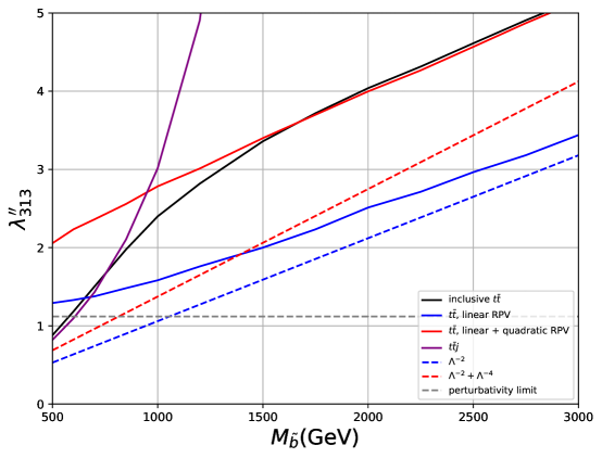
Figure 13: Similar to Fig. 4, but for exclusion limits derived from the ATLAS measurement ATLAS:2022waa of the charge asymmetry as a function of $m_{t\bar{t}}$. The SMEFT implementation of our RPV model leads to the upper bounds $\lambda^{\prime\prime}_{313}/M_{\tilde{b}}<1.06$ ($1.37$) in linear (linear plus quadratic) order, respectively, as shown by the dashed lines.

Fig. 13 presents $95\%$ CL exclusion limits obtained from the ATLAS measurement ATLAS:2022waa of the parton–level charge asymmetry as a function of $m_{t\bar{t}}$. The complete RPV model leads to a rapidly weakening bound as the sbottom mass in increased. The $t\bar{t}j$ channel dominates the determination of the bound for $M_{\tilde{b}}\leq 750$ GeV, while the exclusive $t\bar{t}$ channel dominates for heavy sbottom. Overall the bound is quite weak, excluding couplings below the bound (4) from demanding perturbative unitarity up to very high energy scales only for $M_{\tilde{b}}<570$ GeV. Moreover, the SMEFT implementation again leads to much too strong constraints for the entire range of sbottom mass shown. In contrast to the bounds derived from the $p_{T}$ spectrum of top (anti–)quarks or from the $t\bar{t}$ invariant mass spectrum, including quadratic SMEFT contributions weakens the constraint, since they don’t suffice to flip the sign of the linear (interference) contribution even in the highest bins.

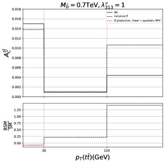
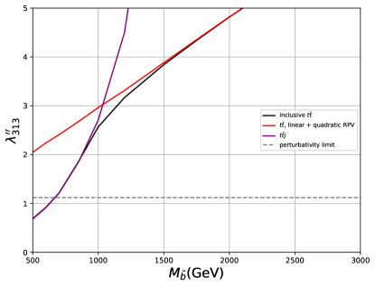
Figure 14: Left: the charge asymmetry defined in eq.(9) as function of $p_{T}(t\bar{t})$, as predicted in the SM (solid) and in the RPV theory (dashed). The dashed red histogram is for the exclusive $t\bar{t}$ channel, which to leading order only contributes in the first bin; in this bin it overlaps with the dashed black histogram which shows the RPV prediction for inclusive $t\bar{t}$ production. Right: the $95\%$ CL exclusion limit derived in the framework of the RPV model from the ATLAS measurement ATLAS:2022waa of the the charge asymmetry as a function of $p_{T}{(t\bar{t})}$.

The left panel of Fig. 14 presents the predicted charge asymmetry as a function of $p_{T}(t\bar{t})$ for $M_{\tilde{b}}=0.7$ TeV and $\lambda^{\prime\prime}_{313}=1$. Sbottom exchange to the exclusive $t\bar{t}$ channel contributes to leading order only at $p_{T}(t\bar{t})=0$, as shown by the red dashed histogram. The deviations of $A_{C}^{t\bar{t}}$ in the second and third bins are thus entirely due to the $t\bar{t}j$ channel. Since this contribution is peaked at $p_{T}(t\bar{t})\simeq M_{\tilde{b}}/2$ it is most prominent in the highest bin.

Recall that the QCD prediction is at NNLO, and therefore extends to non–vanishing $p_{T}(t\bar{t})$. Since gluons emit more initial state radiation than quarks do, the gluon fusion channel, which does not contribute to the numerator of the charge asymmetry, is less important in the lowest bin, but completely dominates the second bin; this explains the steep decline of the SM prediction between these two bins. At very large values of $p_{T}(t\bar{t})$ the contribution from $q\bar{q}$ annihilation becomes somewhat more important again since the valence quark distributions are harder than the gluon distribution in the proton; as a result the SM prediction increases again in the third, and highest, bin.

The right panel of Fig. 14 depicts $95\%$ CL exclusion limits obtained from the ATLAS measurement ATLAS:2022waa of the parton–level charge asymmetry as a function of $p_{T}(t\bar{t})$. The complete RPV bound (black) is essentially determined by the $t\bar{t}j$ channel (purple) for $M_{\tilde{b}}<1$ TeV. However, for $M_{\tilde{b}}\leq 0.9$ TeV the bound on the RPV coupling is only slightly stronger than that derived from the distribution of the charge asymmetry as function of $m_{t\bar{t}}$, see Fig. 13, and even weaker for larger sbottom mass. The bound falls below the perturbative unitarity limit (4) only for $M_{\tilde{b}}<670$ GeV.

4.7 Summary of exclusion limits in the RPV model and its SMEFT implementation

Figure 15: Summary of $95\%$ CL exclusion limits on the RPV coupling as function of the sbottom mass. The solid curves have been derived from CMS measurements CMS:2021vhb of the inclusive $t\bar{t}$ production cross section differential in some transverse momentum or in the $t\bar{t}$ invariant mass, while the dashed green and purple curves have been derived from ATLAS measurements ATLAS:2022waa of the charge asymmetry in inclusive $t\bar{t}$ production. The dashed gray line shows the bound (4) from demanding perturbative unitarity up to very high energy scales; for $\lambda^{\prime\prime}_{313}>3$ perturbation theory becomes questionable even at the scales probed at the LHC.

Fig. 15 collects the limits on the RPV coupling derived in the full RPV model as discussed in the previous subsections. We see that the strongest upper bound on the coupling comes from either the $p_{T}(t_{\rm high})$ distribution (solid black), the $p_{T}(t_{h})$ distribution (solid red) or the $p_{T}(t\bar{t})$ distribution (solid purple), depending on the value of $M_{\tilde{b}}$. Since these three bounds have been derived from the same data set CMS:2021vhb their statistical combination is not straightforward; lacking such a combination one can simply take the strongest of these three limits as final bound derived from the CMS data. The resulting upper bound on $\lambda^{\prime\prime}_{313}$ is stronger than the constraint (4) from high–scale unitarity for $M_{\tilde{b}}<1.9$ TeV.

In Fig. 15 we extend the constraints to $M_{\tilde{b}}=3$ TeV and allow values of the coupling $\lambda^{\prime\prime}_{313}\leq 4$. It should be noted that the Breit–Wigner propagator, with constant (energy independent) width, is used for the unstable sbottom in the $t\bar{t}j$ and $t\bar{t}jj$ channels. This becomes a rather poor approximation for $\lambda^{\prime\prime}_{313}\gtrsim 3$, as mentioned in Sec. 2. One reason is that the width originates from the imaginary part of the $\tilde{b}_{R}$ two–point function, which depends on the square of the four–momentum $q^{2}$ flowing through it; if the width is a sizable fraction of $M_{\tilde{b}}$ it will remain important over an extended range of $q^{2}$, where the imaginary part varies considerably. For $q^{2}\sim M^{2}_{\tilde{b}}$ these diagrams are therefore specially sensitive to loop corrections.

In the $\tilde{b}_{R}$ exchange contribution to exclusive $t\bar{t}$ production, described by the first diagram in Fig. 1, the exchanged momentum is space–like, hence the corresponding two–point function has no imaginary part. However, the real part of the two–point function will modify the $t-$channel $\tilde{b}_{R}$ propagator at one–loop order. Recall also that the $t\bar{t}j$ channel affects the bound on $\lambda^{\prime\prime}_{313}$ even for $M_{\tilde{b}}\simeq 3$ TeV. Therefore the bounds shown in Fig. 15 may not be very reliable for $\lambda^{\prime\prime}_{313}>3$. Since our LO calculation almost certainly cannot be trusted for $\lambda^{\prime\prime}_{313}>4$ we do not extend our bounds to such large couplings.

Recall that the three observables giving the best bounds on our RPV coupling are not described well by the SMEFT implementation of the RPV model. In leading order $p_{T}(t\bar{t})$ gets contributions only from the $t\bar{t}j$ and $t\bar{t}jj$ channels, which do not exist in the SMEFT implementation. The $t\bar{t}j$ channel also makes significant contributions to $p_{T}(t_{\rm high})$ and $p_{T}(t_{h})$ even at $M_{\tilde{b}}=3$ TeV. The discrepancy between the RPV model and its SMEFT implementation was smaller in the $p_{T}(t_{\rm low})$ distribution, which however yields a much weaker constraint on $\lambda^{\prime\prime}_{313}$.

Table 4: $95\%$ CL bounds on the Wilson coefficients of the two $d=6$ SMEFT operators generated at tree–level from the RPV model, in units of $\text{TeV}^{-2}$. The second and third column are taken from ref.Ethier:2021bye ; “Individual” means that only a single Wilson coefficient is allowed to be nonzero, whereas “Marginalized” refers to the results of a fit where up to $50$ coefficients are allowed to float. The next three columns show results derived by us, as described earlier in this section. The last column shows individual results from the ATLAS collaboration ATLAS:2022waa , using their measurement of the charge asymmetry.

Operator	Individual	Marginalized	$p_{T}(t_{h})$	$m_{t\bar{t}}$	$A_{C}^{t\bar{t}}(m_{t\bar{t}})$	$A_{C}^{t\bar{t}}(m_{t\bar{t}})$, ATLAS
$\Lambda^{-2}$
$\mathcal{O}_{td}^{(1)}$	[-9.504,-0.086]	[-27.673,11.356]				[-1.94,1.00]
$\mathcal{O}_{td}^{(8)}$	[-1.458,1.365]	[-5.494,25.358]	-1.300	-5.905	-1.124	[-0.45,2.13]
$\Lambda^{-2}+\Lambda^{-4}$
$\mathcal{O}_{td}^{(1)}$	[-0.449,0.371]	[-0.474,0.347]	0.188	0.264	0.626	[-0.60,0.84]
$\mathcal{O}_{td}^{(8)}$	[-1.308,0.638]	[-1.329,0.643]	-0.563	-0.792	-1.877	[-1.62,1.21]

For completeness we nevertheless collect in Table 4 the bounds on the Wilson coefficients of the two $d=6$ SMEFT operators that are generated at tree–level by our RPV model. The second and third columns show fit results from ref.Ethier:2021bye , which predates the publication of the CMS and ATLAS data we used for our analysis. The next three columns show the constraints we derived from the measured $p_{T}(t_{h}),\ m_{t\bar{t}}$ and $A_{C}^{t\bar{t}}(m_{t\bar{t}})$ distributions, respectively, and the last column shows the constraints derived by ATLAS ATLAS:2022waa from the latter distribution. Note that in our analysis we always assume $C^{1}_{td}=-C^{8}_{td}/3>0$, see eqs.(7), whereas in refs.Ethier:2021bye and ATLAS:2022waa these two coefficients are assumed to be independent and are allowed to have either sign. Moreover, we only include $d$ (anti–)quarks in the initial state, whereas refs.Ethier:2021bye and ATLAS:2022waa assume equal couplings for $d$ and $s$ quarks; however, since there are no strange valence quarks in the proton the additional contribution from $s\bar{s}$ initial states is quite small.

A final difference is that we only consider LO QCD matrix elements when computing the interference with SMEFT operators (or with the full matrix element predicted by the RPV model), whereas refs.Ethier:2021bye and ATLAS:2022waa also include electroweak contributions to the SM amplitudes. This explains why these references obtain a bound on $C^{1}_{td}$ already a linear order; recall that ${\cal O}^{(1)}_{td}$ does not interfere with the LO QCD contribution to $d\bar{d}\rightarrow t\bar{t}$, due to the different color structure. However, these bounds are not very strong.

We see that the bound on $C^{8}_{td}$ that we derive to linear order from either the $p_{T}(t_{h})$ or the $A_{C}^{t\bar{t}}(m_{t\bar{t}})$ distributions is comparable to the corresponding individual constraint from ref.Ethier:2021bye , remembering that we only allow negative values for this coefficient. This indicates that including these observables into a global SMEFT fit might have some impact even on the individual fit; the impact would be much greater if these measurements break some degeneracy, which must be responsible for the greatly weakened bounds in the marginalized fit. We also note that the ATLAS constraint on this coefficient is considerably stronger on the negative side than what we find. This is probably because they define their allowed interval relative to the best–fit value, which is positive in this case. We define our $\Delta\chi^{2}$ relative to the SM prediction (which is also the best–fit value after imposing our constraint $C^{8}_{td}\leq 0$).

We also see that including the $\Lambda^{-4}$ contributions, i.e. performing a quadratic fit, greatly changes the constraints. In this case the constraint on $C^{8}_{td}$ we derive from the $p_{T}(t_{h})$ or $m_{t\bar{t}}$ distribution is considerably stronger even than the individual fits in the literature; since $\left|C^{1}_{td}\right|^{2}=\left|C^{8}_{td}\right|^{2}/9$ the fact that we include two operators probably only plays a comparatively minor role here. The inclusion of the differential $t\bar{t}$ distributions measured by the CMS collaboration should therefore have a sizable impact on the quadratic fit even if the methodology of ref.Ethier:2021bye is adopted.

However, the large difference between the results of the linear and quadratic fits also shows that these bounds are not reliable even within the framework of the SMEFT. As we emphasized previously, to ${\cal O}(\Lambda^{-4})$ one should also include the interference of $d=8$ SMEFT operators with the SM contribution, at least in the marginalized fit. Some of these contributions can surely be negative, whereas the square of $d=6$ operators can obviously only increase cross sections. More fundamentally, finding large differences in ${\cal O}(\Lambda^{-2})$ and ${\cal O}(\Lambda^{-4})$ fits shows that the expansion in inverse powers of $\Lambda$ does not converge when applied to current LHC data, casting doubt on the principle by which the SMEFT is constructed.

5 Conclusions

In this paper we tested how well a simplified supersymmetric model with $R-$parity violation can be described by $d=6$ $4-$quark operators contained in the SMEFT. Specifically, we considered contributions from $\tilde{b}_{R}$ exchange to inclusive top pair production. This analysis is facilitated by the fact that CMS CMS:2021vhb and ATLAS ATLAS:2022waa show various measured distributions at the parton level, which we can directly compare to parton–level simulations. We assume that the $\tilde{b}_{R}$ is considerably lighter than all other supersymmetric particles, so that their production can be ignored; and that the only non–zero new coupling is $\lambda_{313}^{\prime\prime}$. These assumptions are not particularly “natural” from the supersymmetric model building point of view, but they are “SMEFT friendly”, since the latter cannot be expected to correctly model the production of (for example) on–shell gluinos. We saw in Sec. 3 that direct searches do not seem to constrain this scenario strongly. We therefore consider sbottom masses from $0.5$ TeV upwards.

The coefficients of the relevant $4-$ quark operators ${\cal O}^{(1)}_{td}$ and ${\cal O}^{(8)}_{td}$ can easily be obtained by integrating out $\tilde{b}_{R}$ at tree level, see eqs.(7). Clearly this SMEFT implementation of the RPV model can only work if the production of on–shell $\tilde{b}_{R}$ squark or antisquarks does not contribute significantly. However, we found that the distribution of the top + jet invariant mass ($m_{tj}$) in the $t\bar{t}j$ channel exhibits a significant resonance peak even for a sbottom mass as high as 3 TeV, see Fig. 2. This channel not only completely dominates the $p_{T}(t\bar{t})$ distribution, see Fig. 10, where exclusive $t\bar{t}$ production does not contribute at leading order; due to the Jacobian peak at $M_{\tilde{b}}/2$ it also remains very significant in the $p_{T}$ distributions of single top quarks, see Figs. 3 and 7. These happen to be the distributions that give the strongest constraints on the RPV model, see Fig. 15. It is therefore clear that these constraints can not be reproduced by the SMEFT implementation of the RPV model, as shown explicitly in Fig. 7.

Moreover, even if we discard the $t\bar{t}j$ channel by focusing on the exclusive (parton–level) $t\bar{t}$ channel the predictions by the SMEFT implementation differ considerably from those of the RPV model for all sbottom masses of current interest, in particular in the bins with high transverse momentum or high invariant mass which are most sensitive to these BSM effects; see Tables 1, 2 and 3. Here the SMEFT implementation overestimates the size of the BSM contributions, since it ignores the momentum flow through the exchanged $\tilde{b}_{R}$ squark, i.e. replaces the propagator $1/(q^{2}-M^{2}_{\tilde{b}})$ by $-1/M^{2}_{\tilde{b}}$; this is a bad approximation once $|q^{2}|$ becomes of order $M^{2}_{\tilde{b}}$.

The quality of the SMEFT approximation therefore evidently depends on the mass of the sbottom; the SMEFT implementation will certainly become reliable at some value of $M_{\tilde{b}}$. However, very heavy sbottom squarks lead to measurable effects only for very large RPV coupling, where perturbation theory breaks down. In fact, demanding the coupling to remain perturbative all the way up to the scale of Grand Unification leads to the constraint (4). If this bound is implemented the data we analyzed only impose new limits for $M_{\tilde{b}}<1.9$ TeV, where the SMEFT implementation fails badly. For $M_{\tilde{b}}=3$ TeV these data can only exclude scenarios with coupling $\lambda_{313}^{\prime\prime}>2.3$, where the reliability of perturbation theory at the LHC scale is already somewhat questionable; we just saw that the SMEFT implementation still does not work at this sbottom mass.

In addition to the transverse momentum and invariant mass distributions measured by CMS, we also analyzed charge asymmetry distributions measured by ATLAS ATLAS:2022waa . Here, too, the SMEFT implementation fails, see Fig. 12; the bounds derived from it are much stronger than the ones derived in the RPV model for all $M_{\tilde{b}}\leq 3$ TeV, see Fig. 13. The bounds derived in the RPV model are considerably weaker than the ones derived from the CMS data.

Even for $M_{\tilde{b}}<3$ TeV the SMEFT implementation does not fail everywhere. By focusing on the exclusive $t\bar{t}$ channel and removing events with high top transverse momentum and/or high $t\bar{t}$ invariant mass one should be able to define a region of phase space where the absolute value of the squared momentum flowing through the $\tilde{b}_{R}$ propagator is much smaller than $M^{2}_{\tilde{b}}$. However, this procedure would remove those events which are most sensitive to the BSM effects we studied here; surely this is not the appropriate algorithm for deriving bounds on extensions of the Standard Model.

We therefore conclude that there is no region of parameter space of our RPV model where it simultaneously leads to effects that are measurable at the LHC and can be described well by a SMEFT implementation. Once mild constraints on perturbativity are imposed the former is true only for $M_{\tilde{b}}\leq 3$ TeV, where the predictions of the RPV model differ significantly from those by its SMEFT implementation, especially in the tails of distributions which are most sensitive to BSM effects.

This is true even though we attempted to construct a SMEFT friendly scenario. In particular, there is essentially no $2\rightarrow 1$ $\tilde{b}_{R}$ resonance production in our model, which could require a top quark distribution in the proton; this is to be contrasted with models containing new gauge bosons, or many diquark models, where such resonance production is the dominant discovery channel, which can of course not be described by a SMEFT implementation. On the other hand, $\tilde{b}_{R}$ production does contribute at tree–level to the production of final states containing only SM particles, in contrast to $R-$parity conserving supersymmetry whose dominant LHC signals certainly cannot be modeled by the SMEFT. The fact that the SMEFT cannot even describe our favorable scenario indicates that the SMEFT is model independent only in the sense that it does not reproduce the LHC signals of any perturbative model.

In fact, at least for the operators we considered the situation is worse than this. We saw in Table 4 that the constraints on their Wilson coefficients very strongly depend on whether or not the contributions proportional to the squares of these operators are included. A ${\cal O}(\Lambda^{-2})$ fit thus yields very different results from a fit that includes those ${\cal O}(\Lambda^{-4})$ terms that can be computed from the same Wilson coefficients, showing that the expansion in inverse powers of $\Lambda$ does not converge. This invalidates the very ansatz on which the SMEFT is constructed.

- (1) M. Drees, R. Godbole and P. Roy, Theory and phenomenology of sparticles: An account of four-dimensional N=1 supersymmetry in high energy physics (2004).
- (2) H. Baer and X. Tata, Weak scale supersymmetry: From superfields to scattering events, Cambridge University Press (5, 2006).
- (3) I. Antoniadis, N. Arkani-Hamed, S. Dimopoulos and G.R. Dvali, New dimensions at a millimeter to a Fermi and superstrings at a TeV, Phys. Lett. B 436 (1998) 257 [hep-ph/9804398].
- (4) L. Randall and R. Sundrum, A Large mass hierarchy from a small extra dimension, Phys. Rev. Lett. 83 (1999) 3370 [hep-ph/9905221].
- (5) G. Buchalla, A.J. Buras and M.E. Lautenbacher, Weak decays beyond leading logarithms, Rev. Mod. Phys. 68 (1996) 1125 [hep-ph/9512380].
- (6) G.G. Ross, Grand Unified Theories (1985).
- (7) S. Weinberg, Baryon and Lepton Nonconserving Processes, Phys. Rev. Lett. 43 (1979) 1566.
- (8) W. Buchmuller and D. Wyler, Effective Lagrangian Analysis of New Interactions and Flavor Conservation, Nucl. Phys. B 268 (1986) 621.
- (9) B. Grzadkowski, M. Iskrzynski, M. Misiak and J. Rosiek, Dimension-Six Terms in the Standard Model Lagrangian, JHEP 10 (2010) 085 [1008.4884].
- (10) I. Brivio and M. Trott, The Standard Model as an Effective Field Theory, Phys. Rept. 793 (2019) 1 [1706.08945].
- (11) A. Buckley, C. Englert, J. Ferrando, D.J. Miller, L. Moore, K. Nördstrom et al., Results from TopFitter, PoS CKM2016 (2016) 127 [1612.02294].
- (12) A. Buckley, C. Englert, J. Ferrando, D.J. Miller, L. Moore, M. Russell et al., Constraining top quark effective theory in the LHC Run II era, JHEP 04 (2016) 015 [1512.03360].
- (13) N.P. Hartland, F. Maltoni, E.R. Nocera, J. Rojo, E. Slade, E. Vryonidou et al., A Monte Carlo global analysis of the Standard Model Effective Field Theory: the top quark sector, JHEP 04 (2019) 100 [1901.05965].
- (14) I. Brivio, S. Bruggisser, F. Maltoni, R. Moutafis, T. Plehn, E. Vryonidou et al., O new physics, where art thou? A global search in the top sector, JHEP 02 (2020) 131 [1910.03606].
- (15) J. Ellis, M. Madigan, K. Mimasu, V. Sanz and T. You, Top, Higgs, Diboson and Electroweak Fit to the Standard Model Effective Field Theory, JHEP 04 (2021) 279 [2012.02779].
- (16) S. Bißmann, C. Grunwald, G. Hiller and K. Kröninger, Top and Beauty synergies in SMEFT-fits at present and future colliders, JHEP 06 (2021) 010 [2012.10456].
- (17) A. Biekötter, T. Corbett and T. Plehn, The Gauge-Higgs Legacy of the LHC Run II, SciPost Phys. 6 (2019) 064 [1812.07587].
- (18) J. Ellis, C.W. Murphy, V. Sanz and T. You, Updated Global SMEFT Fit to Higgs, Diboson and Electroweak Data, JHEP 06 (2018) 146 [1803.03252].
- (19) E. da Silva Almeida, A. Alves, N. Rosa Agostinho, O.J.P. Éboli and M.C. Gonzalez-Garcia, Electroweak Sector Under Scrutiny: A Combined Analysis of LHC and Electroweak Precision Data, Phys. Rev. D 99 (2019) 033001 [1812.01009].
- (20) J. Baglio, S. Dawson, S. Homiller, S.D. Lane and I.M. Lewis, Validity of standard model EFT studies of VH and VV production at NLO, Phys. Rev. D 101 (2020) 115004 [2003.07862].
- (21) S. Alioli, W. Dekens, M. Girard and E. Mereghetti, NLO QCD corrections to SM-EFT dilepton and electroweak Higgs boson production, matched to parton shower in POWHEG, JHEP 08 (2018) 205 [1804.07407].
- (22) J.J. Ethier, R. Gomez-Ambrosio, G. Magni and J. Rojo, SMEFT analysis of vector boson scattering and diboson data from the LHC Run II, Eur. Phys. J. C 81 (2021) 560 [2101.03180].
- (23) A. Greljo and D. Marzocca, High- dilepton tails and flavor physics, Eur. Phys. J. C 77 (2017) 548 [1704.09015].
- (24) R. Gomez-Ambrosio, Studies of Dimension-Six EFT effects in Vector Boson Scattering, Eur. Phys. J. C 79 (2019) 389 [1809.04189].
- (25) A. Dedes, P. Kozów and M. Szleper, Standard model EFT effects in vector-boson scattering at the LHC, Phys. Rev. D 104 (2021) 013003 [2011.07367].
- (26) J. Aebischer, J. Kumar, P. Stangl and D.M. Straub, A Global Likelihood for Precision Constraints and Flavour Anomalies, Eur. Phys. J. C 79 (2019) 509 [1810.07698].
- (27) A. Falkowski, M. González-Alonso and Z. Tabrizi, Reactor neutrino oscillations as constraints on Effective Field Theory, JHEP 05 (2019) 173 [1901.04553].
- (28) A. Falkowski, M. González-Alonso and K. Mimouni, Compilation of low-energy constraints on 4-fermion operators in the SMEFT, JHEP 08 (2017) 123 [1706.03783].
- (29) S. Bruggisser, R. Schäfer, D. van Dyk and S. Westhoff, The Flavor of UV Physics, JHEP 05 (2021) 257 [2101.07273].
- (30) G. D’Ambrosio, G.F. Giudice, G. Isidori and A. Strumia, Minimal flavor violation: An Effective field theory approach, Nucl. Phys. B 645 (2002) 155 [hep-ph/0207036].
- (31) SMEFiT collaboration, Combined SMEFT interpretation of Higgs, diboson, and top quark data from the LHC, JHEP 11 (2021) 089 [2105.00006].
- (32) A. Lessa and V. Sanz, Going beyond Top EFT, JHEP 04 (2024) 107 [2312.00670].
- (33) A. Drozd, J. Ellis, J. Quevillon and T. You, Comparing EFT and Exact One-Loop Analyses of Non-Degenerate Stops, JHEP 06 (2015) 028 [1504.02409].
- (34) Y. Bai, P.J. Fox and R. Harnik, The Tevatron at the Frontier of Dark Matter Direct Detection, JHEP 12 (2010) 048 [1005.3797].
- (35) M. Beltran, D. Hooper, E.W. Kolb, Z.A.C. Krusberg and T.M.P. Tait, Maverick dark matter at colliders, JHEP 09 (2010) 037 [1002.4137].
- (36) P.J. Fox, R. Harnik, J. Kopp and Y. Tsai, Missing Energy Signatures of Dark Matter at the LHC, Phys. Rev. D 85 (2012) 056011 [1109.4398].
- (37) J. Goodman and W. Shepherd, LHC Bounds on UV-Complete Models of Dark Matter, 1111.2359.
- (38) S. Belwal, M. Drees and J.S. Kim, Analysis of the Bounds on Dark Matter Models from Monojet Searches at the LHC, Phys. Rev. D 98 (2018) 055017 [1709.08545].
- (39) M. Drees and Z. Zhang, LHC constraints on a mediator coupled to heavy quarks, Phys. Lett. B 797 (2019) 134832 [1903.00496].
- (40) R. Barbier et al., R-parity violating supersymmetry, Phys. Rept. 420 (2005) 1 [hep-ph/0406039].
- (41) ATLAS collaboration, Search for R-parity-violating supersymmetry in a final state containing leptons and many jets with the ATLAS experiment using proton–proton collision data, Eur. Phys. J. C 81 (2021) 1023 [2106.09609].
- (42) ATLAS collaboration, Search for phenomena beyond the Standard Model in events with large -jet multiplicity using the ATLAS detector at the LHC, Eur. Phys. J. C 81 (2021) 11 [2010.01015].
- (43) ATLAS collaboration, Search for squarks and gluinos in final states with same-sign leptons and jets using 139 fb-1 of data collected with the ATLAS detector, JHEP 06 (2020) 046 [1909.08457].
- (44) ATLAS collaboration, Search for R-parity-violating supersymmetric particles in multi-jet final states produced in - collisions at TeV using the ATLAS detector at the LHC, Phys. Lett. B 785 (2018) 136 [1804.03568].
- (45) CMS collaboration, Search for top squarks in final states with two top quarks and several light-flavor jets in proton-proton collisions at = 13 TeV, Phys. Rev. D 104 (2021) 032006 [2102.06976].
- (46) CMS collaboration, Search for resonant production of second-generation sleptons with same-sign dimuon events in proton-proton collisions at 13 TeV, Eur. Phys. J. C 79 (2019) 305 [1811.09760].
- (47) CMS collaboration, Search for -parity violating supersymmetry in pp collisions at 13 TeV using b jets in a final state with a single lepton, many jets, and high sum of large-radius jet masses, Phys. Lett. B 783 (2018) 114 [1712.08920].
- (48) CMS collaboration, Search for R-parity violating supersymmetry with displaced vertices in proton-proton collisions at = 8 TeV, Phys. Rev. D 95 (2017) 012009 [1610.05133].
- (49) CMS collaboration, Searches for -parity-violating supersymmetry in collisions at 8 TeV in final states with 0-4 leptons, Phys. Rev. D 94 (2016) 112009 [1606.08076].
- (50) CMS collaboration, Search for Top Squarks in -Parity-Violating Supersymmetry using Three or More Leptons and B-Tagged Jets, Phys. Rev. Lett. 111 (2013) 221801 [1306.6643].
- (51) ATLAS collaboration, Summary of the searches for squarks and gluinos using TeV pp collisions with the ATLAS experiment at the LHC, JHEP 10 (2015) 054 [1507.05525].
- (52) ATLAS collaboration, Search for squarks and gluinos in events with isolated leptons, jets and missing transverse momentum at TeV with the ATLAS detector, JHEP 04 (2015) 116 [1501.03555].
- (53) B.C. Allanach and S.A. Renner, Large Hadron Collider constraints on a light baryon number violating sbottom coupling to a top and a light quark, Eur. Phys. J. C 74 (2014) 2707 [1310.6016].
- (54) L. Calibbi, G. Ferretti, D. Milstead, C. Petersson and R. Pöttgen, Baryon number violation in supersymmetry: Neutron-antineutron oscillations as a probe beyond the lhc, 2017.
- (55) CMS collaboration, Search for pair production of heavy particles decaying to a top quark and a gluon in the lepton+jets final state in proton-proton collisions at = 13 TeV, 2410.20601.
- (56) CMS collaboration, Search for pair production of excited top quarks in the lepton + jets final state, Phys. Lett. B 778 (2018) 349 [1711.10949].
- (57) CMS collaboration, Search for Pair Production of Excited Top Quarks in the Lepton + Jets Final State, JHEP 06 (2014) 125 [1311.5357].
- (58) CMS collaboration, Measurement of differential production cross sections in the full kinematic range using lepton+jets events from proton-proton collisions at = 13 TeV, Phys. Rev. D 104 (2021) 092013 [2108.02803].
- (59) ATLAS collaboration, Evidence for the charge asymmetry in pp → production at = 13 TeV with the ATLAS detector, JHEP 08 (2023) 077 [2208.12095].
- (60) C. Degrande, G. Durieux, F. Maltoni, K. Mimasu, E. Vryonidou and C. Zhang, Automated one-loop computations in the standard model effective field theory, Phys. Rev. D 103 (2021) 096024 [2008.11743].
- (61) J. Alwall, R. Frederix, S. Frixione, V. Hirschi, F. Maltoni, O. Mattelaer et al., The automated computation of tree-level and next-to-leading order differential cross sections, and their matching to parton shower simulations, JHEP 07 (2014) 079 [1405.0301].
- (62) R. Frederix, S. Frixione, V. Hirschi, D. Pagani, H.S. Shao and M. Zaro, The automation of next-to-leading order electroweak calculations, JHEP 07 (2018) 185 [1804.10017].
- (63) S. Catani, S. Devoto, M. Grazzini, S. Kallweit and J. Mazzitelli, Top-quark pair production at the LHC: Fully differential QCD predictions at NNLO, JHEP 07 (2019) 100 [1906.06535].
- (64) B.C. Allanach, A. Dedes and H.K. Dreiner, Two loop supersymmetric renormalization group equations including R-parity violation and aspects of unification, Phys. Rev. D 60 (1999) 056002 [hep-ph/9902251].
- (65) M. Czakon, D. Heymes, A. Mitov, D. Pagani, I. Tsinikos and M. Zaro, Top-quark charge asymmetry at the LHC and Tevatron through NNLO QCD and NLO EW, Phys. Rev. D 98 (2018) 014003 [1711.03945].
- (66) M. Czakon, Z. Kassabov, A. Mitov, R. Poncelet and A. Popescu, HighTEA: high energy theory event analyser, J. Phys. G 51 (2024) 115002 [2304.05993].