The Holography of Spread Complexity A Story of Observers

Abstract

We propose a holographic description of spread complexity and its rate in 2D CFTs, building on the pioneering work [1]. By exploiting the $SL(2,\mathbb{R})$ symmetry, we construct the Krylov basis and demonstrate that its non-uniqueness gives rise to ambiguities analogous to those in quantum complexity. Within the AdS/CFT correspondence, we identify the spread complexity as the energy measured by a bulk observer, with its rate corresponding to the measured radial momentum. These results suggest a novel holographic interpretation of complexity ambiguity: rather than arising from infinitely many gravitational observables, it may reflect the existence of infinitely many observers, each measuring complexity from their own perspective.

¹State Key Laboratory of Quantum Optics and Quantum Optics Devices, Institute of Theoretical Physics, Shanxi University, Taiyuan 030006, P. R. China
²Kavli Institute for Theoretical Sciences (KITS),
University of Chinese Academy of Science, 100190 Beijing, P. R. China

1 Introduction

Quantum complexity is a concept from quantum information theory that quantifies the minimal size of a quantum circuit required to prepare a given state from a reference state. In recent years, significant developments [2, 3] have demonstrated that it plays a crucial role in understanding the AdS/CFT correspondence [4, 5, 6]. In particular, it offers new insights into fundamental questions such as how spacetime geometry can emerge from underlying quantum information data. As first pointed out in [7], the universal linear growth of black hole interiors after thermalization, observed in [8], should correspond to the growth of quantum complexity. Several holographic proposals have been proposed to capture this behavior [7, 9, 10]. Surprisingly, it was later found that there exist infinitely many such gravitational observables [11, 12]. The multiplicity of holographic complexity is not unexpected, as the definition of quantum complexity itself carries a fundamental ambiguity stemming from the choice of reference state and gate set. This ambiguity is conceptually analogous to that encountered in relativity, where different observers may obtain different measurement outcomes. On the other hand, due to this inherent ambiguity and the computational challenges involved, establishing a precise quantitative comparison between quantum complexity and its holographic duals remains a significant challenge.

A promising alternative approach is provided by Krylov complexity [13], recently reviewed in [14], which characterizes the growth of operator size during time evolution. It has gained significant attention and is now regarded as a new paradigm for complexity [3]. A closely related notion is spread complexity [15], which measures how an initial quantum state spreads in the Hilbert space over time. Although the precise relation between Krylov/spread complexity and quantum complexity remains unclear, both exhibit behaviors expected of complexity in chaotic systems [15, 16]. Most importantly, they offer a more tractable framework for quantifying quantum unitary evolution. If these quantities admit holographic descriptions, direct comparisons become feasible. Indeed, in lower-dimensional models such as the JT/DSSYK duality [17, 18, 19], it has been shown that the length of the wormhole connecting two boundaries exactly matches the spread complexity of the dual boundary theory [20, 21, 22, 23].

Before the introduction of Krylov and spread complexity, a notable conjecture had already been proposed relating the operator size (complexity) $C_{\mathcal{O}}$ to the momentum $p_{\text{infalling}}$ of a particle falling in the bulk [24, 25, 26, 27, 28, 29, 30, 31, 32, 33, 34, 35, 36]:

$$\frac{dC_{\mathcal{O}}}{dt}\propto p_{\text{infalling}}.$$ (1.1)

On general grounds, both sides of this correspondence are ambiguous: how to define the operator complexity and which momentum should be compared with? Despite these subtleties, this relation has been verified [34] in the context of the JT/SYK duality [37], based on earlier studies [38, 39] of operator growth in the SYK model [40]. Equipped with the newly developed formalism of spread complexity, this relation has recently been revisited in holographic CFTs [1], (see also [41, 42, 43]). In particular, it was proposed that the spread complexity rate is proportional to the so-called proper momentum. However, the justification for selecting this specific momentum, tied to a preferred coordinate system, remains mysterious. Moreover, we find that in the setup of [1], the spread complexity also exhibits an ambiguity coming from the choice of Krylov basis mirroring the ambiguity in quantum complexity. The multiplicity of the Krylov basis can be understood as follows: suppose starting from a reference state $|\psi_{0}\rangle$ we have constructed a Krylov basis. If there exists a nontrivial unitary transformation $U$ such that $U|\psi_{0}\rangle=|\psi_{0}\rangle$, then applying $U$ to the original basis yields another valid Krylov basis. Recognizing this ambiguity in the spread complexity allows us to naturally match it with the freedom in selecting the momentum in the bulk. We propose that, holographically, the spread complexity and its rate are measured quantities associated with a specific observer (see Eqs. (2.68) and (2.78)), where the Krylov basis determines the worldline of the observer. Moreover, our results suggest another possible holographic explanation of the ambiguity of the quantum complexity: rather than arising from infinitely many possible gravitational observables [11, 12], it could reflect the existence of infinitely many possible observers, each measuring complexity differently.

2 The proposal

In this section, we present our proposal within a simple holographic model. The central idea we aim to convey is that the time evolution of a quantum state $|\psi(t)\rangle$ can be projected onto different Krylov bases, yielding distinct values of the spread complexity. This ambiguity in spread complexity mirrors that found in quantum complexity. Moreover, the holographic description of the spread complexity and its rate necessarily requires the introduction of an appropriate observer.

We consider the global AdS₃ spacetime with the metric

$$ds^{2}=-\cosh^{2}\rho dt^{2}+d\rho^{2}+\sinh^{2}\rho d\phi^{2},\quad\phi\in[0,2\pi),$$ (2.1)

whose asymptotic boundary is a cylinder. To study the CFT on the cylinder, it is convenient to perform a Wick rotation $t\to-\text{i}t_{E}$ and introduce the coordinates

$$z=e^{t_{E}+\text{i}\phi},\quad\bar{z}=e^{t_{E}-\text{i}\phi},$$ (2.2)

such that the states in the CFT on the time slice $t_{E}=0$ can then be prepared by Euclidean path integral on the unit disk: $|z|\leq 1$. The generators of 2D conformal symmetry are given by

$$L_{n}=\oint_{|z|=1}\frac{dz}{2\pi\text{i}}z^{n+1}T(z),\quad\bar{L}_{n}=\oint_{|z|=1}\frac{d\bar{z}}{2\pi\text{i}}\bar{z}^{n+1}\bar{T}(\bar{z}),$$ (2.3)

where $T(z)$ and $\bar{T}(\bar{z})$ are the holomorphic and anti-holomorphic components of the energy-momentum tensor. Without operator insertions, the prepared state is the vacuum state $|\Omega\rangle$. Excited states are obtained by inserting local operators $\mathcal{O}(z_{i},\bar{z}_{i})$ within the unit disk into the path integral. Through this operator-state correspondence, the behavior of operator growth under time evolution can be captured by the spread complexity of the corresponding state. For simplicity, we focus on scalar primary operators. Since the holomorphic and anti-holomorphic sectors decouple, we present only the holomorphic sector below; results for the anti-holomorphic sector follow by imposing the reality condition $z^{*}=\bar{z}$.

2.1 The spread complexity

In the global AdS₃ spacetime, the Hamiltonian $H_{\text{CFT}}$ generating the time translation is $L_{0}+\bar{L}_{0}$, so the state corresponding to $\mathcal{O}(z(t))$ is

$$|\psi(t)\rangle=e^{-\text{i}L_{0}t}|\psi_{0}\rangle=e^{-\text{i}L_{0}t}\mathcal{O}(z)|\Omega\rangle,\quad|\psi_{0}\rangle\equiv\mathcal{O}(z)|\Omega\rangle.$$ (2.4)

Following the Lanczos algorithm, the Krylov basis is obtained by Gram-Schmidt orthonormalization of the states $\{|\psi_{0}\rangle,H_{\text{CFT}}|\psi_{0}\rangle,H^{2}_{\text{CFT}}|\psi_{0}\rangle\}$. In the Krylov basis $\{|K_{n}\rangle\}$, the Hamiltonian takes the form of a tridiagonal matrix and the quantum state can be expanded as

$$|\psi(t)\rangle=\sum_{k=0}^{\infty}\psi_{n}(t)|K_{n}\rangle.$$ (2.5)

The Krylov complexity, or spread complexity, is defined as the expectation value of the number operator

$$C(t)=\langle\psi(t)|\hat{n}|\psi(t)\rangle=\sum_{n=0}^{\infty}n|\psi_{n}(t)|^{2}.$$ (2.6)

This procedure is difficult to implement, particularly in field theory where the inner product may not be well-defined. Typically, the Krylov complexity is obtained from the Lanczos coefficients (the matrix elements of the Hamiltonian), which can be determined iteratively [44]. For the particular state (2.4) corresponding to a local operator, [1] obtained the spread complexity by mapping the time evolution to an effective $SL(2,\mathbb{R})$ dynamics via the identification of return amplitudes. With this approach, the only input is the CFT two-point function, and all information about the Krylov basis remains implicit. However, as noted, this information is crucial for deriving the holographic dual. We therefore propose a method for constructing the Krylov basis that does not employ the Lanczos algorithm or iterative procedure.

For the primary operator $\mathcal{O}(z)$ with the conformal dimension $h$, when it is inserted at the origin of the unit disk, the prepared state is called the asymptotic state

$$\mathcal{O}(0)|\Omega\rangle=|h\rangle,$$ (2.7)

which satisfies

$$L_{0}|h\rangle=h|h\rangle,\quad L_{+1}|h\rangle=0.$$ (2.8)

In other words, the state $|h\rangle$ is the highest weight state of the $\mathfrak{sl}_{2}$ algebra spanned by $\{L_{0},L_{\pm 1}\}$. It generates the representation $\{|h,n\rangle\}$ of the $\mathfrak{sl}_{2}$ algebra:

$$|h,n\rangle\equiv\sqrt{\frac{\Gamma(2h)}{n!\Gamma(2h+n)}}L_{-1}^{n}|h\rangle,\quad\langle h,n|h,m\rangle=\delta_{n,m},$$ (2.9)

$$L_{0}|h,n\rangle=(h+n)|h,n\rangle,$$ (2.10)

$$L_{+1}|h,n\rangle=\sqrt{n(2h+n-1)}|h,n-1\rangle,$$ (2.11)

$$L_{-1}|h,n\rangle=\sqrt{(n+1)(2h+n)}|h,n+1\rangle.$$ (2.12)

Since $|h\rangle$ is an eigenstate of the Hamiltonian $L_{0}$, the state remains unchanged under time evolution, yielding vanishing spread complexity.

When the operator is inserted at a generic point, the corresponding state becomes a linear combination of states $|h,n\rangle$:

$$|\psi_{0}\rangle=\mathcal{O}(z)|\Omega\rangle=e^{zL_{-1}}\mathcal{O}(0)|\Omega\rangle=\sum_{n=0}^{\infty}\frac{z^{n}}{n!}L_{-1}^{n}|h\rangle=\sum_{n=0}^{\infty}\sqrt{\frac{\Gamma(2h+n)}{n!\Gamma(2h)}}z^{n}|h,n\rangle.$$ (2.13)

As this state is no longer an eigenstate of $L_{0}$, one can construct the Krylov subspace $\{|\psi_{0}\rangle,L_{0}|\psi_{0}\rangle,L_{0}^{2}|\psi_{0}\rangle,\ldots\}$. However, this approach is cumbersome as the state $|\psi_{0}\rangle$ is expressed in an inconvenient basis. To find a better representation, we exploit the fact that $|\psi_{0}\rangle$ can be viewed as a highest weight state of the $\mathfrak{sl}_{2}$ algebra spanned by a different set of generators $\{\mathcal{L}_{0},\mathcal{L}_{\pm 1}\}$ (e.g see [45]). This can be verified by starting from (2.8) and applying a generic unitary $SL(2,\mathbb{R})$ transformation:

$$e^{\mathrm{i}Q}L_{0}e^{-\mathrm{i}Q}e^{\mathrm{i}Q}\mathcal{O}(0)|\Omega\rangle=he^{\mathrm{i}Q}\mathcal{O}(0)|\Omega\rangle\quad\Rightarrow\quad\mathcal{L}_{0}\mathcal{O}(z)|\Omega\rangle=h\mathcal{O}(z)|\Omega\rangle,$$ (2.14)

$$Q=\alpha L_{0}+\frac{\beta-\mathrm{i}\gamma}{2}L_{+1}+\frac{\beta+\mathrm{i}\gamma}{2}L_{-1},\quad\alpha,\beta,\gamma\in\mathbb{R},$$ (2.15)

where

$$\mathcal{O}(z)\propto e^{\mathrm{i}Q}\mathcal{O}(0)e^{-\mathrm{i}Q},\quad\mathcal{L}_{n}=e^{\mathrm{i}Q}L_{n}e^{-\mathrm{i}Q}.$$ (2.16)

The explict relations between $L_{n}$ and $\mathcal{L}_{n}$ are:

$$z=\frac{B}{D},\quad|z|\leq 1,$$ (2.17)

$$\mathcal{L}_{0}=-ABL_{-1}+(AD+BC)L_{0}-CDL_{+1},$$ (2.18)

$$\mathcal{L}_{+1}=B^{2}L_{-1}-2BDL_{0}+D^{2}L_{+1},$$ (2.19)

$$\mathcal{L}_{-1}=A^{2}L_{-1}-2ACL_{0}+C^{2}L_{+1},$$ (2.20)

with

$$\begin{pmatrix}A&B\\ C&D\end{pmatrix}=\begin{pmatrix}\cosh\left(\frac{\sqrt{\delta}}{2}\right)+\frac{\mathrm{i}\alpha\sinh\left(\frac{\sqrt{\delta}}{2}\right)}{\sqrt{\delta}}&\frac{\mathrm{i}(\beta+\mathrm{i}\gamma)\sinh\left(\frac{\sqrt{\delta}}{2}\right)}{\sqrt{\delta}}\\ \frac{-(\gamma+\mathrm{i}\beta)\sinh\left(\frac{\sqrt{\delta}}{2}\right)}{\sqrt{\delta}}&\cosh\left(\frac{\sqrt{\delta}}{2}\right)-\frac{\mathrm{i}\alpha\sinh\left(\frac{\sqrt{\delta}}{2}\right)}{\sqrt{\delta}}\end{pmatrix},$$ (2.21)

where $\delta=\beta^{2}+\gamma^{2}-\alpha^{2}$. Inverting relations (2.18)–(2.20), we obtain

$$L_{0}=(AD+BC)\mathcal{L}_{0}+BD\mathcal{L}_{-1}+AC\mathcal{L}_{+1}.$$ (2.22)

Therefore, the state (2.4) becomes

$$|\psi(t)\rangle=e^{-\mathrm{i}[(AD+BC)\mathcal{L}_{0}+BD\mathcal{L}_{-1}+AC\mathcal{L}_{+1}]t}|h\rangle_{z},\quad|h\rangle_{z}\equiv\mathcal{O}(z)|\Omega\rangle=|\psi_{0}\rangle.$$ (2.23)

The Krylov basis can now be directly identified as

$$|K_{n}\rangle=|h,n\rangle_{z},\quad|h,n\rangle_{z}\equiv\sqrt{\frac{\Gamma(2h)}{n!\Gamma(2h+n)}}\mathcal{L}_{-1}^{n}|h\rangle_{z},$$ (2.24)

and the resulting spread complexity is given by

$$C(t)=\frac{\langle\psi(t)|\mathcal{L}_{0}|\psi(t)\rangle}{\langle\psi(t)|\psi(t)\rangle}-h.$$ (2.25)

A few comments are in order. The $\mathfrak{sl}_{2}$ generators $\mathcal{L}_{n}$ with $n=0,\pm 1$ can be extended to the full set of Virasoro algebra generators, and the state $|h\rangle_{z}$ is promoted to a primary state of the Virasoro algebra. When $z$ is real, this Virasoro algebra arises from the so-called Möbius quantization of 2D CFT studied in [46]. When the operator is inserted at the boundary of the unit disk, i.e., $z=1$, which corresponds to the $t=0$ time slice in the 2D cylinder spacetime, the prepared state is ill-defined. A commonly used regularization scheme is to perform an infinitesimal Euclidean time evolution [47, 48]:

$$\mathcal{O}(t=0)|\Omega\rangle\to e^{-\epsilon L_{0}}\mathcal{O}(t=0)|\Omega\rangle.$$ (2.26)

This is the type of state considered in [1]. The physical interpretation of this infinitesimal Euclidean time evolution is now clear: it simply moves the operator into the unit disk along the radial direction. The spread complexity given in (2.25) is invariant under the $SL(2,\mathbb{R})$ unitary transformation. By substituting (2.18), we can rewrite it as

$$C(t)=(AD+BC)\frac{\langle\psi(t)|L_{0}|\psi(t)\rangle}{\langle\psi(t)|\psi(t)\rangle}-AB\frac{\langle\psi(t)|L_{-1}|\psi(t)\rangle}{\langle\psi(t)|\psi(t)\rangle}-CD\frac{\langle\psi(t)|L_{+1}|\psi(t)\rangle}{\langle\psi(t)|\psi(t)\rangle}-h.$$ (2.27)

This is one of the main results of this section, which shows that the spread complexity depends not only on the state $|\psi(t)\rangle$ but also on the information about the Krylov basis (the representation) encoded in the unitary transformation generated by $Q$ (2.15), or equivalently, the matrix (2.21).

2.2 The ambiguity of the spread complexity and the state distance

Note that there are three real parameters $(\alpha,\beta,\gamma)$ in the charge $Q$ (2.15), but only one complex constraint (2.17). Consequently, one free parameter remains in the expression (2.23), and correspondingly, the resulting spread complexity (2.25) also contains a free parameter. This ambiguity is reminiscent of the quantum complexity arising from the freedom in choosing reference states and gate sets. Unlike the ambiguity of the Krylov complexity in field theory contexts, where the ambiguity stems from regularizing the inner product between states, the ambiguity found here originates from a symmetry consideration. For a fixed operator location at $z$, a residual $U(1)$ group transformation exists within the global $SL(2,\mathbb{R})$, known as the little group or stabilizer group. The stabilizer group is parameterized as

$$e^{\text{i}\tilde{Q}}=e^{\text{i}(\tilde{\alpha}L_{0}+\frac{\tilde{\beta}-\text{i}\tilde{\gamma}}{2}L_{+1}+\frac{\tilde{\beta}+\text{i}\tilde{\gamma}}{2}L_{-1})}$$ (2.28)

and generates the specific $SL(2,R)$ transformation

$$e^{\text{i}\tilde{Q}}\mathcal{O}(z)e^{-\text{i}\tilde{Q}}\propto\mathcal{O}(\tilde{z}),\quad\tilde{z}=\frac{\tilde{A}z+\tilde{B}}{\tilde{C}z+\tilde{D}}.$$ (2.29)

The parameters are subjected to the condition

$$\tilde{z}=\frac{\tilde{A}z+\tilde{B}}{\tilde{C}z+\tilde{D}}=z,$$ (2.30)

where the relationships between $\tilde{A},\tilde{B},\tilde{C},\tilde{D}$ and $\tilde{\alpha},\tilde{\beta},\tilde{\gamma}$ are also given in (2.21). The solution to this condition is indeed one-dimensional:

$$\tilde{\alpha}=\frac{\text{i}(z^{2}-1)\tilde{\gamma}-(z^{2}+1)\tilde{\beta}}{2z},\quad\text{Im}(z)\tilde{\beta}=\text{Re}(z)\tilde{\gamma}.$$ (2.31)

The action of the stabilizer group is to change one suitable representation to another, or equivalently, to change one set of the $\mathfrak{sl}_{2}$ generators $\{\mathcal{L}_{0},\mathcal{L}_{\pm 1}\}$ to another set $\{\tilde{\mathcal{L}}_{0},\tilde{\mathcal{L}}_{\pm 1}\}$, which mimics the change of quantum gate sets in the context of quantum complexity.

To generalize and better understand the spread complexity defined above and its ambiguities, we introduce the notions of distance complexity and state distance below. We have shown that any scalar primary operator $\mathcal{O}(z_{1})$ defines a highest weight state $|h\rangle_{z_{1}}$ and the representation $\{|h,n\rangle_{z_{1}}\}$. The same scalar primary operator at another location $\mathcal{O}(z_{2})$ can be written as a linear combination

$$|\mathcal{O}(z_{2})\rangle=\mathcal{N}e^{\text{i}Q}|\mathcal{O}(z_{1})\rangle=\sum_{n=0}^{\infty}c_{n}|h,n\rangle_{z_{1}},$$ (2.32)

$$Q=\alpha L_{0}+\frac{\beta-\text{i}\gamma}{2}L_{+1}+\frac{\beta+\text{i}\gamma}{2}L_{-1},\quad\alpha,\beta,\gamma\in\mathbb{R},$$ (2.33)

subject to

$$\frac{Az_{1}+B}{Cz_{1}+D}=z_{2}.$$ (2.34)

Mimicking the spread complexity, we define the distance complexity as

$$C_{z_{1}\to z_{2}}=\sum_{n=0}^{\infty}|c_{n}|^{2}n.$$ (2.35)

Recall that the spread complexity characterizes the operator growth under time evolution. Similarly, the distance complexity can be understood as describing operator growth under a specific $SL(2,\mathbb{R})$ flow generated by $Q$. It is worth noting that Krylov complexity in 2D CFTs subjected to deformed $SL(2,\mathbb{R})$ Hamiltonians has been extensively studied in [49]. It is clear that the distance complexity is invariant under the $SL(2,\mathbb{R})$ transformation following

$$e^{\text{i}Q^{\prime}}|\mathcal{O}(z_{2})\rangle=\mathcal{N}e^{\text{i}Q^{\prime}}e^{\text{i}Q}|\mathcal{O}(z_{1})\rangle,\to|\mathcal{O}(z_{2}^{\prime})\rangle=\mathcal{N}^{\prime}e^{\text{i}\mathcal{Q}}|\mathcal{O}(z_{1}^{\prime})\rangle,$$ (2.36)

$$C_{z_{1}\to z_{2}}=C_{z_{1}^{\prime}\to z_{2}^{\prime}}$$ (2.37)

where

$$z^{\prime}_{1,2}=\frac{A^{\prime}z_{1,2}+B^{\prime}}{C^{\prime}z_{1,2}+D^{\prime}},\quad\mathcal{Q}=\alpha\mathcal{L}^{\prime}_{0}+\frac{\beta-\text{i}\gamma}{2}\mathcal{L}^{\prime}_{+1}+\frac{\beta+\text{i}\gamma}{2}\mathcal{L}^{\prime}_{-1},\quad\mathcal{L}^{\prime}_{n}\equiv e^{\text{i}Q}L_{n}e^{-\text{i}Q}.$$ (2.38)

The distance complexity exhibits the same ambiguity inherent in the stabilizer group. Motivated by the definition of quantum complexity, we define the state distance as the minimal value of the distance complexity:

$$\mathfrak{d}(z_{1},z_{2})=\text{Min}(C_{z_{1}\to z_{2}})=\text{Min}(C_{z_{2}\to z_{1}}),$$ (2.39)

where the second equality follows directly from (2.37). Without loss of generality, we can transform $z_{1}$ to the origin and leave the other point as a general point $z_{2}=\tanh\frac{\theta}{2}e^{\text{i}u}$. Then, we find that the state distance is given by

$$\mathfrak{d}(|z_{21}|)=h\frac{2|z_{21}|^{2}}{1-|z_{21}|^{2}}=h(\cosh\theta-1)=2h\sinh^{2}(\frac{\theta}{2})$$ (2.40)

and the minimization is achieved by the representative

$$\mathcal{O}(z_{2})|\Omega\rangle=e^{-\frac{\theta}{2}(L_{+1}e^{-\text{i}u}-L_{-1}e^{\text{i}u})}|\mathcal{O}(0)\rangle.$$ (2.41)

To prove this, one can show that applying any non-trivial stabilizer group transformation will increase the distance complexity. Explicitly, applying the stabilizer group transformation (2.28) to the representative (2.41), we find

$$-\frac{\theta}{2}(L_{+1}e^{-\text{i}u}-L_{-1}e^{\text{i}u})\to-\theta\sin v\sinh(\theta)L_{0}+e^{-\text{i}u}\frac{\theta}{2}(\cosh(\theta)\sin v+\text{i}\cos v)L_{+1}$$

$$+e^{\text{i}u}\frac{\theta}{2}(\cosh(\theta)\sin v-\text{i}\cos v)L_{-1},\quad v\equiv\sqrt{\frac{\tilde{\beta}^{2}+\tilde{\gamma}^{2}}{\sinh^{2}(\theta)}}$$ (2.42)

and the corresponding distance complexity is given by

$$C=2h\sinh^{2}\left(\frac{\theta}{2}\right)\left(\cosh^{2}(\theta)\sin^{2}(v)+\cos^{2}(v)\right),$$ (2.43)

which takes the minimal value at $v=0$, i.e. $\tilde{\alpha}=\tilde{\beta}=\tilde{\gamma}=0$. The state distance (2.40) we get here coincides with the isometric invariant of the hyperbolic disk, and the variable $\theta$ represents the hyperbolic distance (geodesic distance in the hyperbolic space). This is not a coincidence because the invariance of the distance complexity under $SL(2,\mathbb{R})$ transformation implies that it must be a function of the hyperbolic distance, since $SL(2,\mathbb{R})$ is the isometric group of the hyperbolic space, whose metric is

$$ds^{2}_{\text{hyperbolic}}=\frac{4dzd\bar{z}}{(1-|z|^{2})^{2}}=d\theta^{2}+\sinh^{2}\theta du^{2}.$$ (2.44)

With this geometric interpretation, we can immediately write down the state distance between two generic points:

$$\mathfrak{d}(z_{1},z_{2})=h\frac{2|z_{12}|^{2}}{(1-|z_{1}|^{2})(1-|z_{2}|^{2})}=h(\cosh\ell_{12}-1),$$ (2.45)

where $\ell_{12}$ is the hyperbolic distance. Furthermore, the representative (2.41), which minimizes the distance complexity, can also be viewed as an isomorphism from the coset $SL(2,\mathbb{R})/U(1)$ to the unit disk. This fact provides a geometric reason for the ambiguity in the distance complexity. Topologically, the coset $SL(2,\mathbb{R})/U(1)$ is a submanifold of the group $SL(2,\mathbb{R})$. Thus, if we want to connect two points in the coset $SL(2,\mathbb{R})/U(1)$ (which is identified with the unit disk), there will be multiple paths, giving rise to multiple distances. It is worth mentioning that the state (2.41) is known as the generalized coherent state [50] for the Virasoro group, which is associated with an information geometry equipped with a Fubini-Study metric that corresponds exactly to the hyperbolic disk (2.44). It turns out that our notion of state distance is closely related to the proposal in [51], where complexity is identified with the geodesic length in the Fubini-Study metric. Furthermore, in [52], it was proposed that the volume enclosed by a circle in hyperbolic space is proportional to the Krylov complexity of a specific state, up to an overall constant. Other properties, such as the entanglement structure and holographic description of Virasoro coherent states, have been investigated in [53, 54]. It is also worth mentioning that the state distance (2.45) has a more transparent geometric meaning in terms of the embedding coordinates for the hyperbolic disk:

$$X_{0}=\cosh\theta,\quad X_{1}=\sinh\theta\cos u,\quad X_{2}=\sinh\theta\sin u,\quad\vec{X}\cdot\vec{X}\equiv X_{0}^{2}-X_{1}^{2}-X_{2}^{2}=1,$$ (2.46)

which is equal to the angle (up to a constant shift) between the two points:

$$\mathfrak{d}(\vec{X},\vec{Y})=h(\vec{X}\cdot\vec{Y}-1).$$ (2.47)

The spread complexity defined in (2.25) is equal to the following distance complexity:

$$|\psi(t)\rangle=e^{-\text{i}L_{0}t}\mathcal{O}(z)|\Omega\rangle=\mathcal{O}(ze^{-\text{i}t})|\Omega\rangle,\quad\to\quad C(t)=C_{z\to ze^{-\text{i}t}}.$$ (2.48)

The state (2.48) implies that the time evolution is projected to a circular trajectory in the coset space $SL(2,\mathbb{R})/U(1)$, as shown in Figure (1),

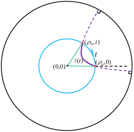
Figure 1: The circular blue line denotes the time evolution, the purple line, which is perpendicular to the hyperbolic boundary denoted by the black circle, is the hyperbolic geodesic connecting the starting and ending points.

and substituting into (2.45), we can get the corresponding spread complexity

$$C(t)=C_{z\to ze^{-\text{i}t}} = h(\cosh\ell(t)-1)=h(\cosh^{2}\theta-\sinh^{2}\theta\cos t-1),$$ (2.49)

$$= 2h\sinh^{2}\theta\sin^{2}\frac{t}{2},\quad z\equiv\tanh\frac{\theta}{2},$$ (2.50)

where we have used the hyperbolic law of cosines. Alternatively, one can obtain the same result from (2.27) by substituting

$$\begin{pmatrix}A&B\\ C&D\end{pmatrix}=\left(\begin{array}[]{cc}\cosh\left(\frac{\theta}{2}\right)&\sinh\left(\frac{\theta}{2}\right)\\ \sinh\left(\frac{\theta}{2}\right)&\cosh\left(\frac{\theta}{2}\right)\\ \end{array}\right),$$ (2.53)

$$\frac{\langle\psi(t)|L_{0}|\psi(t)\rangle}{\langle\psi(t)|\psi(t)\rangle}=\frac{\langle\psi_{0}|L_{0}|\psi_{0}\rangle}{\langle\psi_{0}|\psi_{0}\rangle}=h\cosh\theta,$$ (2.54)

$$\frac{\langle\psi(t)|L_{\pm 1}|\psi(t)\rangle}{\langle\psi(t)|\psi(t)\rangle}=e^{\mp\text{i}t}\frac{\langle\psi_{0}|L_{\pm 1}|\psi_{0}\rangle}{\langle\psi_{0}|\psi_{0}\rangle}=e^{\mp\text{i}t}h\sinh\theta,$$ (2.55)

where we have used the identities

$$e^{\text{i}L_{0}t}L_{\pm}e^{-\text{i}L_{0}t}=e^{\mp\text{i}t}L_{\pm}.$$ (2.56)

This result of spread complexity (2.50) matches the one derived in [1] from the mapping method. Note that our proposal provides a simple geometric approach for computing Krylov complexity under any $SL(2,\mathbb{R})$ flows.

2.3 The holographic description

In the semi-classical regime where $h\gg 1$ but $h\ll\frac{1}{G_{N}}$, the primary operator is dual to a probe free massive particle. Let us first determine the holographic description of the initial state $|\psi_{0}\rangle=\mathcal{O}(z_{0})|\Omega\rangle$. In the bulk, this state is also prepared by a Euclidean path integral from $t=-\infty$ to $t=0$. Since we neglect the backreaction of the particle, the spacetime remains the (Euclidean) global AdS₃. In the semi-classical regime, the path integral of the particle can be approximated by the contribution of the classical saddle point, namely the geodesic. To complete the spacetime from $t=-\infty$ to $t=\infty$, we consider the density matrix $\rho=|\psi_{0}\rangle\langle\psi_{0}\rangle=\mathcal{O}|\Omega\rangle\langle\Omega|\mathcal{O}^{\dagger}$. Therefore, the dual gravity solution of the density matrix $|\psi_{0}\rangle\langle\psi_{0}|$ is the Euclidean global AdS₃ spacetime with a massive particle propagating from the boundary point $z=z_{0}$ to another $z_{0}=1/z_{0}^{*}$. By exploiting the spacetime isometry, we can also always set $z_{0}$ to be real without loss of generality. The geodesic connecting these two points in Euclidean global AdS₃ is given by

$$\tanh\rho=\tanh\rho_{0}\cosh t_{E},$$ (2.57)

with

$$z_{0}=\tanh\frac{\rho_{0}}{2}.$$ (2.58)

Therefore, the state $|\psi_{0}\rangle$ is dual to a massive particle located at the position $\rho=\rho_{0}$ on the $t=0$ Cauchy slice. To obtain the time-evolved state $|\psi(t)\rangle$, we replace the upper half of Euclidean AdS₃, which is dual to $\langle\psi_{0}|$, with the corresponding Lorentzian spacetime. The entire construction is illustrated in Figure 2.

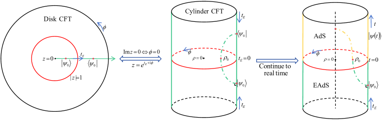
Figure 2: Depiction of the holographic construction of the quantum state $|\psi(t)\rangle$.

In conclusion, the state $|\psi(t)\rangle$ is dual to the geodesic trajectory

$$\tanh\rho=\tanh\rho_{0}\cos t,\quad t\geq 0.$$ (2.59)

Note that the relation (2.58) is identical to (2.50), and the reduced metric at the $t=0$ slice is

$$ds_{t=0}^{2}=d\rho^{2}+\sinh^{2}\rho d\phi^{2}$$ (2.60)

which matches (2.44) upon identifying $\rho=\theta$ and $\phi=u$. This identification suggests that the state distance is indeed related to a physical spacetime distance via (2.45). It should be noted that a similar correspondence between timelike geodesics in AdS and quantum circuits (states) has been proposed in [55].

We have shown that the spread complexity is given by (2.27), which takes the form of a linear combination of the expectation values of the $SL(2,\mathbb{R})$ generators. The conformal transformations generated by these generators can be lifted to the isometric transformations in the AdS spacetime, associated with the Killing vector fields $\hat{L}_{n}$ corresponding to the generators $L_{n}$ [56, 57]. One important feature of Killing vectors is that they give rise to conserved quantities along geodesics:

$$\hat{Q}_{n}=\hat{L}_{n}^{\alpha}\hat{u}_{\alpha},\quad\frac{d}{d\tau}\hat{Q}_{n}=0,$$ (2.61)

where $\hat{u}$ and $\tau$ denote the tangent vector and affine parameter of the geodesic, respectively. Therefore, the expectation values of the symmetry generators are naturally related to the corresponding conserved charges. In the global AdS₃ spacetime, described by the metric (2.1), the Killing vectors are explicitely given by

$$\hat{L}_{0}=\partial_{t}+\partial_{\phi},$$ (2.62)

$$\hat{L}_{\pm 1}=e^{\pm\text{i}(t+\phi)}\left(\tanh\rho\partial_{t}+\coth\rho\partial_{\phi}\mp\text{i}\partial_{\rho}\right),$$ (2.63)

and the tangent vector of geodesic (2.59) is

$$\hat{u}_{\phi}=0,\quad\hat{u}_{t}=-\cosh\rho_{0},\quad\hat{u}_{\rho}=-\sin t\sinh\rho_{0}.$$ (2.64)

Indeed, we find the following relations:

$$\frac{\langle\psi(t)|L_{0}|\psi(t)\rangle}{\langle\psi(t)|\psi(t)\rangle} = h\cosh\rho_{0}=-h\hat{Q}_{0},$$ (2.65)

$$\frac{\langle\psi(t)|L_{\pm}|\psi(t)\rangle}{\langle\psi(t)|\psi(t)\rangle} = e^{\mp\text{i}t}h\sinh\rho_{0}=-e^{\mp\text{i}t}h\hat{Q}_{\pm}.$$ (2.66)

Recall that the tangent vector (2.64), which also serves as the velocity vector of the free particle, is proportional to the canonical momentum of the particle: $p_{\alpha}=h\hat{u}_{\alpha}$. Substituting (2.53)-(2.55) and setting $\theta=\rho_{0}$ into (2.27), we find

$$\mathcal{L}_{0}=\cosh\rho_{0}L_{0}-\sinh\rho_{0}\frac{L_{+1}+L_{-1}}{2},$$ (2.67)

such that the spread complexity can be written compactly as

$$C(t)+h=\hat{e}_{0}^{\alpha}p_{\alpha},$$ (2.68)

where

$$\hat{e}_{0} = -\left(\cosh\rho_{0}\hat{L}_{0}+e^{-\text{i}t}\hat{L}_{+1}+e^{\text{i}t}\hat{L}_{-1}\right)=(\sinh\rho_{0}\cos\phi\tanh\rho-\cosh\rho_{0})\partial_{t}$$

$$+ (\sinh\rho_{0}\cos\phi\coth\rho-\cosh\rho_{0})\partial_{\phi}+\sinh\rho_{0}\sin\phi\partial_{\rho},$$

$$\hat{e}_{0}^{\alpha}\hat{e}_{0,\alpha} = -1.$$ (2.69)

The expressions (2.68) and (2.69) suggest that the spread complexity can be interpreted as the energy of the particle measured by an observer moving along the timelike vector $\hat{e}_{0}$. Furthermore, except for $\hat{e}_{0}$ we can associate the observer with other two local Lorentz orthonormal frames (tetrad):

$$\hat{e}_{1} = (\cosh\rho_{0}\cos\phi\tanh\rho-\sinh\rho_{0})\partial_{t}$$ (2.70)

$$+ (\cosh\rho_{0}\cos\phi\coth\rho-\sinh\rho_{0})\partial_{\phi}+\cosh\rho_{0}\sin\phi\partial_{\rho},$$

$$\hat{e}_{\rho} = \tanh\rho\sin\phi\partial_{t}+\coth\rho\sin\phi\partial_{\phi}-\cos\phi\partial_{\rho}.$$ (2.71)

The components of the measured momentum are then:

$$P_{0} =\hat{e}_{0}\cdot\hat{p}=h(\cosh^{2}\rho_{0}-\sinh^{2}\rho_{0}\cos t),$$ (2.72)

$$P_{1} =\hat{e}_{1}\cdot\hat{p}=h\sinh(2\rho_{0})\sin^{2}\frac{t}{2},$$ (2.73)

$$P_{\rho} =\hat{e}_{\rho}\cdot\hat{p}=-h\sinh\rho_{0}\sin t.$$ (2.74)

This constitutes the main result of our work. Although our proposal is based on several simple observations, (2.23), (2.68), and (2.69), this interpretation is conceptually appealing. First, it provides a novel understanding of the ambiguity in spread complexity: from a holographic perspective, since spread complexity is a measured quantity, its value naturally depends on the observer. This reflects a fundamental principle of relativity. Second, the interpretation endows spread complexity with an operational meaning. Analogous to quantum complexity, we can imagine that the quantum state is being manipulated by an experimentalist, whose reference frame determines the measurement outcome. Last but not least, one of the fundamental features of quantum state complexity is its inherent ambiguity, as previously noted. This poses a challenge for its holographic description. A promising interpretation of this ambiguity is the so-called “complexity = anything” prescription [11, 12, 58], which suggests that there exist infinitely many gravitational quantities behaving analogously to quantum complexity. However, how to match these gravitational observables with the ambiguities in quantum complexity remains unclear. In contrast, for Krylov complexity, we propose a different explanation by connecting the ambiguity in relativity (observer dependence) with the ambiguity in quantum mechanics (reference and gate-set dependence).

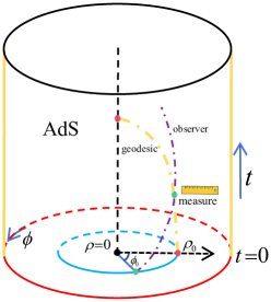
Figure 3: Illustration of our proposal: A specific observer interacts with the dual particle and performs a measurement. The spread complexity corresponds to the measured energy, while the complexity rate is identified with the radial momentum observed by that observer.

Next, we derive the correspondence proposed in [1], which states that the spread complexity rate is proportional to the (proper) radial momentum:

$$\frac{dC(t)}{dt}\propto p_{\rho}.$$ (2.75)

Starting from (2.25) and (2.67), we can derive the complexity rate

$$\frac{dC(t)}{dt}=\text{i}\frac{\langle\psi(t)|[L_{0},\mathcal{L}_{0}]|\psi(t)\rangle}{\langle\psi(t)|\psi(t)\rangle}=\sinh\rho_{0}\frac{\langle\psi(t)|\frac{\text{i}}{2}(L_{+1}-L_{-1})|\psi(t)\rangle}{\langle\psi(t)|\psi(t)\rangle}.$$ (2.76)

Following our earlier argument, the operator $\frac{\text{i}}{2}(L_{+}-L_{-})$, which coincides with the radial momentum operator introduced in [59], corresponds to the vector field

$$-\frac{\text{i}}{2}(e^{-\text{i}t}\hat{L}_{+1}+e^{\text{i}t}\hat{L}_{-1})=-\hat{e}_{\rho}.$$ (2.77)

Therefore, we immediately find that the complexity rate is proportional to the measured radial momentum:

$$\frac{dC(t)}{dt}=-\sinh\rho_{0}\hat{e}_{\rho}^{\alpha}p_{\alpha}=-\sinh\rho_{0}p_{\rho},$$ (2.78)

where $p_{\rho}=P_{\rho}$ is a coincidence due to the specific choice of the radial coordinate. It should be pointed out that there is a subtlety in the correspondence between the complexity rate and radial momentum. The radial momentum itself is not invariant under redefinitions of the radial coordinate, which raises the question: which radial coordinate should be used? In [1] (see also [41, 42]), the radial coordinate is chosen such that the radial momentum coincides with the complexity rate. This appears somewhat circular and ad hoc. In contrast, our framework provides an invariant quantity—the measured radial momentum—that is independent of the choice of radial coordinate.

By studying this simple holographic model in detail, we have presented the important ingredients of our proposal: the state distance, which provides a geometric interpretation for the spread complexity, and an observer, which dictates the choice of the Krylov basis. Next, we show how to apply our proposal to obtain results in other AdS spacetimes without really trying.

3 The Poincar$\acute{\text{e}}$ AdS₃

The metric of the Poincar$\acute{\text{e}}$ AdS₃ spacetime is given by

$$ds^{2}=\frac{-dT^{2}+dX^{2}+dZ^{2}}{Z^{2}},$$ (3.1)

which is related to the global AdS₃ metric (2.1) via the following coordinate transformaitons:

$$Z = \frac{1}{\sinh(\rho)\cos(\phi)+\cosh(\rho)\cos(t)},$$

$$X = Z\sinh\rho\sin\phi,$$ (3.2)

$$T = Z\cosh\rho\sin t.$$

To study the dual CFT, we perform a Wick rotation of the time coordinate $T=-\text{i}T_{E}$ and introduce holomorphic and anti-holomorphic coordinates:

$$\xi=T_{E}+\text{i}X,\quad\bar{\xi}=T_{E}-\text{i}X.$$ (3.3)

The coordinate transformations (3.2) imply the conformal map between the global CFT and the Poincar$\acute{\text{e}}$ CFT:

$$z=\frac{1+\xi}{1-\xi},\quad\xi=\frac{z-1}{z+1},$$ (3.4)

under which the hyperbolic plane becomes the Poincar$\acute{\text{e}}$ half-plane with the metric

$$ds^{2}=4\frac{d\xi d\bar{\xi}}{(\xi+\bar{\xi})^{2}}=\frac{dT_{E}^{2}+dX^{2}}{T_{E}^{2}}.$$ (3.5)

The length of the geodesic connecting arbitary points $P_{1}=(T_{E,1},X_{1})$ and $P_{2}=(T_{E,2},X_{2})$ is given by

$$\ell_{12}=2\text{arcsinh}\frac{|P_{1}-P_{2}|}{2\sqrt{T_{E,1}T_{E,2}}}.$$ (3.6)

Using the relation (2.45), we immediately obtain the state distance in Poincar$\acute{\text{e}}$ CFT:

$$\mathfrak{d}=h(\cosh\ell_{12}-1)=h\frac{(T_{E,1}-T_{E,2})^{2}+(X_{1}-X_{2})^{2}}{2T_{E,1}T_{E,2}}.$$ (3.7)

The states in the Poincar$\acute{\text{e}}$ CFT are obtained via a Euclidean path integral from $T_{E}=-\infty$ to $T_{E}=0$, which corresponds to the the unit disk in the $z$ coordinates. Without loss of generality, suppose the operator is initially inserted at $\xi=\xi_{0}$, preparing the state:

$$|\psi_{0}\rangle=\mathcal{O}(\xi_{0}=-T_{E,0})|\Omega\rangle,\quad T_{E,0}>0.$$ (3.8)

The Lorentzian time evolution is $\xi=\xi_{0}+\text{i}T$, so the spread complexity and its rate becomes:

$$C(T)=\mathfrak{d}(\xi_{0},\xi_{0}+\text{i}T)=\frac{T^{2}}{2T_{E,0}^{2}},\quad\frac{dC(T)}{dT}=\frac{T}{T_{E,0}},$$ (3.9)

which exactly matches the result derived in [1]. It is important to note that this result cannot be obtained simply by applying the coordinate transformation (3.2) to (2.50). The reason lies in the fact that the Hamiltonian in the Poincar$\acute{\text{e}}$ spacetime is generated by $H_{\text{Poincar$\acute{\text{e}}$ }}=L_{-1}^{P}+\bar{L}_{-1}^{P}$, where the $SL(2,R)$ generators are defined as

$$L_{n}^{P}=\int_{-\text{i}\infty}^{\text{i}\infty}\frac{d\xi}{2\pi\text{i}}\xi^{n+1}T(\xi),$$ (3.10)

and their relation to the global $SL(2,\mathbb{R})$ generators can be derived by substituting into the conformal transformation (3.4):

$$L_{n}^{P}=\oint dz\frac{(z+1)^{2}}{2}\left(\frac{z-1}{z+1}\right)^{n+1}T(z),$$ (3.11)

Explicitly, the relations between the two sets of generators are:

$$L_{0}^{P}=\frac{L_{+1}-L_{-1}}{2},\quad L_{\pm 1}^{P}=\mp L_{0}+\frac{L_{+1}+L_{-1}}{2},$$ (3.12)

$$L_{0}=-\frac{L_{+1}^{P}-L_{-1}^{P}}{2},\quad L_{\pm 1}=\pm L_{0}^{P}+\frac{L_{+1}^{P}+L_{-1}^{P}}{2}.$$ (3.13)

Now, let us present the holographic description. The conjugate of the initial state (3.8) is

$$\langle\psi_{0}|=\langle\Omega|\mathcal{O}(\xi=T_{E,0}),$$ (3.14)

and as previously discussed, the density matrix $|\psi_{0}\rangle\langle\psi_{0}|$ is dual to the Euclidean Poincar$\acute{\text{e}}$ spacetime with a massive particle propagating along the Euclidean geodesic

$$Z^{2}+T_{E}^{2}=T_{E,0}^{2}\,.$$ (3.15)

Furthermore, the time-evolued state $|\psi(t)\rangle=e^{\text{i}L_{-1}^{P}t}|\psi_{0}\rangle$ is dual to the Lorenzian geodesic

$$Z^{2}-T^{2}=T_{E,0}^{2},\quad T\geq 0,$$ (3.16)

with tangent vector $\hat{u}=(u^{T},u^{X},u^{Z})$ and momentum components:

$$u^{T}=\frac{T^{2}+T_{E,0}^{2}}{T_{E,0}},\quad u^{X}=0,\quad u^{Z}=\frac{T\sqrt{T^{2}+T_{E,0}^{2}}}{T_{E,0}},$$ (3.17)

$$p_{T}=-\frac{h}{T_{E,0}},\quad p_{X}=0,\quad p_{Z}=\frac{hT}{T_{E,0}\sqrt{T^{2}+T_{E,0}^{2}}}.$$ (3.18)

The generators $L_{n}^{P}$ correspond to the following (normalized) Killing vectors

$$\hat{L}_{0}^{P}=\text{i}\left((T+X)(\partial_{T}+\partial_{X})+Z\partial_{Z}\right),$$ (3.19)

$$\hat{L}_{-1}^{P}=\partial_{T}+\partial_{X},$$ (3.20)

$$\hat{L}_{+1}^{P}=-\left((T+X)^{2}+Z^{2}\right)\partial_{T}-\left((T+X)^{2}-Z^{2}\right)\partial_{X}-2(T+X)Z\partial_{Z}.$$ (3.21)

Similarly, we find that the relations between the conserved charges associated with these Killing vectors and the expectation values of the corresponding generators are:

$$\frac{\langle\psi(t)|L^{P}_{0}|\psi(t)\rangle}{\langle\psi(t)|\psi(t)\rangle} = -h\frac{\text{i}T}{T_{E,0}}=-h\,\text{i}T\hat{Q}_{-1},$$ (3.22)

$$\frac{\langle\psi(t)|L^{P}_{+1}|\psi(t)\rangle}{\langle\psi(t)|\psi(t)\rangle} = hT^{2}\hat{Q}_{-1}-h\hat{Q}_{+1},$$ (3.23)

$$\frac{\langle\psi(t)|L^{P}_{-1}|\psi(t)\rangle}{\langle\psi(t)|\psi(t)\rangle} = -h\hat{Q}_{-1}.$$ (3.24)

It is convenient to compute the expectation values of the generators using the original $z$ coordinates. For example,

$$\frac{\langle\psi(t)|L^{P}_{-1}|\psi(t)\rangle}{\langle\psi(t)|\psi(t)\rangle}=\frac{\langle\psi_{0}|L^{P}_{-1}|\psi_{0}\rangle}{\langle\psi_{0}|\psi_{0}\rangle}=\langle\mathcal{O}(z_{0})(L_{0}+\frac{L_{+1}+L_{-1}}{2})\mathcal{O}(z_{0})\rangle=\frac{1}{T_{E,0}},$$ (3.25)

where $z_{0}=\frac{1-T_{E,0}}{1+T_{E,0}}$. In the last section, we have shown that for the state $|\psi_{0}\rangle=\mathcal{O}(z_{0}=\tanh\frac{\rho_{0}}{2})|\Omega\rangle$, the spread complexity is determined by the generator

$$\mathcal{L}_{0}=\cosh\rho_{0}L_{0}-\frac{1}{2}\sinh\rho_{0}(L_{+1}+L_{-1}).$$ (3.26)

Transforming into the Poincar$\acute{\text{e}}$ coordinates, we obtain

$$\mathcal{L}_{0}^{P}=-\frac{1}{2}\left(\frac{L_{+1}^{P}}{{T_{E,0}}}-{T_{E,0}}L^{P}_{-1}\right)$$ (3.27)

and the spread complexity can be written as

$$C(T)=\hat{e}_{0}^{\alpha}p_{\alpha}-h=\frac{T^{2}}{2T_{E,0}^{2}},\quad\hat{e}_{0}^{\alpha}\hat{e}_{0,\alpha}=-1,$$ (3.28)

$$\hat{e}_{0}=\frac{1}{2}\left(\frac{\hat{L}_{+1}^{P}-2\text{i}T\hat{L}_{0}^{P}-T^{2}\hat{L}_{-1}^{P}}{T_{E,0}}-T_{E,0}\hat{L}_{-1}^{P}\right)$$

$$\quad=-\frac{T_{E,0}^{2}+X^{2}+Z^{2}}{2T_{E,0}}\partial_{T}-\frac{T_{E,0}^{2}+X^{2}-Z^{2}}{2T_{E,0}}\partial_{X}-\frac{XZ}{T_{E,0}}\partial_{Z},$$ (3.29)

The spread complexity rate is then given by

$$\frac{dC(T)}{dT}=\text{i}\frac{\langle\psi(t)|[L_{-1}^{P},\mathcal{L}_{0}^{P}]|\psi(t)\rangle}{\langle\psi(t)|\psi(t)\rangle}=\frac{\text{i}}{T_{E,0}}\frac{\langle\psi(t)|L_{0}^{P}|\psi(t)\rangle}{\langle\psi_{0}|\psi_{0}\rangle}=\frac{\text{i}}{T_{E,0}}\frac{\langle\psi_{0}|L_{0}^{P}-\text{i}TL_{-1}^{P}|\psi_{0}\rangle}{\langle\psi_{0}|\psi_{0}\rangle}.$$ (3.30)

Since the operator $\text{i}(L_{0}^{P}-\text{i}TL_{-1}^{P})$ corresponds to the combination of the Killing vector

$$-\text{i}(\hat{L}_{0}^{P}-\text{i}T\hat{L}_{-1}^{P})=X(\partial_{T}+\partial_{X})+Z\partial_{Z}=\hat{e}_{Z},\quad\hat{e}_{Z}^{\alpha}\hat{e}_{Z,\alpha}=1,\quad\hat{e}_{Z}^{\alpha}\hat{e}_{0,\alpha}=0,$$ (3.31)

We find that the complexity rate is proportional to the measured radial momentum:

$$\frac{dC(T)}{dT}=\frac{\hat{e}^{\alpha}_{Z}p_{\alpha}}{T_{E,0}}=\frac{Z}{T_{E,0}}p_{Z},$$ (3.32)

rather than the canonical momentum $p_{Z}$. We emphasize again that the fact $\hat{e}^{\alpha}_{Z}p_{\alpha}\neq p_{Z}$ simply reflects the coordinate choice. In terms of the proper radial coordinate the Poincar$\acute{\text{e}}$ AdS metric becomes

$$ds^{2}=d\rho^{2}+e^{2\rho}(-dT^{2}+dX^{2}),$$ (3.33)

the radial vector becomes $\hat{e}_{\rho}=X(\partial_{T}+\partial_{X})-\partial_{\rho}$ with the measured radial momentum equal to the (opposite of) proper radial momentum:

$$P_{\rho}=\hat{e}_{\rho}^{\mu}p_{\mu}=-p_{\rho},$$ (3.34)

as proposed in [1]. Therefore, our proposal explains why the proper radial momentum proposal gives the correct result for the complexity rate.

4 The Rindler AdS₃

The Rindler spacetime (also known as the decompactified BTZ black hole) consists of four distinct wedges. Since our arguments rely primarily on the isometries of the spacetime, we expect that the results obtained in the Rindler spacetime will carry over directly to the (single-sided) BTZ black hole. We will insert the operator in the right wedge, where the metric is given by

$$ds^{2} =-\sinh^{2}\rho_{r}dt_{r}^{2}+d\rho_{r}^{2}+\cosh^{2}\rho_{r}d\phi_{r}^{2},$$ (4.1)

$$\rho_{r} >0,\quad-\infty<t_{r}<\infty,\quad-\infty<\phi_{r}<\infty.$$ (4.2)

The left wedge can be obtained from the right one via the analytic continuation $t_{l}=-t_{r}+\text{i}\pi,\,\phi_{l}=-\phi_{r}$. The Rindler space is dual to the thermofield double state $\Psi_{\text{TFD}}$, which is invariant under the combined $SL(2,\mathbb{R})$ transformations:

$$L_{n}^{R}|\Psi_{\text{TFD}}\rangle=(L_{n}^{r}-(-1)^{n}L_{-n}^{l})|\Psi_{\text{TFD}}\rangle=0.$$ (4.3)

Since the operator is inserted only in the right wedge, its dynamics in the left wedge are trivial. Therefore, we only need to restrict our attention to the right wedge. The coordinate transformations between global AdS and the right wedge of Rindler space are:

$$\cosh\rho\cos t=\cosh\rho_{r}\cosh\phi_{r},\quad\cosh\rho\sin t=\sinh\rho_{r}\sinh t_{r},$$ (4.4)

$$\sinh\rho\sin\phi=\cosh\rho_{r}\sinh\phi_{r},\quad\sinh\rho\cos\phi=\sinh\rho_{r}\cosh t_{r}.$$ (4.5)

Similarly, we define an Euclidean coordinate on the boundary of the Rindler spacetime as [60]

$$\zeta=e^{\phi_{r}-\text{i}\tau_{r}},$$ (4.6)

where $\tau_{r,l}=\text{i}t_{r,l}$. These coordinate transformations imply the conformal map

$$z=-\text{i}\frac{1+\text{i}\zeta}{1-\text{i}\zeta},\quad\zeta=\text{i}\frac{1-\text{i}z}{1+\text{i}z}.$$ (4.7)

They also yield the following relations between the $SL(2,\mathbb{R})$ generators [60]:

$$L_{0}=-\text{i}\frac{L_{+1}^{R}+L_{-1}^{R}}{2},\quad L_{\pm 1}=-\text{i}L_{0}^{R}\pm\frac{L_{+1}^{R}-L_{-1}^{R}}{2},$$ (4.8)

$$L_{0}^{R}=\text{i}\frac{L_{+1}+L_{-1}}{2},\quad L_{\pm 1}^{R}=\text{i}L_{0}\pm\frac{L_{+1}-L_{-1}}{2}.$$ (4.9)

Note that $L_{n}^{R}$ are anti-Hermitian operators, and the Rindler Hamiltonian is given by $H^{\text{Rindler}}=-\text{i}(L_{0}^{R}-\bar{L}_{0}^{R})$. In the $\zeta$ coordinates, the hyperbolic plane has the metric

$$ds^{2}=-\frac{4d\zeta d\bar{\zeta}}{(\zeta-\bar{\zeta})^{2}}.$$ (4.10)

It is convenient to introduce a new variable

$$\zeta=e^{\phi_{r}}\frac{\text{i}+e^{\theta_{r}}}{-\text{i}+e^{\theta_{r}}},$$ (4.11)

which allows us to rewrite the metric in a more familiar form:

$$ds^{2}=d\theta_{r}^{2}+\cosh\theta_{r}d\phi_{r}^{2}.$$ (4.12)

The length of the geodesic connecting arbitary two points $P_{1}=(\theta_{r,1},\phi_{r,1})$ and $P_{2}=(\theta_{r,2},\phi_{r,2})$ is given by

$$\ell_{12}=\text{arccosh}\left(\cosh\theta_{r,1}\cosh\theta_{r,2}\cosh(\phi_{r,2}-\phi_{r,1})-\sinh\theta_{r,1}\sinh\theta_{r,2}\right)$$ (4.13)

and the corresponding state distance becomes

$$\mathfrak{d}=h(\cosh\ell_{12}-1)=h\left(\left(\cosh\theta_{r,1}\cosh\theta_{r,2}\cosh(\phi_{r,2}-\phi_{r,1})-\sinh\theta_{r,1}\sinh\theta_{r,2}\right)-1\right)$$ (4.14)

Under the Lorentzian time evolution $(\theta_{r,0},\phi_{r,0})\to(\theta_{r,0},\phi_{r,0}+t_{r})$, the spread complexity and the its rate become:

$$C(t_{r})=h(\cosh\theta_{r,0}^{2}\cosh t_{r}-\sinh^{2}\theta_{r,0}-1),\quad\frac{dC(t_{r})}{dt_{r}}=h\cosh\theta_{r,0}^{2}\sinh t_{r}\,.$$ (4.15)

Without loss of the generality, we can set $\phi_{r,0}=0$, so the initial state is

$$|\psi_{0}\rangle=\mathcal{O}(\theta_{r,0})|\Psi_{\text{TFD}}\rangle.$$ (4.16)

Following previous arguments, we can find that time-evolved state $|\psi(t)\rangle$ is dual to the geodesic

$$\tanh\rho_{r}\cosh t_{r}=\tanh\rho_{0},\quad\rho_{0}=\theta_{r,0},\quad t_{r}\geq 0.$$ (4.17)

As in the global spacetime, identifying $\rho_{0}=\theta_{r,0}$ suggests that the hyperbolic space (4.12) can be identified with the $t_{r}=0$ time slice. The tangent vector along this geodesic and the associated momentum are:

$$\hat{u} = \sinh\rho_{0}(\coth^{2}\rho_{0}\cosh^{2}t_{r}-1)\partial_{t_{r}}-\cosh\rho_{0}\sinh t_{r}\partial_{\rho},$$ (4.18)

$$p_{t_{r}} = -h\sinh^{2}\rho_{0},\quad p_{\phi_{r}}=0,\quad p_{\rho}=-h\cosh\rho_{0}\sinh t_{r}.$$ (4.19)

In the right wedge of the Rindler space, the (normalized) Killing vectors are

$$\hat{L}_{0}^{r} = -\text{i}(\partial_{t_{r}}+\partial_{\phi_{r}}),$$ (4.20)

$$\hat{L}_{\pm 1}^{r} = -\text{i}e^{t_{r}+\phi_{r}}(\cosh\rho\partial_{t_{r}}+\tanh\rho\partial_{\phi_{r}}\mp\partial_{\rho}),$$ (4.21)

and the conserved charges associated with these Killing vectors relate to the expectation values of the corresponding generators as follows:

$$\frac{\langle\psi(t)|L^{r}_{0}|\psi(t)\rangle}{\langle\psi(t)|\psi(t)\rangle} = \text{i}h\sinh\rho_{0}=h\hat{Q}_{0},$$ (4.22)

$$\frac{\langle\psi(t)|L^{r}_{\pm}|\psi(t)\rangle}{\langle\psi(t)|\psi(t)\rangle} = e^{\mp t_{r}}h\cosh\rho_{0}=he^{\mp t_{r}}\hat{Q}_{\pm}.$$ (4.23)

Substituting (4.8) into the expression for (2.67) and retaining only the right-wedge components, we find that the spread complexity corresponds to the generator

$$\mathcal{L}^{r}_{0}=\text{i}(\sinh\rho_{0}L_{0}^{r}-\cosh\rho_{0}\frac{L_{+1}^{r}+L_{-1}^{r}}{2})\,.$$ (4.24)

which leads to

$$C(t)+h=\hat{e}_{0}^{\alpha}p_{\alpha}=h\left(\cosh^{2}\rho_{0}\cosh t_{r}-\sinh^{2}\rho_{0}\right),\quad\hat{e}_{0}^{\alpha}\hat{e}_{0,\alpha}=-1,$$ (4.27)

$$\hat{e}_{0}=\text{i}(\sinh\rho_{0}\hat{L}_{0}^{r}-\cosh\rho_{0}\frac{e^{-t_{r}}\hat{L}^{r}_{+1}+e^{t_{r}}\hat{L}^{r}_{-1}}{2}),$$

$$= -(\cosh\rho_{0}\coth\rho\cosh\phi_{r}+\sinh\rho_{0})\partial_{t_{r}}+(\sinh\rho_{0}-\cosh\rho_{0}\tanh\rho\cosh\phi_{r})$$

$$+\cosh\rho_{0}\sinh\phi_{r}\partial_{\rho}.$$

Similarly, we find that the complexity rate is given by

$$\frac{dC(t_{r})}{dt}=\frac{\langle\psi(t)|[L^{r}_{0},\mathcal{L}^{r}_{0}]|\psi(t)\rangle}{\langle\psi(t)|\psi(t)\rangle}=\cosh\rho_{0}\frac{\langle\psi(t)|\text{i}\frac{L_{-1}^{r}-L_{+1}^{r}}{2}|\psi(t)\rangle}{\langle\psi(t)|\psi(t)\rangle}.$$ (4.28)

Using the fact that the operator $\text{i}\frac{L_{-1}^{r}-L_{+1}^{r}}{2}$ corresponds to the linear combination the Killing vectors:

$$\hat{e}_{\rho} = \frac{\text{i}}{2}\left(e^{t_{r}}\hat{L}_{-1}-e^{-t_{r}}\hat{L}_{+1}\right)$$ (4.29)

$$= \sinh\phi_{r}(\coth\rho\partial_{t_{r}}+\tanh\rho\partial_{\phi_{r}})-\cosh\phi_{\phi_{r}}\partial_{\rho},$$ (4.30)

we get

$$\frac{dC(t_{r})}{dt}=\cosh\rho_{0}\hat{e}_{\rho}^{\alpha}p_{\alpha}=-\cosh\rho_{0}p_{\rho},$$ (4.31)

which matches the result found in [1].

5 Conclusions and Outlooks

In this work, we proposed a holographic description of the spread complexity and its rate in 2D CFTs. By leveraging the underlying symmetries, we explicitly constructed the Krylov basis, which turns out not to be unique, giving rise to ambiguities in spread complexities. This ambiguity closely mirrors that of quantum complexity. To describe the spread complexity under general $SL(2,\mathbb{R})$ flows, we introduced the notions of distance complexity and state distance, providing a novel geometric interpretation of the spread complexity and connecting it to Nielsen’s complexity. Within the AdS/CFT correspondence, we related the expectation values of the $SL(2,\mathbb{R})$ charges to the conserved quantities associated with the corresponding Killing vectors. Remarkably, the spread complexity can be expressed as the energy measured by an observer moving along the worldline defined by $\hat{e}_{0}$, as shown in eq. (2.68). Holographically, the ambiguity in spread complexity is interpreted as an observer dependence, a feature rooted in relativity. Furthermore, the complexity rate is identified with the measured radial momentum, which remains invariant under redefinitions of the radial coordinate. Below, we outline several open issues and potential directions for future research.

First, throughout this work, we have focused on the semi-classical regime where the conformal dimension $h$ of the primary operator is in the range of $\frac{1}{G_{N}}\gg h\gg 1$. In this limit, the dual state corresponds to a massive particle propagating along a geodesic in an unperturbed AdS spacetime. When $h\ll 1$, the primary operator should instead be dual to a free bulk scalar field, and the time-evolved state $|\psi(t)\rangle$ is described by the wavefunction $\Psi(\rho,t,\phi)=\langle\hat{\phi}(\rho,t,\phi)|\psi(t)\rangle$. In this regime, we expect the conserved charges $\hat{Q}_{n}$ to be replaced by appropriate bulk expectation values such as $\langle\Psi^{*},\hat{L}_{n}^{\mu}\partial_{\mu}\Psi\rangle$, while the spread complexity may still admit an interpretation as the field energy measured by a given observer. For $h\sim\frac{1}{G_{N}}$, we can still treat the primary operator as a massive particle, but the backreaction of the particle becomes non-negligible. The resulting geometry develops conical singularities around the worldline of the particle. When the particle is at rest at the center of the global AdS₃, the bulk solution corresponds to the conical AdS₃ spacetime. For off-center static particles, recent studies suggest that the dual geometry can be described by a three-dimensional C-metric [61, 62, 63, 64, 65, 66, 67, 68, 69]. In the case of a moving particle, the dual geometry has been argued to correspond to a locally quenched spacetime [47]. Importantly, all these geometries are related to global AdS₃ via coordinate transformations. Therefore, the worldline of the observer can be extended to these more general settings. A potentially related work is [70].

Second, The correspondence between conformal symmetry generators and Killing vectors extends naturally to higher dimensions. Thus, our proposal is expected to generalize to higher-dimensional AdS spacetimes. Consider the AdS_d+1 metric

$$ds^{2}=-\cosh^{2}\rho dt^{2}+d\rho^{2}+\sinh^{2}\rho d\vec{x}^{2},$$ (5.1)

where $\vec{x}^{2}=1$ parameterizes the sphere $S^{d-1}$. The boundary CFT lives on $\mathbb{R}\times S^{d-1}$. Performing a Wick rotation $t\to-\text{i}\tau$, the conformal symmetry of the CFT is described by the group $SO(1,d+1)$. We denote the generators of $SO(1,d+1)$ as $L_{ab},\,,a,b=-1,0,\dots,d$, acting in the embedding space $\mathbb{R}^{1,d+1}$. These relate to the “physical” generators in the CFT as follows;

$$L_{\mu\nu}=M_{\mu\nu},\quad L_{-1,0}=D,\quad L_{0,\mu}=\frac{1}{2}(P_{\mu}+K_{\mu}),\quad L_{-1,\mu}=\frac{1}{2}(P_{\mu}-K_{\mu}).$$ (5.2)

The time-evolved state can be written as

$$|\psi(t)\rangle=e^{-\text{i}Dt}\mathcal{O}(\tau_{0},\vec{x}_{0})|\Omega\rangle=e^{-\text{i}Dt}e^{\rho x^{a}(P_{a}-K_{a})}\mathcal{O}(0)|\Omega\rangle$$ (5.3)

where $\rho$ is determined by $\tau_{0}$. As in the 2D case, the $\mathcal{O}(\tau_{0},\vec{x}_{0})|\Omega\rangle$ defines a primary state of the generator defined by

$$\mathcal{L}_{0}=e^{\rho x^{a}(P_{a}-K_{a})}De^{-\rho x^{a}(P_{a}-K_{a})}.$$ (5.4)

Noting that $\{D,x^{a}P_{a},x^{a}K_{a}\}$ forms a $\mathfrak{sl}_{2}$ algebra, we find

$$e^{\rho x^{a}(P_{a}-K_{a})}De^{-\rho x^{a}(P_{a}-K_{a})}=\cosh(2\rho)D-\frac{1}{2}\sinh(2\rho)(P_{a}+K_{a}).$$ (5.5)

Hence, the structure of the complexity remains analogous to the 2D case.

Third, we can consider the second derivative of the spread complexity. For example, in the global AdS₃, we find

$$\ddot{C}=\frac{\sinh\rho_{0}}{2}\frac{\langle\psi(t)|(L_{+1}+L_{-1})|\psi(t)\rangle}{\langle\psi(t)|\psi(t)\rangle}=h\cos t\sinh^{2}\rho_{0}=-\sinh\rho_{0}\dot{p}_{\rho},$$ (5.6)

which shows that the acceleration of the spread complexity is also related to that of the particles, suggesting an analog of Ehrenfest’s theorem for spread complexity [16].

Fourth, from eq. (5.6), we see that the operator $(L_{+1}+L_{-1})/2$ plays the role of the force. This implies that a state evolved under a more general $SL(2,\mathbb{R})$ Hamiltonian $H=\alpha L_{0}+\beta\frac{L_{+1}+L_{-1}}{2}$ corresponds to a non-free particle. It would be interesting to explore how the spread complexity encodes features of such accelerated motion.

Fifth, our proposal shares certain similarities with the “complexity = anything” proposal. In this proposal, gravitational observables, defined as integrals over codimension-one surfaces, are specified in terms of two scalar functions: $F_{1}$, which defines the integrand functional, and $F_{2}$, which determines the surface itself. In our case, the holographic spread complexity also depends on two essential ingredients. One is the trajectory of the moving particle, which is determined by Newton’s equation. The other is the observer, which specifies which component of the particle’s momentum is measured.

Sixth, the swichback effect is one of the hallmark features of holographic complexity, reflecting the delayed growth of complexity under perturbation caused by other operator insertions. It has recently been observed in Krylov complexity within the DSSYK model [23]. Understanding whether and how this effect manifests in Krylov complexity within holographic CFTs would be an important step toward solidifying its role as a holographic observable. In a simple hyperbolic disk model [71], it was found that the switchback effect can arise from a small perpendicular displacement of the state’s flow in Krylov space. From the perspective of our proposal, such a displacement may correspond to a perturbation of the dual particle trajectory, potentially induced by interactions or collisions with other particles.

Finally, in our analysis of Rindler spacetime, we inserted the operator only in the right wedge. However, inserting operators in both left and right wedges could prepare states dual to entire spacetime geometries, including the black hole interior. In the semi-classical regime, such configurations may lead to states dual to geodesics crossing the horizon, connecting insertion points in opposite wedges. In such cases, the spread complexity may encode information about the black hole interior. This opens up the exciting possibility of using spread complexity as a probe of quantum gravity effects inside black holes. See [43] for recent discussions along these lines.

We believe that addressing these questions will yield valuable new insights into the holography of Krylov complexity and quantum complexity, and we plan to revisit some of these ideas in future work.

References

- [1] Pawel Caputa, Bowen Chen, Ross W. McDonald, Joan Simón, and Benjamin Strittmatter. Spread Complexity Rate as Proper Momentum. 10 2024. arXiv:2410.23334.
- [2] Shira Chapman and Giuseppe Policastro. Quantum computational complexity from quantum information to black holes and back. Eur. Phys. J. C, 82(2):128, 2022. arXiv:2110.14672, doi:10.1140/epjc/s10052-022-10037-1.
- [3] Stefano Baiguera, Vijay Balasubramanian, Pawel Caputa, Shira Chapman, Jonas Haferkamp, Michal P. Heller, and Nicole Yunger Halpern. Quantum complexity in gravity, quantum field theory, and quantum information science. 3 2025. arXiv:2503.10753.
- [4] Juan Martin Maldacena. The Large N limit of superconformal field theories and supergravity. Adv. Theor. Math. Phys., 2:231–252, 1998. arXiv:hep-th/9711200, doi:10.4310/ATMP.1998.v2.n2.a1.
- [5] Edward Witten. Anti-de Sitter space and holography. Adv. Theor. Math. Phys., 2:253–291, 1998. arXiv:hep-th/9802150, doi:10.4310/ATMP.1998.v2.n2.a2.
- [6] S. S. Gubser, Igor R. Klebanov, and Alexander M. Polyakov. Gauge theory correlators from noncritical string theory. Phys. Lett. B, 428:105–114, 1998. arXiv:hep-th/9802109, doi:10.1016/S0370-2693(98)00377-3.
- [7] Leonard Susskind. Computational Complexity and Black Hole Horizons. Fortsch. Phys., 64:24–43, 2016. [Addendum: Fortsch.Phys. 64, 44–48 (2016)]. arXiv:1403.5695, doi:10.1002/prop.201500092.
- [8] Thomas Hartman and Juan Maldacena. Time Evolution of Entanglement Entropy from Black Hole Interiors. JHEP, 05:014, 2013. arXiv:1303.1080, doi:10.1007/JHEP05(2013)014.
- [9] Adam R. Brown, Daniel A. Roberts, Leonard Susskind, Brian Swingle, and Ying Zhao. Holographic Complexity Equals Bulk Action? Phys. Rev. Lett., 116(19):191301, 2016. arXiv:1509.07876, doi:10.1103/PhysRevLett.116.191301.
- [10] Josiah Couch, Willy Fischler, and Phuc H. Nguyen. Noether charge, black hole volume, and complexity. JHEP, 03:119, 2017. arXiv:1610.02038, doi:10.1007/JHEP03(2017)119.
- [11] Alexandre Belin, Robert C. Myers, Shan-Ming Ruan, Gábor Sárosi, and Antony J. Speranza. Does Complexity Equal Anything? Phys. Rev. Lett., 128(8):081602, 2022. arXiv:2111.02429, doi:10.1103/PhysRevLett.128.081602.
- [12] Alexandre Belin, Robert C. Myers, Shan-Ming Ruan, Gábor Sárosi, and Antony J. Speranza. Complexity equals anything II. JHEP, 01:154, 2023. arXiv:2210.09647, doi:10.1007/JHEP01(2023)154.
- [13] Daniel E. Parker, Xiangyu Cao, Alexander Avdoshkin, Thomas Scaffidi, and Ehud Altman. A Universal Operator Growth Hypothesis. Phys. Rev. X, 9(4):041017, 2019. arXiv:1812.08657, doi:10.1103/PhysRevX.9.041017.
- [14] Pratik Nandy, Apollonas S. Matsoukas-Roubeas, Pablo Martínez-Azcona, Anatoly Dymarsky, and Adolfo del Campo. Quantum dynamics in Krylov space: Methods and applications. Phys. Rept., 1125-1128(June 18):1–82, 2025. arXiv:2405.09628, doi:10.1016/j.physrep.2025.05.001.
- [15] Vijay Balasubramanian, Pawel Caputa, Javier M. Magan, and Qingyue Wu. Quantum chaos and the complexity of spread of states. Phys. Rev. D, 106(4):046007, 2022. arXiv:2202.06957, doi:10.1103/PhysRevD.106.046007.
- [16] Johanna Erdmenger, Shao-Kai Jian, and Zhuo-Yu Xian. Universal chaotic dynamics from Krylov space. JHEP, 08:176, 2023. arXiv:2303.12151, doi:10.1007/JHEP08(2023)176.
- [17] Micha Berkooz, Mikhail Isachenkov, Vladimir Narovlansky, and Genis Torrents. Towards a full solution of the large N double-scaled SYK model. JHEP, 03:079, 2019. arXiv:1811.02584, doi:10.1007/JHEP03(2019)079.
- [18] Micha Berkooz, Prithvi Narayan, and Joan Simon. Chord diagrams, exact correlators in spin glasses and black hole bulk reconstruction. JHEP, 08:192, 2018. arXiv:1806.04380, doi:10.1007/JHEP08(2018)192.
- [19] Antonio M. García-García and Jacobus J. M. Verbaarschot. Analytical Spectral Density of the Sachdev-Ye-Kitaev Model at finite N. Phys. Rev. D, 96(6):066012, 2017. arXiv:1701.06593, doi:10.1103/PhysRevD.96.066012.
- [20] Henry W. Lin. The bulk Hilbert space of double scaled SYK. JHEP, 11:060, 2022. arXiv:2208.07032, doi:10.1007/JHEP11(2022)060.
- [21] E. Rabinovici, A. Sánchez-Garrido, R. Shir, and J. Sonner. A bulk manifestation of Krylov complexity. JHEP, 08:213, 2023. arXiv:2305.04355, doi:10.1007/JHEP08(2023)213.
- [22] Shao-Kai Jian, Brian Swingle, and Zhuo-Yu Xian. Complexity growth of operators in the SYK model and in JT gravity. JHEP, 03:014, 2021. arXiv:2008.12274, doi:10.1007/JHEP03(2021)014.
- [23] Marco Ambrosini, Eliezer Rabinovici, Adrián Sánchez-Garrido, Ruth Shir, and Julian Sonner. Operator K-complexity in DSSYK: Krylov complexity equals bulk length. 12 2024. arXiv:2412.15318.
- [24] Leonard Susskind and Ying Zhao. Switchbacks and the Bridge to Nowhere. 8 2014. arXiv:1408.2823.
- [25] Leonard Susskind. Why do Things Fall? 2 2018. arXiv:1802.01198.
- [26] Leonard Susskind. Complexity and Newton’s Laws. Front. in Phys., 8:262, 2020. arXiv:1904.12819, doi:10.3389/fphy.2020.00262.
- [27] Adam R. Brown, Hrant Gharibyan, Alexandre Streicher, Leonard Susskind, Larus Thorlacius, and Ying Zhao. Falling Toward Charged Black Holes. Phys. Rev. D, 98(12):126016, 2018. arXiv:1804.04156, doi:10.1103/PhysRevD.98.126016.
- [28] Leonard Susskind and Ying Zhao. Complexity and Momentum. JHEP, 03:239, 2021. arXiv:2006.03019, doi:10.1007/JHEP03(2021)239.
- [29] Javier M. Magán. Black holes, complexity and quantum chaos. JHEP, 09:043, 2018. arXiv:1805.05839, doi:10.1007/JHEP09(2018)043.
- [30] J. L. F. Barbon, J. Martin-Garcia, and M. Sasieta. A Generalized Momentum/Complexity Correspondence. JHEP, 04:250, 2021. arXiv:2012.02603, doi:10.1007/JHEP04(2021)250.
- [31] J. L. F. Barbon, J. Martin-Garcia, and M. Sasieta. Proof of a Momentum/Complexity Correspondence. Phys. Rev. D, 102(10):101901, 2020. arXiv:2006.06607, doi:10.1103/PhysRevD.102.101901.
- [32] José L. F. Barbón, Javier Martín-García, and Martin Sasieta. Momentum/Complexity Duality and the Black Hole Interior. JHEP, 07:169, 2020. arXiv:1912.05996, doi:10.1007/JHEP07(2020)169.
- [33] Henry W. Lin and Leonard Susskind. Complexity Geometry and Schwarzian Dynamics. JHEP, 01:087, 2020. arXiv:1911.02603, doi:10.1007/JHEP01(2020)087.
- [34] Henry W. Lin, Juan Maldacena, and Ying Zhao. Symmetries Near the Horizon. JHEP, 08:049, 2019. arXiv:1904.12820, doi:10.1007/JHEP08(2019)049.
- [35] Dmitry S. Ageev and Irina Ya. Aref’eva. When things stop falling, chaos is suppressed. JHEP, 01:100, 2019. arXiv:1806.05574, doi:10.1007/JHEP01(2019)100.
- [36] Dmitry S. Ageev, Irina Ya. Aref’eva, Andrey A. Bagrov, and Mikhail I. Katsnelson. Holographic local quench and effective complexity. JHEP, 08:071, 2018. arXiv:1803.11162, doi:10.1007/JHEP08(2018)071.
- [37] Alexei Kitaev. A simple model of quantum holography. 2015. KITP talks, 2015.
- [38] Xiao-Liang Qi and Alexandre Streicher. Quantum Epidemiology: Operator Growth, Thermal Effects, and SYK. JHEP, 08:012, 2019. arXiv:1810.11958, doi:10.1007/JHEP08(2019)012.
- [39] Daniel A. Roberts, Douglas Stanford, and Alexandre Streicher. Operator growth in the SYK model. JHEP, 06:122, 2018. arXiv:1802.02633, doi:10.1007/JHEP06(2018)122.
- [40] Subir Sachdev and Jinwu Ye. Gapless spin fluid ground state in a random, quantum Heisenberg magnet. Phys. Rev. Lett., 70:3339, 1993. arXiv:cond-mat/9212030, doi:10.1103/PhysRevLett.70.3339.
- [41] Zhong-Ying Fan. Momentum-Krylov complexity correspondence. 11 2024. arXiv:2411.04492.
- [42] Peng-Zhang He. Revisit the relationship between spread complexity rate and radial momentum. 11 2024. arXiv:2411.19172.
- [43] Sergio E. Aguilar-Gutierrez, Hugo A. Camargo, Viktor Jahnke, Keun-Young Kim, and Mitsuhiro Nishida. Krylov operator complexity in holographic CFTs: Smeared boundary reconstruction and the dual proper radial momentum. 6 2025. arXiv:2506.03273.
- [44] V. S. Viswanath and Gerhard Müller. The Recursion Method: Application to Many-Body Dynamics. Lecture Notes in Physics Monographs. Springer Berlin, Heidelberg, 1 edition, 1994. doi:10.1007/978-3-540-48651-0.
- [45] Arghya Chattopadhyay, Arpita Mitra, and Hendrik J. R. van Zyl. Spread complexity as classical dilaton solutions. Phys. Rev. D, 108(2):025013, 2023. arXiv:2302.10489, doi:10.1103/PhysRevD.108.025013.
- [46] Kouichi Okunishi. Sine-square deformation and Möbius quantization of 2D conformal field theory. PTEP, 2016(6):063A02, 2016. arXiv:1603.09543, doi:10.1093/ptep/ptw060.
- [47] Masahiro Nozaki, Tokiro Numasawa, and Tadashi Takayanagi. Quantum Entanglement of Local Operators in Conformal Field Theories. Phys. Rev. Lett., 112:111602, 2014. arXiv:1401.0539, doi:10.1103/PhysRevLett.112.111602.
- [48] Pawel Caputa, Masahiro Nozaki, and Tadashi Takayanagi. Entanglement of local operators in large-N conformal field theories. PTEP, 2014:093B06, 2014. arXiv:1405.5946, doi:10.1093/ptep/ptu122.
- [49] Vinay Malvimat, Somnath Porey, and Baishali Roy. Krylov complexity in 2d CFTs with SL(2, ) deformed Hamiltonians. JHEP, 02:035, 2025. arXiv:2402.15835, doi:10.1007/JHEP02(2025)035.
- [50] Askold Perelomov. Generalized Coherent States and Their Applications. Theoretical and Mathematical Physics. Springer, 1986. doi:10.1007/978-3-642-61629-7.
- [51] Shira Chapman, Michal P. Heller, Hugo Marrochio, and Fernando Pastawski. Toward a Definition of Complexity for Quantum Field Theory States. Phys. Rev. Lett., 120(12):121602, 2018. arXiv:1707.08582, doi:10.1103/PhysRevLett.120.121602.
- [52] Pawel Caputa, Javier M. Magan, and Dimitrios Patramanis. Geometry of Krylov complexity. Phys. Rev. Res., 4(1):013041, 2022. arXiv:2109.03824, doi:10.1103/PhysRevResearch.4.013041.
- [53] Pawel Caputa and Dongsheng Ge. Entanglement and geometry from subalgebras of the Virasoro algebra. JHEP, 06:159, 2023. arXiv:2211.03630, doi:10.1007/JHEP06(2023)159.
- [54] Diego Liska, Vladimir Gritsev, Ward Vleeshouwers, and Jiří Minář. Holographic quantum scars. SciPost Phys., 15(3):106, 2023. arXiv:2212.05962, doi:10.21468/SciPostPhys.15.3.106.
- [55] Nicolas Chagnet, Shira Chapman, Jan de Boer, and Claire Zukowski. Complexity for Conformal Field Theories in General Dimensions. Phys. Rev. Lett., 128(5):051601, 2022. arXiv:2103.06920, doi:10.1103/PhysRevLett.128.051601.
- [56] Juan Martin Maldacena and Andrew Strominger. AdS(3) black holes and a stringy exclusion principle. JHEP, 12:005, 1998. arXiv:hep-th/9804085, doi:10.1088/1126-6708/1998/12/005.
- [57] Vijay Balasubramanian, Per Kraus, and Albion E. Lawrence. Bulk versus boundary dynamics in anti-de Sitter space-time. Phys. Rev. D, 59:046003, 1999. arXiv:hep-th/9805171, doi:10.1103/PhysRevD.59.046003.
- [58] Eivind Jørstad, Robert C. Myers, and Shan-Ming Ruan. Complexity=anything: singularity probes. JHEP, 07:223, 2023. arXiv:2304.05453, doi:10.1007/JHEP07(2023)223.
- [59] Wu-zhong Guo. Position and momentum operators for a moving particle in bulk. Eur. Phys. J. C, 82(11):980, 2022. arXiv:2202.11872, doi:10.1140/epjc/s10052-022-10936-3.
- [60] Kanato Goto and Tadashi Takayanagi. CFT descriptions of bulk local states in the AdS black holes. JHEP, 10:153, 2017. arXiv:1704.00053, doi:10.1007/JHEP10(2017)153.
- [61] Marco Astorino. Accelerating black hole in 2+1 dimensions and 3+1 black (st)ring. JHEP, 01:114, 2011. arXiv:1101.2616, doi:10.1007/JHEP01(2011)114.
- [62] Wei Xu, Kun Meng, and Liu Zhao. Accelerating BTZ spacetime. Class. Quant. Grav., 29:155005, 2012. arXiv:1111.0730, doi:10.1088/0264-9381/29/15/155005.
- [63] Gabriel Arenas-Henriquez, Ruth Gregory, and Andrew Scoins. On acceleration in three dimensions. JHEP, 05:063, 2022. arXiv:2202.08823, doi:10.1007/JHEP05(2022)063.
- [64] Gabriel Arenas-Henriquez, Adolfo Cisterna, Felipe Diaz, and Ruth Gregory. Accelerating Black Holes in dimensions: Holography revisited. JHEP, 09:122, 2023. arXiv:2308.00613, doi:10.1007/JHEP09(2023)122.
- [65] David Kubiznak, Otakar Svítek, and Tayebeh Tahamtan. Regularized conformal electrodynamics: Novel C metric in 2+1 dimensions. Phys. Rev. D, 110(6):064054, 2024. arXiv:2404.14335, doi:10.1103/PhysRevD.110.064054.
- [66] R. D. B. Fontana and Angel Rincon. Accelerated black holes in (2 + 1) dimensions: quasinormal modes and stability. Eur. Phys. J. C, 85(2):179, 2025. arXiv:2404.09936, doi:10.1140/epjc/s10052-025-13877-9.
- [67] Adolfo Cisterna, Felipe Diaz, Robert B. Mann, and Julio Oliva. Exploring accelerating hairy black holes in 2+1 dimensions: the asymptotically locally anti-de Sitter class and its holography. JHEP, 11:073, 2023. arXiv:2309.05559, doi:10.1007/JHEP11(2023)073.
- [68] Jia Tian and Tengzhou Lai. Thermodynamics and Holography of Three-dimensional Accelerating black holes. 12 2023. arXiv:2312.13718.
- [69] Jia Tian and Tengzhou Lai. Aspects of three-dimensional C-metric. JHEP, 03:079, 2024. arXiv:2401.04457, doi:10.1007/JHEP03(2024)079.
- [70] Johanna Erdmenger, Anna-Lena Weigel, Marius Gerbershagen, and Michal P. Heller. From complexity geometry to holographic spacetime. Phys. Rev. D, 108(10):106020, 2023. arXiv:2212.00043, doi:10.1103/PhysRevD.108.106020.
- [71] Adam R. Brown, Leonard Susskind, and Ying Zhao. Quantum Complexity and Negative Curvature. Phys. Rev. D, 95(4):045010, 2017. arXiv:1608.02612, doi:10.1103/PhysRevD.95.045010.