A Two-stage Optimization Method for Wide-range Single-electron Quantum Magnetic Sensing

Abstract

Quantum magnetic sensing based on spin systems has emerged as a new paradigm for detecting ultra-weak magnetic fields with unprecedented sensitivity, revitalizing applications in navigation, geo-localization, biology, and beyond. At the heart of quantum magnetic sensing, from the protocol perspective, lies the design of optimal sensing parameters to manifest and then estimate the underlying signals of interest (SoI). Existing studies on this front mainly rely on adaptive algorithms based on black-box AI models or formula-driven principled searches. However, when the SoI spans a wide range and the quantum sensor has physical constraints, these methods may fail to converge efficiently or optimally, resulting in prolonged interrogation times and reduced sensing accuracy. In this work, we report the design of a new protocol using a two-stage optimization method. In the 1^st Stage, a Bayesian neural network with a fixed set of sensing parameters is used to narrow the range of SoI. In the 2^nd Stage, a federated reinforcement learning agent is designed to fine-tune the sensing parameters within a reduced search space. The proposed protocol is developed and evaluated in a challenging context of single-shot readout of an NV-center electron spin under a constrained total sensing time budget; and yet it achieves significant improvements in both accuracy and resource efficiency for wide-range D.C. magnetic field estimation compared to the state of the art.

1 Introduction

Quantum sensors harness the fundamental principles of quantum mechanics to detect physical quantities that are imperceptible to classical sensors. Among their applications, magnetic field sensing at nanoscale resolution is particularly important, with uses spanning many applications such as navigation, medical diagnostics, and cybersecurity [1, 2, 3]. Among quantum magnetic sensing platforms, the negatively charged nitrogen-vacancy (NV) centers in diamonds has emerged as one of the most promising platforms, combining nanoscale spatial resolution [4] with high sensitivity (up to pT/$\sqrt{\text{Hz}}$ [5]). This performance arises from two key quantum properties of NV centers: spin coherence and photoluminescence. At room temperature, NV centers exhibit remarkably long spin coherence. This stability comes from the fact that the surrounding diamond carbon isotopes (e.g. ${}^{12}\text{C}$) have zero nuclear spin and therefore do not affect the spin, while the rigid covalent bonds of the lattice keep the NV centers with their trapped electrons relatively isolated. In addition, the fluorescence properties of the defect enable efficient optical reading of its quantum state. These advantages have propelled NV centers to the forefront of quantum sensing, with demonstrations spanning magnetic [6], electric [7], and temperature [8] sensing at resolutions down to the nanoscale.

The NV centers exhibits a triplet ground state (S=1) with $\text{C}_{3v}$ symmetry and spin sub-levels $\text{m}_{s}=0$ and $\text{m}_{s}=\pm 1$ along the N-V axis. In the absence of external magnetic fields and at room temperature, the crystal field interaction induces a zero-field splitting of $\approx D=2.87$ GHz between the $\text{m}_{s}=0$ and degenerate $\text{m}_{s}=\pm 1$ spin sub-levels due to spin-spin interactions within the diamond lattice [9]. Coherent manipulation of these spin states is achieved through resonant microwave radiation at GHz frequencies [10] and spin-state readout is facilitated by spin-dependent photoluminescence, as the $\text{m}_{s}=\pm 1$ states exhibit reduced fluorescence intensity compared to the $\text{m}_{s}=0$ state due to different relaxation pathways through metastable singlet states [11]. When a D.C. magnetic field $B$ is applied, the Zeeman effect lifts the degeneracy of the $\text{m}_{s}=\pm 1$ spin sub-levels, splitting them into two distinct levels. Precision magnetic field sensing with NV centers is performed by quantitatively measuring the Zeeman shifts $E_{z}=\hbar\gamma B=\hbar 2\pi\omega$, where $\gamma$ is the NV gyromagnetic ratio and $\omega$ is the Larmor frequency, using Ramsey interferometry [12].

The exceptional spin coherence and photoluminescent readout of NV centers create a versatile platform for quantum magnetometry. However, realizing this potential requires addressing two interrelated challenges: quantum metrology (i.e., optimizing sensing protocols) [13, 14, 15] and parameter estimation (i.e., inferring magnetic fields from noisy measurements) [16, 17]. Quantum metrology focuses on maximizing sensitivity by careful design of control parameters, such as the sensing time and microwave phase in pulsed sequences like Ramsey interferometry. For NV centers, the choice of sensing time needs to balance competing demands: longer sensing time increases phase accumulation (enhancing sensitivity) but risks decoherence, while shorter sensing time reduces noise susceptibility at the cost of signal strength. Recent advances in adaptive control elucidate potential pathways to overcome these limitations [18, 19, 20, 21]. Parameter estimation involves solving the inverse problem of reconstructing the D.C. magnetic field from measurement outcomes. This task is typically approached through frequentist or Bayesian frameworks. The frequentist approach leverages the statistical properties of measurement outcomes to perform estimation [22]. In contrast, the Bayesian approach tailors metrological parameters based on the past knowledge of the estimate. By reducing computational complexity associated with the conventional Bayesian framework, McMichael et al. [23] devised an efficient estimation method for quantum sensing experiments. Moreover, adaptive Bayesian methods have demonstrated significant improvements in estimation accuracy within a fixed time budget and across a wide field range [12]. Real-time adaptive Bayesian techniques have also facilitated the estimation of decoherence timescales for single qubits [24], while results in [25] underscore the generality of the adaptive Bayesian method for the quantum sensors without single-shot-readout.

Although adaptive Bayesian estimation offers high accuracy and efficiency, implementing Bayesian updates and designing sequential experiments analytically often entails prohibitive computational complexity. Machine learning, with its demonstrated ability to extract meaningful patterns from large and complex datasets, offers a promising solution, particularly when integrated into the post-processing of measurement data. Reinforcement learning (RL), an active learning paradigm that optimize experimental policies (i.e., sequences of actions) by interacting with dynamic environments to maximize cumulative rewards, has emerged as a powerful tool for designing quantum sensing protocols [26, 27, 28]. Strengthened by deep neural networks, deep RL can effectively approximate intricate policy functions from a large dataset and exhibits strong robustness to noise in measurement data, further enhancing its applicability to real-world quantum experiments [29, 30, 31, 32]. However, the limited learning capacity of current deep RL approaches restricts their use cases to the predefined and relatively narrow ranges of SoI. As a result, the RL agents proposed in [26, 27] struggle to achieve optimal solutions when the sensing task involves a SoI spanning a wide range.

To overcome above challenges, this work presents a two-stage optimization method to achieve high accuracy in D.C. magnetic field sensing under limited sensing time budget and with only an NV-center spin for single readout. The basic idea is as follows. In the 1^st Stage, we fix the control parameters according to the guessed largest possible value of the unknown field $\omega_{\text{max}}$, make a series of Ramsey measurements, and then use a trained Bayesian neural network (BNN) estimator to generate a rough estimate of the SoI. However, such estimation is far from trustworthy because of the non-optimal control parameters, BNN training errors, increased discretization error associated with wide estimation ranges, and many other factors. In light of it, our protocol introduces the 2^nd Stage, which consists of an adaptive algorithm based on a federated RL agent. Its goal is to fine-tune the control parameters in a narrower range based on the result of the 1^st Stage for the best estimation of the SoI. Yet, the design challenge is that the estimated sub-range (defined by the estimated value and the scale of uncertainty) is both non-deterministic and initially unknown. Therefore, conventional RL agents that are typically trained in static environments with fixed sensing ranges may suffer from bad convergence in this context. To address this challenge, federated learning is integrated into the training process of the RL agent. By aggregating model updates from multiple local RL agents, each trained on a specific sub-range of the magnetic field, federated learning enables the construction of a global model capable of adapting to dynamic and previously unseen estimation ranges.

2 Results

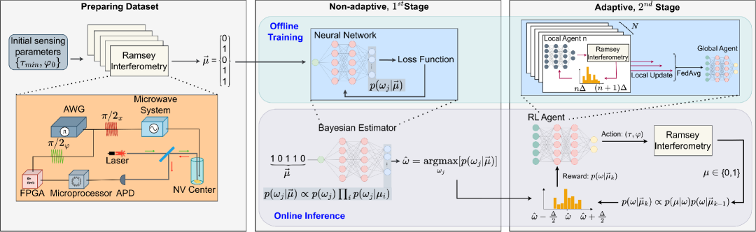
Figure 1: Framework of the proposed two-stage optimization method. The protocol consists of an offline training phase and an online inference phase. Prior to execution, two neural networks must be trained offline: one for the BNN estimator and another for the federated RL agent. To train the neural network for the BNN estimator, a large dataset is constructed using measurement outcomes from Ramsey experiments. These experiments are performed using a quantum sensor based on a single NV-center electron spin system. Each training sample is encoded as a one-hot vector representing a sequence of measurement outcomes $\vec{\mu}$, with the corresponding label being the posterior probability distribution $p(\omega_{j}\mid\vec{\mu})$. Here, $\omega_{j}$ denotes a discretized value from the magnetic field range $(0,\omega_{\text{max}})$. The neural network is trained to minimize a cross-entropy loss, effectively performing Bayesian inversion. For the training of the federated RL agent, the total magnetic field range is partitioned into $N$ equal-width intervals. Each interval $(n\Delta,(n+1)\Delta)$, with $\Delta=\omega_{\text{max}}/N$, defines a local environment for the $n$-th local RL agent. A dedicated RL agent is trained within each local environment, where the input after the $k$-th Ramsey experiment is the posterior distribution $p(\omega\mid\vec{\mu}^{(k)})$, approximated using a particle filter. The agent outputs an action $(\tau,\varphi)$, representing the sensing time and control phase for the next experiment. Upon receiving a measurement outcome $\mu$, the posterior distribution is updated using Bayes’ rule. Ramsey experiment is repeated until the predefined time resources are exhausted. Each local RL agent maximizes its cumulative reward and computes a local network parameter update. The global RL agent is then updated by aggregating all local updates using the FedAvg algorithm. Once offline training is completed, the protocol proceeds to the online inference phase. In the non-adaptive 1^st Stage, Ramsey experiments are performed using fixed sensing parameters $\tau_{\text{min}}={\pi}/{\omega_{\text{max}}}$ and $\varphi_{0}=0$ to generate a sequence of measurement outcomes $\vec{\mu}$. This sequence is input into the trained BNN estimator to produce an initial estimate $\hat{\omega}$, which narrows the magnetic field range to a subrange $\left(\hat{\omega}-\frac{\Delta}{2},\hat{\omega}+\frac{\Delta}{2}\right)$. In the adaptive 2^nd Stage, the trained global RL agent uses the posterior within this subrange to determine optimized sensing designs $(\tau,\varphi)$, thereby improving the estimation accuracy through adaptive Ramsey experiments.

The proposed protocol is poised to efficiently derive the optimal sensing time and control phase of an NV-center electron spin for single-shot Ramsey measurement. Suppose that the two basis states of a spin are $\ket{1}$ and $\ket{0}$. Ramsey measurement begins with a $\frac{\pi}{2}$ pulse, preparing the NV center in a superposition state $\frac{1}{\sqrt{2}}\left(\ket{0}+\ket{1}\right)$. The Zeeman shift, defined as $\omega:=\gamma B$, where $\gamma$ is the gyromagnetic ratio and $B$ is the D.C. magnetic field strength, then drives the evolution of the system. After a sensing time $\tau$, the state evolves to $\frac{1}{\sqrt{2}}\left(\ket{0}+e^{i\theta}\ket{1}\right)$, where $\theta=\omega\tau$ is the accumulated phase. Next, using a second $\frac{\pi}{2}$ pulse, the state is converted back to a measurable state $\frac{1}{2}(1+e^{i\theta})\ket{0}+\frac{1}{2}(1-e^{i\theta})\ket{1}$. Finally, the spin is read out in an appropriate basis to extract the phase $\theta$. The probability of obtaining outcome $0$ is given by

$$p(0\mid\omega)=\frac{1}{2}+\frac{1}{2}e^{-\tau/T_{2}}\cos(\omega\tau+\varphi),$$ (1)

and $p(1\mid\omega)=1-p(0\mid\omega)$. $\varphi$ is the control phase applied during the final $\frac{\pi}{2}$ pulse and $T_{2}$ represents the spin coherence time. The outcome of the measurement $m_{s}=0$ or $m_{s}=1$ is probabilistic and follows a periodic function weighted by a decay coefficient related to spin decoherence. To estimate the SoI $\omega$, one has to repeat Ramsey measurements for many rounds with possibly different configurations of $\{\tau,\varphi\}$, and then analyze the outcome statistics for inference. The research problem is now boiled down to two intertwined tasks, with one being the optimization of sensing parameters $\{\tau,\varphi\}$ and the other being the parameter estimation of $\omega$. In this work, we use estimation accuracy as the performance metric, captured by the mean square error (MSE) that is defined as $\text{MSE}(\hat{\omega},\omega):=|\hat{\omega}-\omega|^{2}$. Here, $\hat{\omega}$ is the estimated value, while $\omega$ (or equivalently $B$) is the true value of the D.C. magnetic field.

The existing literature has presented several solutions to this research problem, particularly in the context of quantum magnetic sensing [12, 26, 27]. Before reporting the results of this work, we first present three protocols whose underlying algorithm ideas reflect the mainstream that are broadly adopted in the community. The first one is the adaptive approach, commonly implemented as a closed loop that feeds back loss/reward for iterative update of control parameters. This is exemplified by the work by Bonato et al. [12]. They utilized the particle swarm optimization method that updated $\varphi$ by a fixed step size per iteration while selecting $\tau$ from a predetermined set. The stopping criteria of their algorithm was dictated by a closed-form equation borrowed from an established knowledge in [33]. Another algorithm bearing the similar adaptive nature is the use of RL, exemplified by Belliardo et al. in [27] (and an earlier work by Fiderer et al. [26] in a general quantum metrology context). Specifically, Belliardo et al. utilized a vanilla RL network to optimize both the sensing time $\tau$ and the controlled phase $\varphi$ [27]. This algorithm follows a black-box model, and its convergence depends on the loss function and the convergence threshold. In addition to the adaptive approach, another notable line of method is from the work by Nolan et al. [22] (though it is not directly applied to quantum magnetic sensing), coined as “NN-shots” protocol. It belongs to a non-adaptive approach in which a BNN is trained to perform parameter estimation, with the sensing time fixed at $\tau=\pi/\omega_{\text{max}}$. Compared with the conventional Bayesian updates that typically require an impractically large amount of observation data, the BNN in [22] can be trained using individual measurement outcomes without relying on an explicit physical model or fitting function. This model-agnostic feature makes the BNN particularly well suited for estimation tasks in scenarios involving finite detection resolution and noisy probe states. In this work, we will use the works by Bonato et al. [12], Belliardo et al. in [27], and NN-shots by Nolan et al. [22], representing different levels of algorithmic adaptiveness, as the baselines for performance comparison.

An overview of this work’s protocol is shown in Fig. 1. In summary, it is based on a two-stage progressive optimization method. Each stage consists of an offline training phase and an online inference phase, as shown on the green panel and gray panel, respectively, in Fig. 1. For presentation clarity, we focus on illustrating the runtime procedure of this protocol while directing the readers to Appendix A-B for the details of dataset preparation and model training. To begin with, we run a certain number of Ramsey measurements using the same setup of $\tau_{\text{{min}}}=\pi/\omega_{\text{max}}$ and $\varphi_{0}\ =0$. This is because the measurement outcome in Eq. (1) is a periodic signal, to avoid ambiguity, $\omega\tau+\varphi\leq\pi$ must hold. Therefore, for an unknown magnetic field in a wide range, we initiate the sensing time in such a conservative but non-optimal way. After collecting all the measurement results $\vec{\mu}$, the trained BNN estimator in the 1^st Stage is employed to estimate the SoI $\omega$. The output of the BNN estimator offers two fold of information — the estimated value $\hat{\omega}$ and its associated uncertainty level $\Delta$. This output is subsequently used as the initial input of the protocol’s 2^nd Stage. Compared with the 1^st Stage, the model in the 2^nd Stage is adaptive and aims to optimize the sensing parameters $(\tau,\varphi)$ over a small number of iterations. Specifically, based on $(\hat{\omega},\Delta)$ from the 1^st Stage, we construct an ensemble of $\omega$’s in the range of $\left(\hat{\omega}-\frac{\Delta}{2},\hat{\omega}+\frac{\Delta}{2}\right)$ because with a high confidence level we believe the true value lies within this range. Then, we use the particle filter method to assign each $\omega$’s with a weight, which is initialized by the posterior probability from the 1^st Stage. After the global RL agent jump starts, it creates an action comprising a new tuple of $(\tau,\varphi)$. We perform a new Ramsey measurement based on this setup and collect the measurement result $\mu$ to update the posterior distribution. This closed-loop iteration continues till the total sensing time budget exhausts or the RL agent’s loss function diminishes below a threshold. When the 2^nd Stage completes, we shall be able to refine $\hat{\omega}$ (the estimation from the 1^st Stage) to approach the true value.

To evaluate the performance of the proposed method, we use the same experiment platform as in [12]. While the readers can refer to [12] for full experiment details, a few notable information is listed below. The platform is a single spin system in a NV center with single-shot readout capability. The spin coherence time is $96\mu$s. Every Ramsey measurement comes with a sensing time $\tau$ and a system overhead of $240\mu$s which accounts for state preparation and readout overhead. The magnetic sensing task has a total time budget of $R_{\text{max}}=22{,}000~\mu$s, which meets the real-time constraints of many applications such as geo-localization and medical diagnosis. The results presented in later sections follow the windowing approach in [27]. This is to smooth out the variability in time consumption across individual Ramsey measurements. Specifically, the estimation values (or MSE) within a fixed time window of $500\,\mu\text{s}$ (or, the estimation for roughly 2-3 measurement outcomes) are averaged to yield a single representative point. The final partial window is excluded if it is less than $500~\mu$s.

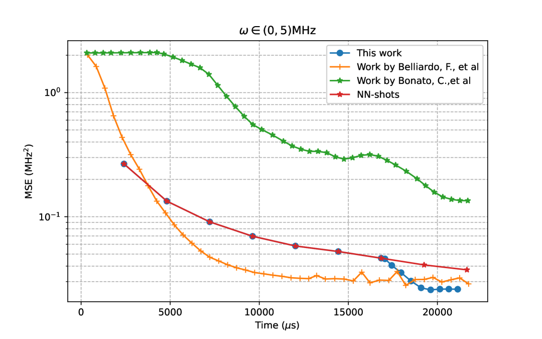
(a)

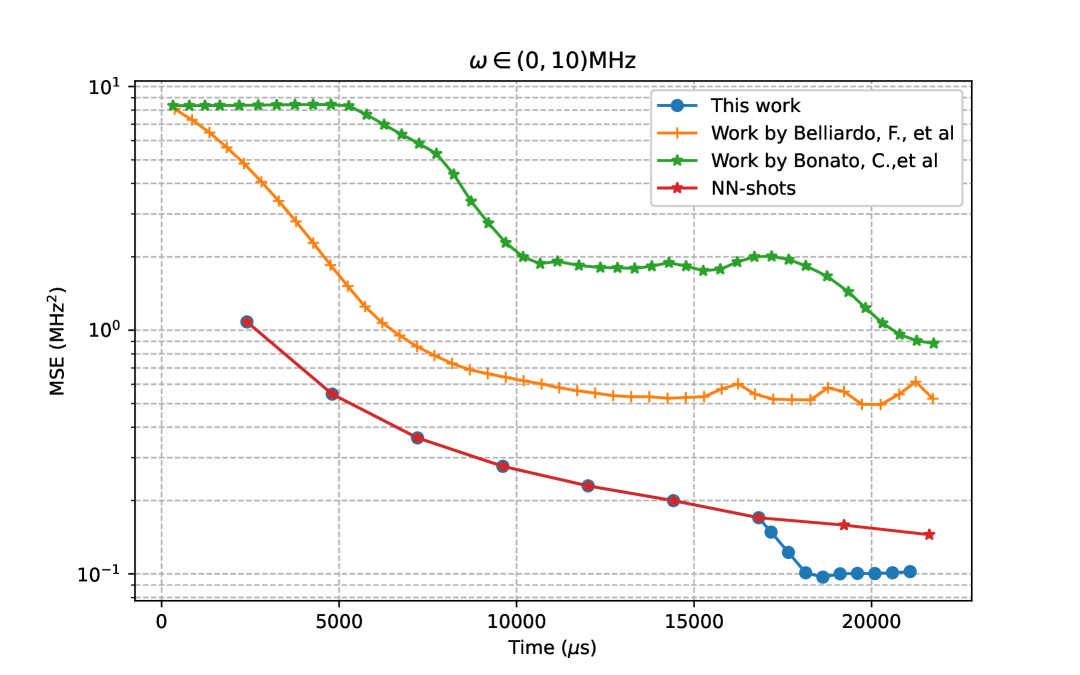
(b)

Figure 2: Comparison of estimation performance across different methods. (a) shows the performance under the magnetic field range $\omega\in(0,5)$ MHz. (b) illustrates the performance under the range $\omega\in(0,10)$ MHz. In all cases, the non-adaptive 1^st Stage consists of 70 measurement shots. The total available time resources are limited to $22,000~\mu$s, with a per-shot overhead of $240~\mu$s for spin initialization and readout, following Ref. [12]. The curves for the protocols proposed by Belliardo et al. [27] and Bonato et al. [12] begin after the first measurement shot, while the curves for NN-shots [34] and the protocol proposed in this work begin after the initial 10 measurement shots.

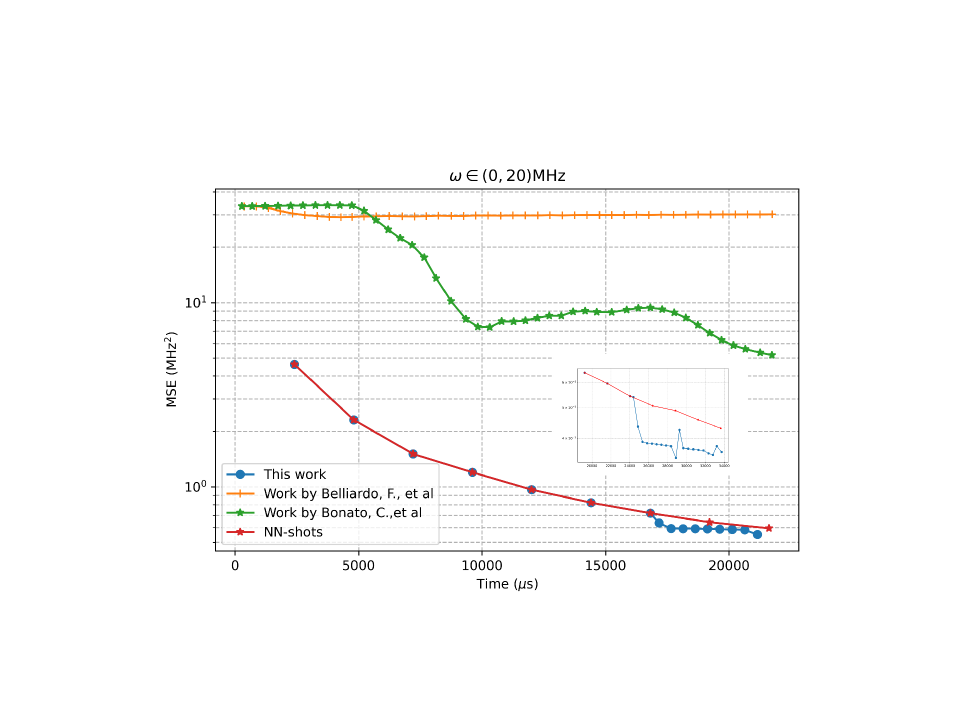
Figure 3: Comparison of estimation performance under a wide magnetic field range $\omega\in(0,20)$ MHz. The non-adaptive 1^st Stage consists of 70 measurement shots. The inset figure is a zoom-in view of the performance of the proposed protocol compared with that of the NN-shots method in [34] when the number of measurement shots in the non-adaptive 1^st Stage is increased to 100.

Fig. 2 presents the performance of various sensing protocols under two magnetic field ranges: $\omega\in(0,5)$ MHz and $\omega\in(0,10)$ MHz. The results demonstrate that the proposed protocol in this work outperforms existing methods in terms of estimation accuracy under limited time resources. In Fig. 2(a), under the magnetic field range of $\omega\in(0,5)$ MHz, the proposed method outperforms the NN-shots approach of Nolan et al. [34] by $30.2\%$, and the method of Belliardo et al. [27] by $9.5\%$. The method by Belliardo et al. also shows a $22.9\%$ improvement over the NN-shots approach. In Fig. 2(b), within the broader field range of $\omega\in(0,10)$ MHz, the proposed method achieves a $29.5\%$ performance improvement over the NN-shots method. In Fig. 2(a) where $\omega$ is in a narrower range, the RL-based method by Belliardo et al. [27] shows better performance than the methods by Bonato et al. [12] and Nolan et al. [34]. This is attributed to the adaptive nature of RL that optimizes $\{\tau,\varphi\}$ collectively; while the other two methods are either non-adaptive [34] or have smaller optimization space [12]. Interestingly, when the range of $\omega$ broadens, Fig. 2(b) shows that although the RL-based method by Belliardo et al. [27] is still better than the method by Bonato et al. [12], it underperforms the NN-shots method by Nolan et al. [34]. This suggests that the RL agent trained in [27] lacks the capability required for effective optimization across a much wider solution space (i.e., a wider field range). In brief summary, the lessons learned from these existing methods are two-fold: (1) the vanilla BNN estimator using non-adaptive parameter setup is ideal for estimating $\omega$ in a wide range; (2) the RL method is well-suited to optimize sensing parameters in a small search space but fails to generalize when the space explodes. To combine the benefits of the two methods, this work’s approach includes running the BNN estimator with fixed parameter setup for one-shot estimation and further utilizing a federated RL agent to further optimize the parameters within a subrange of $\omega$. As shown in Fig. 2(a-b), our method manages to boost the performance beyond the best among the state of the art.

Fig. 3 further shows the performance of same baseline protocols and ours in an extended magnetic field range of $\omega\in(0,20)$ MHz. The results indicate that our method achieves superior estimation accuracy compared to others, given the same limited time resources ($R_{\text{max}}=22{,}000~\mu$s). The proposed method demonstrates a $7.5\%$ performance improvement over the NN-shots method of Nolan et al. [34]. Furthermore, when the number of measurement shots in the 1^st Stage is increased to 100, the inset figure demonstrates that the advantage becomes more pronounced, with the proposed method outperforming the NN-shots approach [34] by $17.6\%$. These results confirm that the RL agent in the 2^nd Stage of our protocol is capable of optimizing sensing parameters to enhance estimation accuracy and efficiency. In addition, it is observed that the estimation accuracy of the protocol by Bonato et al. [12] exceeds that of Belliardo et al. [27] in this large field range. Recall that the method in [12] employs a partially adaptive strategy — only phase $\varphi$ is adaptively optimized while $\tau$ is selected from a predetermined set. The method in [27] optimizes both $\varphi$ and sensing time $\tau$. Fig. 3 reveals that the latter method does not give any edge. This comparison highlights the potential advantage of fixing sensing time $\tau$ (ideally equal to $\tau_{\text{min}}$) in the early stage of the protocol to save the RL agent from iterating over unnecessarily long steps for the search of an optimal parameter setup. This design principle is particularly helpful when the total sensing time as a resource is limited and meanwhile the range of the magnetic field is large.

Moreover, we understand that the convergence rate and optimality in the vanilla RL framework is cursed by large search space. To enhance its performance for wide-range magnetic field sensing, we introduce federated learning into the training process of the RL agent used in the 2^nd Stage. As shown in the offline training phase for the 2^nd Stage in Fig. 1, the entire magnetic field range is partitioned into multiple intervals. Each interval is treated as a local environment, corresponding to a specific subrange of the D.C. magnetic field. A dedicated local RL agent is trained within each of these environments, producing local updates to the neural network parameters. These local updates are then aggregated using the FedAvg algorithm to update a global RL agent. Importantly, the local environments remain fixed throughout the training process, ensuring that each local agent learns to optimize sensing parameters for the $\omega$ within its designated subrange. The posterior probability distribution, i.e., the Bayesian update of the estimated D.C. magnetic field, is used as the input to the global RL agent. This distribution is approximated using a particle filter implemented via a sequential Monte Carlo (SMC) algorithm. During the online inference phase, the range of the particles is set to the subrange of $\omega$ identified based on the estimation value $\hat{\omega}$ and associated uncertainty $\Delta$ obtained from the 1^st Stage. This innovation, which we call federated RL agent, plays a vital role for the outperforming results of our protocol shown in the earlier figures.

Federated-RL

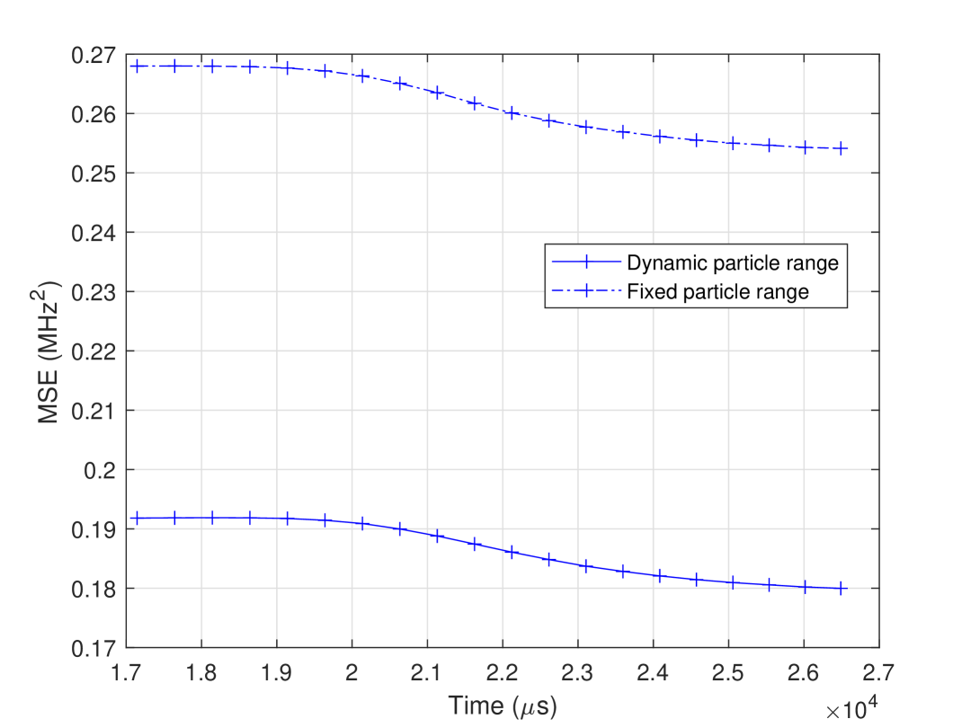
oneM-RL

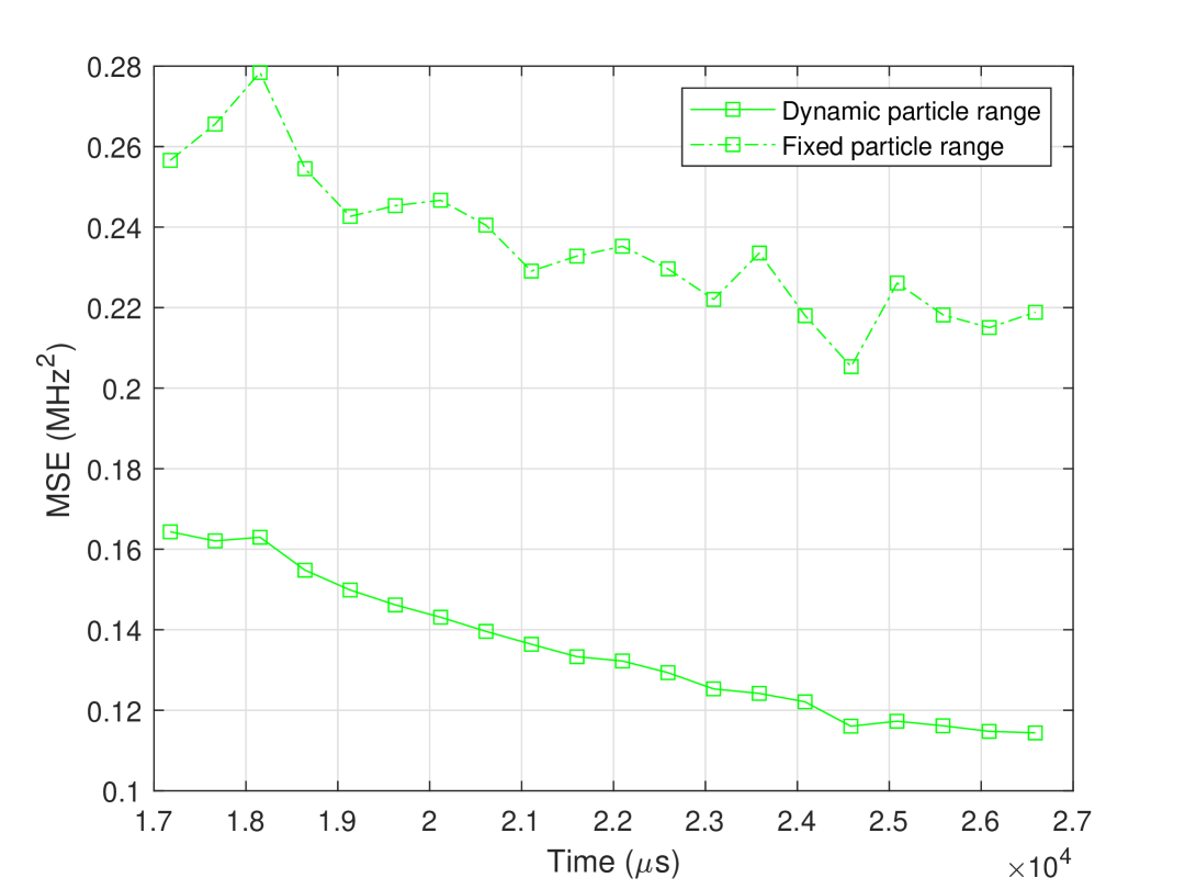
multipleM-RL

Figure 4: Comparison of different strategies for setting the particle range. oneM-RL stands for one single RL Model while multipleM-RL represents many parallel RL Models. The results are collected for $\omega\in(0,10)$MHz.

To further highlight the advantages of the federated RL agent, we compare its standalone performance with two additional RL training strategies in the following experiments. The results are shown in Fig. 4 and Fig. 5. Here, Federated-RL refers to the proposed method used in this work, in which a global RL agent is trained via the FedAvg algorithm by aggregating updates from multiple local agents, each trained within a specific subrange of the magnetic field. oneM-RL denotes a sequential training approach, where a single RL agent is trained across all local environments one after another. multipleM-RL represents a scheme in which multiple RL agents are independently trained within their respective local environments, without any aggregation or parameter sharing. This comparison aims to demonstrate that our proposed method not only achieves superior generalization across the wide magnetic field range but also maintains the efficiency and adaptability needed for high-accuracy estimation. Note that the notion of generalization considered in this work differs slightly from that typically discussed in the context of federated learning. Here, generalization refers to the ability of the global RL agent to outperform individual local agents across the entire estimation range. While each local RL agent is trained to identify an optimal experimental design within its assigned subrange, the global RL agent integrates information from all subranges and is thus capable of learning a more general policy that performs well across the full estimation domain. The evaluation of the three methods is based on two setups, one being the dynamic particle range that is defined around the estimation value obtained from the 1^st Stage whereas another being the fixed particle range corresponding to one of the predefined intervals used during the training process. The results in Fig. 4 show that, among all three models, the dynamic particle range setup consistently yields better performance than the fixed particle range setup. This improvement is attributed to the fact that the true value of the D.C. magnetic field is more likely to be found near the estimated value of the 1^st Stage. More importantly, this work’s Federated-RL framework outperforms the other two RL frameworks in terms of MSE, almost for any given sensing time budget in the x-axis. The results in Fig. 4 justify the choice of Federated-RL framework in this work.

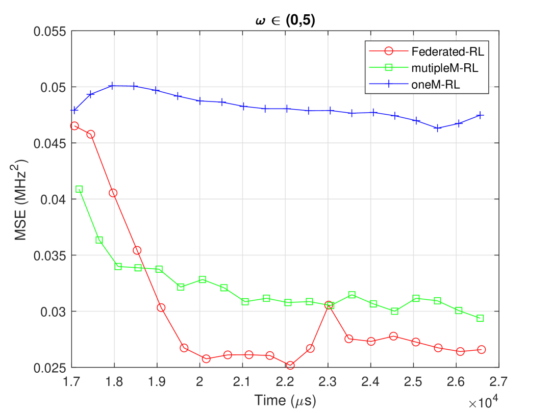
(a)

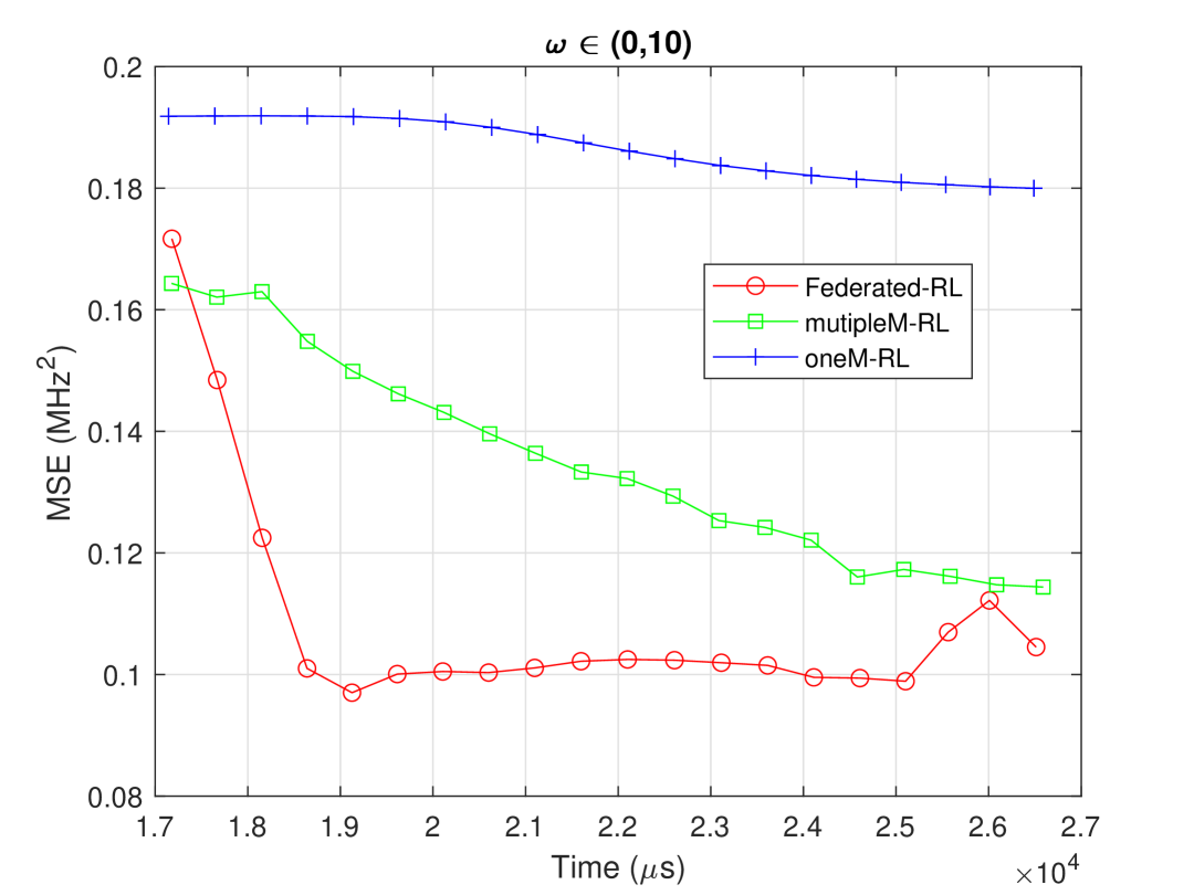
(b)

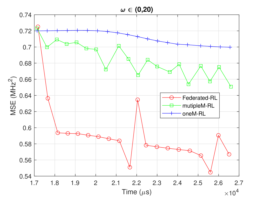
(c)

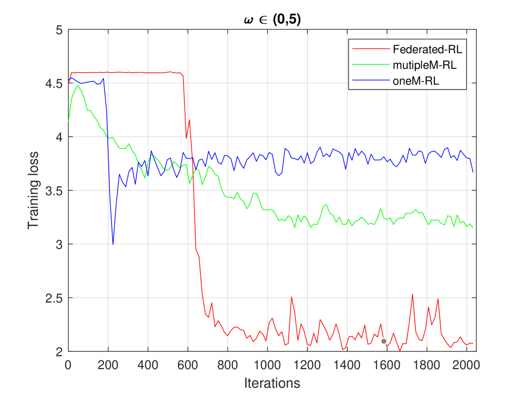
(d)

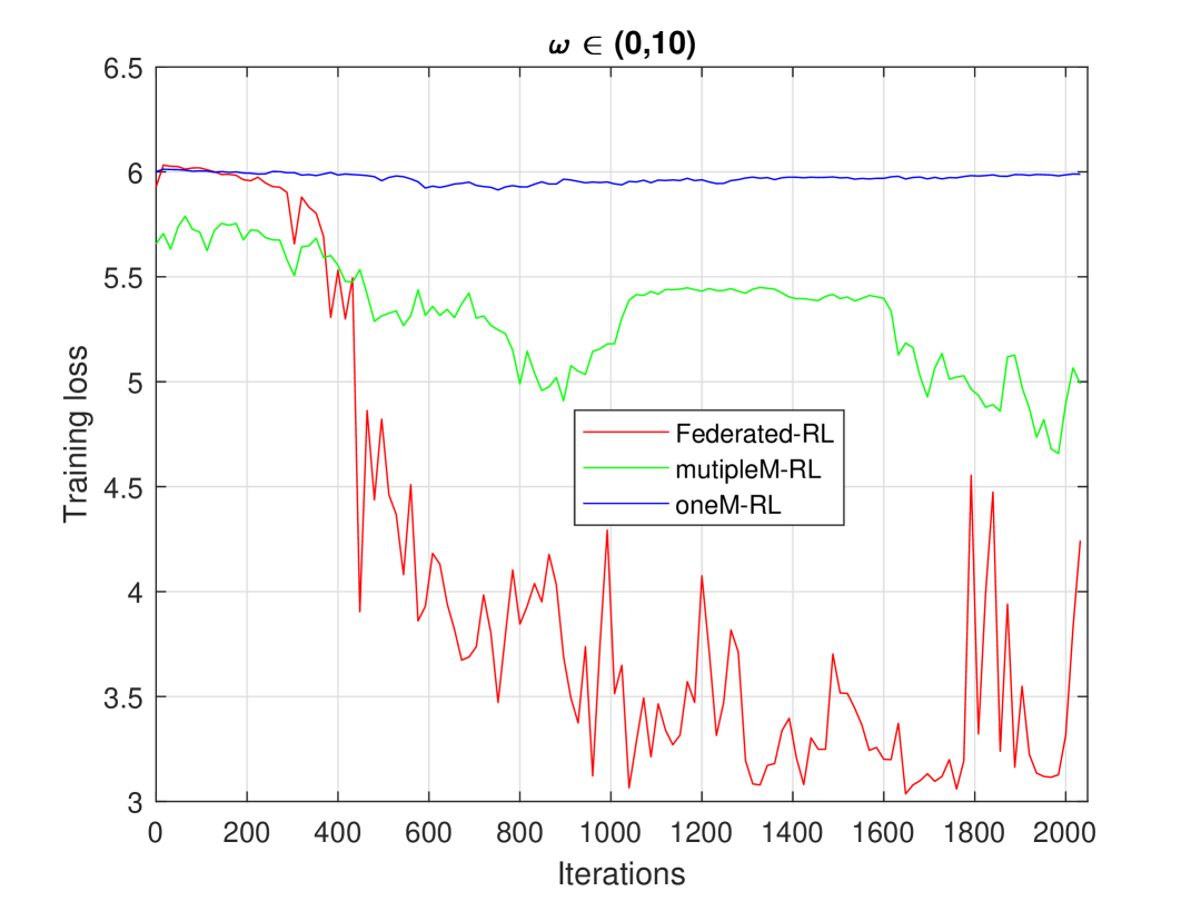
(e)

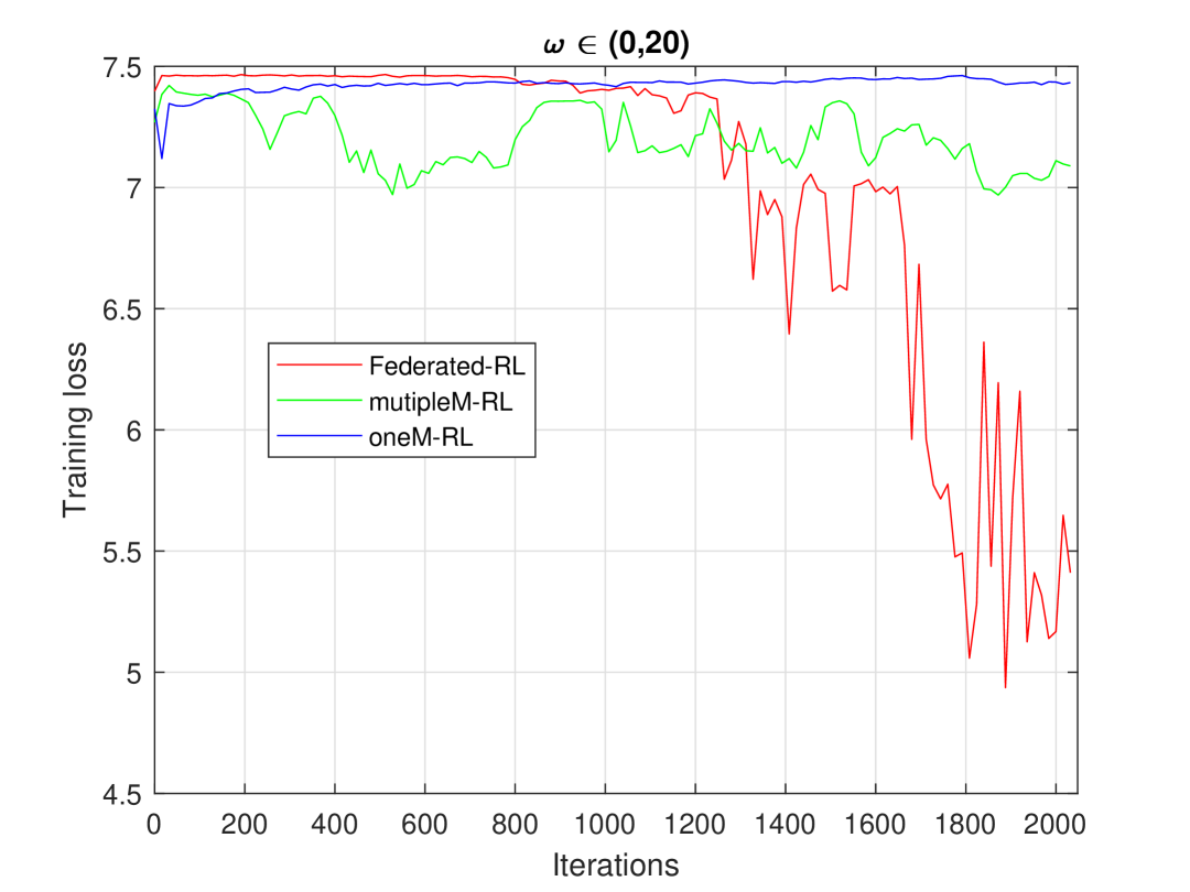
(f)

Figure 5: Comparison of performance among the three RL agents with the dynamic particle range. (a)–(c) show the estimation accuracy of the 2^nd Stage following 70 measurement shots in the 1^st Stage; and (d)-(f) compare their convergence rate and training loss.

Next, Fig. 5 compares the performance of the three RL agents under different magnetic field ranges: $\omega\in(0,5)$ MHz, $\omega\in(0,10)$ MHz, and $\omega\in(0,20)$ MHz. The results demonstrate that the proposed federated RL agent consistently achieves significantly higher estimation accuracy and efficiency across all tested field ranges. This performance advantage is consistent with the training loss curves shown in Fig. 5(d)–(f), confirming that our approach achieves much lower training loss while maintaining a similar level of convergence speed. In Supplementary Results of Appendix C, we further demonstrate the real-time evolution of sensing parameters as the adaptive 2^nd Stage proceeds. This result will offer a granular view of the trajectory of sensing parameter evolvement, elucidating the reason why our protocol achieves superior performance over the methods by Belliardo et al. [27] and Bonato et al. [12].

3 Methods

The framework of the proposed two-stage optimization method is illustrated in Fig. 1. In the non-adaptive 1^st Stage, a BNN estimator is employed to narrow the range of the estimated magnetic field. The BNN takes the measurement outcomes from a sequence of Ramsey experiments as input and outputs an estimated magnetic field value. To avoid ambiguity arising from the periodic nature of the Ramsey signal, the sensing time is fixed at $\tau_{\text{min}}=\pi/\omega_{\text{max}}$ and the control phase $\varphi_{0}=0$. Details of the BNN training process are provided in Supplementary Methods I.

In the adaptive 2^nd Stage, an RL agent is employed to optimize the sensing time and control phase for estimating the magnetic field within a subrange centered around the value obtained from the 1^st Stage. This subrange is defined as an interval with a width slightly greater than twice the estimated error. While a narrower range reduces the RL agent’s learning complexity, it raises the concern that the true value of the magnetic field may fall off the range. To balance the learning complexity and estimation accuracy, federated learning is employed during the offline training of the RL agent, enabling it to generalize effectively across all possible subranges. The details of the federated RL agent training process are provided in Supplementary Methods II. Specifically, a key input to the federated RL agent is the posterior distribution of the estimated magnetic field, which is approximated using a particle filter. The posterior distribution $p(\omega\mid\vec{\mu}^{(k)})$ is represented using a particle filter consisting of $P$ weighted particles $\{\omega_{p}\}_{p=1}^{P}$, uniformly distributed over a specified subrange of the magnetic field. During the online inference phase, particles are sampled within the interval $\left(\hat{\omega}-\frac{\Delta}{2},\hat{\omega}+\frac{\Delta}{2}\right)$, where $\hat{\omega}$ denotes the estimation value obtained from the 1^st Stage. In the offline training phase, each local RL agent corresponds to a fixed subrange $\left(n\Delta,(n+1)\Delta\right)$, where $\Delta={\omega_{\text{max}}}/{N}$ and $N$ is the total number of RL agents. Initially, all particles $\omega_{p}$’s are assigned uniform weights $a_{p}={1}/{P}$. The posterior distribution $p(\omega\mid\vec{\mu}^{(k)})$ is approximated as a discrete sum of a $\delta$-function:

$$p(\omega\mid\vec{\mu}^{(k)})=\sum_{p=1}^{P}a_{p}^{k}\cdot\delta(\omega-\omega_{p}),$$ (2)

where $\vec{\mu}^{(k)}$ denotes the sequence of measurement outcomes up to the $k$-th Ramsey experiment. According to Bayes’ theorem, the posterior is recursively updated via

$$p(\omega\mid\vec{\mu}^{(k)})\propto p(\mu\mid\omega)\cdot p(\omega\mid\vec{\mu}^{(k-1)}),$$ (3)

where $\mu$ is the latest measurement outcome. Accordingly, the weight of the $p$-th particle is updated as

$$a_{p}^{k}=a_{p}^{k-1}\cdot p(\mu\mid\omega_{p}).$$ (4)

During the adaptive 2^nd Stage, each iteration consists of three steps. First, the last round of Ramsey measurement produces a measurement outcome $\mu$ that results in the update of posterior probability in Eq. (3) and its associated particle weight in Eq. (4). Then, the posterior probability is approximated by the particle filter method following Eq. (2). It is further combined with the remaining time resources as the input to the federated RL agent, which then outputs an optimized sensing time and controlled phase for the next Ramsey measurement. Second, a Ramsey experiment is performed using these optimized sensing parameters to obtain a new measurement outcome. Third, the posterior distribution is updated again according to Bayes’ rule in Eq. (3), and each particle is reweighted based on the likelihood of the new measurement result as in Eq. (4). This process is repeated until the total available time resources are exhausted.

4 Discussion

Several key directions about the proposed two-stage optimization method warrant further investigation to enhance its practical performance and applicability.

1. Analysis of $\Delta$: The choice of $\Delta$ should take into account the estimation error introduced during the adaptive stage. This error arises from a combination of factors, including the training error, the size of the measurement vector $\vec{\mu}$, the dimensionality of the BNN’s output layer (reflecting the granularity of the discretization of $\omega$), the posterior approximation error, and others. From existing knowledge [35], we understand that in an ideal situation where the BNN estimator is sufficiently well-trained, the output Bayesian posterior probability shall asymptotically converges to the Gaussian distribution as the number of measurements $M$ in $\vec{\mu}$ increases:

$$p(\omega_{j}|\vec{\mu})\approx\sqrt{\frac{MF(\omega)}{2\pi}}\,e^{-\frac{MF(\omega)}{2}(\omega_{j}-\omega)^{2}}$$ (5)

The distribution is centered at the true value $\omega$ and with variance $1/[MF(\omega)]$ where $F(\omega)$ is the Fisher information. However, selecting the confidence level $\Delta$ based on the standard deviation from Eq. (5) may not be very trustworthy in a practical setting. Therefore, in this work, $\Delta$ is empirically fixed as $\omega_{\text{max}}/N$, where $N$ is the number of local RL agents in the adaptive stage. To ensure that the adaptive stage operates within a reliably estimated subrange, the BNN must constrain its estimation error $|\hat{\omega}-\omega|$ below ${\Delta}/{2}$. Provided that the BNN estimator exhibits diminishing returns in accuracy for increasingly narrow estimation ranges due to its fixed approximation capacity, the error needs only to be marginally smaller than ${\Delta}/{2}$. For instance, under magnetic field ranges $\omega\in(0,5),(0,10),(0,20)$ MHz with $\Delta=0.5,1,2$ MHz respectively, we observe that the corresponding BNN’s estimation errors after 70 Ramsey measurements are approximately $0.22,0.41,0.85$ MHz. While the chosen $\Delta$ performs well within the protocol setting of this work, we acknowledge that it can be further reduced or dynamically adjusted at runtime without increasing the complexity of the BNN model or the number of measurement samples (which otherwise results in waste of time resources). Such optimization has the potential to further enhance the overall estimation accuracy.

2. Time Resource Allocation: A practical quantum sensing system may operate under limited time budget due to the latency requirement of a sensing task or the system overhead. In this work, we follow the experimental setup in Bonato et al. [12] and set the time budget be $R_{\text{max}}=22{,}000~\mu$s. We spare 70 measurement shots to the 1^st Stage while allocating the rest to the 2^nd Stage. In this configuration, we in fact allocate $\left(t_{\text{inactive}}+{\pi}/{\omega_{\text{max}}}\right)\times 70\mu$s time resources to the 1^st Stage when accounting for the inactive time $t_{\text{inactive}}$ spent for preparing, reading out, and resetting qubit for each shot of measurement. Following the setup in [12], we let $t_{\text{inactive}}$ be 240 $\mu$s. In an ideal situation that time resource is not a constraint, by accommodating 100 measurement shots in the 1^st Stage while keeping the same time for the 2^nd Stage, the inset figure in Fig. 3 reveals that the accuracy can be further boosted by 10%. However, in a realistic time-limited context, the resource allocation between the two inference stages must be carefully planned. We believe that further analysis of $\Delta$ mentioned in the prior section and exploration of the parallelism of the two stages will shed the light on the pathway for time resource optimization, leading to further improvement on estimation accuracy.

3. Scalability Beyond NV Centers: While our protocol is demonstrated using a single NV center in a diamond as the quantum sensor platform, the optimization framework is inherently sensor-agnostic. The BNN estimator only requires training data comprising measurement outcomes and does not depend on sensor-specific physics. Similarly, the RL agent is trained to optimize sensing parameters (e.g., time, phase) and can be adapted to other sensor platforms by redefining the action space. For example, the protocol can be extended to systems beyond the single-shot readout capability by treating the Bayesian update input as a vector $\vec{\mu}$ of aggregated outcomes. This flexibility enhances its applicability to a broad class of quantum sensing and metrology systems.

4. Robustness to Noise: A significant advantage of the proposed method is the separation of offline training and online inference. Both the BNN estimator and the RL agent can be trained on large, noisy datasets, allowing them to learn noise-robust representations and policies. Furthermore, federated learning enables the RL agent to aggregate updates from local environments with varied noise characteristics, resulting in a globally trained agent with improved generalization to practical sensing scenarios. For instance, if considering the measurement noises, we can update Eq. (1) with $p(0\mid\omega)=\frac{1+F_{0}-F_{1}}{2}+\frac{F_{0}+F_{1}-1}{2}e^{-\tau/T_{2}}\cos(\omega\tau+\varphi)$ where $F_{0}$ and $F_{1}$ are readout fidelity for 0s and 1s respectively. By profiling the noise models of a quantum sensing system at design time, the inference framework can be adjusted offline without introducing any runtime overhead. This flexibility offers great robustness to noisy intermediate-scale quantum (NISQ) devices.

In summary, the proposed two-stage optimization method offers a scalable, efficient, and noise-robust solution for various quantum sensing apparatus. Future work will explore optimal time allocation strategies, adaptive tuning of $\Delta$, and applications to other sensor platforms, further enhancing its utility for precision metrology in diverse experimental settings.

5 Conclusion

In this work, we presented a new quantum magnetic sensing protocol for a NV center system with only single-shot readout capability. The protocol introduces a novel progressive optimization strategy that led to a superior performance over the state-of-the-art methods, most notably a 7.5% accuracy improvement for estimating a wide-range magnetic field within a constrained sensing time budget of less than 22 ms. Furthermore, our analysis showed that the protocol’s framework is both scalable to other quantum sensing platforms and robust against various noise sources.

Supplementary information Not applicable.

Acknowledgments J. Liu discloses support for the research of this work from National Science Foundation [grant number 2304118 and 2326746].

Declarations

• Data availability: The datasets generated during and/or analysed during the current study are available from the corresponding author on reasonable request.

• Code availability: The underlying code for this study is not publicly available but may be made available to qualified researchers on reasonable request from the corresponding author.

Appendix A Supplementary Methods I

Training of the BNN Estimator

The BNN estimator is implemented as a fully connected feed-forward neural network comprising two hidden layers, each with 32 neurons. The hidden layers employ the ReLU activation function, defined as $\max(x,0)$. The input and output dimensions of the network are 1 and 100, respectively. We encode one training sample (or measurement outcome) from the dataset $\mathcal{D}_{\omega}$ as a one-hot vector and feed into the input layer of BNN. The output layer is normalized using the softmax function to produce a valid probability distribution over discrete magnetic field values. Specifically, the network outputs a posterior distribution $p(\omega_{j}\mid\mu_{i})$, which represents the probability of the magnetic field taking the value $\omega_{j}$ conditioned on a single-shot measurement outcome $\mu_{i}$.

The loss function is defined as the average negative log-likelihood across all training samples:

$$\mathcal{L}=-\frac{1}{b_{\omega}|\mathcal{D}_{\omega}|}\sum_{\ell=1}^{b_{\omega}}\sum_{i=1}^{|\mathcal{D}_{\omega}|}\log p(\omega_{\ell}\mid\mu_{i,\ell}),$$ (6)

where $b_{\omega}$ denotes the number of discrete values within the range $\omega_{\ell}\in(0,\omega_{\text{max}})$, and $|\mathcal{D}_{\omega}|$ is the number of measurement outcomes in the dataset. To improve generalization and training stability, an $L_{2}$ regularization term is added to the loss. Optimization is performed using the Adam algorithm [36] for stochastic gradient descent. All neural network estimators are implemented and trained using the JAX framework [37].

Assuming conditional independence of measurements and a uniform prior over $\omega$, the posterior distribution over $\omega_{j}$ given a sequence of $M$ measurement outcomes $\vec{\mu}^{(M)}=\{\mu_{1},\mu_{2},\dots,\mu_{M}\}$ is given by the normalized product of individual posteriors:

$$p(\omega_{j}\mid\vec{\mu})\propto\prod_{m=1}^{M}p(\omega_{j}\mid\mu_{m}).$$ (7)

Equation (7) can be obtained via Bayesian updating. Specifically, the posterior distribution after incorporating the $M$-th measurement outcome $\mu_{m}$ is given by

$$p(\omega_{j}\mid\vec{\mu}^{(M)})=p(\mu_{m}\mid\omega_{j})\cdot p(\omega_{j}\mid\vec{\mu}^{(M-1)}),$$ (8)

where, according to Bayes’ theorem, the conditional probability $p(\mu_{m}\mid\omega_{j})$ can be expressed as

$$p(\mu_{m}\mid\omega_{j})=\frac{p(\omega_{j}\mid\mu_{m})\cdot p(\mu_{m})}{p(\omega_{j})}.$$ (9)

Substituting into the update rule yields

$$p(\omega_{j}\mid\vec{\mu}^{(M)})=\frac{p(\omega_{j}\mid\mu_{m})\cdot p(\mu_{m})}{p(\omega_{j})}\cdot p(\omega_{j}\mid\vec{\mu}^{(M-1)}).$$ (10)

By iterating this update over successive measurements, one arrives at Eq. (7). Here, $p(\omega_{j})$ represents the prior distribution, and $p(\mu_{m})$ serves as a normalization factor to ensure the posterior remains properly normalized. Thus, the posterior distribution shown in Fig. 1 is given by

$$p(\omega_{j}\mid\vec{\mu}_{M})\propto p(\omega_{j})\cdot\prod_{m=1}^{M}p(\omega_{j}\mid\mu_{m}).$$ (11)

And the final estimation value is then obtained via maximum a posteriori (MAP) inference:

$$\hat{\omega}=\arg\max_{\omega_{j}}\left[p(\omega_{j}\mid\vec{\mu})\right].$$ (12)

A training dataset for the BNN estimator consists of measurement outcomes, i.e., classical bit-strings, denoted as $\mu_{m}\in\{0,1\}$. These outcomes are collected at $b_{\omega}$ distinct true parameter values uniformly sampled across the range $\left(0,\omega_{\text{max}}\right)$. For every Ramsey measurement, we always choose $\tau=\pi/\omega_{\text{max}}$ and $\varphi_{0}=0$ for quantum magnetic sensing. For each value of $\omega$, a sequence of $|\mathcal{D}_{\omega}|$ Ramsey measurements are performed and their outcomes are recorded. Thus, the total number of bit-strings in the training dataset is $b_{\omega}\times|\mathcal{D}_{\omega}|$, forming a two-dimensional binary array of shape $\left(b_{\omega},|\mathcal{D}_{\omega}|\right)$. The batch size is $b_{\omega}=100$ and the dataset comprises $|\mathcal{D}_{\omega}|=5,000$ samples. Training is performed over 8,000 iterations with a learning rate of $10^{-3}$.

Appendix B Supplementary Methods II

Training of the Federated Reinforcement Learning Agent

The RL agent is implemented as a fully connected neural network comprising 5 hidden layers, each with 64 neurons. The input and output dimensions of the network are 5 and 2, respectively. A hyperbolic tangent (tanh) activation function is applied to the final layer to bound the output within the interval $[-1,1]$.

The input (observation) to the agent after the $k^{\text{th}}$ Ramsey experiment is denoted as

$$s_{k}=\left(\widetilde{\omega}_{k},\widetilde{\sigma}_{k},\Gamma_{k},\widetilde{k},\widetilde{R}_{k}\right),$$ (13)

where all components are scaled to lie within the range $[-1,1]$. Here, $\widetilde{\omega}_{k}$ represents the normalized mean of the estimation posterior, and

$$\widetilde{\sigma}_{k}=-\frac{2}{10}\ln\sqrt{\Sigma_{k}}-1,$$ (14)

with $\Sigma_{k}$ denoting the covariance (or variance in the scalar case) around the posterior mean, defined as

$$\Sigma_{k}:=\int(\omega-\hat{\omega}_{k})(\omega-\hat{\omega}_{k})^{\top}p(\omega\mid\vec{\mu}^{(k)})\,d\omega,$$ (15)

The term $\Gamma_{k}$ represents the correlation matrix of the posterior distribution. For the single-parameter estimation problem considered here, this simplifies to $\Gamma_{k}=1$. The variables $\widetilde{k}$ and $\widetilde{R}_{k}$ denote the normalized experiment index and normalized consumed time resources, respectively.

The agent, parameterized by $\boldsymbol{\lambda}$, outputs two actions: sensing time $\tau$ and controlled phase $\varphi$. This new sensing setup is then applied to the subsequent Ramsey measurement to refine the parameter estimation.

The local loss function, capturing the cumulative estimation error over a sequence of experiments, serves as the reward signal for training [26]. For agent $n$ trained on dataset $\mathcal{D}_{n}$, the loss is defined as

$$\mathcal{L}_{n}(\boldsymbol{\lambda}):=\frac{1}{K|\mathcal{D}_{n}|}\sum_{k=1}^{K}\sum_{i=1}^{|\mathcal{D}_{n}|}\ell(\widehat{\omega}_{i,k},\omega_{i}),$$ (16)

where $K$ is the maximum number of Ramsey experiments under the limited time resource $R_{\text{max}}$, $\omega_{i}\in[n\Delta,(n+1)\Delta)$ denotes the true value and $\widehat{\omega}_{i,k}$ is the estimate after the $k^{\text{th}}$ Ramsey measurement. The estimate is computed as a weighted sum over basis points:

$$\widehat{\omega}_{i,k}=\sum_{p=1}^{P}a_{p}^{k}\cdot\widehat{\omega}_{i,k,p}\cdot\delta(\omega-\omega_{p}).$$ (17)

The global loss function is defined as the weighted average of all local losses:

$$\mathcal{L}(\boldsymbol{\lambda}):=\frac{1}{\sum_{n=1}^{N}|\mathcal{D}_{n}|}\sum_{n=1}^{N}|\mathcal{D}_{n}|\,\mathcal{L}_{n}(\boldsymbol{\lambda}).$$ (18)

The federated learning objective is to determine the optimal global parameters:

$$\boldsymbol{\lambda}^{*}=\arg\min_{\boldsymbol{\lambda}}\mathcal{L}(\boldsymbol{\lambda}).$$ (19)

During each training iteration $t$, local model parameters are updated using the Adam optimizer as

$$\boldsymbol{\lambda}_{n}^{t+1}=\boldsymbol{\lambda}_{n}^{t}-\eta\nabla\mathcal{L}_{n}(\boldsymbol{\lambda}_{n}^{t}),$$ (20)

where $\eta$ is the learning rate. The global parameters are then updated by aggregating the local updates:

$$\boldsymbol{\lambda}^{t+1}=\sum_{n=1}^{N}\frac{|\mathcal{D}_{n}|}{\sum_{n=1}^{N}|\mathcal{D}_{n}|}\boldsymbol{\lambda}_{n}^{t+1}.$$ (21)

The RL agent is trained over 2,048 iterations with a batch size of 1,024 and a learning rate of $\eta=10^{-3}$. The number of agents participating in the federated setting is set to 10. During training, the number of particles $P$ used to represent the posterior distribution is chosen according to the maximum frequency range: $P=240$ for $\omega_{\text{max}}=5~\mathrm{MHz}$ and $10~\mathrm{MHz}$, and $P=480$ for $\omega_{\text{max}}=20~\mathrm{MHz}$. For performance evaluation in the online inference phase, 2,000 test episodes are conducted. The coherence time of the Ramsey experiment $T_{2}$ is set as $96\mu$s [12].

Appendix C Supplementary Results

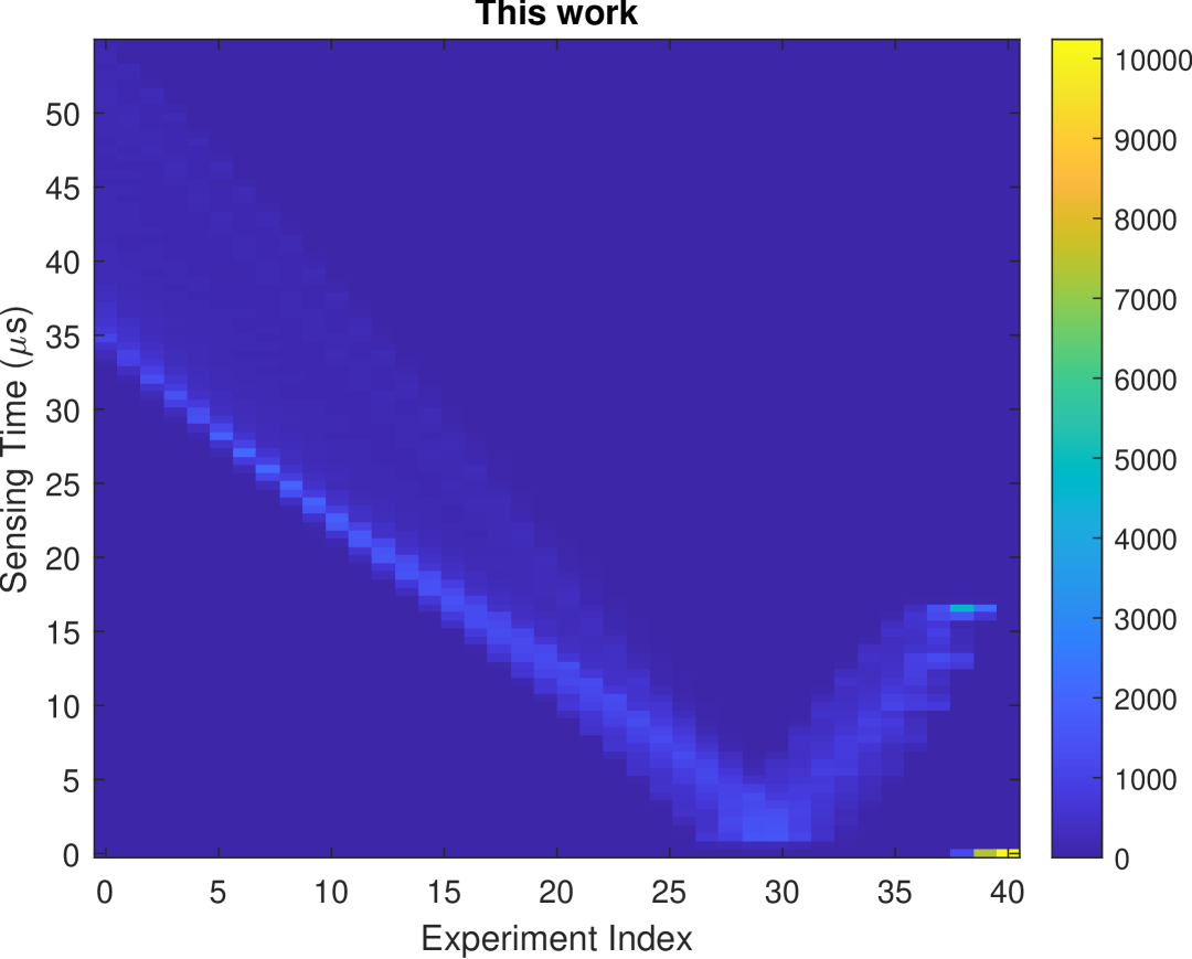
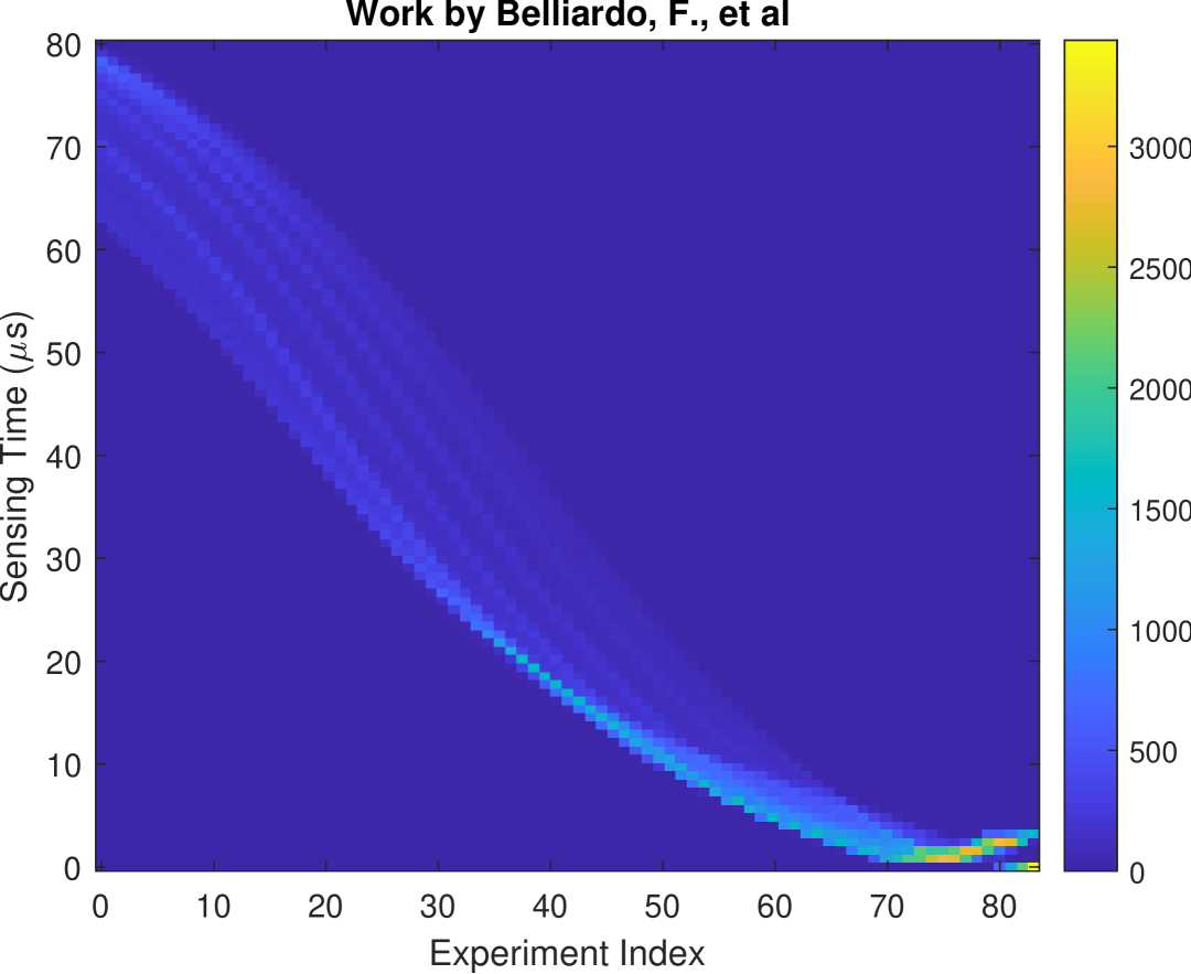
$\omega\in(0,5)$MHz

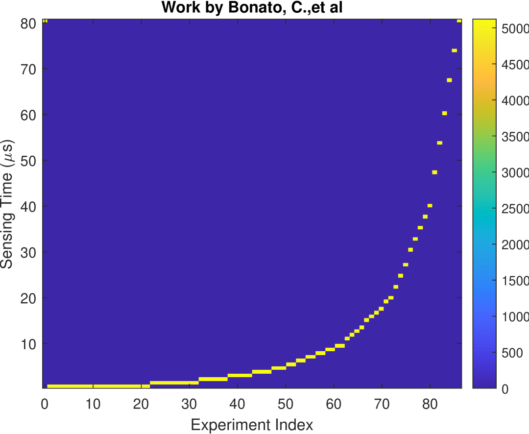
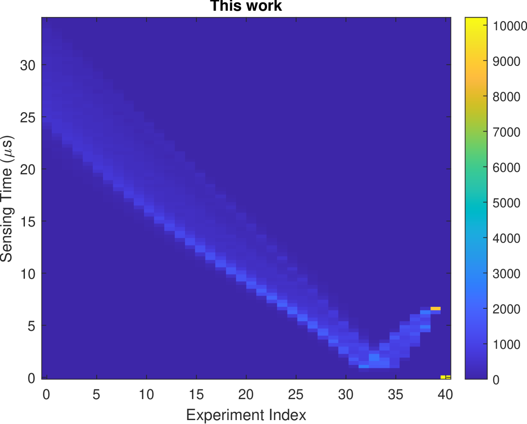
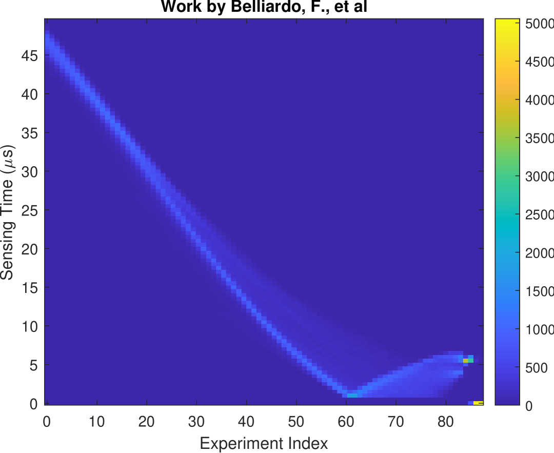
$\omega\in(0,10)$MHz

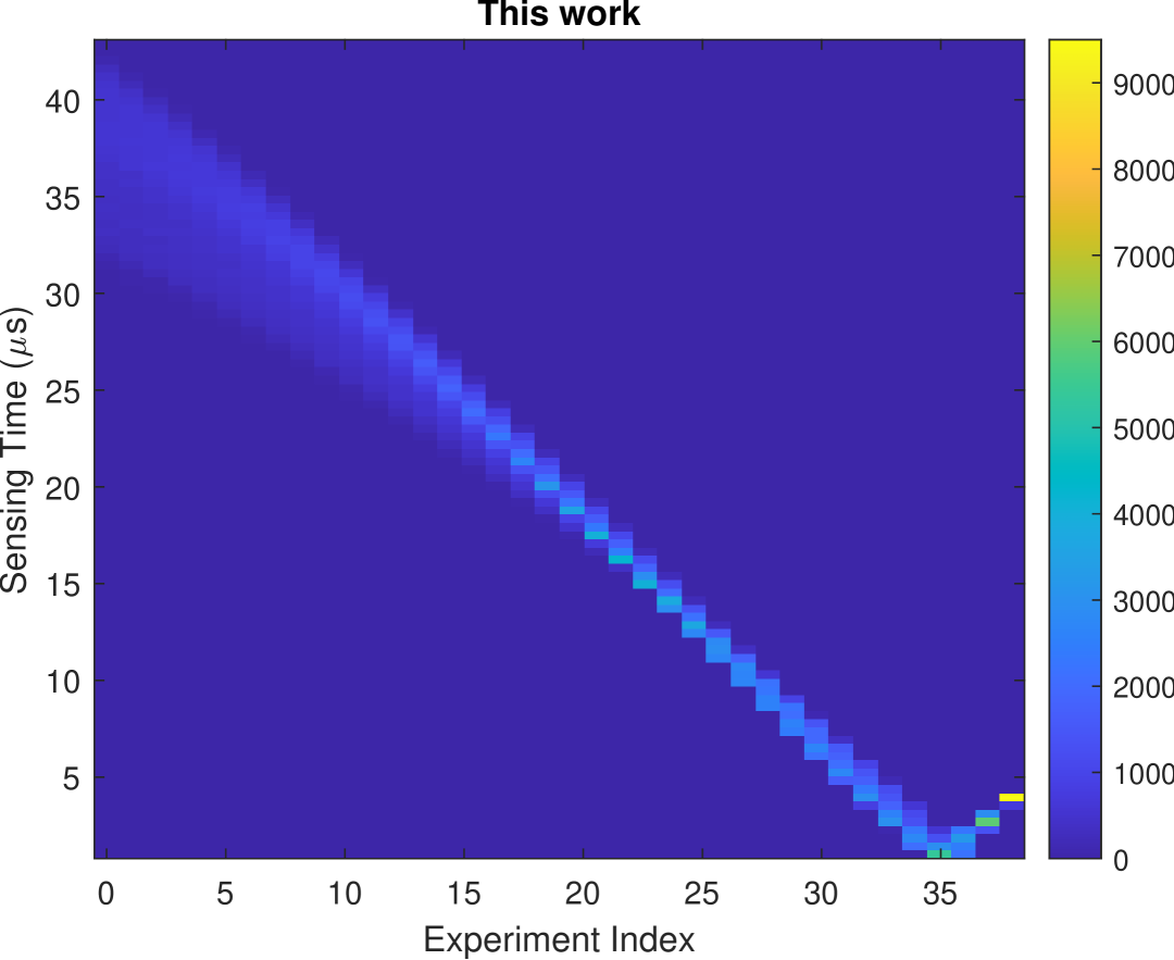
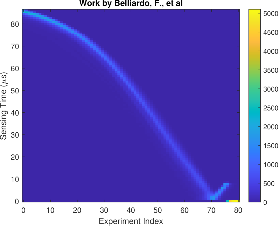
$\omega\in(0,20)$MHz

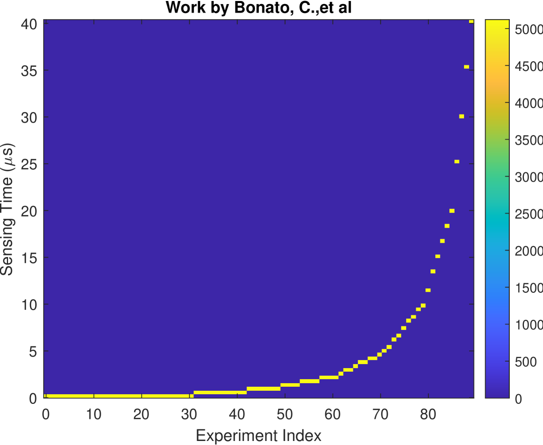
Figure 6: Distribution of optimized sensing time for different protocols

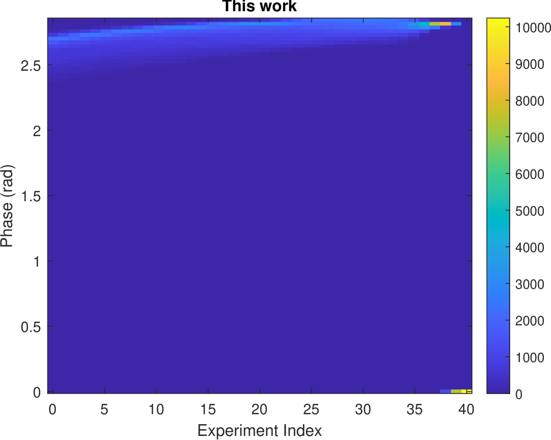
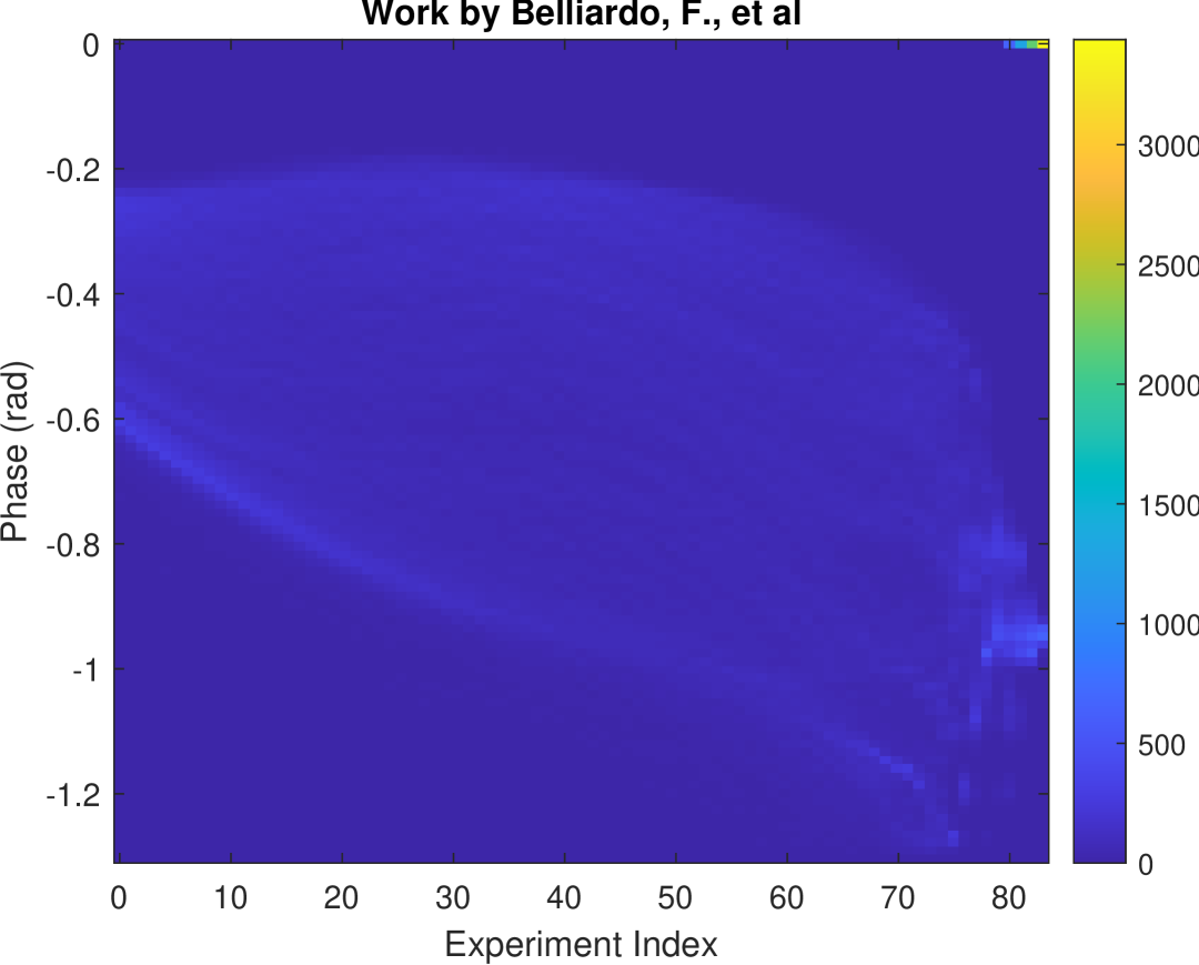
$\omega\in(0,5)$MHz

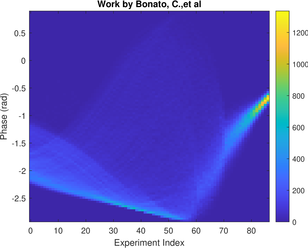
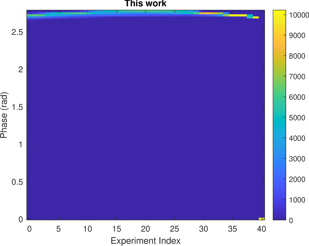
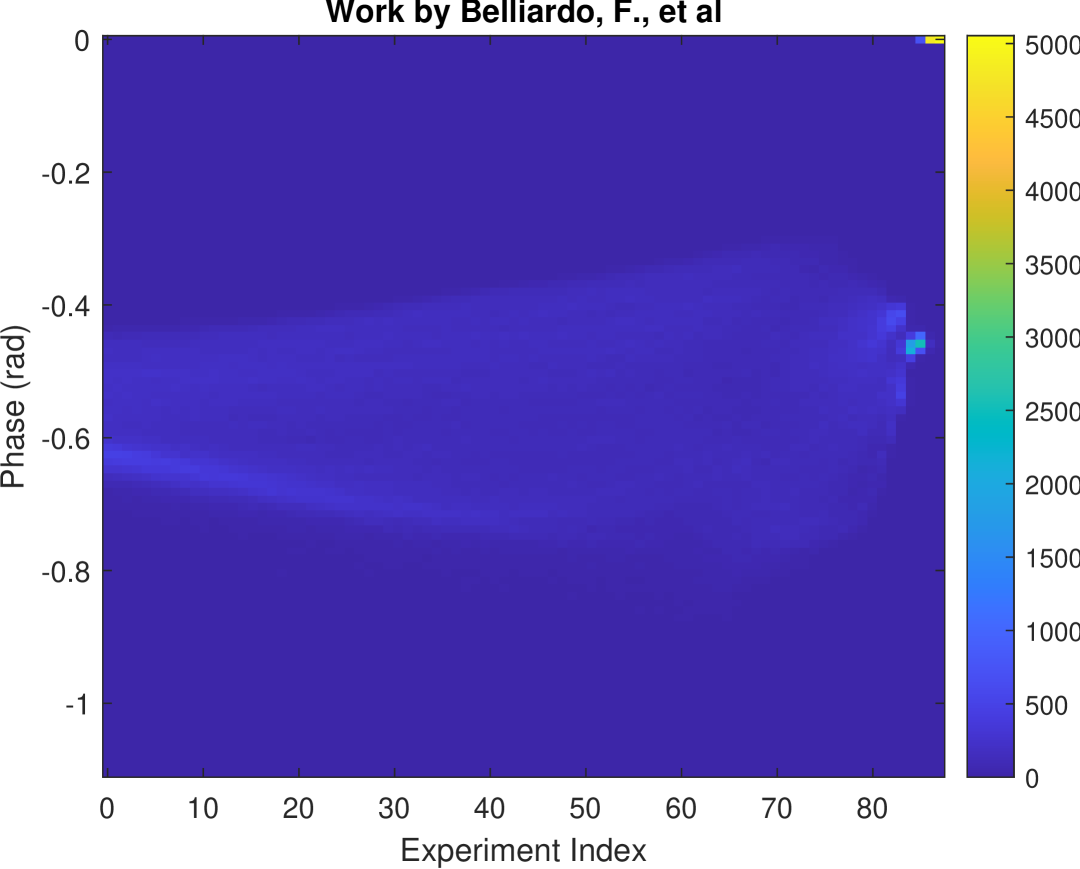
$\omega\in(0,10)$MHz

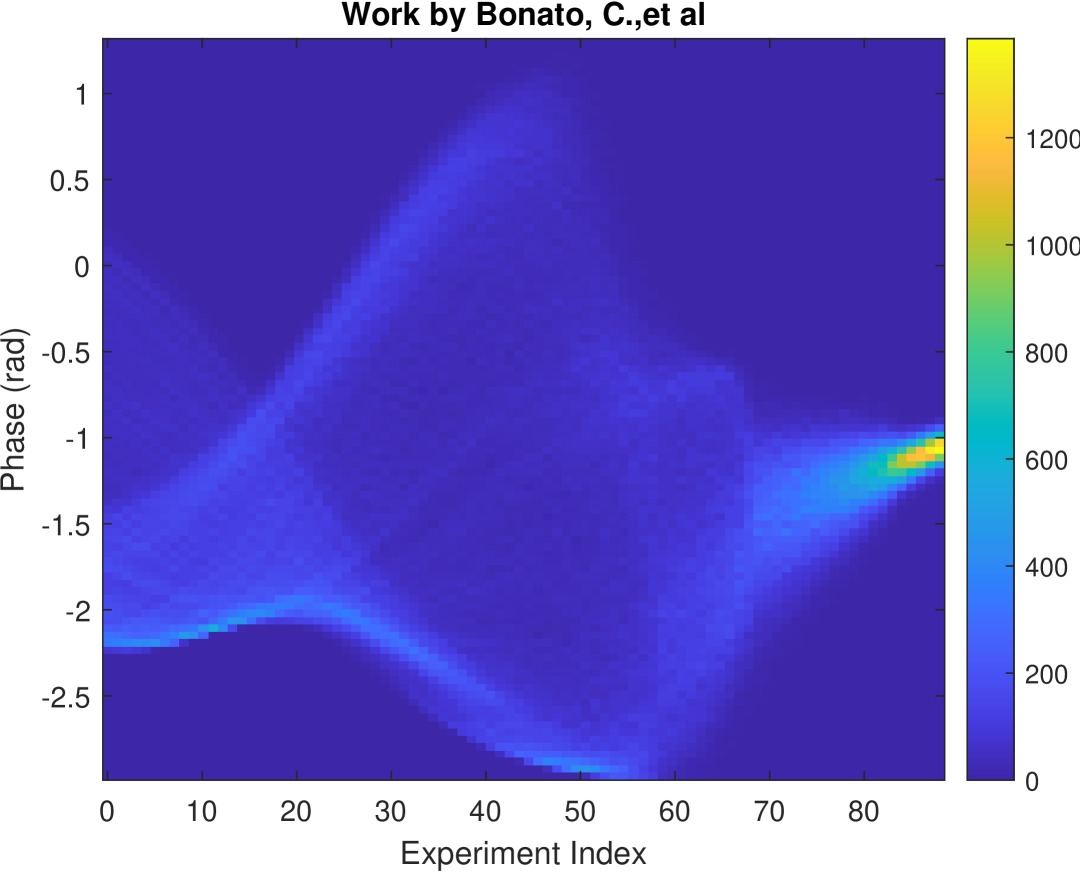
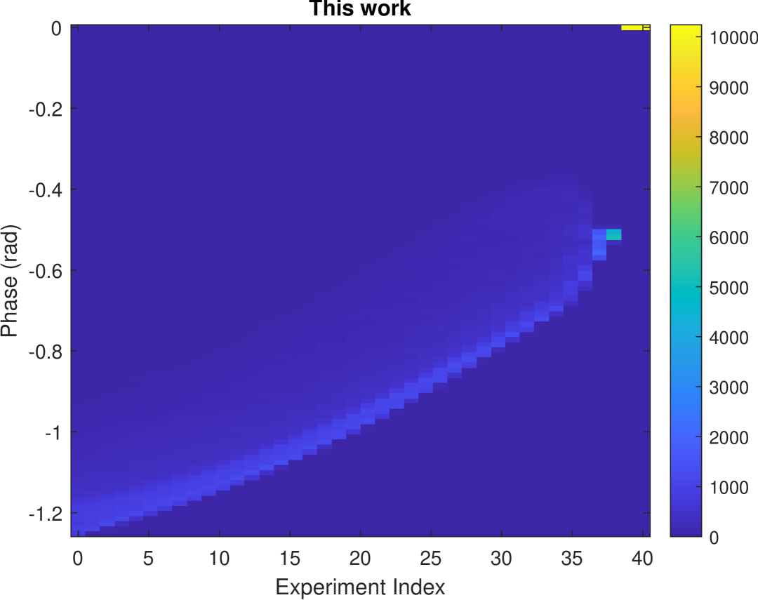
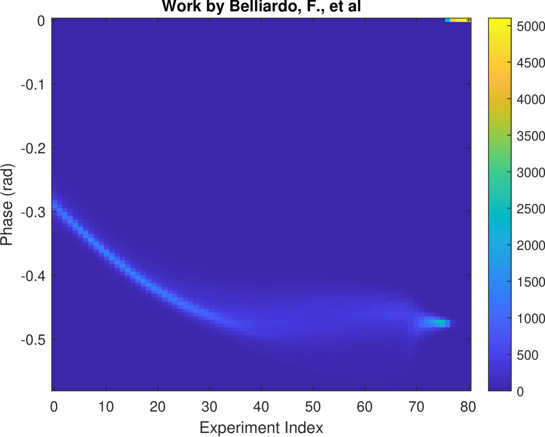
$\omega\in(0,20)$MHz

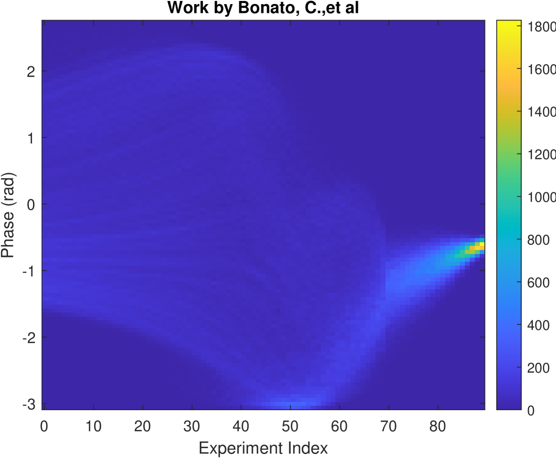
Figure 7: Distribution of optimized control phase for different protocols

Fig. 6 and Fig. 7 show the frequency distributions of the optimized sensing parameters that correspond to the estimation results presented in Fig. 2 and Fig. 3. In Fig. 6, the optimized sensing time of this work’s protocol exhibits a trend similar to that reported by Belliardo et al. [27]. In both cases, the sensing time initially decreases as time resources are dissipated, and then slightly increases near the end of the estimation process as the remaining resources become limited. Nevertheless, the advantage of our protocol is the faster convergence speed as evidenced by the steeper slope and a smaller number of experiments (40 in ours while $>$ 90 in others). This is because the search space of our algorithm is comparably smaller which is in the range of 0-40 $\mu$s, thanks to the narrowed range from the output of the protocol’s $1^{\text{st}}$ Stage. It is also worth to mention that the method by Bonato et al. [12] follows an exponential function to select the sensing time $\tau$. Most of the experiments choose a very small $\tau$ while large values of $\tau$’s are selected very sparsely. This effect is very similar to the method by Nolan et al. [34] in which $\tau$ is fixed as $\tau_{\text{min}}$. This unfortunately results in a significant loss of exploration in the search space. In addition to the sensing time optimization, Fig. 6 shows the distribution of controlled phase $\varphi$ during the runs of the three algorithms. It can be observed that the evolution of $\varphi$ has a stark difference among the three protocols, but they all exhibit convergence toward the final stages of the estimation sequence, as evidenced by the bright point on the far right of each figure. The results in Fig. 7 further confirm that our protocol converges faster.

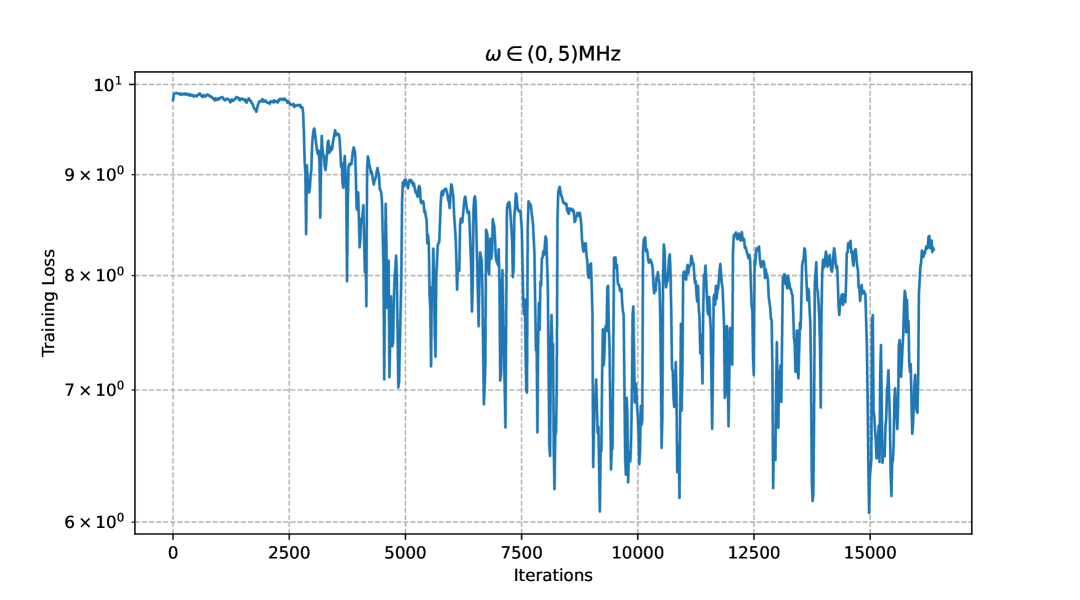
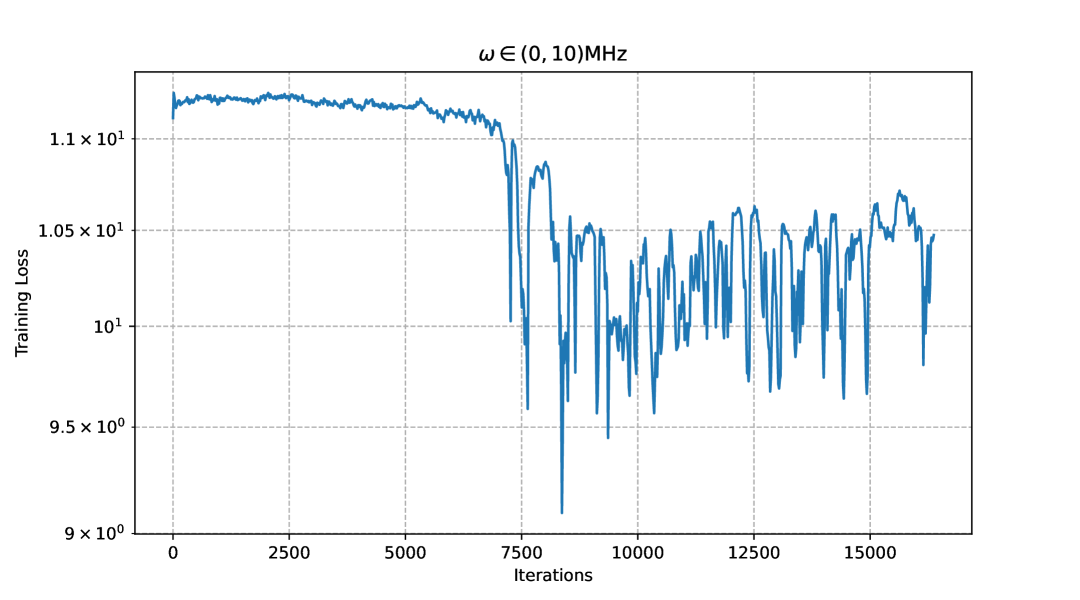
Work by Belliardo, F., et al. [27]

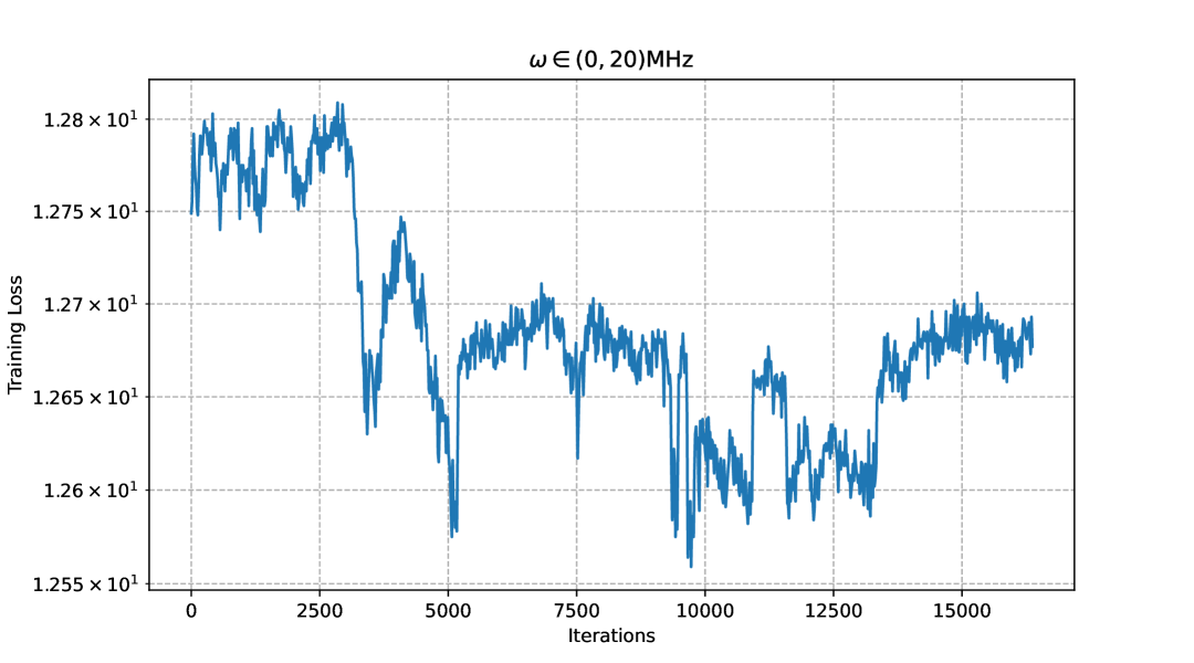
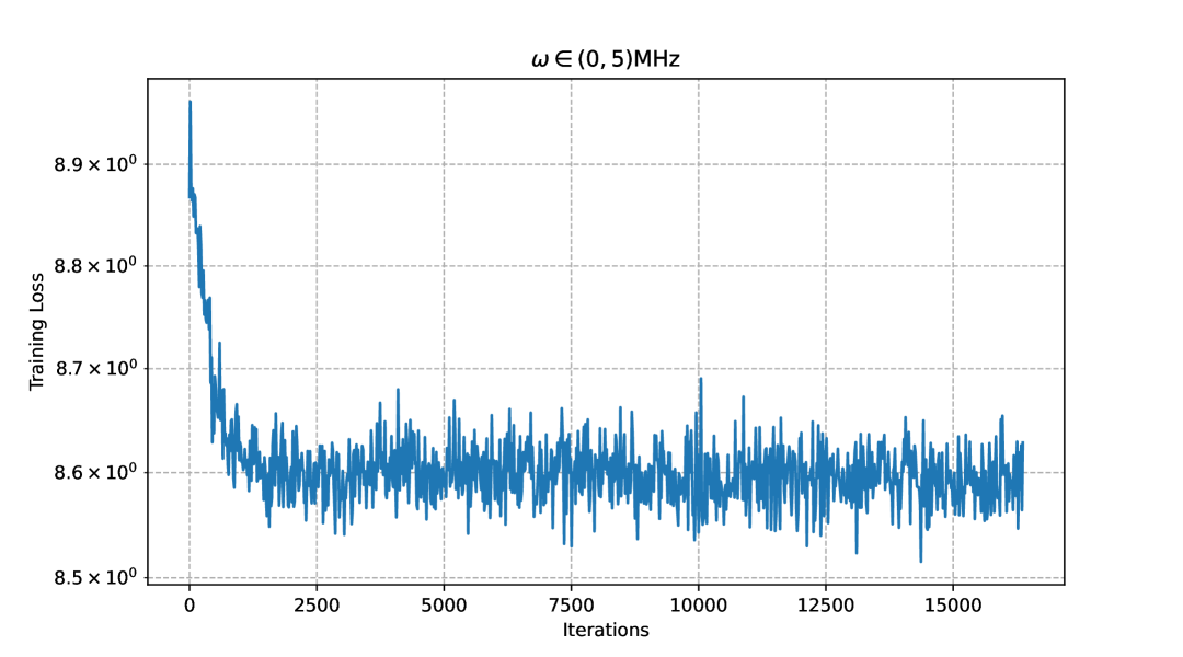
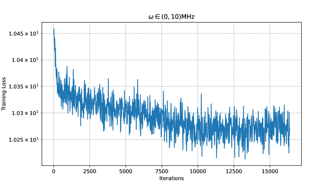
Work by Bonato, C., et al. [12]

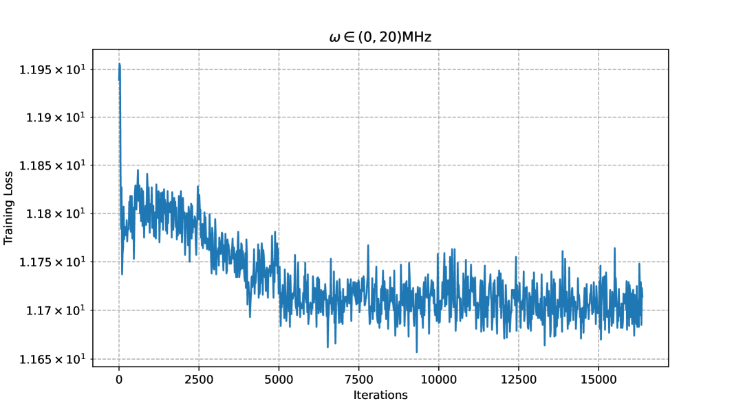
Figure 8: Training loss of the RL agent in the two baseline protocols

To further compare the performance of the two adaptive baseline methods by Belliardo et al. [27] and Bonato et al. [12], we examine the performance of their models in terms of training loss measured by the estimation MSE. Note that the swarm optimization method by Bonato et al. [12] initially used Holevo variance to dictate iterative search of the sensing parameter $\varphi$. To make a fair comparison, we re-implement Bonato’s method using the same RL framework as the one in Belliardo et al. [27]. The changes include but are not limited to using particle filter to approximate the Bayesian posterior probability and using MSE as the loss function. Some exemplary simulation setups are as follows: the number of particles was fixed at $P=960$, and the number of training iterations is set to 16,384. Fig. 8 plots the training loss curves of the two methods. This result can explain the performance of the two methods in Fig. 2 and Fig. 3. Because Bonato’s method only optimizes $\varphi$, its model convergence is much better than Belliardo’s method, particularly when $\omega\in(0,20)$MHz for wide-range sensing. Their training losses in three $\omega$ settings are rather close, with Belliardo’s method having a minor edge for small $\omega$’s.

References

- \bibcommenthead
- Casacio et al. [2021] Casacio, C.A., Madsen, L.S., Terrasson, A., Waleed, M., Barnscheidt, K., Hage, B., Taylor, M.A., Bowen, W.P.: Quantum-enhanced nonlinear microscopy. Nature 594(7862), 201–206 (2021)
- Rondin et al. [2014] Rondin, L., Tetienne, J.-P., Hingant, T., Roch, J.-F., Maletinsky, P., Jacques, V.: Magnetometry with nitrogen-vacancy defects in diamond. Reports on progress in physics 77(5), 056503 (2014)
- Liu et al. [2024] Liu, J., Le, T., Ji, T., Yu, R., Farfurnik, D., Bryd, G., Stancil, D.: The road to quantum internet: Progress in quantum network testbeds and major demonstrations. Progress in Quantum Electronics, 100551 (2024)
- Taylor et al. [2008] Taylor, J.M., Cappellaro, P., Childress, L., Jiang, L., Budker, D., Hemmer, P.R., Yacoby, A., Walsworth, R., Lukin, M.D.: High-sensitivity diamond magnetometer with nanoscale resolution. Nature Physics 4(10), 810–816 (2008)
- Herbschleb et al. [2019] Herbschleb, E., Kato, H., Maruyama, Y., Danjo, T., Makino, T., Yamasaki, S., Ohki, I., Hayashi, K., Morishita, H., Fujiwara, M., et al.: Ultra-long coherence times amongst room-temperature solid-state spins. Nature communications 10(1), 3766 (2019)
- Maletinsky et al. [2012] Maletinsky, P., Hong, S., Grinolds, M.S., Hausmann, B., Lukin, M.D., Walsworth, R.L., Loncar, M., Yacoby, A.: A robust scanning diamond sensor for nanoscale imaging with single nitrogen-vacancy centres. Nature nanotechnology 7(5), 320–324 (2012)
- Dolde et al. [2011] Dolde, F., Fedder, H., Doherty, M.W., Nöbauer, T., Rempp, F., Balasubramanian, G., Wolf, T., Reinhard, F., Hollenberg, L.C., Jelezko, F., et al.: Electric-field sensing using single diamond spins. Nature Physics 7(6), 459–463 (2011)
- Acosta et al. [2010] Acosta, V.M., Bauch, E., Ledbetter, M.P., Waxman, A., Bouchard, L.-S., Budker, D.: Temperature dependence of the nitrogen-vacancy magnetic resonance in diamond. Physical review letters 104(7), 070801 (2010)
- Manson et al. [2006] Manson, N., Harrison, J., Sellars, M.: Nitrogen-vacancy center in diamond: Model of the electronic structure and associated dynamics. Physical Review B—Condensed Matter and Materials Physics 74(10), 104303 (2006)
- Guo [2023] Guo, S.: An overview of nv centers. Journal of Applied Mathematics and Physics 11(11), 3666–3675 (2023)
- Hopper et al. [2018] Hopper, D.A., Shulevitz, H.J., Bassett, L.C.: Spin readout techniques of the nitrogen-vacancy center in diamond. Micromachines 9(9), 437 (2018)
- Bonato et al. [2016] Bonato, C., Blok, M.S., Dinani, H.T., Berry, D.W., Markham, M.L., Twitchen, D.J., Hanson, R.: Optimized quantum sensing with a single electron spin using real-time adaptive measurements. Nature nanotechnology 11(3), 247–252 (2016)
- Taylor and Bowen [2016] Taylor, M.A., Bowen, W.P.: Quantum metrology and its application in biology. Physics Reports 615, 1–59 (2016)
- Giovannetti et al. [2011] Giovannetti, V., Lloyd, S., Maccone, L.: Advances in quantum metrology. Nature photonics 5(4), 222–229 (2011)
- Tóth and Apellaniz [2014] Tóth, G., Apellaniz, I.: Quantum metrology from a quantum information science perspective. Journal of Physics A: Mathematical and Theoretical 47(42), 424006 (2014)
- Morelli et al. [2021] Morelli, S., Usui, A., Agudelo, E., Friis, N.: Bayesian parameter estimation using gaussian states and measurements. Quantum Science and Technology 6(2), 025018 (2021)
- Lee et al. [2022] Lee, K.K., Gagatsos, C.N., Guha, S., Ashok, A.: Quantum-inspired multi-parameter adaptive bayesian estimation for sensing and imaging. IEEE Journal of Selected Topics in Signal Processing 17(2), 491–501 (2022)
- Berritta et al. [2024] Berritta, F., Rasmussen, T., Krzywda, J.A., Van Der Heijden, J., Fedele, F., Fallahi, S., Gardner, G.C., Manfra, M.J., Van Nieuwenburg, E., Danon, J., et al.: Real-time two-axis control of a spin qubit. Nature Communications 15(1), 1676 (2024)
- Salvia et al. [2023] Salvia, R., Mehboudi, M., Perarnau-Llobet, M.: Critical quantum metrology assisted by real-time feedback control. Physical Review Letters 130(24), 240803 (2023)
- MacLellan et al. [2024] MacLellan, B., Roztocki, P., Czischek, S., Melko, R.G.: End-to-end variational quantum sensing. npj Quantum Information 10(1), 118 (2024)
- Xu et al. [2019] Xu, H., Li, J., Liu, L., Wang, Y., Yuan, H., Wang, X.: Generalizable control for quantum parameter estimation through reinforcement learning. npj Quantum Information 5(1), 82 (2019)
- Nolan et al. [2021] Nolan, S.P., Pezze, L., Smerzi, A.: Frequentist parameter estimation with supervised learning. AVS Quantum Science 3(3) (2021)
- McMichael and Blakley [2022] McMichael, R.D., Blakley, S.M.: Simplified algorithms for adaptive experiment design in parameter estimation. Physical review applied 18(5), 054001 (2022)
- Arshad et al. [2024] Arshad, M.J., Bekker, C., Haylock, B., Skrzypczak, K., White, D., Griffiths, B., Gore, J., Morley, G.W., Salter, P., Smith, J., et al.: Real-time adaptive estimation of decoherence timescales for a single qubit. Physical Review Applied 21(2), 024026 (2024)
- Zohar et al. [2023] Zohar, I., Haylock, B., Romach, Y., Arshad, M.J., Halay, N., Drucker, N., Stöhr, R., Denisenko, A., Cohen, Y., Bonato, C., et al.: Real-time frequency estimation of a qubit without single-shot-readout. Quantum Science and Technology 8(3), 035017 (2023)
- Fiderer et al. [2021] Fiderer, L.J., Schuff, J., Braun, D.: Neural-network heuristics for adaptive bayesian quantum estimation. Prx Quantum 2(2), 020303 (2021)
- Belliardo et al. [2024] Belliardo, F., Zoratti, F., Marquardt, F., Giovannetti, V.: Model-aware reinforcement learning for high-performance bayesian experimental design in quantum metrology. Quantum 8, 1555 (2024)
- Cimini et al. [2023] Cimini, V., Valeri, M., Polino, E., Piacentini, S., Ceccarelli, F., Corrielli, G., Spagnolo, N., Osellame, R., Sciarrino, F.: Deep reinforcement learning for quantum multiparameter estimation. Advanced Photonics 5(1), 016005–016005 (2023)
- Metz and Bukov [2023] Metz, F., Bukov, M.: Self-correcting quantum many-body control using reinforcement learning with tensor networks. Nature Machine Intelligence 5(7), 780–791 (2023)
- Fösel et al. [2018] Fösel, T., Tighineanu, P., Weiss, T., Marquardt, F.: Reinforcement learning with neural networks for quantum feedback. Physical Review X 8(3), 031084 (2018)
- Reuer et al. [2023] Reuer, K., Landgraf, J., Fösel, T., O’Sullivan, J., Beltrán, L., Akin, A., Norris, G.J., Remm, A., Kerschbaum, M., Besse, J.-C., et al.: Realizing a deep reinforcement learning agent for real-time quantum feedback. Nature Communications 14(1), 7138 (2023)
- Fallani et al. [2022] Fallani, A., Rossi, M.A., Tamascelli, D., Genoni, M.G.: Learning feedback control strategies for quantum metrology. PRX Quantum 3(2), 020310 (2022)
- Cappellaro [2012] Cappellaro, P.: Spin-bath narrowing with adaptive parameter estimation. Physical Review A—Atomic, Molecular, and Optical Physics 85(3), 030301 (2012)
- Nolan et al. [2021] Nolan, S., Smerzi, A., Pezzè, L.: A machine learning approach to bayesian parameter estimation. npj Quantum Information 7(1), 169 (2021)
- Lehmann and Casella [2006] Lehmann, E.L., Casella, G.: Theory of Point Estimation. Springer, ??? (2006)
- Diederik [2014] Diederik, K.: Adam: A method for stochastic optimization. (No Title) (2014)
- Bradbury et al. [2018] Bradbury, J., Frostig, R., Hawkins, P., Johnson, M.J., Leary, C., Maclaurin, D., Necula, G., Paszke, A., VanderPlas, J., Wanderman-Milne, S., et al.: Jax: composable transformations of python+ numpy programs (2018)