Block-wise Adaptive Caching for Accelerating Diffusion Policy

Abstract

Diffusion Policy has demonstrated strong visuomotor modeling capabilities, but its high computational cost renders it impractical for real-time robotic control. Despite huge redundancy across repetitive denoising steps, existing diffusion acceleration techniques fail to generalize to Diffusion Policy due to fundamental architectural and data divergences. In this paper, we propose Block-wise Adaptive Caching (BAC), a method to accelerate Diffusion Policy by caching intermediate action features. BAC achieves lossless action generation acceleration by adaptively updating and reusing cached features at the block level, based on a key observation that feature similarities vary non-uniformly across timesteps and blocks. To operationalize this insight, we first propose the Adaptive Caching Scheduler, designed to identify optimal update timesteps by maximizing the global feature similarities between cached and skipped features. However, applying this scheduler for each block leads to significant error surges due to the inter-block propagation of caching errors, particularly within Feed-Forward Network (FFN) blocks. To mitigate this issue, we develop the Bubbling Union Algorithm, which truncates these errors by updating the upstream blocks with significant caching errors before downstream FFNs. As a training-free plugin, BAC is readily integrable with existing transformer-based Diffusion Policy and vision-language-action models. Extensive experiments on multiple robotic benchmarks demonstrate that BAC achieves up to $3\times$ inference speedup for free.

1 Introduction

Diffusion Policy has gained substantial attention in robotic control, due to its ability to model action distributions via conditional denoising processes Chi et al. (2023). Recently, it has also been widely adopted by vision-language-action models  Wen et al. (2025); Liu et al. (2025); Hou et al. (2025) to perform highly dexterous and complex tasks. However, its massive computational burden in the denoising process makes the action frequency unable to satisfy real-time and smooth control. For instance, on a 6-DoF robotic arm executing block pick-and-place, 50 diffusion denoising steps at 1 ms per step restrict the action update rate to 10 Hz, well below the 30–50 Hz needed for smooth real-time control Shih et al. (2023).

Despite the aforementioned necessity, the acceleration of Diffusion Policy remains an underexplored field. Cache-based methods have recently gained significant attention in accelerating diffusion models on image-generation tasks Ma et al. (2024a); Wimbauer et al. (2024); Selvaraju et al. (2024); Chen et al. (2024); Zou et al. (2025) and video-generation tasks Liu et al. (2024); Kahatapitiya et al. (2024); Lv et al. (2024). However, they cannot be directly applied to Diffusion Policy, due to differences in data characteristics and model architectures.

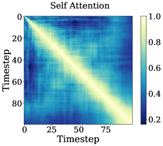
(a) Feature similarities across timesteps.

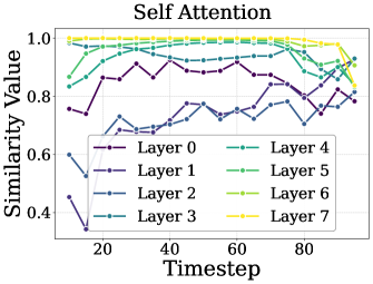
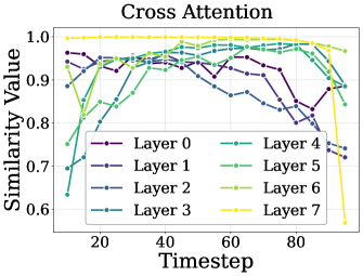
(b) Similarity change curves, measured between timestep $t$ and $t{-}10$.

Figure 1: Temporal and block-wise feature similarity patterns. (a) Similarity matrices of blocks in the third decoder layer. (b) Similarity change curves of different blocks. The feature similarity between consecutive timesteps varies non-uniformly over time and differs across blocks.

To address this issue, we aim to propose a customized feature caching method for Diffusion Policy. We first explore the distinct characteristics of Diffusion Policy models and identify two key observations in feature similarities: (1) feature similarities across timesteps vary non-uniformly, and (2) different blocks exhibit distinct temporal similarity patterns as shown in Fig. 1.

Motivated by this observation, we propose Block-wise Adaptive Caching (BAC), a training-free method that accelerates transformer-based Diffusion Policy by adaptively updating and reusing cached action features at the block level. BAC integrates an Adaptive Caching Scheduler (ACS) to allocate block-specific caching schedules and a Bubbling Union Algorithm (BUA) to truncate inter-block error propagation.

Specifically, the Adaptive Caching Scheduler aims to identify a set of cache update timesteps that maximize the global feature similarities between cached and skipped features. However, directly searching this set within an exponential search space is unacceptable. To address this challenge, we reformulate the problem as a dynamic programming optimization, where the global similarity serves as the objective and the block-specific similarity matrix defines the scores. Leveraging the high episode homogeneity within a single task, the scheduler computes once before inference, incurring virtually no additional cost.

While the Adaptive Caching Scheduler effectively determines update timesteps, extending the scheduler to the block level can trigger significant error surges, leading to performance collapse. We examine this problem theoretically and experimentally and attribute this failure to inter-block caching error propagation: FFN blocks introduce the caching errors from upstream blocks during their updates, due to the lack of intermediate normalization. To truncate the error propagation, we propose the Bubbling Union Algorithm, which first selects the upstream blocks with large caching errors and then enforces them to update their cache if downstream FFNs do.

Our main contributions are as follows:

• We propose Block-wise Adaptive Caching, a training-free acceleration method for transformer-based Diffusion Policy, which adaptively updates and reuses cached features at the block level.

• We develop the Adaptive Caching Scheduler that optimally determines cache update timesteps by maximizing the global feature similarity with a dynamic programming solver.

• We design the Bubbling Union Algorithm to further extend the caching schedule to the block level by truncating inter-block caching error propagation, based on the theoretical and empirical analysis of the error surge phenomenon in Diffusion Policy.

• We conduct extensive robotic experiments to evaluate our method. The results demonstrate that our method efficiently boosts Diffusion Policy by $3\times$ for free.

2 Related Work

2.1 Diffusion Policy

Diffusion models Esser et al. (2024); Bar-Tal et al. (2024) were originally proposed for image generation  Sohl-Dickstein et al. (2015); Ho et al. (2020) and have been adapted for robot policy learning Martinez-Cantin et al. (2007). Traditionally, diffusion-based vision–language–action (VLA) Ma et al. (2024b); Brohan et al. (2023); Kim et al. (2024) methods have depended on U-Net Ronneberger et al. (2015) based denoising backbones borrowed directly from image generation pipelines to model multimodal action distributions and ensure stable training. Within the Diffusion Policy framework  Chi et al. (2023), both U-Net and Diffusion Transformer (DiT) Peebles and Xie (2023); Yuan et al. (2024); Zhao et al. (2024) denoisers are supported, enabling exploration of hybrid backbone designs. More recent work has begun to replace U-Net with DiT architectures to improve scalability and expressive power. Diffusion Transformer Policy  Hou et al. (2024) is itself a DiT variant within the broader Diffusion Policy framework and uses a large-scale Transformer Vaswani et al. (2017) as the denoiser in continuous action spaces, conditioned on visual observations and language instructions. The Diffusion-VLA framework  (Wen et al., 2024) unifies autoregressive next-token reasoning with diffusion-based action generation into a single, scalable framework for fast, interpretable, and generalizable visuomotor robot policies. DexVLA Wen et al. (2025) introduces plug-in diffusion expert modules that decouple action generation from the core VLA backbone. However, the iterative denoising steps inherent in diffusion models introduce substantial inference latency that poses challenges for high-frequency VLA tasks requiring real-time responsiveness. Consequently, accelerating the inference procedure of diffusion-based policies through techniques such as caching Xu et al. (2025); Song et al. (2025) is critical for deploying responsive VLA-driven agents Chiang et al. (2024); Xiang et al. (2025); Li et al. (2025).

2.2 Diffusion Models Caching

Despite the success of cache-based methods for diffusion models, their adaptation to Diffusion Policy remains underexplored. Existing caching methods primarily target U-Net-based diffusion models Ma et al. (2024a); Wimbauer et al. (2024). For example, DeepCache Ma et al. (2024a) exploits the temporal redundancy inherent in U-Nets by caching high-level feature representations. Nevertheless, these methods cannot be generalized to transformer backbones. Recently, some methods Selvaraju et al. (2024); Ma et al. (2024c); Chen et al. (2024); Zou et al. (2025) explore the caching mechanism in transformer-based diffusion models. These methods typically operate at a coarse granularity, with all the blocks sharing a uniform caching schedule Selvaraju et al. (2024); Ma et al. (2024a), i.e., updating the cache at uniform intervals. Despite some works extending this schedule in a finer architectural granularity, they either require extra training Ma et al. (2024c) or are specifically designed for the patterns of the image generation process Chen et al. (2024).

3 Block-wise Adaptive Caching

As illustrated in Fig. 2, BAC achieves a finer-grained cache schedule by first applying the Adaptive Caching Scheduler to compute optimal update timesteps for each block and then employing the Bubbling Union Algorithm to truncate inter-block error propagation. In this section, we first present the preliminaries in Sec. 3.1. Next, we introduce the Adaptive Caching Scheduler in Sec. 3.2. To extend the scheduler to the block level, we analyze the error surge phenomenon in Sec. 3.3 and describe the Bubbling Union Algorithm in Sec. 3.4.

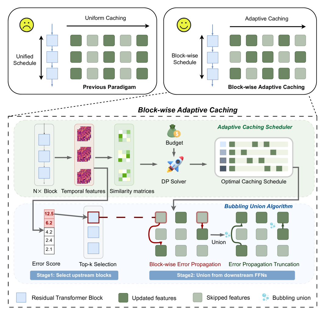
Figure 2: Framework of Block-wise Adaptive Caching (BAC). BAC enables adaptive feature caching by introducing the Adaptive Caching Scheduler, and further supports block-wise scheduling through the Bubbling Union Algorithm.

3.1 Preliminaries

Diffusion Policy.

Diffusion Policy treats robot visuomotor control as sampling from a conditional denoising diffusion model (Chi et al., 2023). At each time step $t$, we first draw an initial noisy action $\mathbf{a}_{t}^{(K)}$ from a standard Gaussian prior and then apply $K$ learned reverse-diffusion steps:

$$\mathbf{a}_{t}^{(k-1)}=f_{\theta}\bigl{(}\mathbf{a}_{t}^{(k)},\,\mathbf{o}_{1:t},\,k\bigr{)},\quad k=K,\,K-1,\,\dots,\,1,$$ (1)

where $f_{\theta}$ parameterizes the conditional reverse kernel (i.e. the denoiser) and the final sample $\mathbf{a}_{t}^{(0)}$ is used as the control action.

Diffusion Transformer (DiT).

The DiT architecture in Diffusion Policy utilizes an MLP to encode observation embeddings, which are then passed into a transformer-based decoder. The decoder consists of $L$ layers, where each layer $l$ contains a cross-attention (CA) block that conditions on timesteps and observations, a self-attention (SA) block, and a feed-forward network (FFN) block. For a given input $\mathbf{h}_{k}^{(l-1)}$ at denoising step $k$, the output of layer $l$ is computed by summing the residual outputs of these blocks:

$$\mathbf{h}_{k}^{(l)}=\mathbf{h}_{k}^{(l-1)}+\text{SA}_{k}^{(l)}+\text{CA}^{(l)}_{k}+\text{FFN}_{k}^{(l)}.$$ (2)

Problem Formulation.

To reduce redundant computations across timesteps in the denoising process of diffusion models, cache-based methods reuse intermediate features to skip repeated computations partially. Following existing caching methods (Ma et al., 2024a; Selvaraju et al., 2024), we adopt an update-then-reuse paradigm.

Let $\mathbf{b}_{k}$ denote the output of a target block at step $k$. A caching mechanism defines a set of update steps $\mathcal{C}\subseteq\{1,\dots,K\}$, where:

• The update step: If $k\in\mathcal{C}$, computes $\mathbf{b}_{k}$ and updates its cached features.

• The reuse step: The block reuses the cached feature $\mathbf{b}_{k^{\prime}}$, which is computed in the most recent update step $k^{\prime}=\min\{i\in\mathcal{C}\mid i>k\}$.

Following prior work  (Zou et al., 2025; Selvaraju et al., 2024; Ma et al., 2024a), we construct a baseline in which all blocks share a unified caching schedule, with a fixed update interval $\mathcal{C}$ (e.g., updating the cache every three timesteps). BAC aims to improve upon this baseline by allocating an optimal $\mathcal{C^{*}}$ for each block.

3.2 Adaptive Caching Scheduler

Optimization Objective.

In this work, we use cosine similarity to measure the similarity between features due to its superior performance in measuring directional consistency between high-dimensional feature vectors. The consecutive similarity is calculated as:

$$s_{k}=\cos(\mathbf{b}_{k},\mathbf{b}_{k-1})=\frac{\mathbf{b}_{k-1}^{\top}\mathbf{b}_{k}}{\|\mathbf{b}_{k-1}\|_{2}\|\mathbf{b}_{k}\|_{2}},\quad k=1,\dots,K,$$ (3)

We define the interval similarity between timesteps $i$ and $j$ as $\phi(i,j)=\sum_{k=i+1}^{j}s_{k}$. A larger $\phi(i,j)$ indicates lower caching errors incurred by reusing the cached feature $b_{j}$ over the interval $[i,j]$. The value function is then:

$$\max_{\begin{subarray}{c}\mathcal{C}\subseteq\{1,\dots,K\}\\ |\mathcal{C}|=M\end{subarray}}\sum_{m=0}^{M}\phi(c_{m},c_{m+1}-1),\quad\text{with}\quad c_{0}=0,\quad c_{M+1}=K,$$ (4)

where $c_{0}$ and $c_{M+1}$ are boundary conditions representing the start step and the end step of the path.

Optimal Schedule Solver.

The combinatorial nature of selecting $M$ update steps from $K$ timesteps renders exhaustive search computationally infeasible for large $K$. To address this, we design a dynamic programming (DP) solver that efficiently computes the optimal cache schedule.

Define the DP state $\text{DP}[m][j]$ as the maximum cumulative similarity achievable when the $m$-th cache update occurs at timestep $j$:

$$\mathrm{DP}[m][j]=\max\sum_{i=0}^{m}\phi\bigl{(}c_{i},\;c_{i+1}-1\bigr{)}.$$ (5)

The corresponding state transition equation is given by:

$$\text{DP}[m][j]=\max_{0\leq i<j}\left\{\text{DP}[m-1][i]+\phi(i,j)\right\},$$ (6)

To recover the optimal update schedule $\mathcal{C}^{*}$ from the DP table, we introduce a pointer matrix:

$$\mathrm{PTR}[m][j]=\arg\max_{0\leq i<j}\bigl{\{}\mathrm{DP}[m-1][i]+\phi(i,j)\bigr{\}},\quad m=1,\dots,M,\;j=1,\dots,K.$$ (7)

Once both $\mathrm{DP}$ table and $\mathrm{PTR}$ table are filled, we dertermine the final endpoint as:

$$j^{*}=\arg\max_{1\leq j\leq K}\mathrm{DP}[M][j],$$ (8)

and backtrack from $j^{*}$ to reconstruct the full update schedule:

$$c_{M}^{*}=j^{*},\quad c_{m-1}^{*}=\mathrm{PTR}[m][\,c_{m}^{*}\,],\quad m=M,\dots,1.$$ (9)

The solved optimal update step set is given by $\mathcal{C}^{*}=\{c_{1}^{*}<\dots<c_{M}^{*}\}$. Adaptive Caching Scheduler maximizes the performance efficiency trade-off by computing $\mathcal{C^{*}}$ for each block under the given computation budget.

3.3 The Error Surge Phenomenon and Analysis.

However, purely extending the Adaptive Caching Scheduler to the block level can trigger significant error surges, particularly within FFN blocks. We provide a detailed analysis of this failure mode in the following section and introduce our remedy Bubbling Union Algorithm in Sec. 3.4.

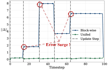
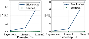
(a)

(b)

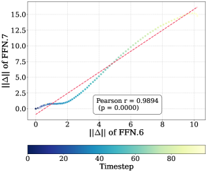
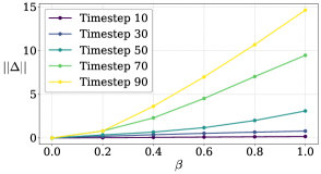
(c)

(d)

(e)

Figure 3: (a) Caching error of the third FFN block when updated using the block-wise versus a unified schedule. (b) Caching error of sub-layers within the third FFN block at update timesteps 14 and 31. (c) Correlation between the caching errors of the seventh and eighth FFN blocks. (d) Update-induced error under varying input error magnitudes, controlled by the scaling factor $\beta$. (e) Caching error across all blocks throughout the diffusion process, with white dots indicating update steps. All experiments are conducted on the Square task.

Identifying Error Surge.

Extending Adaptive Caching Scheduler to the block level leads to unexpected performance collapse (See Table 2). Our observation uncovers a surprising phenomenon: instead of reducing errors, block-wise updates amplify them, resulting in sudden error surges in the FFN blocks, as illustrated in Fig. 3.

Generally, caching errors arise from either feature reuse or feature update. In the reuse case, the error comes from a mismatch between cached features and the shifted ground-truth distribution. In the update case, the error results from inaccurate inputs caused by errors from upstream blocks. We observe that error surges often occur during update steps of FFN blocks, where update-induced errors exceed reuse-induced errors, indicating a failure in the update process. We first elucidate how FFN blocks incorporate these upstream errors during updates, then delineate the complete inter-block error propagation process.

Error Propagation in FFN Blocks.

To understand how FFN blocks incorporate the upstream errors, we begin by formalizing the error propagation process. Let

$$\mathrm{FFN}(X)=W_{\mathrm{out}}\phi(W_{\mathrm{in}}\mathrm{LN}(X)+b_{1})+b_{2},$$ (10)

Proposition 3.1.

Given an upstream error $\delta$, we have

$$\Delta=W_{\mathrm{out}}\,\mathrm{diag}\bigl{(}\phi^{\prime}(U)\bigr{)}\,W_{\mathrm{in}}\,(A-B)\,\delta+O(\|\delta\|^{2}),$$ (11)

where

$$A=\frac{\operatorname{diag}(\gamma)\,\bigl{(}I-\tfrac{1}{d}\mathbf{1}\mathbf{1}^{\top}\bigr{)}}{\sigma(X)},\quad B=\frac{\operatorname{diag}(\gamma)\,(X-\mu(X)\mathbf{1})(X-\mu(X)\mathbf{1})^{\top}}{d\,\sigma(X)^{3}}.$$ (12)

To further analyze the correlation between inter-block errors, we design a toy experiment where the upstream block (FFN.6) uses only cached activations, while the downstream block (layer.7.FFN) performs full computation. The relationship between the update-induced error and its corresponding upstream error is depicted in Fig. 3, with a Pearson correlation coefficient of $r=0.9894$, indicating a strong correlation. To isolate the influence of the timestep, we fix it and use a factor $\beta$ to control the magnitude of the upstream error. The result in Fig. 3 also shows a strong positive correlation between upstream and downstream errors, further confirming the effect of inter-block error propagation.

Inter-block Error Propagation.

A complete propagation chain is shown in Fig. 3. When a block updates at a timestep when its upstream block does not update and has a larger caching error, an error surge occurs, visually manifested by a sudden deepening of block colors without any gradual transition. Although the upstream block updates later, the surging error in the downstream block still persists, indicating the failure of this update.

3.4 Bubbling Union Algorithm

To truncate inter-block error propagation, we propose a simple yet effective algorithm to revise the original scheduler. The core insight of our algorithm is that if an FFN block updates its cache, its upstream blocks with large errors should also update. Therefore, the updated error $\Delta$ can be mitigated due to the suppressed propagated upstream error $\delta$.

Our algorithm consists of two stages:

Stage 1: Selecting Upstream Blocks with Large Caching Errors. To estimate the caching error magnitude for each block $j$, we compute the average of $\ell_{1}$ norm across features over all pairs of denoising timesteps:

$$\ell_{j}\;=\;\frac{1}{K^{2}}\sum_{t=1}^{K}\sum_{u=1}^{K}\bigl{\lVert}X_{j}^{(t)}-X_{j}^{(u)}\bigr{\rVert}_{1}\,.$$ (13)

A larger $\ell_{j}$ indicates that the block has larger reuse-induced errors. We then select the top $k$ blocks with the largest $\ell_{j}$ and denote this block set by $U$.

Remark 3.1.

As discussed in Sec. 3.3, caching error consists of both reuse-induced errors and update-induced errors. We choose not to account for the update-induced error of upstream blocks because it occurs less frequently and is difficult to approximate reliably. Moreover, incorporating it would require treating all FFN blocks as upstream blocks, which would compromise the overall trade-off between efficiency and precision.

Stage 2: Unioning Update Timesteps of FFNs from Downstream to Upstream. Our algorithm truncates error propagation by enforcing that each upstream block in $U$ updates its cache before its downstream FFN blocks. Concretely, let $C(u)$ denote cache update timesteps set of block $u$. Let $\mathrm{D}(u)$ be the set of all FFN blocks downstream of block $u$. Then for each $u\in U$, we update $C(u)$ as:

$$C(u)=C(u)\cup\bigcup_{v\in\mathrm{D}(u)}C(v)$$ (14)

4 Experiments

We first outline the experimental setup, covering models, benchmarks, metrics, and implementation details in Sec. 4.1. Following that, we demonstrate the experimental results in Sec. 4.2. Finally, we present an ablation study of BAC in Sec. 4.3.

4.1 Experimental Setup

Models, Benchmarks and Metrics. Following the original settings in Diffusion Policy (Chi et al., 2023), we select the transformer-based Diffusion Policy (DP-T) for our evaluation. The pretrained checkpoints are from . BAC is implemented as a plugin module that can be invoked with a single line of code. We evaluate BAC on DP-T across four different robot manipulation benchmarks with fixed seeds: Robomimic, Push-T, Multimodal Block Pushing, and Kitchen. Demonstration data is sourced from proficient human (PH) and mixed proficient/non-proficient human (MH) teleoperation, as well as scripted Markovian policies (e.g., Block Pushing). For most tasks, the primary precision metric is Success Rate, while Push-T uses target area coverage instead. Efficiency is measured in terms of FLOPs and Speedup during action generation.

Baseline. We report the result of DP-T as Full Precision and utilize the baseline constructed in Sec. 3.1, in which all blocks update and reuse their cache at uniform intervals simultaneously. We refer to this baseline as Uniform.

Implementation Details. We set the hyperparameter $k$ as 5 in all the experiments. The experiments were conducted on a workstation equipped with an NVIDIA GeForce RTX 4090D 24 GB GPU.

Table 1: Results on different benchmarks. We present success rates of different checkpoints in the format of (max performance) / (average of last 10 checkpoints), with each averaged across 3 training seeds. The overall average success rate is denoted as AVG, with average flops and speedup reported as FLOPs and Speed$\times$, respectively.

Benchmark on Proficient Human (PH) demonstration data.

Method	Success Rate $\uparrow$						AVG	FLOPs	Speed $\times$
	Lift	Can	Square	Transport	Tool	Push–T
Full Precision	1.00/1.00	0.95/0.97	0.82/0.88	0.78/0.81	0.43/0.53	0.59/0.64	0.76	15.77G	–
Uniform($\mathcal{S}=7$)	0.82/1.00	0.27/0.78	0.65/0.81	0.77/0.77	0.08/0.68	0.48/0.61	0.65	1.49G	3.59
Uniform($\mathcal{S}=10$)	0.95/0.99	0.39/0.81	0.66/0.88	0.71/0.73	0.04/0.53	0.57/0.67	0.67	1.94G	3.46
yellow!10BAC($\mathcal{S}=7$)	1.00/1.00	0.90/0.95	0.78/0.87	0.75/0.81	0.36/0.47	0.57/0.61	0.74	2.02G	3.54
yellow!10BAC($\mathcal{S}=10$)	1.00/1.00	0.94/0.97	0.82/0.89	0.77/0.82	0.49/0.55	0.59/0.62	0.79	2.66G	3.40

Benchmark on Mixed Human (MH) demonstration data.

Method	Success Rate $\uparrow$				AVG	FLOPs	Speed $\times$
	Lift	Can	Square	Transport
Full Precision	0.99/1.00	0.92/0.97	0.76/0.79	0.35/0.46	0.76	15.77G	–
Uniform($\mathcal{S}=7$)	0.47/1.00	0.34/0.90	0.64/0.72	0.00/0.00	0.51	1.49G	3.60
Uniform($\mathcal{S}=10$)	0.71/1.00	0.35/0.83	0.68/0.61	0.00/0.00	0.53	1.94G	3.49
yellow!10BAC($\mathcal{S}=7$)	0.96/0.99	0.39/0.79	0.56/0.53	0.17/0.41	0.60	2.03G	3.48
yellow!10BAC($\mathcal{S}=10$)	0.99/0.98	0.95/0.97	0.77/0.79	0.30/0.46	0.77	2.64G	3.41

Benchmark on multi-stage tasks. For Block-Pushing, px is the frequency of pushing x blocks into the targets. For Kitchen, px is the frequency of interacting with x or more objects (e.g. bottom burner).

Method	Success Rate $\uparrow$						AVG	FLOPs	Speed $\times$
	BPp1	BPp2	Kitp1	Kitp2	Kitp3	Kitp4
Full Precision	0.98/0.98	0.98/0.96	1.00/1.00	0.98/1.00	0.97/1.00	0.95/0.97	0.98	15.77G	–
Uniform($\mathcal{S}=7$)	0.99/0.99	0.94/0.91	0.20/0.29	0.02/0.07	0.01/0.03	0.01/0.01	0.36	1.49G	4.09
Uniform($\mathcal{S}=10$)	0.99/0.99	0.92/0.91	0.29/0.37	0.05/0.08	0.01/0.03	0.00/0.00	0.38	1.94G	3.70
yellow!10BAC ($\mathcal{S}=7$)	0.99/0.99	0.91/0.93	0.80/0.85	0.61/0.69	0.45/0.57	0.23/0.39	0.69	1.92G	3.78
yellow!10 BAC($\mathcal{S}=10$)	1.00/0.99	0.97/0.95	1.00/0.99	1.00/0.99	1.00/0.99	0.94/0.97	0.98	2.44G	3.60

4.2 Main Results

In Sec. 4.2, we demonstrate the effectiveness of our proposed BAC. We compare BAC against the baselines across multiple benchmarks in Table 1. We control the computation budget by setting the number of cache update steps $S$. BAC achieves lossless acceleration with $S=10$ on all the benchmarks, with an average success rate of 0.79,0.77,0.98 versus 0.76,0.76,0.98 for the full-precision DP-T, even exhibiting a modest improvement. BAC consistently achieves stable acceleration rates above $3.4\times$ across most of the tasks. Compared with Uniform, BAC has two advantages: (1) BAC improves the success rate significantly on the hard tasks such as $\text{Transport}_{mh}$ and $\text{Kitchen}_{p4}$, where Uniform fails to restore the correct action generation. (2) BAC maintains a strong and stable performance in all tasks, demonstrating the reliability of a lossless acceleration plugin. We attribute this to BAC’s ability to reduce the reuse-induced error by ACS and precisely avoid the update-induced errors by BUA.

4.3 Ablation Study

To verify the effectiveness of each component of our method, we conduct ablation experiments on these benchmarks. The selected results on PH benchmark is shown on Table 2.

Ablation Study Methods

We consider three variants of our caching method. To evaluate the effectiveness of ACS, we build Unified ACS, the Adaptive Caching Scheduler is applied solely to the self-attention block in layer 0, which is the very first block in the decoder. The computed update steps are then used by every block. To evaluate the effectiveness of BUA, we build Block-wise ACS, the scheduler is naively applied to each block, producing a distinct set of update steps for all blocks. Finally, in Block-wise ACS + BUA, we first compute block-wise update steps via the Adaptive Caching Scheduler and then integrate the Bubbling Union Algorithm, yielding our full BAC method.

Effectiveness of ACS.

Experiments with the Unified ACS schedule demonstrate a clear performance improvement over Uniform, achieving an average success rate of 0.72 versus 0.65 for Uniform. This result confirms the necessity and effectiveness of reducing the reuse-induced error.

Effectiveness of BUA.

Extending ACS to operate on each block individually yields improvements on some tasks, however, performance falls below that of the full-precision baseline, and in some more challenging cases (e.g., Tool_ph) even collapses, this behavior is consistent with the Error Surge Phenomenon we described in Sec. 3.3, whereby block-wise scheduling can cause downstream blocks to be updated before upstream ones, inducing an error surge and resulting in performance degradation.

Integrating the Bubbling Union Algorithm into the block-wise schedule recovers full-precision performance across all tasks with the highest score of 0.79. This result empirically substantiates the Error Surge Phenomenon and confirms that Bubbling Union Algorithm effectively solves the error surge phenomenon.

Table 2: Ablation Study on BAC

Method	Success Rate $\uparrow$					AVG	FLOPs	Speed $\times$
	Liftph	Canph	Squareph	Toolph	Push–T
Uniform	0.95/0.99	0.39/0.81	0.66/0.88	0.04/0.53	0.57/0.67	0.65	1.94G	3.46
Unified ACS	1.00/1.00	0.63/0.89	0.63/0.83	0.27/0.64	0.50/0.62	0.72	1.94G	3.43
Block-wise ACS	0.77/0.93	0.88/0.83	0.78/0.87	0.03/0.05	0.49/0.56	0.65	1.94G	3.41
yellow!10 Block-wise ACS + BUA	1.00/1.00	0.94/0.97	0.82/0.89	0.49/0.55	0.59/0.62	0.79	2.66G	3.40

5 Limitation

The primary limitation of our work arises when the base model’s accuracy on a given task is very low, as our caching strategy may inadvertently amplify this inaccuracy. For example, on the $\text{Transport}_{mh}$ benchmark, we observe a slight drop in performance. Another limitation is that due to equipment constraints, we have not yet conducted real-world VLA experiments, we plan to address this in future.

6 Conclusion

In this paper, we propose BAC, a novel training-free acceleration method for transformer-based Diffusion Policy. BAC minimizes the caching error by adaptively scheduling cache updates through the Adaptive Caching Scheduler. Moreover, we conduct theoretical and empirical analysis on the error surge phenomenon due to inter-block error propagation, and propose the Bubbling Union Algorithm to truncate the propagation. Extensive experiments demonstrate that BAC achieves substantial speedups without performance degradation, typically exceeding $3\times$ compared to full computation.

Appendix A Appendix / supplemental material

In this supplemental material, we provide complete proofs of Proposition 3.1 in Appendix A.1, along with additional experiments examining the choice of parameter $k$ in Appendix A.3. We further include ablation studies analyzing different metrics in Appendix A.4, and present more temporal similarity figures in Appendix A.5. Additionally, Appendix A.6 contains illustrations demonstrating episode homogeneity within individual tasks, while Appendix A.7 offers supplementary visualizations supporting Figure 3. Finally, in Appendix A.8 and Appendix A.9, we present the update steps obtained under $S=10$, $k=5$, while using cosine as metric via BAC, showing the update steps obtained after employing ACS and BUA, respectively.

A.1 Proof for Proposition 3.1

Assumption A.1.

1. Activation function $\phi$ is twice continuously differentiable with bounded second derivative

2. LayerNorm variance $\sigma(X)\geq\sigma_{\min}>0$ for all valid inputs $X$

3. Weight matrices satisfy $\|W_{1}\|_{2}\leq C_{1}$, $\|W_{2}\|_{2}\leq C_{2}$ for fixed constants $C_{1},C_{2}$

Proposition A.1.

Under Assumption 1, for input error $\delta$ with $\|\delta\|\leq\epsilon$, the FFN block output error admits the first-order approximation:

$$\mathrm{FFN}(X+\delta)-\mathrm{FFN}(X)=f(\delta)+O(\|\delta\|^{2})$$ (15)

where the linear response operator $f(\delta)$ is given by:

$$f(\delta)=W_{2}\,\mathrm{diag}(\phi^{\prime}(U))\,W_{1}\,(A-B)\,\delta$$ (16)

with $U=W_{1}\mathrm{LN}(X)+b_{1}$ and operators:

$$A =\frac{\mathrm{diag}(\gamma)\cdot(I-\tfrac{1}{d}\mathbf{1}\mathbf{1}^{\top})}{\sigma(X)}$$ (17)

$$B =\frac{\mathrm{diag}(\gamma)\cdot(X-\mu(X)\mathbf{1})(X-\mu(X)\mathbf{1})^{\top}}{d\sigma(X)^{3}}$$ (18)

Proof.

We analyze the propagation of input error $\delta$ :

Let $\Delta\widetilde{X}=\mathrm{LN}(X+\delta)-\mathrm{LN}(X)$. Define:

$$\mu \triangleq\mu(X),\quad\sigma\triangleq\sigma(X)$$

$$\mu_{\delta} \triangleq\mu(\delta),\quad\sigma_{\delta}^{2}\triangleq\sigma^{2}(X+\delta)$$

The mean of $X+\delta$ is given by:

$$\Delta\mu=\mu(X+\delta)-\mu=\frac{1}{d}\mathbf{1}^{\top}\delta=\mu_{\delta}$$ (19)

The variance of $X+\delta$ is given by:

$$\sigma_{\delta}^{2} =\frac{1}{d}\|X+\delta-(\mu+\mu_{\delta})\mathbf{1}\|^{2}$$

$$=\sigma^{2}+\frac{2}{d}(X-\mu\mathbf{1})^{\top}(\delta-\mu_{\delta}\mathbf{1})+O(\|\delta\|^{2})$$ (20)

Taking square root and expanding:

$$\Delta\sigma=\frac{(X-\mu\mathbf{1})^{\top}\delta}{d\sigma}+O(\|\delta\|^{2})$$ (21)

For each dimension $i$:

$$\Delta\widetilde{X}_{i} =\gamma\Bigl{(}\frac{X_{i}+\delta_{i}-\mu-\mu_{\delta}}{\sigma+\Delta\sigma}-\frac{X_{i}-\mu}{\sigma}\Bigr{)}$$

$$\approx\gamma\Bigl{(}\frac{\delta_{i}-\mu_{\delta}}{\sigma}-\frac{(X_{i}-\mu)}{\sigma^{2}}\,\Delta\sigma\Bigr{)}$$ (22)

Substituting $\Delta\sigma$ from Eq. (21) yields

$$\Delta\widetilde{X}_{i} =\gamma\Bigl{(}\frac{\delta_{i}-\mu_{\delta}}{\sigma}-\frac{(X_{i}-\mu)}{d\,\sigma^{3}}\sum_{k=1}^{d}(X_{k}-\mu)\,\delta_{k}\Bigr{)}$$

$$=\sum_{j=1}^{d}\Bigl{[}\frac{\gamma(\delta_{ij}-\tfrac{1}{d})}{\sigma}-\frac{\gamma\,(X_{i}-\mu)(X_{j}-\mu)}{d\,\sigma^{3}}\Bigr{]}\,\delta_{j}.$$ (23)

Eq. 23 implies:

$$\Delta\widetilde{X}=\underbrace{\frac{\mathrm{diag}(\gamma)\,\cdot\bigl{(}I-\tfrac{1}{d}\mathbf{1}\mathbf{1}^{\top}\bigr{)}}{\sigma}}_{A}\,\delta\;-\;\underbrace{\frac{\mathrm{diag}(\gamma)\,\cdot(X-\mu\mathbf{1})(X-\mu\mathbf{1})^{\top}}{d\,\sigma^{3}}}_{B}\,\delta\;+\;O(\|\delta\|^{2}).$$ (24)

The error propagates through the first linear layer:

$$\Delta U=W_{1}\Delta\widetilde{X}=W_{1}(A-B)\delta+O(\|\delta\|^{2})$$ (25)

Using Taylor expansion of $\phi$ at $U$:

$$\phi(U+\Delta U)-\phi(U) =\mathrm{diag}(\phi^{\prime}(U))\Delta U+O(\|\Delta U\|^{2})$$

$$=\mathrm{diag}(\phi^{\prime}(U))W_{1}(A-B)\delta+O(\|\delta\|^{2})$$ (26)

Finally, projecting through $W_{2}$:

$$f(\delta)=W_{2}\,\mathrm{diag}(\phi^{\prime}(U))\,W_{1}\,(A-B)\,\delta.$$ (27)

The proof is complete.

∎

A.2 More details on the Benchmark

A.2.1 Datasets

Pusht-T. This dataset is based on the implicit behavioral cloning benchmark introduced by Florence et al. Florence et al. [2022], comprising human-collected demonstrations of T-shaped block pushing with top-down RGB observations and 2D end-effector velocity control. Variation is added by random initial conditions for T block and end-effector. The task requires exploiting complex and contact-rich object dynamics to push the T block precisely, using point contacts. There are two variants: one with RGB image observations and another with 9 2D keypoints obtained from the groundtruth pose of the T block, both with proprioception for endeffector location Chi et al. [2023].

Block Pushing. This dataset consists of scripted trajectories first presented in Behavior Transformers by Shafiullah et al. Shafiullah et al. [2022]. This task tests the policy’s ability to model multimodal action distributions by pushing two blocks into two squares in any order. The demonstration data is generated by a scripted oracle with access to groundtruth state info Chi et al. [2023].

Franka Kitchen. This dataset originates from the Relay Policy Learning framework proposed by Gupta et al. Gupta et al. [2019], featuring 566 VR tele-operated demonstrations of multi-step manipulation tasks in a simulated kitchen using a 9-DoF Franka Panda arm. The goal is to execute as many demonstrated tasks as possible, regardless of order, showcasing both short-horizon and long-horizon multimodality Chi et al. [2023].

RoboMimic. This dataset, introduced by Mandlekar et al. Mandlekar et al. [2021], covers five manipulation tasks. Each task includes a Proficient-Human (PH) teleoperated demonstration set, and four of the tasks additionally offer Mixed-Human (MH) sets combining proficient and non-proficient operators (9 variants in total). The PH data were recorded by a single operator via the RoboTurk platform, whereas the MH sets were collected from six different operators using the same system.

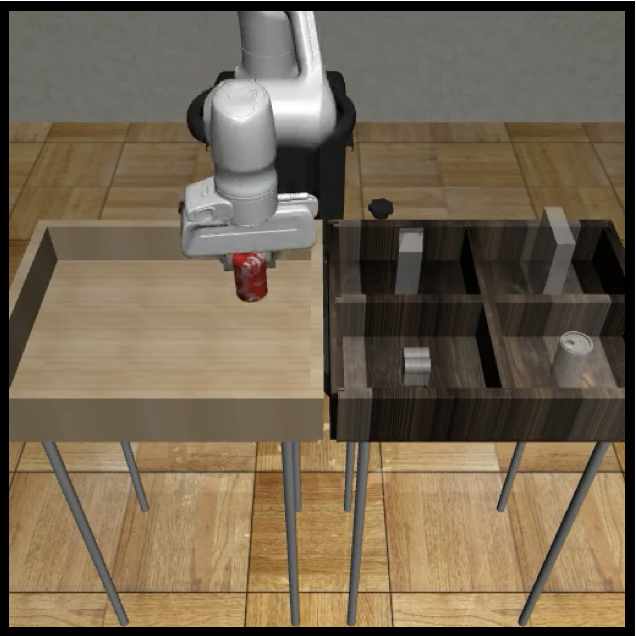
(a)

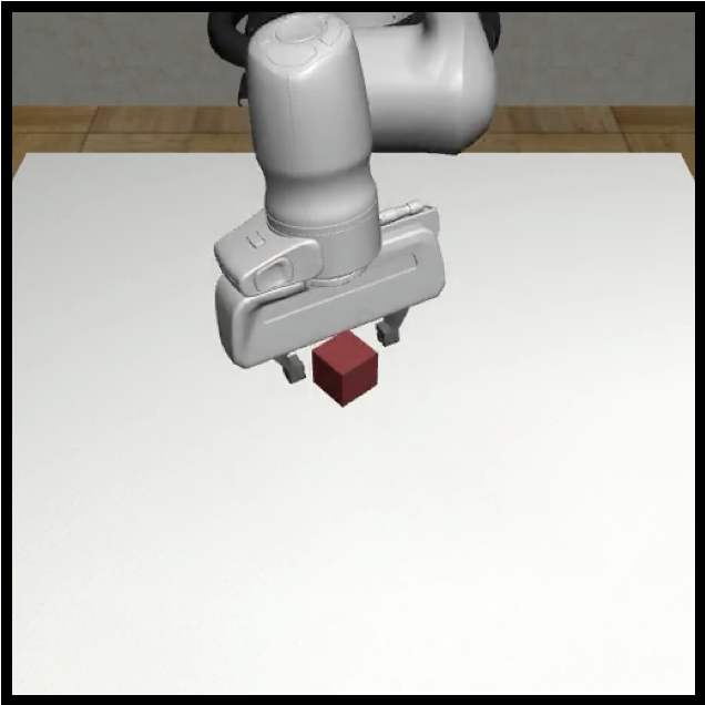
(b)

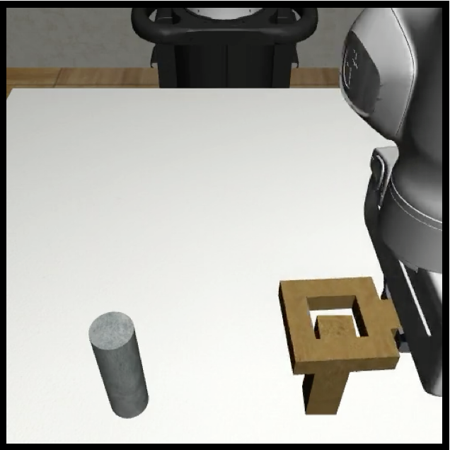
(c)

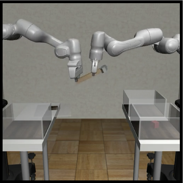
(d)

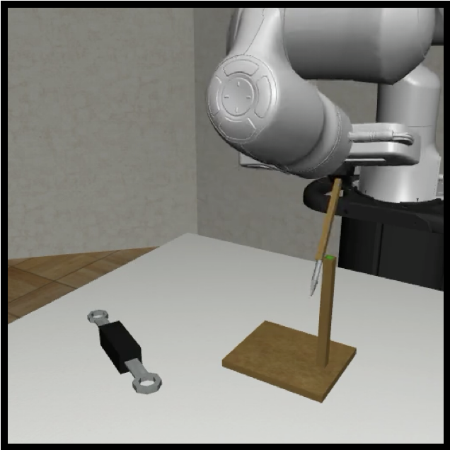
(e)

Figure 4: Visualizations of different tasks. (a) Can (b) Lift (c) Square (d) Transport (e) Tool_hang.

Fig. 4 illustrates the five subtasks in the RoboMimic Image dataset. Below we describe each subtask.

• Can (Fig. 4(a)): The robot must grasp a cylinder-shaped object and placing it into a bin. This subtask tests precise grasp planning and fingertip control under varying object poses Mandlekar et al. [2021].

• Lift (Fig. 4(b)): The manipulator picks up a heavier, irregularly shaped object (e.g. a small box) and raises it to a designated height. It evaluates the policy’s ability to modulate grip force and maintain stable trajectories Mandlekar et al. [2021].

• Square (Fig. 4(c)): The agent must push or slide an object so that its center follows a square-shaped path on the table. This challenges both straight-line control and precise cornering maneuvers Mandlekar et al. [2021].

• Transport (Fig. 4(d)): The agent must learn bimanual maneuvers to transfer a hammer from a closed container on a shelf to the target bin on another shelf. It tests coordinated lifting and translational motion under variable loads Mandlekar et al. [2021].

• Tool_Hang (Fig. 4(e)): The robot arm must learn high-precision manipulation behaviors to assemble a frame by inserting a hook into a narrow base. This requires fine-tuned wrist orientation and insertion accuracy Mandlekar et al. [2021].

A.2.2 Pre-trained Checkpoints

We use the pre-trained checkpoints of diffusion_policy_transformer model provided by Diffusion Policy Chi et al. [2023], where checkpoints of image-based tasks are stored under link and those of multi-stage tasks are stored under link. Following Diffusion Policy Chi et al. [2023], we evaluate the success rates of two types of checkpoints: The checkpoints that achieve the maximum performance during training and those stored in the last 10 epochs. For robustness, these checkpoints are collected in three training seeds.

A.3 Additional Experiments on $k$

In this experiment, we aim to answer two questions: (1) how $k$ influences the effectiveness of BUA in mitigating update-induced error? (2) Does the effectiveness of $k$ relate to $S$?

To answer question 1, we evaluate all tasks with $k=3$ and cache number $S=10$. As shown in Table 3, when $k=3$, the average success rates for the three task categories were 0.71, 0.77, and 0.97, respectively, which are slightly lower than those for $k=5$ (0.79, 0.77, 0.98) but still significantly better than the Uniform baseline. Increasing $k$ can further improve performance at the cost of higher computational overhead. Therefore, we choose $k=5$ as the default setting, as it achieves lossless performance while maximizing acceleration.

To answer question 2, we investigate the relationship between the hyperparameter $k$ (number of selected upstream blocks) and $S$ (cache number) in the context of the effectiveness of BUA in mitigating update-induced errors. The experimental results in Table 4 demonstrate that the effectiveness of $k$ is closely tied to $S$.

$k$ plays a more important role in mitigating update-induced errors. For certain difficult tasks, such as Tool_hang_ph and Transport_mh, the results for $k=3,S=20$ (e.g., 0.32/0.53 and 0.29/0.43, respectively) are outperformed by $k=5,S=10$ (e.g., 0.49/0.55 and 0.30/0.46, respectively). This indicates that an appropriately tuned $k$ plays a dominant role in optimizing the effectiveness of BUA for challenging tasks.

Notebly, the effectiveness of $k$ depends on an appropriate $S$. for a fixed $k=3$, increasing $S$ from 5 to 20 significantly improves the average success rate across tasks with performance collapse, from 0.07 at $S=5$ to 0.80 at $S=20$, suggesting that a larger number of cache update steps helps to mitigate update-induced errors. Thus, the interplay between $k$ and $S$ suggests that a balanced combination, such as $k=5,S=10$, achieves robust performance across diverse tasks.

Table 3: Effect of the hyperparameter $k$ on the mitigation of update-induced error across PH, MH and multi-stage settings by BUA ($S=10$).

Benchmark on Proficient Human (PH) demonstration data.

Method	Success Rate $\uparrow$						AVG	FLOPs	Speed $\times$
	Lift	Can	Square	Transport	Tool	Push–T
BAC(k=3)	1.00/1.00	0.93/0.96	0.83/0.91	0.81/0.79	0.03/0.07	0.59/0.60	0.71	2.39G	3.21
BAC(k=5)	1.00/1.00	0.94/0.97	0.82/0.89	0.77/0.82	0.49/0.55	0.59/0.62	0.79	2.66G	3.40

Benchmark on Mixed Human (MH) demonstration data.

Method	Success Rate $\uparrow$				AVG	FLOPs	Speed $\times$
	Lift	Can	Square	Transport
BAC(k=3)	0.97/0.99	0.93/0.97	0.79/0.77	0.21/0.53	0.77	2.48G	3.21
BAC(k=5)	0.99/0.98	0.95/0.97	0.77/0.79	0.30/0.46	0.77	2.64G	3.41

Benchmark on multi-stage tasks. For Block-Pushing, p_x is the frequency of pushing x blocks into the targets. For Kitchen, p_x is the frequency of interacting with x or more objects (e.g., bottom burner).

Method	Success Rate $\uparrow$						AVG	FLOPs	Speed $\times$
	BPp1	BPp2	Kitp1	Kitp2	Kitp3	Kitp4
BAC(k=3)	0.99/0.98	0.94/0.93	0.99/1.00	0.97/0.99	0.95/0.99	0.89/0.97	0.97	2.23G	3.38
BAC(k=5)	1.00/0.99	0.97/0.95	1.00/0.99	1.00/0.99	1.00/0.99	0.94/0.97	0.98	2.44G	3.60

Table 4: Benchmark Results across tasks that have performance collapse (Tool_hang_ph, Transport_mh, Kitchen), all results set $k=3$ and $S\in\{5,7,20\}$.

Method	Success Rate $\uparrow$						AVG	FLOPs	Speed $\times$
	Toolph	Transmh	Kitp1	Kitp2	Kitp3	Kitp4
BAC (S=5)	0.00/0.00	0.26/0.50	0.04/0.07	0.00/0.00	0.00/0.00	0.00/0.00	0.07	1.49G	4.02
BAC (S=7)	0.00/0.01	0.19/0.32	0.82/0.93	0.64/0.79	0.55/0.70	0.33/0.52	0.49	1.90G	3.66
BAC (S=10)	0.03/0.07	0.21/0.53	0.99/1.00	0.97/0.99	0.95/0.99	0.89/0.97	0.72	2.43G	3.34
BAC (S=20)	0.32/0.53	0.29/0.43	1.00/1.00	1.00/1.00	1.00/1.00	0.99/0.97	0.80	4.16G	2.53

A.4 Additional Experiments on Different Similarity Metrics

In this experiment, we evaluate the performance of BAC across all tasks using four similarity metrics: Mean Squared Error (MSE), Lorm-1 distance (L1), Wasserstein-1 distance (Wa), and Cosine similarity (Cosine), as presented in Table 5. BAC with metric Cosine achieves average success rates of 0.79, 0.77, and 0.98 for PH, MH, and multi-stage tasks, outperforming BAC with metric MSE (0.78, 0.70, 0.98), BAC with metric L1 (0.72, 0.67, 0.98) and BAC with metric Wa (0.70, 0.56, 0.81). BAC with metric Cosine excels particularly in MH settings while matching MSE and L1 in multi-stage tasks. BAC with metric Wa struggles with complex tasks (e.g., Kit_p4: 0.39/0.67). All metrics exhibit similar computational costs, with FLOPs ranging from 2.40G to 2.73G and speed from 3.07$\times$ to 3.42$\times$. Thus, BAC with metric Cosine and BAC with metric MSE demonstrate the most robust performance, with Cosine preferred for noisy data and complex tasks.

Table 5: Benchmark Results across Proficient Human (PH), Mixed Human (MH), and Multi-stage Demonstrations ($k=5$, $S=10$) using MSE, L1 and Wa Metrics.

Benchmark on Proficient Human (PH) demonstration data.

Method	Success Rate $\uparrow$						AVG	FLOPs	Speed $\times$
	Lift	Can	Square	Transport	Tool	Push–T
BAC(MSE)	1.00/1.00	0.79/0.79	0.71/0.83	0.75/0.77	0.40/0.55	0.58/0.66	0.78	2.73G	3.21
BAC(L1)	1.00/1.00	0.89/0.95	0.74/0.85	0.71/0.73	0.19/0.33	0.56/0.65	0.72	2.60G	3.19
BAC(Wa)	1.00/1.00	0.37/0.75	0.79/0.87	0.80/0.79	0.37/0.50	0.52/0.61	0.70	2.73G	3.28
BAC(Cosine)	1.00/1.00	0.94/0.97	0.82/0.89	0.77/0.82	0.49/0.55	0.59/0.62	0.79	2.66G	3.40

Benchmark on Mixed Human (MH) demonstration data.

Method	Success Rate $\uparrow$				AVG	FLOPs	Speed $\times$
	Lift	Can	Square	Transport
BAC(MSE)	1.00/0.99	0.41/0.86	0.75/0.77	0.26/0.50	0.70	2.69G	3.21
BAC(L1)	0.97/1.00	0.44/0.87	0.71/0.74	0.23/0.43	0.67	2.63G	3.18
BAC(Wa)	0.98/0.99	0.83/0.90	0.09/0.05	0.19/0.45	0.56	2.71G	3.07
BAC(Cosine)	0.99/0.98	0.95/0.97	0.77/0.79	0.30/0.46	0.77	2.64G	3.41

Benchmark on multi-stage tasks. For Block-Pushing, p_x is the frequency of pushing x blocks into the targets. For Kitchen, p_x is the frequency of interacting with x or more objects (e.g., bottom burner).

Method	Success Rate $\uparrow$						AVG	FLOPs	Speed $\times$
	BPp1	BPp2	Kitp1	Kitp2	Kitp3	Kitp4
BAC(MSE)	0.99/0.99	0.95/0.93	1.00/1.00	1.00/1.00	0.99/0.99	0.97/0.93	0.98	2.49G	3.39
BAC(L1)	0.99/0.99	0.94/0.94	1.00/1.00	1.00/1.00	1.00/1.00	0.93/0.95	0.98	2.40G	3.42
BAC(Wa)	0.99/1.00	0.95/0.95	0.83/0.95	0.66/0.90	0.55/0.85	0.39/0.67	0.81	2.61G	3.08
BAC(Cosine)	1.00/0.99	0.97/0.95	1.00/0.99	1.00/0.99	1.00/0.99	0.94/0.97	0.98	2.44G	3.60

A.5 More details on Temporal Similarities

We compute cosine similarity between intermediate features of different timesteps to analyze temporal similarity patterns, using the Square_ph task as a case study. Fig. 6 provides more details on the temporal similarity patterns of different decoder blocks. The observation that the feature similarity between consecutive timesteps varies non-uniformly over time exists in all the decoder blocks. This suggests the necessity of our ACS.

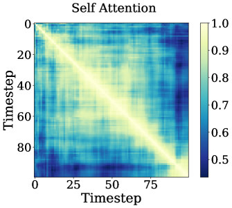
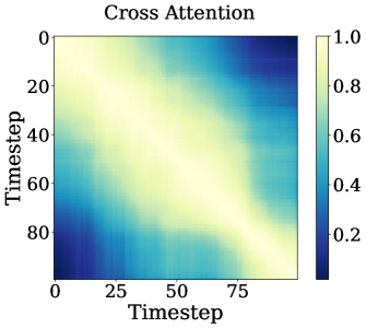
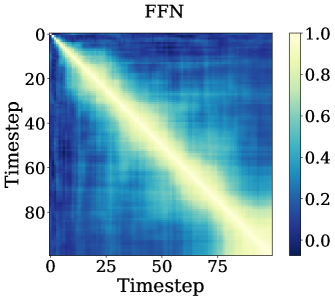
(a) Feature similarities across timesteps in the first layer.

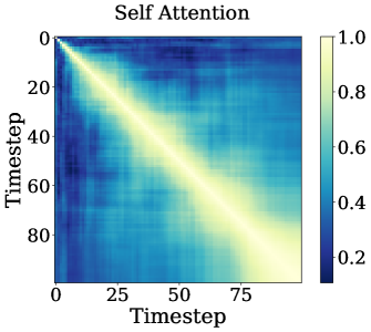
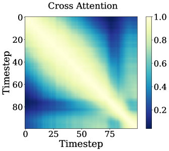
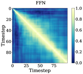
(b) Feature similarities across timesteps in the second layer.

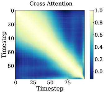
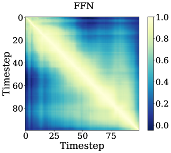
(c) Feature similarities across timesteps in the third layer.

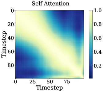
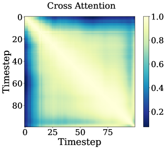
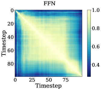
(d) Feature similarities across timesteps in the fourth layer.

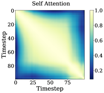
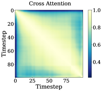
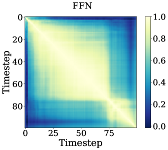
(a) Feature similarities across timesteps in the fifth layer.

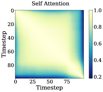
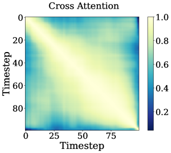
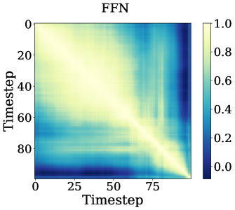
(b) Feature similarities across timesteps in the sixth layer.

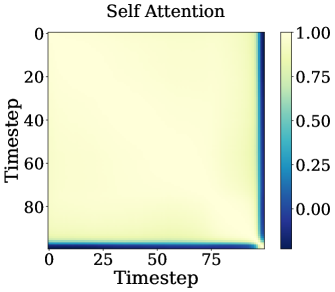
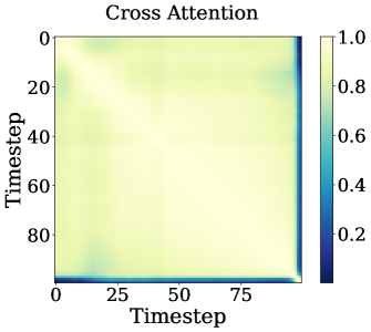
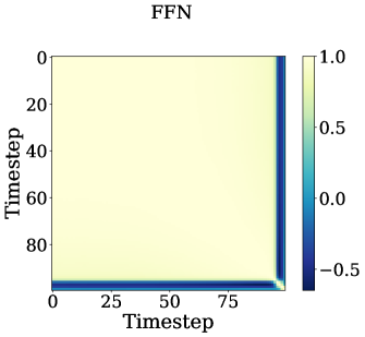
(c) Feature similarities across timesteps in the seventh layer.

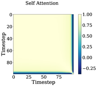
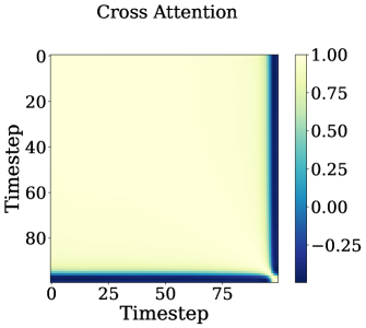
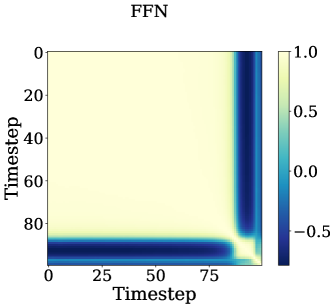
(d) Feature similarities across timesteps in the eighth layer.

Figure 6: Feature similarities across timesteps for different blocks in each decoder layer.

To provide more details on the block-wise temporal similarity pattern, we compute cosine similarities under different intervals of consecutive steps in timestep $t$ and earlier timesteps $t{-}k$ for various values of $k$ (1, 5, 10, 15, 20). As shown in Fig. 7, different blocks exhibit distinct temporal similarity patterns. Some blocks maintain high similarity across long horizons, indicating few updates, while others show rapid drops in similarity even at short intervals, suggesting more update steps. This suggests the necessity of a block-wise schedule.

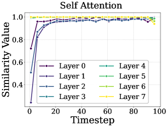
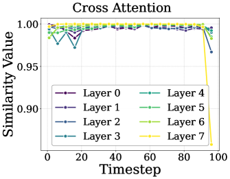
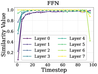
(a) Similarity change curves, measured between timestep $t$ and $t{-}1$.

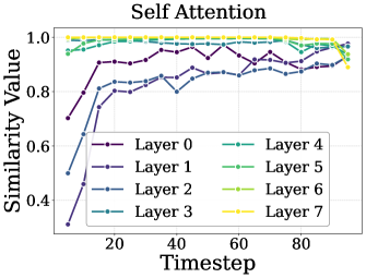
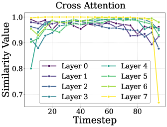
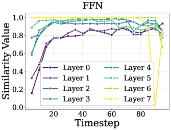
(b) Similarity change curves, measured between timestep $t$ and $t{-}5$.

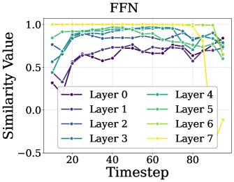
(c) Similarity change curves, measured between timestep $t$ and $t{-}10$.

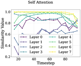
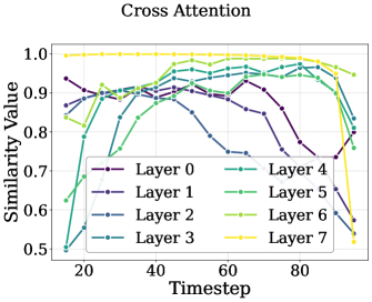
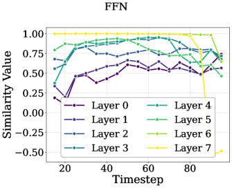
(d) Similarity change curves, measured between timestep $t$ and $t{-}15$.

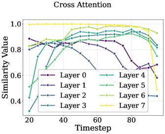
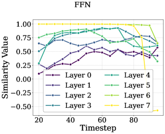
(e) Similarity change curves, measured between timestep $t$ and $t{-}20$.

Figure 7: Block-wise feature similarity between consecutive steps. Each subfigure shows the similarity between features at timestep $t$ and ($t{-}k$, where $k=1,5,10,15,20$) for different blocks.

A.6 More details on the high episode homogeneity within individual tasks

In this section, we present evidence for the high episode homogeneity of an embodied task by highlighting the distinct similarity patterns in action generation tasks versus image generation tasks.

In action generation tasks, as shown in Fig. 9, we visualize the feature similarity matrices from the same layer of Diffusion Policy, under the same task (Square_ph), across two different scene demos (demo id 11001 vs. demo id 20000). Despite changes in scene settings, the similarity matrices remain strikingly consistent, suggesting a high degree of representational homogeneity across episodes.

In contrast, in image generation tasks, as shown in Fig. 10, we visualize the feature similarity matrices from the same layer of DiT-XL/2 Peebles and Xie [2023], across two different classes in ImageNet (class label 15: "robin, American robin, Turdus migratorius" vs. class label 800: "slot, one-armed bandit"). The results from both the self-attention and MLP blocks reveal clear differences in feature patterns.

While an image generation task shows obvious differences in feature patterns across different classes, an action generation task shows almost no difference across different scene demos within the same task. These observations support the efficiency of our method, specifically in embodied episodes. Benefiting from the high episode homogeneity within individual tasks, our method can be run only once for a given task before inference, incurring virtually no additional cost.

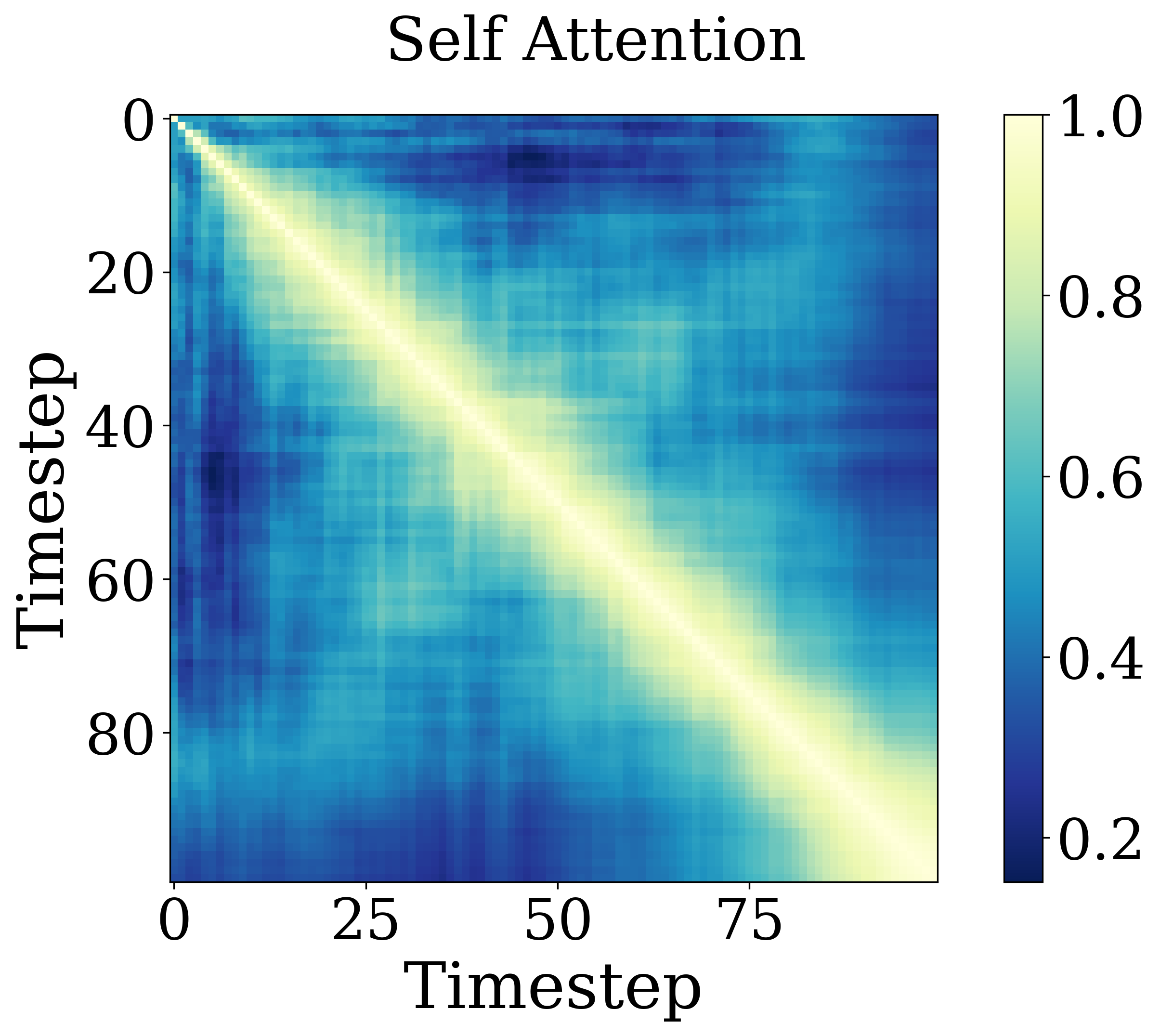
(a) Diffusion Policy demo 11001.

(b) Diffusion Policy demo 20000.

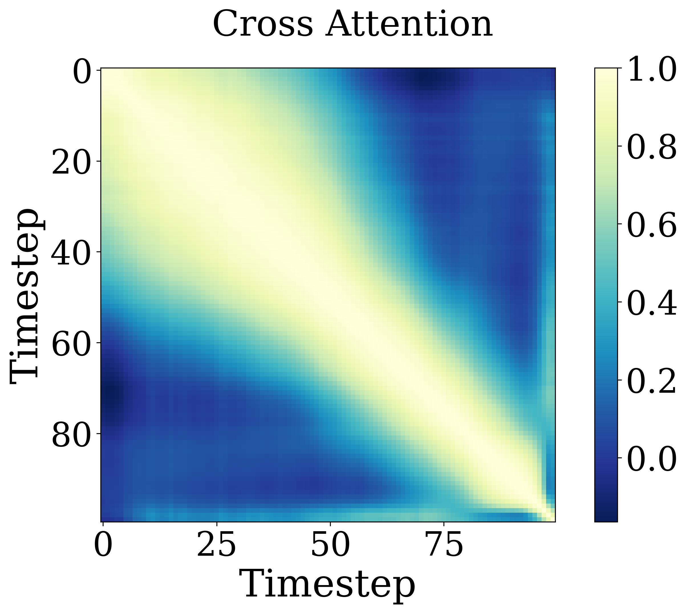
(c) Diffusion Policy demo 11001.

(d) Diffusion Policy demo 20000.

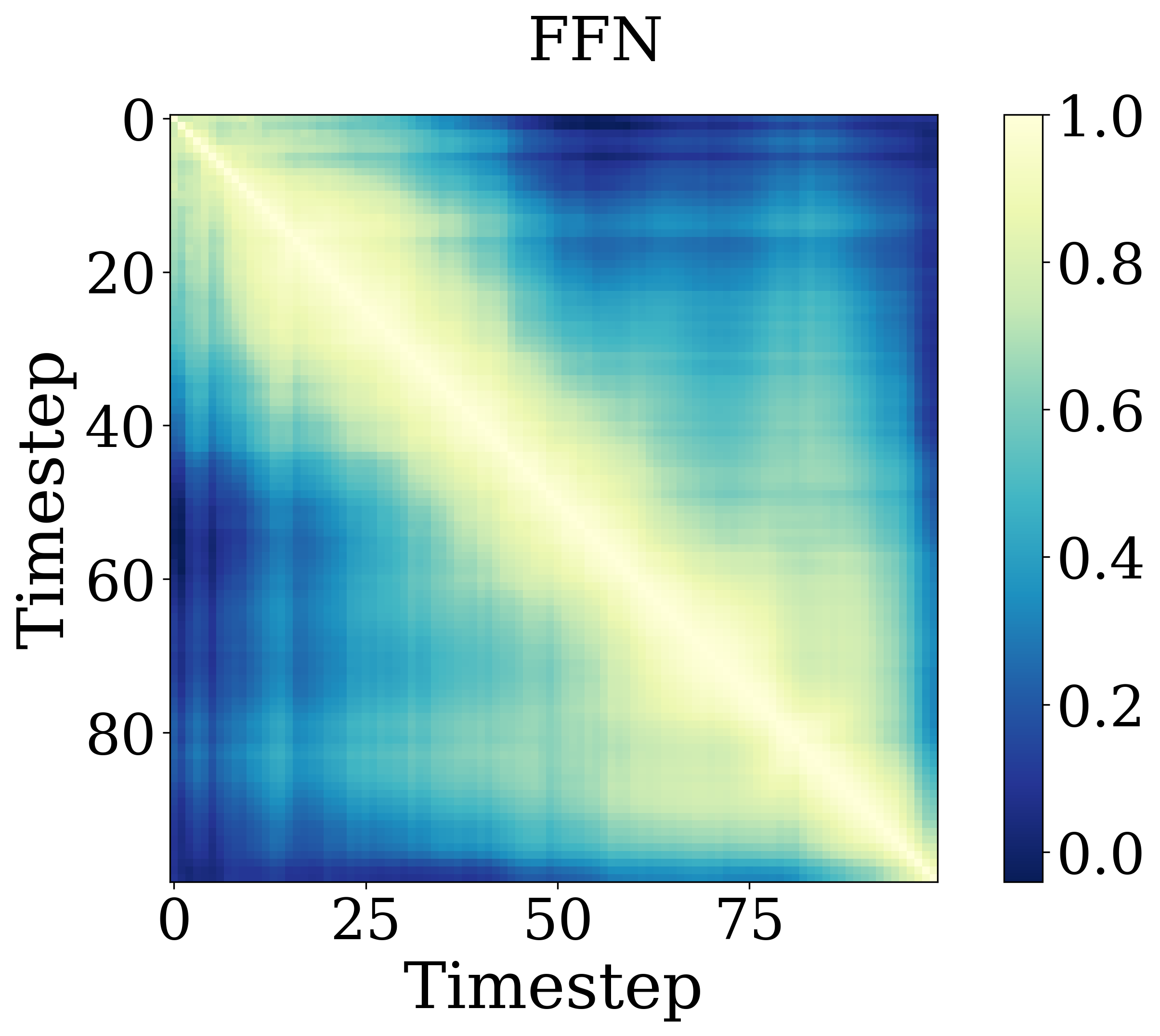
(e) Diffusion Policy demo 11001.

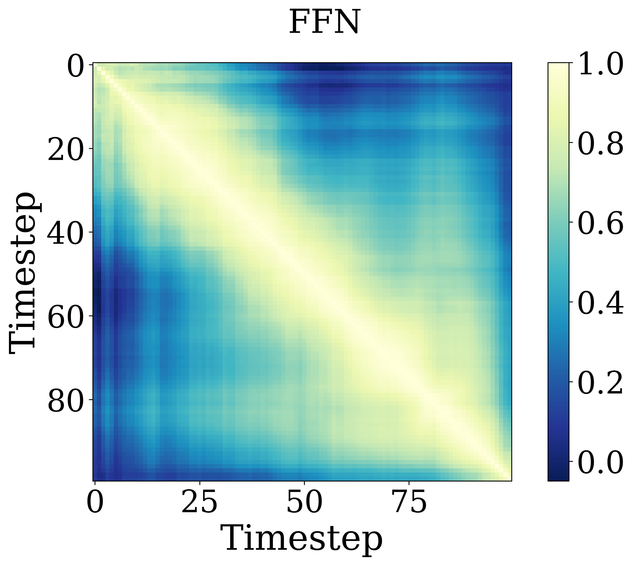
(f) Diffusion Policy demo 20000.

.

Figure 9: Feature similarities across timesteps in action generation tasks. We visualize similarity matrices of different blocks in the third layer across different scene demos (e.g., demo id 11001 vs. demo id 20000).

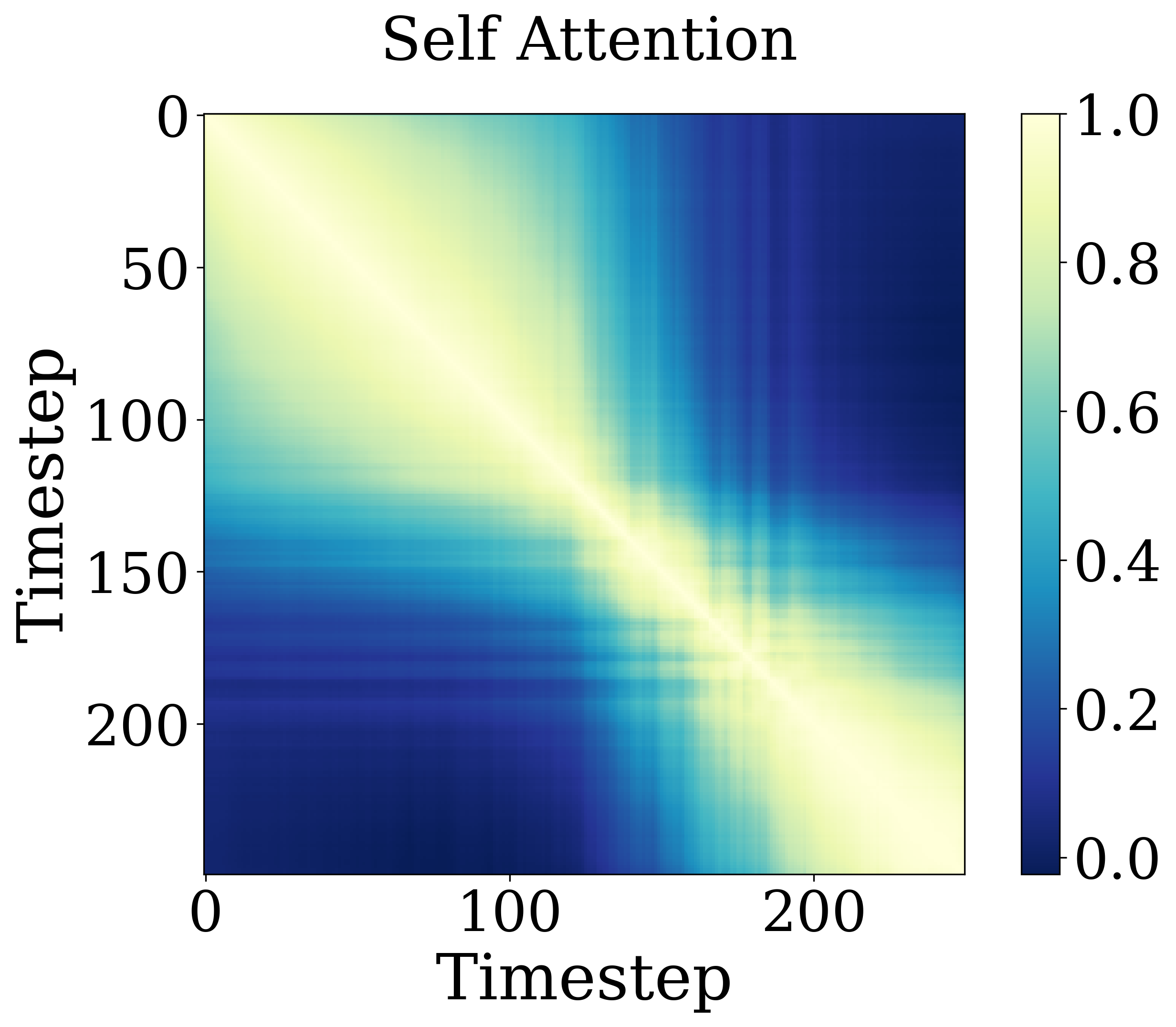
(a) Diffusion Model class label 15.

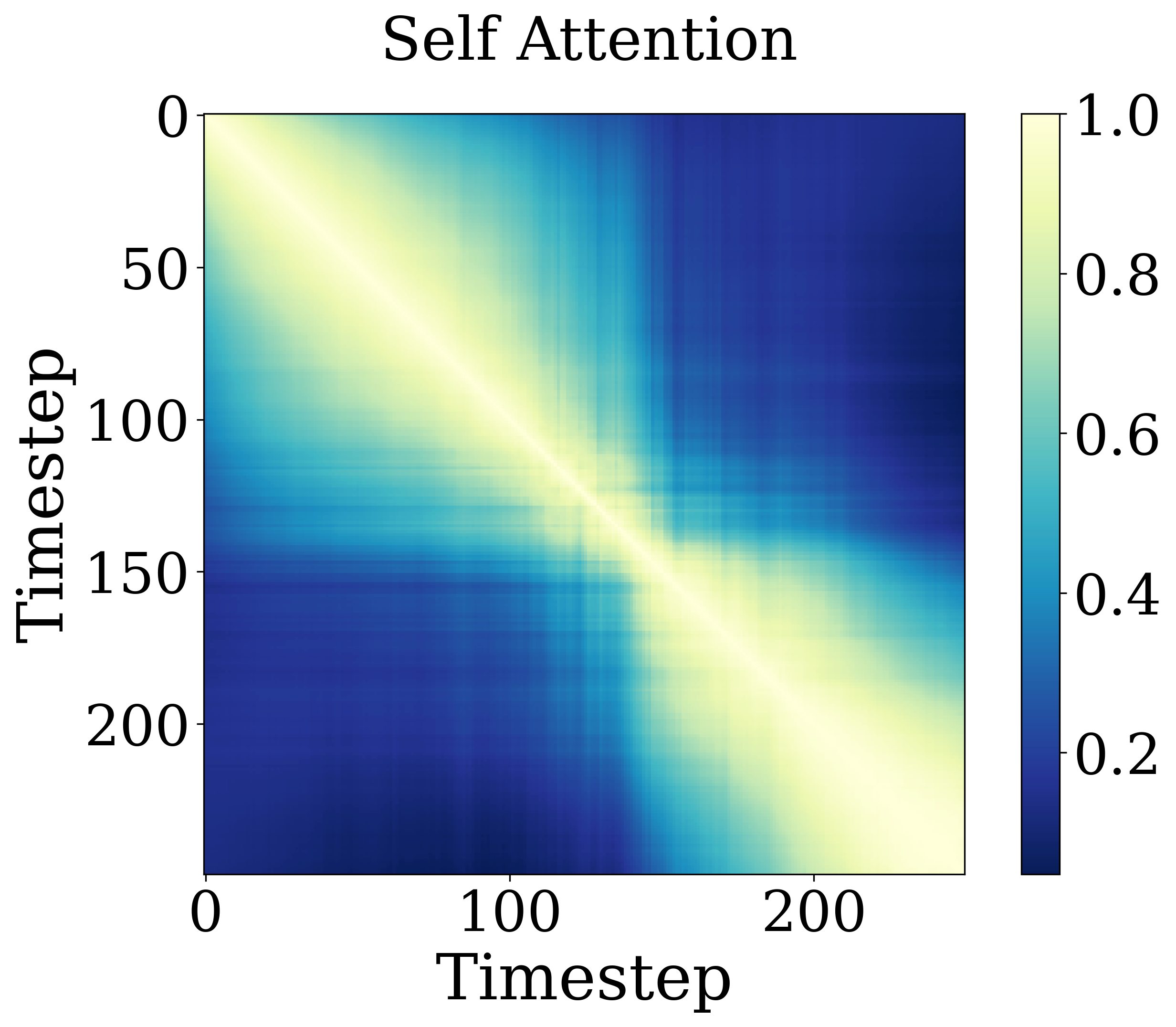
(b) Diffusion Model class label 800.

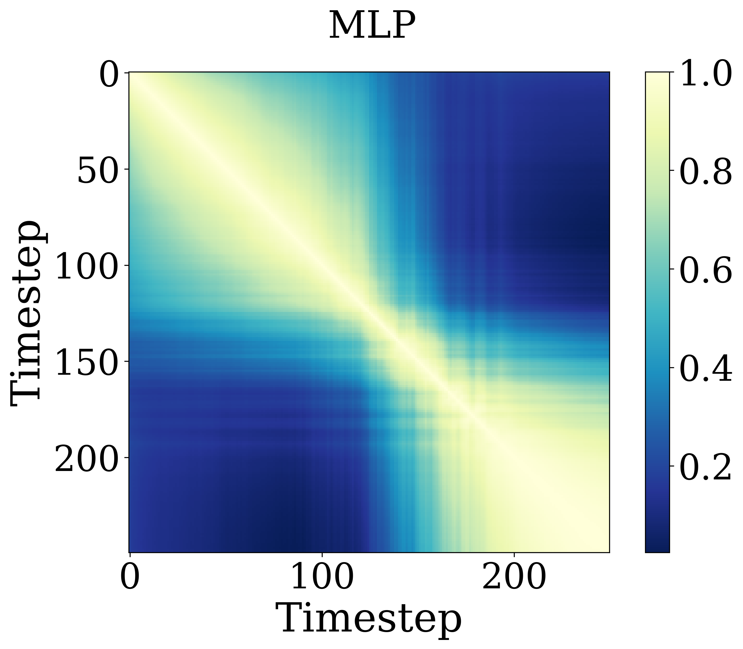
(c) Diffusion Model class label 15.

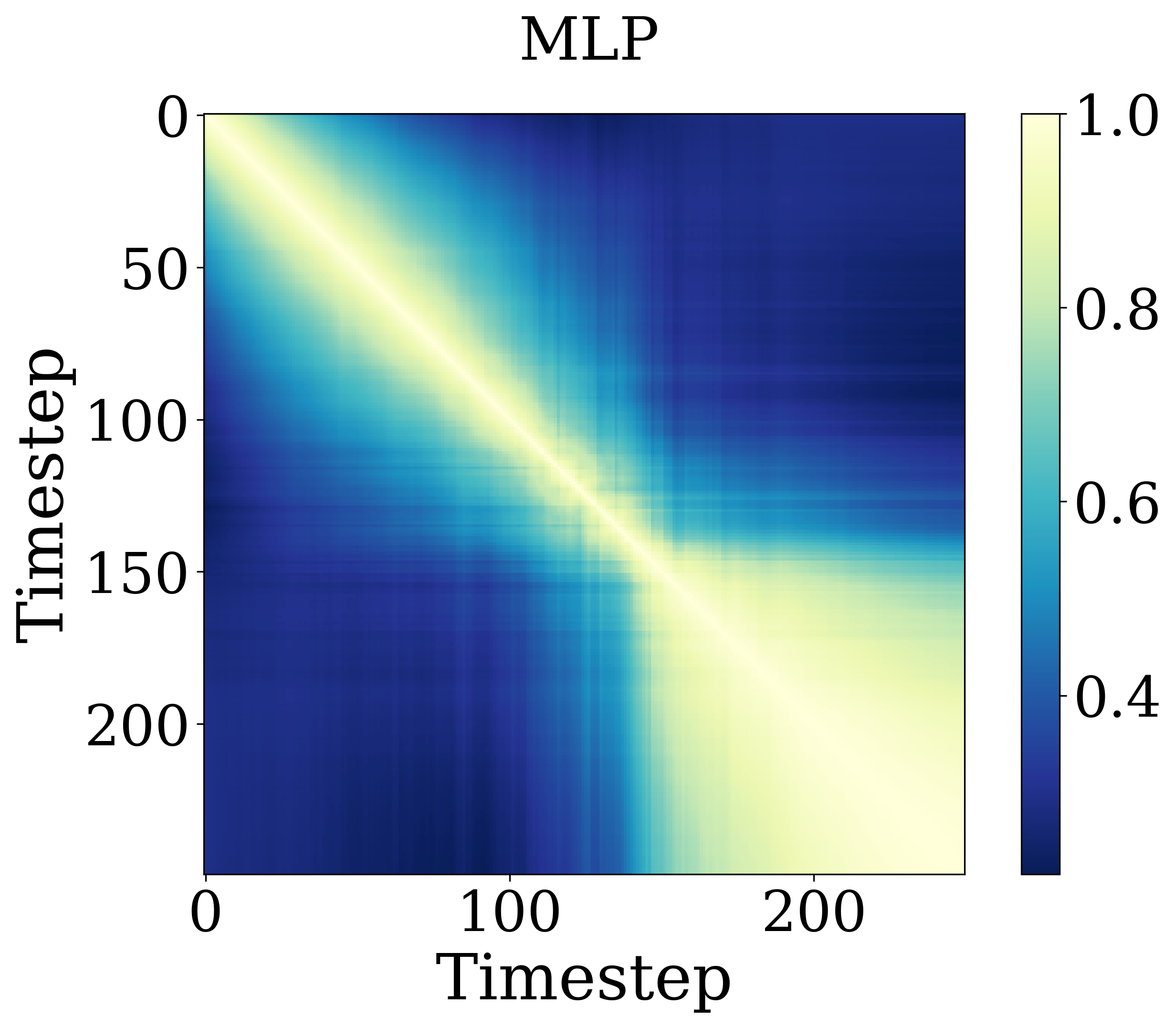
(d) Diffusion Model class label 800.

Figure 10: Feature similarities across timesteps in image generation tasks. We visualize similarity matrices of different blocks in the fourteenth layer across different classes (e.g., class label 15 vs. class label 800).

A.7 More details for Fig.3

To support findings of the error surge phenomenon, we present comparisons of caching errors across different FFN blocks using a block-wise schedule versus a unified schedule. As shown in Fig. 12, the block-wise schedule leads to error surges in nearly all FFN blocks except the first one, in contrast to the unified schedule. This observation further suggests that caching errors can propagate through downstream FFN blocks.

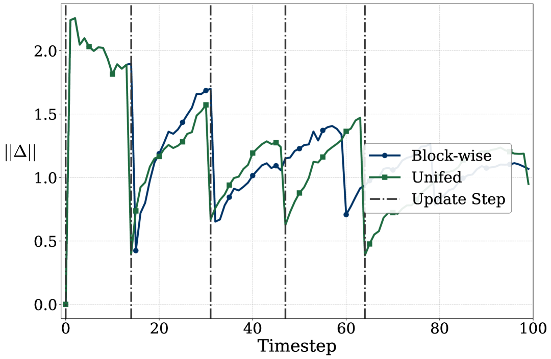
(a) Caching error in the first FFN block.

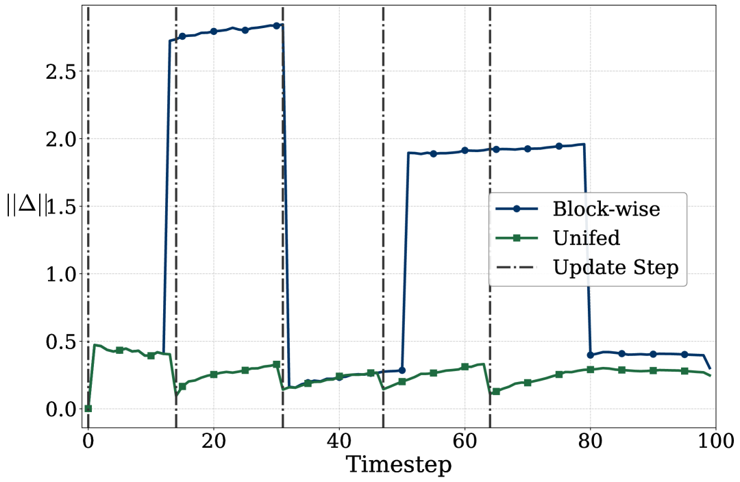
(b) Caching error in the second FFN block.

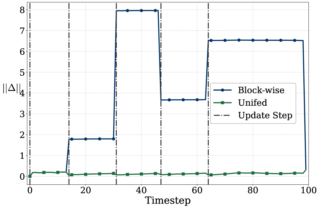
(a) Caching error in the third FFN block.

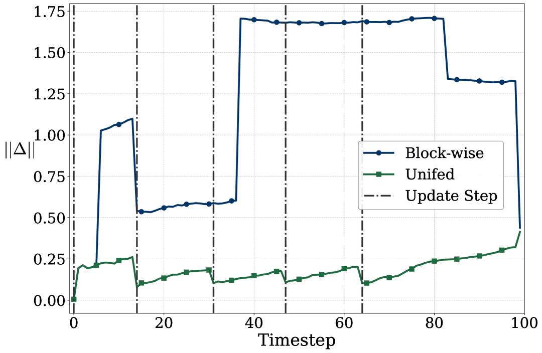
(b) Caching error in the fourth FFN block.

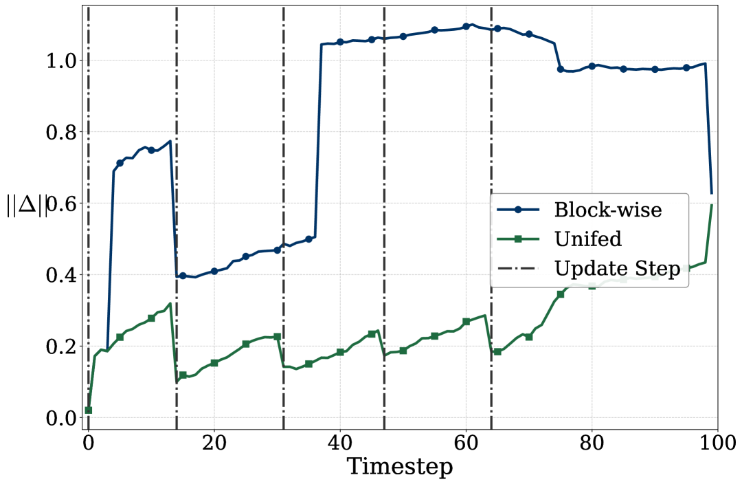
(c) Caching error in the fifth FFN block.

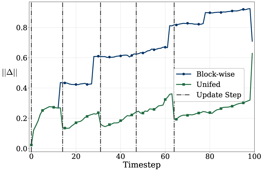
(d) Caching error in the sixth FFN block.

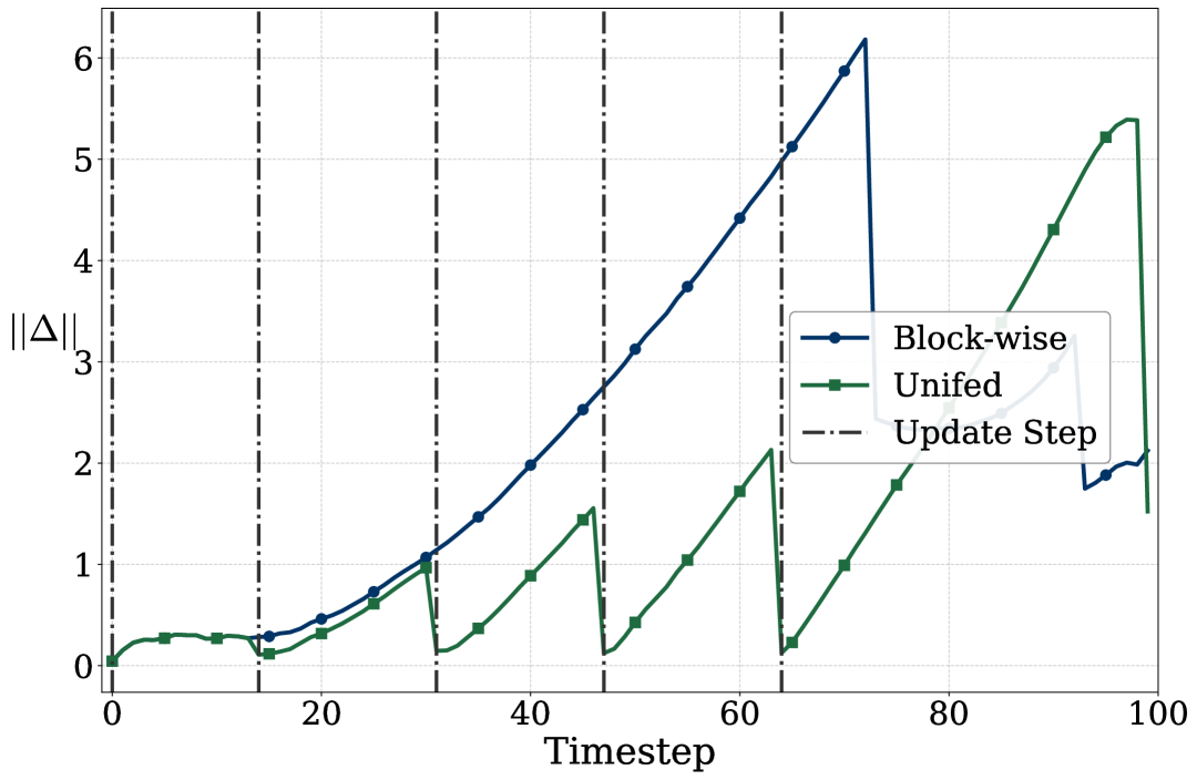
(e) Caching error in the seventh FFN block.

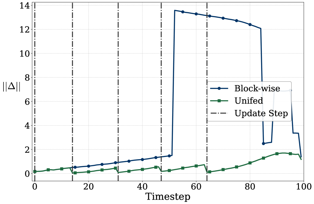
(f) Caching error in the eighth FFN block.

Figure 12: Caching error across different FFN blocks using a block-wise schedule versus a unified one.

Fig. 14 presents block-wise heatmaps of caching error across all blocks throughout the diffusion process, covering a diverse set of tasks and two demonstration settings: Proficient Human (PH) and Mixed Human (MH). Each subfigure corresponds to a different task, with color intensity representing the magnitude of caching error at each block and timestep, and white dots indicating cache update steps.

These visualizations support our analysis of inter-block error propagation by consistently exhibiting the following key phenomenon: in multiple tasks, blocks occasionally update at steps where their upstream blocks with large caching errors have not yet been updated. This mismatch leads to sudden, sharp increases in error (seen as abrupt darkening) in the downstream block, with no smooth transition. Importantly, even after upstream blocks are later updated, the downstream surge in error remains, indicating that the update failed to recover from the propagated upstream error.

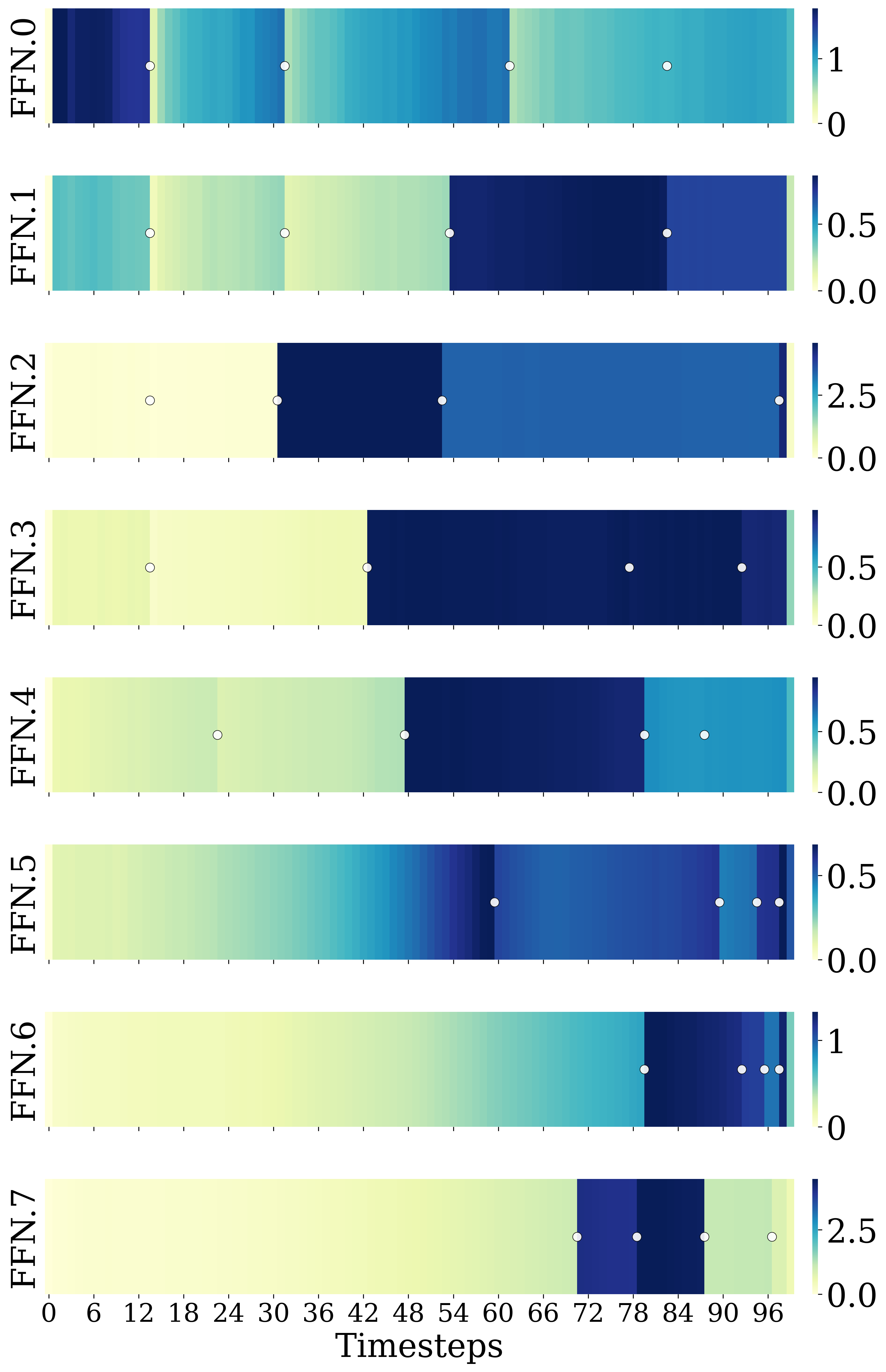
(a) Can_mh

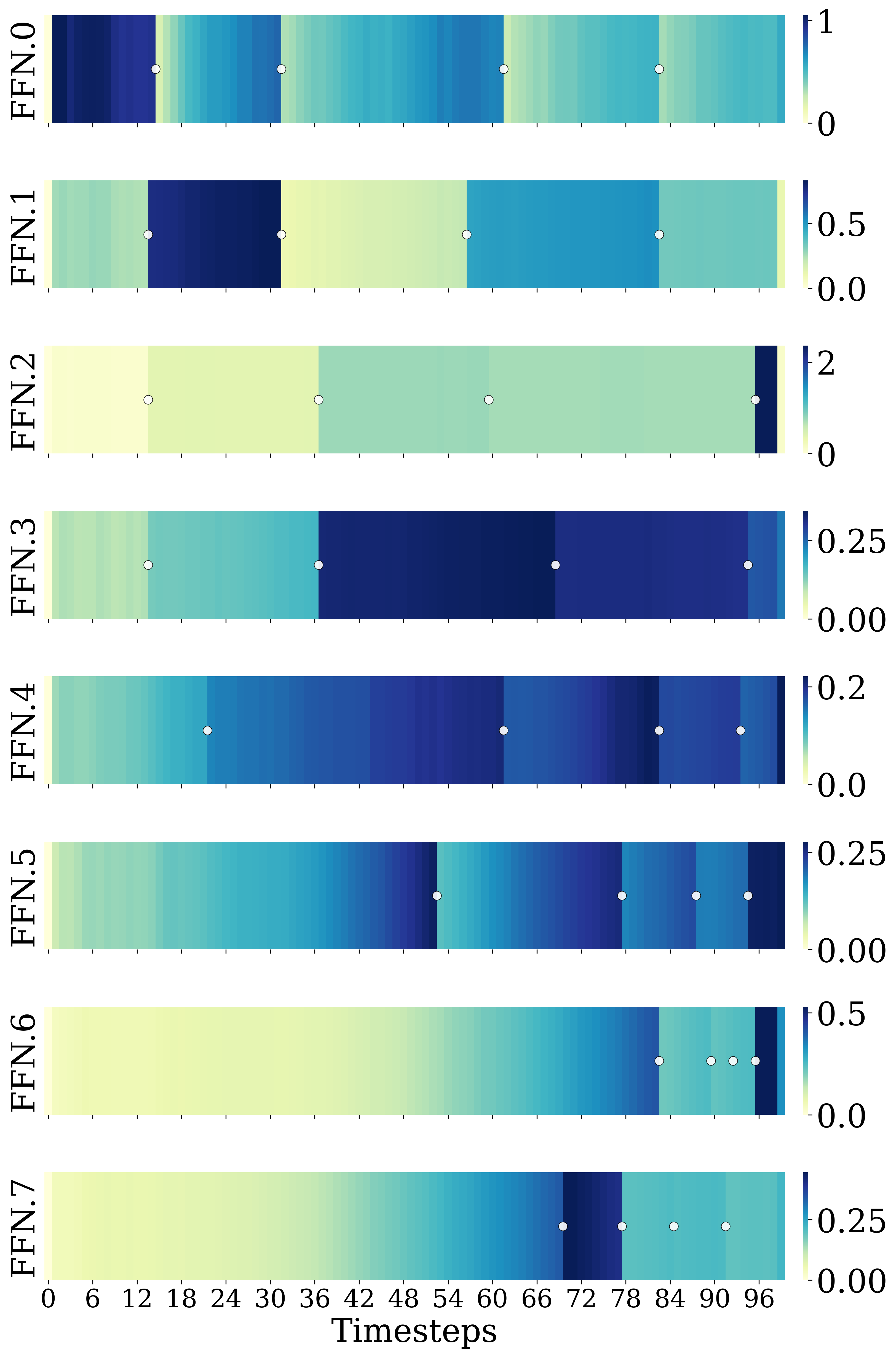
(b) Can_ph

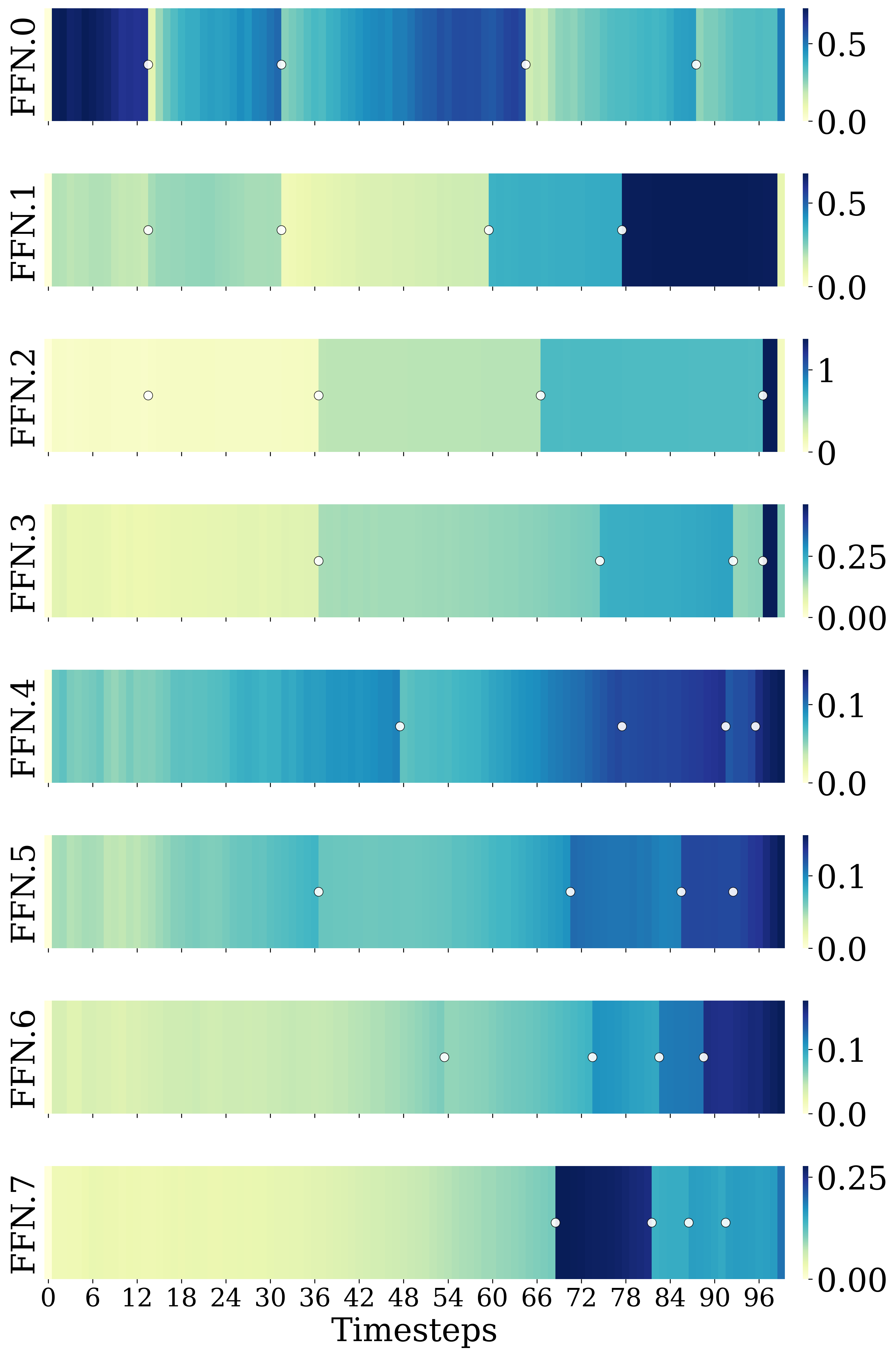
(c) Lift_mh

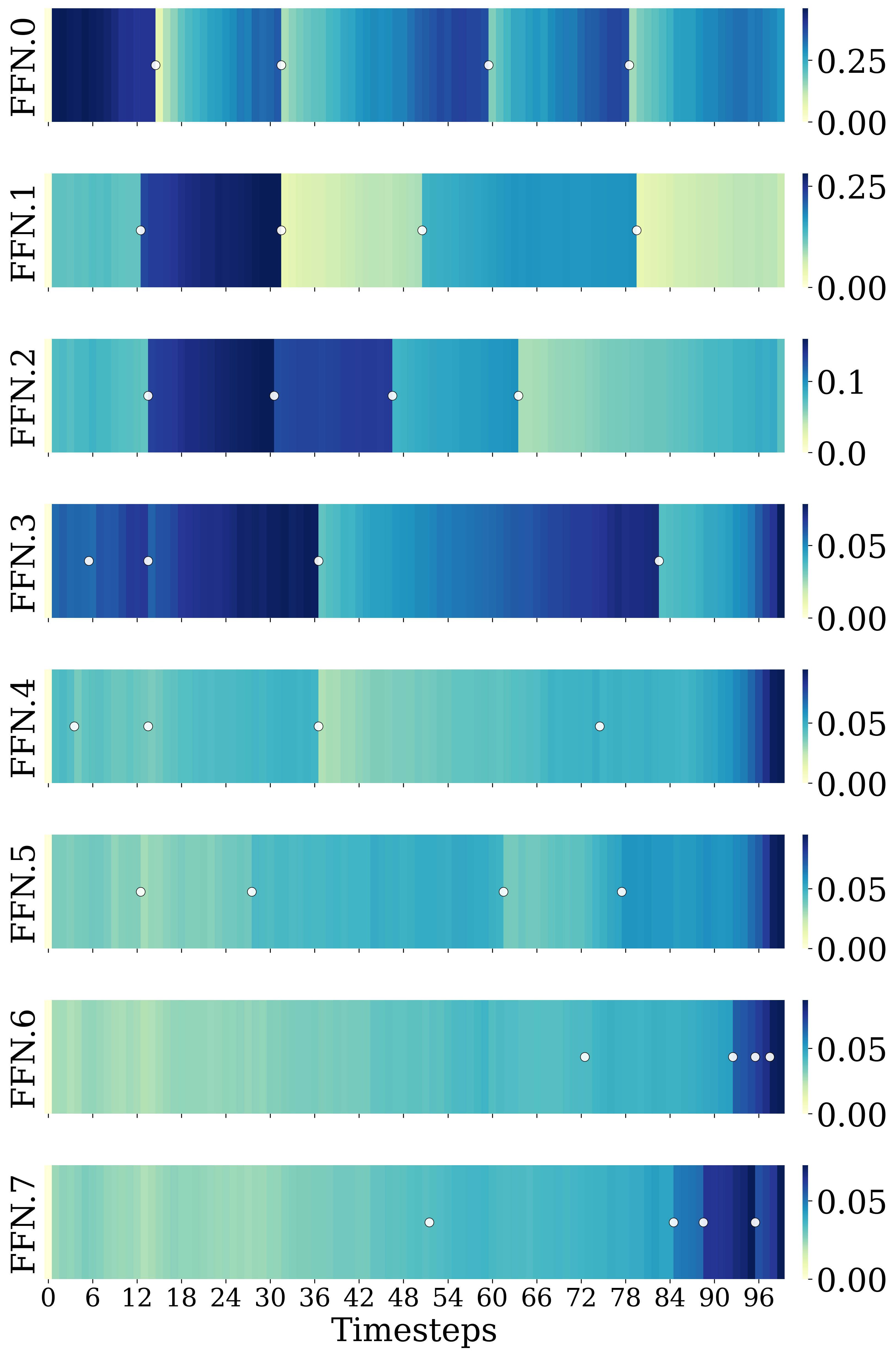
(d) Lift_ph

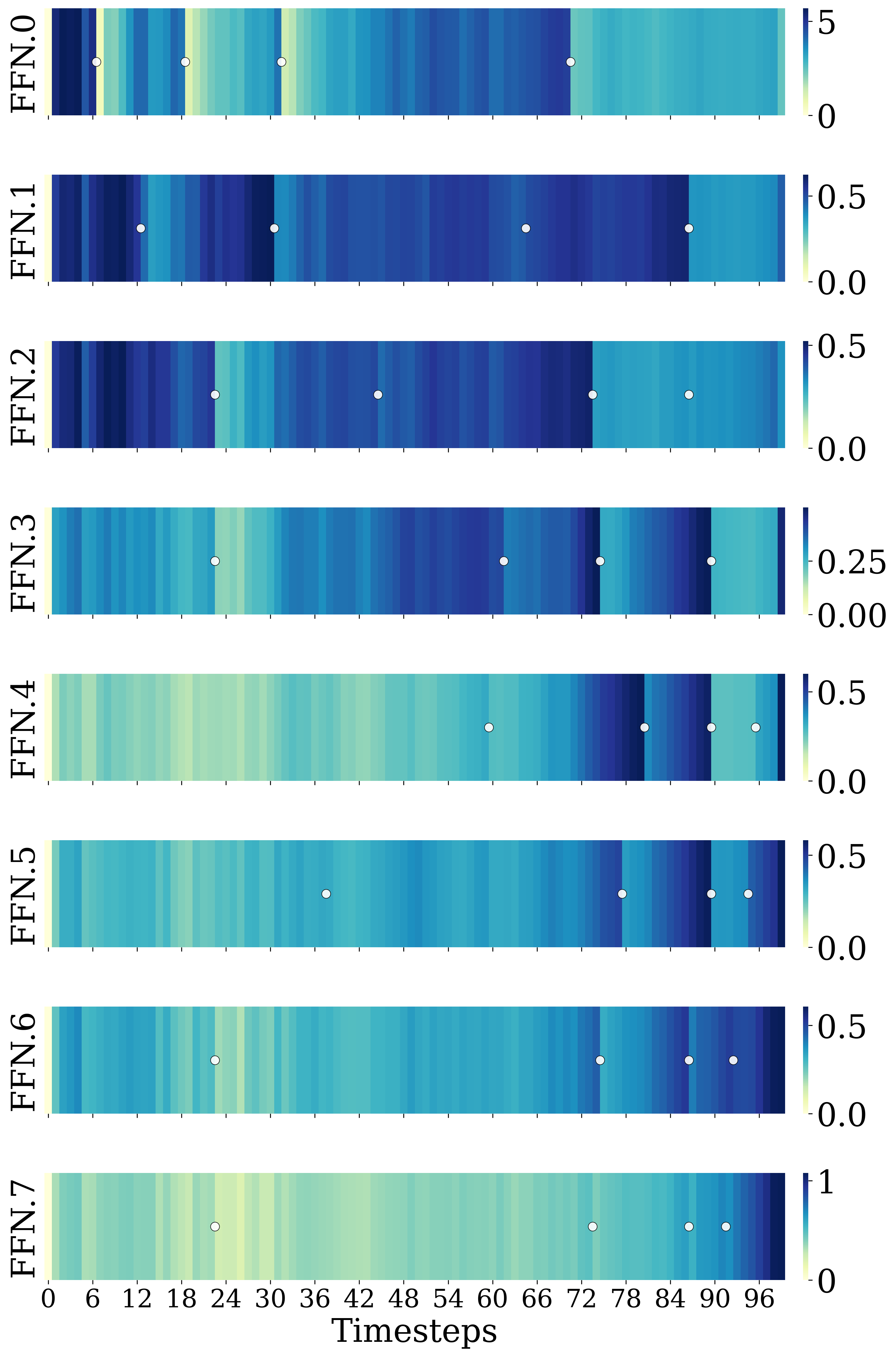
(e) Push-T_ph

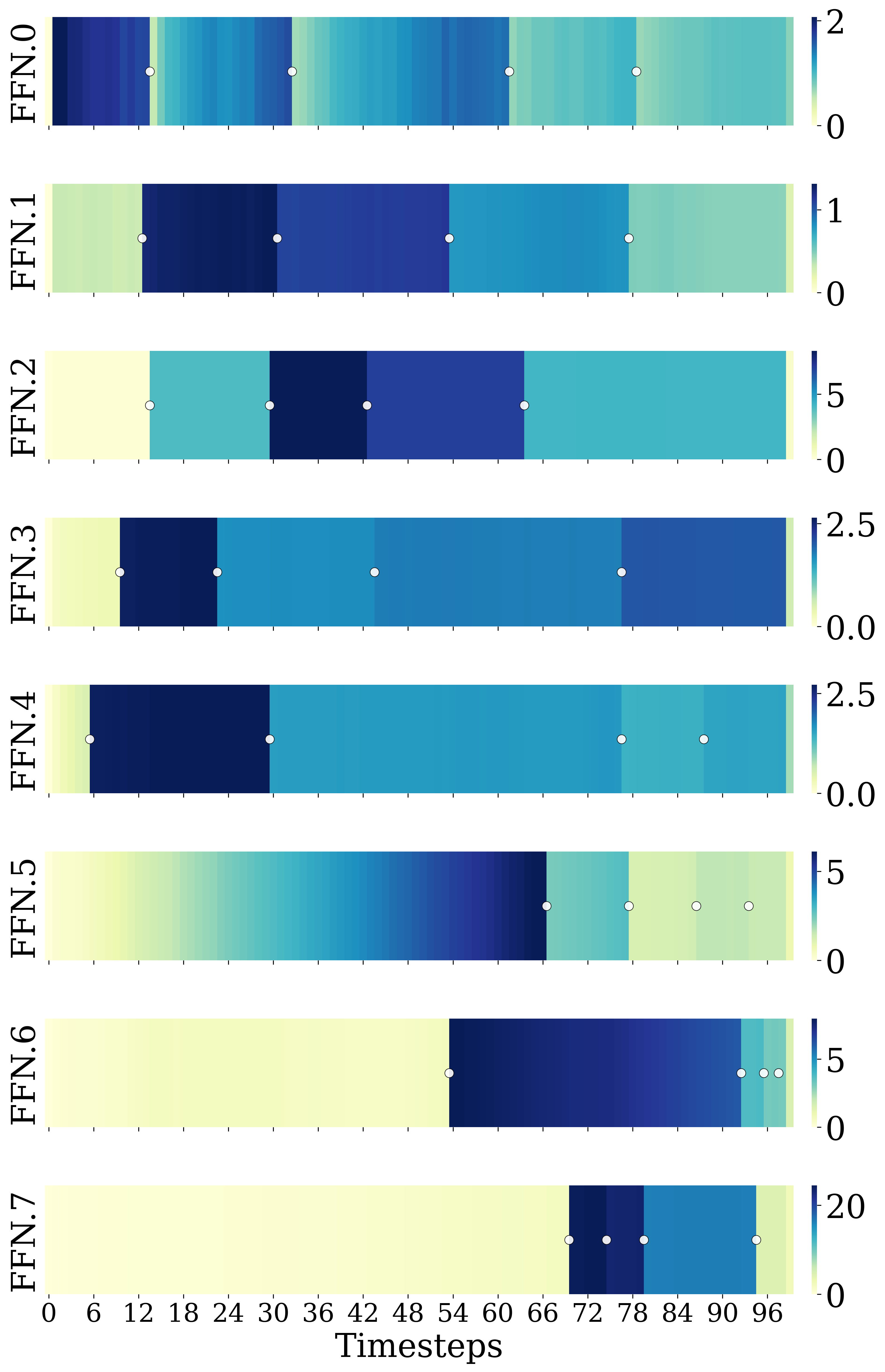
(f) Square_mh

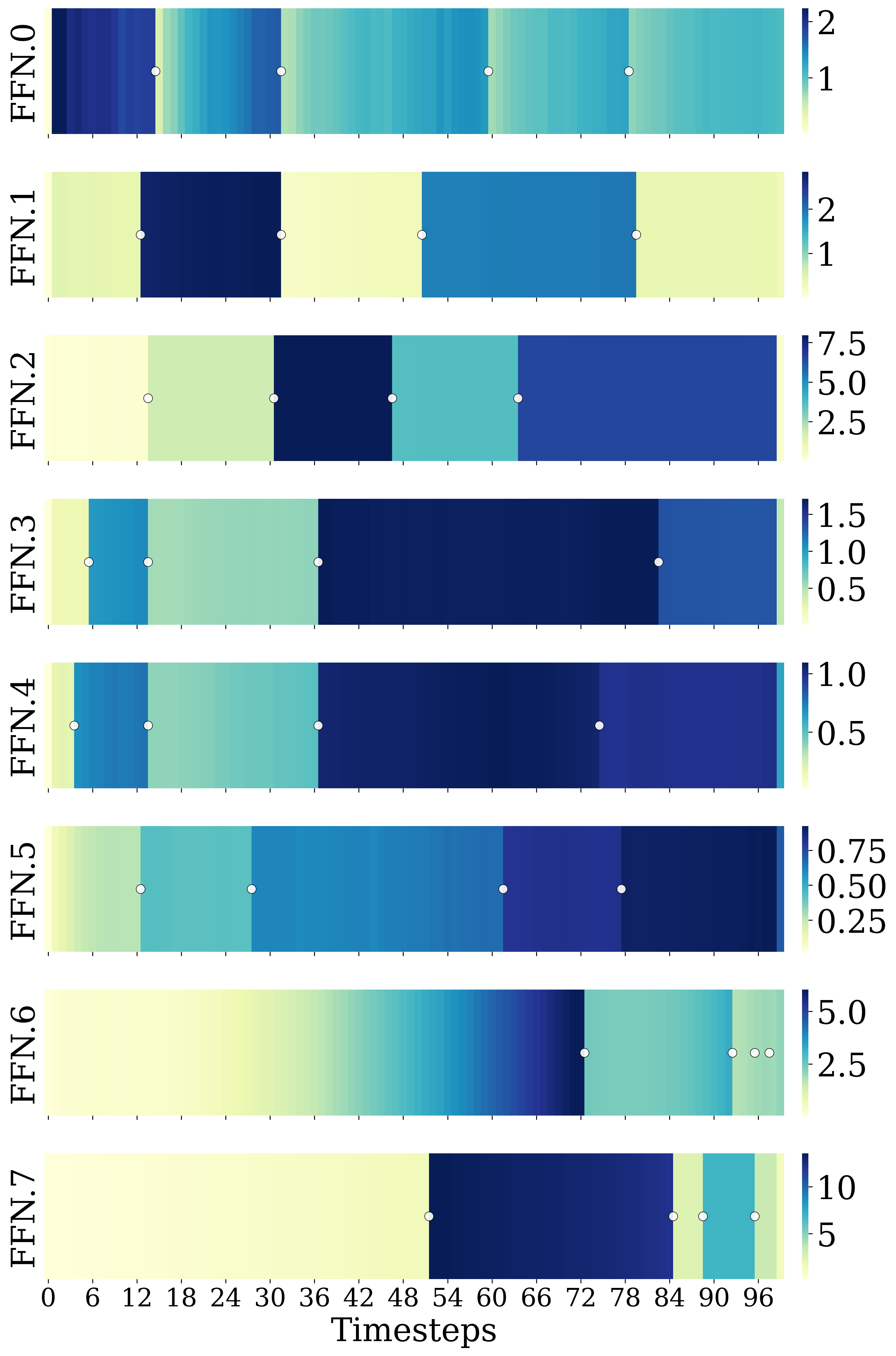
(g) Square_ph

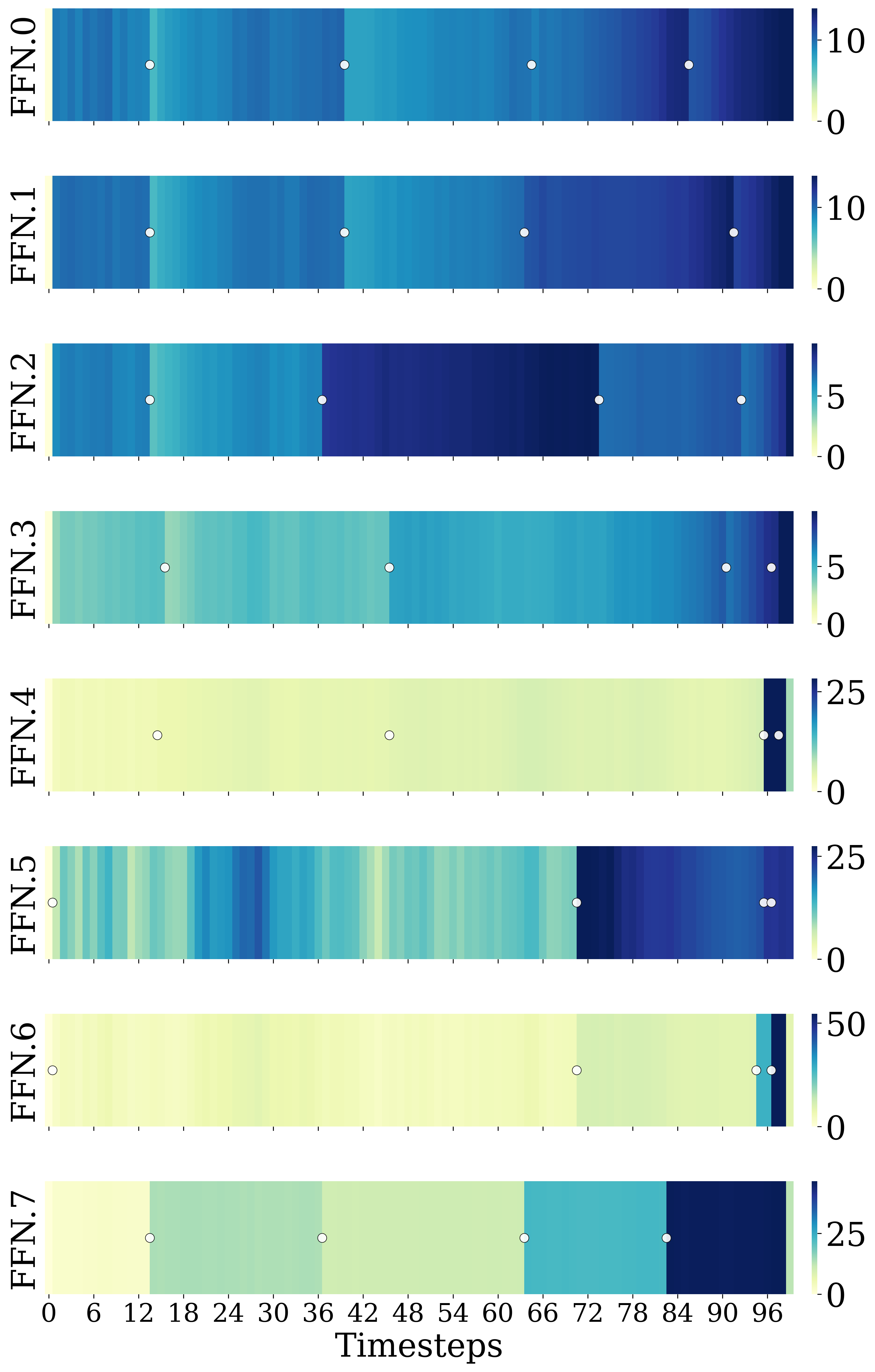
(h) Transport_mh

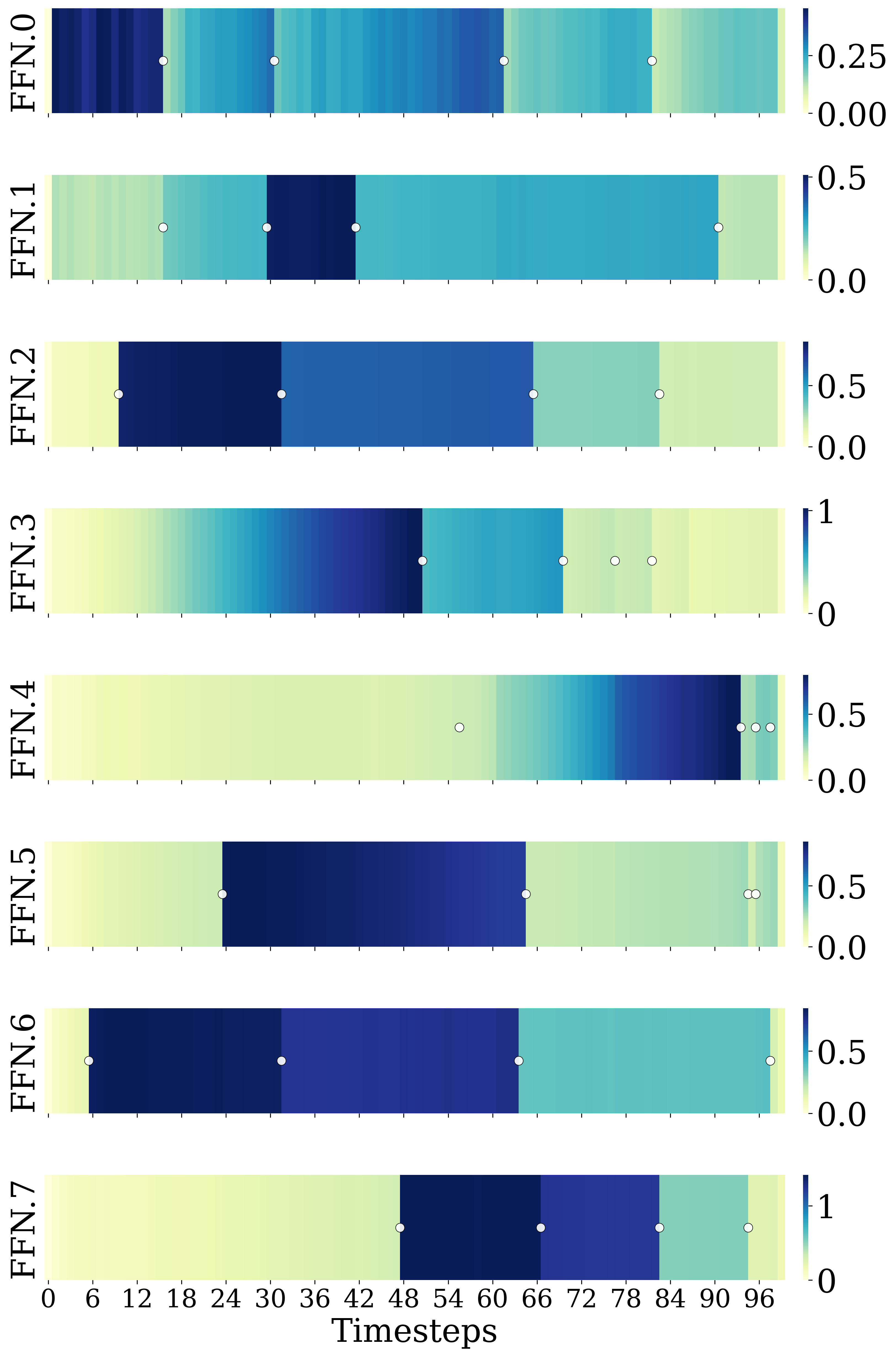
(i) Transport_ph

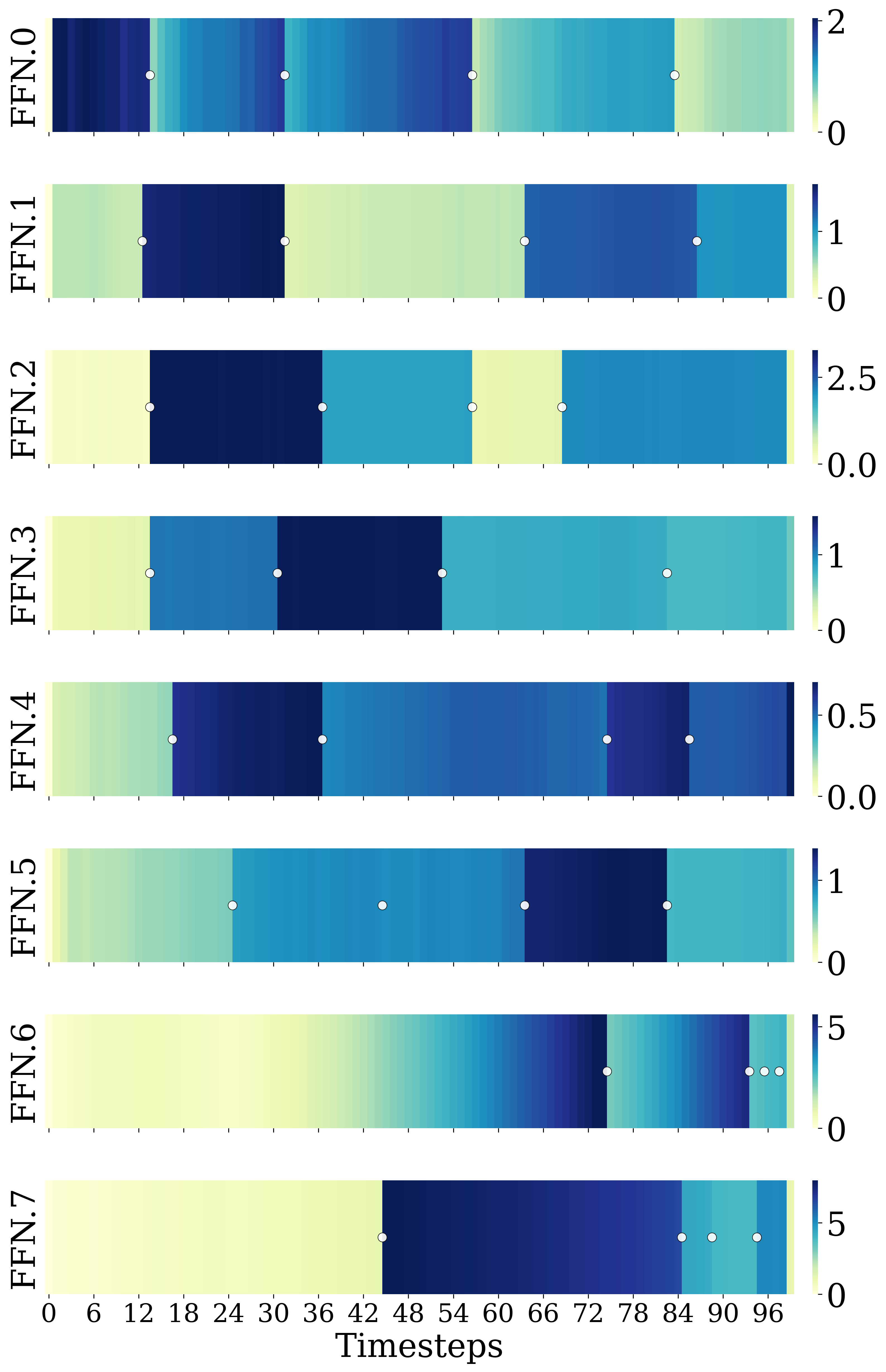
(a) Tool_hang_ph

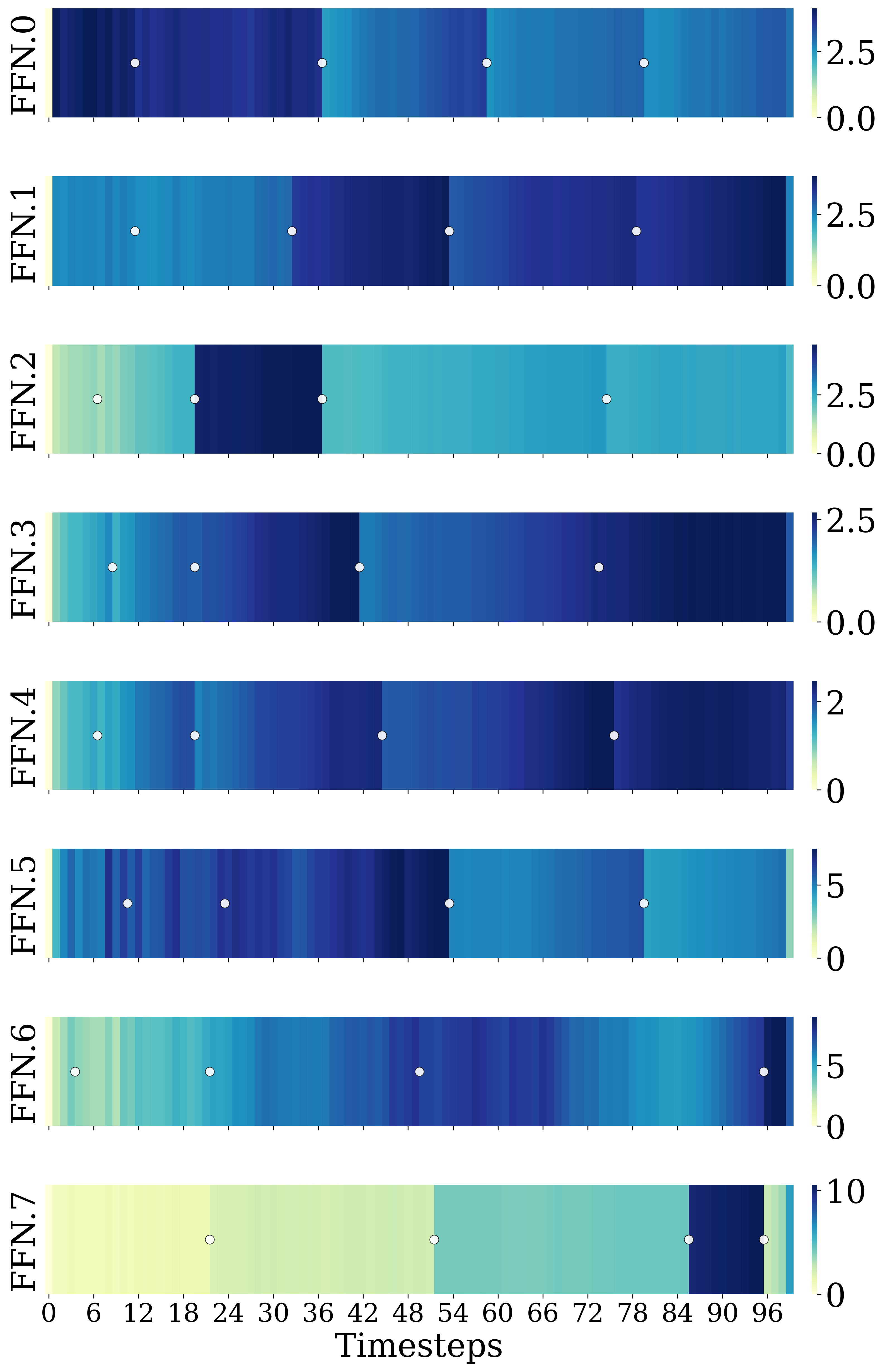
(b) Kitchen

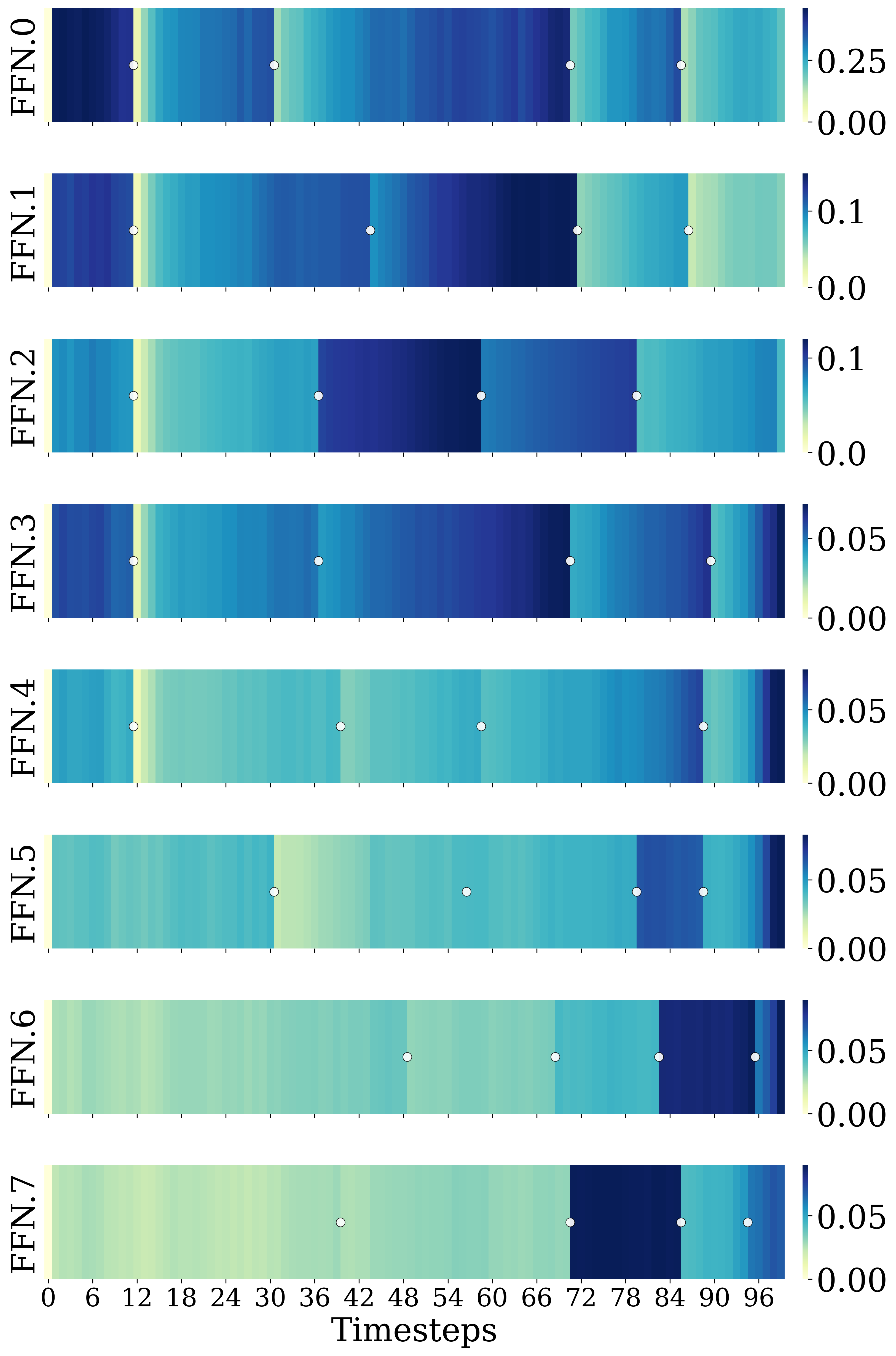
(c) Block Pushing

Figure 14: Caching error across all blocks throughout the diffusion process, with white dots indicating update steps.

A.8 Details on Update Steps Computed by ACS

Our algorithm employs a two-stage paradigm where we apply ACS followed by BUA to determine the optimal update steps for different blocks in the offline stage, and then accelerate Diffusion Policy by updating and reusing the cached features based on the prepared update steps in the online stage.

In Tables 6,7,8,9,10,11,12,13,14,15,16 and 17, we report the update steps after employing ACS for all blocks across all tasks at $S=10$.

Table 6: Update steps for Can_ph computed by ACS.

Block	Steps
layers.0.SA	0, 2, 9, 18, 30, 49, 62, 69, 82, 91
layers.0.CA	0, 18, 33, 44, 57, 71, 80, 84, 89, 94
layers.0.FFN	0, 4, 10, 19, 31, 40, 53, 65, 79, 88
layers.1.SA	0, 4, 10, 21, 32, 44, 54, 65, 79, 88
layers.1.CA	0, 14, 25, 36, 48, 60, 73, 82, 87, 93
layers.1.FFN	0, 8, 16, 28, 38, 51, 60, 68, 80, 93
layers.2.SA	0, 4, 8, 13, 28, 38, 54, 68, 80, 90
layers.2.CA	0, 9, 18, 28, 38, 51, 67, 80, 86, 95
layers.2.FFN	0, 14, 27, 37, 51, 62, 71, 80, 85, 95
layers.3.SA	0, 19, 30, 40, 51, 62, 72, 82, 90, 98
layers.3.CA	0, 6, 14, 25, 37, 49, 62, 75, 90, 98
layers.3.FFN	0, 4, 14, 23, 37, 48, 60, 78, 89, 95
layers.4.SA	0, 13, 25, 37, 53, 66, 81, 90, 95, 98
layers.4.CA	0, 3, 9, 22, 39, 57, 80, 86, 94, 98
layers.4.FFN	0, 6, 18, 39, 62, 75, 80, 86, 93, 96
layers.5.SA	0, 6, 22, 42, 63, 80, 88, 93, 96, 98
layers.5.CA	0, 4, 11, 29, 43, 61, 81, 90, 95, 98
layers.5.FFN	0, 37, 60, 79, 88, 92, 94, 96, 98, 99
layers.6.SA	0, 37, 67, 83, 89, 92, 94, 96, 97, 98
layers.6.CA	0, 13, 28, 51, 74, 88, 93, 95, 96, 98
layers.6.FFN	0, 28, 62, 80, 89, 93, 95, 96, 97, 99
layers.7.SA	0, 29, 64, 79, 86, 93, 95, 96, 97, 98
layers.7.CA	0, 12, 26, 49, 68, 83, 89, 93, 95, 97
layers.7.FFN	0, 47, 69, 74, 77, 81, 86, 95, 97, 99

Table 7: Update steps for Lift_ph computed by ACS.

Block	Steps
layers.0.SA	0, 1, 6, 51, 67, 76, 82, 87, 92, 95
layers.0.CA	0, 22, 44, 60, 70, 75, 80, 85, 93, 96
layers.0.FFN	0, 4, 8, 16, 27, 37, 49, 62, 74, 88
layers.1.SA	0, 4, 10, 19, 28, 37, 53, 65, 78, 88
layers.1.CA	0, 15, 26, 34, 39, 48, 60, 69, 78, 92
layers.1.FFN	0, 4, 10, 18, 28, 37, 54, 65, 79, 88
layers.2.SA	0, 2, 7, 19, 31, 40, 51, 63, 75, 87
layers.2.CA	0, 6, 22, 33, 39, 48, 68, 79, 90, 96
layers.2.FFN	0, 4, 10, 17, 27, 37, 51, 65, 78, 88
layers.3.SA	0, 6, 19, 40, 65, 74, 81, 86, 94, 98
layers.3.CA	0, 6, 15, 22, 38, 53, 66, 78, 88, 97
layers.3.FFN	0, 4, 14, 31, 49, 68, 79, 88, 93, 97
layers.4.SA	0, 6, 19, 40, 65, 75, 85, 92, 95, 98
layers.4.CA	0, 10, 21, 32, 44, 57, 70, 81, 90, 97
layers.4.FFN	0, 15, 37, 68, 79, 88, 93, 96, 98, 99
layers.5.SA	0, 19, 40, 65, 75, 81, 85, 89, 93, 96
layers.5.CA	0, 9, 18, 27, 37, 56, 62, 69, 76, 86
layers.5.FFN	0, 4, 15, 37, 48, 74, 88, 93, 96, 98
layers.6.SA	0, 7, 19, 40, 58, 67, 74, 84, 90, 96
layers.6.CA	0, 8, 15, 23, 34, 44, 54, 71, 87, 95
layers.6.FFN	0, 15, 31, 44, 57, 69, 79, 88, 93, 97
layers.7.SA	0, 7, 19, 39, 53, 67, 75, 84, 89, 96
layers.7.CA	0, 8, 14, 23, 35, 45, 57, 71, 81, 95
layers.7.FFN	0, 15, 29, 40, 54, 69, 79, 86, 91, 95

Table 8: Update steps for Square_ph computed by ACS.

Block	Steps
layers.0.SA	0, 3, 9, 17, 30, 49, 62, 69, 80, 89
layers.0.CA	0, 10, 20, 32, 43, 53, 68, 77, 83, 91
layers.0.FFN	0, 4, 10, 21, 31, 40, 51, 62, 75, 84
layers.1.SA	0, 4, 10, 19, 28, 38, 51, 61, 75, 88
layers.1.CA	0, 8, 16, 29, 43, 59, 73, 80, 88, 93
layers.1.FFN	0, 8, 15, 23, 37, 51, 64, 75, 87, 93
layers.2.SA	0, 7, 16, 27, 37, 49, 60, 68, 78, 88
layers.2.CA	0, 10, 26, 40, 53, 63, 72, 81, 90, 97
layers.2.FFN	0, 7, 14, 31, 44, 57, 67, 79, 87, 93
layers.3.SA	0, 14, 24, 34, 44, 55, 66, 76, 84, 90
layers.3.CA	0, 6, 11, 25, 36, 48, 59, 69, 79, 91
layers.3.FFN	0, 4, 8, 15, 24, 37, 64, 76, 87, 95
layers.4.SA	0, 6, 13, 24, 38, 57, 76, 82, 88, 93
layers.4.CA	0, 4, 11, 21, 35, 56, 70, 84, 91, 97
layers.4.FFN	0, 4, 8, 14, 23, 36, 48, 69, 78, 90
layers.5.SA	0, 5, 11, 22, 37, 64, 78, 86, 93, 97
layers.5.CA	0, 5, 8, 12, 18, 25, 36, 52, 68, 89
layers.5.FFN	0, 4, 15, 24, 31, 44, 53, 64, 78, 93
layers.6.SA	0, 9, 30, 50, 69, 78, 87, 95, 97, 98
layers.6.CA	0, 2, 9, 16, 24, 34, 53, 71, 86, 97
layers.6.FFN	0, 44, 61, 74, 83, 90, 93, 95, 96, 98
layers.7.SA	0, 43, 65, 82, 88, 91, 93, 95, 96, 98
layers.7.CA	0, 7, 53, 69, 80, 87, 93, 95, 97, 98
layers.7.FFN	0, 10, 52, 78, 83, 87, 89, 91, 95, 97

Table 9: Update steps for Transport_ph computed by ACS.

Block	Steps
layers.0.SA	0, 2, 10, 24, 47, 58, 70, 76, 86, 94
layers.0.CA	0, 7, 15, 23, 34, 52, 65, 76, 86, 93
layers.0.FFN	0, 3, 10, 21, 31, 44, 56, 65, 76, 86
layers.1.SA	0, 2, 10, 19, 30, 41, 48, 54, 70, 98
layers.1.CA	0, 13, 21, 31, 48, 56, 65, 71, 76, 88
layers.1.FFN	0, 1, 3, 7, 19, 30, 43, 52, 75, 90
layers.2.SA	0, 3, 11, 18, 25, 35, 45, 72, 93, 97
layers.2.CA	0, 14, 24, 40, 52, 66, 75, 83, 88, 93
layers.2.FFN	0, 12, 34, 52, 62, 69, 74, 78, 84, 91
layers.3.SA	0, 17, 42, 68, 83, 91, 94, 95, 97, 99
layers.3.CA	0, 6, 13, 29, 45, 71, 77, 83, 91, 96
layers.3.FFN	0, 43, 74, 82, 83, 85, 87, 91, 95, 98
layers.4.SA	0, 16, 27, 43, 58, 82, 88, 93, 96, 99
layers.4.CA	0, 6, 13, 30, 49, 61, 82, 91, 96, 99
layers.4.FFN	0, 16, 34, 57, 78, 91, 92, 93, 94, 97
layers.5.SA	0, 13, 22, 34, 47, 59, 78, 91, 94, 97
layers.5.CA	0, 7, 24, 41, 52, 61, 82, 91, 95, 97
layers.5.FFN	0, 14, 29, 49, 63, 70, 88, 93, 95, 97
layers.6.SA	0, 14, 26, 41, 56, 75, 85, 93, 95, 97
layers.6.CA	0, 7, 22, 48, 54, 61, 82, 91, 94, 97
layers.6.FFN	0, 28, 49, 60, 67, 79, 88, 91, 96, 97
layers.7.SA	0, 15, 26, 40, 71, 78, 82, 95, 97, 99
layers.7.CA	0, 20, 51, 62, 68, 73, 82, 89, 98, 99
layers.7.FFN	0, 36, 62, 67, 75, 82, 85, 91, 95, 98

Table 10: Update steps for Tool_hang_ph computed by ACS.

Block	Steps
layers.0.SA	0, 4, 9, 17, 29, 44, 58, 70, 77, 91
layers.0.CA	0, 12, 22, 32, 44, 56, 68, 76, 84, 92
layers.0.FFN	0, 2, 5, 10, 18, 30, 40, 54, 72, 84
layers.1.SA	0, 2, 8, 15, 28, 40, 53, 66, 77, 89
layers.1.CA	0, 11, 20, 31, 43, 56, 68, 78, 84, 92
layers.1.FFN	0, 2, 6, 12, 24, 40, 50, 66, 77, 86
layers.2.SA	0, 1, 8, 24, 31, 40, 49, 71, 80, 91
layers.2.CA	0, 6, 13, 24, 40, 55, 67, 78, 86, 93
layers.2.FFN	0, 3, 10, 24, 31, 40, 49, 61, 71, 85
layers.3.SA	0, 9, 23, 31, 40, 49, 60, 71, 79, 88
layers.3.CA	0, 2, 12, 22, 31, 44, 54, 69, 77, 87
layers.3.FFN	0, 3, 10, 16, 24, 40, 63, 77, 84, 93
layers.4.SA	0, 3, 13, 24, 40, 61, 76, 83, 90, 97
layers.4.CA	0, 6, 14, 20, 32, 46, 62, 79, 88, 97
layers.4.FFN	0, 2, 5, 10, 23, 44, 66, 78, 84, 93
layers.5.SA	0, 3, 10, 18, 25, 39, 55, 76, 84, 97
layers.5.CA	0, 2, 7, 16, 27, 37, 55, 75, 82, 89
layers.5.FFN	0, 48, 71, 80, 85, 88, 91, 94, 96, 98
layers.6.SA	0, 54, 74, 83, 89, 92, 94, 95, 96, 98
layers.6.CA	0, 13, 27, 48, 66, 82, 90, 94, 96, 98
layers.6.FFN	0, 11, 40, 53, 71, 80, 91, 95, 97, 99
layers.7.SA	0, 24, 74, 82, 87, 90, 95, 96, 97, 98
layers.7.CA	0, 6, 43, 66, 81, 90, 94, 96, 97, 98
layers.7.FFN	0, 60, 74, 79, 81, 83, 87, 95, 97, 99

Table 11: Update steps for Pusht-T computed by ACS.

Block	Steps
layers.0.SA	0, 3, 7, 15, 22, 31, 45, 63, 74, 87
layers.0.CA	0, 7, 23, 30, 36, 45, 58, 78, 88, 95
layers.0.FFN	0, 2, 7, 17, 25, 32, 45, 62, 74, 87
layers.1.SA	0, 7, 22, 31, 39, 45, 54, 64, 75, 87
layers.1.CA	0, 13, 21, 31, 44, 54, 63, 75, 80, 89
layers.1.FFN	0, 3, 7, 17, 23, 33, 47, 59, 74, 87
layers.2.SA	0, 6, 25, 40, 55, 64, 75, 83, 89, 96
layers.2.CA	0, 7, 18, 25, 32, 40, 45, 51, 74, 91
layers.2.FFN	0, 7, 19, 31, 45, 54, 64, 74, 82, 90
layers.3.SA	0, 6, 26, 40, 54, 64, 72, 82, 89, 96
layers.3.CA	0, 11, 20, 25, 31, 42, 49, 59, 82, 93
layers.3.FFN	0, 7, 21, 31, 45, 54, 65, 74, 82, 90
layers.4.SA	0, 6, 32, 47, 59, 71, 81, 89, 94, 97
layers.4.CA	0, 10, 19, 27, 39, 49, 65, 81, 90, 95
layers.4.FFN	0, 6, 25, 39, 51, 65, 74, 85, 91, 96
layers.5.SA	0, 6, 31, 54, 74, 87, 91, 94, 96, 98
layers.5.CA	0, 14, 21, 38, 46, 51, 58, 66, 76, 86
layers.5.FFN	0, 7, 17, 23, 45, 68, 79, 85, 91, 96
layers.6.SA	0, 22, 54, 71, 81, 87, 91, 94, 96, 98
layers.6.CA	0, 5, 10, 21, 32, 44, 51, 59, 73, 92
layers.6.FFN	0, 7, 17, 23, 45, 64, 74, 84, 91, 96
layers.7.SA	0, 21, 52, 72, 82, 87, 90, 93, 95, 97
layers.7.CA	0, 14, 22, 39, 47, 53, 58, 79, 89, 96
layers.7.FFN	0, 7, 19, 31, 45, 66, 86, 91, 94, 97

Table 12: Update steps for Can_mh computed by ACS.

Block	Steps
layers.0.SA	0, 7, 16, 26, 41, 52, 62, 75, 83, 92
layers.0.CA	0, 14, 28, 43, 56, 70, 78, 80, 86, 93
layers.0.FFN	0, 4, 11, 19, 29, 43, 54, 70, 81, 90
layers.1.SA	0, 4, 10, 20, 29, 42, 54, 70, 81, 89
layers.1.CA	0, 13, 26, 42, 55, 68, 78, 84, 90, 95
layers.1.FFN	0, 5, 11, 19, 30, 43, 59, 69, 81, 92
layers.2.SA	0, 5, 13, 29, 43, 59, 70, 78, 85, 92
layers.2.CA	0, 9, 17, 26, 39, 54, 67, 77, 86, 96
layers.2.FFN	0, 3, 11, 18, 24, 33, 43, 60, 80, 92
layers.3.SA	0, 12, 25, 38, 49, 59, 69, 80, 86, 96
layers.3.CA	0, 8, 16, 25, 37, 52, 63, 71, 87, 96
layers.3.FFN	0, 3, 11, 19, 28, 43, 57, 80, 88, 96
layers.4.SA	0, 9, 19, 30, 45, 63, 80, 87, 95, 98
layers.4.CA	0, 3, 6, 13, 23, 38, 52, 63, 71, 84
layers.4.FFN	0, 2, 11, 38, 62, 78, 85, 92, 97, 99
layers.5.SA	0, 11, 34, 60, 80, 87, 92, 95, 97, 98
layers.5.CA	0, 6, 19, 31, 44, 57, 74, 89, 95, 97
layers.5.FFN	0, 54, 69, 81, 88, 91, 93, 95, 97, 99
layers.6.SA	0, 60, 80, 89, 92, 94, 95, 96, 97, 98
layers.6.CA	0, 6, 24, 46, 70, 89, 93, 95, 96, 98
layers.6.FFN	0, 43, 59, 79, 87, 91, 94, 96, 97, 98
layers.7.SA	0, 24, 59, 72, 81, 88, 91, 94, 96, 98
layers.7.CA	0, 6, 28, 54, 69, 83, 90, 95, 97, 98
layers.7.FFN	0, 60, 70, 73, 76, 80, 86, 95, 97, 99

Table 13: Update steps for Lift_mh computed by ACS.

Block	Steps
layers.0.SA	0, 3, 8, 21, 33, 49, 62, 69, 81, 91
layers.0.CA	0, 14, 24, 36, 49, 60, 71, 80, 87, 94
layers.0.FFN	0, 4, 8, 16, 28, 37, 53, 65, 79, 88
layers.1.SA	0, 4, 8, 16, 27, 38, 51, 62, 79, 87
layers.1.CA	0, 7, 16, 29, 41, 54, 67, 79, 88, 96
layers.1.FFN	0, 4, 8, 14, 30, 38, 52, 65, 79, 88
layers.2.SA	0, 4, 7, 12, 25, 33, 43, 60, 78, 90
layers.2.CA	0, 9, 19, 30, 40, 49, 58, 69, 80, 90
layers.2.FFN	0, 15, 23, 32, 43, 60, 68, 83, 93, 98
layers.3.SA	0, 19, 34, 44, 54, 64, 78, 86, 94, 98
layers.3.CA	0, 5, 12, 20, 28, 36, 47, 64, 76, 96
layers.3.FFN	0, 4, 22, 40, 54, 68, 78, 83, 90, 96
layers.4.SA	0, 5, 18, 32, 45, 62, 79, 89, 96, 99
layers.4.CA	0, 5, 14, 25, 36, 47, 61, 79, 88, 95
layers.4.FFN	0, 13, 40, 57, 68, 79, 89, 93, 96, 98
layers.5.SA	0, 32, 56, 72, 83, 90, 94, 96, 98, 99
layers.5.CA	0, 14, 31, 50, 66, 79, 87, 91, 95, 98
layers.5.FFN	0, 33, 60, 75, 85, 90, 93, 95, 97, 99
layers.6.SA	0, 34, 65, 80, 87, 91, 93, 95, 96, 98
layers.6.CA	0, 9, 22, 38, 57, 78, 89, 93, 95, 97
layers.6.FFN	0, 27, 51, 65, 81, 89, 92, 94, 96, 98
layers.7.SA	0, 15, 32, 63, 80, 87, 93, 95, 96, 98
layers.7.CA	0, 4, 21, 39, 55, 70, 84, 92, 95, 97
layers.7.FFN	0, 43, 63, 68, 71, 75, 82, 92, 96, 98

Table 14: Update steps for Square_mh computed by ACS.

Block	Steps
layers.0.SA	0, 1, 3, 9, 18, 31, 51, 61, 76, 85
layers.0.CA	0, 13, 26, 41, 54, 66, 77, 81, 86, 92
layers.0.FFN	0, 3, 8, 18, 29, 40, 53, 66, 77, 88
layers.1.SA	0, 1, 6, 12, 24, 31, 50, 66, 77, 87
layers.1.CA	0, 7, 19, 34, 47, 58, 68, 78, 86, 92
layers.1.FFN	0, 1, 7, 15, 24, 40, 50, 66, 77, 89
layers.2.SA	0, 9, 24, 32, 49, 61, 71, 77, 84, 91
layers.2.CA	0, 8, 21, 33, 46, 60, 72, 82, 90, 96
layers.2.FFN	0, 3, 9, 23, 34, 44, 58, 66, 78, 93
layers.3.SA	0, 9, 23, 33, 44, 55, 68, 78, 84, 96
layers.3.CA	0, 8, 15, 24, 34, 47, 61, 77, 90, 96
layers.3.FFN	0, 3, 10, 24, 44, 68, 78, 86, 92, 97
layers.4.SA	0, 4, 14, 25, 41, 62, 78, 84, 92, 96
layers.4.CA	0, 9, 15, 23, 34, 54, 76, 88, 93, 96
layers.4.FFN	0, 3, 9, 20, 49, 69, 78, 84, 91, 97
layers.5.SA	0, 12, 28, 48, 77, 85, 91, 94, 96, 98
layers.5.CA	0, 6, 15, 26, 35, 56, 74, 89, 95, 97
layers.5.FFN	0, 41, 76, 82, 86, 89, 91, 95, 97, 99
layers.6.SA	0, 77, 87, 91, 93, 94, 95, 97, 98, 99
layers.6.CA	0, 12, 23, 58, 84, 90, 93, 95, 97, 98
layers.6.FFN	0, 6, 28, 58, 85, 93, 95, 96, 97, 98
layers.7.SA	0, 20, 55, 73, 84, 90, 93, 96, 97, 98
layers.7.CA	0, 3, 13, 30, 46, 83, 91, 94, 96, 98
layers.7.FFN	0, 21, 58, 72, 77, 81, 85, 92, 95, 98

Table 15: Update steps for Transport_mh computed by ACS.

Block	Steps
layers.0.SA	0, 2, 7, 18, 30, 43, 58, 70, 80, 91
layers.0.CA	0, 3, 5, 10, 24, 35, 62, 79, 93, 97
layers.0.FFN	0, 1, 7, 18, 29, 51, 61, 71, 81, 93
layers.1.SA	0, 4, 13, 25, 38, 51, 62, 76, 85, 93
layers.1.CA	0, 6, 17, 29, 41, 53, 63, 76, 89, 95
layers.1.FFN	0, 7, 18, 29, 40, 52, 62, 74, 86, 94
layers.2.SA	0, 5, 18, 28, 46, 58, 70, 78, 90, 96
layers.2.CA	0, 2, 10, 24, 37, 49, 59, 68, 77, 90
layers.2.FFN	0, 3, 10, 24, 41, 52, 63, 78, 88, 95
layers.3.SA	0, 5, 18, 29, 42, 58, 71, 80, 90, 94
layers.3.CA	0, 5, 13, 22, 32, 44, 53, 64, 77, 91
layers.3.FFN	0, 1, 6, 18, 30, 41, 52, 63, 78, 91
layers.4.SA	0, 3, 10, 18, 30, 41, 55, 74, 81, 93
layers.4.CA	0, 5, 13, 23, 31, 41, 53, 68, 78, 93
layers.4.FFN	0, 1, 7, 18, 30, 41, 52, 68, 80, 91
layers.5.SA	0, 1, 3, 10, 19, 31, 41, 54, 76, 91
layers.5.CA	0, 6, 15, 25, 31, 36, 42, 52, 63, 78
layers.5.FFN	0, 5, 19, 42, 66, 88, 92, 96, 98, 99
layers.6.SA	0, 1, 8, 20, 41, 63, 75, 87, 97, 99
layers.6.CA	0, 17, 36, 56, 77, 88, 93, 96, 98, 99
layers.6.FFN	0, 1, 3, 10, 47, 63, 76, 90, 97, 98
layers.7.SA	0, 1, 10, 46, 86, 90, 92, 94, 96, 98
layers.7.CA	0, 1, 3, 10, 18, 42, 52, 75, 84, 97
layers.7.FFN	0, 3, 10, 17, 35, 46, 63, 76, 90, 97

Table 16: Update steps for Block Pushing computed by ACS.

Block	Steps
layers.0.SA	0, 1, 2, 4, 14, 25, 32, 40, 62, 74
layers.0.CA	0, 3, 13, 26, 41, 57, 73, 83, 91, 97
layers.0.FFN	0, 1, 3, 7, 13, 18, 26, 59, 74, 82
layers.1.SA	0, 1, 7, 13, 18, 25, 40, 59, 74, 90
layers.1.CA	0, 4, 12, 26, 42, 58, 72, 83, 92, 97
layers.1.FFN	0, 3, 7, 16, 26, 40, 59, 76, 83, 92
layers.2.SA	0, 3, 7, 16, 25, 40, 57, 74, 83, 96
layers.2.CA	0, 4, 7, 12, 19, 32, 48, 66, 84, 95
layers.2.FFN	0, 3, 7, 17, 26, 40, 59, 74, 86, 96
layers.3.SA	0, 5, 13, 26, 41, 52, 70, 81, 86, 96
layers.3.CA	0, 3, 6, 9, 10, 12, 22, 56, 81, 98
layers.3.FFN	0, 5, 10, 18, 26, 52, 71, 83, 92, 97
layers.4.SA	0, 4, 9, 16, 26, 41, 53, 71, 83, 95
layers.4.CA	0, 3, 9, 16, 25, 36, 51, 68, 82, 93
layers.4.FFN	0, 7, 16, 30, 41, 53, 70, 83, 92, 97
layers.5.SA	0, 5, 13, 25, 40, 53, 71, 83, 92, 97
layers.5.CA	0, 5, 11, 20, 28, 42, 53, 71, 81, 90
layers.5.FFN	0, 5, 15, 27, 46, 58, 71, 83, 92, 97
layers.6.SA	0, 11, 25, 38, 53, 70, 81, 88, 93, 97
layers.6.CA	0, 3, 6, 10, 27, 42, 64, 75, 84, 93
layers.6.FFN	0, 17, 38, 53, 64, 74, 83, 89, 93, 97
layers.7.SA	0, 25, 51, 66, 75, 81, 86, 90, 93, 97
layers.7.CA	0, 7, 14, 26, 49, 71, 83, 91, 95, 97
layers.7.FFN	0, 16, 40, 64, 76, 83, 89, 93, 96, 98

Table 17: Update steps for Kitchen computed by ACS.

Block	Steps
layers.0.SA	0, 2, 5, 10, 19, 29, 43, 54, 70, 83
layers.0.CA	0, 1, 6, 18, 29, 41, 54, 68, 85, 95
layers.0.FFN	0, 3, 7, 14, 25, 38, 46, 59, 70, 84
layers.1.SA	0, 4, 10, 19, 28, 40, 49, 59, 75, 87
layers.1.CA	0, 1, 4, 8, 11, 19, 30, 40, 49, 61
layers.1.FFN	0, 5, 10, 18, 29, 43, 54, 68, 78, 91
layers.2.SA	0, 4, 10, 19, 30, 41, 54, 72, 84, 92
layers.2.CA	0, 2, 5, 8, 13, 19, 30, 41, 54, 70
layers.2.FFN	0, 1, 5, 10, 18, 27, 41, 55, 70, 87
layers.3.SA	0, 1, 7, 18, 29, 41, 55, 68, 82, 92
layers.3.CA	0, 3, 6, 10, 13, 19, 31, 41, 55, 73
layers.3.FFN	0, 2, 5, 8, 11, 18, 27, 41, 59, 79
layers.4.SA	0, 4, 10, 18, 31, 41, 59, 72, 84, 92
layers.4.CA	0, 1, 7, 15, 27, 38, 49, 59, 70, 82
layers.4.FFN	0, 2, 5, 11, 18, 27, 41, 54, 70, 88
layers.5.SA	0, 3, 8, 15, 25, 37, 46, 61, 78, 91
layers.5.CA	0, 3, 13, 22, 32, 43, 54, 65, 76, 92
layers.5.FFN	0, 1, 5, 11, 18, 27, 43, 57, 72, 88
layers.6.SA	0, 12, 28, 41, 52, 62, 72, 84, 92, 98
layers.6.CA	0, 1, 6, 13, 21, 28, 40, 54, 69, 92
layers.6.FFN	0, 1, 5, 18, 29, 47, 59, 92, 96, 98
layers.7.SA	0, 2, 41, 62, 80, 89, 93, 95, 97, 98
layers.7.CA	0, 7, 16, 40, 53, 60, 76, 88, 92, 98
layers.7.FFN	0, 1, 6, 11, 25, 38, 60, 68, 88, 95

A.9 Details on Update Steps Computed by BUA

In Tables 18,19,20,21,22,23,24,25,26,27,28 and 29, we report the steps added after employing BUA across all tasks at $S=10$ and $k=5$.

Table 18: Update steps added for Can_ph after BUA.

Block	Added Steps
layers.0.FFN	6, 8, 14, 16, 18, 23, 27, 28, 37, 38, 39, 47, 48, 51, 60, 62, 68, 69, 71, 74, 75, 77, 78, 80, 81, 85, 86, 89, 92, 93, 94, 95, 96, 97, 98, 99
layers.5.FFN	28, 47, 62, 69, 74, 77, 80, 81, 86, 89, 93, 95, 97
layers.6.SA	28, 47, 62, 69, 74, 77
layers.6.FFN	47, 69, 74, 77, 81, 86

Table 19: Update steps added for Lift_ph after BUA.

Block	Added Steps
layers.0.FFN	10, 14, 15, 17, 18, 28, 29, 31, 40, 44, 48, 51, 54, 57, 65, 68, 69, 78, 79, 86, 91, 93, 95, 96, 97, 98, 99
layers.1.SA	14, 15, 17, 18, 27, 29, 31, 40, 44, 48, 49, 51, 54, 57, 68, 69, 74, 79, 86, 91, 93, 95, 96, 97, 98, 99
layers.1.FFN	14, 15, 17, 27, 29, 31, 40, 44, 48, 49, 51, 57, 68, 69, 74, 78, 86, 91, 93, 95, 96, 97, 98, 99
layers.2.FFN	14, 15, 29, 31, 40, 44, 48, 49, 54, 57, 68, 69, 74, 79, 86, 91, 93, 95, 96, 97, 98, 99
layers.3.FFN	15, 29, 37, 40, 44, 48, 54, 57, 69, 74, 86, 91, 95, 96, 98, 99

Table 20: Update steps added for Square_ph after BUA.

Block	Added Steps
layers.0.FFN	7, 8, 14, 15, 23, 24, 36, 37, 44, 48, 52, 53, 57, 61, 64, 67, 69, 74, 76, 78, 79, 83, 87, 89, 90, 91, 93, 95, 96, 97, 98
layers.6.FFN	10, 52, 78, 87, 89, 91, 97
layers.7.SA	10, 52, 78, 83, 87, 89, 97
layers.7.CA	10, 52, 78, 83, 89, 91

Table 21: Update steps added for Transport_ph after BUA.

Block	Added Steps
layers.0.FFN	1, 7, 12, 14, 16, 19, 28, 29, 30, 34, 36, 43, 49, 52, 57, 60, 62, 63, 67, 69, 70, 74, 75, 78, 79, 82, 83, 84, 85, 87, 88, 90, 91, 92, 93, 94, 95, 96, 97, 98
layers.3.SA	14, 16, 28, 29, 34, 36, 43, 49, 57, 60, 62, 63, 67, 70, 74, 75, 78, 79, 82, 85, 87, 88, 92, 93, 96, 98
layers.3.CA	14, 16, 28, 34, 36, 43, 49, 57, 60, 62, 63, 67, 70, 74, 75, 78, 79, 82, 85, 87, 88, 92, 93, 94, 95, 97, 98
layers.3.FFN	14, 16, 28, 29, 34, 36, 49, 57, 60, 62, 63, 67, 70, 75, 78, 79, 88, 92, 93, 94, 96, 97
layers.4.FFN	14, 28, 29, 36, 49, 60, 62, 63, 67, 70, 75, 79, 82, 85, 88, 95, 96, 98

Table 22: Update steps added for Tool_ph after BUA.

Block	Added Steps
layers.0.FFN	3, 6, 11, 12, 16, 23, 24, 31, 44, 48, 49, 50, 53, 60, 61, 63, 66, 71, 74, 77, 78, 79, 80, 81, 83, 85, 86, 87, 88, 91, 93, 94, 95, 96, 97, 98, 99
layers.1.FFN	3, 6, 11, 12, 16, 23, 24, 31, 44, 48, 49, 50, 53, 60, 61, 63, 66, 71, 74, 77, 78, 79, 80, 81, 83, 85, 86, 87, 88, 91, 93, 94, 95, 96, 97, 98, 99
layers.5.FFN	11, 40, 53, 60, 74, 79, 81, 83, 87, 95, 97, 99
layers.6.SA	11, 40, 53, 60, 71, 79, 80, 81, 87, 91, 97, 99
layers.6.CA	11, 40, 53, 60, 71, 74, 79, 80, 81, 83, 87, 91, 95, 97, 99

Table 23: Update steps added for Pusht-T after BUA.

Block	Added Steps
layers.0.FFN	3, 6, 19, 21, 23, 31, 33, 39, 47, 51, 54, 59, 64, 65, 66, 68, 79, 82, 84, 85, 86, 90, 91, 94, 96, 97
layers.4.FFN	7, 17, 19, 23, 31, 45, 64, 66, 68, 79, 84, 86, 94, 97
layers.5.FFN	19, 31, 64, 66, 74, 84, 86, 94, 97
layers.6.FFN	19, 31, 66, 86, 94, 97

Table 24: Update steps added for Can_mh after BUA.

Block	Added Steps
layers.0.FFN	2, 3, 5, 18, 24, 28, 30, 33, 38, 57, 59, 60, 62, 69, 73, 76, 78, 79, 80, 85, 86, 87, 88, 91, 92, 93, 94, 95, 96, 97, 98, 99
layers.5.FFN	43, 59, 60, 70, 73, 76, 79, 80, 86, 87, 94, 96, 98
layers.6.SA	43, 59, 70, 73, 76, 79, 86, 87, 91, 99
layers.6.FFN	60, 70, 73, 76, 80, 86, 95, 99

Table 25: Update steps added for Lift_mh after BUA.

Block	Added Steps
layers.0.FFN	13, 14, 15, 22, 23, 27, 30, 32, 33, 38, 40, 43, 51, 52, 54, 57, 60, 63, 68, 71, 75, 78, 81, 82, 83, 85, 89, 90, 92, 93, 94, 95, 96, 97, 98, 99
layers.5.SA	27, 33, 43, 51, 60, 63, 65, 68, 71, 75, 81, 82, 85, 89, 92, 93, 95, 97
layers.5.CA	27, 33, 43, 51, 60, 63, 65, 68, 71, 75, 81, 82, 85, 89, 90, 92, 93, 94, 96, 97, 99
layers.5.FFN	27, 43, 51, 63, 65, 68, 71, 81, 82, 89, 92, 94, 96, 98

Table 26: Update steps added for Square_mh after BUA.

Block	Added Steps
layers.0.FFN	1, 6, 7, 9, 10, 15, 20, 21, 23, 24, 28, 34, 41, 44, 49, 50, 58, 68, 69, 72, 76, 78, 81, 82, 84, 85, 86, 89, 91, 92, 93, 95, 96, 97, 98, 99
layers.5.FFN	6, 21, 28, 58, 72, 77, 81, 85, 92, 93, 96, 98
layers.6.SA	6, 21, 28, 58, 72, 81, 85, 92, 96
layers.6.CA	6, 21, 28, 72, 77, 81, 85, 92, 96

Table 27: Update steps added for Transport_mh after BUA.

Block	Added Steps
layers.0.SA	1, 3, 5, 6, 10, 17, 19, 24, 29, 35, 40, 41, 42, 46, 47, 51, 52, 61, 62, 63, 66, 68, 71, 74, 76, 78, 81, 86, 88, 90, 92, 93, 94, 95, 96, 97, 98, 99
layers.0.FFN	3, 5, 6, 10, 17, 19, 24, 30, 35, 40, 41, 42, 46, 47, 52, 62, 63, 66, 68, 74, 76, 78, 80, 86, 88, 90, 91, 92, 94, 95, 96, 97, 98, 99
layers.1.FFN	1, 3, 5, 6, 10, 17, 19, 24, 30, 35, 41, 42, 46, 47, 63, 66, 68, 76, 78, 80, 88, 90, 91, 92, 95, 96, 97, 98, 99
layers.5.FFN	1, 3, 10, 17, 35, 46, 47, 63, 76, 90, 97
layers.6.FFN	17, 35, 46

Table 28: Update steps added for Block Pushing after BUA.

Block	Added Steps
layers.0.FFN	5, 10, 15, 16, 17, 27, 30, 38, 40, 41, 46, 52, 53, 58, 64, 70, 71, 76, 83, 86, 89, 92, 93, 96, 97, 98
layers.6.FFN	16, 40, 76, 96, 98
layers.7.SA	16, 40, 64, 76, 83, 89, 96, 98
layers.7.CA	16, 40, 64, 76, 89, 93, 96, 98

Table 29: Update steps added for Kitchen after BUA.

Block	Added Steps
layers.0.SA	1, 3, 6, 7, 8, 11, 14, 18, 25, 27, 38, 41, 46, 47, 55, 57, 59, 60, 68, 72, 78, 79, 84, 87, 88, 91, 92, 95, 96, 98
layers.0.FFN	1, 2, 5, 6, 8, 10, 11, 18, 27, 29, 41, 43, 47, 54, 55, 57, 60, 68, 72, 78, 79, 87, 88, 91, 92, 95, 96, 98
layers.5.FFN	6, 25, 29, 38, 47, 59, 60, 68, 92, 95, 96, 98
layers.6.FFN	6, 11, 25, 38, 60, 68, 88, 95
layers.7.SA	1, 6, 11, 25, 38, 60, 68, 88

References

- Chi et al. [2023] Cheng Chi, Zhenjia Xu, Siyuan Feng, Eric Cousineau, Yilun Du, Benjamin Burchfiel, Russ Tedrake, and Shuran Song. Diffusion policy: Visuomotor policy learning via action diffusion. The International Journal of Robotics Research, page 02783649241273668, 2023.
- Wen et al. [2025] Junjie Wen, Yichen Zhu, Jinming Li, Zhibin Tang, Chaomin Shen, and Feifei Feng. Dexvla: Vision-language model with plug-in diffusion expert for general robot control. arXiv preprint arXiv:2502.05855, 2025. Submitted to Some Conference, unpublished.
- Liu et al. [2025] Jiaming Liu, Hao Chen, Pengju An, Zhuoyang Liu, Renrui Zhang, Chenyang Gu, Xiaoqi Li, Ziyu Guo, Sixiang Chen, Mengzhen Liu, et al. Hybridvla: Collaborative diffusion and autoregression in a unified vision-language-action model. arXiv preprint arXiv:2503.10631, 2025.
- Hou et al. [2025] Zhi Hou, Tianyi Zhang, Yuwen Xiong, Haonan Duan, Hengjun Pu, Ronglei Tong, Chengyang Zhao, Xizhou Zhu, Yu Qiao, Jifeng Dai, et al. Dita: Scaling diffusion transformer for generalist vision-language-action policy. arXiv preprint arXiv:2503.19757, 2025.
- Shih et al. [2023] Andy Shih, Suneel Belkhale, Stefano Ermon, Dorsa Sadigh, and Nima Anari. Parallel sampling of diffusion models. Advances in Neural Information Processing Systems, 36:4263–4276, 2023.
- Ma et al. [2024a] Xinyin Ma, Gongfan Fang, and Xinchao Wang. Deepcache: Accelerating diffusion models for free. In Proceedings of the IEEE/CVF conference on computer vision and pattern recognition, pages 15762–15772. Placeholder Publisher, 2024a.
- Wimbauer et al. [2024] Felix Wimbauer, Bichen Wu, Edgar Schoenfeld, Xiaoliang Dai, Ji Hou, Zijian He, Artsiom Sanakoyeu, Peizhao Zhang, Sam Tsai, Jonas Kohler, et al. Cache me if you can: Accelerating diffusion models through block caching. In Proceedings of the IEEE/CVF Conference on Computer Vision and Pattern Recognition, pages 6211–6220, 2024.
- Selvaraju et al. [2024] Pratheba Selvaraju, Tianyu Ding, Tianyi Chen, Ilya Zharkov, and Luming Liang. Fora: Fast-forward caching in diffusion transformer acceleration. arXiv preprint arXiv:2407.01425, 2024.
- Chen et al. [2024] Pengtao Chen, Mingzhu Shen, Peng Ye, Jianjian Cao, Chongjun Tu, Christos-Savvas Bouganis, Yiren Zhao, and Tao Chen. -dit: A training-free acceleration method tailored for diffusion transformers. arXiv preprint arXiv:2406.01125, 2024.
- Zou et al. [2025] Chang Zou, Xuyang Liu, Ting Liu, Siteng Huang, and Linfeng Zhang. Accelerating diffusion transformers with token-wise feature caching. In International Conference on Learning Representations (Poster Track), 2025. URL https://openreview.net/forum?id=yYZbZGo4ei.
- Liu et al. [2024] Feng Liu, Shiwei Zhang, Xiaofeng Wang, Yujie Wei, Haonan Qiu, Yuzhong Zhao, Yingya Zhang, Qixiang Ye, and Fang Wan. Timestep embedding tells: It’s time to cache for video diffusion model. arXiv preprint arXiv:2411.19108, 2024.
- Kahatapitiya et al. [2024] Kumara Kahatapitiya, Haozhe Liu, Sen He, Ding Liu, Menglin Jia, Chenyang Zhang, Michael S Ryoo, and Tian Xie. Adaptive caching for faster video generation with diffusion transformers. arXiv preprint arXiv:2411.02397, 2024.
- Lv et al. [2024] Zhengyao Lv, Chenyang Si, Junhao Song, Zhenyu Yang, Yu Qiao, Ziwei Liu, and Kwan-Yee K Wong. Fastercache: Training-free video diffusion model acceleration with high quality. arXiv preprint arXiv:2410.19355, 2024.
- Esser et al. [2024] Patrick Esser, Sumith Kulal, Andreas Blattmann, Rahim Entezari, Jonas Müller, Harry Saini, Yam Levi, Dominik Lorenz, Axel Sauer, Frederic Boesel, et al. Scaling rectified flow transformers for high-resolution image synthesis. In Forty-first international conference on machine learning, 2024. Submitted to Some Conference, unpublished.
- Bar-Tal et al. [2024] Omer Bar-Tal, Hila Chefer, and … Lumiere: a space-time diffusion model for video generation. In SIGGRAPH Asia 2024 Conference Papers, pages 1–11. Placeholder Publisher, 2024.
- Sohl-Dickstein et al. [2015] Jascha Sohl-Dickstein, Eric Weiss, Niru Maheswaranathan, and Surya Ganguli. Deep unsupervised learning using nonequilibrium thermodynamics. In International conference on machine learning, pages 2256–2265. pmlr, Placeholder Publisher, 2015.
- Ho et al. [2020] Jonathan Ho, Ajay Jain, and Pieter Abbeel. Denoising diffusion probabilistic models. Advances in neural information processing systems, 33:6840–6851, 2020.
- Martinez-Cantin et al. [2007] Ruben Martinez-Cantin, Nando de Freitas, Arnaud Doucet, and José A Castellanos. Active policy learning for robot planning and exploration under uncertainty. In Robotics: Science and systems, volume 3, pages 321–328. Placeholder Publisher, 2007.
- Ma et al. [2024b] Yueen Ma, Zixing Song, Yuzheng Zhuang, Jianye Hao, and Irwin King. A survey on vision-language-action models for embodied ai. arXiv preprint arXiv:2405.14093, 2024b. Submitted to Some Conference, unpublished.
- Brohan et al. [2023] Anthony Brohan, Noah Brown, Justice Carbajal, Yevgen Chebotar, Xi Chen, Krzysztof Choromanski, Tianli Ding, Danny Driess, Avinava Dubey, Chelsea Finn, et al. Rt-2: Vision-language-action models transfer web knowledge to robotic control. arXiv preprint arXiv:2307.15818, 2023.
- Kim et al. [2024] Moo Jin Kim, Karl Pertsch, Siddharth Karamcheti, Ted Xiao, Ashwin Balakrishna, Suraj Nair, Rafael Rafailov, Ethan Foster, Grace Lam, Pannag Sanketi, et al. Openvla: An open-source vision-language-action model. arXiv preprint arXiv:2406.09246, 2024.
- Ronneberger et al. [2015] Olaf Ronneberger, Philipp Fischer, and Thomas Brox. U-net: Convolutional networks for biomedical image segmentation. In Medical image computing and computer-assisted intervention–MICCAI 2015: 18th international conference, Munich, Germany, October 5-9, 2015, proceedings, part III 18, pages 234–241, 2015.
- Peebles and Xie [2023] William Peebles and Saining Xie. Scalable diffusion models with transformers. In Proceedings of the IEEE/CVF international conference on computer vision, pages 4195–4205, 2023. Submitted to Some Conference, unpublished.
- Yuan et al. [2024] Zhihang Yuan, Hanling Zhang, Lu Pu, Xuefei Ning, Linfeng Zhang, Tianchen Zhao, Shengen Yan, Guohao Dai, and Yu Wang. Ditfastattn: Attention compression for diffusion transformer models. Advances in Neural Information Processing Systems, 37:1196–1219, 2024. Submitted to Some Conference, unpublished.
- Zhao et al. [2024] Wangbo Zhao, Yizeng Han, Jiasheng Tang, Kai Wang, Yibing Song, Gao Huang, Fan Wang, and Yang You. Dynamic diffusion transformer. arXiv preprint arXiv:2410.03456, 2024. Submitted to Some Conference, unpublished.
- Hou et al. [2024] Zhi Hou, Tianyi Zhang, Yuwen Xiong, Hengjun Pu, Chengyang Zhao, Ronglei Tong, Yu Qiao, Jifeng Dai, and Yuntao Chen. Diffusion transformer policy. arXiv preprint arXiv:2410.15959, 2024.
- Vaswani et al. [2017] Ashish Vaswani, Noam Shazeer, Niki Parmar, Jakob Uszkoreit, Llion Jones, Aidan N Gomez, Łukasz Kaiser, and Illia Polosukhin. Attention is all you need. Advances in neural information processing systems, 30, 2017.
- Wen et al. [2024] Junjie Wen, Minjie Zhu, Yichen Zhu, Zhibin Tang, Jinming Li, Zhongyi Zhou, Chengmeng Li, Xiaoyu Liu, Yaxin Peng, Chaomin Shen, et al. Diffusion-vla: Scaling robot foundation models via unified diffusion and autoregression. arXiv preprint arXiv:2412.03293, 2024. Submitted to Some Conference, unpublished.
- Xu et al. [2025] Siyu Xu, Yunke Wang, Chenghao Xia, Dihao Zhu, Tao Huang, and Chang Xu. Vla-cache: Towards efficient vision-language-action model via adaptive token caching in robotic manipulation. arXiv preprint arXiv:2502.02175, 2025. Submitted to Some Conference, unpublished.
- Song et al. [2025] Wenxuan Song, Jiayi Chen, Pengxiang Ding, Han Zhao, Wei Zhao, Zhide Zhong, Zongyuan Ge, Jun Ma, and Haoang Li. Accelerating vision-language-action model integrated with action chunking via parallel decoding. arXiv preprint arXiv:2503.02310, 2025. Submitted to Some Conference, unpublished.
- Chiang et al. [2024] Hao-Tien Lewis Chiang, Zhuo Xu, Zipeng Fu, Mithun George Jacob, Tingnan Zhang, Tsang-Wei Edward Lee, Wenhao Yu, Connor Schenck, David Rendleman, Dhruv Shah, et al. Mobility vla: Multimodal instruction navigation with long-context vlms and topological graphs. arXiv preprint arXiv:2407.07775, 2024. Submitted to Some Conference, unpublished.
- Xiang et al. [2025] Tian-Yu Xiang, Ao-Qun Jin, Xiao-Hu Zhou, Mei-Jiang Gui, Xiao-Liang Xie, Shi-Qi Liu, Shuang-Yi Wang, Sheng-Bin Duang, Si-Cheng Wang, Zheng Lei, et al. Vla model-expert collaboration for bi-directional manipulation learning. arXiv preprint arXiv:2503.04163, 2025.
- Li et al. [2025] Chengmeng Li, Junjie Wen, Yan Peng, Yaxin Peng, Feifei Feng, and Yichen Zhu. Pointvla: Injecting the 3d world into vision-language-action models. arXiv preprint arXiv:2503.07511, 2025.
- Ma et al. [2024c] Xinyin Ma, Gongfan Fang, Michael Bi Mi, and Xinchao Wang. Learning-to-cache: Accelerating diffusion transformer via layer caching. Advances in Neural Information Processing Systems, 37:133282–133304, 2024c.
- Florence et al. [2022] Pete Florence, Corey Lynch, Andy Zeng, Oscar A Ramirez, Ayzaan Wahid, Laura Downs, Adrian Wong, Johnny Lee, Igor Mordatch, and Jonathan Tompson. Implicit behavioral cloning. In Conference on robot learning, pages 158–168. PMLR, 2022.
- Shafiullah et al. [2022] Nur Muhammad Shafiullah, Zichen Cui, Ariuntuya Arty Altanzaya, and Lerrel Pinto. Behavior transformers: Cloning modes with one stone. Advances in neural information processing systems, 35:22955–22968, 2022.
- Gupta et al. [2019] Abhishek Gupta, Vikash Kumar, Corey Lynch, Sergey Levine, and Karol Hausman. Relay policy learning: Solving long-horizon tasks via imitation and reinforcement learning. arXiv preprint arXiv:1910.11956, 2019.
- Mandlekar et al. [2021] Ajay Mandlekar, Danfei Xu, Josiah Wong, Soroush Nasiriany, Chen Wang, Rohun Kulkarni, Li Fei-Fei, Silvio Savarese, Yuke Zhu, and Roberto Martín-Martín. What matters in learning from offline human demonstrations for robot manipulation. In Proceedings of the Conference on Robot Learning (CoRL), 2021.