Balancing Intensity and Focality in Directional DBS Under Uncertainty: A Simulation Study of Electrode Optimization via a Metaheuristic L1L1 Approach

Abstract

Background and Objective: As Deep Brain Stimulation (DBS) technology advances toward directional leads and optimization-based current steering, this study aims to improve the selection of electrode contact configurations using the recently developed L1-norm regularized L1-norm fitting (L1L1) method. The focus is in particular on L1L1’s capability to incorporate a priori lead field uncertainty, offering a potential advantage over conventional approaches that do not account for such variability.

Methods: Our optimization framework incorporates uncertainty by constraining the solution space based on lead field attenuation. This reflects physiological expectations about the volume of tissue activated (VTA) and serves to avoid overfitting. By applying this method to 8- and 40-contact electrode configurations, we optimize current distributions within a discretized finite element (FE) model, focusing on the lead field’s characteristics. The model accounts for uncertainty through these explicit constraints, enhancing the feasibility, focality, and robustness of the resulting solutions.

Results: The L1L1 method was validated through a series of numerical experiments using both noiseless and noisy lead fields, where the noise level was selected to reflect attenuation within VTA. It successfully fits and regularizes the current distribution across target structures, with hyperparameter optimization extracting either bipolar or multipolar electrode configurations. These configurations aim at maximizing focused current density or prioritize a high-gain field ratio in a discretized FE model. Compared to traditional methods, the L1L1 approach showed competitive performance in concentrating stimulation within the target region while minimizing unintended current spread, particularly under noisy conditions.

Conclusions: The L1L1 method provides a valuable tool for assisting specialists in optimizing electrode configurations for DBS. By incorporating uncertainty directly into the optimization process, we obtain a noise-robust framework for current steering, allowing for variations in lead field models and simulation parameters.

[inst1]Computing Sciences Unit, Faculty of Information Technology and Communication Sciences, Tampere University, Tampere, Finland

1 Introduction

Deep Brain Stimulation (DBS) [1, 2] is a neuromodulatory therapy for managing movement disorders such as Parkinson’s disease [3, 4, 5, 6], essential tremor [7], refractory epilepsy [8, 9, 10], and dystonia [11], particularly in patients with insufficient response to pharmacological treatments [12]. The therapy delivers electrical stimulation to specific subcortical brain regions through implanted electrodes. Among the various parameters that influence clinical outcomes, the configuration of the stimulating electrodes plays a critical role, yet remains insufficiently standardized and not fully understood.

The central idea in determining an electrode configuration relies on predicting and controlling the regions of axonal activation induced by the lead [13, 14]. The extent of this activation depend on several factors, including tissue conductivity [15, 16], electrode geometry [17, 18], and the anatomical features of the surrounding brain structures [19]. Electrode configurations are typically classified by the number and polarity of active contacts within the stimulation target. In a monopolar (or unipolar) configuration, one or more cathodic contacts reside within the target structure, while the return path is an anode located at the implantable pulse generator, which is electrically distant and treated as a reference at infinity. This results in a broadly spherical electric field centered around the active contact(s). In contrast, bipolar configurations employ both cathodic and anodic contacts located within the brain, allowing for more localized current steering between adjacent contacts. Multipolar configurations generalize this further by utilizing multiple active contacts of both polarities within the lead, enabling finer control of the field shape and distribution.

Through deliberate selection of electrode configurations, clinicians can control which anatomical regions around the directional DBS (dDBS) leads are stimulated [20, 21, 18, 22, 23, 24, 25, 26]. This capability enables personalized shaping of the electric field in terms of spatial extent, intensity, and directionality, optimizing therapeutic outcomes while reducing off-target effects. However, the increasing complexity of modern lead designs has introduced a combinatorial explosion in possible configurations. This has driven significant research efforts into advanced electrode geometries and computational optimization strategies for electric field shaping [27, 28, 29, 30, 21, 31].

In this study, we focus on computational modeling of brain anatomy and optimization techniques to identify effective bipolar and multipolar electrode configurations for dDBS leads. We employ the L1-norm regularized L1-norm fitting (L1L1) method [32], a sparse optimization framework designed to yield focal stimulation profiles by simultaneously penalizing the control vector and fitting residuals using L1-norms. This formulation promotes sparsity in the solution space, enabling interpretable and spatially selective activation patterns. Moreover, the L1L1 method naturally incorporates uncertainty in the lead field model, increasing robustness to measurement noise and reducing the risk of overfitting. These properties make it well-suited for individualized DBS modeling, where anatomical variability and signal noise present significant computational and neurophysiological challenges.

To constrain the optimization problem, we define the fitting region based on the spatial attenuation of the lead field, which approximates the clinically relevant volume of tissue activated (VTA). This region corresponds to the subset of neural tissue where the electric field amplitude exceeds a threshold sufficient for neuronal activation. Regions outside this boundary are excluded from the fitting procedure, as stimulation effects there are negligible or uncertain. Employing the VTA as a constraint provides a computationally tractable surrogate for detailed multicompartment neuron models that simulate extracellular potentials and neuronal activation dynamics, which are often prohibitively expensive in high-dimensional optimization tasks [33, 34, 35].

To quantitatively assess the robustness of the L1L1 optimization framework under realistic conditions, we expand the study to introduce additive Gaussian noise to the lead field matrix, simulating possible modeling errors and measurement variability. The noise magnitude is calibrated to reflect plausible physiological and instrumentation uncertainties such as strong deformation/distortions. We then evaluate the L1L1 method against two established baseline methods: the Reciprocity Principle (RP) [36], which leverages reciprocity theory to infer optimal stimulation patterns, and Tikhonov Regularized Least Squares (TLS) [37, 38], which balances data fidelity and solution smoothness through L2-norm regularization. This comparative analysis elucidates the trade-offs in spatial precision, sparsity, and noise resilience among the methods, highlighting the advantages of the L1L1 approach for individualized electrode configuration optimization.

2 Materials and Methods

2.1 Head Model Discretization

This study employs finite elements (FE) to solve the linear forward problem derived from the complete electrode model [39] and to illustrate the interpolated distributions on the FE mesh [40, 41]. The FE mesh is constructed using an openly accessible T1-weighted MRI-based dataset [42], which includes MRI data from a healthy 48-year-old right-handed individual who serves as our representative subject. The brain volume is segmented using the FreeSurfer Software Suite [43], and subcortical structures are extracted from FreeSurfer’s Aseg atlas (Fig. 1(a)). The head model’s parcellation is based on a multicompartment conductivity distribution, comprising 18 cortical and subcortical segments. The element-wise constant electrical conductivity values for these regions were set according to [44], and the subcortical nuclei values were taken from [45, 46]. Using this curated data, an unstructured tetrahedral boundary-fitted FE mesh is generated using the Zeffiro Interface (ZI) [47], with a resolution of 3.0 mm (millimeters). The volume of the thalamus compartment was further refined through three nested refinements [48] with each tetrahedron subdivided into four congruent parts, resulting in tetrahedra with diameters ranging from 0.1725 mm to 0.375 mm. This process led to a mesh consisting of 4.4 million nodes and 25.4 million elements (Fig. 1(b)). We define the anterior nucleus of the thalamus (ANT) as the stimulation target, similar to ANT-DBS, a clinically established approach for treating epilepsy [8, 9].

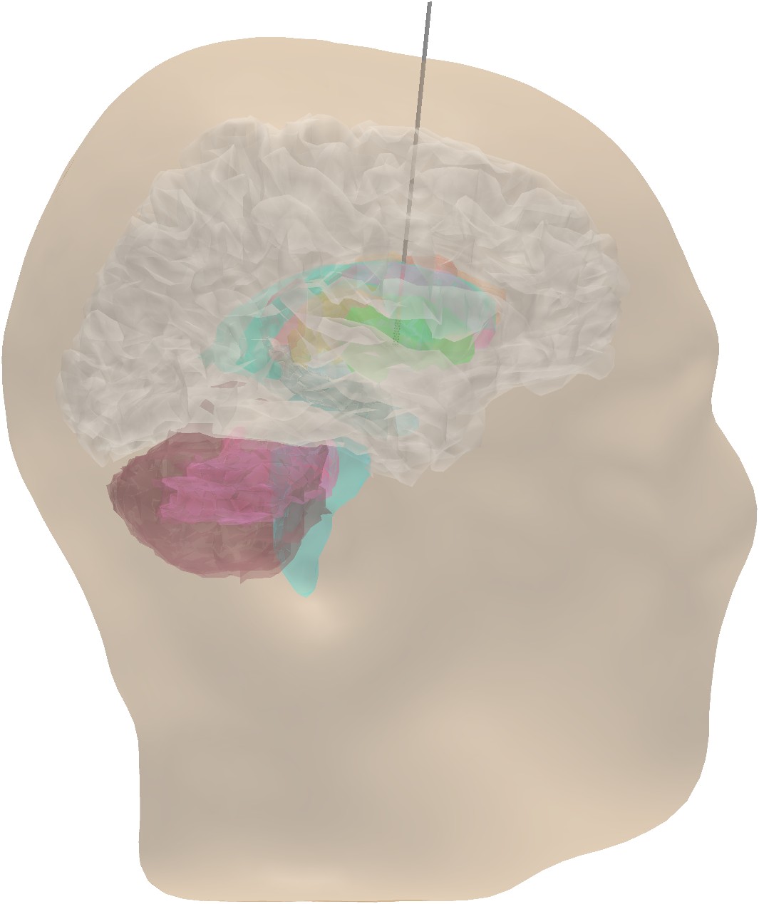
(a) Segmented head model domain depicting main subcortical structures.

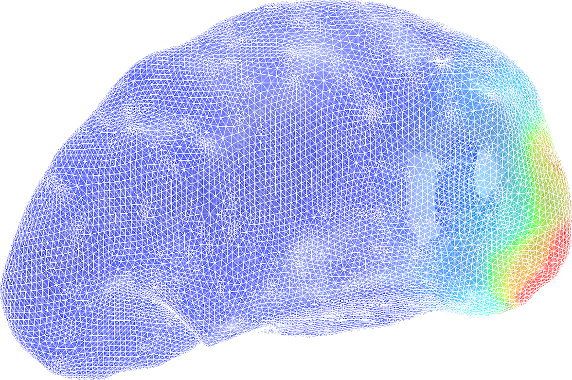
(b) Refined and boundary-fitted thalamus sub-compartment.

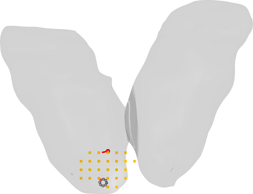
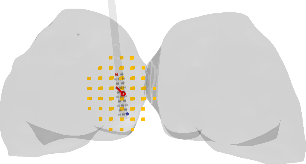
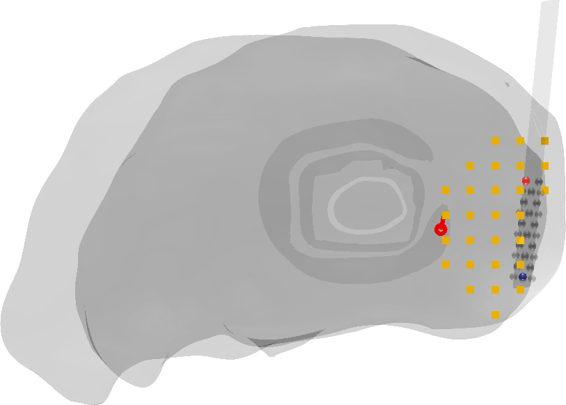
(c) Superior, coronal, and sagittal view of target domain. The interthalamic adhesion can be easily noticed.

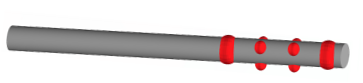
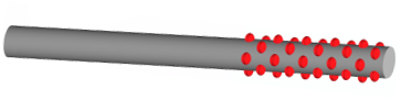
(d) 8- and 40-electrode contacts, respectively.

Figure 1: (1(a)): A head model including skull, forebrain, midbrain, hindbrain structures as well as directional deep brain stimulation (dDBS) lead positioned at the right-hemispheric anterior nucleus of thalamus (ANT). (1(b)): Refined and boundary-fitted thalamus sub-compartment with the distribution of tetrahedral mesh edges and an interpolated current intensity distribution shown on the surface. (1(c)): Placement of a 40-contact dDBS lead with a bipolar electrode configuration (anodal as red, and cathodal as blue). The dipolar target current (red) is depicted by the red pin, indicating the target position and orientation; a 6.0 millimeter (mm) region of interest (ROI) is displayed as an arrangement of source points (yellow squares) for High-Resolution Lead Field (HR-LF) matrix. (1(d)): Probing strategy of the 8- and 40-electrode contacts inspired by Abbott’s St. Jude Medical Infinity™ Directional Lead 6180 model and Medtronic-Sapiens, respectively.

2.2 Lead Field Matrix

The linear forward mapping can be formulated as a real $N\times K$ lead field matrix $\hat{\bf L}$, which relates current injections at the electrodes to the resulting volumetric current density distribution across different electrode configurations. This matrix characterizes the numerical relationship between the real $K\times 1$ current pattern ${\bf y=(y_{1},\ldots,y_{K})}$ and the real $N\times 1$ discretized volume current density $\hat{\bf x}=(\hat{x}_{1},\hat{x}_{2},\ldots,\hat{x}_{N})$. The latter variable represents an arrangement of uniformly distributed source points within the target domain, each with three degrees of freedom (DOFs) corresponding to three dipolar unit currents with Cartesian orientations.

We generate a lead field matrix for two different resolution levels: (i) Low-Resolution Lead Field (LR-LF), which corresponds to a target set of 244 $\times$ 3 spatial DOFs that cover the entire thalamus compartment. This robust interpretation offers a functional assessment of the model, serving as a benchmark for our numerical experiments. To validate whether our minimal interpretation is adequate, we compare the volumetric current density distribution with a locally detailed lead field matrix, (ii) High-Resolution Lead Field (HR-LF). This matrix consists of 3620 $\times$ 3 DOFs distributed across the thalamus, meaning that the mutual distance between nearest neighboring DOFs is reduced by 40% compared to LR-LF. Due to the increased computational cost of using a larger lead field size, our examination of HR-LF is confined to a spherical region of interest with a 6.0 mm radius, co-centered with the lead model (Fig. 1(c)).

2.3 Probing Strategy

The length of the current pattern vector $\mathbf{y}$ corresponds to the number of contacts on the DBS lead. We consider two models: an 8-contact model with diameter and contact placement matching Abbott’s St. Jude Medical Infinity^TM Directional Lead 6180, and a more complex 40-contact model dimensionally aligned with the Medtronic-Sapiens design (Fig. 1(d)). The 8-contact lead consists of four cylindrical groups of contact bands, with centers separated by 2.0 mm (1.5 mm contact length and 0.5 mm separation), and two middle circular electrodes partitioned axially into three sections (a ”1-3-3-1” configuration). The 40-contact model consists of 40 contacts arranged in 8 rows, each containing 5 ellipsoidal contacts (width 0.8 mm, height 0.66 mm), with a 1.5 mm separation and a 0.75 mm longitudinal shift between neighboring rows. Both leads share the same diameter of 1.27 mm. For simplicity, each contact is modeled as a spherical surface with a contact impedance of 2.0 k$\Omega$ (kiloohms) [49].

The maximum total current injection supplied by all the active electrodes is limited to 4.0 mA (milliamperes) (5), and the maximum current per electrode contact is set to $\pm$ 2.0 mA (6). This can be considered a moderately typical setting, for example, 3.0 mA as a reference for monopolar patterns in [50]. The total absolute sum of electric potential corresponding to the contacts in the lead is normalized to meet the intended maximum current injection value (7). As a reference threshold for neural activation, we consider the current amplitude of 3.85 A/m² (amperes per square meter) [51], which falls within the excitation current thresholds of 2.5 to 6.0 A/m² estimated for nerve fibers in the upper limb area of the motor cortex at frequencies of 50.0 Hz and 2.44 kHz [52]. Our optimization framework maintains this reference threshold constant across all tested configurations. By holding temporal characteristics constant, we ensure that the observed variations in activation patterns arise from differences in spatial registrations and current steering, rather than from stimulation timing. This choice follows the framework established in previous studies by Deli et al. [53] and Schlaepfer et al. [54], where monopolar and bipolar stimulation configurations were evaluated using a consistent stimulation protocol, specifically maintaining a pulse width of 60 µs and a frequency of 130 Hz across all conditions. This design allowed the authors to isolate the effects attributable solely to electrode configuration by holding other key stimulation parameters constant, with amplitude as the only adjusted variable.

2.4 Optimization Algorithms

The aim of this study is the application of mathematical optimization algorithms to retrieve the current pattern ${\bf y}$ (4) within the local target region, aiming to optimally match the volumetric current distribution generated by the target current dipole modeling [55, 56, 51]. To quantify the optimal electrode configurations derived from the algorithm, we compare them based on the decision variables $\Gamma$, $\Xi$, and $\Theta$, as delineated by the optimization paradigm. The focused current density $\Gamma$ (A/m²) is defined as

$${\Gamma}=\frac{{\bf x}_{1}^{T}{\bf L}_{1}{\bf y}}{\|{\bf x}_{1}\|_{2}}.$$

The focality of the stimulation, or field ratio, $\Theta$, is defined as the ratio of the focused current density divided by the undesired nuisance current density ($\Xi$) and is defined as

$${\Theta}=\frac{{\Gamma}}{\Xi}\quad\hbox{with}\quad\Xi=\frac{\|{\bf L}_{2}{\bf y}\|_{2}}{\sqrt{M}}.$$

2.4.1 Bipolar Configurations

Bipolar configurations are derived through the reciprocity principle (RP) [36]. The principle states that the maximum focused current density, i.e., $\Gamma_{\hbox{\scriptsize{max}}}$, of an applied linear system can be achieved by limiting the electrode configuration to a pair of anodal and cathodal electrode contacts (Fig. 3). This configuration is obtained by multiplying the dipolar target current distribution by the transpose of the lead field matrix, selecting both the greatest positive and negative poles, and setting the remaining electrodes in the lead to zero. The reciprocity principle aims at maximizing current density at the expense of field ratio fidelity.

2.4.2 Multipolar Configurations

Multipolar configurations, i.e., leads with multiple active electrode contacts, are obtained via convex optimization techniques such as L1-norm regularized L1-norm fitting (L1L1) [32] and through Tikhonov-Regularized Least Squares (TLS) [37, 38] methods. Both methods employ a metaheuristic search strategy to explore only a carefully chosen fraction of an otherwise huge search space—trading guaranteed optimality for scalability and adaptability—to handle large, ill-behaved, or poorly understood problems within practical time and memory constraints [57]. The candidate solution is the one that can achieve the highest ratio between the (target) current density at the stimulation site and that in the surrounding adjacent areas (referred here to as nuisance current). The determination of this solution is defined by tuning a set of predefined hyperparameters along with the current pattern ${\bf y}$, subject to specific metacriteria, namely, maximizing the field ratio while ensuring $\Gamma\geq\Gamma_{0}>0$, thereby maintaining sufficient intensity at the target location (with $\Gamma_{0}=0.80$ mA in this case). Without a lower bound for intensity $\Gamma$, the intensity of the $\Theta$-maximizer is likely to diminish. A rough upper bound is provided as a L1-norm fitting threshold to suppress nuisance current density $\Xi$. In contrast, traditional least-squares formulations tend to produce smoothly distributed currents, which may be clinically suboptimal, as focal and sparse activation is often preferred to minimize side effects and enhance therapeutic precision. Moreover, least-squares approaches are sensitive to noise and outliers, often yielding non-robust solutions [58]. Detailed formulation of both the L1L1 and TLS methods is provided in A.

2.5 Uncertainty Modeling

Uncertainty refers to various physiological and technical factors that directly or indirectly affect the accuracy and reliability of the stimulation, including imprecision in lead placement, patient-specific anatomical variation, and inhomogeneities in tissue conductivity. In this study, all sources of uncertainty affecting the optimization problem are modeled as additive perturbations to the lead field. While this Gaussian noise model is a simplification, it enables a tractable first-step analysis of robustness. We acknowledge that in practice, the true uncertainty arises from a variety of unrelated sources.

(a) Left: The set $\mathcal{V}_{\delta}$ corresponding to PSNR $\delta^{-1}$ following from the uncertainty factors is shown by the blue dashed circle with radius $d_{\delta}$. The target is at the distance $d_{T}$ from the probe. Between the target and the boundary of $\mathcal{V}_{\delta}$ is a range $d_{\varepsilon}$ in which the lead field decays by the factor $\varepsilon$, which approximates the maximum achievable dynamic range $\varepsilon$ between the focused current density at the target position and in its surroundings. Right: One-dimensional interpretation of the lead field decay.

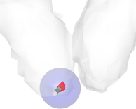
$\mathcal{V}_{-10\text{ dB}}$

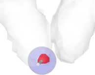
$\mathcal{V}_{-20\text{ dB}}$

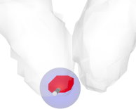
$\mathcal{V}_{-30\text{ dB}}$

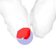
$\mathcal{V}_{-40\text{ dB}}$

(b) The set $\mathcal{V}_{\delta}$ illustrated for the volumetric model of this study with respect to PSNR $\delta^{-1}$ levels from 10 to 40 dB.

Figure 2: (2(a)): A schematic of how the peak signal-to-noise ratio (PSNR) $\delta^{-1}$ relates to the set $\mathcal{V}_{\delta}$ and to the approximate maximum dynamic range $\varepsilon^{-1}$ of the volumetric stimulation current field. (2(b)): The set $\mathcal{V}_{\delta}$ shown for PSNR 10–40 dB, providing a rough approximation of the maximum feasible coverage of volume of tissue activated (VTA) for an activation threshold set by $\delta$.

8-contact Electrode Configuration

RP

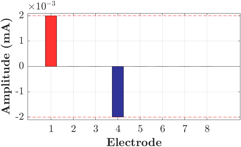
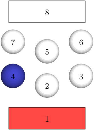
L1L1(A)

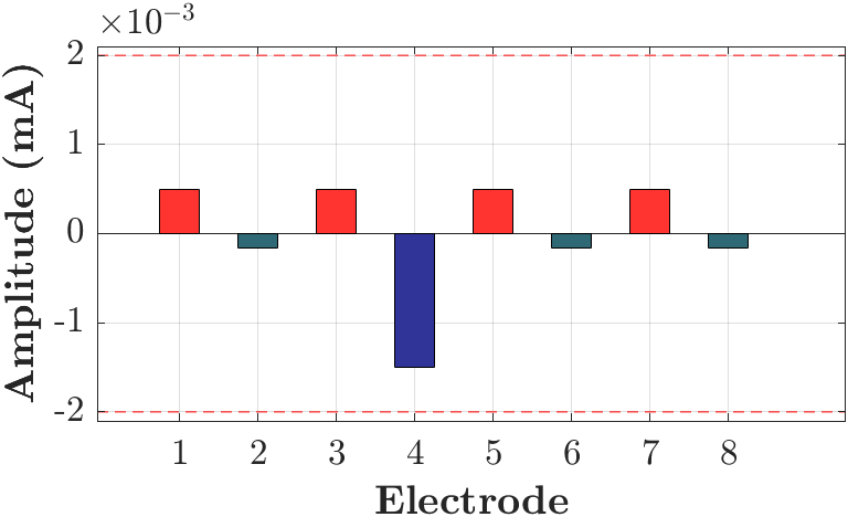
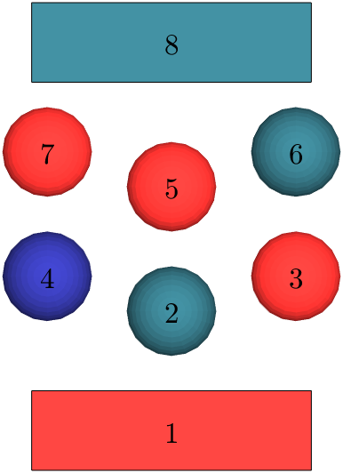
L1L1(B)

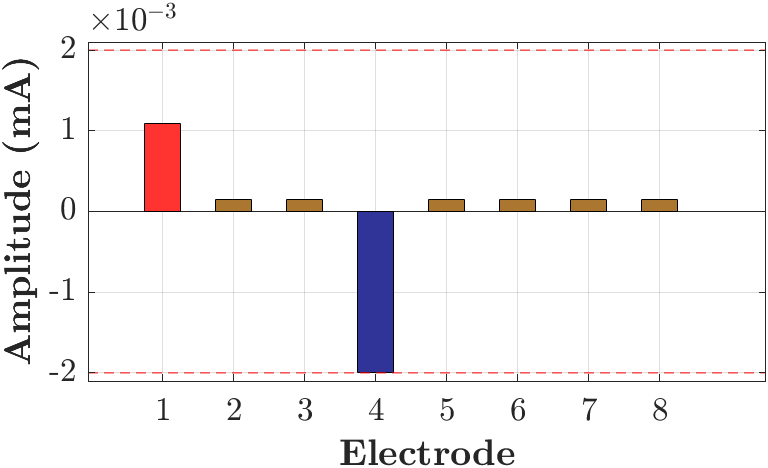
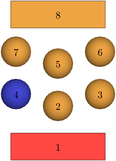
TLS

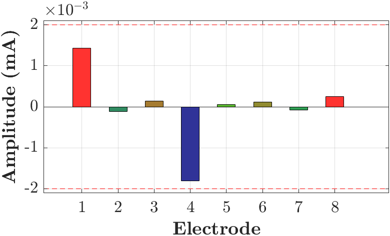
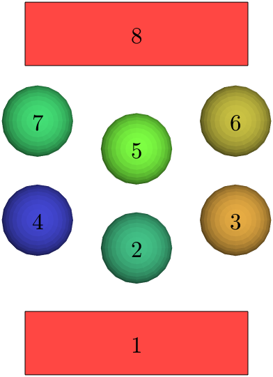
40-contact Electrode Configuration

RP

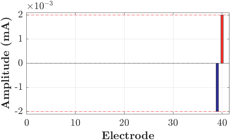
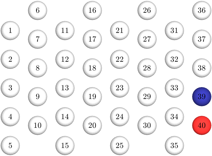
L1L1(A)

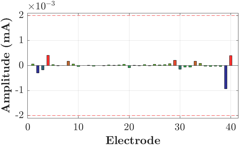
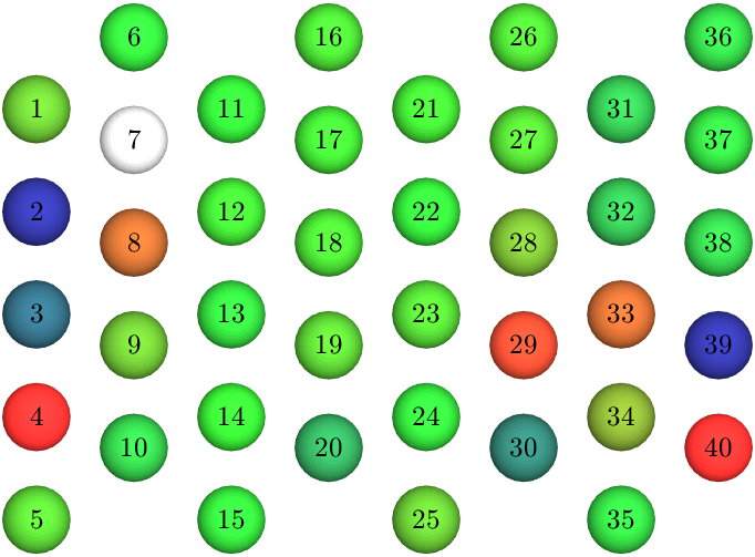
L1L1(B)

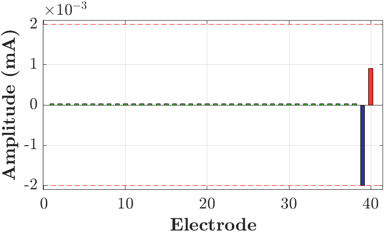
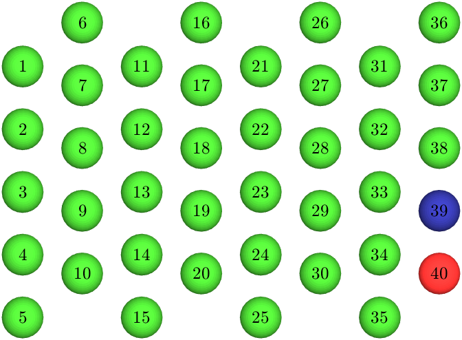
TLS

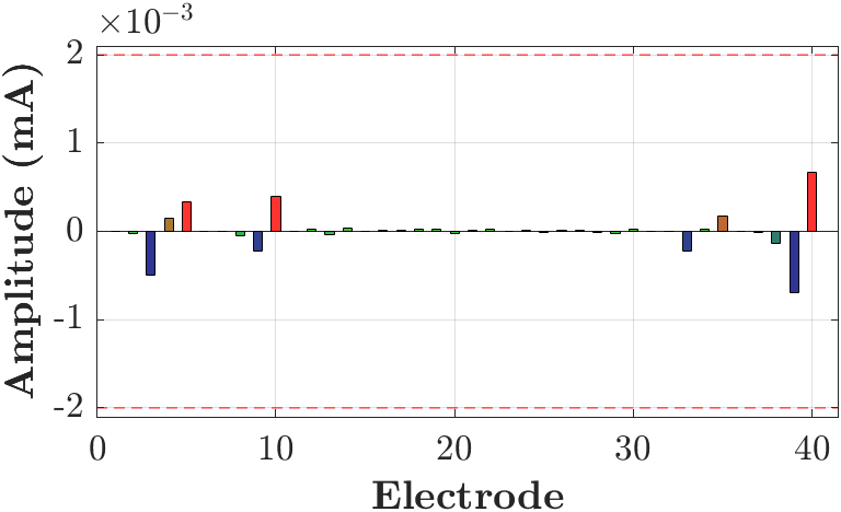
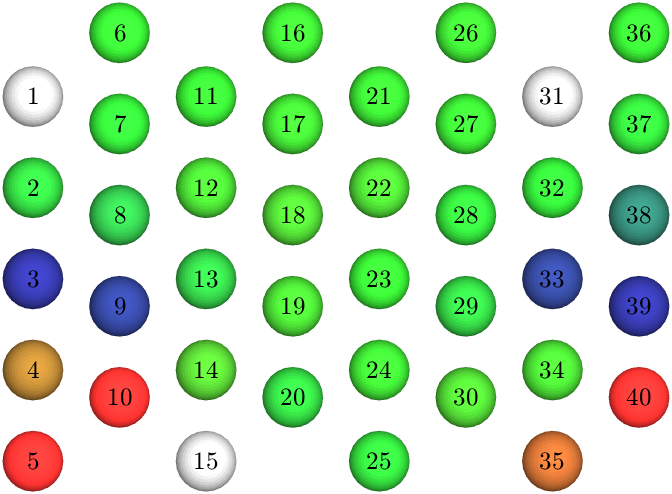
Figure 3: Examples of current injection patterns obtained using the Reciprocity Principle (RP), metaheuristic L1-norm regularized L1-norm fitting (L1L1) method under two different nuisance current thresholds (L1L1(A) with $\varepsilon=\{0:-160\}$ and L1L1(B) with $\varepsilon=\{0:-10\}$), and the Tikhonov-Regularized Least Square (TLS) method. The target position and orientation (parallel to the lead) is indicated by the red upward pin. The bar plots display the resulting electrode current amplitudes, while the contact maps visualize their spatial distribution over the electrodes; cathodal (blue), anodal (red), and inactive (gray/green). The RP method yields a bipolar configuration maximizing focused current density $\Gamma$, while the remaining methods searches for a multipolar configuration maximizing focality $\Theta=\Gamma/\Xi$ under an a priori constraint $\varepsilon$ on the nuisance current density $\Xi$, determined by the peak signal-to-noise ratio (PSNR) $\delta^{-1}$ and the lead field attenuation. The L1L1(B) result reflects more strongly constrained $\Xi$ (smaller dynamic range), activating fewer contacts whereas L1L1(A) and TLS allow higher $\Theta$ values and broader excitation patterns. The voltage/current on the electrode contacts are $\pm 2.0$ mA (milliamperes).

We postulate that the volumetric current density distribution can be optimized for those degrees of freedom indexed by $i$, where the L2-norm (2-norm) $\|{\bf\tilde{l}}_{i}\|_{2}$ of the corresponding reduced lead field matrix row remains above the threshold. This row, denoted as ${\bf l}_{i}$, is first reduced (as described in Appendix 9) and then zero-averaged, taking the form

$$\tilde{\bf l}_{i}=\left(L_{i,1}-\overline{L}_{i},L_{i,2}-\overline{L}_{i},\dots,L_{i,K}-\overline{L}_{i}\right),$$

where $\overline{L}_{i}=K^{-1}\sum_{j=1}^{K}L_{i,j}$ represents the mean of the row entries. The threshold for optimization is determined by a peak signal-to-noise ratio (PSNR) constraint, ensuring that only degrees of freedom with a sufficiently strong contribution to the lead field are considered in the optimization process. We define the feasible set of degrees of freedom as

$$\mathcal{V}_{\delta}=\{i\,|\,\|{\bf\tilde{l}}_{i}\|_{2}\geq\delta\max_{k}\|{\bf\tilde{l}}_{k}\|_{2}\},$$

where $\max_{k}\|{\bf\tilde{l}}_{k}\|_{2}$ is the maximum L2-norm of the zero-averaged lead field rows. The parameter $\delta$ sets a relative threshold, filtering out degrees of freedom whose contributions are too weak to be considered meaningful. If $\delta$ is chosen to represent neural activation threshold, then $\mathcal{V}_{\delta}$ serves as an approximation of the maximum VTA (Fig. 2(a)).

Since lead field attenuation and uncertainty impose fundamental limits on stimulation accuracy, the PSNR constraint defines the theoretical limit of the optimization performance. If the target stimulation site corresponds to the $\ell$-th index, then the maximum achievable dynamic range $\varepsilon^{-1}$ between the current density at the target site and its surroundings is approximately

$$\varepsilon\geq\delta\,\|{\bf\tilde{l}}_{\ell}\|_{2}^{-1}\max_{k}\|{\bf\tilde{l}}_{k}\|_{2}.$$

This relationship indicates that the minimum contrast in current density between the target location and surrounding regions is constrained by $\delta$ and the structure of the lead field matrix (Fig. 2(b)).

2.6 Numerical Experiments

Our numerical experiments are designed to evaluate the performance of the proposed optimization methods with respect to: (i) simulated 8-contact and 40-contact DBS lead configurations, (ii) noiseless and noisy forward mappings, (iii) orientation of the current dipole in the model (parallel or perpendicular with respect to the lead array) [17], and (iv) algorithm efficiency. The hardware used for these experiments includes a Dell Precision 5820 Workstation with 256 GB of RAM, a 10-core Intel i9–10900X CPU, and an NVidia Quadro RTX 4000 GPU. The GPU (graphics processing unit) was utilized to accelerate both forward and inverse computations.

Table 1: Summary of the proposed optimization methods. While the RP provides a bipolar reciprocal of the target, both L1L1 and TLS constitute a metaheuristic search over a two-dimensional hyperparameter lattice. L1L1 is subdivided into L1L1(A) and L1L1(B) based on two alternative a priori assumptions of the feasible $\varepsilon$ threshold range which is [-160, 0] and [-10, 0] dB, respectively. The regularization and the L2-norm weighting parameter intervals are chosen as in [32]. CPU time refers to the computing time needed to evaluate a single optimizer with fixed hyperparameter values for HR-LF with the 40-contact lead configuration.

		Hyperparameter		CPU
		Tuning Range	Role	Time
Method	Search Type	(dB)		(s)
RP	Reciprocal	–	–	5.7E-03
L1L1(A)	Metaheuristic	$\alpha\in[-100,-30]$	Regularization	6.0
		$\varepsilon\in[-160,0]$	Threshold
L1L1(B)	Metaheuristic	$\alpha\in[-100,-30]$	Regularization	3.7
		$\varepsilon\in[-10,0]$	Threshold
TLS	Metaheuristic	$\gamma\in[-200,-110]$	Regularization	5.0E-02
		$\beta\in[-50,40]$	Weight

The L1L1 method is examined using two alternative a priori assumptions for the feasible $\varepsilon$ threshold range: [-160, 0] dB and [-10, 0] dB, respectively. We refer to these settings as ”L1L1(A)” and ”L1L1(B)”. The former setting neglects the effect of uncertainty on the field ratio $\Theta$, while the second assumes that uncertainty is included within 10 dB dynamic range. As for TLS method, the regularization parameter $\gamma$ and the L2-norm weighting parameter $\beta$ intervals are chosen as in [32] (Table 1).

Gaussian noise is added to the lead field to examine spatial sensitivity; the effect of noise is assessed in an overall setting, where the candidate solution is determined for each target DOF of LR-LF under PSNR 40.0 dB noise corruption. While anatomical variations may cause spatially correlated errors, the implementation of noise offers a generic and tractable way to assess noise-robustness when the exact structure of uncertainty is unknown. It serves as a standard baseline for evaluating sensitivity to model perturbations.

The noise sensitivity is examined for two specific target positions (I) and (II) (Fig. 4) using PSNRs of 40.0 and 50.0 dB, along the HR-LF. When interpreted in terms of $\mathcal{V}_{\delta}$ (Figure 2(b)), PSNR 40.0 dB (50.0 dB) corresponds to the assumption that each possible target position in the set $\mathcal{V}_{-30\text{ dB}}$ ($\mathcal{V}_{-40\text{ dB}}$) can be stimulated with at least a 10 dB dynamic range $\varepsilon^{-1}$ for $\Theta$. This assumption aligns well with the $\varepsilon$ range of $[-10,0]$ selected for L1L1(B).

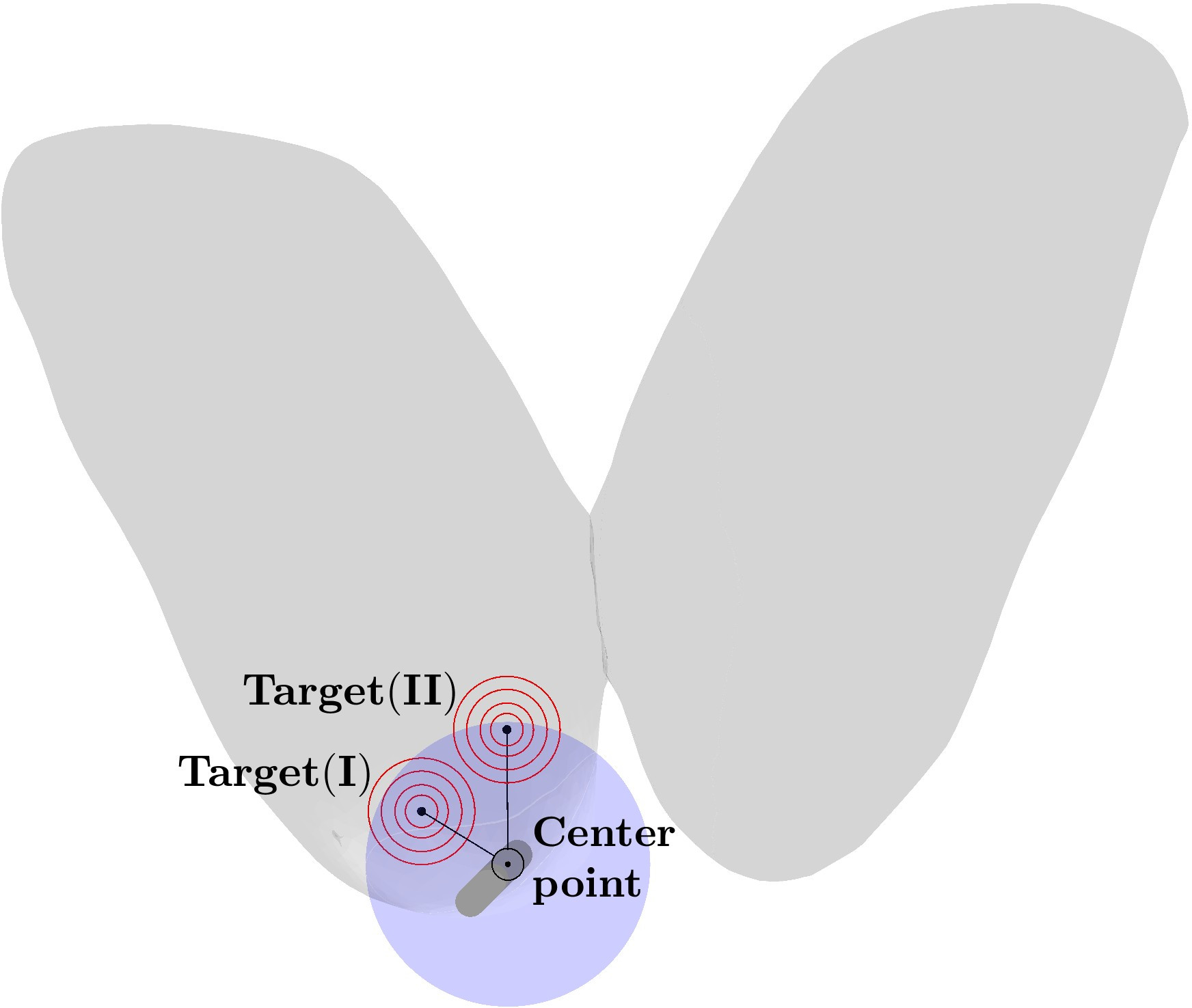
Figure 4: Visualization of the two synthetic stimulation targets, Target (I) and Target (II), analyzed separately in numerical experiments. Both targets are positioned within the right thalamus near a directional DBS lead. The figure also displays the lead’s center point and a concentric spherical region of interest (ROI) with 6 mm radius, representing an approximate VTA. This ROI defines the region where maximizing stimulation intensity while minimizing current spread to surrounding areas is considered feasible. As targets (I) and (II) are not right next to the probe, lead field uncertainty affects the optimization process. Bilateral thalamic structures are shown in gray for anatomical reference.

	LR-LF			HR-LF
	Focused $\Gamma$ (A/m2)	Nuisance $\Xi$ (A/m2)	Ratio $\Theta$ (rel.)	Focused $\Gamma$ (A/m2)	Nuisance $\Xi$ (A/m2)	Ratio $\Theta$ (rel.)
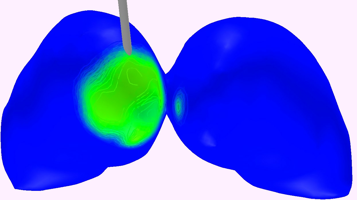
[HTML]fff0ff	[HTML]fff0ff	[HTML]fff0ff	[HTML]fff0ff	[HTML]fff0ff	[HTML]fff0ff	[HTML]fff0ff
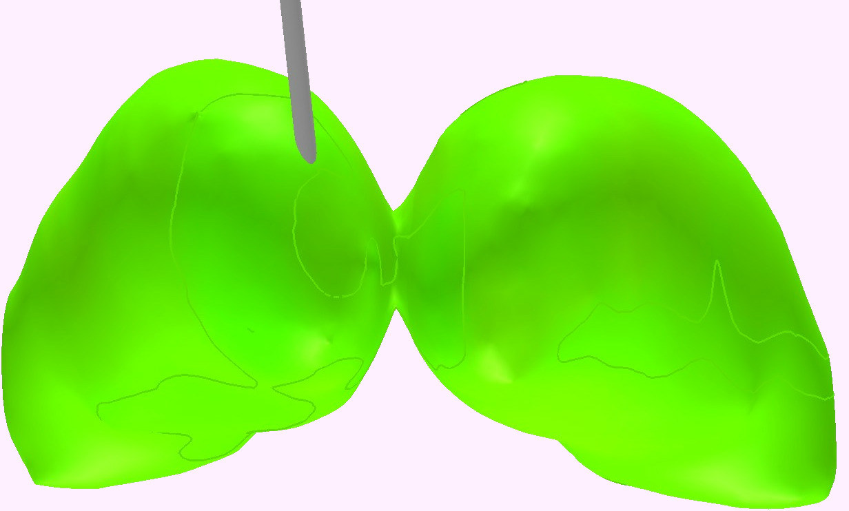
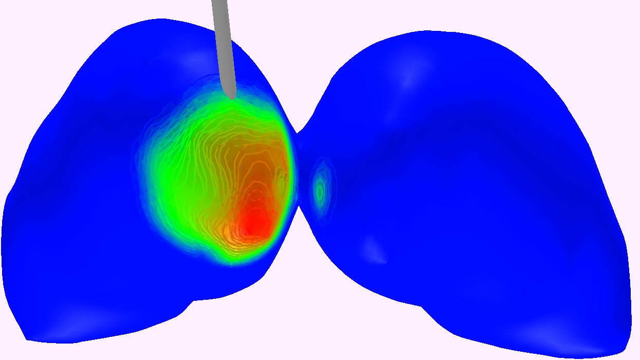
[HTML]fff0ff RP   Perpendicular   Parallel	[HTML]fff0ff	[HTML]fff0ff	[HTML]fff0ff	[HTML]fff0ff	[HTML]fff0ff	[HTML]fff0ff
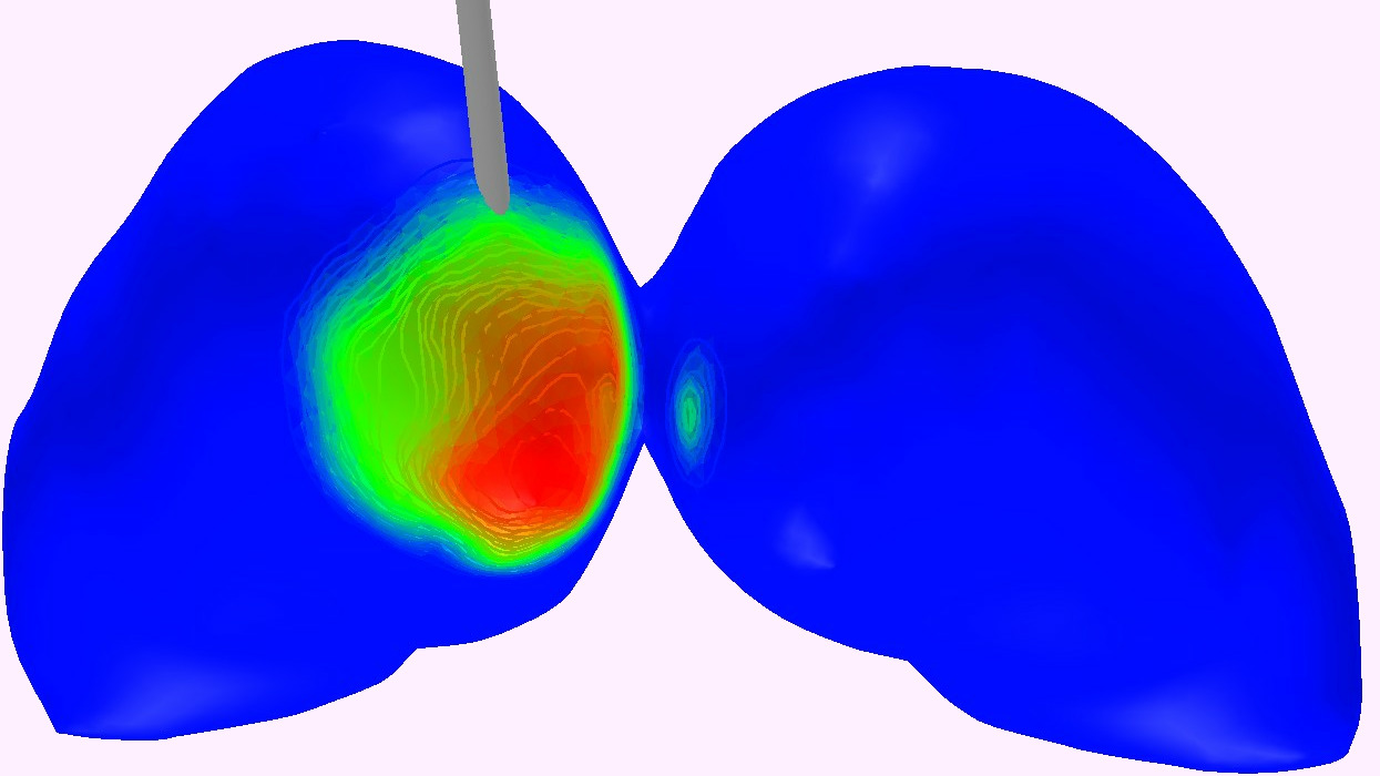
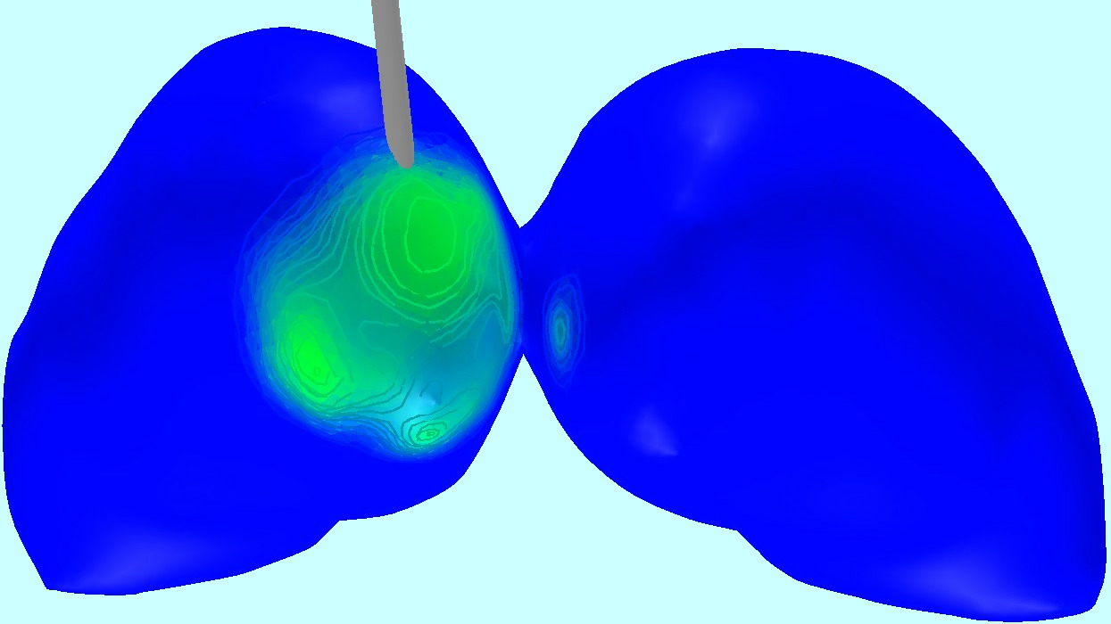
[HTML]ccffff	[HTML]ccffff	[HTML]ccffff	[HTML]ccffff	[HTML]ccffff	[HTML]ccffff	[HTML]ccffff
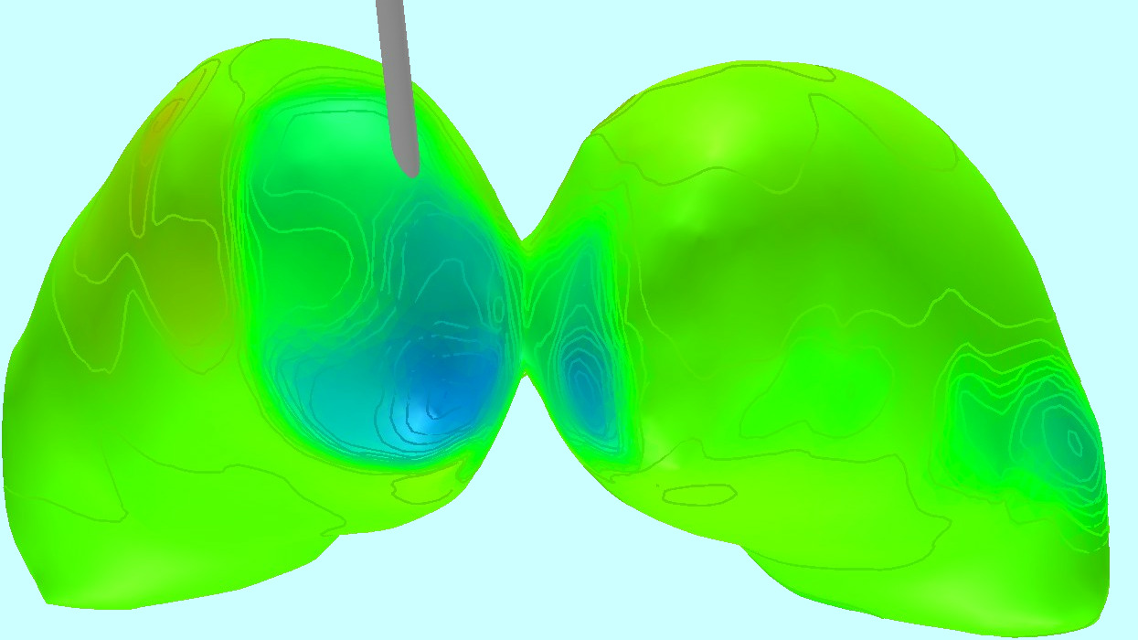
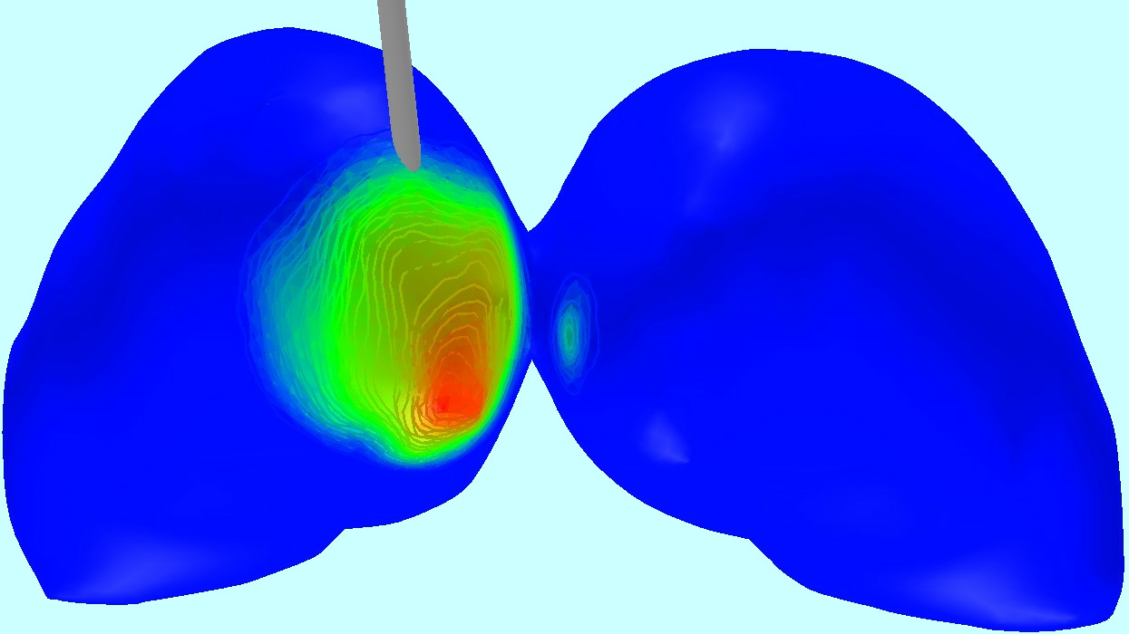
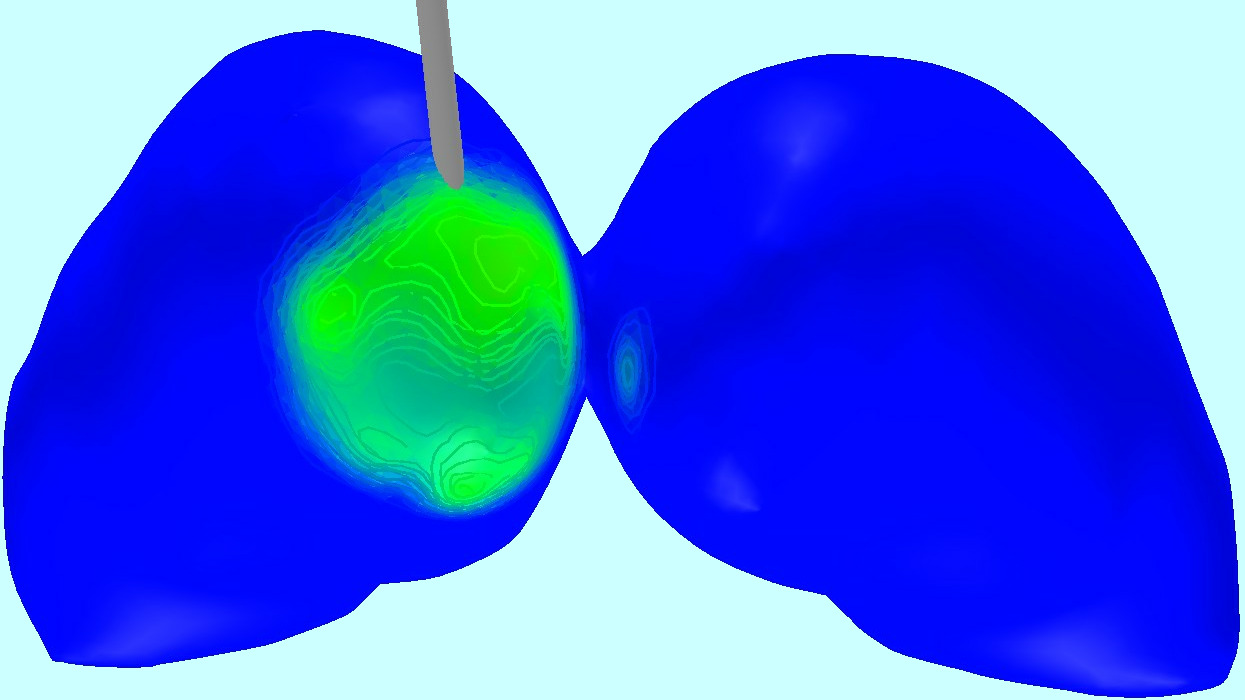
[HTML]ccffff L1L1(B), $\varepsilon\in[-10,0]$ dB   Perpendicular   Parallel	[HTML]ccffff	[HTML]ccffff	[HTML]ccffff	[HTML]ccffff	[HTML]ccffff	[HTML]ccffff
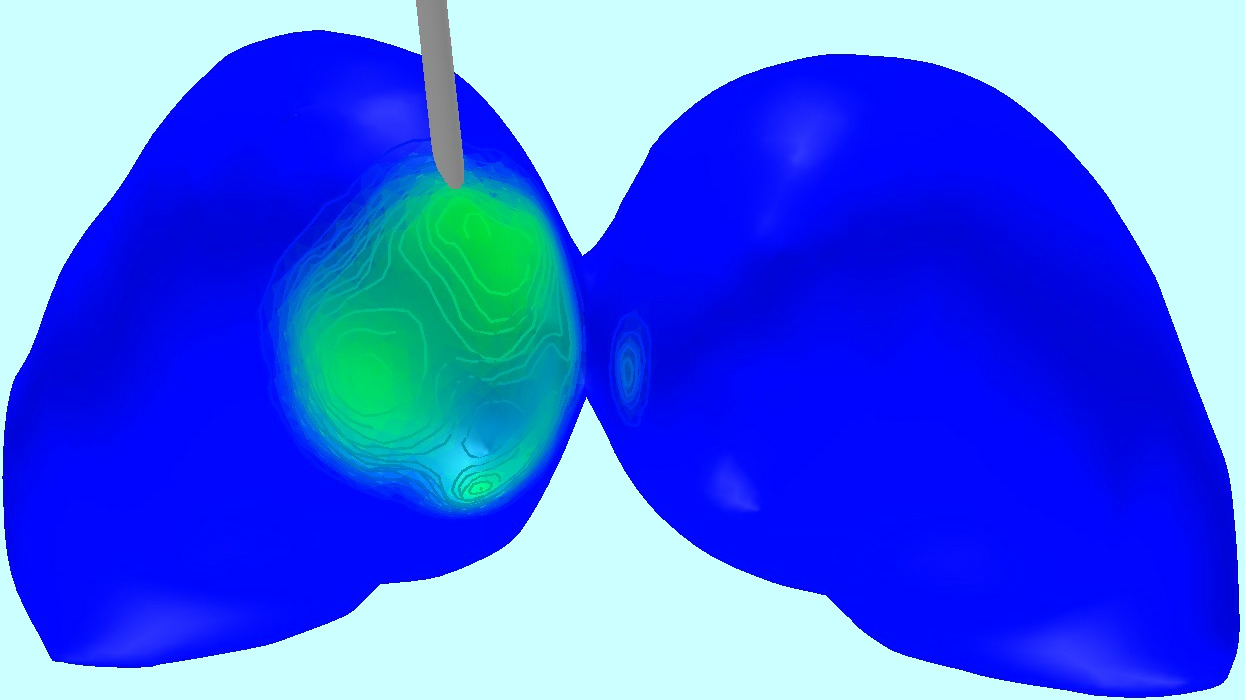
[HTML]ccffff	[HTML]ccffff	[HTML]ccffff	[HTML]ccffff	[HTML]ccffff	[HTML]ccffff	[HTML]ccffff
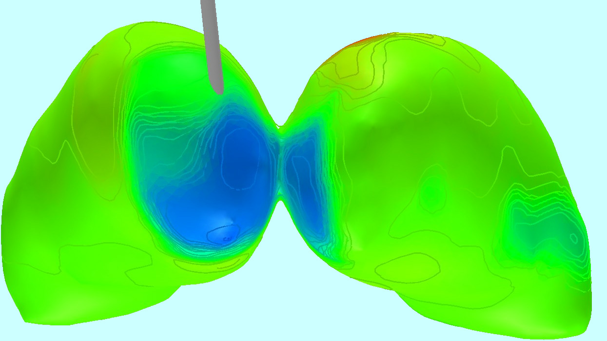
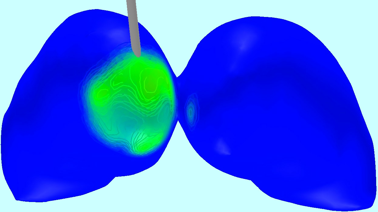
[HTML]ccffff L1L1(A), $\varepsilon\in[-160,0]$ dB   Perpendicular   Parallel	[HTML]ccffff	[HTML]ccffff	[HTML]ccffff	[HTML]ccffff	[HTML]ccffff	[HTML]ccffff
[HTML]e5ffd4	[HTML]e5ffd4	[HTML]e5ffd4	[HTML]e5ffd4	[HTML]e5ffd4	[HTML]e5ffd4	[HTML]e5ffd4
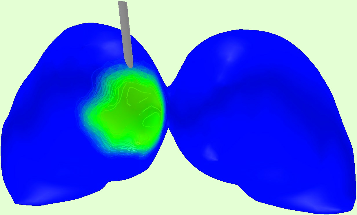
[HTML]e5ffd4 TLS, $\beta\in[-50,40]$ dB   Perpendicular   Parallel	[HTML]e5ffd4	[HTML]e5ffd4	[HTML]e5ffd4	[HTML]e5ffd4	[HTML]e5ffd4	[HTML]e5ffd4

Figure 5: Volumetric optimization results for the 8-contact probe and noiseless lead fields. Decision variable $\Gamma$, $\Xi$ and $\Theta$ for optimizers found via RP, TLS, L1L1(A), and L1L1(B) method illustrated as a function of the target position and orientation (parallel or perpendicular w.r.t. the probe). Left: distributions for a (i) Low-Resolution Lead Field (LR-LF) where the spatial degrees of freedom (DOFs) cover both thalamus lobes. Right: distribution for a (ii) High-Resolution Lead Field (HR-LF) where the DOFs is confined to a region of interest within a radius of 6.0 mm (millimeters) from the center of the lead. The optimal electrode configuration found by the L1L1 method maximizes the field ratio $\Theta$ subject to $\Gamma>=\Gamma_{0}$. The $\Theta$ distribution found using L1L1(A) is elevated as compared to the case of RP and TLS. The limited dynamic range ($\varepsilon$ range) of L1L1(B) is reflected in an overall slightly lower $\Theta$.

	LR-LF			HR-LF
	Focused $\Gamma$ (A/m2)	Nuisance $\Xi$ (A/m2)	Ratio $\Theta$ (rel.)	Focused $\Gamma$ (A/m2)	Nuisance $\Xi$ (A/m2)	Ratio $\Theta$ (rel.)
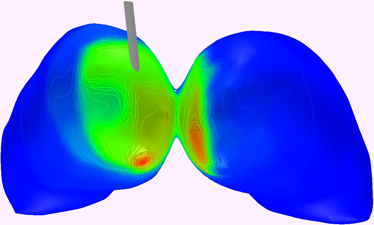
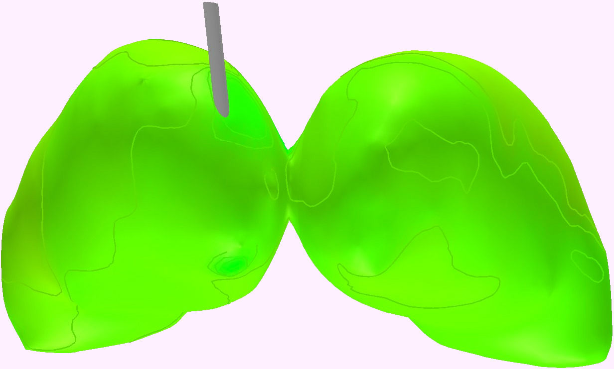
[HTML]fff0ff	[HTML]fff0ff	[HTML]fff0ff	[HTML]fff0ff	[HTML]fff0ff	[HTML]fff0ff	[HTML]fff0ff
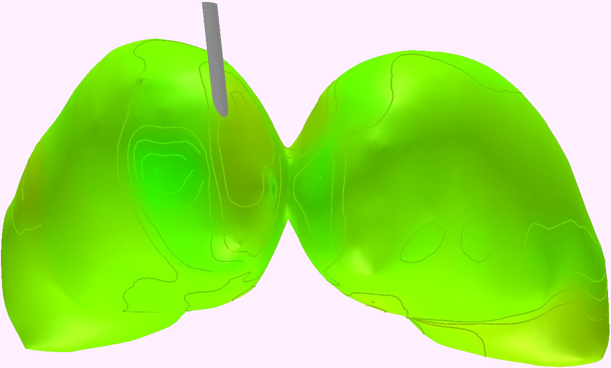
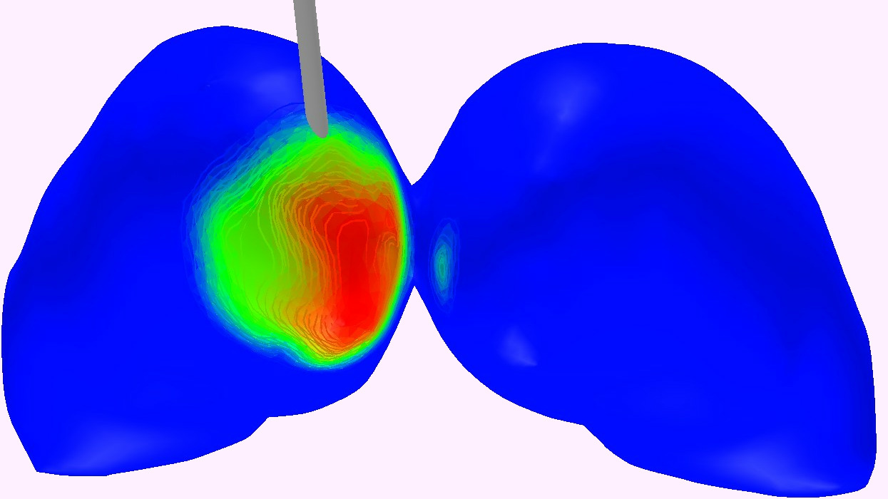
[HTML]fff0ff RP   Perpendicular   Parallel	[HTML]fff0ff	[HTML]fff0ff	[HTML]fff0ff	[HTML]fff0ff	[HTML]fff0ff	[HTML]fff0ff
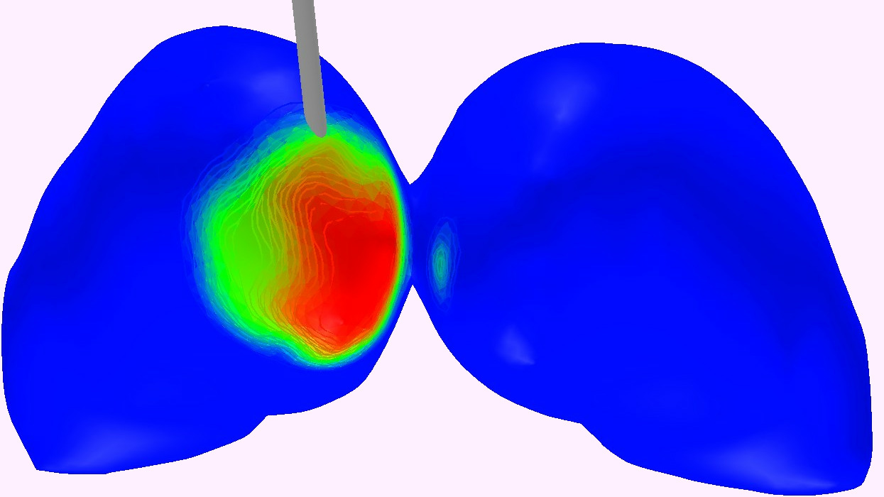
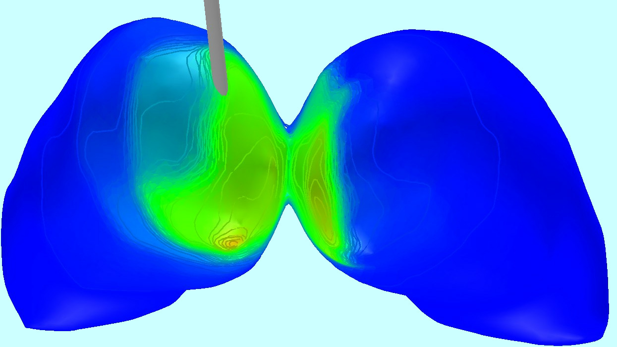
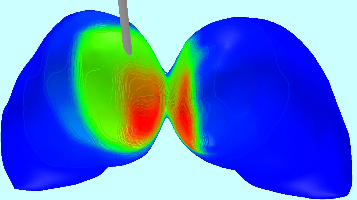
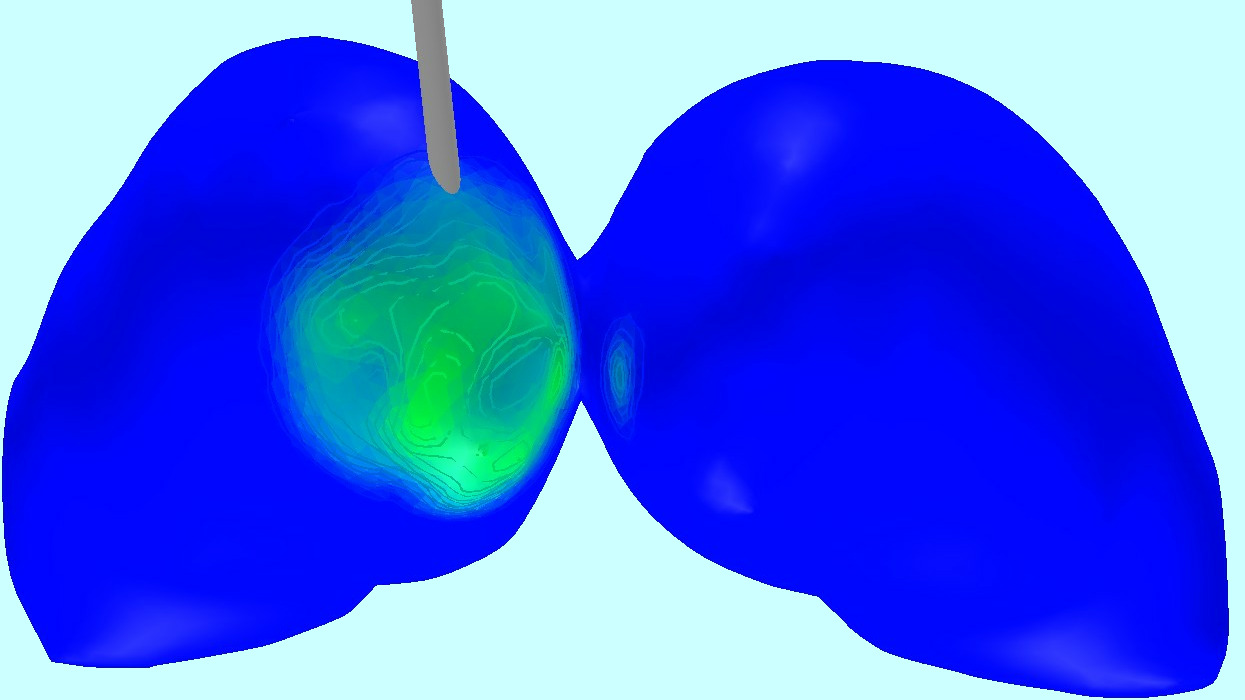
[HTML]ccffff	[HTML]ccffff	[HTML]ccffff	[HTML]ccffff	[HTML]ccffff	[HTML]ccffff	[HTML]ccffff
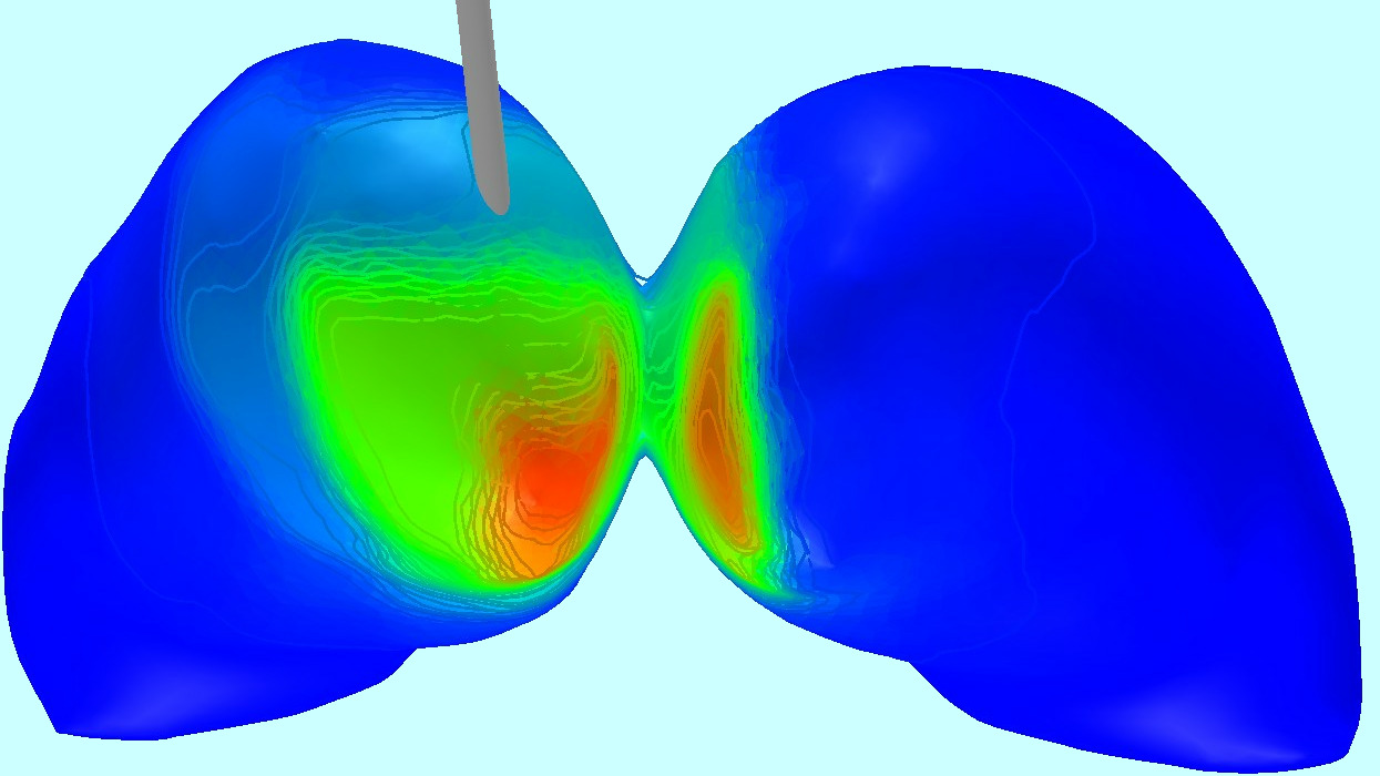
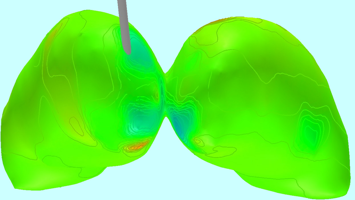
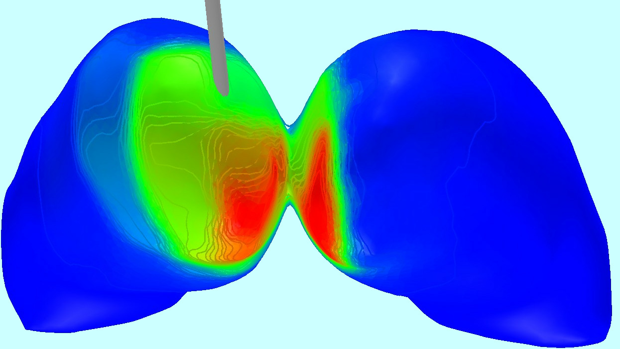
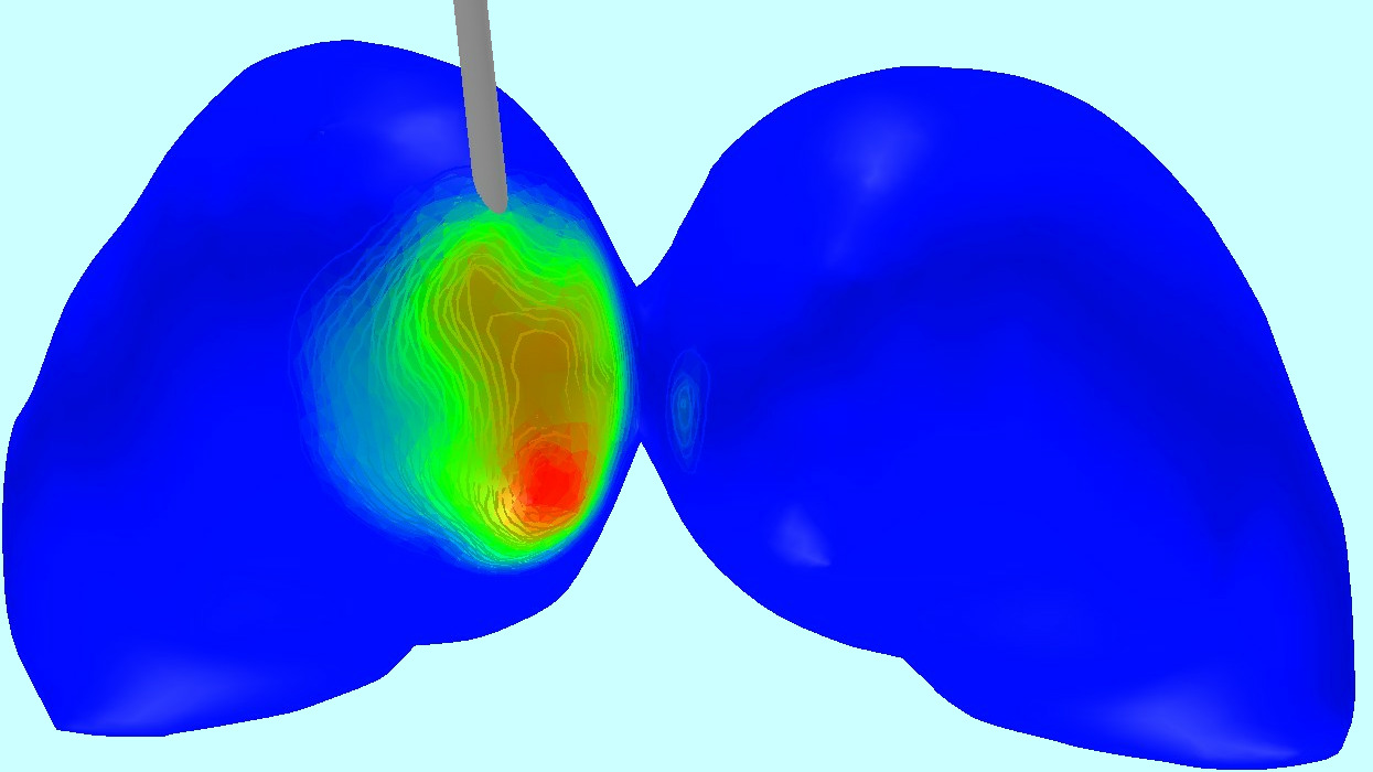
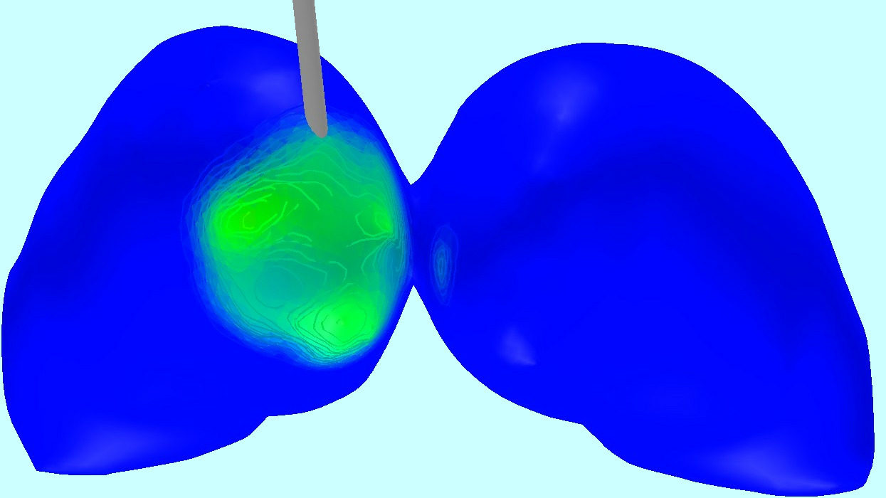
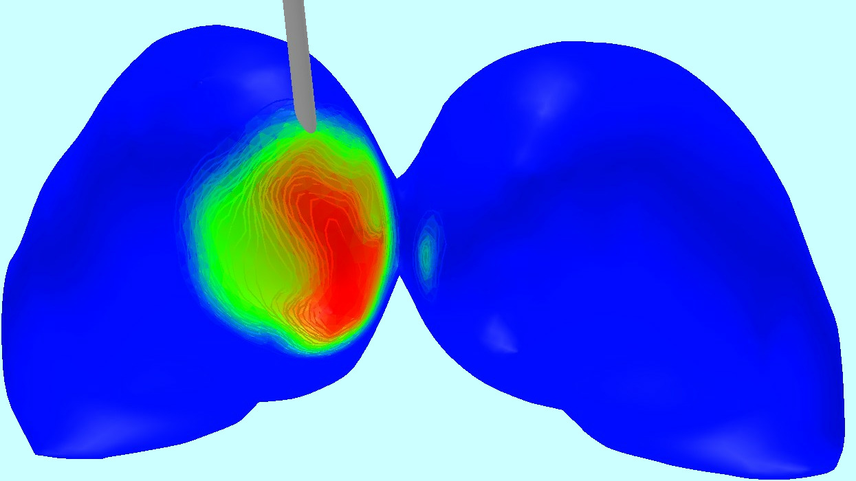
[HTML]ccffff L1L1(B), $\varepsilon\in[-10,0]$ dB   Perpendicular   Parallel	[HTML]ccffff	[HTML]ccffff	[HTML]ccffff	[HTML]ccffff	[HTML]ccffff	[HTML]ccffff
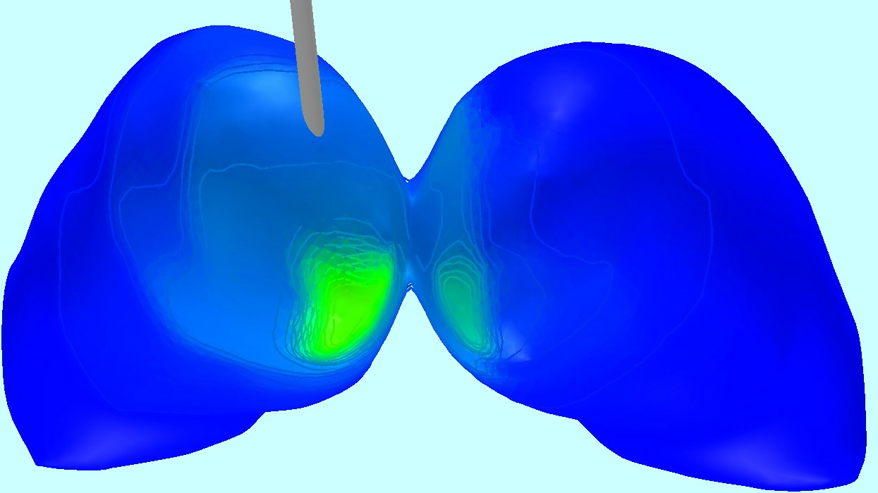
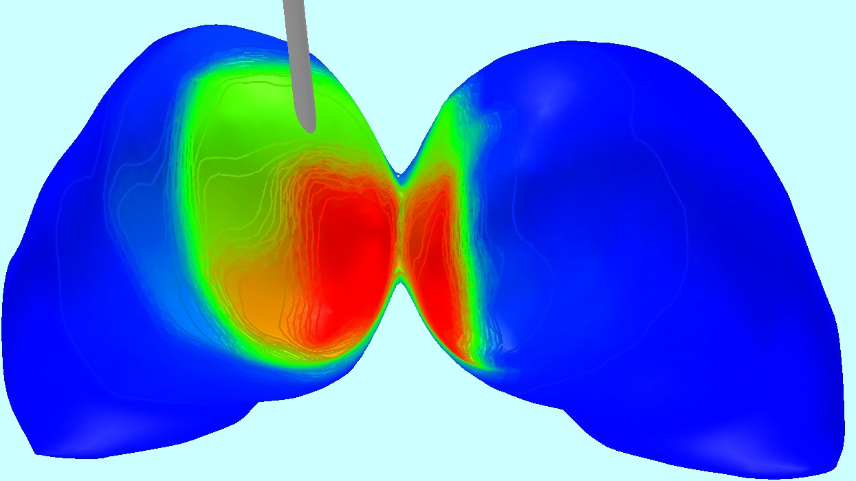
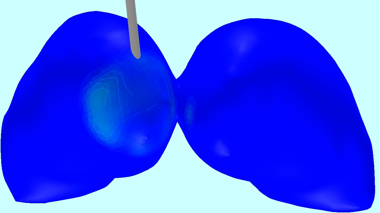
[HTML]ccffff	[HTML]ccffff	[HTML]ccffff	[HTML]ccffff	[HTML]ccffff	[HTML]ccffff	[HTML]ccffff
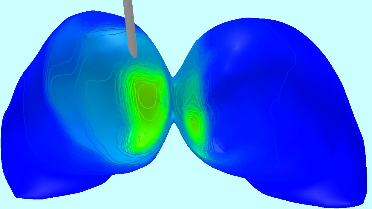
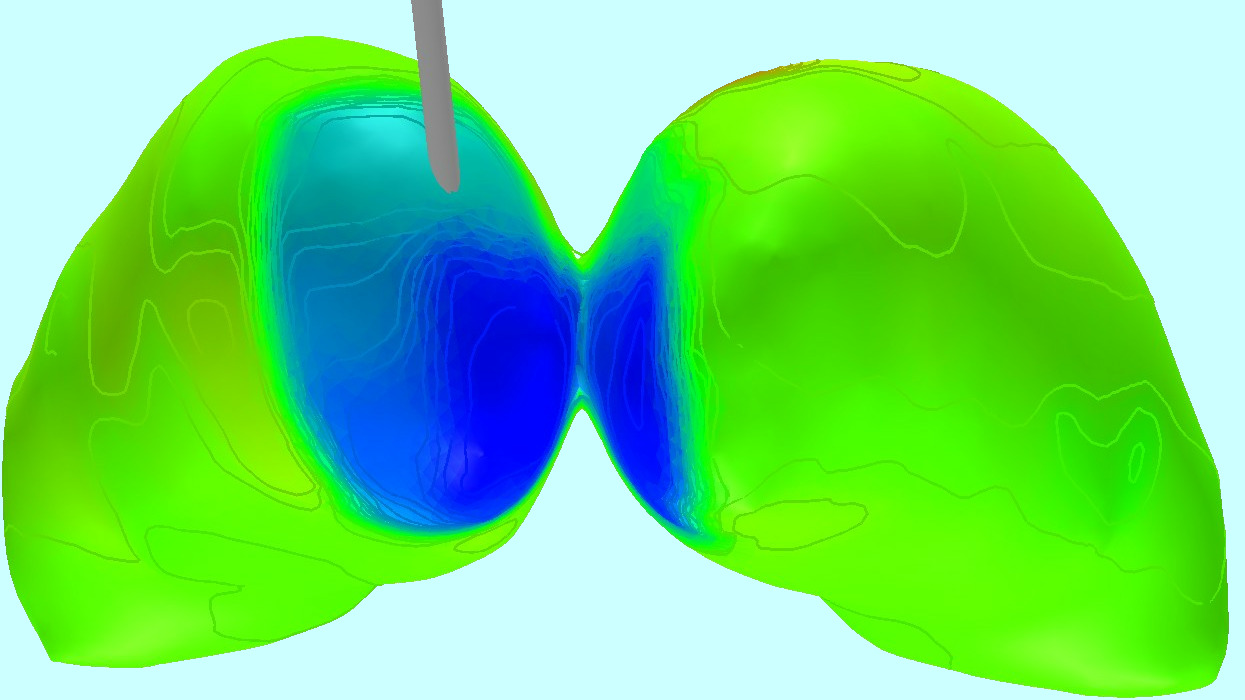
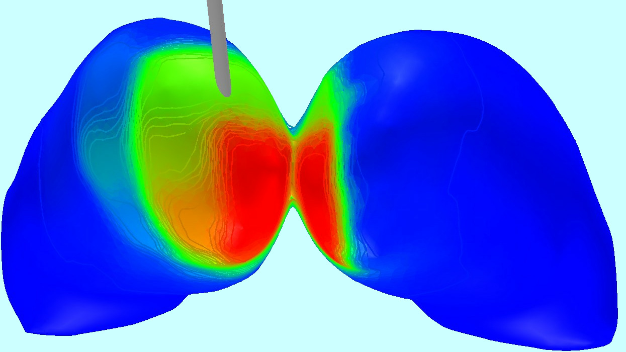
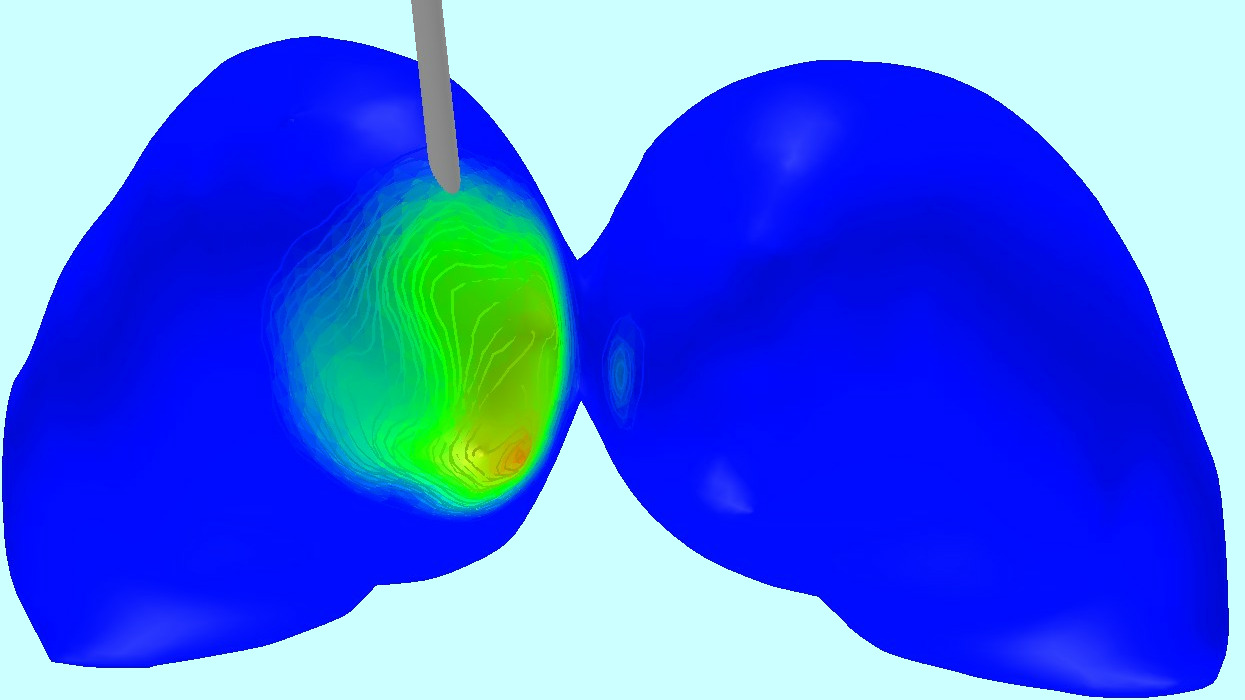
[HTML]ccffff L1L1(A), $\varepsilon\in[-160,0]$ dB   Perpendicular   Parallel	[HTML]ccffff	[HTML]ccffff	[HTML]ccffff	[HTML]ccffff	[HTML]ccffff	[HTML]ccffff
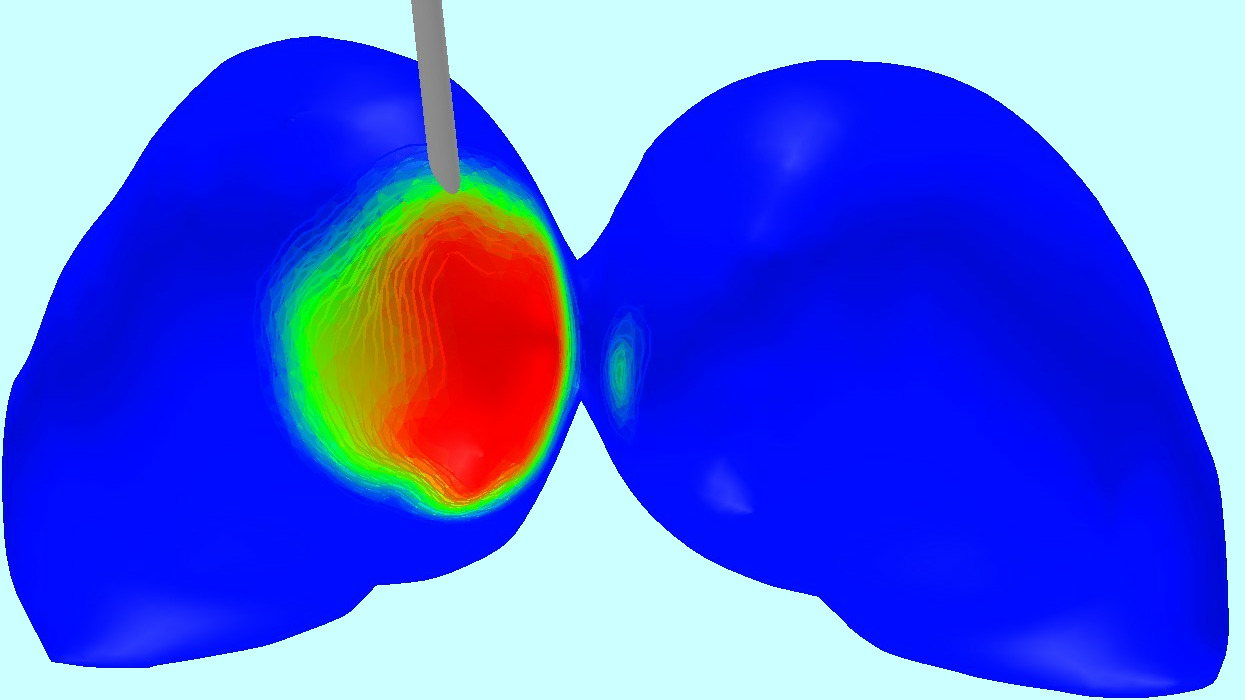
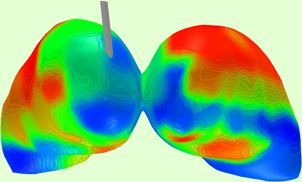
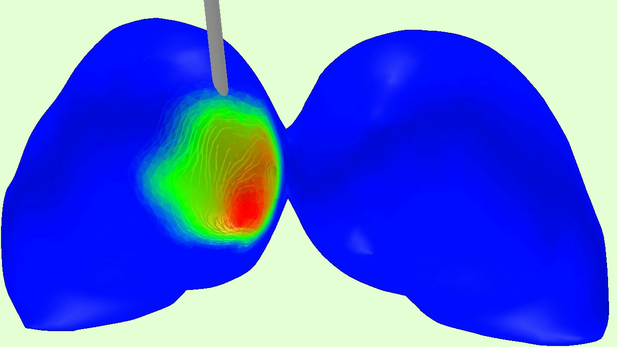
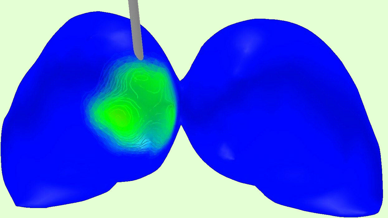
[HTML]e5ffd4	[HTML]e5ffd4	[HTML]e5ffd4	[HTML]e5ffd4	[HTML]e5ffd4	[HTML]e5ffd4	[HTML]e5ffd4
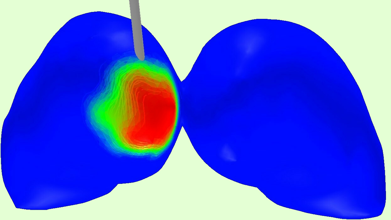
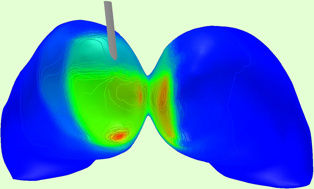
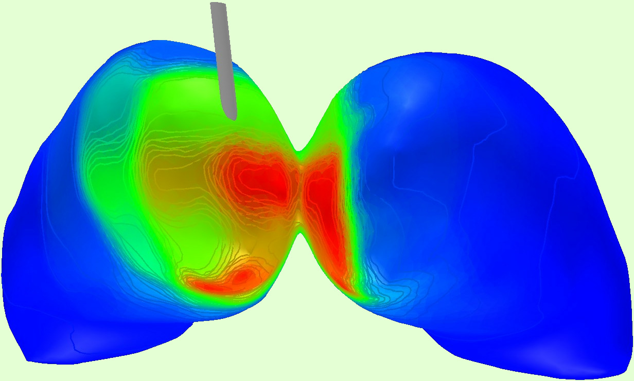
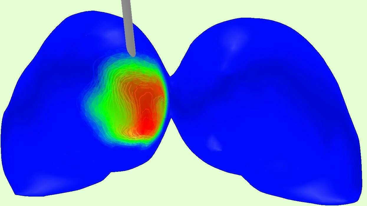
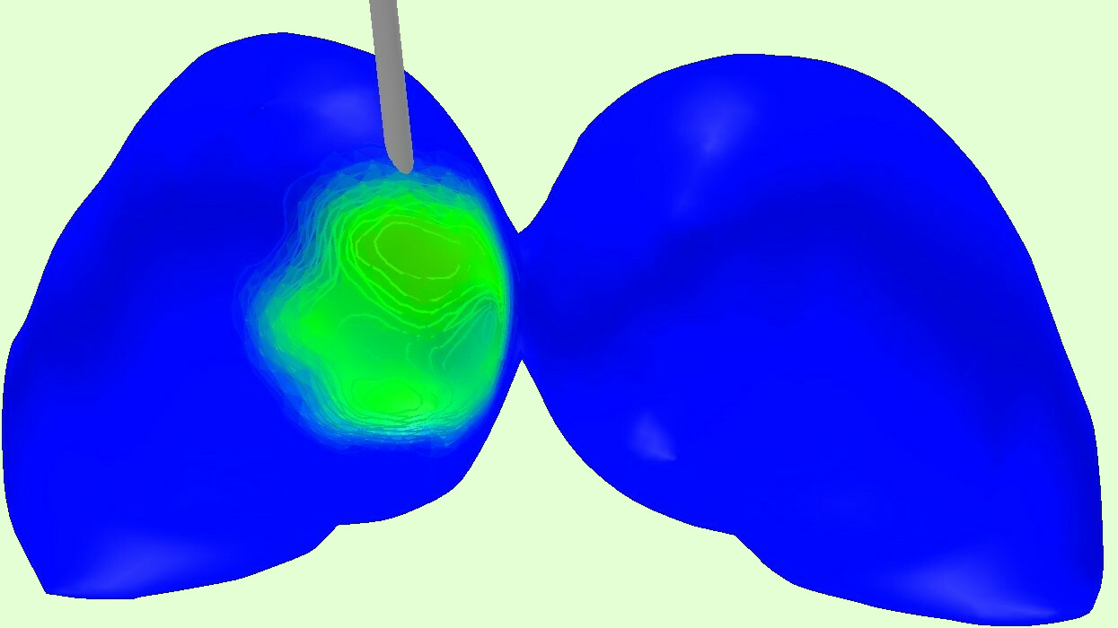
[HTML]e5ffd4 TLS, $\beta=[-50,40]$ dB   Perpendicular   Parallel	[HTML]e5ffd4	[HTML]e5ffd4	[HTML]e5ffd4	[HTML]e5ffd4	[HTML]e5ffd4	[HTML]e5ffd4

Figure 6: Volumetric optimization results for the 40-contact probe and noiseless lead fields. As compared to the results obtained with 8-contact probe the overall level of $\Theta$ is greater for L1L1(A), TLS and RP, while for L1L1(B) with limited dynamic range ($\varepsilon$ range) there is no clear increase.

3 Results

The applied algorithms generate distinct distributions of the variables $\Gamma$, $\Xi$, and $\Theta$, which can be differentiated based on how they are spatially organized across the target domain under the optimal electrode configurations for the 8- (Fig. 5) and 40-contact (Fig. 6) leads. The direction of the dipole current plays a key role in shaping electric field targeting. The anode–cathode pair exhibiting the strongest positive and negative values may activate electrodes located as close as $0.189\pm 0.009\,\text{mm}$ or as far as $6.375\pm 0.375\,\text{mm}$ apart across the lead. This effect becomes evident when comparing the corresponding distributions: in the parallel orientation, the targeting is highly concentrated near the tip of the probe, whereas the perpendicular orientation results in a broader spatial spread, with activity shifted medially relative to the lead.

The bipolar configurations obtained via RP yield the overall highest focused current density $\Gamma$; however, this comes at the expense of focality, as indicated by elevated nuisance current $\Xi$ and a reduced field ratio $\Theta$. This trade-off is understandable, as the multipolar configurations are designed to maximize the field ratio $\Theta$ subject to the constraint $\Gamma\geq\Gamma_{0}>0$, with $\Gamma_{0}=0.8\,\text{mA}$, thereby allowing activation of more than two contacts. In the noiseless setting, the L1L1(B) reconstructions with $\varepsilon\in[-10,0]\,\text{dB}$ yield slightly higher values of $\Gamma$ and $\Xi$, but exhibit a more moderate $\Theta$ compared to L1L1(A) with $\varepsilon\in[-160,0]\,\text{dB}$. Nonetheless, both L1L1(A) and L1L1(B) demonstrate superior nuisance current suppression relative to TLS and RP.

Figure 7 and Table 2 compare the noiseless and noisy ($\text{PSNR}=40\,\text{dB}$) results for $\Gamma$ and $\Theta$ obtained using L1L1(A) and L1L1(B) and LR-LF. The results suggest that, unlike L1L1(A), L1L1(B) is more robust to lead field noise, yielding similar outcomes in both settings. In contrast, L1L1(A), which uses a smaller lower bound for $\varepsilon$, tends to overfit the noiseless data. This leads to unrealistically high values of the field ratio $\Theta$: up to $27.07$ in the 8-contact configuration and as high as $536.05$ in the 40-contact case. However, in the presence of noise, the results produced by L1L1(A) fall within a similar range to those of L1L1(B), indicating that the overfitting is specific to the noiseless scenario.

Figure 8 further examines the noise sensitivity of RP, TLS, L1L1(A), and L1L1(B) for two specific target positions, illustrated in Figure 4, covering a sample of twenty different noise realizations for both PSNR 40 and 50 dB. The results demonstrate that in a noisy situation, L1L1(A) and L1L1(B) provide similar distributions for $\Gamma$ and $\Theta$, hence, also for $\Xi$. Compared to RP and TLS, the L1L1 approach seems to provide a somewhat elevated field ratio $\Theta$ with a difference that is only marginal or absent with PSNR 40 dB, but observable with PSNR 50 dB. Accordingly, the potential benefit of using L1L1 depends critically on the level of modeling uncertainty, and it vanishes when this uncertainty becomes excessive. Of the four optimization approaches tested, L1L1(B) provides the closest agreement between noiseless and noisy outcomes and proves particularly effective in maximizing the field ratio $\Theta$ in the presence of noise.

Table 2: The maximum values of the decision variable (DV) $\Theta$ (field ratio) found by L1L1(A) and L1L1(B) searches and the corresponding values of $\Gamma$ (focused current density) for the low-resolution lead field (LR-LF) and its target set (Figure 7) covering both parallel and perpendicular target orientations of the DBS lead in both noiseless and noisy (PSNR 40 dB) setting.

8-contacts		Multipolar
		L1L1(A), $\varepsilon\in[-160,0]$		L1L1(B), $\varepsilon\in[-10,0]$
DV	Orientation	No Noise	PSNR 40 dB	No Noise	PSNR 40 dB
$\Gamma$	Parallel	2.42	2.27	2.27	2.27
	Perpendicular	3.04	2.35	2.28	2.34
$\Theta$	Parallel	21.53	5.56	13.08	5.48
	Perpendicular	27.07	7.49	13.18	7.22

40-contacts		Multipolar
		L1L1(A), $\varepsilon\in[-160,0]$		L1L1(B), $\varepsilon\in[-10,0]$
DV	Orientation	No Noise	PSNR 40 dB	No Noise	PSNR 40 dB
$\Gamma$	Parallel	2.20	1.74	2.02	2.24
	Perpendicular	2.24	2.29	3.37	2.23
$\Theta$	Parallel	526.44	7.56	9.17	8.49
	Perpendicular	536.05	9.96	10.97	8.47

8-contact Electrode Configuration

 

Noiseless lead field

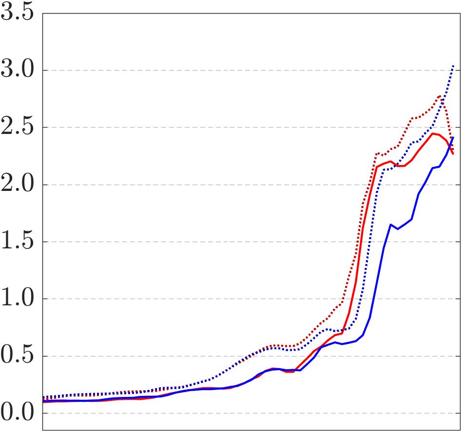
A1. Focus $\Gamma$ (A/m²)

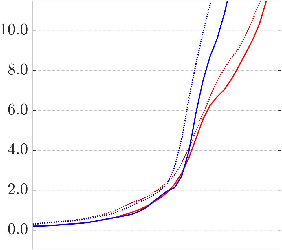
B1. Ratio $\Theta$ (rel.)

Noisy lead field

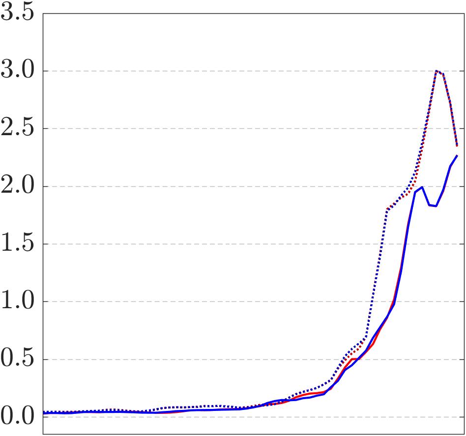
C1. Focus $\Gamma$ (A/m²)

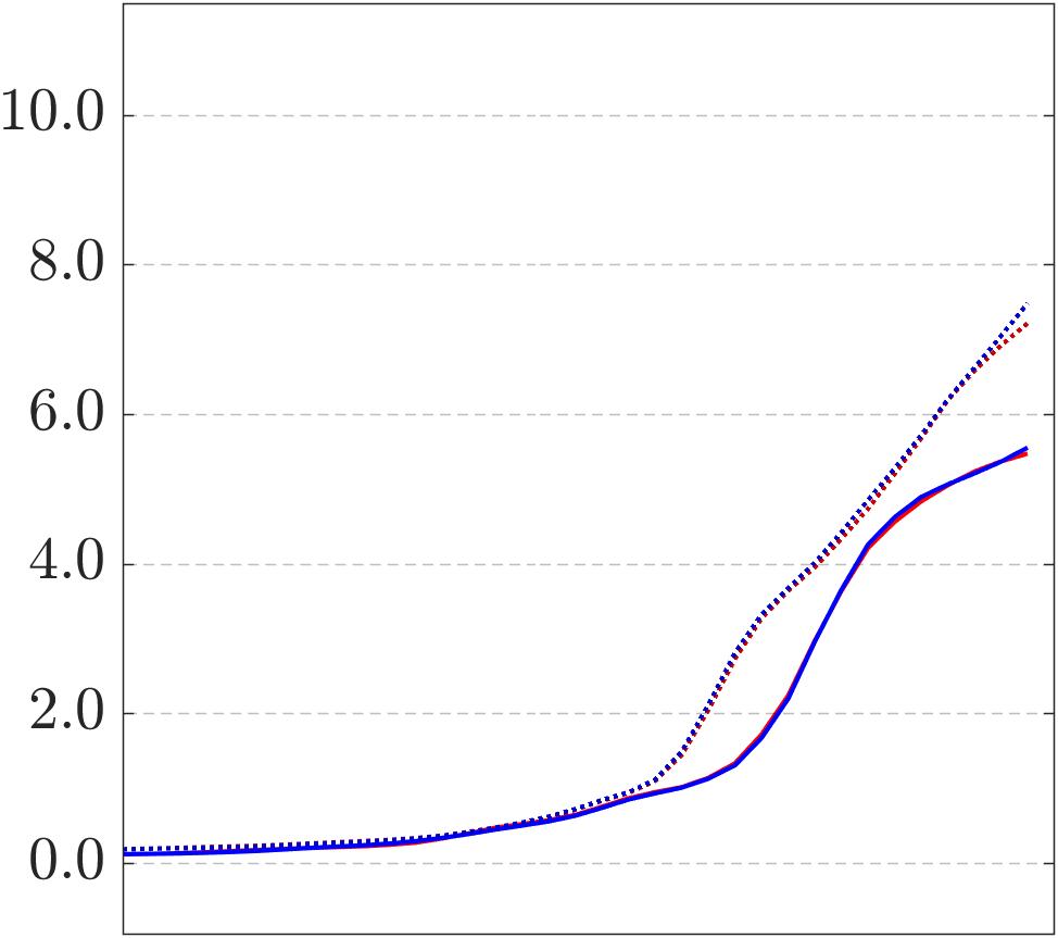
D1. Ratio $\Theta$ (rel.)

40-contact Electrode Configuration

 

Noiseless lead field

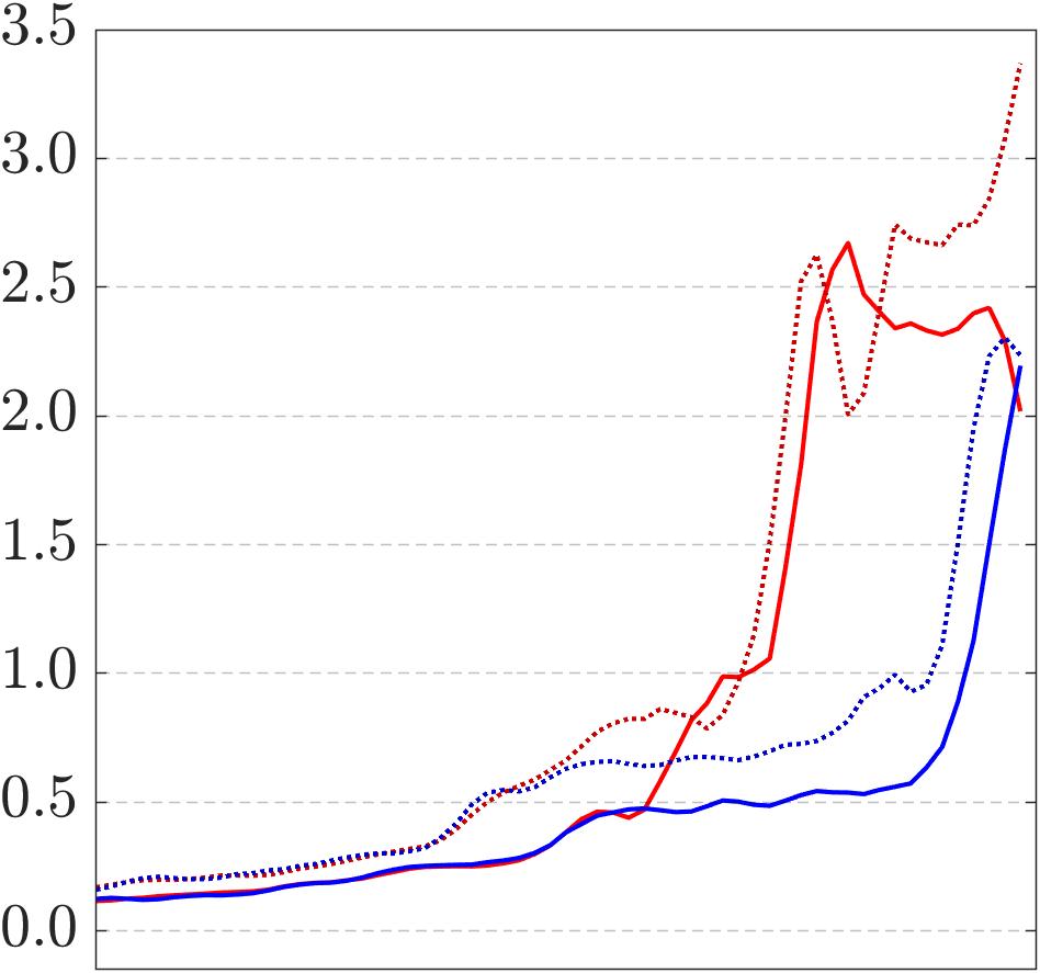
A2. Focus $\Gamma$ (A/m²)

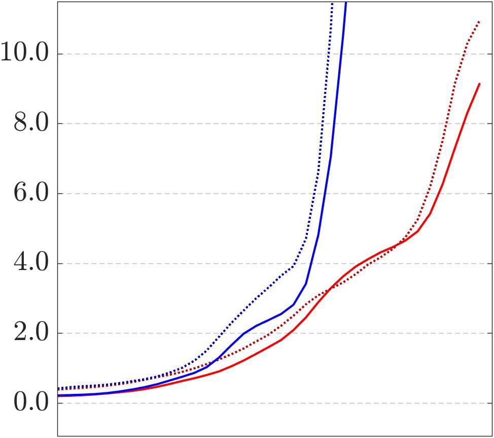
B2. Ratio $\Theta$ (rel.)

Noisy lead field

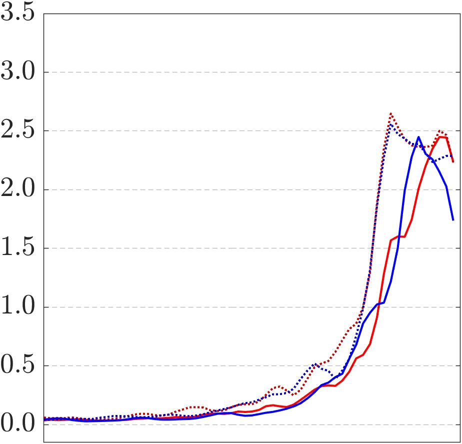
C2. Focus $\Gamma$ (A/m²)

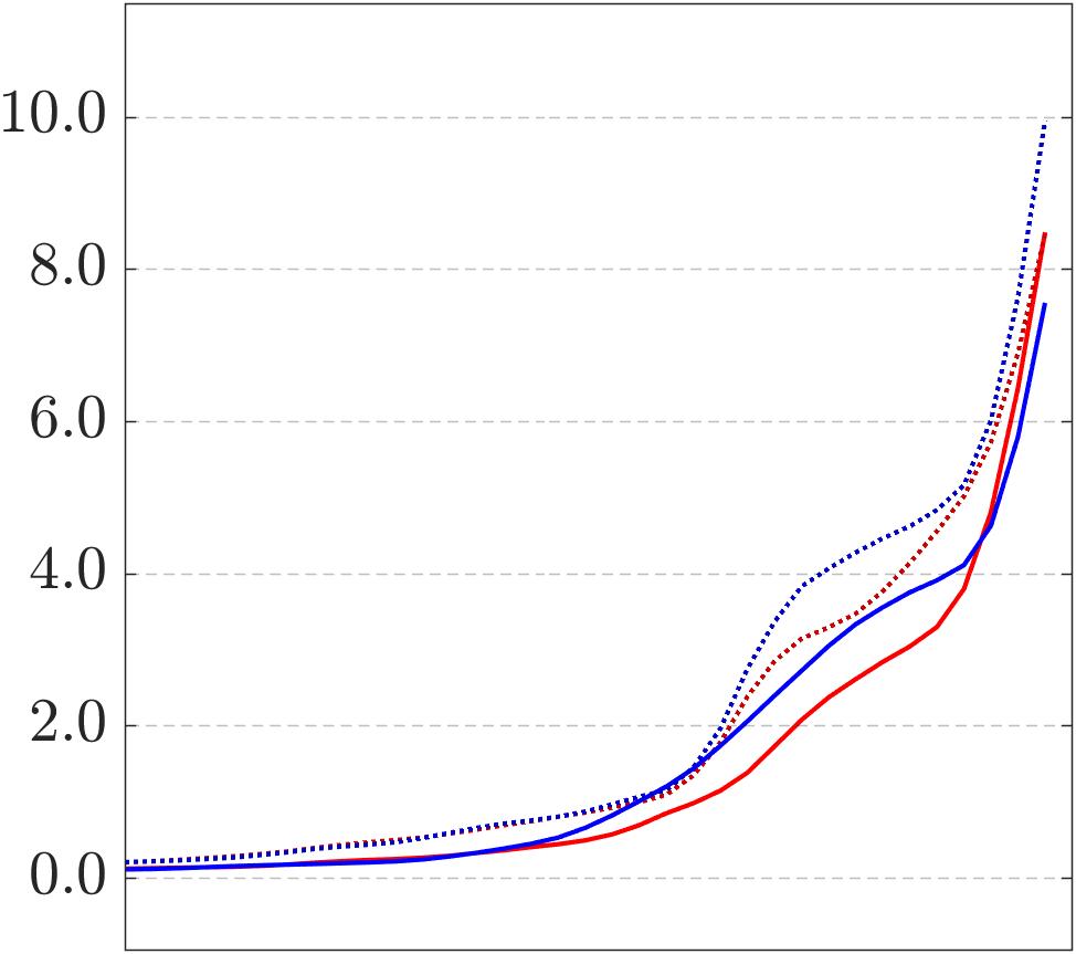
D2. Ratio $\Theta$ (rel.)

Figure 7: Performance of L1L1(A) and L1L1(B) for optimizing the field ratio $\Theta$ subject to criterion $\Gamma\geq\Gamma_{0}$ with noiseless and noisy (PSNR 40 dB) lead field. L1L1(A) and L1L1(B) suppress the nuisance current density $\Xi$ pattern using two different dynamic ranges, namely, $\varepsilon\in[-160,0]$ (blue) and $\varepsilon\in[-10,0]$ (red), respectively. The results are sub-grouped by the direction of the current dipole, whether its alignment is parallel (solid line) or perpendicular (dotted line) with the applied lead. The degrees of freedom have been sorted according to ascending field ratio $\Theta$. The results show that the overly optimistic dynamic range applied in L1L1(A) results in very high field values of $\Theta$ in the noiseless case, which are, however, absent in the noisy one. In contrast, L1L1(B) is only marginally affected by the noise due to more realistic assumption of the maximum obtainable dynamic range under uncertainty.

8-contact Electrode Configuration

 

Parallel

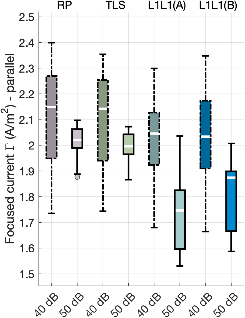
Focus $\Gamma$ (A/m²)

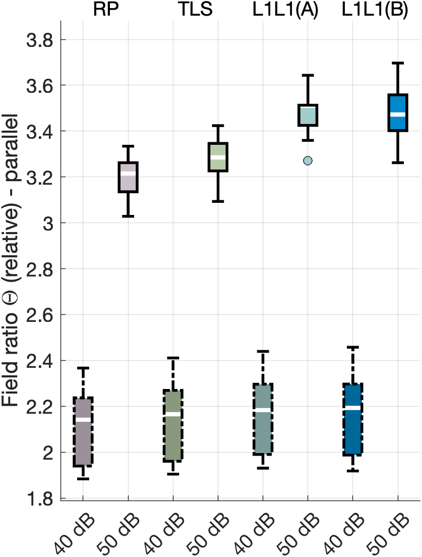
Ratio $\Theta$ (rel.)

Perpendicular

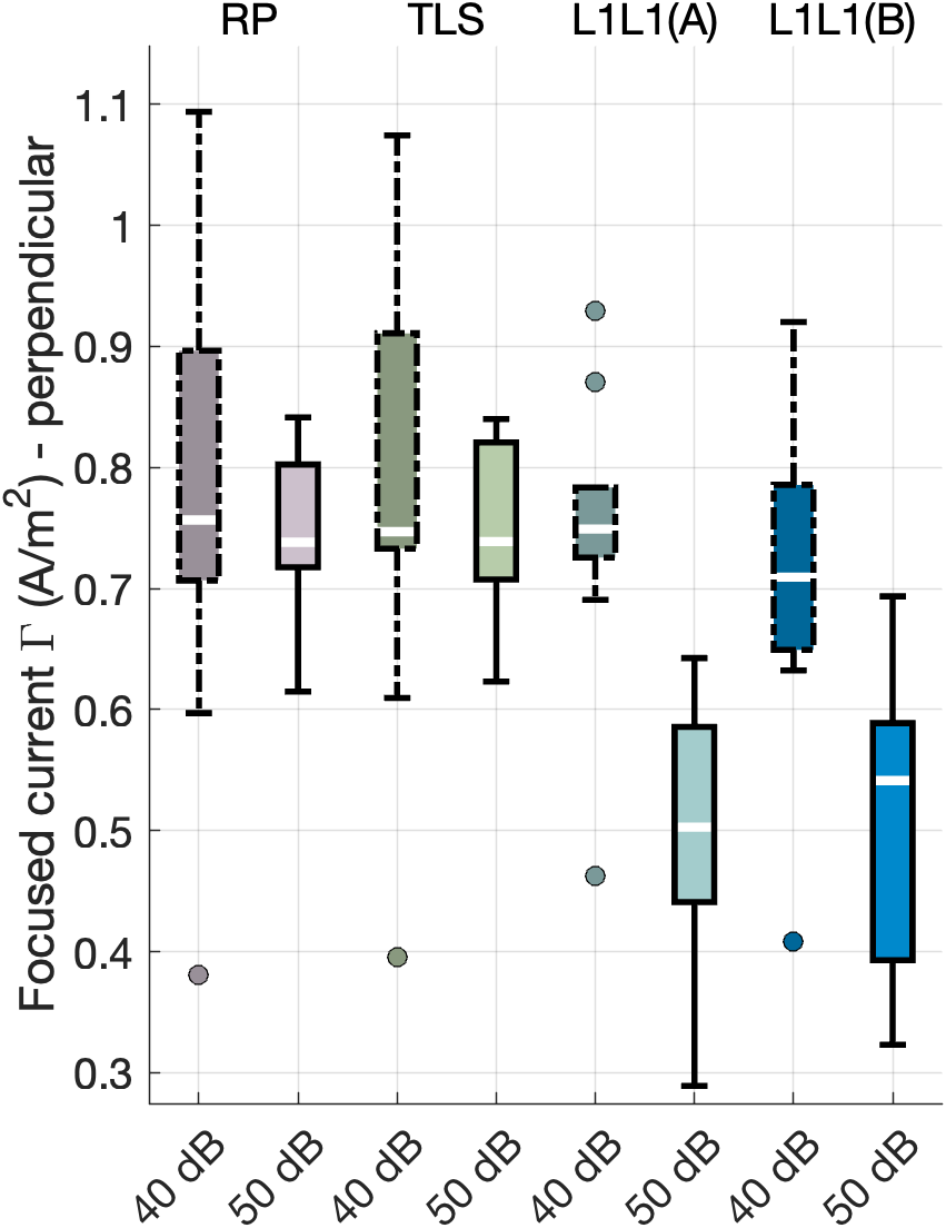
Focus $\Gamma$ (A/m²)

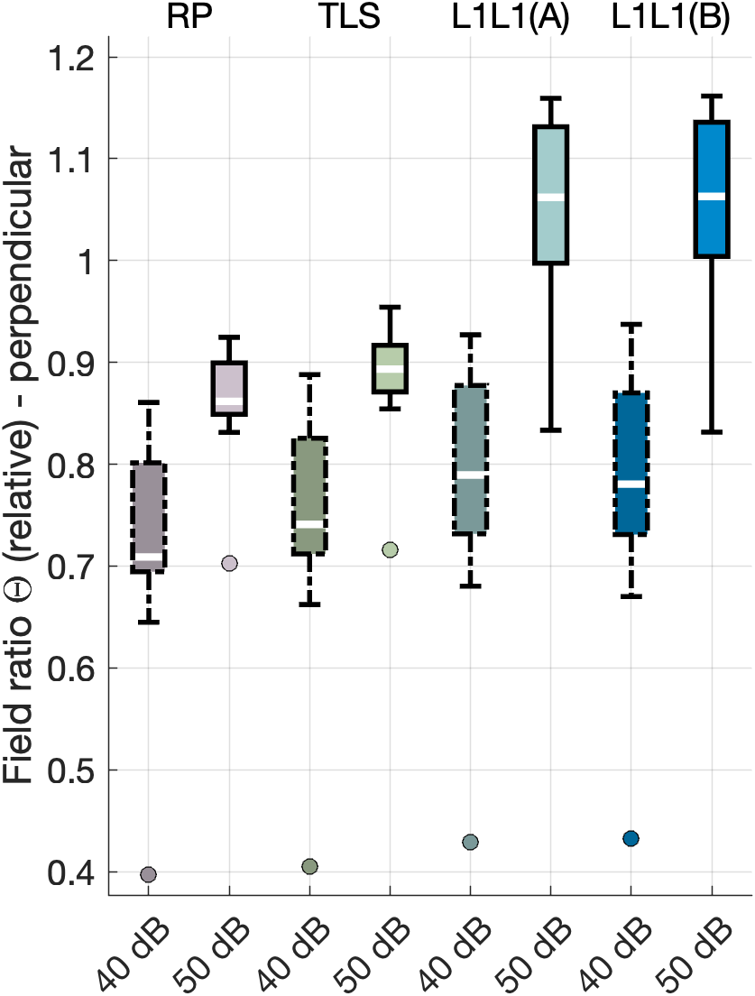
Ratio $\Theta$ (rel.)

Target (I)

Parallel

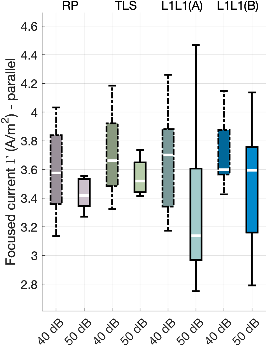
Focus $\Gamma$ (A/m²)

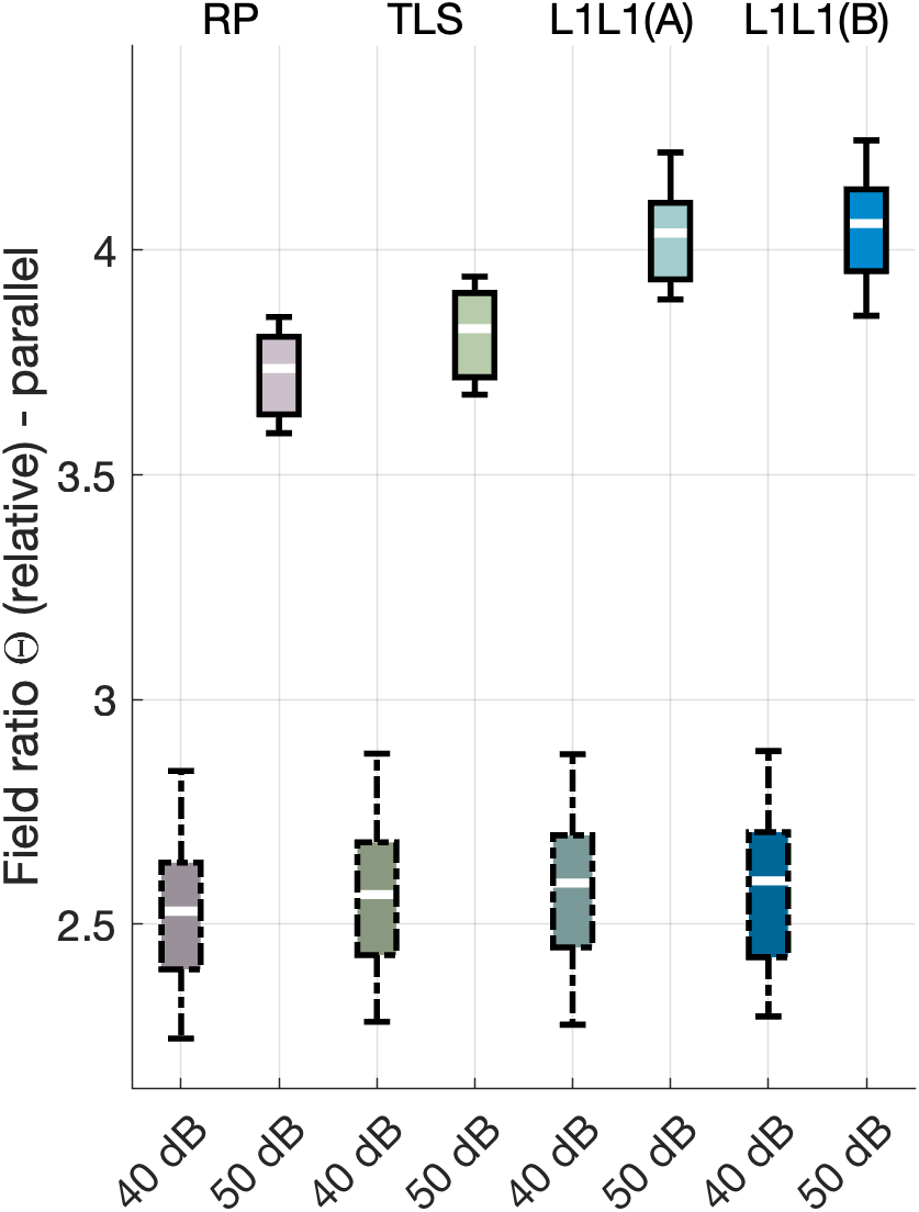
Ratio $\Theta$ (rel.)

Perpendicular

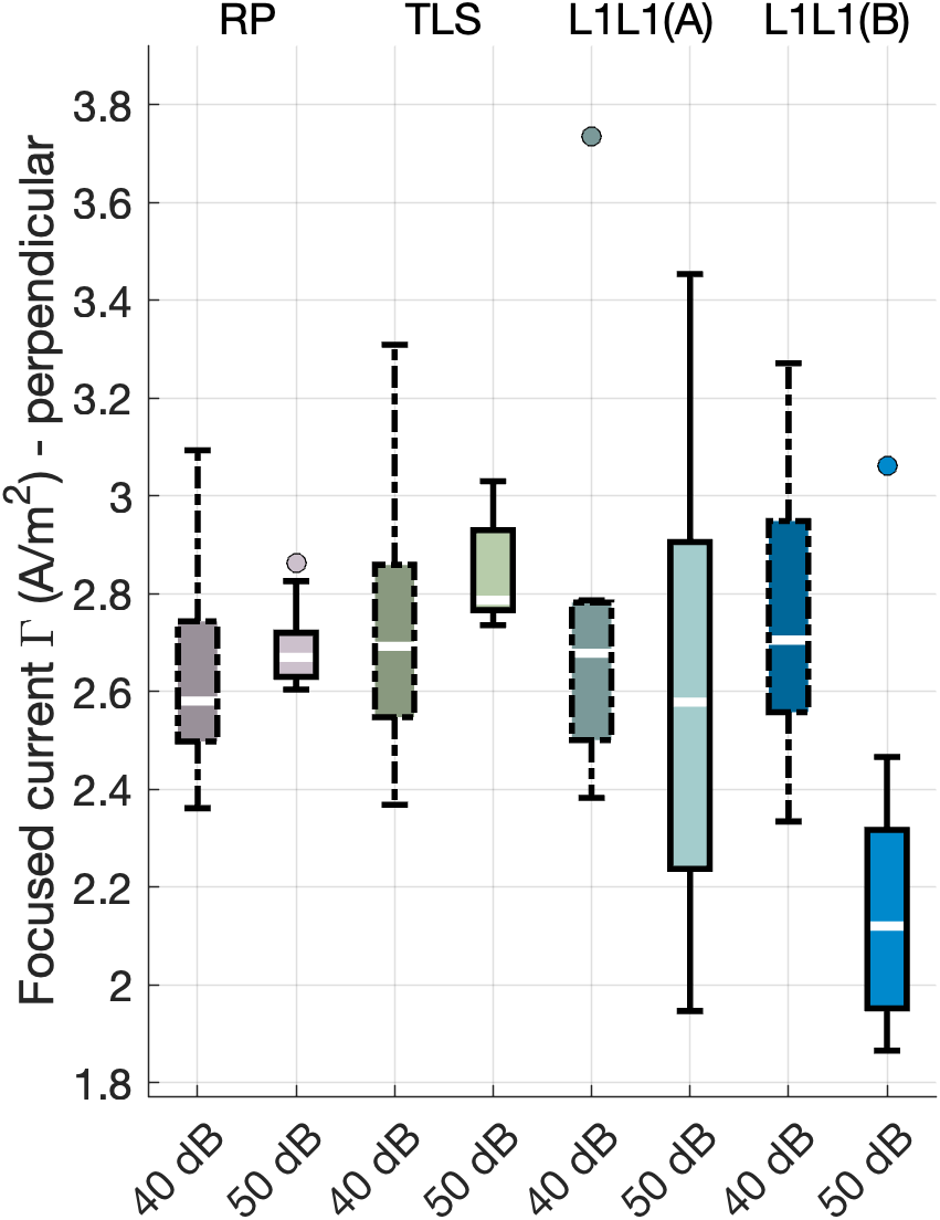
Focus $\Gamma$ (A/m²)

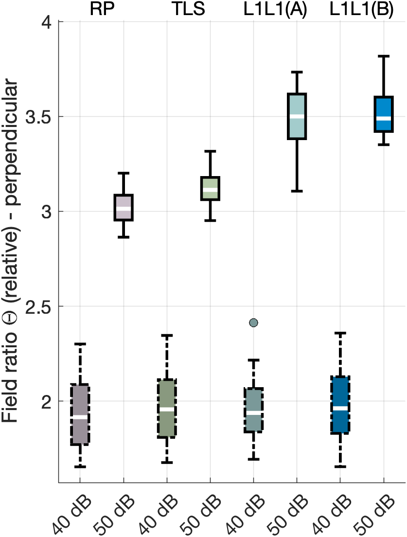
Ratio $\Theta$ (rel.)

Target (II)

40-contact Electrode Configuration

 

Parallel

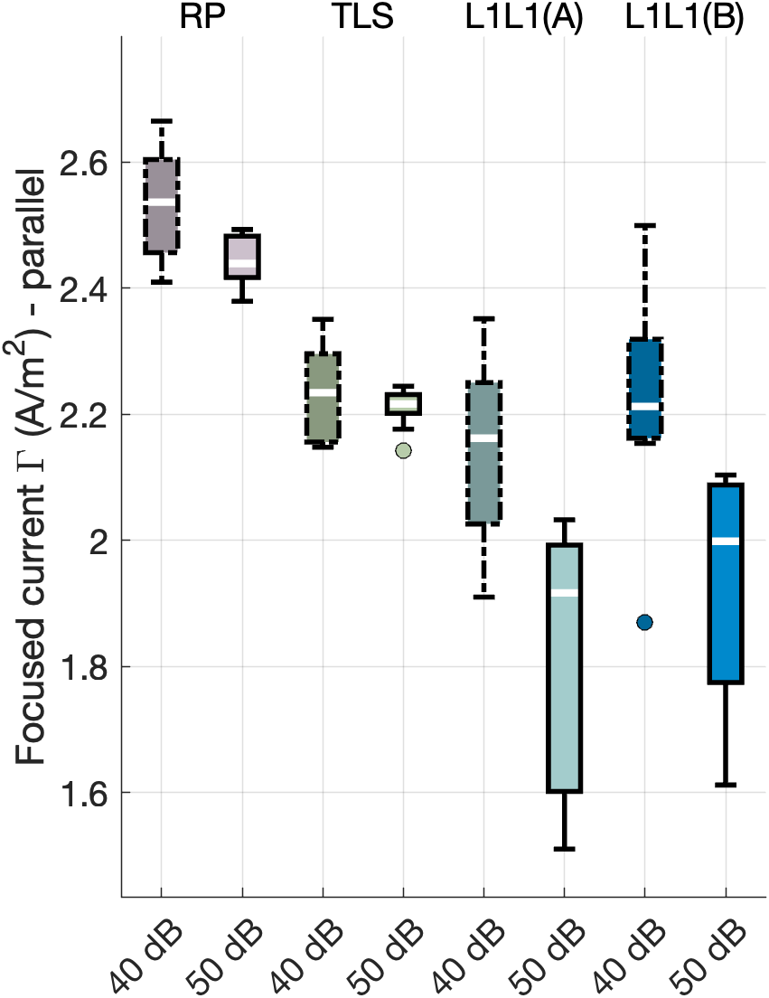
Focus $\Gamma$ (A/m²)

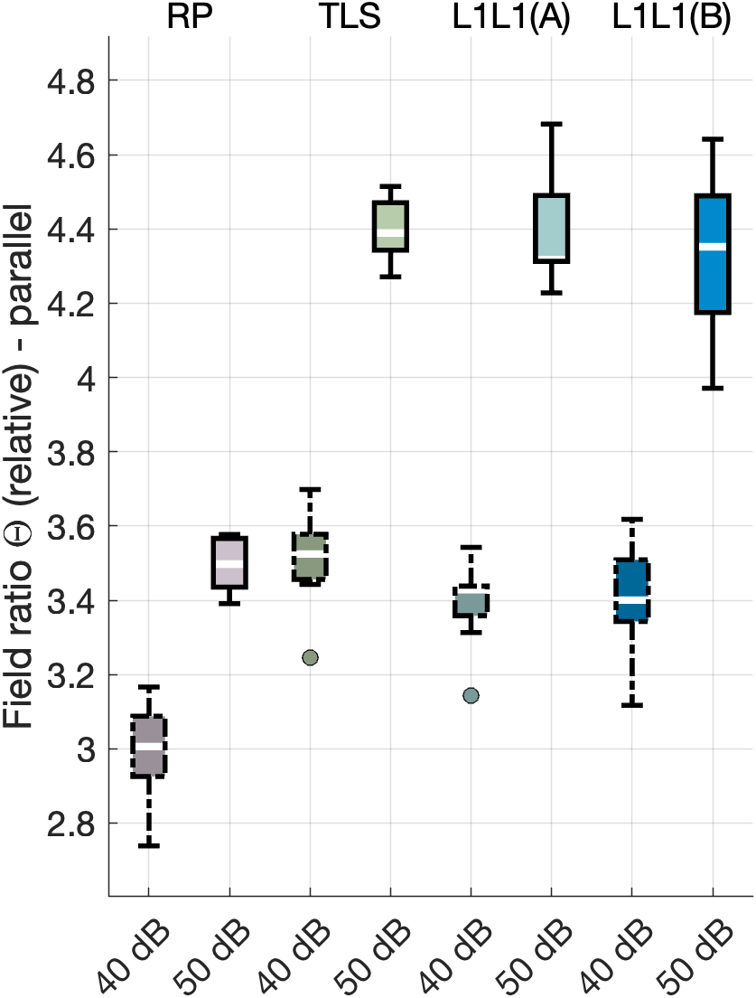
Ratio $\Theta$ (rel.)

Perpendicular

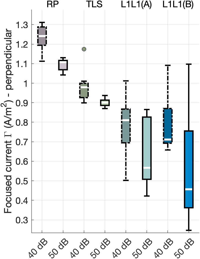
Focus $\Gamma$ (A/m²)

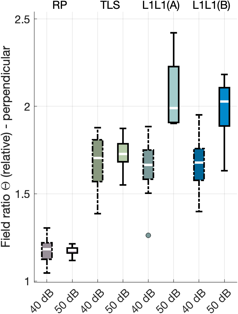
Ratio $\Theta$ (rel.)

Target (I)

Parallel

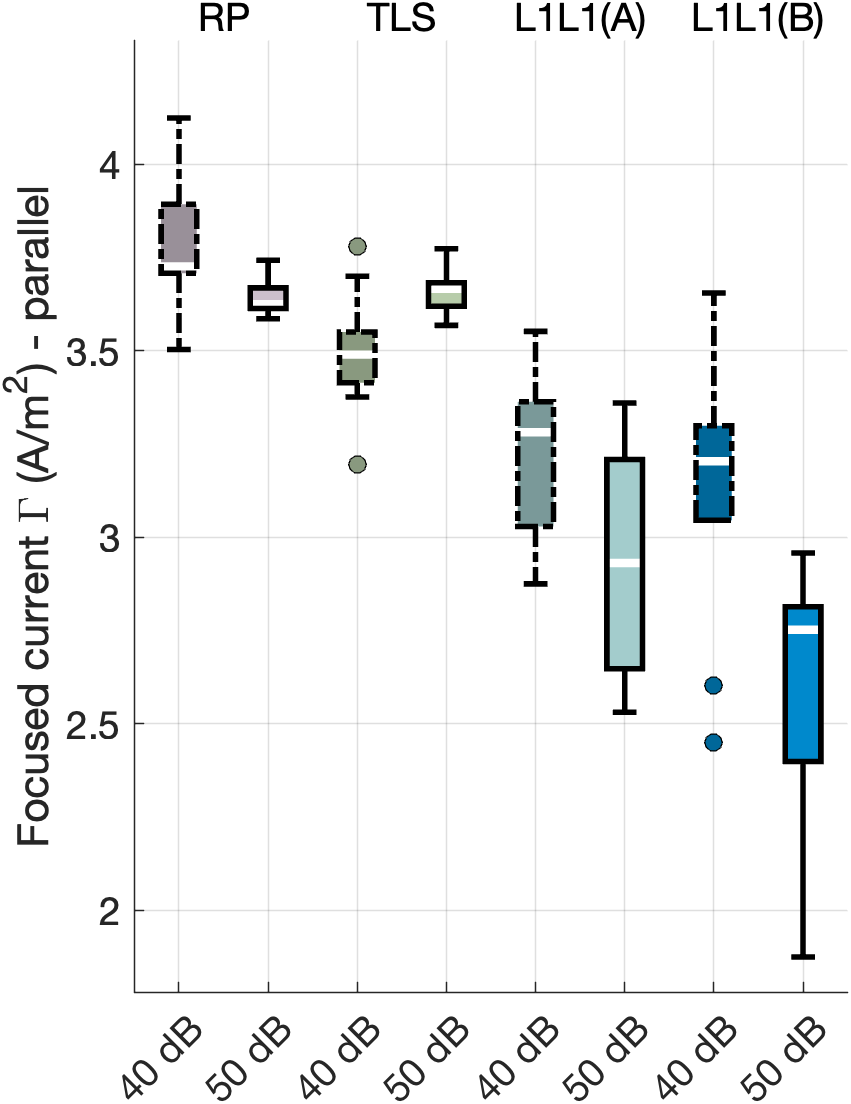
Focus $\Gamma$ (A/m²)

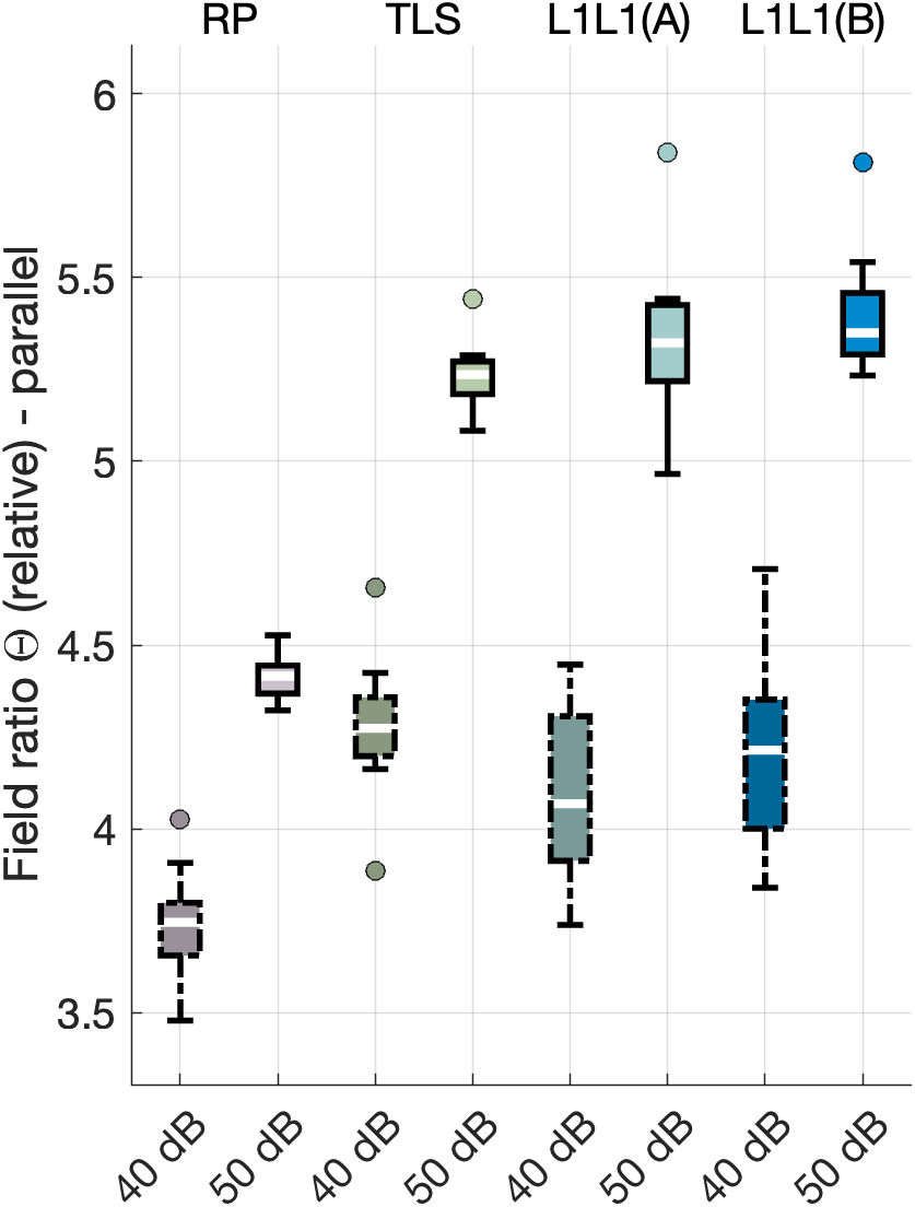
Ratio $\Theta$ (rel.)

Perpendicular

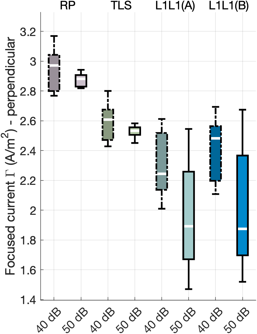
Focus $\Gamma$ (A/m²)

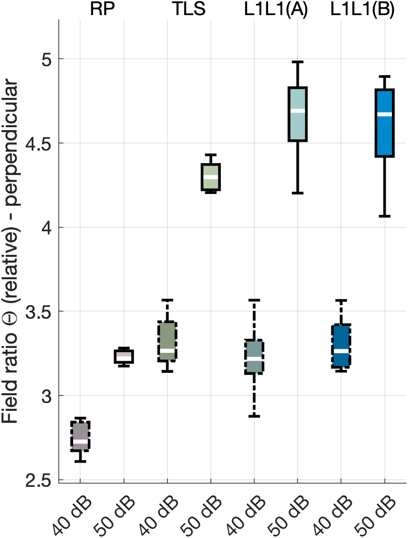
Ratio $\Theta$ (rel.)

Target (II)

Figure 8: Boxplots showing the focused current density $\Gamma$ and field ratio $\Theta$ obtained with a noise-corrupted HR-LF and the 8-contact electrode configuration for test targets (I) and (II). The optimizers have been found through RP, TLS, L1L1(A), and L1L1(B) search. Each bar collates a sample of twenty decision variable values corresponding to optimizers obtained with as many independent lead field noise realizations (PSNR 40 or 50 dB). The box shows the interquartile range (IQR) between the first quantile $Q1$ and the third one $Q3$, with a horizontal line at the median. The whiskers extend from the edges of the box to the smallest and largest values within $[Q1-1.5\times\text{IQR},Q3+1.5\times\text{IQR}]$, where $\text{IQR}=Q3-Q1$. Data points outside this range are considered outliers and are plotted individually as markers. The results obtained with L1L1(A) and L1L1(B) demonstrate a comparable sensitivity under lead field noise, suggesting that the limited dynamic range of L1L1(B) does not downgrade the L1L1 method’s performance in situations involving uncertainty. Furthermore, both L1L1(A) and L1L1(B) find an overall elevated field ratio compared to RP and TLS with the greater PSNR level 50 dB, which allows for an improved +10 dB dynamic range for the optimization algorithm as compared to PSNR 40 dB.

4 Discussion

This study explores the application of the recently introduced metaheuristic L1L1 method [32], to optimize the current patterns for DBS leads. The core focus lies in L1L1’s capacity to incorporate a priori uncertainty through an explicit constraint, offering a notable advantage over traditional approaches, which often fail to account for such variability [37, 38, 36, 59]. Specifically, we define the uncertainty through a threshold on the nuisance current density, which is determined by the relative attenuation of the lead field with respect to a target site. This attenuation is quantified in decibels and corresponds to typical falloff patterns observed in VTA. By reducing the dependence on conventional parameter tuning methods, such as trial-and-error [60, 61], this approach paves the way for more sophisticated techniques to make more informed decisions, even in the presence of inherent uncertainties in DBS settings and simulations [62, 63, 64, 65].

Optimization was carried out using three parameters: the focused current density $\Gamma$, the nuisance current density $\Xi$, and field ratio $\Theta=\Gamma/\Xi$. To assess robustness and focality under uncertainty, the recently introduced L1L1 method was applied in two variants, L1L1(A) and L1L1(B), differing in the range of the nuisance current threshold $\varepsilon$, which reflects varying levels of a priori modeling uncertainty. Specifically, L1L1(B) constrains $\varepsilon$ to the interval $[-10,0]$ dB, accounting for higher uncertainty, whereas L1L1(A) utilizes a broader range $[-160,0]$ dB. For comparison, the Reciprocity Principle (RP) and Tikhonov-Regularized Least Squares (TLS) methods were included as reference approaches.

The results reveal that the spatial distributions of $\Gamma$, $\Xi$, and $\Theta$ are strongly influenced by both the optimization method and the orientation of the dipole current. Parallel configurations resulted in highly localized activation near the tip of the lead, whereas perpendicular configurations yielded a broader, medially shifted targeting. A comparative analysis across varying noise levels demonstrated that L1L1 methods consistently outperformed RP and TLS in maintaining higher and more stable values of $\Theta$, especially at higher PSNR values.

In noiseless conditions, solutions obtained with a low nuisance threshold $\varepsilon\in[-160,0]\,\text{dB}$, as in L1L1(A), often exhibited unrealistically high field ratio values $\Theta$, sometimes up to fifty times greater than those derived using the more conservative threshold $\varepsilon\in[-10,0]\,\text{dB}$ in L1L1(B). This tendency suggests overfitting when the model is not constrained by uncertainty. Introducing this noise regularized the solution space, preventing the algorithm from converging to over-idealized solutions that mirrored the original model structure. These findings underscore the significance of explicitly modeling uncertainty and justify the constraint imposed on the nuisance current in L1L1(B), which leads to more realistic and generalizable solutions. Overall, these observations highlight the potential of L1L1(B) as a robust and uncertainty-aware optimization strategy for dDBS lead configuration.

The estimates for the set $\mathcal{V}_{\delta}$, where the lead field amplitude attenuates by a factor $\delta$ for $\delta\in[-40,-10]$ dB, align closely with established knowledge regarding VTA. Specifically, for $\delta\approx-40\,\text{dB}$, our model predicts attenuation within a spatial region consistent with a VTA radius of approximately 4.0 mm, in line with the findings of Butson’s [33] and McIntyre’s [20]. This agreement suggests that the noise levels used, with PSNR values of 40 dB and 50 dB, represent reasonable bounds for physiological uncertainty. At 40 dB, the dynamic range of $\Theta$ is determined by the maximum lead field attenuation within the VTA, while 50 dB further supports the assumption that each position within the VTA can be independently and coherently targeted. In this context, the L1L1 method, particularly L1L1(B), demonstrated superior targeting capabilities compared to RP and TLS, especially under noisy conditions.

When comparing the electrode configurations, increasing the number of contact points generally enhances both adaptability and control over the resulting electric field. This improvement is driven by several factors, including reduced distances between electrodes and target locations within the lead field matrix, better alignment of the induced electric field with the target current direction, and a greater capacity for flexible fitting due to the increased number of degrees of freedom.

The findings of this study provide a proof-of-concept for integrating a priori uncertainty modeling into numerically simulated dDBS optimization. When relevant sources of uncertainty, such as anatomical variability, conductivity inhomogeneities, or lead placement deviations, are known or can be estimated, the L1L1 method might be employed to improve the focality and directionality of stimulation, enabling more selective targeting of desired structures while reducing activation in surrounding regions. In clinical practice, such improvements might lead to more personalized and effective treatment strategies, enhancing therapeutic precision, and minimizing side effects [10].

4.1 Limitations and Future Work

While the current uncertainty modeling strategy provides a principled framework for constraining the optimization based on lead field attenuation, it also has several limitations. First, the threshold values used to define acceptable nuisance current levels are heuristic and may not fully capture the complexity of individual patient anatomies or tissue conductivities. This simplification assumes spatial uniformity in attenuation, which may not hold, for example, in the presence of anisotropic or heterogeneous tissue properties [44, 66]. Additionally, the approach relies on a static surrogate model of the VTA and does not directly incorporate a probabilistic model of uncertainty [62], which would allow for a more comprehensive treatment of variability. Potential alternative surrogate approaches exist, such as, threshold-based curve fitting [67], artificial neural networks [68], and statistical emulators such as Gaussian process classifiers [69, 70], which approach VTA in different ways.

Compared to the reference methods of this study, the L1L1 method is also slightly more demanding in terms of computing time. However, the increase is not significant and does not limit its practical use.

Other mathematical optimization techniques, such as Tikhonov (TLS) [38, 37], may offer promising alternatives alongside the L1L1 method for further refining the a priori uncertainty modeling adopted in this study. A logical direction for future research is the development of a posteriori models, where the current approach could be validated in more advanced experimental or clinical settings. This would enable a deeper understanding of the potential hyperparameter realizations in real-world applications. Translating these computational findings into clinical practice will require rigorous validation through empirical testing and clinical trials.

An ongoing work is the inclusion of more patient-specific anatomical and physiological data, e.g., a thalamic segmentation, to ensure more personalized and accurate stimulation strategies. Therefore, we explore the use of FE-based discretizations incorporating thalamic subdivisions via boundary-fitted multicompartment FE meshing approach and a complete electrode model, as utilized in this study.

5 Conclusions

This study represents an advancement in optimizing the volumetric current fields for DBS by leveraging the metaheuristic L1L1 method. Previous studies on contact selection have used convex optimization and patient-specific models to determine optimal stimulation settings. These methods perform well when all input parameters are fixed. However, they do not account for uncertainties in factors such as patient anatomy, lead placement, and tissue properties, which often vary in clinical practice. In principle, our L1L1-based method can address these uncertainties. Its main advantage is the ability to target the desired area while avoiding overfitting to noisy data.

Our findings demonstrate the method’s ability to refine electrode contact point configurations under varying levels of a priori lead field uncertainty. By achieving relatively high field ratios with a carefully chosen $\varepsilon$ value, the L1L1 method shows promise in enhancing the precision and effectiveness of DBS stimulation within uncertainty constraints. This, in turn, has the potential to improve individualized stimulation outcomes. An ongoing work is to integrate patient-specific data, such as thalamic segmentation, to improve stimulation accuracy. This involves using boundary-fitted multicompartment FE meshes and a complete electrode model, as in this study.

6 Conflict of Interest

The authors certify that this study is a result of purely academic, open, and independent research. They have no affiliations with or involvement in any organization or entity with a financial interest or non-financial interest, such as personal or professional relationships, affiliations, knowledge, or beliefs in the subject matter or materials discussed in this manuscript.

7 Author Contributions

FGP: Conceptualization, Formal analysis, Investigation, Methodology, Software, Visualization, Writing—original draft. AL: Conceptualization, Data curation, Investigation, Methodology, Project administration, Writing—original draft. MS: Formal analysis, Supervision, Validation, Writing—review & editing. SP: Conceptualization, Formal analysis, Funding acquisition, Investigation, Methodology, Project administration, Resources, Software, Supervision, Validation, Visualization, Writing—review & editing.

8 Funding

FGP, MS, and SP were supported by the Research Council of Finland through the Center of Excellence in Inverse Modelling and Imaging 2018–2025 (353089); the researcher exchange (DAAD) project ”Non-invasively reconstructing and inhibiting activity in focal epilepsy” (354976, 367453); the ERA PerEpi project (344712), and Flagship of Advanced Mathematics for Sensing, Imaging and Modelling (FAME) (359185, 359198)

9 Acknowledgments

The authors would like to thank Prof. Dr. rer. nat. Carsten H. Wolters, researchers and clinicians from the Institute for Biomagnetism and Biosignalanalysis (IBB), and the PerEpi consortium for their continuous support, discussions, and feedback regarding non-invasive brain stimulation topics, regression analysis, and the seminars prepared during the elaboration of this study.

Appendix A Mathematical Optimization Scheme

We consider a weighted optimization scheme governed by the linear system

$${\bf L}{\bf y}={\bf x},$$ (1)

where $\mathbf{y}\in\mathbb{R}^{K}$ is the current pattern to be optimized, $\mathbf{x}\in\mathbb{R}^{N}$ is the discretized volume current density vector, and $\mathbf{L}\in\mathbb{R}^{N\times K}$ is the lead field matrix defining a linear forward mapping from current patterns to the resulting current density field. This system is derived by component-wise splitting of the full lead field matrix $\hat{\mathbf{L}}\in\mathbb{R}^{N\times K}$ and the full current field $\hat{\mathbf{x}}\in\mathbb{R}^{N}$, such that

$$\hat{\mathbf{L}}=\begin{pmatrix}\hat{\mathbf{L}}_{1}\\ \hat{\mathbf{L}}_{2}\end{pmatrix},\quad\hat{\mathbf{x}}=\begin{pmatrix}\hat{\mathbf{x}}_{1}\\ \mathbf{0}\end{pmatrix},$$ (2)

where $\hat{\mathbf{x}}_{1}\in\mathbb{R}^{N_{1}}$ corresponds to the target region of interest and the zero component enforces field suppression elsewhere. The reduced system (1) is then defined by

$$\mathbf{L}=\begin{pmatrix}\mathbf{L}_{1}\\ \mathbf{L}_{2}\end{pmatrix}=\begin{pmatrix}\mathbf{P}\hat{\mathbf{L}}_{1}\\ \hat{\mathbf{L}}_{2}\end{pmatrix},\quad\mathbf{x}=\begin{pmatrix}\mathbf{x}_{1}\\ \mathbf{0}\end{pmatrix}=\begin{pmatrix}\mathbf{P}\hat{\mathbf{x}}_{1}\\ \mathbf{0}\end{pmatrix}.$$ (3)

Here, $\mathbf{P}\in\mathbb{R}^{N_{1}\times N_{1}}$ is a projection matrix that projects vectors onto the direction of $\hat{\mathbf{x}}_{1}$, which is assumed to have fixed direction. This projection ensures that alignment between the induced and target fields is measured only along the direction of interest. In this formulation, the upper part $\hat{\mathbf{L}}_{1}\mathbf{y}=\hat{\mathbf{x}}_{1}$ defines the focused current field in the target region, while the lower part $\hat{\mathbf{L}}_{2}\mathbf{y}=\mathbf{0}$ defines the nuisance field to be suppressed outside the region of interest.

A.1 L1-norm regularized L1-norm fitting

The general form of the L1-norm regularized L1-norm fitting (L1L1) method described by Galaz Prieto et. al [32, 57] is an optimization problem designed to minimize a linear objective function of continuous real variables subject to linear constraints. The optimization problem needs to find the best matching between ${\bf y}$, and the focused field via ${\bf L}{\bf y}={\bf x}$. The task is

$$\underset{y}{\textrm{minimize}} \quad\left\|\begin{pmatrix}{\bf L}_{1}{\bf y}-{\bf x}_{1}\\ \Psi_{\varepsilon}[\nu^{-1}{\bf L}_{2}{\bf y}]\end{pmatrix}\right\|_{1}+{\alpha}\zeta\|{\bf y}\|_{1},$$ (4)

subject to $$\quad{\bf y}\preceq\gamma{\bf 1},$$ (5)

$$\quad\|{\bf y}\|_{1}\leq\mu,$$ (6)

$$\quad\sum_{\ell=1}^{K}y_{\ell}=0,\,\quad\ell=1,\ldots,K.$$ (7)

The linear constraint 5 implies that the individual current injection for each $\ell$-th electrode is limited to a $\Gamma$ value; constraint 6 implies the total current injection flowing through the system is within a safety $\mu$-value limit; and constraint 7 indicates the total sum of electrical activity from every active electrode in the system must be equal to zero. The regularization parameter ${\bf\alpha}$ sets the L1-regularization level regarding a scaling value $\zeta=\|{\bf L}\|_{1}$. The function

$$\Psi_{\varepsilon}[{\bf w}]_{m}=\max\{\,|w_{m}|,\varepsilon\,\}\quad\hbox{for}\quad m=1,\ldots,M,$$ (8)

where ${\bf w}=(w_{1},w_{2},\ldots,w_{M})$ sets the nuisance field threshold $0\leq\varepsilon\leq 1$ with respect to the scaling value $\nu=\|{\bf x}\|_{\infty}$, meaning that entries $({\bf L}_{2}{\bf y})_{m}$ with an absolute value below $\varepsilon\nu$ do not actively contribute to the minimization process due to the threshold. The constraint support index $\{\,m\,:\,|({\bf L}_{2}{\bf y})_{m}|\geq{\varepsilon\nu}\,\}$, i.e., sets the contributing to the value of the objective function.

A.2 Tikhonov-Regularized Least Squares

In TLS estimation [37, 38] is formulated as the following optimization problem:

$$\min_{{\bf y}}\left\{\|{\bf L}_{1}{\bf y}-{\bf x}_{1}\|^{2}_{2}+\gamma^{2}\beta^{2}\|{\bf L}_{2}{\bf y}\|^{2}_{2}+\gamma^{2}\varsigma^{2}\|{\bf y}\|^{2}_{2}\right\},$$ (9)

where $\varsigma=\|{\bf L}\|_{2}$. To enhance focality, the nuisance field weight $\beta\geq 0$ is treated as a variable parameter. The solution to (9) satisfies the linear system:

$$\left({\bf L}_{1}^{T}{\bf L}_{1}+\gamma^{2}\beta^{2}{\bf L}_{2}^{T}{\bf L}_{2}+\gamma^{2}\varsigma^{2}{\bf I}\right){\bf y}={\bf L}_{1}^{T}{\bf x}_{1}.$$ (10)

Both the regularization parameter and the nuisance field weight influence the above equations. However, different methods handle the latter distinctly: in L1L1, it appears as an explicit threshold, whereas in the TLS framework, it is incorporated as a weighted term, leading to a distinct dependence of the solution.

For a more detailed description of the methods above, forward model and comparative results using other optimization approaches such as the L1-norm regularized L2-norm fitting (L1L2) method, a variant of the L1L1 method, please consult the [32] paper. For technicalities and explanation of the mathematical optimization packages, algorithms and search methodologies applied, see the follow-up [57] paper.

References

- [1] J. S. Perlmutter and J. W. Mink, “Deep brain stimulation,” Annual Review of Neuroscience, vol. 29, p. 229 – 257, 2006. Cited by: 747; All Open Access, Green Open Access.
- [2] T. M. Herrington and E. N. Eskandar, “24 - deep brain stimulation,” in Neurocritical Care Management of the Neurosurgical Patient (M. Kumar, W. A. Kofke, J. M. Levine, and J. Schuster, eds.), pp. 241–251, London: Elsevier, 2018.
- [3] J. Obeso, C. Olanow, M. Rodriguez-Oroz, P. Krack, R. Kumar, A. Lang, et al., “Deep-brain stimulation of the subthalamic nucleus or the pars interna of the globus pallidus in parkinson’s disease,” New England Journal of Medicine, vol. 345, no. 13, pp. 956–963, 2001.
- [4] M. C. Rodriguez-Oroz, J. Obeso, A. Lang, J.-L. Houeto, P. Pollak, S. Rehncrona, J. Kulisevsky, A. Albanese, J. Volkmann, M. Hariz, et al., “Bilateral deep brain stimulation in parkinson’s disease: a multicentre study with 4 years follow-up,” Brain, vol. 128, no. 10, pp. 2240–2249, 2005.
- [5] M. C. Rodriguez-Oroz, M. Rodriguez, J. Guridi, K. Mewes, V. Chockkman, J. Vitek, M. R. DeLong, and J. A. Obeso, “The subthalamic nucleus in parkinson’s disease: somatotopic organization and physiological characteristics,” Brain, vol. 124, no. 9, pp. 1777–1790, 2001.
- [6] P. Krack, J. Volkmann, G. Tinkhauser, and G. Deuschl, “Deep brain stimulation in movement disorders: from experimental surgery to evidence-based therapy,” Movement Disorders, vol. 34, no. 12, pp. 1795–1810, 2019.
- [7] A. L. Benabid, P. Pollak, D. Gao, D. Hoffmann, P. Limousin, E. Gay, I. Payen, and A. Benazzouz, “Chronic electrical stimulation of the ventralis intermedius nucleus of the thalamus as a treatment of movement disorders,” Journal of neurosurgery, vol. 84, no. 2, pp. 203–214, 1996.
- [8] K. Lehtimäki, T. Möttönen, K. Järventausta, J. Katisko, T. Tähtinen, J. Haapasalo, T. Niskakangas, T. Kiekara, J. Öhman, and J. Peltola, “Outcome based definition of the anterior thalamic deep brain stimulation target in refractory epilepsy,” Brain Stimulation, vol. 9, no. 2, pp. 268–275, 2016.
- [9] S. Järvenpää, K. Lehtimäki, S. Rainesalo, T. Möttönen, and J. Peltola, “Improving the effectiveness of ANT DBS therapy for epilepsy with optimal current targeting,” Epilepsia Open, vol. 5, no. 3, pp. 406–417, 2020.
- [10] A. Fasano, D. Eliashiv, S. T. Herman, B. N. Lundstrom, D. Polnerow, J. M. Henderson, and R. S. Fisher, “Experience and consensus on stimulation of the anterior nucleus of thalamus for epilepsy,” Epilepsia, vol. 62, no. 12, pp. 2883–2898, 2021.
- [11] M. D. Johnson, H. H. Lim, T. I. Netoff, A. T. Connolly, N. Johnson, A. Roy, A. Holt, K. O. Lim, J. R. Carey, J. L. Vitek, et al., “Neuromodulation for brain disorders: challenges and opportunities,” IEEE Transactions on Biomedical Engineering, vol. 60, no. 3, pp. 610–624, 2013.
- [12] S. Miocinovic, M. Parent, C. Butson, P. Hahn, G. Russo, J. Vitek, and C. McIntyre, “Computational analysis of subthalamic nucleus and lenticular fasciculus activation during therapeutic deep brain stimulation,” Journal of Neurophysiology, vol. 96, no. 3, pp. 1569–1580, 2006.
- [13] C. C. McIntyre, W. M. Grill, D. L. Sherman, and N. V. Thakor, “Cellular effects of deep brain stimulation: model-based analysis of activation and inhibition,” Journal of Neurophysiology, vol. 91, no. 4, pp. 1457–1469, 2004.
- [14] M. Åström, E. Diczfalusy, H. Martens, and K. Wårdell, “Relationship between neural activation and electric field distribution during deep brain stimulation,” IEEE Transactions on Biomedical Engineering, vol. 62, no. 2, pp. 664–672, 2015.
- [15] C. H. Wolters, Influence of tissue conductivity inhomogeneity and anisotropy on EEG/MEG based source localization in the human brain. PhD thesis, Max Planck Institute of Cognitive Neuroscience Leipzig, 2003.
- [16] U. R. Mohan, A. J. Watrous, J. F. Miller, B. C. Lega, M. R. Sperling, G. A. Worrell, R. E. Gross, K. A. Zaghloul, B. C. Jobst, K. A. Davis, S. A. Sheth, J. M. Stein, S. R. Das, R. Gorniak, P. A. Wanda, D. S. Rizzuto, M. J. Kahana, and J. Jacobs, “The effects of direct brain stimulation in humans depend on frequency, amplitude, and white-matter proximity,” Brain Stimulation, vol. 13, no. 5, pp. 1183–1195, 2020.
- [17] T. C. Zhang and W. M. Grill, “Modeling deep brain stimulation: point source approximation versus realistic representation of the electrode,” Journal of Neural Engineering, vol. 7, p. 066009, nov 2010.
- [18] D. N. Anderson, B. Osting, J. Vorwerk, A. D. Dorval, and C. R. Butson, “Optimized programming algorithm for cylindrical and directional deep brain stimulation electrodes,” Journal of Neural Engineering, vol. 15, p. 026005, jan 2018.
- [19] X. F. Wei and W. M. Grill, “Current density distributions, field distributions and impedance analysis of segmented deep brain stimulation electrodes,” Journal of neural engineering, vol. 2, no. 4, p. 139, 2005.
- [20] C. C. McIntyre, C. R. Butson, C. B. Maks, and A. M. Noecker, “Optimizing deep brain stimulation parameter selection with detailed models of the electrode-tissue interface,” in 2006 International Conference of the IEEE Engineering in Medicine and Biology Society, pp. 893–895, 2006.
- [21] Y. Xiao, E. Peña, and M. D. Johnson, “Theoretical optimization of stimulation strategies for a directionally segmented deep brain stimulation electrode array,” IEEE Transactions on Biomedical Engineering, vol. 63, no. 2, pp. 359–371, 2016.
- [22] P. Fricke, R. Nickl, M. Breun, J. Volkmann, D. Kirsch, R.-I. Ernestus, F. Steigerwald, and C. Matthies, “Directional Leads for Deep Brain Stimulation: Technical Notes and Experiences,” Stereotactic and Functional Neurosurgery, vol. 99, no. 4, pp. 305–312, 2021.
- [23] F. Steigerwald, C. Matthies, and J. Volkmann, “Directional deep brain stimulation,” Neurotherapeutics, vol. 16, no. 1, pp. 100–104, 2019.
- [24] S. Zhang, M. Tagliati, N. Pouratian, B. Cheeran, E. Ross, and E. Pereira, “Steering the volume of tissue activated with a directional deep brain stimulation lead in the globus pallidus pars interna: a modeling study with heterogeneous tissue properties,” Frontiers in Computational Neuroscience, vol. 14, p. 561180, 2020.
- [25] M. van Westen, E. Rietveld, I. O. Bergfeld, P. de Koning, N. Vullink, P. Ooms, I. Graat, L. Liebrand, P. van den Munckhof, R. Schuurman, and D. Denys, “Optimizing deep brain stimulation parameters in obsessive–compulsive disorder,” Neuromodulation: Technology at the Neural Interface, vol. 24, no. 2, pp. 307–315, 2021.
- [26] H. MASUDA, H. SHIROZU, Y. ITO, M. FUKUDA, and Y. FUJII, “Surgical strategy for directional deep brain stimulation,” Neurologia medico-chirurgica, vol. 62, no. 1, pp. 1–12, 2022.
- [27] M. F. Contarino, L. J. Bour, R. Verhagen, M. A. Lourens, R. M. De Bie, P. Van Den Munckhof, and P. Schuurman, “Directional steering: a novel approach to deep brain stimulation,” Neurology, vol. 83, no. 13, pp. 1163–1169, 2014.
- [28] C. Pollo, A. Kaelin-Lang, M. F. Oertel, L. Stieglitz, E. Taub, P. Fuhr, A. M. Lozano, A. Raabe, and M. Schüpbach, “Directional deep brain stimulation: an intraoperative double-blind pilot study,” Brain, vol. 137, no. 7, pp. 2015–2026, 2014.
- [29] K. J. Van Dijk, R. Verhagen, A. Chaturvedi, C. C. McIntyre, L. J. Bour, C. Heida, and P. H. Veltink, “A novel lead design enables selective deep brain stimulation of neural populations in the subthalamic region,” Journal of neural engineering, vol. 12, no. 4, p. 046003, 2015.
- [30] A. C. Willsie and A. D. Dorval, “Computational field shaping for deep brain stimulation with thousands of contacts in a novel electrode geometry,” Neuromodulation: Technology at the Neural Interface, vol. 18, no. 7, pp. 542–551, 2015.
- [31] F. Alonso, M. A. Latorre, N. Göransson, P. Zsigmond, and K. Wårdell, “Investigation into deep brain stimulation lead designs: a patient-specific simulation study,” Brain sciences, vol. 6, no. 3, p. 39, 2016.
- [32] F. Galaz Prieto, A. Rezaei, M. Samavaki, and S. Pursiainen, “L1-norm vs. l2-norm fitting in optimizing focal multi-channel tes stimulation: linear and semidefinite programming vs. weighted least squares,” Computer Methods and Programs in Biomedicine, vol. 226, p. 107084, 2022.
- [33] C. R. Butson and C. C. McIntyre, “Tissue and electrode capacitance reduce neural activation volumes during deep brain stimulation,” Clinical Neurophysiology, vol. 116, no. 10, pp. 2490–2500, 2005.
- [34] C. R. Butson, S. Cooper, J. Henderson, and C. C. McIntyre, “Patient-specific analysis of the volume of tissue activated during deep brain stimulation,” NeuroImage, vol. 34, no. 2, pp. 661–670, 2007.
- [35] N. Yousif, X. Liu, J. Berwick, M. Hoptman, and R. Stein, “Evaluating the impact of the deep brain stimulation induced electric field on subthalamic neurons: A computational modelling study,” Journal of Neuroscience Methods, vol. 188, no. 1, pp. 105–112, 2010.
- [36] M. Fernández-Corazza, S. Turovets, and C. H. Muravchik, “Unification of optimal targeting methods in transcranial electrical stimulation,” NeuroImage, vol. 209, p. 116403, 2020.
- [37] J. P. Dmochowski, A. Datta, M. Bikson, Y. Su, and L. C. Parra, “Optimized multi-electrode stimulation increases focality and intensity at target,” Journal of neural engineering, vol. 8, no. 4, p. 046011, 2011.
- [38] J. P. Dmochowski, L. Koessler, A. M. Norcia, M. Bikson, and L. C. Parra, “Optimal use of eeg recordings to target active brain areas with transcranial electrical stimulation,” Neuroimage, vol. 157, pp. 69–80, 2017.
- [39] S. Pursiainen, S. Lew, and C. H. Wolters, “Forward and inverse effects of the complete electrode model in neonatal eeg,” Journal of neurophysiology, vol. 117, no. 3, pp. 876–884, 2017.
- [40] S. Pursiainen, J. Vorwerk, and C. Wolters, “Electroencephalography (EEG) forward modeling via H(div) finite element sources with focal interpolation,” Physics in Medicine and Biology, vol. 61, no. 24, pp. 8502–8520, 2016.
- [41] T. Miinalainen, A. Rezaei, D. Us, A. Nüßing, C. Engwer, C. H. Wolters, and S. Pursiainen, “A realistic, accurate and fast source modeling approach for the eeg forward problem,” NeuroImage, vol. 184, pp. 56–67, 2019.
- [42] M. C. Piastra, S. Schrader, A. Nüßing, M. Antonakakis, T. Medani, A. Wollbrink, C. Engwer, and C. H. Wolters, “The WWU DUNEuro reference data set for combined EEG/MEG source analysis,” Jun 2020.
- [43] B. Fischl, “Freesurfer,” Neuroimage, vol. 62, no. 2, pp. 774–781, 2012.
- [44] M. Dannhauer, B. Lanfer, C. H. Wolters, and T. R. Knösche, “Modeling of the human skull in eeg source analysis,” Human brain mapping, vol. 32, no. 9, pp. 1383–1399, 2011.
- [45] A. Rezaei, J. Lahtinen, F. Neugebauer, M. Antonakakis, M. C. Piastra, A. Koulouri, C. H. Wolters, and S. Pursiainen, “Reconstructing subcortical and cortical somatosensory activity via the RAMUS inverse source analysis technique using median nerve SEP data,” NeuroImage, vol. 245, p. 118726, 2021.
- [46] J. Lahtinen, A. Koulouri, A. Rezaei, and S. Pursiainen, “Conditionally exponential prior in focal near-and far-field eeg source localization via randomized multiresolution scanning (ramus),” Journal of Mathematical Imaging and Vision, vol. 64, no. 6, pp. 587–608, 2022.
- [47] Q. He, A. Rezaei, and S. Pursiainen, “Zeffiro user interface for electromagnetic brain imaging: A gpu accelerated fem tool for forward and inverse computations in matlab,” Neuroinformatics, pp. 1–14, 2019.
- [48] F. Galaz Prieto, J. Lahtinen, M. Samavaki, and S. Pursiainen, “Multi-compartment head modeling in eeg: Unstructured boundary-fitted tetra meshing with subcortical structures,” PLOS ONE, vol. 18, no. 9, pp. 1–25, 2023.
- [49] C. R. Butson, C. B. Maks, and C. C. McIntyre, “Sources and effects of electrode impedance during deep brain stimulation,” Clinical Neurophysiology, vol. 117, no. 2, pp. 447–454, 2006.
- [50] D. Burke, J. Howells, L. Trevillion, P. A. McNulty, S. K. Jankelowitz, and M. C. Kiernan, “Threshold behaviour of human axons explored using subthreshold perturbations to membrane potential,” The Journal of physiology, vol. 587, no. 2, pp. 491–504, 2009.
- [51] S. Murakami and Y. Okada, “Invariance in current dipole moment density across brain structures and species: Physiological constraint for neuroimaging,” NeuroImage, vol. 111, pp. 49–58, 2015.
- [52] T. Kowalski, J. Silny, and H. Buchner, “Current density threshold for the stimulation of neurons in the motor cortex area,” Bioelectromagnetics: Journal of the Bioelectromagnetics Society, The Society for Physical Regulation in Biology and Medicine, The European Bioelectromagnetics Association, vol. 23, no. 6, pp. 421–428, 2002.
- [53] G. Deli, I. Balas, F. Nagy, E. Balazs, J. Janszky, S. Komoly, and N. Kovacs, “Comparison of the efficacy of unipolar and bipolar electrode configuration during subthalamic deep brain stimulation,” Parkinsonism & Related Disorders, vol. 17, no. 1, pp. 50–54, 2011.
- [54] T. E. Schlaepfer, B. H. Bewernick, S. Kayser, B. Mädler, and V. A. Coenen, “Rapid effects of deep brain stimulation for treatment-resistant major depression,” Biological Psychiatry, vol. 73, no. 12, pp. 1204–1212, 2013. Rapid-Acting Antidepressants.
- [55] J. de Munck, B. van Dijk, and H. Spekreijse, “Mathematical dipoles are adequate to describe realistic generators of human brain activity,” j-BME, vol. 35, no. 11, pp. 960–966, 1988.
- [56] T. Medani, D. Lautru, and Z. Ren, “Study of Modeling of Current Dipoles in the Finite Element Method for EEG Forward Problem,” in Conference NUMELEC 2012, (Marseille, France), p. On line, Jul 2012.
- [57] F. Galaz Prieto, M. Samavaki, and S. Pursiainen, “Lattice layout and optimizer effect analysis for generating optimal transcranial electrical stimulation (tes) montages through the metaheuristic l1l1 method,” Frontiers in Human Neuroscience, vol. 18, p. 1201574, 2024.
- [58] A. Gramfort, M. Kowalski, and M. Hämäläinen, “Mixed-norm estimates for the m/eeg inverse problem using accelerated gradient methods,” Physics in Medicine & Biology, vol. 57, no. 7, p. 1937, 2012.
- [59] S. Wagner, M. Burger, and C. H. Wolters, “An optimization approach for well-targeted transcranial direct current stimulation,” SIAM Journal on Applied Mathematics, vol. 76, no. 6, pp. 2154–2174, 2016.
- [60] J. Volkmann, J. Herzog, F. Kopper, and G. Deuschl, “Introduction to the programming of deep brain stimulators,” Movement disorders: official journal of the Movement Disorder Society, vol. 17, no. 3, pp. 181–187, 2002.
- [61] J. Volkmann, E. Moro, and R. Pahwa, “Basic algorithms for the programming of deep brain stimulation in parkinson’s disease,” Movement disorders: official journal of the Movement Disorder Society, vol. 21, no. S14, pp. S284–S289, 2006.
- [62] T. M. Athawale, K. A. Johnson, C. R. Butson, and C. R. Johnson, “A statistical framework for quantification and visualisation of positional uncertainty in deep brain stimulation electrodes,” Computer methods in biomechanics and biomedical engineering: imaging & visualization, 2019.
- [63] K. J. Burchiel, S. McCartney, A. Lee, and A. M. Raslan, “Accuracy of deep brain stimulation electrode placement using intraoperative computed tomography without microelectrode recording,” Journal of neurosurgery, vol. 119, no. 2, pp. 301–306, 2013.
- [64] C. Schmidt, E. Dunn, M. Lowery, and U. van Rienen, “Uncertainty quantification of oscillation suppression during dbs in a coupled finite element and network model,” IEEE Transactions on Neural Systems and Rehabilitation Engineering, vol. 26, no. 2, pp. 281–290, 2016.
- [65] J. K. Steffen, P. Reker, F. K. Mennicken, T. A. Dembek, H. S. Dafsari, G. R. Fink, V. Visser-Vandewalle, and M. T. Barbe, “Bipolar directional deep brain stimulation in essential and parkinsonian tremor,” Neuromodulation: Technology at the Neural Interface, vol. 23, no. 4, pp. 543–549, 2020.
- [66] S. Shahid, P. Wen, and T. Ahfock, “Numerical investigation of white matter anisotropic conductivity in defining current distribution under tdcs,” Computer methods and programs in biomedicine, vol. 109, no. 1, pp. 48–64, 2013.
- [67] C. R. Butson and C. C. McIntyre, “Role of electrode design on the volume of tissue activated during deep brain stimulation,” Journal of Neural Engineering, vol. 3, pp. 1–8, Mar. 2006.
- [68] A. Chaturvedi, J. Luján, and C. McIntyre, “Artificial neural network based characterization of the volume of tissue activated during deep brain stimulation,” Journal of Neural Engineering, vol. 10, no. 5, p. 056023, 2013.
- [69] I. De La Pava Panche, V. Gómez-Orozco, M. A. Álvarez-López, Ó. A. Henao-Gallo, G. Daza-Santacoloma, and Á. Á. Orozco-Gutiérrez, “Accelerating the computation of the volume of tissue activated during deep brain stimulation using gaussian processes,” Revista Facultad de Ingeniería Universidad de Antioquia, no. 84, pp. 17–26, 2017.
- [70] V. Orozco, I. Panche, A. Meza, M. Álvarez, and A. Orozco-Gutierrez, “A machine learning approach to support deep brain stimulation programming,” Revista Facultad de Ingeniería Universidad de Antioquia, 07 2019.