Newton optimization for the Multiconfiguration Self Consistent Field method at the basis set limit: closed-shell two-electron systems.

Abstract.

The multiconfiguration self-consistent-field (MCSCF) method is revisited with the specific focus on the two electron systems for simplicity. A wave function is represented as a linear combination of Slater determinants. Both orbitals and coefficients of this configuration interaction expansion are optimized following the variational principle making use of the Newton optimization technique. It reduces the MCSCF problem to solving a particular differential Newton system, which can be discretized with multiwavelets and solved iteratively.

1. Introduction

We present the first implementation of the Newton optimization for the multiconfiguration self consistent field (MCSCF) method within the framework of multiresolution analysis (MRA) using multiwavelets. Multiconfigurational treatments are required to capture correlation effects. At the same time, it is well known that optimizing MCSCF wavefunctions is challenging and it is widely recognized that the most effective method is a Newton optimization scheme. In traditional methods, this is achieved by expressing the energy in terms of the configurational expansion coefficients and the basis-set coefficients and then computing the second derivatives. Within a multiwavelet framework one operates in a virtually infinite basis set and the approach must therefore be revised, by introducing a Lagrangian and by solving the Newton equations for the Lagrangian gradient. For this prototype study we limit ourselves to the simple case of two-electron closed-shell system, but the method can in principle be extended to an arbitrary number of electrons and any spin symmetry. We show that this method effectively allows to perform MCSCF calculations of both ground and excited states within the framework of MRA.

Here, we note that this adaptive discretization technique is particularly useful in computational chemistry, where it effectively handles the singular Coulomb interaction between an electron and the nucleus, as well as the resulting cusp in orbitals [9, 11, 13, 21]. Moreover, its success in chemistry applications is largely due to the approximation of the resolvent:

$$H(\mu)=\left(-\Delta+\mu^{2}\right)^{-1}\approx\sum_{j}c_{j}e^{t_{j}\Delta}$$ (1.1)

based on the heat semigroup [10]. Multiresolution quantum chemistry is rapidly evolving, and we refer readers to a comprehensive review for a broader perspective [5]. An overview of the latest advancements will also appear in an upcoming paper [20].

We use the Lagrangian formalism for the constrain minimization of MCSCF. This is rather uncommon in the field, since all the stationary points of the Lagrangian $\mathcal{L}$ are saddle points. On the other hand, it allows us to introduce the Green’s function in the problem naturally. As a result, one can rewrite the differential Newton system in the integral form.

2. Notations

Throughout the text we use the following notations $\varphi,\varphi_{i},\delta\varphi_{i}$ for functions from $L^{2}\left(\mathbb{R}^{3}\right)$, that are referred to as orbitals. In this paper the focus is on closed shell two electron systems. Therefore, a Slater determinant associated to a spatial orbital $\varphi_{m}$ is denoted by $\left|m\overline{m}\right\rangle,$ implying spin up and down. The single electron energy operator is denoted by

$$h=-\frac{1}{2}\Delta+V_{\text{nuc}}.$$

The following standard [19] notations

$$(i|h|j)=\int\varphi_{i}(x)h\varphi_{j}(x)dx$$

and

$$(ij|kl)=\int\frac{1}{|x-y|}\varphi_{i}(x)\varphi_{j}(x)\varphi_{k}(y)\varphi_{l}(y)dxdy$$

are extensively in use. Very often in the text one encounters a convolution of the form

$$J(i\delta k)=\frac{1}{|x|}*(\varphi_{i}\delta\varphi_{k})$$

that is a function in $L^{2}\left(\mathbb{R}^{3}\right)$. In computational chemistry literature, it is normally associated with either Coulomb or exchange operators, which justifies the choice of a such notation. Finally, we write shortly

$$R_{i}=\left(-\frac{c_{i}^{2}}{2}\Delta-\varepsilon_{ii}\right)^{-1}=\frac{2}{c_{i}^{2}}H\left(\sqrt{-\frac{2\varepsilon_{ii}}{c_{i}^{2}}}\right),$$

where the so called orbital energies $\varepsilon_{ii}$ are negative. These numbers $\varepsilon_{ii}$ will be always assumed negative, and so lying in the resolvent set of the kinetic energy operator. During numerical simulations it may happen at some iterations, that this condition is violated. In that case it would mean that the iterative procedure is far from convergence, and that it is safe to flip the sign by multiplying the corresponding incorrect orbital energies $\varepsilon_{ii}$ by $-1$. As it will be clear below, this is in line with the level shift of Hessian in Newton’s method.

3. Newton scheme for SCF of a two electron system

Here we consider a simpler problem of application of Newton optimization for search of Hartree-Fock solution. It turns out to be a saddle point in the Lagrangian formalism, of course. We want to see if (shifted) Newton iterations converge to the Hartree-Fock solution.

The total energy

$$E(\varphi)=2(1|h|1)+(11|11)$$

Introduce the Lagrangian

$$\mathcal{L}=E-2\varepsilon\left(\left\|\varphi\right\|^{2}-1\right)$$

and consider

$$\left\langle\,\nabla\mathcal{L}(\varphi,\varepsilon),(\delta\varphi,\delta\varepsilon)\,\right\rangle=d\mathcal{L}(\varphi,\varepsilon)(\delta\varphi,\delta\varepsilon)=dE(\varphi)(\delta\varphi)-4\varepsilon\int\varphi\delta\varphi-2\delta\varepsilon\left(\left\|\varphi\right\|^{2}-1\right)$$

Therefore, the gradient has the coordinates

$$\frac{\delta\mathcal{L}}{\delta\varphi} =4\left(h+J(11)-\varepsilon\right)\varphi$$ (3.1)

$$\frac{\partial\mathcal{L}}{\partial\varepsilon} =-2\left(\left\|\varphi\right\|^{2}-1\right)$$

The shifted Newton equation

$$(d\nabla\mathcal{L}(\varphi,\varepsilon)+4\lambda)(\delta\varphi,\delta\varepsilon)=-\nabla\mathcal{L}(\varphi,\varepsilon),\quad\lambda\geqslant 0,$$

where

$$\frac{1}{4}d\nabla\mathcal{L}(\varphi,\varepsilon)(\delta\varphi,\delta\varepsilon)=\begin{pmatrix}h\delta\varphi-\varepsilon\delta\varphi+J(11)\delta\varphi+2J(1\delta 1)\varphi-\delta\varepsilon\varphi\\ -\int\varphi\delta\varphi\end{pmatrix}.$$

The self consistent form consists of the following two equations

$$\begin{pmatrix}\left\|\varphi\right\|^{2}&-\lambda\\ \lambda&-1\end{pmatrix}\begin{pmatrix}\delta\varepsilon\\ \int\varphi\delta\varphi\end{pmatrix}=\begin{pmatrix}(\delta 1|h-\varepsilon|1)+3(\delta 11|11)+(1|h-\varepsilon|1)+(11|11)\\ \frac{1}{2}\left(\left\|\varphi\right\|^{2}-1\right)\end{pmatrix}$$ (Energy)

or

$$\begin{pmatrix}\left\|\varphi\right\|^{2}&\varepsilon-\lambda\\ \lambda&-1\end{pmatrix}\begin{pmatrix}\delta\varepsilon\\ \int\varphi\delta\varphi\end{pmatrix}=\begin{pmatrix}(\delta 1|h|1)+3(\delta 11|11)+(1|h-\varepsilon|1)+(11|11)\\ \frac{1}{2}\left(\left\|\varphi\right\|^{2}-1\right)\end{pmatrix}$$ (Energy)

and

$$\delta\varphi=-\varphi+\left(-\frac{\Delta}{2}-\varepsilon+\lambda\right)^{-1}\left((\delta\varepsilon+\lambda)\varphi-\left(V_{\text{nuc}}+J(11)\right)\left(\delta\varphi+\varphi\right)-2J(1\delta 1)\varphi\right)$$

that we can solve iteratively. In fact, a direct use of these two equations leads to very slow convergence. One can speed it up slightly by using DIIS as an inner loop. However, to make it faster than other methods, one has to normalize $\varphi$ after each update.

Shift $\lambda>0$ with every step normalization, spoils the convergence as follows

• $\lambda\ll 1$ affecting insignificantly;

• $\lambda\sim 1$ leading to divergence;

• $\lambda\gg 1$ slowly convergence to a poor result;

Without normalization: only $\lambda\ll 1$ preserve convergence. It is not surprising, since in the case of a single determinant with two closed-shell electrons, we have exactly one saddle point and no extrema for Lagrangian.

Finally, we remark

$$\begin{pmatrix}\left\|\varphi\right\|^{2}&\varepsilon\\ 0&-1\end{pmatrix}\begin{pmatrix}\delta\varepsilon\\ \int\varphi\delta\varphi\end{pmatrix}=\begin{pmatrix}(\delta 1|h|1)+3(\delta 11|11)+(1|h-\varepsilon|1)+(11|11)\\ \frac{1}{2}\left(\left\|\varphi\right\|^{2}-1\right)\end{pmatrix}$$ (Energy)

and

$$\delta\varphi=-\varphi+\left(-\frac{\Delta}{2}-\varepsilon\right)^{-1}\left(\delta\varepsilon\varphi-\left(V_{\text{nuc}}+J(11)\right)\left(\delta\varphi+\varphi\right)-2J(1\delta 1)\varphi\right)$$

If each time after finding a solution to Newton’s equation we normalize the orbital, then $\int\varphi\delta\varphi=0$ and

$$\delta\varepsilon=(\delta 1|h|1)+3(\delta 11|11)+(1|h|1)+(11|11)-\varepsilon.$$

Moreover, $\varepsilon$ can be reset before running Newton’s inner loop as $\varepsilon=(1|h|1)+(11|11),$ which is in line with the Hartree-Fock equation. Then the Newton’s system simplifies to

$$\delta\varepsilon =(\delta 1|h|1)+3(\delta 1|1),$$

$$\delta\varphi =-\varphi+\left(-\frac{\Delta}{2}-\varepsilon\right)^{-1}\left(\delta\varepsilon\varphi-\left(V_{\text{nuc}}+J(11)\right)\left(\delta\varphi+\varphi\right)-2J(1\delta 1)\varphi\right)$$

Thus accepting the result of its first iteration $\delta\varphi=0\mapsto\delta\varepsilon=0\mapsto\delta\varphi$ as an approximate solution, we obtain

$$\varphi+\delta\varphi=-\left(-\frac{\Delta}{2}-\varepsilon\right)^{-1}\left(\left(V_{\text{nuc}}+J(11)\right)\varphi\right),$$

that is a very well established simple scheme [11, 9]. This demonstrates usefulness of the Green’s function and explains the success of multiwavelets in computational chemistry.

4. Two configurations

Before considering the general multi determinant problem, we would like to focus on the simplest possible case of linear combination of two determinants $\left|1\overline{1}\right\rangle$ and $\left|2\overline{2}\right\rangle$, as it is formulated in [19]. The corresponding CI coefficients satisfy

$$c_{1}^{2}+c_{2}^{2}=1$$

and the spatial orbitals $\varphi_{1},\varphi_{2}$ are orthonormalized. The amount of variables can be reduced by introducing an angle $\theta$, so that $c_{1}=\cos\theta$ and $c_{2}=\sin\theta$. As the Hartree-Fock theory gives the dominating configuration, one anticipates the angle $\theta$ to be small. The total energy has the form

$$E(\varphi_{1},\varphi_{2},\theta)=\cos^{2}\theta(2(1|h|1)+(11|11))+\sin^{2}\theta(2(2|h|2)+(22|22))+\sin 2\theta(12|12).$$

Introduce the Lagrangian

$$\mathcal{L}=E-2\sum_{i,j=1}^{2}\varepsilon_{ij}\left(\int\varphi_{i}\varphi_{j}-\delta_{ij}\right)$$

with symmetric matrix $\varepsilon$. It is necessary to impose its symmetry, because we have only 3 orthogonality restrictions on the orbitals. An MCSCF wave function corresponds to the global minimum of the energy, and so a stationary point of $\mathcal{L}$, namely, a solution of the equation $\nabla\mathcal{L}=0$. The gradient consists of the variational derivatives

$$\frac{1}{4}\frac{\delta\mathcal{L}}{\delta\varphi_{1}}=c_{1}^{2}\left(h+\frac{1}{|x|}*\varphi_{1}^{2}\right)\varphi_{1}+c_{1}c_{2}\left(\frac{1}{|x|}*(\varphi_{1}\varphi_{2})\right)\varphi_{2}-\varepsilon_{11}\varphi_{1}-\varepsilon_{12}\varphi_{2}$$ (4.1)

$$\frac{1}{4}\frac{\delta\mathcal{L}}{\delta\varphi_{2}}=c_{2}^{2}\left(h+\frac{1}{|x|}*\varphi_{2}^{2}\right)\varphi_{2}+c_{1}c_{2}\left(\frac{1}{|x|}*(\varphi_{1}\varphi_{2})\right)\varphi_{1}-\varepsilon_{12}\varphi_{1}-\varepsilon_{22}\varphi_{2}$$

and the partial derivatives with respect to $\theta,\varepsilon_{11},\varepsilon_{22},\varepsilon_{12}.$ In particular, $\theta$-derivative:

$$\frac{\partial\mathcal{L}}{\partial\theta}(\varphi_{1},\varphi_{2},\theta)=\frac{\partial E}{\partial\theta}(\varphi_{1},\varphi_{2},\theta)$$

where

$$\frac{\partial E}{\partial\theta}(\varphi_{1},\varphi_{2},\theta)=-\sin 2\theta(2(1|h|1)+(11|11))+\sin 2\theta(2(2|h|2)+(22|22))+2\cos 2\theta(12|12).$$

This brings us to the following system of integro-differential equations

$$c_{1}^{2}\left(h+\frac{1}{|x|}*\varphi_{1}^{2}\right)\varphi_{1}+c_{1}c_{2}\left(\frac{1}{|x|}*(\varphi_{1}\varphi_{2})\right)\varphi_{2}=\varepsilon_{11}\varphi_{1}+\varepsilon_{12}\varphi_{2}$$ (4.2)

$$c_{2}^{2}\left(h+\frac{1}{|x|}*\varphi_{2}^{2}\right)\varphi_{2}+c_{1}c_{2}\left(\frac{1}{|x|}*(\varphi_{1}\varphi_{2})\right)\varphi_{1}=\varepsilon_{12}\varphi_{1}+\varepsilon_{22}\varphi_{2}$$

complemented by

$$-\sin 2\theta(2(1|h|1)+(11|11))+\sin 2\theta(2(2|h|2)+(22|22))+2\cos 2\theta(12|12)=0$$

and by the orthonormality condition. It is very difficult problem demanding advance numerical techniques to be exploited. It is commonly known [12] that the Newton’s optimization is the most suitable method here. We introduce

$$\mathcal{R}(\varphi_{1},\varphi_{2},\theta,\varepsilon_{11},\varepsilon_{22},\varepsilon_{12})=\left(\frac{1}{4}\frac{\delta\mathcal{L}}{\delta\varphi_{1}},\frac{1}{4}\frac{\delta\mathcal{L}}{\delta\varphi_{2}},\frac{\partial\mathcal{L}}{\partial\theta},\int\varphi_{1}\varphi_{1}-1,\int\varphi_{2}\varphi_{2}-1,\int\varphi_{1}\varphi_{2}\right)^{T}$$

acting in $L^{2}\left(\mathbb{R}^{3}\right)^{2}\times\mathbb{R}^{4}.$ Now for a given $w=w_{n}$ we solve the Newton’s equation

$$d\mathcal{R}(w)\delta w=-\mathcal{R}(w)$$

with respect $\delta w$. This is a linear equation that we solve iteratively. Note that in a basis type method one could potentially invert the Jacobian, though for this the basis size should be prohibitively small. Then the update is $w_{n+1}=w_{n}+\delta w$.

$$d\mathcal{R}_{i}(w)\delta w=\partial_{\varphi_{1}}\mathcal{R}_{i}(w)\delta\varphi_{1}+\ldots+\frac{\partial\mathcal{R}_{i}}{\partial\varepsilon_{12}}(w)\delta\varepsilon_{12},\quad i=1,2,$$

where the first partial derivative is applied to $\delta\varphi_{1}$ as a linear operator in $L^{2}$, and the last partial derivative is a function multiplied by the scalar $\delta\varepsilon_{12}$. The differential of first component $d\mathcal{R}_{1}(w)\delta w$ consists of

$$\partial_{\varphi_{1}}\mathcal{R}_{1}(w)\delta\varphi_{1}=c_{1}^{2}\left(h+\frac{1}{|x|}*\varphi_{1}^{2}\right)\delta\varphi_{1}+2c_{1}^{2}\left(\frac{1}{|x|}*(\delta\varphi_{1}\varphi_{1})\right)\varphi_{1}+c_{1}c_{2}\left(\frac{1}{|x|}*(\delta\varphi_{1}\varphi_{2})\right)\varphi_{2}-\varepsilon_{11}\delta\varphi_{1},$$

$$\partial_{\varphi_{2}}\mathcal{R}_{1}(w)\delta\varphi_{2}=c_{1}c_{2}\left(\frac{1}{|x|}*(\varphi_{1}\delta\varphi_{2})\right)\varphi_{2}+c_{1}c_{2}\left(\frac{1}{|x|}*(\varphi_{1}\varphi_{2})\right)\delta\varphi_{2}-\varepsilon_{12}\delta\varphi_{2},$$

$$\frac{\partial\mathcal{R}_{1}}{\partial\theta}(w)\delta\theta=-\delta\theta\sin 2\theta\left(h+\frac{1}{|x|}*\varphi_{1}^{2}\right)\varphi_{1}+\delta\theta\cos 2\theta\left(\frac{1}{|x|}*(\varphi_{1}\varphi_{2})\right)\varphi_{2}$$

and the rest

$$\frac{\partial\mathcal{R}_{1}}{\partial\varepsilon_{11}}(w)\delta\varepsilon_{11}+\frac{\partial\mathcal{R}_{1}}{\partial\varepsilon_{22}}(w)\delta\varepsilon_{22}+\frac{\partial\mathcal{R}_{1}}{\partial\varepsilon_{12}}(w)\delta\varepsilon_{12}=-\delta\varepsilon_{11}\varphi_{1}-\delta\varepsilon_{12}\varphi_{2}$$

Similarly, $d\mathcal{R}_{2}(w)\delta w$ consists of

$$\partial_{\varphi_{1}}\mathcal{R}_{2}(w)\delta\varphi_{1}=c_{1}c_{2}\left(\frac{1}{|x|}*(\delta\varphi_{1}\varphi_{2})\right)\varphi_{1}+c_{1}c_{2}\left(\frac{1}{|x|}*(\varphi_{1}\varphi_{2})\right)\delta\varphi_{1}-\varepsilon_{12}\delta\varphi_{1},$$

$$\partial_{\varphi_{2}}\mathcal{R}_{2}(w)\delta\varphi_{2}=c_{2}^{2}\left(h+\frac{1}{|x|}*\varphi_{2}^{2}\right)\delta\varphi_{2}+2c_{2}^{2}\left(\frac{1}{|x|}*(\delta\varphi_{2}\varphi_{2})\right)\varphi_{2}+c_{1}c_{2}\left(\frac{1}{|x|}*(\varphi_{1}\delta\varphi_{2})\right)\varphi_{1}-\varepsilon_{22}\delta\varphi_{2},$$

$$\frac{\partial\mathcal{R}_{2}}{\partial\theta}(w)\delta\theta=\delta\theta\sin 2\theta\left(h+\frac{1}{|x|}*\varphi_{2}^{2}\right)\varphi_{2}+\delta\theta\cos 2\theta\left(\frac{1}{|x|}*(\varphi_{1}\varphi_{2})\right)\varphi_{1}$$

and the remaining terms

$$\frac{\partial\mathcal{R}_{2}}{\partial\varepsilon_{11}}(w)\delta\varepsilon_{11}+\frac{\partial\mathcal{R}_{2}}{\partial\varepsilon_{22}}(w)\delta\varepsilon_{22}+\frac{\partial\mathcal{R}_{2}}{\partial\varepsilon_{12}}(w)\delta\varepsilon_{12}=-\delta\varepsilon_{12}\varphi_{1}-\delta\varepsilon_{22}\varphi_{2}$$

The differential of third component $d\mathcal{R}_{3}(w)\delta w$ consists of

$$\partial_{\varphi_{1}}\mathcal{R}_{3}(w)\delta\varphi_{1}=-4\sin 2\theta((\delta 1|h|1)+(\delta 11|11))+4\cos 2\theta(\delta 12|12)$$

$$\partial_{\varphi_{2}}\mathcal{R}_{3}(w)\delta\varphi_{2}=4\sin 2\theta((\delta 2|h|2)+(\delta 22|22))+4\cos 2\theta(1\delta 2|12)$$

$$\frac{\partial\mathcal{R}_{3}}{\partial\theta}(w)\delta\theta=(-2\cos 2\theta(2(1|h|1)+(11|11))+2\cos 2\theta(2(2|h|2)+(22|22))-4\sin 2\theta(12|12))\delta\theta$$

Finally,

$$d\mathcal{R}_{4}(w)\delta w=\partial_{\varphi_{1}}\mathcal{R}_{4}(w)\delta\varphi_{1}=2\int\varphi_{1}\delta\varphi_{1}$$

$$d\mathcal{R}_{5}(w)\delta w=\partial_{\varphi_{2}}\mathcal{R}_{5}(w)\delta\varphi_{2}=2\int\varphi_{2}\delta\varphi_{2}$$

$$d\mathcal{R}_{6}(w)\delta w=\partial_{\varphi_{1}}\mathcal{R}_{6}(w)\delta\varphi_{1}+\partial_{\varphi_{2}}\mathcal{R}_{6}(w)\delta\varphi_{2}=\int\delta\varphi_{1}\varphi_{2}+\int\varphi_{1}\delta\varphi_{2}$$

4.1. Algorithm

Firstly, $\delta\theta$ is defined as $\delta\theta=\Theta(\delta\varphi_{1},\delta\varphi_{2},w)$ by

$$\delta\theta=-\left(\frac{\partial\mathcal{R}_{3}}{\partial\theta}(w)\right)^{-1}\left(\partial_{\varphi_{1}}\mathcal{R}_{3}(w)\delta\varphi_{1}+\partial_{\varphi_{2}}\mathcal{R}_{3}(w)\delta\varphi_{2}+\mathcal{R}_{3}(w)\right)$$

Secondly, $\delta\varepsilon_{ij}$ are defined by $\delta\varepsilon_{ij}=\mathcal{E}_{ij}(\delta\varphi_{1},\delta\varphi_{2},\delta\theta,w)$ that we introduce as follows. We rewrite the first two lines of the Newton’s system as

$$\delta\varepsilon_{11}\varphi_{1}+\delta\varepsilon_{12}\varphi_{2}+\varepsilon_{11}\delta\varphi_{1}+\varepsilon_{12}\delta\varphi_{2}=F(\delta\varphi_{1},\delta\varphi_{2},\delta\theta,w)$$ (4.3)

$$\delta\varepsilon_{12}\varphi_{1}+\delta\varepsilon_{22}\varphi_{2}+\varepsilon_{12}\delta\varphi_{1}+\varepsilon_{22}\delta\varphi_{2}=G(\delta\varphi_{1},\delta\varphi_{2},\delta\theta,w)$$

Multiplying and integrating these equations by $\varphi_{1}$ and $\varphi_{2}$, we obtain four equations in $\mathbb{R}$. Then we exclude $\int\varphi_{1}\delta\varphi_{1}$ and $\int\varphi_{2}\delta\varphi_{2}$ using the fourth and the fifth Newton equations. Finally, complementing these four equations by the sixth Newton equation we obtain the following system

$$\begin{pmatrix}\left\|\varphi_{1}\right\|^{2}&0&\int\varphi_{1}\varphi_{2}&0&\varepsilon_{12}\\ 0&\left\|\varphi_{2}\right\|^{2}&\int\varphi_{1}\varphi_{2}&\varepsilon_{12}&0\\ \int\varphi_{1}\varphi_{2}&0&\left\|\varphi_{2}\right\|^{2}&\varepsilon_{11}&0\\ 0&\int\varphi_{1}\varphi_{2}&\left\|\varphi_{1}\right\|^{2}&0&\varepsilon_{22}\\ 0&0&0&1&1\end{pmatrix}\begin{pmatrix}\delta\varepsilon_{11}\\ \delta\varepsilon_{22}\\ \delta\varepsilon_{12}\\ \int\delta\varphi_{1}\varphi_{2}\\ \int\varphi_{1}\delta\varphi_{2}\end{pmatrix}=\begin{pmatrix}\int F\varphi_{1}-\frac{1}{2}\varepsilon_{11}\left(1-\left\|\varphi_{1}\right\|^{2}\right)\\ \int G\varphi_{2}-\frac{1}{2}\varepsilon_{22}\left(1-\left\|\varphi_{2}\right\|^{2}\right)\\ \int F\varphi_{2}-\frac{1}{2}\varepsilon_{12}\left(1-\left\|\varphi_{2}\right\|^{2}\right)\\ \int G\varphi_{1}-\frac{1}{2}\varepsilon_{12}\left(1-\left\|\varphi_{1}\right\|^{2}\right)\\ -\int\varphi_{1}\varphi_{2}\end{pmatrix}$$ (4.4)

We search for orthonormal orbitals $\varphi_{1},\varphi_{2}$. Therefore, the determinant of this system should stay close to $-\varepsilon_{11}-\varepsilon_{22}$ during each Newton’s update. In particular, the matrix should be invertible for each Newton’s iteration $w=w_{n}$.

$$\int F\varphi_{1}=c_{1}^{2}(\delta 1|h|1)+3c_{1}^{2}(\delta 11|11)+c_{1}c_{2}(\delta 12|12)+2c_{1}c_{2}(1\delta 2|12)\\ +(c_{1}^{2}-\delta\theta\sin 2\theta)((1|h|1)+(11|11))+(c_{1}c_{2}+\delta\theta\cos 2\theta)(12|12)-\varepsilon_{11}\left\|\varphi_{1}\right\|^{2}-\varepsilon_{12}\int\varphi_{1}\varphi_{2}$$ (4.5)

$$\int F\varphi_{2}=c_{1}^{2}(\delta 1|h|2)+c_{1}^{2}(\delta 12|11)+2c_{1}^{2}(\delta 11|12)+c_{1}c_{2}(\delta 12|22)+c_{1}c_{2}(1\delta 2|22)+c_{1}c_{2}(2\delta 2|12)\\ +(c_{1}^{2}-\delta\theta\sin 2\theta)((1|h|2)+(11|12))+(c_{1}c_{2}+\delta\theta\cos 2\theta)(12|22)-\varepsilon_{11}\int\varphi_{1}\varphi_{2}-\varepsilon_{12}\left\|\varphi_{2}\right\|^{2}$$ (4.6)

$$\int G\varphi_{2}=c_{2}^{2}(\delta 2|h|2)+3c_{2}^{2}(\delta 22|22)+2c_{1}c_{2}(\delta 12|12)+c_{1}c_{2}(1\delta 2|12)\\ +(c_{2}^{2}+\delta\theta\sin 2\theta)((2|h|2)+(22|22))+(c_{1}c_{2}+\delta\theta\cos 2\theta)(12|12)-\varepsilon_{22}\left\|\varphi_{2}\right\|^{2}-\varepsilon_{12}\int\varphi_{1}\varphi_{2}$$ (4.7)

$$\int G\varphi_{1}=c_{2}^{2}(\delta 2|h|1)+c_{2}^{2}(1\delta 2|22)+2c_{2}^{2}(\delta 22|12)+c_{1}c_{2}(\delta 12|11)+c_{1}c_{2}(1\delta 2|11)+c_{1}c_{2}(1\delta 1|12)\\ +(c_{2}^{2}+\delta\theta\sin 2\theta)((1|h|2)+(12|22))+(c_{1}c_{2}+\delta\theta\cos 2\theta)(11|12)-\varepsilon_{22}\int\varphi_{1}\varphi_{2}-\varepsilon_{12}\left\|\varphi_{1}\right\|^{2}$$ (4.8)

$$c_{1}^{2}\left(h+\frac{1}{|x|}*\varphi_{1}^{2}\right)\delta\varphi_{1}+2c_{1}^{2}\left(\frac{1}{|x|}*(\delta\varphi_{1}\varphi_{1})\right)\varphi_{1}+c_{1}c_{2}\left(\frac{1}{|x|}*(\delta\varphi_{1}\varphi_{2})\right)\varphi_{2}-\varepsilon_{11}\delta\varphi_{1}\\ +c_{1}c_{2}\left(\frac{1}{|x|}*(\varphi_{1}\delta\varphi_{2})\right)\varphi_{2}+c_{1}c_{2}\left(\frac{1}{|x|}*(\varphi_{1}\varphi_{2})\right)\delta\varphi_{2}-\varepsilon_{12}\delta\varphi_{2}\\ -\delta\theta\sin 2\theta\left(h+\frac{1}{|x|}*\varphi_{1}^{2}\right)\varphi_{1}+\delta\theta\cos 2\theta\left(\frac{1}{|x|}*(\varphi_{1}\varphi_{2})\right)\varphi_{2}-\delta\varepsilon_{11}\varphi_{1}-\delta\varepsilon_{12}\varphi_{2}\\ +c_{1}^{2}\left(h+\frac{1}{|x|}*\varphi_{1}^{2}\right)\varphi_{1}+c_{1}c_{2}\left(\frac{1}{|x|}*(\varphi_{1}\varphi_{2})\right)\varphi_{2}-\varepsilon_{11}\varphi_{1}-\varepsilon_{12}\varphi_{2}=0$$ (4.9)

$$c_{1}c_{2}\left(\frac{1}{|x|}*(\delta\varphi_{1}\varphi_{2})\right)\varphi_{1}+c_{1}c_{2}\left(\frac{1}{|x|}*(\varphi_{1}\varphi_{2})\right)\delta\varphi_{1}-\varepsilon_{12}\delta\varphi_{1}\\ +c_{2}^{2}\left(h+\frac{1}{|x|}*\varphi_{2}^{2}\right)\delta\varphi_{2}+2c_{2}^{2}\left(\frac{1}{|x|}*(\delta\varphi_{2}\varphi_{2})\right)\varphi_{2}+c_{1}c_{2}\left(\frac{1}{|x|}*(\varphi_{1}\delta\varphi_{2})\right)\varphi_{1}-\varepsilon_{22}\delta\varphi_{2}\\ +\delta\theta\sin 2\theta\left(h+\frac{1}{|x|}*\varphi_{2}^{2}\right)\varphi_{2}+\delta\theta\cos 2\theta\left(\frac{1}{|x|}*(\varphi_{1}\varphi_{2})\right)\varphi_{1}-\delta\varepsilon_{12}\varphi_{1}-\delta\varepsilon_{22}\varphi_{2}\\ +c_{2}^{2}\left(h+\frac{1}{|x|}*\varphi_{2}^{2}\right)\varphi_{2}+c_{1}c_{2}\left(\frac{1}{|x|}*(\varphi_{1}\varphi_{2})\right)\varphi_{1}-\varepsilon_{12}\varphi_{1}-\varepsilon_{22}\varphi_{2}=0$$ (4.10)

$$c_{1}^{2}\left(h+J(11)\right)\delta\varphi_{1}+2c_{1}^{2}J(1\delta 1)\varphi_{1}+c_{1}c_{2}J(\delta 12)\varphi_{2}-\varepsilon_{11}\delta\varphi_{1}\\ +c_{1}c_{2}J(1\delta 2)\varphi_{2}+c_{1}c_{2}J(12)\delta\varphi_{2}-\varepsilon_{12}\delta\varphi_{2}\\ -\delta\theta\sin 2\theta\left(h+J(11)\right)\varphi_{1}+\delta\theta\cos 2\theta J(12)\varphi_{2}-\delta\varepsilon_{11}\varphi_{1}-\delta\varepsilon_{12}\varphi_{2}\\ +c_{1}^{2}\left(h+J(11)\right)\varphi_{1}+c_{1}c_{2}J(12)\varphi_{2}-\varepsilon_{11}\varphi_{1}-\varepsilon_{12}\varphi_{2}=0$$ (4.11)

$$c_{1}c_{2}J(\delta 12)\varphi_{1}+c_{1}c_{2}J(12)\delta\varphi_{1}-\varepsilon_{12}\delta\varphi_{1}\\ +c_{2}^{2}\left(h+J(22)\right)\delta\varphi_{2}+2c_{2}^{2}J(2\delta 2)\varphi_{2}+c_{1}c_{2}J(1\delta 2)\varphi_{1}-\varepsilon_{22}\delta\varphi_{2}\\ +\delta\theta\sin 2\theta\left(h+J(22)\right)\varphi_{2}+\delta\theta\cos 2\theta J(12)\varphi_{1}-\delta\varepsilon_{12}\varphi_{1}-\delta\varepsilon_{22}\varphi_{2}\\ +c_{2}^{2}\left(h+J(22)\right)\varphi_{2}+c_{1}c_{2}J(12)\varphi_{1}-\varepsilon_{12}\varphi_{1}-\varepsilon_{22}\varphi_{2}=0$$ (4.12)

$$c_{1}^{2}\left(-\frac{1}{2}\Delta+V_{\text{nuc}}+J(11)\right)\delta\varphi_{1}+2c_{1}^{2}J(1\delta 1)\varphi_{1}+c_{1}c_{2}J(\delta 12)\varphi_{2}-\varepsilon_{11}\delta\varphi_{1}\\ +c_{1}c_{2}J(1\delta 2)\varphi_{2}+c_{1}c_{2}J(12)\delta\varphi_{2}-\varepsilon_{12}\delta\varphi_{2}\\ -\delta\varepsilon_{11}\varphi_{1}-\delta\varepsilon_{12}\varphi_{2}-\varepsilon_{11}\varphi_{1}-\varepsilon_{12}\varphi_{2}\\ +\left(c_{1}^{2}-\delta\theta\sin 2\theta\right)\left(-\frac{1}{2}\Delta+V_{\text{nuc}}+J(11)\right)\varphi_{1}+(c_{1}c_{2}+\delta\theta\cos 2\theta)J(12)\varphi_{2}=0$$ (4.13)

$$c_{1}c_{2}J(\delta 12)\varphi_{1}+c_{1}c_{2}J(12)\delta\varphi_{1}-\varepsilon_{12}\delta\varphi_{1}\\ +c_{2}^{2}\left(-\frac{1}{2}\Delta+V_{\text{nuc}}+J(22)\right)\delta\varphi_{2}+2c_{2}^{2}J(2\delta 2)\varphi_{2}+c_{1}c_{2}J(1\delta 2)\varphi_{1}-\varepsilon_{22}\delta\varphi_{2}\\ -\delta\varepsilon_{12}\varphi_{1}-\delta\varepsilon_{22}\varphi_{2}-\varepsilon_{12}\varphi_{1}-\varepsilon_{22}\varphi_{2}\\ +\left(c_{2}^{2}+\delta\theta\sin 2\theta\right)\left(-\frac{1}{2}\Delta+V_{\text{nuc}}+J(22)\right)\varphi_{2}+(c_{1}c_{2}+\delta\theta\cos 2\theta)J(12)\varphi_{1}=0$$ (4.14)

Finally, we rewrite these two equations in the self consistent form

$$\left(-\frac{c_{1}^{2}}{2}\Delta-\varepsilon_{11}\right)\delta\varphi_{1}+c_{1}^{2}\left(V_{\text{nuc}}+J(11)\right)\delta\varphi_{1}\\ +2c_{1}^{2}J(1\delta 1)\varphi_{1}+c_{1}c_{2}J(\delta 12)\varphi_{2}+c_{1}c_{2}J(1\delta 2)\varphi_{2}+c_{1}c_{2}J(12)\delta\varphi_{2}-\varepsilon_{12}\delta\varphi_{2}\\ -\delta\varepsilon_{11}\varphi_{1}-\delta\varepsilon_{12}\varphi_{2}-\varepsilon_{11}\varphi_{1}-\varepsilon_{12}\varphi_{2}\\ +\left(1-\frac{\delta\theta\sin 2\theta}{c_{1}^{2}}\right)\left(-\frac{c_{1}^{2}}{2}\Delta\right)\varphi_{1}+\left(c_{1}^{2}-\delta\theta\sin 2\theta\right)\left(V_{\text{nuc}}+J(11)\right)\varphi_{1}+(c_{1}c_{2}+\delta\theta\cos 2\theta)J(12)\varphi_{2}=0$$ (4.15)

$$c_{1}c_{2}J(\delta 12)\varphi_{1}+c_{1}c_{2}J(12)\delta\varphi_{1}+2c_{2}^{2}J(2\delta 2)\varphi_{2}+c_{1}c_{2}J(1\delta 2)\varphi_{1}-\varepsilon_{12}\delta\varphi_{1}\\ +\left(-\frac{c_{2}^{2}}{2}\Delta-\varepsilon_{22}\right)\delta\varphi_{2}+c_{2}^{2}\left(V_{\text{nuc}}+J(22)\right)\delta\varphi_{2}\\ -\delta\varepsilon_{12}\varphi_{1}-\delta\varepsilon_{22}\varphi_{2}-\varepsilon_{12}\varphi_{1}-\varepsilon_{22}\varphi_{2}\\ +\left(1+\frac{\delta\theta\sin 2\theta}{c_{2}^{2}}\right)\left(-\frac{c_{2}^{2}}{2}\Delta\right)\varphi_{2}+\left(c_{2}^{2}+\delta\theta\sin 2\theta\right)\left(V_{\text{nuc}}+J(22)\right)\varphi_{2}+(c_{1}c_{2}+\delta\theta\cos 2\theta)J(12)\varphi_{1}=0$$ (4.16)

Thus

$$\left(-\frac{c_{1}^{2}}{2}\Delta-\varepsilon_{11}\right)\delta\varphi_{1}+\left(1-\frac{\delta\theta\sin 2\theta}{c_{1}^{2}}\right)\left(-\frac{c_{1}^{2}}{2}\Delta-\varepsilon_{11}\right)\varphi_{1}\\ +c_{1}^{2}\left(V_{\text{nuc}}+J(11)\right)\delta\varphi_{1}+2c_{1}^{2}J(1\delta 1)\varphi_{1}+c_{1}c_{2}J(\delta 12)\varphi_{2}+c_{1}c_{2}J(1\delta 2)\varphi_{2}+c_{1}c_{2}J(12)\delta\varphi_{2}-\varepsilon_{12}\delta\varphi_{2}\\ -\delta\varepsilon_{12}\varphi_{2}-\varepsilon_{12}\varphi_{2}-\left(\varepsilon_{11}\frac{\delta\theta\sin 2\theta}{c_{1}^{2}}+\delta\varepsilon_{11}\right)\varphi_{1}\\ +\left(c_{1}^{2}-\delta\theta\sin 2\theta\right)\left(V_{\text{nuc}}+J(11)\right)\varphi_{1}+(c_{1}c_{2}+\delta\theta\cos 2\theta)J(12)\varphi_{2}=0$$ (4.17)

$$\left(-\frac{c_{2}^{2}}{2}\Delta-\varepsilon_{22}\right)\delta\varphi_{2}+\left(1+\frac{\delta\theta\sin 2\theta}{c_{2}^{2}}\right)\left(-\frac{c_{2}^{2}}{2}\Delta-\varepsilon_{22}\right)\varphi_{2}\\ +c_{1}c_{2}J(\delta 12)\varphi_{1}+c_{1}c_{2}J(12)\delta\varphi_{1}+2c_{2}^{2}J(2\delta 2)\varphi_{2}+c_{1}c_{2}J(1\delta 2)\varphi_{1}-\varepsilon_{12}\delta\varphi_{1}+c_{2}^{2}\left(V_{\text{nuc}}+J(22)\right)\delta\varphi_{2}\\ -\delta\varepsilon_{12}\varphi_{1}-\varepsilon_{12}\varphi_{1}+\left(\varepsilon_{22}\frac{\delta\theta\sin 2\theta}{c_{2}^{2}}-\delta\varepsilon_{22}\right)\varphi_{2}\\ +\left(c_{2}^{2}+\delta\theta\sin 2\theta\right)\left(V_{\text{nuc}}+J(22)\right)\varphi_{2}+(c_{1}c_{2}+\delta\theta\cos 2\theta)J(12)\varphi_{1}=0$$ (4.18)

Finally,

$$\delta\varphi_{1}=-\left(1-\frac{\delta\theta\sin 2\theta}{c_{1}^{2}}\right)\varphi_{1}-R_{1}\mathfrak{F}_{1}$$ (4.19)

$$\delta\varphi_{2}=-\left(1+\frac{\delta\theta\sin 2\theta}{c_{2}^{2}}\right)\varphi_{2}-R_{2}\mathfrak{F}_{2}$$

$$\mathfrak{F}_{1}=-\varepsilon_{12}\delta\varphi_{2}-(\delta\varepsilon_{12}+\varepsilon_{12})\varphi_{2}-\left(\varepsilon_{11}\frac{\delta\theta\sin 2\theta}{c_{1}^{2}}+\delta\varepsilon_{11}\right)\varphi_{1}\\ +\left(V_{\text{nuc}}+J(11)\right)\left(c_{1}^{2}\delta\varphi_{1}+\left(c_{1}^{2}-\delta\theta\sin 2\theta\right)\varphi_{1}\right)+J(12)(c_{1}c_{2}\delta\varphi_{2}+(c_{1}c_{2}+\delta\theta\cos 2\theta)\varphi_{2})\\ +2c_{1}^{2}J(1\delta 1)\varphi_{1}+c_{1}c_{2}J(\delta 12)\varphi_{2}+c_{1}c_{2}J(1\delta 2)\varphi_{2}$$

$$\mathfrak{F}_{2}=-\varepsilon_{12}\delta\varphi_{1}-(\delta\varepsilon_{12}+\varepsilon_{12})\varphi_{1}+\left(\varepsilon_{22}\frac{\delta\theta\sin 2\theta}{c_{2}^{2}}-\delta\varepsilon_{22}\right)\varphi_{2}\\ +\left(V_{\text{nuc}}+J(22)\right)\left(c_{2}^{2}\delta\varphi_{2}+\left(c_{2}^{2}+\delta\theta\sin 2\theta\right)\varphi_{2}\right)+J(12)(c_{1}c_{2}\delta\varphi_{1}+(c_{1}c_{2}+\delta\theta\cos 2\theta)\varphi_{1})\\ +2c_{2}^{2}J(2\delta 2)\varphi_{2}+c_{1}c_{2}J(\delta 12)\varphi_{1}+c_{1}c_{2}J(1\delta 2)\varphi_{1}$$

Iterative Newton procedure fits into two loops. The inner loop is associated with solving Newton’s equation at a given Newton step. One can use simple iteration or DIIS acceleration over unknown $x=(\delta\varphi_{1},\delta\varphi_{2})$ as

$$\delta\varphi_{1},\delta\varphi_{2}=0\mapsto\delta\theta\mapsto\delta\varepsilon_{ij}\mapsto\delta\varphi_{1},\delta\varphi_{2}\mapsto\ldots.$$

It is terminated when either $\left\|x_{n+1}-x_{n}\right\|$ or the residual is smaller than a given tolerance, depending on $\varepsilon_{\text{mra}}$ for multiwavelet discretization. The outer loop corresponds to the Newton step $w\mapsto w+\delta w.$ Newton’s method is sensible to the choice $w_{0}$ of an initial guess. Therefore, a trust radius technique or a level shifting (described in the next section) should guide each iteration $w_{n}\mapsto w_{n+1}$, which does not lead to the decrease of energy. Alternatively, for the first couple of iterations one can intervene to the Newton’s procedure, in order to direct it in the right way: by setting $\varepsilon_{22}^{n+1}=10*(\varepsilon_{22}^{n}+\delta\varepsilon_{22})$. This trick is related to the level-shifting. At the beginning orbital energy matrix is initialized by $\varepsilon_{ij}^{0}=-\delta_{ij}$. The orbitals of an initial point $w_{0}$ can be formed from $1s,2s$ orbitals of the corresponding ion, He⁺ or H2⁺, for example. Initial guess for $\theta\in(-\pi/4,0)\cup(0,\pi/4)$ can be taken from $\frac{\partial E}{\partial\theta}(\varphi_{1},\varphi_{2},\theta)=0,$ provided $\varphi_{1},\varphi_{2}$ are given, as follows

$$\tan 2\theta=\frac{2(12|12)}{2(1|h|1)+(11|11)-2(2|h|2)-(22|22)}.$$

Overall, the complete Newton procedure can be schematically described by Figure 3. The two orbital MCSCF for the helium atom results in the coefficients $c_{1}=0.99793,c_{2}=-0.06430$, associated to $\theta=-0.06435$, and orbitals symmetric with respect to origin, shown in Figure 1. The corresponding total energy is $-2.87799$.

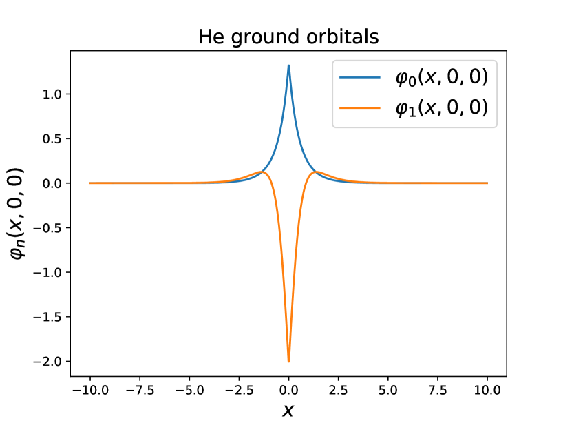
Figure 1. Two determinants ground state of the helium atom with the coefficients $c_{0}=0.99793$ and $c_{1}=-0.06430$, correspondingly. The corresponding total energy is $-2.87799$.

5. Symmetric hessian and shift

In the previous section we did not bother to define $\mathcal{R}(w)$ so the operator $d\mathcal{R}(w)$ is symmetric. However, the hermitian property of the second derivative is important for introducing the Levenberg–Marquardt damping $\lambda\geqslant 0$. The Lagrangian is defined by

$$\mathcal{L}=\frac{1}{4}E-\frac{1}{2}\sum_{i,j=1}^{2}\varepsilon_{ij}\left(\int\varphi_{i}\varphi_{j}-\delta_{ij}\right)$$

with symmetric matrix $\varepsilon$ and variational derivatives

$$\frac{\delta\mathcal{L}}{\delta\varphi_{1}}=c_{1}^{2}\left(h+\frac{1}{|x|}*\varphi_{1}^{2}\right)\varphi_{1}+c_{1}c_{2}\left(\frac{1}{|x|}*(\varphi_{1}\varphi_{2})\right)\varphi_{2}-\varepsilon_{11}\varphi_{1}-\varepsilon_{12}\varphi_{2}$$ (5.1)

$$\frac{\delta\mathcal{L}}{\delta\varphi_{2}}=c_{2}^{2}\left(h+\frac{1}{|x|}*\varphi_{2}^{2}\right)\varphi_{2}+c_{1}c_{2}\left(\frac{1}{|x|}*(\varphi_{1}\varphi_{2})\right)\varphi_{1}-\varepsilon_{12}\varphi_{1}-\varepsilon_{22}\varphi_{2}$$

where $c_{1}=\cos\theta$ and $c_{2}=\sin\theta$. The derivatives with respect to scalars are

$$\frac{\partial\mathcal{L}}{\partial\theta}=-\frac{1}{4}\sin 2\theta(2(1|h|1)+(11|11))+\frac{1}{4}\sin 2\theta(2(2|h|2)+(22|22))+\frac{1}{2}\cos 2\theta(12|12)$$

and

$$\frac{\partial\mathcal{L}}{\partial\varepsilon_{11}} =-\frac{1}{2}\left(\left\|\varphi_{1}\right\|^{2}-1\right)$$ (5.2)

$$\frac{\partial\mathcal{L}}{\partial\varepsilon_{22}} =-\frac{1}{2}\left(\left\|\varphi_{2}\right\|^{2}-1\right)$$

$$\frac{\partial\mathcal{L}}{\partial\varepsilon_{12}} =-\int\varphi_{1}\varphi_{2}$$

We introduce

$$\mathcal{R}(\varphi_{1},\varphi_{2},\theta,\varepsilon_{11},\varepsilon_{22},\varepsilon_{12})=\nabla\mathcal{L}=\left(\frac{\delta\mathcal{L}}{\delta\varphi_{1}},\frac{\delta\mathcal{L}}{\delta\varphi_{2}},\frac{\partial\mathcal{L}}{\partial\theta},\frac{\partial\mathcal{L}}{\partial\varepsilon_{11}},\frac{\partial\mathcal{L}}{\partial\varepsilon_{22}},\frac{\partial\mathcal{L}}{\partial\varepsilon_{12}}\right)^{T}$$

acting in $W=L^{2}\left(\mathbb{R}^{3}\right)^{2}\times\mathbb{R}^{4}.$ Now for a given $w=w_{n}\in W$ we solve the shifted Newton’s equation

$$(d\mathcal{R}(w)+\lambda)\delta w=-\mathcal{R}(w),\quad\lambda\geqslant 0,$$

with respect $\delta w\in W$. This is a linear equation that we solve iteratively and accelerating with DIIS. The Jacobian $d\mathcal{R}(w)$ equals to the Hessian $d\nabla\mathcal{L}(w)$. Then the update is $w_{n+1}=w_{n}+\delta w$.

$$d\mathcal{R}_{i}(w)\delta w=\partial_{\varphi_{1}}\mathcal{R}_{i}(w)\delta\varphi_{1}+\ldots+\frac{\partial\mathcal{R}_{i}}{\partial\varepsilon_{12}}(w)\delta\varepsilon_{12},\quad i=1,2,$$

where the first partial derivative is applied to $\delta\varphi_{1}$ as a linear operator in $L^{2}$, and the last partial derivative is a function multiplied by the scalar $\delta\varepsilon_{12}$. The differential of first component $d\mathcal{R}_{1}(w)\delta w$ consists of

$$\partial_{\varphi_{1}}\mathcal{R}_{1}(w)\delta\varphi_{1}=c_{1}^{2}\left(h+\frac{1}{|x|}*\varphi_{1}^{2}\right)\delta\varphi_{1}+2c_{1}^{2}\left(\frac{1}{|x|}*(\delta\varphi_{1}\varphi_{1})\right)\varphi_{1}+c_{1}c_{2}\left(\frac{1}{|x|}*(\delta\varphi_{1}\varphi_{2})\right)\varphi_{2}-\varepsilon_{11}\delta\varphi_{1},$$

$$\partial_{\varphi_{2}}\mathcal{R}_{1}(w)\delta\varphi_{2}=c_{1}c_{2}\left(\frac{1}{|x|}*(\varphi_{1}\delta\varphi_{2})\right)\varphi_{2}+c_{1}c_{2}\left(\frac{1}{|x|}*(\varphi_{1}\varphi_{2})\right)\delta\varphi_{2}-\varepsilon_{12}\delta\varphi_{2},$$

$$\frac{\partial\mathcal{R}_{1}}{\partial\theta}(w)\delta\theta=-\delta\theta\sin 2\theta\left(h+\frac{1}{|x|}*\varphi_{1}^{2}\right)\varphi_{1}+\delta\theta\cos 2\theta\left(\frac{1}{|x|}*(\varphi_{1}\varphi_{2})\right)\varphi_{2}$$

and the rest

$$\frac{\partial\mathcal{R}_{1}}{\partial\varepsilon_{11}}(w)\delta\varepsilon_{11}+\frac{\partial\mathcal{R}_{1}}{\partial\varepsilon_{22}}(w)\delta\varepsilon_{22}+\frac{\partial\mathcal{R}_{1}}{\partial\varepsilon_{12}}(w)\delta\varepsilon_{12}=-\delta\varepsilon_{11}\varphi_{1}-\delta\varepsilon_{12}\varphi_{2}$$

Similarly, $d\mathcal{R}_{2}(w)\delta w$ consists of

$$\partial_{\varphi_{1}}\mathcal{R}_{2}(w)\delta\varphi_{1}=c_{1}c_{2}\left(\frac{1}{|x|}*(\delta\varphi_{1}\varphi_{2})\right)\varphi_{1}+c_{1}c_{2}\left(\frac{1}{|x|}*(\varphi_{1}\varphi_{2})\right)\delta\varphi_{1}-\varepsilon_{12}\delta\varphi_{1},$$

$$\partial_{\varphi_{2}}\mathcal{R}_{2}(w)\delta\varphi_{2}=c_{2}^{2}\left(h+\frac{1}{|x|}*\varphi_{2}^{2}\right)\delta\varphi_{2}+2c_{2}^{2}\left(\frac{1}{|x|}*(\delta\varphi_{2}\varphi_{2})\right)\varphi_{2}+c_{1}c_{2}\left(\frac{1}{|x|}*(\varphi_{1}\delta\varphi_{2})\right)\varphi_{1}-\varepsilon_{22}\delta\varphi_{2},$$

$$\frac{\partial\mathcal{R}_{2}}{\partial\theta}(w)\delta\theta=\delta\theta\sin 2\theta\left(h+\frac{1}{|x|}*\varphi_{2}^{2}\right)\varphi_{2}+\delta\theta\cos 2\theta\left(\frac{1}{|x|}*(\varphi_{1}\varphi_{2})\right)\varphi_{1}$$

and the remaining terms

$$\frac{\partial\mathcal{R}_{2}}{\partial\varepsilon_{11}}(w)\delta\varepsilon_{11}+\frac{\partial\mathcal{R}_{2}}{\partial\varepsilon_{22}}(w)\delta\varepsilon_{22}+\frac{\partial\mathcal{R}_{2}}{\partial\varepsilon_{12}}(w)\delta\varepsilon_{12}=-\delta\varepsilon_{12}\varphi_{1}-\delta\varepsilon_{22}\varphi_{2}$$

The differential of third component $d\mathcal{R}_{3}(w)\delta w$ consists of

$$\partial_{\varphi_{1}}\mathcal{R}_{3}(w)\delta\varphi_{1}=-\sin 2\theta((\delta 1|h|1)+(\delta 11|11))+\cos 2\theta(\delta 12|12)$$

$$\partial_{\varphi_{2}}\mathcal{R}_{3}(w)\delta\varphi_{2}=\sin 2\theta((\delta 2|h|2)+(\delta 22|22))+\cos 2\theta(1\delta 2|12)$$

$$\frac{\partial\mathcal{R}_{3}}{\partial\theta}(w)\delta\theta=\left(-\frac{1}{2}\cos 2\theta(2(1|h|1)+(11|11))+\frac{1}{2}\cos 2\theta(2(2|h|2)+(22|22))-\sin 2\theta(12|12)\right)\delta\theta$$

Finally,

$$d\mathcal{R}_{4}(w)\delta w=\partial_{\varphi_{1}}\mathcal{R}_{4}(w)\delta\varphi_{1}=-\int\varphi_{1}\delta\varphi_{1}$$

$$d\mathcal{R}_{5}(w)\delta w=\partial_{\varphi_{2}}\mathcal{R}_{5}(w)\delta\varphi_{2}=-\int\varphi_{2}\delta\varphi_{2}$$

$$d\mathcal{R}_{6}(w)\delta w=\partial_{\varphi_{1}}\mathcal{R}_{6}(w)\delta\varphi_{1}+\partial_{\varphi_{2}}\mathcal{R}_{6}(w)\delta\varphi_{2}=-\int\delta\varphi_{1}\varphi_{2}-\int\varphi_{1}\delta\varphi_{2}$$

This finishes the detailed description of the Newton equation. Now we want to rewrite it in the self-consistent form, which will be suitable for an iterative procedure.

5.1. Self-consistent form

We rewrite the Newton equation in the form

$$(\delta\varphi_{1},\delta\varphi_{2})^{T}=\mathbb{F}(\delta\varphi_{1},\delta\varphi_{2};w),$$

where $w=(\varphi_{1},\varphi_{2},\theta,\varepsilon_{11},\varepsilon_{22},\varepsilon_{12})$ is fixed at each Newton step, as follows. Firstly, $\delta\theta$ is defined as $\delta\theta=\Theta(\delta\varphi_{1},\delta\varphi_{2},w)$ by

$$\delta\theta=-\left(\frac{\partial\mathcal{R}_{3}}{\partial\theta}(w)+\lambda\right)^{-1}\left(\partial_{\varphi_{1}}\mathcal{R}_{3}(w)\delta\varphi_{1}+\partial_{\varphi_{2}}\mathcal{R}_{3}(w)\delta\varphi_{2}+\mathcal{R}_{3}(w)\right)$$

Secondly, $\delta\varepsilon_{ij}$ are defined by $\delta\varepsilon_{ij}=\mathcal{E}_{ij}(\delta\varphi_{1},\delta\varphi_{2},\delta\theta,w)$ that we introduce as follows. We rewrite the first two lines of the Newton’s system as

$$\delta\varepsilon_{11}\varphi_{1}+\delta\varepsilon_{12}\varphi_{2}+(\varepsilon_{11}-\lambda)\delta\varphi_{1}+\varepsilon_{12}\delta\varphi_{2}=F(\delta\varphi_{1},\delta\varphi_{2},\delta\theta,w)$$ (5.3)

$$\delta\varepsilon_{12}\varphi_{1}+\delta\varepsilon_{22}\varphi_{2}+\varepsilon_{12}\delta\varphi_{1}+(\varepsilon_{22}-\lambda)\delta\varphi_{2}=G(\delta\varphi_{1},\delta\varphi_{2},\delta\theta,w)$$

Multiplying these equations by $\varphi_{1}$, $\varphi_{2}$ and then integrating, we obtain four equations in $\mathbb{R}$. We exclude $\int\varphi_{1}\delta\varphi_{1}$ and $\int\varphi_{2}\delta\varphi_{2}$ using the fourth and the fifth Newton equations. Finally, complementing these four equations by the sixth Newton equation we obtain the following system

$$\begin{pmatrix}\left\|\varphi_{1}\right\|^{2}+(\varepsilon_{11}-\lambda)\lambda&0&\int\varphi_{1}\varphi_{2}&0&\varepsilon_{12}\\ 0&\left\|\varphi_{2}\right\|^{2}+(\varepsilon_{22}-\lambda)\lambda&\int\varphi_{1}\varphi_{2}&\varepsilon_{12}&0\\ \int\varphi_{1}\varphi_{2}&0&\left\|\varphi_{2}\right\|^{2}&\varepsilon_{11}-\lambda&0\\ 0&\int\varphi_{1}\varphi_{2}&\left\|\varphi_{1}\right\|^{2}&0&\varepsilon_{22}-\lambda\\ 0&0&-\lambda&1&1\end{pmatrix}\begin{pmatrix}\delta\varepsilon_{11}\\ \delta\varepsilon_{22}\\ \delta\varepsilon_{12}\\ \int\delta\varphi_{1}\varphi_{2}\\ \int\varphi_{1}\delta\varphi_{2}\end{pmatrix}\\ =\begin{pmatrix}\int F\varphi_{1}-\frac{1}{2}(\varepsilon_{11}-\lambda)\left(1-\left\|\varphi_{1}\right\|^{2}\right)\\ \int G\varphi_{2}-\frac{1}{2}(\varepsilon_{22}-\lambda)\left(1-\left\|\varphi_{2}\right\|^{2}\right)\\ \int F\varphi_{2}-\frac{1}{2}\varepsilon_{12}\left(1-\left\|\varphi_{2}\right\|^{2}\right)\\ \int G\varphi_{1}-\frac{1}{2}\varepsilon_{12}\left(1-\left\|\varphi_{1}\right\|^{2}\right)\\ -\int\varphi_{1}\varphi_{2}\end{pmatrix}$$ (5.4)

We search for orthonormal orbitals $\varphi_{1},\varphi_{2}$. Therefore, the determinant of this system should stay close to $-\varepsilon_{11}-\varepsilon_{22}$ during each Newton’s update, provided $\lambda=0$. In particular, the matrix should be invertible for each Newton’s iteration $w=w_{n}$.

$$\int F\varphi_{1}=c_{1}^{2}(\delta 1|h|1)+3c_{1}^{2}(\delta 11|11)+c_{1}c_{2}(\delta 12|12)+2c_{1}c_{2}(1\delta 2|12)\\ +(c_{1}^{2}-\delta\theta\sin 2\theta)((1|h|1)+(11|11))+(c_{1}c_{2}+\delta\theta\cos 2\theta)(12|12)-\varepsilon_{11}\left\|\varphi_{1}\right\|^{2}-\varepsilon_{12}\int\varphi_{1}\varphi_{2}$$ (5.5)

$$\int F\varphi_{2}=c_{1}^{2}(\delta 1|h|2)+c_{1}^{2}(\delta 12|11)+2c_{1}^{2}(\delta 11|12)+c_{1}c_{2}(\delta 12|22)+c_{1}c_{2}(1\delta 2|22)+c_{1}c_{2}(2\delta 2|12)\\ +(c_{1}^{2}-\delta\theta\sin 2\theta)((1|h|2)+(11|12))+(c_{1}c_{2}+\delta\theta\cos 2\theta)(12|22)-\varepsilon_{11}\int\varphi_{1}\varphi_{2}-\varepsilon_{12}\left\|\varphi_{2}\right\|^{2}$$ (5.6)

$$\int G\varphi_{2}=c_{2}^{2}(\delta 2|h|2)+3c_{2}^{2}(\delta 22|22)+2c_{1}c_{2}(\delta 12|12)+c_{1}c_{2}(1\delta 2|12)\\ +(c_{2}^{2}+\delta\theta\sin 2\theta)((2|h|2)+(22|22))+(c_{1}c_{2}+\delta\theta\cos 2\theta)(12|12)-\varepsilon_{22}\left\|\varphi_{2}\right\|^{2}-\varepsilon_{12}\int\varphi_{1}\varphi_{2}$$ (5.7)

$$\int G\varphi_{1}=c_{2}^{2}(\delta 2|h|1)+c_{2}^{2}(1\delta 2|22)+2c_{2}^{2}(\delta 22|12)+c_{1}c_{2}(\delta 12|11)+c_{1}c_{2}(1\delta 2|11)+c_{1}c_{2}(1\delta 1|12)\\ +(c_{2}^{2}+\delta\theta\sin 2\theta)((1|h|2)+(12|22))+(c_{1}c_{2}+\delta\theta\cos 2\theta)(11|12)-\varepsilon_{22}\int\varphi_{1}\varphi_{2}-\varepsilon_{12}\left\|\varphi_{1}\right\|^{2}$$ (5.8)

It is left to rewrite the $L^{2}$-equations as

$$\left(-\frac{c_{1}^{2}}{2}\Delta-\varepsilon_{11}+\lambda\right)\delta\varphi_{1}+\left(1-\frac{\delta\theta\sin 2\theta}{c_{1}^{2}}\right)\left(-\frac{c_{1}^{2}}{2}\Delta-\varepsilon_{11}+\lambda\right)\varphi_{1}\\ +c_{1}^{2}\left(V_{\text{nuc}}+J(11)\right)\delta\varphi_{1}+2c_{1}^{2}J(1\delta 1)\varphi_{1}+c_{1}c_{2}J(\delta 12)\varphi_{2}+c_{1}c_{2}J(1\delta 2)\varphi_{2}+c_{1}c_{2}J(12)\delta\varphi_{2}-\varepsilon_{12}\delta\varphi_{2}\\ -\delta\varepsilon_{12}\varphi_{2}-\varepsilon_{12}\varphi_{2}-\left((\varepsilon_{11}-\lambda)\frac{\delta\theta\sin 2\theta}{c_{1}^{2}}+\delta\varepsilon_{11}+\lambda\right)\varphi_{1}\\ +\left(c_{1}^{2}-\delta\theta\sin 2\theta\right)\left(V_{\text{nuc}}+J(11)\right)\varphi_{1}+(c_{1}c_{2}+\delta\theta\cos 2\theta)J(12)\varphi_{2}=0$$ (5.9)

$$\left(-\frac{c_{2}^{2}}{2}\Delta-\varepsilon_{22}+\lambda\right)\delta\varphi_{2}+\left(1+\frac{\delta\theta\sin 2\theta}{c_{2}^{2}}\right)\left(-\frac{c_{2}^{2}}{2}\Delta-\varepsilon_{22}+\lambda\right)\varphi_{2}\\ +c_{1}c_{2}J(\delta 12)\varphi_{1}+c_{1}c_{2}J(12)\delta\varphi_{1}+2c_{2}^{2}J(2\delta 2)\varphi_{2}+c_{1}c_{2}J(1\delta 2)\varphi_{1}-\varepsilon_{12}\delta\varphi_{1}+c_{2}^{2}\left(V_{\text{nuc}}+J(22)\right)\delta\varphi_{2}\\ -\delta\varepsilon_{12}\varphi_{1}-\varepsilon_{12}\varphi_{1}+\left((\varepsilon_{22}-\lambda)\frac{\delta\theta\sin 2\theta}{c_{2}^{2}}-\delta\varepsilon_{22}-\lambda\right)\varphi_{2}\\ +\left(c_{2}^{2}+\delta\theta\sin 2\theta\right)\left(V_{\text{nuc}}+J(22)\right)\varphi_{2}+(c_{1}c_{2}+\delta\theta\cos 2\theta)J(12)\varphi_{1}=0$$ (5.10)

Finally, introducing

$$R_{i}^{\lambda}=\left(-\frac{c_{i}^{2}}{2}\Delta-\varepsilon_{ii}+\lambda\right)^{-1}=\frac{2}{c_{i}^{2}}H\left(\sqrt{\frac{2(\lambda-\varepsilon_{ii})}{c_{i}^{2}}}\right)=\frac{2}{c_{i}^{2}}H\left(\mu_{i}\right)=\frac{2}{c_{i}^{2}}\left(-\Delta+\mu_{i}^{2}\right)^{-1}$$

$$\delta\varphi_{1}=-\left(1-\frac{\delta\theta\sin 2\theta}{c_{1}^{2}}\right)\varphi_{1}-R_{1}^{\lambda}\mathfrak{F}_{1}^{\lambda}$$ (5.11)

$$\delta\varphi_{2}=-\left(1+\frac{\delta\theta\sin 2\theta}{c_{2}^{2}}\right)\varphi_{2}-R_{2}^{\lambda}\mathfrak{F}_{2}^{\lambda}$$

$$\mathfrak{F}_{1}^{\lambda}=-\varepsilon_{12}\delta\varphi_{2}-(\delta\varepsilon_{12}+\varepsilon_{12})\varphi_{2}-\left((\varepsilon_{11}-\lambda)\frac{\delta\theta\sin 2\theta}{c_{1}^{2}}+\delta\varepsilon_{11}+\lambda\right)\varphi_{1}\\ +\left(V_{\text{nuc}}+J(11)\right)\left(c_{1}^{2}\delta\varphi_{1}+\left(c_{1}^{2}-\delta\theta\sin 2\theta\right)\varphi_{1}\right)+J(12)(c_{1}c_{2}\delta\varphi_{2}+(c_{1}c_{2}+\delta\theta\cos 2\theta)\varphi_{2})\\ +2c_{1}^{2}J(1\delta 1)\varphi_{1}+c_{1}c_{2}J(\delta 12)\varphi_{2}+c_{1}c_{2}J(1\delta 2)\varphi_{2}$$

$$\mathfrak{F}_{2}^{\lambda}=-\varepsilon_{12}\delta\varphi_{1}-(\delta\varepsilon_{12}+\varepsilon_{12})\varphi_{1}+\left((\varepsilon_{22}-\lambda)\frac{\delta\theta\sin 2\theta}{c_{2}^{2}}-\delta\varepsilon_{22}-\lambda\right)\varphi_{2}\\ +\left(V_{\text{nuc}}+J(22)\right)\left(c_{2}^{2}\delta\varphi_{2}+\left(c_{2}^{2}+\delta\theta\sin 2\theta\right)\varphi_{2}\right)+J(12)(c_{1}c_{2}\delta\varphi_{1}+(c_{1}c_{2}+\delta\theta\cos 2\theta)\varphi_{1})\\ +2c_{2}^{2}J(2\delta 2)\varphi_{2}+c_{1}c_{2}J(\delta 12)\varphi_{1}+c_{1}c_{2}J(1\delta 2)\varphi_{1}$$

For $\lambda=0$ the final Newton system obviously coincides with the system derived in the previous section. The importance of defining the Newton’s function consistently, namely, as $\mathcal{R}=\nabla\mathcal{L}$, is obvious, provided one uses the Levenberg–Marquardt damping $\lambda\geqslant 0$ or any other special technique tailored for Newton’s optimization. It is worth to point out, that as long as $\lambda$ is small, $\left(V_{\text{nuc}}+J(ii)-\lambda\right)\varphi_{i}\approx\left(V_{\text{nuc}}+J(ii)\right)\varphi_{i}.$ Therefore, the damping affects directly only the diagonal orbital energies $\varepsilon_{ii}$. In fact, one can use a different $\lambda_{i}$ for every energy $\varepsilon_{ii}$. This justifies the trick of controlling and correcting the sign of $\varepsilon_{ii}$ during numerical simulations, from the abstract optimization perspective. Keeping this in mind below, we omit the use of the damping in the formulas. In actual simulations we modify energies diagonal orbital energies $\varepsilon_{ii}$, as long as we encounter a positive value or if Newton’s step fails providing a lower energy value.

6. General case

The wave function is represented as a sum of $M+1$ closed shell determinants

$$\Psi=\sum_{m=0}^{M}c_{m}\left|m\overline{m}\right\rangle$$

Then the total energy takes the quadratic form

$$E=\left\langle\Psi\left|\widehat{H}\right|\Psi\right\rangle=\sum_{k,m=0}^{M}H_{km}c_{k}c_{m},$$

where the energy matrix elements are

$$H_{km}=\left\langle k\overline{k}\left|\widehat{H}\right|m\overline{m}\right\rangle=2\delta_{km}(k|h|m)+(km|km)$$

Introduce the Lagrangian

$$\mathcal{L}=\frac{1}{4}E-\frac{1}{4}\varepsilon\left(\sum_{m=0}^{M}c_{m}^{2}-1\right)-\frac{1}{2}\sum_{i,j=0}^{M}\varepsilon_{ij}\left(\int\varphi_{i}\varphi_{j}-\delta_{ij}\right)$$

with symmetric matrix coefficients $\varepsilon_{ij}$. It is a function of $\varphi_{0},\ldots,\varphi_{M},\varepsilon,c_{0},\ldots,c_{M}$ and $\varepsilon_{ij}$ with $i\leqslant j$. We calculate its gradient as follows. Firstly, the variational derivatives

$$\frac{\delta\mathcal{L}}{\delta\varphi_{k}} =c_{k}^{2}h\varphi_{k}+c_{k}\sum_{m=0}^{M}c_{m}J(km)\varphi_{m}-\sum_{m=0}^{M}\varepsilon_{km}\varphi_{m},\quad k=0,\ldots,M.$$ (6.1)

$$\frac{\partial\mathcal{L}}{\partial\varepsilon} =-\frac{1}{4}\left(\sum_{m=0}^{M}c_{m}^{2}-1\right).$$ (6.2)

$$\frac{\partial\mathcal{L}}{\partial c_{k}} =\frac{1}{2}\sum_{m=0}^{M}H_{km}c_{m}-\frac{1}{2}\varepsilon c_{k},\quad k=0,\ldots,M.$$ (6.3)

$$\frac{\partial\mathcal{L}}{\partial\varepsilon_{kk}} =-\frac{1}{2}\left(\left\|\varphi_{k}\right\|^{2}-1\right),\quad k=0,\ldots,M,$$ (6.4)

$$\frac{\partial\mathcal{L}}{\partial\varepsilon_{ij}} =-\int\varphi_{i}\varphi_{j},\quad 0\leqslant i<j\leqslant M.$$ (6.5)

Now let us calculate the Hessian $d\nabla\mathcal{L}$.

$$\sum_{j=0}^{M}\partial_{\varphi_{j}}\frac{\delta\mathcal{L}}{\delta\varphi_{k}}\delta\varphi_{j}=c_{k}^{2}h\delta\varphi_{k}-\sum_{m=0}^{M}\varepsilon_{km}\delta\varphi_{m}+c_{k}\sum_{m=0}^{M}c_{m}\left(J(\delta km)\varphi_{m}+J(k\delta m)\varphi_{m}+J(km)\delta\varphi_{m}\right),$$ (6.6)

where $k=0,\ldots,M.$

$$\frac{\partial}{\partial\varepsilon}\frac{\delta\mathcal{L}}{\delta\varphi_{k}}=0$$

$$\sum_{j=0}^{M}\frac{\partial}{\partial c_{j}}\frac{\delta\mathcal{L}}{\delta\varphi_{k}}\delta c_{j}=2c_{k}\delta c_{k}h\varphi_{k}+\delta c_{k}\sum_{m=0}^{M}c_{m}J(km)\varphi_{m}+c_{k}\sum_{m=0}^{M}\delta c_{m}J(km)\varphi_{m}$$

$$\sum_{0\leqslant i\leqslant j\leqslant M}\frac{\partial}{\partial\varepsilon_{ij}}\frac{\delta\mathcal{L}}{\delta\varphi_{k}}\delta\varepsilon_{ij}=-\sum_{m=0}^{M}\delta\varepsilon_{km}\varphi_{m},$$

where we extended the orbital energy update by symmetry. Summing these equalities we obtain

$$d\frac{\delta\mathcal{L}}{\delta\varphi_{k}}\delta w=c_{k}^{2}h\delta\varphi_{k}-\sum_{m=0}^{M}\varepsilon_{km}\delta\varphi_{m}+c_{k}\sum_{m=0}^{M}c_{m}\left(J(\delta km)\varphi_{m}+J(k\delta m)\varphi_{m}+J(km)\delta\varphi_{m}\right)\\ +2c_{k}\delta c_{k}h\varphi_{k}+\delta c_{k}\sum_{m=0}^{M}c_{m}J(km)\varphi_{m}+c_{k}\sum_{m=0}^{M}\delta c_{m}J(km)\varphi_{m}-\sum_{m=0}^{M}\delta\varepsilon_{km}\varphi_{m}$$ (6.6)

$$d\frac{\partial\mathcal{L}}{\partial\varepsilon}\delta w=-\frac{1}{2}\sum_{m=0}^{M}c_{m}\delta c_{m}$$ (LHS2)

$$\sum_{j=0}^{M}\partial_{\varphi_{j}}\frac{\partial\mathcal{L}}{\partial c_{k}}\delta\varphi_{j}=2c_{k}(\delta k|h|k)+\sum_{m=0}^{M}c_{m}(\delta km|km)+\sum_{m=0}^{M}c_{m}(k\delta m|km)$$

$$\frac{\partial}{\partial{\varepsilon}}\frac{\partial\mathcal{L}}{\partial c_{k}}\delta\varepsilon=-\frac{1}{2}\delta\varepsilon c_{k}$$

$$\sum_{j=0}^{M}\frac{\partial}{\partial c_{j}}\frac{\partial\mathcal{L}}{\partial c_{k}}\delta c_{j}=\frac{1}{2}\sum_{m=0}^{M}H_{km}\delta c_{m}-\frac{1}{2}\varepsilon\delta c_{k}$$

Summing these equalities we obtain

$$d\frac{\partial\mathcal{L}}{\partial c_{k}}\delta w=2c_{k}(\delta k|h|k)+\sum_{m=0}^{M}c_{m}(\delta km|km)+\sum_{m=0}^{M}c_{m}(k\delta m|km)-\frac{1}{2}\delta\varepsilon c_{k}+\frac{1}{2}\sum_{m=0}^{M}H_{km}\delta c_{m}-\frac{1}{2}\varepsilon\delta c_{k}$$ (LHS3)

Finally,

$$d\frac{\partial\mathcal{L}}{\partial\varepsilon_{kk}}\delta w=-\int\varphi_{k}\delta\varphi_{k},\quad k=0,\ldots,M,$$ (LHS4)

$$d\frac{\partial\mathcal{L}}{\partial\varepsilon_{ij}}\delta w=-\int\delta\varphi_{i}\varphi_{j}-\int\varphi_{i}\delta\varphi_{j},\quad 0\leqslant i<j\leqslant M.$$ (LHS5)

The right hand side is $-\nabla\mathcal{L}$. This finishes the detailed description of the Newton equation. Now we want to rewrite it in the self-consistent form, which will be suitable for an iterative procedure.

6.1. Self-consistent form

We rewrite the Newton equation in the form

$$\delta\varphi_{k}=\mathbb{F}_{k}(\delta\varphi_{0},\ldots,\delta\varphi_{M};w),\quad k=0,\ldots,M,$$ (6.7)

where $w=(\varphi_{1},\ldots,\varepsilon_{M-1,M})$ is fixed at each Newton step, as follows.

$$\begin{pmatrix}0&c_{0}&\cdots&c_{M}\\ c_{0}&&&\\ \vdots&&\varepsilon-H&\\ c_{M}&&&\end{pmatrix}\begin{pmatrix}\delta\varepsilon\\ \delta c_{0}\\ \vdots\\ \delta c_{M}\end{pmatrix}=\begin{pmatrix}-\frac{1}{2}\left(\sum_{m=0}^{M}c_{m}^{2}-1\right)\\ f\end{pmatrix}$$

$$\begin{pmatrix}0&\mathbf{c}^{T}\\ \mathbf{c}&\varepsilon-H\end{pmatrix}\begin{pmatrix}\delta\varepsilon\\ \delta\mathbf{c}\end{pmatrix}=\begin{pmatrix}-\frac{1}{2}\left(\sum_{m=0}^{M}c_{m}^{2}-1\right)\\ f\end{pmatrix}$$

where: $\mathbf{c}=(c_{0},c_{1},\dots,c_{M})^{T}$ is a column vector, $\varepsilon-H$ is an $(M+1)\times(M+1)$ matrix. Here

$$f_{k}=\sum_{m=0}^{M}H_{km}c_{m}-\varepsilon c_{k}+4c_{k}(\delta k|h|k)+2\sum_{m=0}^{M}c_{m}(\delta km|km)+2\sum_{m=0}^{M}c_{m}(k\delta m|km),\quad k=0,\ldots,M$$

Introduce the matrix

$$F_{kj}=\int\left(d\frac{\delta\mathcal{L}}{\delta\varphi_{k}}\delta w+\frac{\delta\mathcal{L}}{\delta\varphi_{k}}+\sum_{m=0}^{M}\delta\varepsilon_{km}\varphi_{m}+\sum_{m=0}^{M}\varepsilon_{km}\delta\varphi_{m}\right)\varphi_{j}=c_{k}^{2}(\delta k|h|j)\\ +c_{k}\sum_{m=0}^{M}c_{m}\left((\delta km|jm)+(k\delta m|jm)+(j\delta m|km)\right)+2c_{k}\delta c_{k}(k|h|j)+\sum_{m=0}^{M}(c_{k}\delta c_{m}+\delta c_{k}c_{m})(jm|km)\\ +c_{k}^{2}(k|h|j)+c_{k}\sum_{m=0}^{M}c_{m}(jm|km)-\underbrace{\sum_{m=0}^{M}\varepsilon_{km}\int\varphi_{j}\varphi_{m}}_{=\varepsilon_{jk}}$$

So far the derivation of the self-consistent form was generic. In order to simplify the equations we will assume from now on, that the orbitals are normalized as $\int\varphi_{j}\varphi_{m}=\delta_{jm}.$ Note that this normalization is needed to accelerate the Newton optimization, as we have seen above. This also simplifies the equations for the orbital energy updates $\delta\varepsilon_{kj}$ into the following matrix form

$$X+\mathcal{E}Y=F,$$

where $\mathcal{E}=(\varepsilon_{kj})$, $X=(\delta\varepsilon_{kj})$ is symmetric and $Y=\left(\int\delta\varphi_{j}\varphi_{k}\right)$ is antisymmetric. As long as the spectra of $\mathcal{E}$ and $-\mathcal{E}$ are disjoint, there exist a unique solution $X$. For this it is enough to have all the eigenvalues of $\mathcal{E}$ being negative. One naturally anticipates the orbital energies to be negative. Taking the transpose of both sides and accounting for $X^{T}=X$, $Y^{T}=-Y$ one obtains

$$X-Y\mathcal{E}^{T}=F^{T}.$$

Now, we add and subtract the original equation in order to simplify to two separate equations:

$$2X=(F+F^{T})-\mathcal{E}Y+Y\mathcal{E}^{T},$$

$$\mathcal{E}Y+Y\mathcal{E}^{T}=(F-F^{T}).$$

The equation for $Y$ is a Sylvester equation, which can be solved by the Bartels–Stewart algorithm implemented in many software packages. Its computational cost is $\mathcal{O}\left(M^{3}\right)$ arithmetical operations, that can be viewed negligible. Once $Y$ is found, we solve for $X$:

$$X=\frac{1}{2}(F+F^{T}+\mathcal{E}Y^{T}+Y\mathcal{E}^{T}).$$

This ensures that $X=(\delta\varepsilon_{kj})$ remains symmetric. The second matrix $Y$ is not needed by itself.

It is left to precondition the first $M+1$ equations in the Newton system

$$d\frac{\delta\mathcal{L}}{\delta\varphi_{k}}\delta w+\frac{\delta\mathcal{L}}{\delta\varphi_{k}}=0$$

as follows

$$\left(-\frac{c_{k}^{2}}{2}\Delta-\varepsilon_{kk}\right)\delta\varphi_{k}+\left(1+\frac{2\delta c_{k}}{c_{k}}\right)\left(-\frac{c_{k}^{2}}{2}\Delta-\varepsilon_{kk}\right)\varphi_{k}+\left(\frac{2\delta c_{k}}{c_{k}}\varepsilon_{kk}-\delta\varepsilon_{kk}\right)\varphi_{k}\\ +c_{k}^{2}V_{\text{nuc}}\left(\left(1+\frac{2\delta c_{k}}{c_{k}}\right)\varphi_{k}+\delta\varphi_{k}\right)-\sum_{\begin{subarray}{c}m=0\\ m\neq k\end{subarray}}^{M}\left(\varepsilon_{km}\delta\varphi_{m}+\delta\varepsilon_{km}\varphi_{m}+\varepsilon_{km}\varphi_{m}\right)\\ +\delta c_{k}\sum_{m=0}^{M}c_{m}J(km)\varphi_{m}+c_{k}\sum_{m=0}^{M}\delta c_{m}J(km)\varphi_{m}+c_{k}\sum_{m=0}^{M}c_{m}J(km)(\varphi_{m}+\delta\varphi_{m})\\ +c_{k}\sum_{m=0}^{M}c_{m}\left(J(\delta km)\varphi_{m}+J(k\delta m)\varphi_{m}\right)=0$$

Finally,

$$\delta\varphi_{k}=-\left(1+\frac{2\delta c_{k}}{c_{k}}\right)\varphi_{k}-R_{k}\mathfrak{F}_{k}$$ (6.8)

where

$$\mathfrak{F}_{k}=\left(\frac{2\delta c_{k}}{c_{k}}\varepsilon_{kk}-\delta\varepsilon_{kk}\right)\varphi_{k}+c_{k}^{2}V_{\text{nuc}}\left(\left(1+\frac{2\delta c_{k}}{c_{k}}\right)\varphi_{k}+\delta\varphi_{k}\right)\\ -\sum_{\begin{subarray}{c}m=0\\ m\neq k\end{subarray}}^{M}\left(\varepsilon_{km}\delta\varphi_{m}+\delta\varepsilon_{km}\varphi_{m}+\varepsilon_{km}\varphi_{m}\right)+\sum_{m=0}^{M}J(km)\left((\delta c_{k}c_{m}+c_{k}\delta c_{m}+c_{k}c_{m})\varphi_{m}+c_{k}c_{m}\delta\varphi_{m}\right)\\ +c_{k}\sum_{m=0}^{M}c_{m}\left(J(\delta km)\varphi_{m}+J(k\delta m)\varphi_{m}\right)$$

and the convolution operator $R_{k}$ is defined as above. This finishes the description of $\mathbb{F}_{k}$ in (6.7).

6.2. Numerics

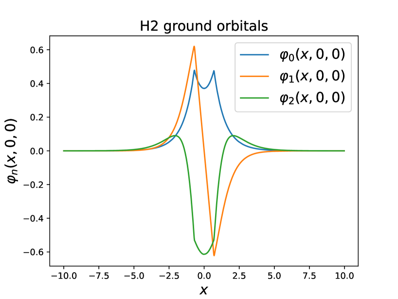
Figure 2. Three determinants ground state of the hydrogen molecule with the coefficients $c_{0}=0.99253,c_{1}=-0.10718$ and $c_{2}=-0.05829$, accordingly. The corresponding energy is $-1.15949$.

The default calculation settings: maximum 15 iterations for the inner loop related to the treatment of each Newton’s equation. We use DIIS with maximum 3 previous iterations. The initial trust radius is set to 1.0 and modified by dividing in two every time the new iteration results in a bigger energy value. In addition, we modify the diagonal values of the orbital energies by multiplying by 10. We initialize the orbital energy matrix by $\mathds{1}$ at the beginning. One may reset the orbital energy matrix back to $-\mathds{1}$ at the end of the first few iterations, in order to avoid unwanted saddle points.

Figure 3. Newton energy optimization step.

After each iteration the state is normalized using Löwdin transform. In addition, CI coefficients are optimized after the orthonormalization, see Figure 3. These two sub-steps are very cheap comparing to solving Newton’s system. The converged result for the two orbital MCSCF for the helium atom with the multiwavelet threshold $\varepsilon_{\text{MRA}}=10^{-5}$ is $c_{0}=0.99793,c_{1}=-0.06430$ and orbitals symmetric with respect to origin, shown in Figure 1. The corresponding total energy is $-2.87799$. It is worth to compare with [16], where the authors report a ground state energy for Helium of -2.90372438136211 a.u. using their free iterative complement interaction (ICI) method. This result agrees with other high-precision calculations [3]. It’s worth noting that while this is a theoretical calculation, it’s considered extremely accurate and is often used as a benchmark for experimental measurements and other theoretical methods.

For H2 molecule we refer to [14]: the equilibrium internuclear distance $R_{\text{nuc}}=1.4010784$, the nuclear repulsion corrected total energy $E_{\text{el}}+1/R_{\text{nuc}}$ is -1.17447. These values are treated as the reference in the current work. In [17] the total energy of $-1.174475931399$ hartree at equilibrium $R_{\text{nuc}}=1.4011$ is reported. Our 3 configurations result is the energy $-1.15949$ with the coefficients $c_{0}=0.99253,c_{1}=-0.10718$ and $c_{2}=-0.05829$. The corresponding MCSCF orbitals are shown in Figure 2.

The MCSCF approximation approaches the corresponding exact wave function very slowly with the increase of determinants, see Figures 4, 5. For comparison we also included the calculations with B3LYP functional. The DFT method provides a lower value than $E_{\text{exact}}$ for He, and a higher value than $E_{\text{exact}}$ for H2.

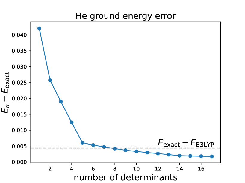
Figure 4. Convergence of MCSCF to the exact ground state energy $E_{\text{exact}}=-2.90372$.

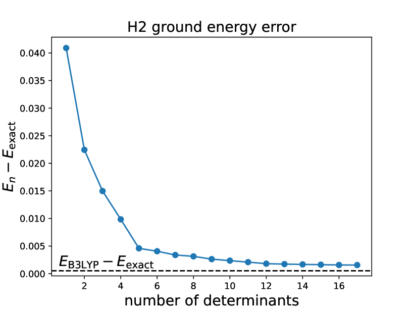
Figure 5. Convergence of MCSCF to the exact ground state energy $E_{\text{exact}}=-1.17447$.

It is worth to notice, that we didn’t rely on any chemical intuition in order to choose proper initial guesses for the two quantum systems we regarded. Instead, we first ran single electron calculations starting with orbitals combining randomly localized gaussian functions. The converged ionic simulations were later used for initialization of the Newton treatment of MCSCF. We follow the same initial guess strategy for the excited states, considered below. Alternatively, one can use spherical harmonics appearing in hydrogen-like atoms. However, it is not clear how this initialization approach could be extended to bigger molecules. Therefore, we stick to the randomized initial calculations.

7. Excited states

The first excited singlet state can be approximated as a sum of $M+1$ closed shell determinants

$$\Psi=\sum_{m=0}^{M}c_{m}\left|m\overline{m}\right\rangle.$$

With the additional constrain, corresponding to the orthogonality of $\Psi$ to the ground state $\Psi_{\text{ground}}$, the new Lagrangian takes the form

$$\mathcal{L}=\frac{1}{4}E-\frac{1}{4}\varepsilon\left(\sum_{m=0}^{M}c_{m}^{2}-1\right)-\frac{1}{2}\sum_{i,j=0}^{M}\varepsilon_{ij}\left(\int\varphi_{i}\varphi_{j}-\delta_{ij}\right)-\frac{1}{2}\lambda\sum_{m,n=0}^{M,M^{\text{gr}}}c_{m}c_{n}^{\text{gr}}\left(\int\varphi_{m}\varphi_{n}^{\text{gr}}\right)^{2}$$

with symmetric matrix coefficients $\varepsilon_{ij}$. It is a function of $\varphi_{0},\ldots,\varphi_{M},\varepsilon,c_{0},\ldots,c_{M},$ $\varepsilon_{ij}$ with $i\leqslant j$ and $\lambda$. We calculate its gradient as follows.

$$\frac{\delta\mathcal{L}}{\delta\varphi_{k}} =c_{k}^{2}h\varphi_{k}+c_{k}\sum_{m=0}^{M}c_{m}J(km)\varphi_{m}-\sum_{m=0}^{M}\varepsilon_{km}\varphi_{m}-\lambda\sum_{n=0}^{M^{\text{gr}}}c_{k}c_{n}^{\text{gr}}\varphi_{n}^{\text{gr}}\int\varphi_{k}\varphi_{n}^{\text{gr}},\quad k=0,\ldots,M.$$ (7.1)

$$\frac{\partial\mathcal{L}}{\partial\varepsilon} =-\frac{1}{4}\left(\sum_{m=0}^{M}c_{m}^{2}-1\right).$$ (7.2)

$$\frac{\partial\mathcal{L}}{\partial c_{k}} =\frac{1}{2}\sum_{m=0}^{M}H_{km}c_{m}-\frac{1}{2}\varepsilon c_{k}-\frac{1}{2}\lambda\sum_{n=0}^{M^{\text{gr}}}c_{n}^{\text{gr}}\left(\int\varphi_{k}\varphi_{n}^{\text{gr}}\right)^{2},\quad k=0,\ldots,M.$$ (7.3)

$$\frac{\partial\mathcal{L}}{\partial\varepsilon_{kk}} =-\frac{1}{2}\left(\left\|\varphi_{k}\right\|^{2}-1\right),\quad k=0,\ldots,M,$$ (7.4)

$$\frac{\partial\mathcal{L}}{\partial\varepsilon_{ij}} =-\int\varphi_{i}\varphi_{j},\quad 0\leqslant i<j\leqslant M.$$ (7.5)

$$\frac{\partial\mathcal{L}}{\partial\lambda} =-\frac{1}{2}\sum_{m,n=0}^{M,M^{\text{gr}}}c_{m}c_{n}^{\text{gr}}\left(\int\varphi_{m}\varphi_{n}^{\text{gr}}\right)^{2}$$ (7.6)

Now let us calculate the Hessian $d\nabla\mathcal{L}$.

$$\sum_{j=0}^{M}\partial_{\varphi_{j}}\frac{\delta\mathcal{L}}{\delta\varphi_{k}}\delta\varphi_{j}=c_{k}^{2}h\delta\varphi_{k}-\sum_{m=0}^{M}\varepsilon_{km}\delta\varphi_{m}+c_{k}\sum_{m=0}^{M}c_{m}\left(J(\delta km)\varphi_{m}+J(k\delta m)\varphi_{m}+J(km)\delta\varphi_{m}\right)\\ -\lambda\sum_{n=0}^{M^{\text{gr}}}c_{k}c_{n}^{\text{gr}}\varphi_{n}^{\text{gr}}\int\delta\varphi_{k}\varphi_{n}^{\text{gr}},$$ (7.7)

where $k=0,\ldots,M.$

$$\frac{\partial}{\partial\varepsilon}\frac{\delta\mathcal{L}}{\delta\varphi_{k}}=0$$

$$\sum_{j=0}^{M}\frac{\partial}{\partial c_{j}}\frac{\delta\mathcal{L}}{\delta\varphi_{k}}\delta c_{j}=2c_{k}\delta c_{k}h\varphi_{k}+\delta c_{k}\sum_{m=0}^{M}c_{m}J(km)\varphi_{m}+c_{k}\sum_{m=0}^{M}\delta c_{m}J(km)\varphi_{m}-\lambda\sum_{n=0}^{M^{\text{gr}}}\delta c_{k}c_{n}^{\text{gr}}\varphi_{n}^{\text{gr}}\int\varphi_{k}\varphi_{n}^{\text{gr}}$$

$$\sum_{0\leqslant i\leqslant j\leqslant M}\frac{\partial}{\partial\varepsilon_{ij}}\frac{\delta\mathcal{L}}{\delta\varphi_{k}}\delta\varepsilon_{ij}=-\sum_{m=0}^{M}\delta\varepsilon_{km}\varphi_{m},$$

where we extended the orbital energy update by symmetry.

$$\frac{\partial}{\partial\lambda}\frac{\delta\mathcal{L}}{\delta\varphi_{k}}\delta\lambda=-\delta\lambda\sum_{n=0}^{M^{\text{gr}}}c_{k}c_{n}^{\text{gr}}\varphi_{n}^{\text{gr}}\int\varphi_{k}\varphi_{n}^{\text{gr}}$$

Summing these equalities we obtain

$$d\frac{\delta\mathcal{L}}{\delta\varphi_{k}}\delta w=c_{k}^{2}h\delta\varphi_{k}-\sum_{m=0}^{M}\varepsilon_{km}\delta\varphi_{m}+c_{k}\sum_{m=0}^{M}c_{m}\left(J(\delta km)\varphi_{m}+J(k\delta m)\varphi_{m}+J(km)\delta\varphi_{m}\right)\\ +2c_{k}\delta c_{k}h\varphi_{k}+\delta c_{k}\sum_{m=0}^{M}c_{m}J(km)\varphi_{m}+c_{k}\sum_{m=0}^{M}\delta c_{m}J(km)\varphi_{m}-\sum_{m=0}^{M}\delta\varepsilon_{km}\varphi_{m}\\ -\lambda\sum_{n=0}^{M^{\text{gr}}}c_{k}c_{n}^{\text{gr}}\varphi_{n}^{\text{gr}}\int\delta\varphi_{k}\varphi_{n}^{\text{gr}}-\lambda\sum_{n=0}^{M^{\text{gr}}}\delta c_{k}c_{n}^{\text{gr}}\varphi_{n}^{\text{gr}}\int\varphi_{k}\varphi_{n}^{\text{gr}}-\delta\lambda\sum_{n=0}^{M^{\text{gr}}}c_{k}c_{n}^{\text{gr}}\varphi_{n}^{\text{gr}}\int\varphi_{k}\varphi_{n}^{\text{gr}}$$ (7.8)

$$d\frac{\partial\mathcal{L}}{\partial\varepsilon}\delta w=-\frac{1}{2}\sum_{m=0}^{M}c_{m}\delta c_{m}$$ (LHS2)

$$\sum_{j=0}^{M}\partial_{\varphi_{j}}\frac{\partial\mathcal{L}}{\partial c_{k}}\delta\varphi_{j}=2c_{k}(\delta k|h|k)+\sum_{m=0}^{M}c_{m}(\delta km|km)+\sum_{m=0}^{M}c_{m}(k\delta m|km)-\lambda\sum_{n=0}^{M^{\text{gr}}}c_{n}^{\text{gr}}\left(\int\varphi_{k}\varphi_{n}^{\text{gr}}\right)\int\delta\varphi_{k}\varphi_{n}^{\text{gr}}$$

$$\frac{\partial}{\partial{\varepsilon}}\frac{\partial\mathcal{L}}{\partial c_{k}}\delta\varepsilon=-\frac{1}{2}\delta\varepsilon c_{k}$$

$$\sum_{j=0}^{M}\frac{\partial}{\partial c_{j}}\frac{\partial\mathcal{L}}{\partial c_{k}}\delta c_{j}=\frac{1}{2}\sum_{m=0}^{M}H_{km}\delta c_{m}-\frac{1}{2}\varepsilon\delta c_{k}$$

$$\frac{\partial}{\partial{\lambda}}\frac{\partial\mathcal{L}}{\partial c_{k}}\delta\lambda=-\frac{1}{2}\delta\lambda\sum_{n=0}^{M^{\text{gr}}}c_{n}^{\text{gr}}\left(\int\varphi_{k}\varphi_{n}^{\text{gr}}\right)^{2}$$

Summing these equalities we obtain

$$d\frac{\partial\mathcal{L}}{\partial c_{k}}\delta w=2c_{k}(\delta k|h|k)+\sum_{m=0}^{M}c_{m}(\delta km|km)+\sum_{m=0}^{M}c_{m}(k\delta m|km)-\frac{1}{2}\delta\varepsilon c_{k}+\frac{1}{2}\sum_{m=0}^{M}H_{km}\delta c_{m}-\frac{1}{2}\varepsilon\delta c_{k}\\ -\lambda\sum_{n=0}^{M^{\text{gr}}}c_{n}^{\text{gr}}\left(\int\varphi_{k}\varphi_{n}^{\text{gr}}\right)\int\delta\varphi_{k}\varphi_{n}^{\text{gr}}-\frac{1}{2}\delta\lambda\sum_{n=0}^{M^{\text{gr}}}c_{n}^{\text{gr}}\left(\int\varphi_{k}\varphi_{n}^{\text{gr}}\right)^{2}$$ (7.9)

Finally,

$$d\frac{\partial\mathcal{L}}{\partial\varepsilon_{kk}}\delta w=-\int\varphi_{k}\delta\varphi_{k},\quad k=0,\ldots,M,$$ (LHS4)

$$d\frac{\partial\mathcal{L}}{\partial\varepsilon_{ij}}\delta w=-\int\delta\varphi_{i}\varphi_{j}-\int\varphi_{i}\delta\varphi_{j},\quad 0\leqslant i<j\leqslant M,$$ (LHS5)

$$d\frac{\partial\mathcal{L}}{\partial\lambda}\delta w=-\sum_{m,n=0}^{M,M^{\text{gr}}}c_{m}c_{n}^{\text{gr}}\left(\int\varphi_{m}\varphi_{n}^{\text{gr}}\right)\int\delta\varphi_{m}\varphi_{n}^{\text{gr}}-\frac{1}{2}\sum_{m,n=0}^{M,M^{\text{gr}}}\delta c_{m}c_{n}^{\text{gr}}\left(\int\varphi_{m}\varphi_{n}^{\text{gr}}\right)^{2}.$$ (LHS6)

The right hand side is $-\nabla\mathcal{L}$. This finishes the detailed description of the Newton equation. Now we want to rewrite it in the self-consistent form, which will be suitable for an iterative procedure.

7.1. Self-consistent form

We rewrite the Newton equation in the form (6.7) where

$$w=(\varphi_{1},\ldots,\varphi_{M},\varepsilon,c_{0},\ldots,\varepsilon_{M-1,M},\lambda)$$

is fixed at each Newton step, as follows.

$$\begin{pmatrix}0&0&\mathbf{c}^{T}\\ 0&0&\mathbf{v}^{T}\\ \mathbf{c}&\mathbf{v}&\varepsilon-H\end{pmatrix}\begin{pmatrix}\delta\varepsilon\\ \delta\lambda\\ \delta\mathbf{c}\end{pmatrix}=\begin{pmatrix}-\frac{1}{2}\left(\sum_{m=0}^{M}c_{m}^{2}-1\right)\\ -\langle\mathbf{c},\mathbf{v}\rangle-2\sum_{m,n=0}^{M,M^{\text{gr}}}c_{m}c_{n}^{\text{gr}}\left(\int\varphi_{m}\varphi_{n}^{\text{gr}}\right)\int\delta\varphi_{m}\varphi_{n}^{\text{gr}}\\ f\end{pmatrix}$$

where $\mathbf{c}=(c_{0},c_{1},\dots,c_{M})^{T}$ and $\mathbf{v}=(v_{0},v_{1},\dots,v_{M})^{T}$ are column vectors with

$$v_{k}=\sum_{n=0}^{M^{\text{gr}}}c_{n}^{\text{gr}}\left(\int\varphi_{k}\varphi_{n}^{\text{gr}}\right)^{2},\quad k=0,\ldots,M,$$

$\varepsilon-H$ is an $(M+1)\times(M+1)$ matrix. Here

$$f_{k}=\sum_{m=0}^{M}H_{km}c_{m}-\varepsilon c_{k}-\lambda v_{k}+4c_{k}(\delta k|h|k)+2\sum_{m=0}^{M}c_{m}(\delta km|km)+2\sum_{m=0}^{M}c_{m}(k\delta m|km)\\ -2\lambda\sum_{n=0}^{M^{\text{gr}}}c_{n}^{\text{gr}}\left(\int\varphi_{k}\varphi_{n}^{\text{gr}}\right)\int\delta\varphi_{k}\varphi_{n}^{\text{gr}},\quad k=0,\ldots,M$$

The matrix $F$ and the Sylvester equation are defined exactly as above. One can compute

$$F_{kj}=c_{k}^{2}(\delta k|h|j)+c_{k}^{2}(k|h|j)-\varepsilon_{kj}+2c_{k}\delta c_{k}(k|h|j)+\sum_{m=0}^{M}c_{k}c_{m}(\delta km+k\delta m|jm)\\ +\sum_{m=0}^{M}\left((c_{k}c_{m}\delta\varphi_{m}+(c_{k}\delta c_{m}+\delta c_{k}c_{m}+c_{k}c_{m})\varphi_{m})\varphi_{j}|km\right)\\ -\lambda c_{k}\sum_{n=0}^{M^{\text{gr}}}c_{n}^{\text{gr}}\int\delta\varphi_{k}\varphi_{n}^{\text{gr}}\int\varphi_{j}\varphi_{n}^{\text{gr}}-(\lambda\delta c_{k}+\delta\lambda c_{k}+\lambda c_{k})\sum_{n=0}^{M^{\text{gr}}}c_{n}^{\text{gr}}\int\varphi_{k}\varphi_{n}^{\text{gr}}\int\varphi_{j}\varphi_{n}^{\text{gr}}$$

for $k,j=0,\ldots,M$.

It is left to precondition the first $M+1$ equations in the Newton system

$$d\frac{\delta\mathcal{L}}{\delta\varphi_{k}}\delta w+\frac{\delta\mathcal{L}}{\delta\varphi_{k}}=0$$

as follows

$$\left(-\frac{c_{k}^{2}}{2}\Delta-\varepsilon_{kk}\right)\delta\varphi_{k}+\left(1+\frac{2\delta c_{k}}{c_{k}}\right)\left(-\frac{c_{k}^{2}}{2}\Delta-\varepsilon_{kk}\right)\varphi_{k}+\left(\frac{2\delta c_{k}}{c_{k}}\varepsilon_{kk}-\delta\varepsilon_{kk}\right)\varphi_{k}\\ +c_{k}^{2}V_{\text{nuc}}\left(\left(1+\frac{2\delta c_{k}}{c_{k}}\right)\varphi_{k}+\delta\varphi_{k}\right)-\sum_{\begin{subarray}{c}m=0\\ m\neq k\end{subarray}}^{M}\left(\varepsilon_{km}\delta\varphi_{m}+\delta\varepsilon_{km}\varphi_{m}+\varepsilon_{km}\varphi_{m}\right)\\ +\delta c_{k}\sum_{m=0}^{M}c_{m}J(km)\varphi_{m}+c_{k}\sum_{m=0}^{M}\delta c_{m}J(km)\varphi_{m}+c_{k}\sum_{m=0}^{M}c_{m}J(km)(\varphi_{m}+\delta\varphi_{m})\\ +c_{k}\sum_{m=0}^{M}c_{m}\left(J(\delta km)\varphi_{m}+J(k\delta m)\varphi_{m}\right)\\ -\lambda c_{k}\sum_{n=0}^{M^{\text{gr}}}c_{n}^{\text{gr}}\varphi_{n}^{\text{gr}}\int\delta\varphi_{k}\varphi_{n}^{\text{gr}}-(\lambda\delta c_{k}+\delta\lambda c_{k}+\lambda c_{k})\sum_{n=0}^{M^{\text{gr}}}c_{n}^{\text{gr}}\varphi_{n}^{\text{gr}}\int\varphi_{k}\varphi_{n}^{\text{gr}}=0$$

Finally, we arrive to (6.8) with

$$\mathfrak{F}_{k}=\left(\frac{2\delta c_{k}}{c_{k}}\varepsilon_{kk}-\delta\varepsilon_{kk}\right)\varphi_{k}+c_{k}^{2}V_{\text{nuc}}\left(\left(1+\frac{2\delta c_{k}}{c_{k}}\right)\varphi_{k}+\delta\varphi_{k}\right)\\ -\sum_{\begin{subarray}{c}m=0\\ m\neq k\end{subarray}}^{M}\left(\varepsilon_{km}\delta\varphi_{m}+\delta\varepsilon_{km}\varphi_{m}+\varepsilon_{km}\varphi_{m}\right)+\sum_{m=0}^{M}J(km)\left((\delta c_{k}c_{m}+c_{k}\delta c_{m}+c_{k}c_{m})\varphi_{m}+c_{k}c_{m}\delta\varphi_{m}\right)\\ +c_{k}\sum_{m=0}^{M}c_{m}\left(J(\delta km)\varphi_{m}+J(k\delta m)\varphi_{m}\right)\\ -\lambda c_{k}\sum_{n=0}^{M^{\text{gr}}}c_{n}^{\text{gr}}\varphi_{n}^{\text{gr}}\int\delta\varphi_{k}\varphi_{n}^{\text{gr}}-(\lambda\delta c_{k}+\delta\lambda c_{k}+\lambda c_{k})\sum_{n=0}^{M^{\text{gr}}}c_{n}^{\text{gr}}\varphi_{n}^{\text{gr}}\int\varphi_{k}\varphi_{n}^{\text{gr}}$$

and the convolution operator $R_{k}$ is defined as above. This finishes the description of $\mathbb{F}_{k}$ in (6.7).

It is left to describe the excited Löwdin step (see Appendix), and the CI coefficient minimization:

$$PHPc=\varepsilon c,$$

where the projection has the elements:

$$P_{km}=\delta_{km}-\frac{v_{k}v_{m}}{\left\|v\right\|^{2}}.$$

7.2. Numerics

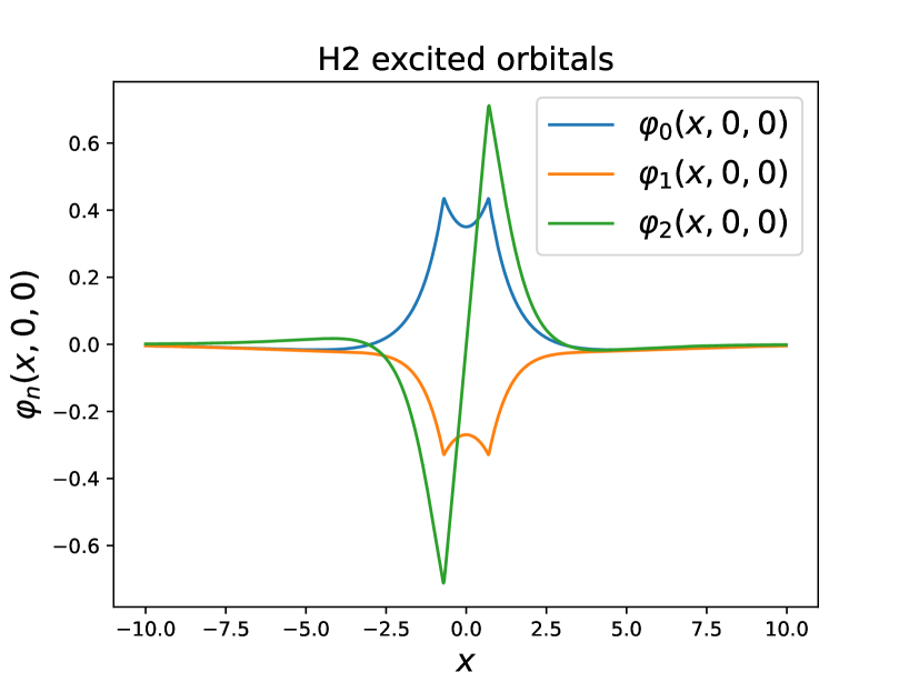
Figure 6. Three determinants excited state of the hydrogen molecule with the coefficients $c_{0}=0.76103,c_{1}=-0.64796$ and $c_{2}=-0.03128$, accordingly. The corresponding energy is $-0.68989$.

For He atom high accuracy excited states were computed in [3]. The first excited singlet state has the energy $-2.14597404605441741580502897546192$, that serves as a reference. Impressively, our method gives the energy $-2.14350$ for two determinants associated to coefficients $c_{0}=0.75880,c_{1}=-0.65132$ and $M^{\text{gr}}=5$ corresponding to 6 configurations in the ground state.

For H2 molecule we calculate the first closed shell excited state at the same internuclear distance $R_{\text{nuc}}=1.4010784$ as above. Using 6 configurations in the ground state for the constrain, we report the energy $-0.68844$ for two configurations with $c_{0}=0.76135,c_{1}=-0.64834$ and the energy $-0.69028$ for 5 determinants with $c_{0}=0.76125,c_{1}=-0.64732,c_{2}=-0.03140,c_{3}=0.01669,c_{4}=0.01461$. The orbitals can be observed in Figure 6. In this case we do not have a high precision energy value, which one could use as a reference, but some close values were reported in [7, 18].

Appendix A Löwdin transformation

Given a set of linearly independent orbitals $\phi_{1},\ldots,\phi_{N}\in L^{2}$ and a non-zero vector $(a_{1},\ldots,a_{N})\in\mathbb{R}^{N}$, we want to transform them in a way that the new orbitals $\psi_{1},\ldots,\psi_{N}\in L^{2}$ and coefficients $b_{1},\ldots,b_{N}\in\mathbb{R}$ satisfy a particular constrain, while been kept as close as possible to the original ones. The latter we formalize as the minimization of the distance

$$\sum_{n=1}^{N}\left\|\psi_{n}-\phi_{n}\right\|^{2}+\sum_{n=1}^{N}\left|b_{n}-a_{n}\right|^{2}.$$ (1.1)

A.1. Ground state constrain

We impose the following conditions

$$\langle\psi_{k},\psi_{n}\rangle=\delta_{kn},\quad\sum_{n}b_{n}^{2}=1$$

on the unknowns $\psi_{n},b_{n}$, which naturally appear in the ground state MCSCF problem. And we want to minimize the distance (1.1) to the given fixed orbitals $\phi_{n}$ and coefficients $a_{n}$. It turns out that the well-known symmetric Löwdin orthonormalisation is the unique solution of this minimization problem [8]. Here we re-derive it making use of the Lagrangian formalism. Firstly, one may easily notice that accounting for the imposed constrain the objective functional can be simplified. In other words, the minimization problem is equivalent to the maximization of

$$\mathcal{F}(\psi_{1},\ldots,\psi_{N},b_{1},\ldots,b_{N})=\sum_{n=1}^{N}\left(\langle\phi_{n},\psi_{n}\rangle+a_{n}b_{n}\right),$$

as pointed out in [15], where one can also find an alternative instructive derivation.

Introducing the Lagrangian

$$\mathcal{L}=\sum_{n=1}^{N}\left(\langle\phi_{n},\psi_{n}\rangle+a_{n}b_{n}\right)-\frac{1}{2}\sum_{i,j=1}^{N}\varepsilon_{ij}\left(\langle\psi_{i},\psi_{j}\rangle-\delta_{ij}\right)-\frac{1}{2}\beta\left(\sum_{n=1}^{N}b_{n}^{2}-1\right)$$

with symmetric matrix $\varepsilon=(\varepsilon_{ij})$ and computing its gradient, we arrive to the equations

$$\phi_{k}-\sum_{n=1}^{N}\varepsilon_{kn}\psi_{n}=0$$

$$a_{k}-\beta b_{k}=0$$

describing stationary points of the functional $\mathcal{L}(\psi_{1},\ldots,\psi_{N},b_{1},\ldots,b_{N})$. The obtained equations on orbitals are decoupled from the equations on the coefficients, because they are restricted independently. The first system implies that the original orbitals $\phi_{1},\ldots,\phi_{N}$ belong to the span of $\psi_{1},\ldots,\psi_{N}$. Therefore, recalling that by the assumption the original orbitals $\phi_{1},\ldots,\phi_{N}$ are linearly independent we deduce that the matrix $\varepsilon$ is invertible. The inverse matrix $\varepsilon^{-1}$ is also symmetric, since the corresponding Lagrange multipliers were introduced symmetrically. Thus

$$\psi_{m}=\sum_{k=1}^{N}\left(\varepsilon^{-1}\right)_{mk}\phi_{k}$$

and from the second system we obtain

$$b_{k}=\frac{1}{\beta}a_{k}.$$

Note that $\beta$ cannot be zero, otherwise it would violate the non-zero condition imposed on the vector $(a_{1},\ldots,a_{N})$. Finally, the Lagrange multipliers can be found from the ground state constrain as

$$\delta_{mn}=\langle\psi_{m},\psi_{n}\rangle=\sum_{k,l=1}^{N}\left(\varepsilon^{-1}\right)_{mk}\left(\varepsilon^{-1}\right)_{nl}\langle\phi_{k},\phi_{l}\rangle=\left(\varepsilon^{-1}S\varepsilon^{-T}\right)_{mn}=\left(\varepsilon^{-1}S\varepsilon^{-1}\right)_{mn},$$

with $S_{kl}=\langle\phi_{k},\phi_{l}\rangle$, and

$$1=\left\|b\right\|^{2}=\frac{1}{\beta^{2}}\left\|a\right\|^{2}.$$

It leads to $\varepsilon^{2}=S$ and $\beta^{2}=\left\|a\right\|^{2}$. As we will shortly see, $\mathcal{F}$ achieves a maximum, provided the signs of $\varepsilon$ and $\beta$ are set as $\varepsilon=\sqrt{S}$ and $\beta=\left\|a\right\|$. The obtained transformation

$$\psi=S^{-1/2}\phi,\quad b=a/\left\|a\right\|$$ (1.2)

is the standard Löwdin orthogonalisation.

It is left to show that the obtained stationary point (1.2) is indeed a maximum. By the Cauchy–Schwarz inequality

$$\sum_{n=1}^{N}a_{n}b_{n}\leqslant\left\|a\right\|\left\|b\right\|=\left\|a\right\|$$

for any real vector $b$ with $\left\|b\right\|=1$. Moreover, the equality is achieved if and only if $a,b$ are linearly dependent, which in this case is equivalent to $b=a/\left\|a\right\|$. It shows that the euclidean part of $\mathcal{F}$ is strictly bounded from above by its value at the stationary point (1.2). The corresponding functional inner product part of $\mathcal{F}$ is estimated, firstly, by restricting to the span of the original orbitals $\phi_{1},\ldots,\phi_{N}$. In other words, we suppose that the new orthonormalised functions $\psi_{1},\ldots,\psi_{N}$ can be obtained by a matrix transformation $\psi=\alpha\phi$ of coordinates $\phi_{1},\ldots,\phi_{N}$. Obviously, the matrix $\alpha$ is invertible. From the normalization constrain we deduce

$$S=\alpha^{-1}\alpha^{-T}$$

and so the Lagrange multiplier matrix $\varepsilon$ is related to $\alpha$ as

$$\varepsilon=\sqrt{S}=\sqrt{\alpha^{-1}\alpha^{-T}}=\left|\alpha^{-1}\right|.$$

Therefore,

$$\sum_{n=1}^{N}\langle\phi_{n},\psi_{n}\rangle=\sum_{n,m=1}^{N}\alpha_{n,m}S_{n,m}=\operatorname{tr}(\alpha S)=\operatorname{tr}\left(\alpha^{-1}\right)\leqslant\left\|\alpha^{-1}\right\|_{1}=\operatorname{tr}\left|\alpha^{-1}\right|\\ =\operatorname{tr}\varepsilon=\operatorname{tr}(\varepsilon^{-1}S)=\sum_{n=1}^{N}\left\langle\phi_{n},\left(\varepsilon^{-1}\phi\right)_{n}\right\rangle,$$

where we have used the well-known relation for nuclear operators, in this particular case for the matrix $\alpha^{-1}$, between the trace and the norm [4]. It proves the statement in the span of the original orbitals.

Finally, in the general case one can project each orbital $\psi_{k}$ onto $\operatorname{Span}\phi$ and its orthogonal complement with the projections $P$ and $Q$, correspondingly, as

$$\psi_{k}=P\psi_{k}+Q\psi_{k},$$

where the functions $P\psi_{k}$ can be obtained from the transformation $P\psi=\alpha\phi.$ Thus the orthonormalisation constrain

$$\delta_{nm}=\langle\psi_{n},\psi_{m}\rangle=\sum_{k,l}\alpha_{nk}\alpha_{ml}S_{kl}+\langle Q\psi_{n},Q\psi_{m}\rangle$$

leads to

$$\mathds{1}=\alpha S\alpha^{T}+F$$

with the overlap matrix $F$ satisfying $0\leqslant F\leqslant\mathds{1}$. Indeed, for any vector $x\in\mathbb{R}^{N}$ we have

$$\langle Fx,x\rangle=\sum_{n,m}F_{nm}x_{n}x_{m}=\sum_{n,m}\langle Q\psi_{n},Q\psi_{m}\rangle x_{n}x_{m}=\left\|Q\left(\sum_{n}x_{n}\psi_{n}\right)\right\|^{2}\leqslant\left\|\sum_{n}x_{n}\psi_{n}\right\|^{2}=\left\|x\right\|^{2}$$

implying the bounds on $F$. Hence

$$\varepsilon^{2}=S=\alpha^{-1}(\mathds{1}-F)\alpha^{-T}$$

and so

$$\varepsilon=\sqrt{S}=\sqrt{\alpha^{-1}\sqrt{\mathds{1}-F}\left(\alpha^{-1}\sqrt{\mathds{1}-F}\right)^{T}}=\left|\alpha^{-1}\sqrt{\mathds{1}-F}\right|.$$

As above we estimate

$$\sum_{n=1}^{N}\langle\phi_{n},\psi_{n}\rangle=\sum_{n=1}^{N}\langle\phi_{n},P\psi_{n}\rangle=\operatorname{tr}(\alpha S)=\operatorname{tr}\left(\alpha^{-1}(\mathds{1}-F)\right)\leqslant\left\|\alpha^{-1}(\mathds{1}-F)\right\|_{1}\\ \leqslant\left\|\alpha^{-1}\sqrt{\mathds{1}-F}\right\|_{1}\left\|\sqrt{\mathds{1}-F}\right\|\leqslant\operatorname{tr}\varepsilon=\operatorname{tr}(\varepsilon^{-1}S)=\sum_{n=1}^{N}\left\langle\phi_{n},\left(\varepsilon^{-1}\phi\right)_{n}\right\rangle,$$

where we used the norm estimate $\left\|\sqrt{\mathds{1}-F}\right\|\leqslant 1$ following from

$$\left\|\sqrt{\mathds{1}-F}x\right\|^{2}=\langle(\mathds{1}-F)x,x\rangle\leqslant\left\|x\right\|^{2}$$

holding true for any vector $x\in\mathbb{R}^{N}$, obviously. This completes the proof of the minimization property of the Löwdin transform (1.2). For an alternative rigorous exposition we refer to [8].

A.2. Excited state constrain

We want to maximize

$$\sum_{n=1}^{N}\left(\langle\phi_{n},\psi_{n}\rangle+a_{n}b_{n}\right)$$

where $\phi_{n},a_{n}$ with $n=1,\ldots,N$ are fixed given values. The unknowns $\psi_{n},b_{n}$ satisfy the following constraints

$$\langle\psi_{k},\psi_{n}\rangle=\delta_{kn},\quad\sum_{n}b_{n}^{2}=1$$

and

$$\sum_{n=1}^{N}\sum_{m=1}^{M}b_{n}c_{m}\langle\psi_{n},g_{m}\rangle^{2}=0,$$

where $g_{m},c_{m}$ with $m=1,\ldots,M$ are fixed given and normalized as

$$\langle g_{l},g_{m}\rangle=\delta_{lm},\quad\sum_{m}c_{m}^{2}=1.$$

We introduce the Lagrangian

$$\mathcal{L}=\sum_{n=1}^{N}\left(\langle\phi_{n},\psi_{n}\rangle+a_{n}b_{n}\right)-\frac{1}{2}\sum_{i,j=1}^{N}\varepsilon_{ij}\left(\langle\psi_{i},\psi_{j}\rangle-\delta_{ij}\right)-\frac{1}{2}\beta\left(\sum_{n=1}^{N}b_{n}^{2}-1\right)-\frac{1}{2}\lambda\sum_{n=1}^{N}\sum_{m=1}^{M}b_{n}c_{m}\langle\psi_{n},g_{m}\rangle^{2}$$

with symmetric matrix $\varepsilon=(\varepsilon_{ij})$ and compute its gradient

$$\frac{\delta\mathcal{L}}{\delta\psi_{k}}=\phi_{k}-\sum_{n=1}^{N}\varepsilon_{kn}\psi_{n}-\lambda b_{k}\sum_{m=1}^{M}c_{m}\langle\psi_{k},g_{m}\rangle g_{m}$$

$$\frac{\partial\mathcal{L}}{\partial b_{k}}=a_{k}-\beta b_{k}-\frac{1}{2}\lambda\sum_{m=1}^{M}c_{m}\langle\psi_{k},g_{m}\rangle^{2}$$

Thus the unknowns $\psi_{n},b_{n}$, the symmetric matrix $\varepsilon=(\varepsilon_{ij})$ and scalars $\beta,\lambda$ satisfy the following system

$$\phi_{k}-\sum_{n=1}^{N}\varepsilon_{kn}\psi_{n}-\lambda b_{k}\sum_{m=1}^{M}c_{m}\langle\psi_{k},g_{m}\rangle g_{m} =0$$

$$a_{k}-\beta b_{k}-\frac{1}{2}\lambda\sum_{m=1}^{M}c_{m}\langle\psi_{k},g_{m}\rangle^{2} =0$$

$$\langle\psi_{i},\psi_{j}\rangle =\delta_{ij}$$

$$\sum_{n=1}^{N}b_{n}^{2} =1$$

$$\sum_{n=1}^{N}\sum_{m=1}^{M}b_{n}c_{m}\langle\psi_{n},g_{m}\rangle^{2} =0$$

It is possible to reduce the problem to the finite dimensional space by searching for $\psi_{n}$ in the span of $\phi_{n},g_{m}$ as

$$\psi_{k}=\sum_{n=1}^{N}A_{kn}\phi_{n}+\sum_{m=1}^{M}B_{km}g_{m}.$$

Therefore we need to find the matrices $A,B,\varepsilon$ and scalars $\beta,\lambda$. Define

$$\Phi_{kl}=\langle\phi_{k},\phi_{l}\rangle,\quad k,l=1,\ldots,N$$

$$G_{ml}=\langle g_{m},\phi_{l}\rangle,\quad m=1,\ldots,M,\quad l=1,\ldots,N$$

These overlap matrices are fixed and given. Then

$$\langle\psi_{k},g_{m}\rangle=\sum_{n=1}^{N}A_{kn}G_{mn}+B_{km}$$

and

$$\langle\psi_{k},\phi_{l}\rangle=\sum_{n=1}^{N}A_{kn}\Phi_{nl}+\sum_{m=1}^{M}B_{km}G_{ml}.$$

We want to maximize

$$\sum_{k=1}^{N}\left(\langle\phi_{k},\psi_{k}\rangle+a_{k}b_{k}\right)=\sum_{k=1}^{N}\left(\sum_{n=1}^{N}A_{kn}\Phi_{nk}+\sum_{m=1}^{M}B_{km}G_{mk}+a_{k}b_{k}\right)$$

The orthonormality constrain is imposed on the overlap:

$$\langle\psi_{k},\psi_{l}\rangle=\sum_{n,n^{\prime}=1}^{N}A_{kn}A_{ln^{\prime}}\Phi_{nn^{\prime}}+\sum_{m=1}^{M}B_{km}B_{lm}+\sum_{n=1}^{N}\sum_{m=1}^{M}(A_{kn}B_{lm}+A_{ln}B_{km})G_{mn}.$$

Finally, orthogonality to the ground state reads

$$\sum_{n=1}^{N}\sum_{m=1}^{M}b_{n}c_{m}\left(\sum_{n^{\prime}=1}^{N}A_{nn^{\prime}}G_{mn^{\prime}}+B_{nm}\right)^{2}=0$$

The optimization was implemented using the scipy.optimize.minimize routine with method SLSQP, subject to nonlinear equality constraints: orthonormality of $\psi_{n}$, unit norm of the scalar vector $b_{n}$, and a bilinear orthogonality condition involving the functions $g_{m}$. We set the initial guess as

$$A^{(0)}=I_{N},\quad B^{(0)}=0,\quad\text{and}\quad\|b^{(0)}\|=1.$$

To ensure convergence, we increased the maximum number of iterations to 10,000 and reduced the function tolerance to $10^{-12}$.

Appendix B Spherical harmonics

$$A_{m}(x,y)=\sum_{p=0}^{m}\begin{pmatrix}m\\ p\end{pmatrix}x^{p}y^{m-p}\cos\left((m-p)\frac{\pi}{2}\right)$$

$$B_{m}(x,y)=\sum_{p=0}^{m}\begin{pmatrix}m\\ p\end{pmatrix}x^{p}y^{m-p}\sin\left((m-p)\frac{\pi}{2}\right)$$

$$\Pi_{l}^{m}(z)=\left(\frac{(l-m)!}{(l+m)!}\right)^{1/2}\sum_{k=0}^{\lfloor(l-m)/2\rfloor}(-1)^{k}2^{-l}\begin{pmatrix}l\\ k\end{pmatrix}\begin{pmatrix}2l-2k\\ l\end{pmatrix}\frac{(l-2k)!}{(l-2k-m)!}r^{2k}z^{l-2k-m}$$

Then for $m>0$ we have

$$r^{l}\begin{pmatrix}Y_{l,m}\\ Y_{l,-m}\end{pmatrix}=\sqrt{\frac{2l+1}{2\pi}}\Pi_{l}^{m}(z)\begin{pmatrix}A_{m}\\ B_{m}\end{pmatrix}$$

and for $m=0$:

$$r^{l}Y_{l,0}=\sqrt{\frac{2l+1}{4\pi}}\Pi_{l}^{0}(z)$$

Declarations

The CRediT taxonomy of contributor roles [2, 6] is applied. The “Investigation” role also includes the “Methodology”, “Software”, and “Validation” roles. The “Analysis” role also includes the “Formal analysis” and “Visualization” roles. The “Funding acquisition” role also includes the “Resources” role. The contributor roles are visualized in the following authorship attribution matrix, as suggested in Ref. [1].

Table 1. Levels of contribution: major, minor.

	ED	RVS	LF
Conceptualization
Investigation
Data curation
Analysis
Supervision
Writing – original draft
Writing – revisions
Funding acquisition
Project administration

Acknowledgments. We acknowledge support from the Research Council of Norway through its Centres of Excellence scheme (Hylleraas centre, 262695), through the FRIPRO grant ReMRChem (324590), and from NOTUR – The Norwegian Metacenter for Computational Science through grant of computer time (nn14654k).

References

• [1] Researchers are embracing visual tools to give fair credit for work on papers. https://www.natureindex.com/news-blog/researchers-embracing-visual-tools-contribution-matrix-give-fair-credit-authors-scientific-papers. Accessed: 2021-5-3.
• [2] Allen, L., Scott, J., Brand, A., Hlava, M., and Altman, M. Publishing: Credit where credit is due. Nature 508 (2014), 312–313.
• [3] Aznabaev, D. T., Bekbaev, A. K., and Korobov, V. I. Nonrelativistic energy levels of helium atoms. Phys. Rev. A 98 (Jul 2018), 012510.
• [4] Birman, M. S., and Solomjak, M. Z. Spectral Theory of Self-Adjoint Operators in Hilbert Space, vol. 5 of Mathematics and Its Applications (Soviet Series). Springer Science+Business Media, Dordrecht, 1987. Translated from the Russian by S. Khrushchëv and V. Peller.
• [5] Bischoff, F. A. Chapter one - computing accurate molecular properties in real space using multiresolution analysis. In State of The Art of Molecular Electronic Structure Computations: Correlation Methods, Basis Sets and More, L. U. Ancarani and P. E. Hoggan, Eds., vol. 79 of Advances in Quantum Chemistry. Academic Press, 2019, pp. 3–52.
• [6] Brand, A., Allen, L., Altman, M., Hlava, M., and Scott, J. Beyond authorship: attribution, contribution, collaboration, and credit. Learn. Publ. 28 (2015), 151–155.
• [7] Cancès, É., Galicher, H., and Lewin, M. Computing electronic structures: A new multiconfiguration approach for excited states. Journal of Computational Physics 212, 1 (2006), 73–98.
• [8] Carlson, B. C., and Keller, J. M. Orthogonalization procedures and the localization of wannier functions. Phys. Rev. 105 (Jan 1957), 102–103.
• [9] Frediani, L., Fossgaard, E., Flå, T., and Ruud, K. Fully adaptive algorithms for multivariate integral equations using the non-standard form and multiwavelets with applications to the poisson and bound-state helmholtz kernels in three dimensions. Molecular Physics 111, 9-11 (2013), 1143–1160.
• [10] Harrison, R. J., Fann, G. I., Yanai, T., and Beylkin, G. Multiresolution quantum chemistry in multiwavelet bases. In Proceedings of the 2003 International Conference on Computational Science (Berlin, Heidelberg, 2003), ICCS’03, Springer-Verlag, p. 103–110.
• [11] Harrison, R. J., Fann, G. I., Yanai, T., Gan, Z., and Beylkin, G. Multiresolution quantum chemistry: Basic theory and initial applications. The Journal of Chemical Physics 121, 23 (11 2004), 11587–11598.
• [12] Helgaker, T., Jørgensen, P., and Olsen, J. Molecular Electronic-Structure Theory. Wiley, 2000.
• [13] Jensen, S. R., Saha, S., Flores-Livas, J. A., Huhn, W., Blum, V., Goedecker, S., and Frediani, L. The elephant in the room of density functional theory calculations. The Journal of Physical Chemistry Letters 8, 7 (2017), 1449–1457. PMID: 28291362.
• [14] Kolos, W., and Wolniewicz, L. Improved theoretical ground‐state energy of the hydrogen molecule. The Journal of Chemical Physics 49, 1 (07 1968), 404–410.
• [15] Mayer, I. On löwdin’s method of symmetric orthogonalization. International Journal of Quantum Chemistry 90, 1 (2002), 63–65.
• [16] Nakashima, H., and Nakatsuji, H. Solving the schrödinger equation for helium atom and its isoelectronic ions with the free iterative complement interaction (ici) method. The Journal of Chemical Physics 127, 22 (12 2007), 224104.
• [17] Sims, J. S., and Hagstrom, S. A. High precision variational calculations for the born-oppenheimer energies of the ground state of the hydrogen molecule. The Journal of Chemical Physics 124, 9 (03 2006), 094101.
• [18] Siłkowski, M., Zientkiewicz, M., and Pachucki, K. Chapter Twelve - Accurate Born-Oppenheimer potentials for excited $\Sigma+$ states of the hydrogen molecule, vol. 83 of Advances in Quantum Chemistry. Academic Press, 2021, pp. 255–267.
• [19] Szabo, A., and Ostlund, N. S. Modern Quantum Chemistry: Introduction to Advanced Electronic Structure Theory, revised ed. Dover Publications, New York, 1989. Revised Edition.
• [20] Tantardini, C., Dinvay, E., Pitteloud, Q., Gerez S., G. A., Jensen, S. R., Wind, P., Remigio, R. D., and Frediani, L. Advancements in quantum chemistry using multiwavelets: Theory, implementation, and applications. In preparation, 2024.
• [21] Yanai, T., Fann, G. I., Gan, Z., Harrison, R. J., and Beylkin, G. Multiresolution quantum chemistry in multiwavelet bases: Analytic derivatives for Hartree–Fock and density functional theory. The Journal of Chemical Physics 121, 7 (2004), 2866–2876.