Distributed Composite Optimization with Sub-Weibull Noises

Abstract

With the rapid development of multi-agent distributed optimization (MA-DO) theory over the past decade, the distributed stochastic gradient method (DSGM) occupies an important position. Although the theory of different DSGMs has been widely established, the main-stream results of existing work are still derived under the condition of light-tailed stochastic gradient noises. Increasing recent examples from various fields, indicate that, the light-tailed noise model is overly idealized in many practical instances, failing to capture the complexity and variability of noises in real-world scenarios, such as the presence of outliers or extreme values from data science and statistical learning. To address this issue, we propose a new DSGM framework that incorporates stochastic gradients under sub-Weibull randomness. We study a distributed composite stochastic mirror descent scheme with sub-Weibull gradient noise (DCSMD-SW) for solving a distributed composite optimization (DCO) problem over the time-varying multi-agent network. By investigating sub-Weibull randomness in DCSMD for the first time, we show that the algorithm is applicable in common heavy-tailed noise environments while also guaranteeing good convergence properties. We comprehensively study the convergence performance of DCSMD-SW. Satisfactory high probability convergence rates are derived for DCSMD-SW without any smoothness requirement. The work also offers a unified analysis framework for several critical cases of both algorithms and noise environments.

Keywords: distributed optimization, composite objective, sub-Weibull, heavy-tail, stochastic gradient, mirror descent

1 Introduction

Over the past decade, theory of multi-agent distributed optimization (MA-DO) has experienced explosive development, leading to a multitude of MA-DO algorithms that invigorate and inspire the advancement of the intelligent society ([1]-[22]). DO algorithms have been utilized in various application domains of science and technology, including for example, Internet of Things [2], wireless cellular network [3], data-driven machine learning [4], power system [5], smart grid [6].

A typical characteristic of MA-DO is that agents collaboratively address the optimization problem through effective communication of information between themselves and their neighbors. A common problem framework in MA-DO involves minimizing a global objective function, which can be represented as the sum of several local objective cost or loss functions defined on some appropriate decision domains. Around this core problem framework, the issues explored in DO can often be further categorized based on the convexity characteristics of the objective function, as well as the level of regularity of the objective functions and the constraints of the decision region. These categories typically include distributed convex/non-convex/strongly convex optimization, distributed smooth/non-smooth optimization, and distributed constrained/unconstrained optimization. Originating from the work [1], there have been numerous groundbreaking advancements on the formulation of DO algorithms for solving the aforementioned typical problem frameworks over the past decade. These include some fundamental DO approaches, for example, distributed subgradient approach (e.g. [1]), distributed dual-averaging approach (e.g. [7]), distributed subgradient-push approach (e.g. [8]), distributed mirror descent approach (e.g. [9]), distributed primal-dual approach (e.g. [10]).

This paper primarily concentrates on the study of consensus-based DSGM. Classical SGD has a lengthy history, while DSGMs began to evolve concurrently with the development of distributed subgradient methods (see [11]). Recently, many powerful DSGMs have garnered widespread attention (see. e.g. [2], [7], [9], [11], [12], [13], [20], [22], [26], [27], [30]). DSGMs involve algorithms that incorporate randomness of (sub)gradient in their search for optimal solutions. Unlike deterministic methods that follow a fixed path, DSGMs can explore the solution space more broadly, potentially avoiding local minima. This flexibility allows them to better navigate complex landscapes, making them effective for large-scale optimization problems.

In DSGMs, the type of stochastic noise is crucial in the formulation of the stochastic gradient. Different noise characteristics can significantly influence the convergence behavior and performance of DO algorithms. In the early development of DSGMs, gradient noise was typically assumed to have a bounded variance, and the corresponding theoretical framework aimed to achieve expected convergence bounds and rates. Meanwhile, sub-Gaussian distribution is often used in formulating stochastic gradient model. However, an increasing number of instances in machine learning and statistical learning demonstrate that light-tailed noise model such as sub-Gaussian noise is overly idealized for describing the stochastic environment of learning systems (see e.g. [23], [24]) and they often fall short in capturing the complexity and variability of noise in many real-world scenarios, particularly in the presence of outliers or extreme values commonly encountered in machine learning, statistical learning and data science (e.g. [27]-[29]). Moreover, it is quite common that the deep-neural-network-based data science and statistical learning scenarios often exhibit heavy-tailed noises (see e.g. [28]) and their relevant noise environments are better characterized by heavier tailed noise. Hence, it is sensible to develop convergence theory for DO in scenarios characterized by heavier tailed gradient noise.

In existing literature, the studies on MA-DO and its related distributed Nash equilibrium seeking under heavy-tailed noise have only very recently begun to attract attention (e.g. [20], [21], [30]). Moreover, existing findings in this direction remain severely limited. We observe that existing work on DSGMs with heavy-tailed noise primarily focuses on scenarios where the noise possesses lower-order moments. In such extreme cases, despite the introduction of techniques like clipping or normalization, the convergence performance is clearly worse than the optimal or suboptimal rates. This fact drives us to seek a scenario where the stochastic gradient model in the DSGM exhibits the characteristics of heavy-tailed noise (at least encompassing a series of important noise models such as sub-Gaussian and sub-exponential noise), while also achieving significantly better convergence performance than the existing results on DSGMs under heavy-tailed noises. To this end, in this paper, we study DSGM with stochastic gradient modeled by the sub-Weibull noises. Sub-Weibull noise is a type of random noise characterized by exponentially decaying tails, as nicely discussed in the existing optimization and learning literature [31]-[36], which provide inspiring insights. The sub-Weibull distribution can be viewed as a nice intermediate heavy-tailed noise model, heavier than sub-Gaussian noise and lighter than bounded $p$-moment noise for $p\in(0,2)$. It is noteworthy that the high probability convergence theory has not yet been explored for DSGMs with sub-Weibull stochastic gradient noise in the context of MA-DCO. This presents a promising opportunity to establish high probability convergence theory for some classic DSGMs under sub-Weibull noises. This work aims to fill this gap and present an initial exploration into the theoretical study of time-varying MA-DCO within the framework of sub-Weibull randomness.

In this work, we focus on the multi-agent distributed composite convex optimization problem over a time-varying muti-agent system. We study a distributed composite stochastic mirror descent (DCSMD-SW) algorithm that is utilized for solving the problem in the environment of sub-Weibull randomness. Each agent makes decisions solely based on the sub-Weibull gradient noise estimate of its associated local objective function and the state information received from its neighbors at the corresponding time instant. Distributed (stochastic) mirror descent algorithm has been thriving for over a decade (e.g. [9], [12]-[18], [19]), based on bounded second moment condition of the stochastic gradient, the convergence performance in expectation has become the dominant form of main result expression in this research branch. However, the characterization of expected convergence forms has shown evident shortcomings in many learning and optimization scenarios. Because convergence in expectation indicates the iterate scheme has to perform many times to ensure the convergence performance of the algorithm. Such results are insufficient to meet the demands of many modern computational systems that require convergence to be achieved in a single round. To overcome such issues, this paper will provide a new high probability convergence DCSMD-SW framework under heavy-tailed sub-Weibull noise environment.

We summarize the main contribution of this work:
A In this work, sub-Weibull stochastic gradient noise is investigated for the first time in the literature of multi-agent distributed composite optimization. We show that, for any confidence level $0<\delta<1$, DCSMD-SW is able to achieve an high probability convergence rate of $\mathcal{O}(\left(\log\frac{T}{\delta}\right)^{2\theta}\frac{(\log T)^{2}}{\sqrt{T}}+\left(\log\frac{1}{\delta}\right)^{2}\left(\log\frac{T}{\delta}\right)^{2\max\{0,\theta-1\}}\frac{1}{\sqrt{T}})$, where $\theta\geq 1/2$ is the sub-Weibull noise tail parameter. We also show that, under a known time horizon $T$, via a constant stepsize strategy, we can achieve a $\mathcal{O}(\left(\log\frac{T}{\delta}\right)^{2\theta}\frac{1}{\sqrt{T}})$ high probability rate. This is also the first time that explicit high-probability convergence rates have been obtained in MA-DCO under a sub-Weibull noise environment (optimal only up to poly-logarithmic factor). Additionally, this work clearly demonstrates how sub-Weibull noise affects information communication among nodes in the multi-agent system. Importantly, our framework does not require any extra truncation techniques, such as gradient clipping or normalization, which can potentially complicate parameter tuning for the algorithm in practice.

B The high-probability convergence rate of DCSMD-SW is derived without assuming any smoothness or strong convexity, in contrast to previous works that require $L$-smoothness condition or strongly convex condition. This makes our convergence theory applicable to a broader range of functions, allowing for wider use in systems science and machine learning. Moreover, due to the flexible selection of Bregman divergence and local composite regularization functions, our DCSMD-SW analysis framework can degenerate into some crucial distributed algorithms with sub-Weibull randomness such as distributed SGD (DSGD-SW) and distributed stochastic entropic descent algorithm (DSED-SW). Although the high probability convergence rates of these algorithms in sub-Weibull gradient noise environments have not been studied independently, their high-probability convergence rates have been directly obtained as a special case of this work. Thus, our findings offer a unified high-probability convergence framework for these key distributed decentralized algorithms with sub-Weibull noises.

C In existing research on DMD for convex optimization e.g. [9], [12]-[18], the convergence analysis essentially relies on the boundedness of the decision space, which is a key technical assumption. Our work successfully eliminates this requirement, enabling all results to be applicable to unbounded decision domains, including cases of unconstrained DO. Therefore, these results have a clearly broader range of applications.

Notation: Denote the standard $n$-dimension Euclidean space by ($\mathbb{R}^{n}$, $\|\cdot\|$). We use $\langle\cdot,\cdot\rangle$ to denote the standard Euclidean inner product. Denote by $\|\cdot\|_{*}$ the dual norm of $\|\cdot\|$, that is $\|\cdot\|_{*}=\sup_{\|u\|\leq 1}|\langle\cdot,u\rangle|$. For a matrix $M\in\mathbb{R}^{m\times m}$, denote the element in $i$th row and $j$th column by $[M]_{ij}$. For an $n$-dimension Euclidean vector $x$, denote its $i$-th component by $[x]_{i}$, $i=1,2,...,n$. We use $\mathbb{P}(S)$ to denote the probability of a measurable set $S$. For a convex function $f:\mathcal{X}\rightarrow\mathbb{R}$, we use $\partial f(x)$ to denote the subdifferential set of $f$ at $x\in\mathcal{X}$.

2 Problem setting

This paper considers distributed composite convex optimization problems over a time-varying multi-agent network. The agents are indexed by $i=1,2,...,m$. The communication topology among the agents is modeled as a time-varying graph $\mathcal{G}_{t}=(\mathcal{V},\mathcal{E}_{t},W_{t})$, where $\mathcal{V}=\{1,2,...,m\}$ is the node set of the multi-agent system, $W_{t}$ is the communication matrix corresponding to the graph structure at time $t$, $\mathcal{E}_{t}$ is the set of activated links (the edge set) at time $t$. $W_{t}$ is the communication matrix associated with the graph $\mathcal{G}_{t}$ such that $[W_{t}]_{ij}>0$ if $(j,i)\in\mathcal{E}_{t}$ and $[W_{t}]_{ij}=0$ otherwise, namely, $\mathcal{E}_{t}=\{(j,i)\in\mathcal{V}\times\mathcal{V}|[W_{t}]_{ij}>0\}$. We call $\{j\in\mathcal{V}|(j,i)\in\mathcal{E}_{t}\}$ the neighbor set of agent $i\in\mathcal{V}$ at time instant $t$.

We study the following MA-DCO problem

$$\min_{x\in\mathcal{X}}F(x)=\sum_{i=1}^{m}\Big{[}f_{i}(x)+\psi_{i}(x)\Big{]}.$$ (1)

In (1), $x\in\mathcal{X}\subset\mathbb{R}^{n}$ is a global decision vector, $\mathcal{X}$ is a closed convex decision domain (that can be unbounded). The function $f_{i}:\mathcal{X}\to\mathbb{R}$ is the convex objective function known only at the $i$th agent. $\psi_{i}:\mathcal{X}\rightarrow\mathbb{R}$ is a simple convex regularization function associated with the agent $i$, known only at the $i$th agent. In this paper, all the objective functions can be nonsmooth. We suppose that there is at least an optimal point $x^{*}\in\mathcal{X}$ such that $f(x)\geq f(x^{*})$ for $x\in\mathcal{X}$.

The composite regularization terms $\psi_{i}$, $i=1,2,...,m$ are essential components of the problem (1). They are typically used to promote various types of solution structures or to capture the complexity of the solutions. The components $\psi_{i}:\mathcal{X}\rightarrow\mathbb{R}$ can represent various regularizers for practical purposes. For example, they may include the indicator function $I_{\mathcal{X}}$ of the decision set $\mathcal{X}$; the $l_{1}$-regularizer $\lambda\|x\|_{1}$ with $\lambda>0$ which promotes the sparsity of solutions in distributed estimation within sensor networks; and the mixed regularizer $\frac{\lambda_{1}}{2}\|x\|^{2}+\lambda_{2}\|x\|_{1}$ with $\lambda_{1}>0$, $\lambda_{2}>0$, used in distributed elastic net regression problems (e.g. [12]).

The following distance generating function $\Phi$ and Bregman divergence $D_{\Phi}(\cdot\|\cdot)$ is crucial for formulating the main algorithm (see e.g. [9], [13], [14], [37], [38]).

Definition 1.

Let $\Phi:\mathcal{X}\to\mathbb{R}$ be a differentiable and $\sigma_{\Phi}$-strongly convex function on $\mathcal{X}$. The Bregman divergence $D_{\Phi}(x\|y)$ between $x\in\mathcal{X}$ and $y\in\mathcal{X}$ induced by $\Phi$ is defined as $D_{\Phi}(x\|y)=\Phi(x)-\Phi(y)-\langle\nabla\Phi(y),x-y\rangle$.

A basic result about Bregman divergence following from the definition is listed in the following lemma.

Lemma 1.

The Bregman divergence $D_{\Phi}(x\|y)$ satisfies the three-point identity $\langle\nabla\Phi(x)-\nabla\Phi(y),y-z\rangle=D_{\Phi}(z\|x)-D_{\Phi}(z\|y)-D_{\Phi}(y\|x)$ for all $x,y,z\in\mathcal{X}$.

Assumption 1.

The Bregman divergence $D_{\Phi}(x\|y)$ is assumed to satisfy the separate convexity, namely, for any $\sum_{j=1}^{m}a_{j}=1$, $a_{j}\geq 0$, it holds that $D_{\Phi}(x\|\sum_{j=1}^{m}a_{j}y_{j})\leq\sum_{j=1}^{m}a_{j}D_{\Phi}(x\|y_{j}).$

Separate convexity is a widely accepted assumption in the literature of DMD algorithms, as seen in works such as [9], [12], [15], [16]. Under Definition 1 and Assumption 1, a direct consequence is the relation between Bregman divergence and the classical Euclidean distance: $D_{\Phi}(x\|y)\geq\frac{\sigma_{\Phi}}{2}\|x-y\|^{2}$.

Now, we come to describe the network environment. In this paper, we focus on the following graph class.

Assumption 2.

The communication matrix $W_{t}$ is a doubly stochastic matrix, $i.e.$, $\sum_{i=1}^{m}[W_{t}]_{ij}=1$ and $\sum_{j=1}^{m}[W_{t}]_{ij}=1$ for any $i$ and $j$. There exists an integer $B\geq 1$ such that the graph $(\mathcal{V},\mathcal{E}_{kB+1}\cup\cdots\cup\mathcal{E}_{(k+1)B})$ is strongly connected for any $k\geq 0$. There exists a scalar $0<\eta<1$ such that $[W_{t}]_{ii}\geq\eta$ for all $i$ and $t$, and $[W_{t}]_{ij}\geq\eta$ if $(j,i)\in\mathcal{E}_{t}$.

We emphasize that this work aims to establish a new convergence analysis framework for the DCSMD under a sub-Weibull random environment. Accordingly, we primarily use this time-varying graph as the starting point for our theoretical development, leaving the discussion of other types of graph structures for future work.

Denote the transition matrices of the communication matrix $W_{t}$ by $\Psi(t,s)=W_{t}W_{k-1}\cdots W_{s},t\geq s\geq 0$. We require an important fact about the transition matrices in [11] given in the following lemma.

Lemma 2.

Let Assumption 2 hold, then for all $i,j\in\mathcal{V}$ and all $t,s$ satisfying $t\geq s\geq 0$, it holds that

$$\left|[\Psi(t,s)]_{ij}-\frac{1}{m}\right|\leq\omega\gamma^{t-s},$$

in which $\omega=(1-\frac{\eta}{4m^{2}})^{-2}$ and $\gamma=(1-\frac{\eta}{4m^{2}})^{\frac{1}{B}}$.

For the sake of technical convenience, we consider the following assumption on the local objective functions $\{f_{i}\}_{i\in\mathcal{V}}$ and local regularization functions $\{\psi_{i}\}_{i\in\mathcal{V}}$.

Assumption 3.

There is a constant $G>0$ $s.t.$ for any $x\in\mathcal{X}$ and $g\in\partial f_{i}(x)$, $i\in\mathcal{V}$, $\|g\|_{*}\leq G$. The simple regularization functions $\psi_{i}$, $i\in\mathcal{V}$ are $G_{\psi}$-Lipschitz over $\mathcal{X}$ with a constant $G_{\psi}>0$, $i.e.$ $|\psi_{i}(x)-\psi_{i}(y)|\leq G_{\psi}\|x-y\|$, $x,y\in\mathcal{X}$.

Before coming to define the sub-Weibull randomness on the stochastic gradient noises, let us first recall the definition of sub-Weibull random variable below.

Definition 2.

For $\theta>0$ and $\kappa>0$, a random variable is called sub-Weibull ($\theta,\kappa$) if it satisfies $\mathbb{E}[\exp(|X|/\kappa)^{1/\theta}]\leq 2$.

For handling the stochasticity, let us define the sigma-algebra generated by the entire history of the randomness till step $t$ by $\mathcal{F}_{t}$ for $t\geq 1$ (namely, $\mathcal{F}_{t}$ is generated by $\{\xi_{i,s}|i\in\mathcal{V},s=1,2,...,t\}$) and $\mathcal{F}_{0}=\{\emptyset,\mathcal{X}\}$. At each iteration step, $t\geq 1$, each agent $i\in\mathcal{V}$ has access to a sub-Weibull noisy gradient $\widehat{g}_{i,t}^{SW}\in\mathbb{R}^{n}$ at point $x_{i,t}\in\mathcal{X}$ s.t.

$$\widehat{g}_{i,t}^{SW}=g_{i,t}-\xi_{i,t},$$

where $g_{i,t}\in\partial f_{i}(x_{i,t})$ and $\mathbb{E}[\xi_{i,t}|\mathcal{F}_{t-1}]=0$. The following norm sub-Weibull stochastic noise assumption is made for the stochastic noise $\xi_{i,t}$. It pertains to a norm sub-Weibull condition on the stochastic gradient noise.

Assumption 4.

For some $\theta\geq 1/2$, there exists a constant $\kappa>0$ such that for each iteration step $t\geq 1$, $\|\xi_{i,t}\|_{*}$, $i\in\mathcal{V}$ is Sub-Weibull ($\theta$,$\kappa$) (denoted by $\|\xi_{i,t}\|_{*}\sim SubW(\theta,\kappa)$) conditioned on $\mathcal{F}_{t-1}$, namely

$$\mathbb{E}\left[\exp\left\{\left(\frac{\|\xi_{i,t}\|_{*}}{\kappa}\right)^{1/\theta}\right\}\Big{|}\mathcal{F}_{t-1}\right]\leq 2.$$ (2)

We remark that, this paper primarily focuses on the case $\theta>1$. However, since our theory encompasses the important settings of sub-Gaussian and sub-exponential stochasticity, we naturally consider a broader range in the above assumption, specifically $\theta\geq 1/2$. The sub-Weibull randomness has well been investigated only in several recent works from different optimization perspectives ([31]-[35]). In the context of distributed decentralized optimization, especially in MO-DCO, there is a noticeable lack of relevant research. The subsequent sections will provide a starting point for the study of the convergence performance of DCSMD-SW (DCSGD-SW as a special case) for solving distributed composite optimization problem (1) in the context of sub-Weibull randomness.

3 Main results and discussions

For solving the distributed composite optimization problem (1), we study the following DCSMD-SW algorithm

$$\left\{\begin{aligned} y_{i,t}=&\sum_{j=1}^{m}[W_{t}]_{ij}x_{j,t},\\ x_{i,t+1}=&\arg\min_{x\in\mathcal{X}}\Big{\{}\left\langle\widehat{g}_{i,t}^{SW},x\right\rangle+\frac{1}{\alpha_{t}}D_{\Phi}(x\|y_{i,t})+\psi_{i}(x)\Big{\}},\end{aligned}\right.$$ (3)

with local sub-Weibull stochastic gradient $\widehat{g}_{i,t}^{SW}$ associated with the agent $i\in\mathcal{V}$. The algorithm framework of (1) is essentially decentralized. After initialization with initial value $x_{i,1}$, $i\in\mathcal{V}$, for each iteration, in the first step, each agent $i\in\mathcal{V}$ is allowed to collaborate with its instant neighbors. The agents obtain weighted average information of their neighbors’ state variables to update and generate an intermediate state variable $y_{i,t}$. In the second step, this intermediate state variable is processed within a projection-based regularized mirror descent algorithm framework with sub-Weibull stochastic gradient $\widehat{g}_{i,t}^{SW}$, the Bregman divergence $D_{\Phi}(\cdot\|\cdot)$ and regularization function $\psi_{i}$.

It is important to note that the local randomness here is induced by sub-Weibull random variables, in contrast significantly to the light-tail gradient randomness, considered and studied by different types of variants of the DSMD schemes in existing literature of distributed optimization (e.g. [9], [12], [14], [17], [18]). Moreover, the main results derived in these previous works rely on the expression of convergence in expectation. As mentioned earlier, convergence in expectation has certain drawbacks, as it often requires the algorithm to perform many rounds to ensure effectiveness. However, in practice, many optimization tasks necessitate running the algorithm for only a few rounds or even one round. Therefore, it makes sense to establish a high-probability convergence theory for the DSMD scheme in a heavy-tailed setting. Through the main results presented below, we will comprehensively establish the high probability convergence theory of DCSMD-SW.

The first main results indicates a general high probability bound related to the global objective funtion $F$. The result is also the foundation of other further results on high probability convergence rates of DCSMD-SW.

Theorem 1.

Let Assumptions 1-4 hold. Let $0<\alpha_{t}<1$ be the non-increasing stepsize of DCSMD-SW. Then for any $0<\delta_{i}<1$, $i=1,2,...,10$, there holds that, with probability at least $1-\sum_{i=1}^{10}\delta_{i}$,

$$\sum_{t=1}^{T}\alpha_{t}\Big{[}F(x_{\ell,t})-F(x^{*})\Big{]}$$

$$\leq\frac{1}{d_{1}}\sum_{j=1}^{m}D_{\Phi}(x^{*}\|x_{j,1})+\mathcal{Z}_{\mathcal{P}}\left(\delta_{1},\delta_{2},\delta_{3},\delta_{4},(\alpha_{t})_{t=1}^{T}\right)$$

$$+\mathcal{Z}_{\mathcal{Q}}\left(\delta_{5},\delta_{6},\delta_{7},(\alpha_{t})_{t=1}^{T}\right)+\mathcal{Z}_{\mathcal{S}}(\delta_{8},\delta_{9},(\alpha_{t})_{t=1}^{T})$$

$$+\mathcal{Z}_{\mathcal{T}}(\delta_{10},(\alpha_{t})_{t=1}^{T})^{1/2}$$

where $d_{1}=\max_{i\in\mathcal{V}}\{\sqrt{D_{\Phi}(x^{*}\|x_{i,1})}\}$, and $\mathcal{Z}_{\mathcal{P}}\left(\delta_{1},\delta_{2},\delta_{3},\delta_{4},(\alpha_{t})_{t=1}^{T}\right)$ is defined as

$$\hskip-14.22636pt\mathcal{Z}_{\mathcal{P}}\left(\delta_{1},\delta_{2},\delta_{3},\delta_{4},(\alpha_{t})_{t=1}^{T}\right)$$

$$\hskip-14.22636pt=C_{1}\sum_{t=1}^{T}\alpha_{t}^{2}+C_{2}\left(\log\frac{2}{\delta_{1}}\right)^{\theta}\sum_{t=1}^{T}\alpha_{t}^{2}+C_{3}+C_{4}\sum_{t=1}^{T}\alpha_{t}^{2}$$

$$\hskip-14.22636pt+\Big{[}C_{5}^{\prime}\left(\log\frac{2T}{\delta_{2}}\right)^{\theta}+C_{6}^{\prime}\left(\log\frac{2}{\delta_{3}}\right)^{\theta}+C_{7}^{\prime}\left(\log\frac{2}{\delta_{4}}\right)^{\theta}\Big{]}\sum_{t=1}^{T}\alpha_{t}^{2};$$

$\mathcal{Z}_{\mathcal{Q}}\left(\delta_{5},\delta_{6},\delta_{7},(\alpha_{t})_{t=1}^{T}\right)$ is defined as

$$\hskip-14.22636pt\mathcal{Z}_{\mathcal{Q}}\left(\delta_{5},\delta_{6},\delta_{7},(\alpha_{t})_{t=1}^{T}\right)=\widetilde{C}_{3}+\widetilde{C}_{4}\sum_{t=1}^{T}\alpha_{t}^{2}$$

$$\hskip-14.22636pt+\Big{[}\widetilde{C}_{5}\left(\log\frac{2T}{\delta_{5}}\right)^{\theta}+\widetilde{C}_{6}\left(\log\frac{2}{\delta_{6}}\right)^{\theta}+\widetilde{C}_{7}\left(\log\frac{2}{\delta_{7}}\right)^{\theta}\Big{]}\sum_{t=1}^{T}\alpha_{t}^{2};$$

$\mathcal{Z}_{\mathcal{S}}(\delta_{8},\delta_{9},(\alpha_{t})_{t=1}^{T})$ is defined as

$$\hskip-14.22636pt\mathcal{Z}_{\mathcal{S}}(\delta_{8},\delta_{9},(\alpha_{t})_{t=1}^{T})$$

$$\hskip-14.22636pt=\widetilde{C}_{8}\left(\log\frac{2T}{\delta_{8}}\right)^{\max\{0,\theta-1\}}\log\frac{1}{\delta_{9}}+\widetilde{C}_{9}\sum_{t=1}^{T}\alpha_{t}^{2},\quad\theta\geq 1/2;$$

$\mathcal{Z}_{\mathcal{T}}(\delta_{10},(\alpha_{t})_{t=1}^{T})$ is defined as

$$\mathcal{Z}_{\mathcal{T}}(\delta_{10},(\alpha_{t})_{t=1}^{T})=\widetilde{C}_{10}\sum_{t=1}^{T}\alpha_{t}^{2}+\widetilde{C}_{11}\left(\log\frac{2}{\delta_{10}}\right)^{2\theta}\sum_{t=1}^{T}\alpha_{t}^{2},\\$$

where $C_{1}\sim C_{4}$, $C_{5}^{\prime}\sim C_{7}^{\prime}$, $\widetilde{C}_{3}\sim\widetilde{C}_{11}$ are absolute constants given explicitly in the proof.

For any agent $\ell\in\mathcal{V}$, consider the local ergodic sequence $\widetilde{x}_{\ell}^{T}$ with equi-weight defined by

$$\widetilde{x}_{\ell}^{T}=\frac{1}{T}\sum_{t=1}^{T}x_{\ell,t},\ \ell\in\mathcal{V},$$ (4)

The next result reveals the explicit high probability convergence rate of DCSMD-SW.

Theorem 2.

Let Assumptions 1-4 hold. Let the stepsize of DCSMD-SW satisfies $\alpha_{t}=1/\sqrt{t+1}$. Then for any $\ell\in\mathcal{V}$, $0<\delta<1$, there holds that, with probability at least $1-\delta$,

$$F(\widetilde{x}_{\ell}^{T})-F(x^{*})\leq\mathcal{O}\Bigg{(}\left(\log\frac{T}{\delta}\right)^{2\theta}\frac{(\log T)^{2}}{\sqrt{T}}$$

$$\quad+\left(\log\frac{1}{\delta}\right)^{2}\left(\log\frac{T}{\delta}\right)^{2\max\{0,\theta-1\}}\frac{1}{\sqrt{T}}\Bigg{)},\ \theta\geq\frac{1}{2},$$

The next result indicates that, for the following non-equiweight ergodic sequence

$$\widehat{x}_{\ell}^{T}=\frac{\sum_{t=1}^{T}\alpha_{t}x_{\ell,t}}{\sum_{t=1}^{T}\alpha_{t}},\ \ell\in\mathcal{V},$$

we are able to obtain the same high probability convergence rate given in the following result.

Theorem 3.

Let Assumptions 1-4 hold. Let the stepsize of DCSMD-SW satisfies $\alpha_{t}=1/\sqrt{t+1}$. Then for any $0<\delta<1$, there holds that, for any $\ell\in\mathcal{V}$, with probability at least $1-\delta$,

$$F(\widehat{x}_{\ell}^{T})-F(x^{*})\leq\mathcal{O}\Bigg{(}\left(\log\frac{T}{\delta}\right)^{2\theta}\frac{(\log T)^{2}}{\sqrt{T}}$$

$$\quad+\left(\log\frac{1}{\delta}\right)^{2}\left(\log\frac{T}{\delta}\right)^{2\max\{0,\theta-1\}}\frac{1}{\sqrt{T}}\Bigg{)},\ \theta\geq\frac{1}{2}.$$

The next result indicates that, if the time-horizon $T$ is known, via a constant strategy for stepsize selection, we are able to eliminate the influence of an order of $(\log T)^{2}$ in the above derived high probability convergence rate.

Theorem 4.

Let Assumptions 1-4 hold. Let the stepsize of DCSMD-SW satisfies $\alpha_{t}=1/\sqrt{T}$, $t=1,2,...,T$. Then for any $0<\delta<1$, there holds that, for any $\ell\in\mathcal{V}$, with probability at least $1-\delta$,

$$F(\widetilde{x}_{\ell}^{T})-F(x^{*})\leq\mathcal{O}\Bigg{(}\left(\log\frac{T}{\delta}\right)^{2\theta}\frac{1}{\sqrt{T}}\Bigg{)},\ \theta\geq\frac{1}{2}.$$

In this case, it is also interesting to witness that $\widetilde{x}_{\ell}^{T}=\widehat{x}_{\ell}^{T}$ when $\alpha_{t}=1/\sqrt{T}$, $t=1,2,...,T$.

Additionally, the merit of utilizing Bregman divergence is that, by carefully choosing Bregman divergence, the mirror descent algorithm can generate adaptive updates to better capture and reflect the geometry of the underlying constraint set. We describe some important examples of Bregman divergence and the corresponding algorithms. For convenience, we consider the regularization-free ($\psi_{i}=0,i\in\mathcal{V}$) case for the moment, and the problem setting (1) degenerates to

$$\min_{x\in\mathcal{X}}f=\sum_{i=1}^{m}f_{i}(x).$$

If we select the distance-generating function $\Phi$ as $2$-norm square $\Phi(x)=\frac{1}{2}\|x\|^{2}$, then the Bregman divergence becomes $D_{\Phi}(x\|y)=\frac{1}{2}\|x-y\|^{2}$. Accordingly, the DSCMD-SW algorithm (3) recovers the crucial DSGD-SW

$$x_{i,t+1}=P_{\mathcal{X}}\left(\sum_{j=1}^{m}[W_{t}]_{ij}x_{j,t}-\alpha_{t}\widehat{g}_{i,t}^{SW}\right),i\in\mathcal{V},$$ (5)

where $P_{\mathcal{X}}$ denotes the projection operator $P_{\mathcal{X}}(\cdot)=\arg\min_{x\in\mathcal{X}}\|\cdot-x\|$. If we consider the probability simplex decision space $\mathcal{X}=\Delta_{n}=\{x\in\mathbb{R}^{n}:\sum_{i=1}^{n}[x]_{i}=1,[x]_{i}\geq 0,i\in[n]\}$, we utilize the Kullback-Leibler divergence $D_{\Phi}(x\|y)=\sum_{i=1}^{n}[x]_{i}\ln\frac{[x]_{i}}{[y]_{i}}$ induced by the Gibbs entropy function $\Phi(x)=\sum_{i=1}^{n}[x]_{i}\ln[x]_{i}$. Then the corresponding DCSMD-SW degenerates to DSED-SW:

$$\left\{\begin{aligned} y_{i,t}=&\sum_{j=1}^{m}[W_{t}]_{ij}x_{j,t},\\ [x_{i,t+1}]_{j}=&\frac{[y_{i,t}]_{j}\exp(-\alpha_{t}[\widehat{g}_{i,t}^{SW}]_{j})}{\sum_{s=1}^{n}[y_{i,t}]_{s}\exp(-\alpha_{t}[\widehat{g}_{i,t}^{SW}]_{s})},\ j\in[n].\end{aligned}\right.$$ (6)

As mentioned above, the study of DSGD in the light tail noise setting has been explored in various earlier works. However, the sub-Weibull case has remained unexplored. Although the convergence rates of DSGD-SW and DSED-SW under sub-Weibull randomness have not been independently investigated, we have demonstrated, as a byproduct of this work that DSGD-SW and DSED-SW share the following satisfactory high probability convergence rate. We present this result in the following corollary.

Corollary 1.

Let Assumptions 1-4 hold. Let the satisfies $\alpha_{t}=1/\sqrt{t+1}$. If $\widetilde{x}_{\ell}^{T}$ defined in (4) is the approximating sequence generated from DSGD-SW or DSED-SW. Then for any $0<\delta<1$, there holds that, with probability at least $1-\delta$,

$$f(\widetilde{x}_{\ell}^{T})-f(x^{*})\leq\mathcal{O}\Bigg{(}\left(\log\frac{T}{\delta}\right)^{2\theta}\frac{(\log T)^{2}}{\sqrt{T}}$$

$$\quad+\left(\log\frac{1}{\delta}\right)^{2}\left(\log\frac{T}{\delta}\right)^{2\max\{0,\theta-1\}}\frac{1}{\sqrt{T}}\Bigg{)},\ \theta\geq\frac{1}{2}.$$

Moreover, for the known time horizon setting, if the stepsize is selected as $\alpha_{t}=1/\sqrt{T}$, $t=1,2,...,T$, then there holds that, with probability at least $1-\delta$,

$$f(\widetilde{x}_{\ell}^{T})-f(x^{*})\leq\mathcal{O}\Bigg{(}\left(\log\frac{T}{\delta}\right)^{2\theta}\frac{1}{\sqrt{T}}\Bigg{)},\ \theta\geq\frac{1}{2}.$$

Remark 1.

It is important to highlight that, throughout the analysis process of this work, we do not need to assume that our domain is bounded; our analysis framework is also applicable to unbounded cases. This stands in stark contrast to existing work on distributed convex optimization using DMD [9], [12]-[18], which are fundamentally based on conditions of bounded decision space for conducting convergence analysis.

Remark 2.

The conditions in our main theorems encompass the case where the tail parameter $\theta\geq 1/2$. Consequently, the results have already strictly included the high-probability convergence behaviors under both norm sub-Gaussian stochasticity ($\theta=1/2$) and norm sub-exponential stochasticity ($\theta=1$), which are crucial types of stochastic gradient noise considered in the existing literature.

4 Preliminary lemmas and basic estimates

For agent $i\in\mathcal{V}$, denote the variable $p_{i,t}$ as

$$p_{i,t}=x_{i,t+1}-y_{i,t}.$$ (7)

The next lemma provides a basic bound for $p_{i,t}$ in terms of sub-Weibull stochastic gradient $\widehat{g}_{i,t}^{SW}$. For convenience of analysis, we stipulate the notation $p_{i,0}=0$, $i\in\mathcal{V}$ and $T\geq 10$.

Lemma 3.

Let Assumption 3 hold. For each agent $i\in\mathcal{V}$, the variable $p_{i,t}$ satisfies

$$\|p_{i,t}\|\leq\frac{1}{\sigma_{\Phi}}\left[\left\|\widehat{g}_{i,t}^{SW}\right\|_{*}+G_{\psi}\right]\alpha_{t}.$$ (8)

Proof.

According to the first-order optimality condition, there exists $\mathcal{S}_{i,t+1}\in\partial\psi_{i}(x_{i,t+1})$ such that, for any $x\in\mathcal{X}$, it holds that

$$\left\langle\alpha_{t}\widehat{g}_{i,t}^{SW}+\nabla\Phi(x_{i,t+1})-\nabla\Phi(y_{i,t})+\alpha_{t}\mathcal{S}_{i,t+1},x-x_{i,t+1}\right\rangle\geq 0.$$

Setting $x=y_{i,t}$ in above inequality, we obtain that

$$\left\langle\alpha_{t}\widehat{g}_{i,t}^{SW}+\nabla\Phi(x_{i,t+1})-\nabla\Phi(y_{i,t})+\alpha_{t}\mathcal{S}_{i,t+1},y_{i,t}-x_{i,t+1}\right\rangle\geq 0.$$

The above inequality implies that

$$\left\langle\alpha_{t}(\widehat{g}_{i,t}^{SW}+\mathcal{S}_{i,t+1}),y_{i,t}-x_{i,t+1}\right\rangle$$

$$\geq\langle\nabla\Phi(y_{i,t})-\nabla\Phi(x_{i,t+1}),y_{i,t}-x_{i,t+1}\rangle.$$

Apply Cauchy inequality to the left hand side and $\sigma_{\Phi}$-strong convexity of $\Phi$ to the right hand side of above inequality, it can be obtained that

$$\alpha_{t}(\left\|\widehat{g}_{i,t}^{SW}\right\|_{*}+G_{\psi})\|y_{i,t}-x_{i,t+1}\|\geq\sigma_{\Phi}\|y_{i,t}-x_{i,t+1}\|^{2}.$$

Eliminate the same term $\|y_{i,t}-x_{i,t+1}\|^{2}$ on both sides, we obtain the desired estimate. ∎

Before coming to the subsequent analysis, throughout this paper, we stipulate the notation $\widehat{g}_{i,0}^{SW}=0$ for any $i\in\mathcal{V}$ and $\alpha_{0}=0$. Moreover, the summation operation $\sum_{i=p}^{q}a_{i}:=0$ for any $q<p$.

The next result is a basic estimate on the estimate of the state deviation from the average state in the setting of sub-Weibull randomness.

Lemma 4.

Under Assumptions 1 and 2, we have

$$\|x_{i,t}-\bar{x}_{t}\|\leq\omega\gamma^{t-2}\sum_{j=1}^{m}\|x_{j,1}\|+\frac{mG_{\psi}\omega}{\sigma_{\Phi}}\sum_{s=2}^{t-1}\gamma^{t-s-1}\alpha_{s-1}$$

$$+\frac{2G_{\psi}}{\sigma_{\Phi}}\alpha_{t-1}+\frac{\omega}{\sigma_{\Phi}}\sum_{s=2}^{t-1}\gamma^{t-s-1}\sum_{j=1}^{m}\left\|\widehat{g}_{j,s-1}^{SW}\right\|_{*}\alpha_{s-1}$$

$$+\frac{1}{m}\sum_{j=1}^{m}\frac{1}{\sigma_{\Phi}}\|\widehat{g}_{j,t-1}^{SW}\|_{*}\alpha_{t-1}+\frac{1}{\sigma_{\Phi}}\|\widehat{g}_{i,t-1}^{SW}\|_{*}\alpha_{t-1}.$$

Proof.

Equation (7) indicates that $x_{i,t+1}=y_{i,t}+p_{i,t}=\sum_{j=1}^{m}[W_{t}]_{ij}x_{j,t}+p_{i,t}$. Then, iteration for the sequence $\{x_{i,t}\}$ implies that

$$x_{i,t}=\sum_{j=1}^{m}[\Psi(t-1,1)]_{ij}x_{j,1}+\sum_{s=2}^{t-1}\sum_{j=1}^{m}[\Psi(t-1,s)]_{ij}p_{j,s-1}+p_{i,t-1}.$$

Taking summations on both sides of the above equality shows that

$$\bar{x}_{t}=\frac{1}{m}\sum_{j=1}^{m}x_{j,1}+\frac{1}{m}\sum_{s=2}^{t-1}\sum_{j=1}^{m}p_{j,s-1}+\frac{1}{m}\sum_{i=1}^{m}p_{i,t-1}.$$

Subtraction between the above two equations and taking norms yields

$$\|x_{i,t}-\bar{x}_{t}\|\leq\sum_{j=1}^{m}\left|[\Psi(t-1,1)]_{ij}-\frac{1}{m}\right|\|x_{j,1}\|$$

$$+\sum_{s=2}^{t-1}\sum_{j=1}^{m}\left|[\Psi(t-1,s)]_{ij}-\frac{1}{m}\right|\|p_{j,s-1}\|$$

$$+\|p_{i,t-1}\|+\frac{1}{m}\sum_{i=1}^{m}\|p_{i,t-1}\|.$$

According to Lemma 2, we have

$$\begin{aligned} \|x_{i,t}-\bar{x}_{t}\|\leq&\omega\gamma^{t-2}\sum_{j=1}^{m}\|x_{j,1}\|+\omega\sum_{s=2}^{t-1}\gamma^{t-s-1}\sum_{j=1}^{m}\|p_{j,s-1}\|\\ &+\|p_{i,t-1}\|+\frac{1}{m}\sum_{i=1}^{m}\|p_{i,t-1}\|.\end{aligned}$$

Applying Lemma 8 to the above inequality, we obtain the desired estimate. ∎

Lemma 5.

There holds

$$\alpha_{t}\big{[}\psi_{i}(x_{i,t+1})-\psi_{i}(x^{*})\big{]}+\left\langle\alpha_{t}\widehat{g}_{i,t}^{SW},y_{i,t}-x^{*}\right\rangle$$

$$\leq D_{\Phi}(x^{*}\|y_{i,t})-D_{\Phi}(x^{*}\|x_{i,t+1})+\frac{\alpha_{t}^{2}}{2\sigma_{\Phi}}\|\widehat{g}_{i,t}^{SW}\|_{*}^{2}.$$ (9)

Proof.

According to the first-order optimality of the DCSMD, there exists $\mathcal{S}_{i,t+1}\in\partial\psi_{i}(x_{i,t+1})$ such that, for any $x\in\mathcal{X}$, it holds that

$$\langle\alpha_{t}\widehat{g}_{i,t}^{SW}+\nabla\Phi(x_{i,t+1})-\nabla\Phi(y_{i,t})+\alpha_{t}\mathcal{S}_{i,t+1},x-x_{i,t+1}\rangle\geq 0.$$

Set $x=x^{*}$ in above inequality, and rearrange terms, we have

$$\left\langle\alpha_{t}\widehat{g}_{i,t}^{SW},x_{i,t+1}-x^{*}\right\rangle$$

$$\leq\langle\nabla\Phi(y_{i,t})-\nabla\Phi(x_{i,t+1}),x_{i,t+1}-x^{*}\rangle$$

$$\quad+\alpha_{t}\langle\mathcal{S}_{i,t+1},x^{*}-x_{i,t+1}\rangle$$

$$\leq D_{\Phi}(x^{*}\|y_{i,t})-D_{\Phi}(x^{*}\|x_{i,t+1})-D_{\Phi}(x_{i,t+1}\|y_{i,t})$$

$$\ \ \ +\psi_{i}(x^{*})-\psi_{i}(x_{i,t+1})$$

$$\leq D_{\Phi}(x^{*}\|y_{i,t})-D_{\Phi}(x^{*}\|x_{i,t+1})-\frac{\sigma_{\Phi}}{2}\|x_{i,t+1}-y_{i,t}\|^{2}$$

$$\ \ \ +\psi_{i}(x^{*})-\psi_{i}(x_{i,t+1}),$$ (10)

in which the second inequality follows from the three point inequality and the second inequality follows from the definition of $D_{\Phi}(\cdot,\cdot)$ and $\sigma_{\Phi}$-strong convexity of $\Phi$. Also,

$$\left\langle\alpha_{t}\widehat{g}_{i,t}^{SW},x_{i,t+1}-x^{*}\right\rangle$$

$$\geq\left\langle\alpha_{t}\widehat{g}_{i,t}^{SW},x_{i,t+1}-y_{i,t}\right\rangle+\left\langle\alpha_{t}\widehat{g}_{i,t}^{SW},y_{i,t}-x^{*}\right\rangle$$

$$\geq-\frac{\alpha_{t}^{2}}{2\sigma_{\Phi}}\left\|\widehat{g}_{i,t}^{SW}\right\|_{*}^{2}-\frac{\sigma_{\Phi}}{2}\|x_{i,t+1}-y_{i,t}\|^{2}$$

$$\quad+\left\langle\alpha_{t}\widehat{g}_{i,t}^{SW},y_{i,t}-x^{*}\right\rangle.$$ (11)

Combine (10) and (11), we obtain the desired result. ∎

Based on Lemma 5, note that the stochastic gradient $\widehat{g}_{i,t}^{SW}$ satisfies $\widehat{g}_{i,t}^{SW}=g_{i,t}-\xi_{i,t}$. If we denote

$$\hskip-28.45274pt\widetilde{d}_{t}=\max\left\{\rho,d_{t}\right\},$$ (12)

$$\hskip-28.45274ptd_{t}=\max_{i\in\mathcal{V},s\in[t]}\left\{\sqrt{D_{\Phi}(x^{*}\|x_{i,1})},...,\sqrt{D_{\Phi}(x^{*}\|x_{i,s})}\right\},$$ (13)

with $\rho>0$ a constant that will be determined in the subsequent analysis, then we know, for any $S\in[T]$, it holds that,

$$\mathcal{P}_{S}+\mathcal{Q}_{S}\leq\mathcal{R}_{S}+\mathcal{S}_{S}+\mathcal{T}_{S},$$ (14)

where

$$\mathcal{P}_{S}=\sum_{t=1}^{S}\frac{\alpha_{t}}{\widetilde{d}_{t}}\sum_{i=1}^{m}\big{[}\psi_{i}(x_{i,t+1})-\psi_{i}(x^{*})\big{]},$$

$$\mathcal{Q}_{S}=\sum_{t=1}^{S}\frac{\alpha_{t}}{\widetilde{d}_{t}}\sum_{i=1}^{m}\langle g_{i,t},y_{i,t}-x^{*}\rangle,$$

$$\mathcal{R}_{S}=\sum_{t=1}^{S}\frac{1}{\widetilde{d}_{t}}\sum_{i=1}^{m}\Big{[}D_{\Phi}(x^{*}\|y_{i,t})-D_{\Phi}(x^{*}\|x_{i,t+1})\Big{]},$$

$$\mathcal{S}_{S}=\sum_{t=1}^{S}\frac{\alpha_{t}}{\widetilde{d}_{t}}\sum_{i=1}^{m}\langle\xi_{i,t},y_{i,t}-x^{*}\rangle,$$

$$\mathcal{T}_{S}=\sum_{t=1}^{S}\frac{\alpha_{t}^{2}}{2\sigma_{\Phi}\widetilde{d}_{t}}\sum_{i=1}^{m}\|\widehat{g}_{i,t}^{SW}\|_{*}^{2}.$$

Our upcoming efforts will focus on deriving the high probability bounds related to these five terms. In the following, we denote the random variables

$$\widetilde{\xi}_{i,t}=\|\xi_{i,t}\|_{*}-\mathbb{E}\big{[}\|\xi_{i,t}\|_{*}\big{|}\mathcal{F}_{t-1}\big{]},$$ (15)

$$\widehat{\xi}_{i,t}=\|\xi_{i,t}\|_{*}^{2}-\mathbb{E}\big{[}\|\xi_{i,t}\|_{*}^{2}\big{|}\mathcal{F}_{t-1}\big{]}.$$ (16)

It can be verified that both $\widetilde{\xi}_{i,t}$ and $\widehat{\xi}_{i,t}$ are martingale difference sequences. For handling sub-Weibull random variables, we require the following basic lemma (see e.g. [32]).

Lemma 6.

If $X$ is sub-Weibull ($\theta$,$\kappa$) random variable. Then, for any $p>0$, it holds that

$$\mathbb{E}[|X|^{p}]\leq 2\Gamma(\theta p+1)\kappa^{p}.$$

Next lemma indicates the centered variable of a sub-Weibull random variable is a sub-Weibull variable (see e.g. [33], [36]).

Lemma 7.

If $X$ is sub-Weibull ($\theta$,$\kappa$) random variable. Then, $X-\mathbb{E}[X]$ is sub-Weibull ($\theta$,$c_{\theta}\kappa$), where $c_{\theta}=2^{\max\{\theta,1\}+1}\Gamma(\theta+1)/\log^{\theta}2$, $\theta>0$.

The next lemma indicates that the summation of sub-Weibull random variables is a sub-Weibull random variable.

Lemma 8.

Let $X_{i}$, $i=1,2,...,m$ be sub-Weibull ($\theta$,$\kappa_{i}$) random variables. Then, their summation satisfies

$$\sum_{i=1}^{m}X_{i}\sim SubW\left(\theta,K_{\theta}\sum_{i=1}^{m}\kappa_{i}\right),$$

where $K_{\theta}=m^{\theta}$ for $\theta>1$ and $K_{\theta}=1$ for $0<\theta\leq 1$.

Proof.

For $\theta>1$, setting $\kappa=m^{\theta}\sum_{i=1}^{m}\kappa_{i}$, it holds that

$$\hskip-14.22636pt\mathbb{E}\exp\left(\frac{\left|\sum_{i=1}^{m}X_{i}\right|^{1/\theta}}{\kappa^{1/\theta}}\right)\leq\mathbb{E}\exp\left(\frac{\sum_{i=1}^{m}|X_{i}|^{1/\theta}}{m(\sum_{i=1}^{m}\kappa_{i})^{1/\theta}}\right)$$

$$\hskip-14.22636pt\leq\mathbb{E}\left\{\prod_{i=1}^{m}\exp\left(\frac{|X_{i}|^{1/\theta}}{m\kappa_{i}^{1/\theta}}\right)\right\}\leq\frac{1}{m}\sum_{i=1}^{m}\mathbb{E}\exp\left(\frac{|X_{i}|^{1/\theta}}{\kappa_{i}^{1/\theta}}\right)\leq 2,$$

which shows $\sum_{i=1}^{m}X_{i}\sim SubW(\theta,m^{\theta}\sum_{i=1}^{m}\kappa_{i})$ when $\theta>1$.

For $0<\theta\leq 1$, as a result of the convexity of the function $\exp(x^{1/\theta})$, we have

$$\exp\left\{\left(\frac{|\sum_{i=1}^{m}X_{i}|}{\sum_{i=1}^{m}\kappa_{i}}\right)^{1/\theta}\right\}\leq\sum_{i=1}^{m}\frac{\kappa_{i}}{\sum_{j=1}^{m}\kappa_{j}}\exp\left\{\left(\frac{|X_{i}|}{\kappa_{i}}\right)^{1/\theta}\right\}.$$

After taking expectations on both sides, we obtain $\sum_{i=1}^{m}X_{i}\sim SubW(\theta,\sum_{i=1}^{m}\kappa_{i})$ when $0<\theta\leq 1$. ∎

The next basic lemma (see e.g. [35]) is about the concentration of several sub-weibull variables.

Lemma 9.

Suppose $X_{i}\sim SubW(\theta,\kappa_{i})$, $i=1,2,...,k$. Then for any $r>0$, it holds that

$$\mathbb{P}\left\{\left|\sum_{i=1}^{k}X_{i}\right|\geq r\right\}\leq 2\exp\left\{-\left(\frac{r}{v_{\theta}\sum_{i=1}^{k}\kappa_{i}}\right)^{1/\theta}\right\}$$

with $v_{\theta}=(4e)^{\theta}$ for $0<\theta\leq 1$ and $v_{\theta}=2(2e\theta)^{\theta}$ for $\theta\geq 1$.

5 Deriving core high probability bounds

5.1 High probability estimates for $\mathcal{P}_{S}$

This part aims at providing a high probability lower bound for $\mathcal{P}_{S}$ defined above. $\mathcal{P}_{S}$ involves the regularization functions of the main problem (1) and DCSMD-SW. The main results of this subsection reveal the core impact of sub-Weibull noises on the information communications, consensus and related disagreements between nodes, as well as their core influence on the estimates related to local regularization functions. We start with the following decomposition, for any $\ell\in\mathcal{V}$,

$$\frac{\alpha_{t}}{\widetilde{d}_{t}}[\psi_{i}(x_{i,t+1})-\psi_{i}(x^{*})]$$

$$=\frac{\alpha_{t}}{\widetilde{d}_{t}}[\psi_{i}(x_{i,t+1})-\psi_{i}(y_{i,t})]+\frac{\alpha_{t}}{\widetilde{d}_{t}}[\psi_{i}(y_{i,t})-\psi_{i}(x_{\ell,t})]$$

$$+\frac{\alpha_{t}}{\widetilde{d}_{t}}[\psi_{i}(x_{\ell,t})-\psi_{i}(x^{*})]$$

$$\geq-G_{\psi}\frac{\alpha_{t}}{\widetilde{d}_{t}}\|x_{i,t+1}-y_{i,t}\|-G_{\psi}\frac{\alpha_{t}}{\widetilde{d}_{t}}\|y_{i,t}-x_{\ell,t}\|$$

$$+\frac{\alpha_{t}}{\widetilde{d}_{t}}[\psi_{i}(x_{\ell,t})-\psi_{i}(x^{*})].$$ (17)

Hence we have, for any $S\in[T]$, there holds

$$\mathcal{P}_{S}\geq-\widetilde{\mathcal{P}}_{T}+\sum_{t=1}^{S}\frac{\alpha_{t}}{\widetilde{d}_{t}}\sum_{i=1}^{m}[\psi_{i}(x_{\ell,t})-\psi_{i}(x^{*})],$$ (18)

where

$$\begin{aligned} \widetilde{\mathcal{P}}_{T}=&G_{\psi}\sum_{t=1}^{T}\frac{\alpha_{t}}{\widetilde{d}_{t}}\sum_{i=1}^{m}\|x_{i,t+1}-y_{i,t}\|\\ &+G_{\psi}\sum_{t=1}^{T}\frac{\alpha_{t}}{\widetilde{d}_{t}}\sum_{i=1}^{m}\|y_{i,t}-x_{\ell,t}\|.\end{aligned}$$ (19)

For the first term on the right hand side of (19), we have the following high probability bound.

Proposition 1.

Under Assumptions 3 and 4, it holds that, with probability at least $1-\delta_{1}$,

$$G_{\psi}\sum_{t=1}^{T}\sum_{i=1}^{m}\frac{\alpha_{t}}{\widetilde{d}_{t}}\|x_{i,t+1}-y_{i,t}\|$$

$$\leq C_{1}\sum_{t=1}^{T}\alpha_{t}^{2}+C_{2}\left(\log\frac{2}{\delta_{1}}\right)^{\theta}\sum_{t=1}^{T}\alpha_{t}^{2},$$

where

$$C_{1}=\frac{mG_{\psi}}{\sigma_{\Phi}d_{1}}[G+2\Gamma(\theta+1)\kappa+G_{\psi}],$$

$$C_{2}=\frac{G_{\psi}}{\sigma_{\Phi}d_{1}}v_{\theta}c_{\theta}m^{\theta+1}\kappa.$$

Proof.

Note that the following estimates hold,

$$\frac{\alpha_{t}}{\widetilde{d}_{t}}\|x_{i,t+1}-y_{i,t}\|\leq\frac{1}{\sigma_{\Phi}}\big{[}\|\widehat{g}_{i,t}^{SW}\|_{*}+G_{\psi}\big{]}\frac{\alpha_{t}^{2}}{\widetilde{d}_{t}}$$

$$\leq\frac{1}{\sigma_{\Phi}}\left(\|g_{i,t}\|_{*}+\mathbb{E}\big{[}\|\xi_{i,t}\|_{*}\big{|}\mathcal{F}_{t-1}\big{]}\right)\frac{\alpha_{t}^{2}}{\widetilde{d}_{t}}$$

$$+\frac{1}{\sigma_{\Phi}}\left(\|\xi_{i,t}\|_{*}-\mathbb{E}\big{[}\|\xi_{i,t}\|_{*}\big{|}\mathcal{F}_{t-1}\big{]}\right)\frac{\alpha_{t}^{2}}{\widetilde{d}_{t}}+\frac{G_{\psi}}{\sigma_{\Phi}}\frac{\alpha_{t}^{2}}{\widetilde{d}_{t}}$$

$$\leq\frac{1}{\sigma_{\Phi}}[G+2\Gamma(\theta+1)\kappa+G_{\psi}]\frac{\alpha_{t}^{2}}{\widetilde{d}_{t}}+\frac{1}{\sigma_{\Phi}}\frac{\alpha_{t}^{2}}{\widetilde{d}_{t}}\widetilde{\xi}_{i,t},$$

where we have used Assumption 3, Lemma 3, Lemma 6. After taking summation on both sides for iteration $t$ and agent number $i$, we have,

$$\sum_{t=1}^{T}\sum_{i=1}^{m}\frac{\alpha_{t}}{\widetilde{d}_{t}}\|x_{i,t+1}-y_{i,t}\|$$

$$\leq\frac{m}{\sigma_{\Phi}}[G+2\Gamma(\theta+1)\kappa+G_{\psi}]\sum_{t=1}^{T}\frac{\alpha_{t}^{2}}{d_{1}}+\frac{1}{\sigma_{\Phi}}\sum_{t=1}^{T}\frac{\alpha_{t}^{2}}{d_{1}}\sum_{i=1}^{m}\widetilde{\xi}_{i,t}.$$

According to Assumption 4, Since $\|\xi_{i,t}\|_{*}\sim SubW(\theta,\kappa)$ conditioned on $\mathcal{F}_{t-1}$, then Lemma 7 indicates $\widetilde{\xi}_{i,t}\sim SubW(\theta,c_{\theta}\kappa)$ conditioned on $\mathcal{F}_{t-1}$ which further shows that $\alpha_{t}^{2}\widetilde{\xi}_{i,t}\sim SubW(\theta,c_{\theta}\kappa\alpha_{t}^{2})$ conditioned on $\mathcal{F}_{t-1}$ for $t\in[T]$, and $\alpha_{t}^{2}\widetilde{\xi}_{i,t}\sim SubW(\theta,c_{\theta}\kappa\alpha_{t}^{2})$ after noting that

$$\mathbb{E}\left[\exp\left\{\left(\Big{|}\alpha_{t}^{2}\widetilde{\xi}_{i,t}\Big{|}\Big{/}c_{\theta}\kappa\alpha_{t}^{2}\right)^{1/\theta}\right\}\right]$$

$$=\mathbb{E}\Bigg{[}\mathbb{E}\left[\exp\left\{\left(\Big{|}\alpha_{t}^{2}\widetilde{\xi}_{i,t}\Big{|}\Big{/}c_{\theta}\kappa\alpha_{t}^{2}\right)^{1/\theta}\right\}\Big{|}\mathcal{F}_{t-1}\right]\Bigg{]}.$$

Then it follows from Lemma 8 that

$$\alpha_{t}^{2}\sum_{i=1}^{m}\widetilde{\xi}_{i,t}\sim SubW\left(\theta,m^{\theta+1}c_{\theta}\kappa\alpha_{t}^{2}\right).$$

Then by utilizing Lemma 9, we have, for any $r>0$,

$$\mathbb{P}\left\{\left|\sum_{t=1}^{T}\alpha_{t}^{2}\sum_{i=1}^{m}\widetilde{\xi}_{i,t}\right|\geq r\right\}$$

$$\leq 2\exp\left\{-\left(\frac{r}{v_{\theta}c_{\theta}m^{\theta+1}\kappa\sum_{t=1}^{T}\alpha_{t}^{2}}\right)^{1/\theta}\right\},$$

with $v_{\theta}$ defined in Lemma 9. Therefore, we have, with probability at least $1-\delta_{1}$,

$$\sum_{t=1}^{T}\alpha_{t}^{2}\sum_{i=1}^{m}\widetilde{\xi}_{i,t}\leq v_{\theta}c_{\theta}m^{\theta+1}\kappa\sum_{t=1}^{T}\alpha_{t}^{2}.$$

Accordingly, we have, with probability at least $1-\delta_{1}$,

$$G_{\psi}\sum_{t=1}^{T}\sum_{i=1}^{m}\frac{\alpha_{t}}{\widetilde{d}_{t}}\|x_{i,t+1}-y_{i,t}\|$$

$$\leq C_{1}\sum_{t=1}^{T}\alpha_{t}^{2}+C_{2}\left(\log\frac{2}{\delta_{1}}\right)^{\theta}\sum_{t=1}^{T}\alpha_{t}^{2},$$

which completes the proof. ∎

For the second term on the right hand side of (19), we have the following high probability result.

Proposition 2.

Under Assumptions 2-4, for any $\ell\in\mathcal{V}$,we have, with probability at least $1-\delta_{2}-\delta_{3}-\delta_{4}$,

$$\hskip-14.22636ptG_{\psi}\sum_{t=1}^{T}\frac{\alpha_{t}}{\widetilde{d}_{t}}\sum_{i=1}^{m}\|x_{\ell,t}-y_{i,t}\|\leq C_{3}+C_{4}\sum_{t=1}^{T}\alpha_{t}^{2}$$

$$\hskip-14.22636pt+\Big{[}C_{5}^{\prime}\left(\log\frac{2T}{\delta_{2}}\right)^{\theta}+C_{6}^{\prime}\left(\log\frac{2}{\delta_{3}}\right)^{\theta}+C_{7}^{\prime}\left(\log\frac{2}{\delta_{4}}\right)^{\theta}\Big{]}\sum_{t=1}^{T}\alpha_{t}^{2}$$

with $C_{5}^{\prime}=\frac{2m\omega}{\sigma_{\Phi}d_{1}}v_{\theta}c_{\theta}m^{\theta+1}\kappa\frac{1}{1-\gamma}$, $C_{6}^{\prime}=\frac{3}{\sigma_{\Phi}d_{1}}v_{\theta}c_{\theta}m^{\theta+1}\kappa$ and $C_{7}^{\prime}=\frac{m}{\sigma_{\Phi}d_{1}}v_{\theta}c_{\theta}\kappa$.

Proof.

For any $\ell\in\mathcal{V}$, according to the double stochasticity of the matrix $W_{t}$ and the convexity of the norm $\|\cdot\|$,

$$\begin{aligned} \|x_{\ell,t}-y_{i,t}\|=&\left\|x_{\ell,t}-\sum_{j=1}^{m}[W_{t}]_{ij}x_{j,t}\right\|\leq\sum_{j=1}^{m}[W_{t}]_{ij}\left\|x_{\ell,t}-x_{j,t}\right\|\\ \leq&\sum_{j=1}^{m}[W_{t}]_{ij}\left\|x_{j,t}-\bar{x}_{t}\right\|+\|x_{\ell,t}-\bar{x}_{t}\|.\end{aligned}$$

Note that, $\alpha_{t}\leq\alpha_{s}$ for any $1\leq s\leq t-1$. It follows that, for any $\ell\in\mathcal{V}$,

$$\sum_{t=1}^{T}\frac{\alpha_{t}}{\widetilde{d}_{t}}\sum_{i=1}^{m}\|x_{\ell,t}-y_{i,t}\|$$

$$\leq\sum_{t=1}^{T}\sum_{j=1}^{m}\frac{\alpha_{t}}{\widetilde{d}_{t}}\|x_{j,t}-\bar{x}_{t}\|+m\sum_{t=1}^{T}\frac{\alpha_{t}}{\widetilde{d}_{t}}\|\bar{x}_{t}-x_{\ell,t}\|$$

$$\leq\frac{2m\omega}{(1-\gamma)d_{1}}\sum_{j=1}^{m}\|x_{j,1}\|+\frac{2G_{\psi}}{\sigma_{\Phi}d_{1}}\left(\frac{m^{2}\omega}{1-\gamma}+2m\right)\sum_{t=1}^{T}\alpha_{t}^{2}$$

$$\quad+\frac{2m\omega}{\sigma_{\Phi}d_{1}}\sum_{t=1}^{T}\sum_{s=2}^{t-1}\gamma^{t-s-2}\sum_{j=1}^{m}\left\|\widehat{g}_{j,s-1}^{SW}\right\|_{*}\alpha_{s-1}^{2}$$

$$\quad+\frac{3}{\sigma_{\Phi}d_{1}}\sum_{t=1}^{T}\sum_{j=1}^{m}\left\|\widehat{g}_{j,t-1}^{SW}\right\|_{*}\alpha_{t-1}^{2}$$

$$\quad+\frac{m}{\sigma_{\Phi}d_{1}}\sum_{t=1}^{T}\left\|\widehat{g}_{\ell,t-1}^{SW}\right\|_{*}\alpha_{t-1}^{2}.$$ (20)

Note that

$$\sum_{j=1}^{m}\left\|\widehat{g}_{j,t-1}^{SW}\right\|_{*}\alpha_{t-1}^{2}\leq\sum_{j=1}^{m}\Big{[}\|g_{j,t-1}\|_{*}+\|\xi_{j,t-1}\|_{*}\Big{]}\alpha_{t-1}^{2}$$

$$=\sum_{j=1}^{m}\Big{(}\|g_{j,t-1}\|_{*}+\mathbb{E}\Big{[}\|\xi_{j,t-1}\|_{*}\big{|}\mathcal{F}_{t-2}\Big{]}\Big{)}\alpha_{t-1}^{2}$$

$$+\sum_{j=1}^{m}\Big{(}\|\xi_{j,t-1}\|_{*}-\mathbb{E}\Big{[}\|\xi_{j,t-1}\|_{*}\big{|}\mathcal{F}_{t-2}\Big{]}\Big{)}\alpha_{t-1}^{2}.$$

According to Assumption 3 and Lemma 6, we have,

$$\sum_{j=1}^{m}\left\|\widehat{g}_{j,t-1}^{SW}\right\|_{*}\alpha_{t-1}^{2}\leq m[G+2\Gamma(\theta+1)\kappa]\alpha_{t-1}^{2}+\sum_{j=1}^{m}\widetilde{\xi}_{j,t-1}\alpha_{t-1}^{2}.$$

In a similar way, we have

$$\sum_{j=1}^{m}\left\|\widehat{g}_{j,s-1}^{SW}\right\|_{*}\alpha_{s-1}^{2}\leq m[G+2\Gamma(\theta+1)\kappa]\alpha_{s-1}^{2}+\sum_{j=1}^{m}\widetilde{\xi}_{j,s-1}\alpha_{s-1}^{2},$$

and for any $\ell\in\mathcal{V}$,

$$\left\|\widehat{g}_{\ell,t-1}^{SW}\right\|_{*}\alpha_{t-1}^{2}\leq[G+2\Gamma(\theta+1)\kappa]\alpha_{t-1}^{2}+\widetilde{\xi}_{\ell,t-1}\alpha_{t-1}^{2}.$$

Based on the above estimates, we arrive at

$$G_{\psi}\sum_{t=1}^{T}\frac{\alpha_{t}}{\widetilde{d}_{t}}\sum_{i=1}^{m}\|x_{\ell,t}-y_{i,t}\|$$

$$\leq C_{3}+C_{4}\sum_{t=1}^{T}\alpha_{t}^{2}+C_{5}\sum_{t=1}^{T}\sum_{s=2}^{t-1}\gamma^{t-s-2}\sum_{j=1}^{m}\widetilde{\xi}_{j,s-1}\alpha_{s-1}^{2}$$

$$\quad+C_{6}\sum_{t=1}^{T}\alpha_{t-1}^{2}\sum_{j=1}^{m}\widetilde{\xi}_{j,t-1}+C_{7}\sum_{t=1}^{T}\widetilde{\xi}_{\ell,t-1}\alpha_{t-1}^{2}$$

with $C_{3}=\frac{2m\omega G_{\psi}}{(1-\gamma)d_{1}}\sum_{j=1}^{m}\|x_{j,1}\|$, $C_{4}=\frac{G_{\psi}}{d_{1}}\{\frac{2G_{\psi}}{\sigma_{\Phi}}(\frac{m^{2}\omega}{1-\gamma}+2m)+(\frac{2m^{2}\omega}{\sigma_{\Phi}(1-\gamma)}+\frac{4m}{\sigma_{\Phi}})[G+2\Gamma(\theta+1)\kappa]\}$, $C_{5}=\frac{2m\omega G_{\psi}}{\sigma_{\Phi}d_{1}}$, $C_{6}=\frac{3G_{\psi}}{\sigma_{\Phi}d_{1}}$, $C_{7}=\frac{mG_{\psi}}{\sigma_{\Phi}d_{1}}$. From previous analysis, we know for any $i\in\mathcal{V}$, $\widetilde{\xi}_{i,t}\sim SubW(\theta,c_{\theta}\kappa)$. Hence,

$$\gamma^{t-s-2}\alpha_{s-1}^{2}\sum_{j=1}^{m}\widetilde{\xi}_{j,s-1}\sim SubW(\theta,\gamma^{t-s-2}\alpha_{s-1}^{2}c_{\theta}m^{\theta+1}\kappa).$$

Then for any $t\in[T]$, according to Lemma 9, it holds that, for any $r>0$,

$$\mathbb{P}\left\{\left|\sum_{s=2}^{t-1}\gamma^{t-s-2}\alpha_{s-1}^{2}\sum_{j=1}^{m}\widetilde{\xi}_{j,s-1}\right|\geq r\right\}$$

$$\leq 2\exp\left\{-\left(\frac{r}{v_{\theta}c_{\theta}m^{\theta+1}\kappa\sum_{s=2}^{t-1}\gamma^{t-s-2}\alpha_{s-1}^{2}}\right)^{1/\theta}\right\}.$$

Hence it follows that, for any $t\in[T]$, with probability at least $1-\delta_{2}$,

$$\sum_{s=2}^{t-1}\gamma^{t-s-2}\alpha_{s-1}^{2}\sum_{j=1}^{m}\widetilde{\xi}_{j,s-1}$$

$$\leq\left(\log\frac{2}{\delta_{2}}\right)^{\theta}v_{\theta}c_{\theta}m^{\theta+1}\kappa\sum_{s=2}^{t-1}\gamma^{t-s-2}\alpha_{s-1}^{2}.$$

Accordingly, there holds that, with probability at least $1-T\delta_{2}$,

$$\sum_{t=1}^{T}\sum_{s=2}^{t-1}\gamma^{t-s-2}\alpha_{s-1}^{2}\sum_{j=1}^{m}\widetilde{\xi}_{j,s-1}$$

$$\leq\left(\log\frac{2}{\delta_{2}}\right)^{\theta}v_{\theta}c_{\theta}m^{\theta+1}\kappa\sum_{t=1}^{T}\sum_{s=2}^{t-1}\gamma^{t-s-2}\alpha_{s-1}^{2}$$

$$\leq\left(\log\frac{2}{\delta_{2}}\right)^{\theta}\frac{v_{\theta}c_{\theta}m^{\theta+1}\kappa}{1-\gamma}\sum_{t=1}^{T}\alpha_{t}^{2}.$$

On the other hand, following similar analysis with above, the facts $\sum_{i=1}^{m}\widetilde{\xi}_{i,t-1}\sim SubW(\theta,c_{\theta}m^{\theta+1}\kappa)$ and $\widetilde{\xi}_{\ell,t-1}\alpha_{t-1}^{2}\sim SubW(\theta,c_{\theta}\kappa\alpha_{t-1}^{2})$ together with Lemma 9, we have, with probability at least $1-\delta_{3}$,

$$\sum_{t=1}^{T}\sum_{i=1}^{m}\widetilde{\xi}_{i,t-1}\alpha_{t-1}^{2}\leq\left(\log\frac{2}{\delta_{3}}\right)^{\theta}v_{\theta}c_{\theta}m^{\theta+1}\kappa\sum_{t=1}^{T}\alpha_{t-1}^{2}$$

and with probability at least $1-\delta_{4}$,

$$\sum_{t=1}^{T}\widetilde{\xi}_{\ell,t-1}\alpha_{t-1}^{2}\leq\left(\log\frac{2}{\delta_{4}}\right)^{\theta}v_{\theta}c_{\theta}\kappa\sum_{t=1}^{T}\alpha_{t-1}^{2}.$$

Combining the above high probability bounds, we have, with probability at least $1-\delta_{2}-\delta_{3}-\delta_{4}$,

$$\hskip-14.22636ptG_{\psi}\sum_{t=1}^{T}\frac{\alpha_{t}}{\widetilde{d}_{t}}\sum_{i=1}^{m}\|x_{\ell,t}-y_{i,t}\|\leq C_{3}+C_{4}\sum_{t=1}^{T}\alpha_{t}^{2}$$

$$\hskip-14.22636pt+\Big{[}C_{5}^{\prime}\left(\log\frac{2T}{\delta_{2}}\right)^{\theta}+C_{6}^{\prime}\left(\log\frac{2}{\delta_{3}}\right)^{\theta}+C_{7}^{\prime}\left(\log\frac{2}{\delta_{4}}\right)^{\theta}\Big{]}\sum_{t=1}^{T}\alpha_{t}^{2}$$

with $C_{5}^{\prime}=\frac{2m\omega}{\sigma_{\Phi}d_{1}}v_{\theta}c_{\theta}m^{\theta+1}\kappa\frac{1}{1-\gamma}$, $C_{6}^{\prime}=\frac{3}{\sigma_{\Phi}d_{1}}v_{\theta}c_{\theta}m^{\theta+1}\kappa$ and $C_{7}^{\prime}=\frac{m}{\sigma_{\Phi}d_{1}}v_{\theta}c_{\theta}\kappa$. ∎

It is easy to observe that the influence of the network topology appears from the estimate in Proposition 2. Quipped with the above two propositions, we arrive at the following high probability result for $\mathcal{P}_{T}$.

Proposition 3.

Let Assumptions 2-4 hold. Then for any $\ell\in\mathcal{V}$ and $S\in[T]$, there holds, with probability at least $1-\delta_{1}-\delta_{2}-\delta_{3}-\delta_{4}$,

$$\mathcal{P}_{S}\geq\sum_{t=1}^{S}\frac{\alpha_{t}}{d_{t}}\Big{[}\psi(x_{\ell}^{t})-\psi(x^{*})\Big{]}-\mathcal{Z}_{\mathcal{P}}(\delta_{1},\delta_{2},\delta_{3},\delta_{4},(\alpha_{t})_{t=1}^{T}),$$

with

$$\mathcal{Z}_{\mathcal{P}}\left(\delta_{1},\delta_{2},\delta_{3},\delta_{4},(\alpha_{t})_{t=1}^{T}\right)$$

$$=C_{1}\sum_{t=1}^{T}\alpha_{t}^{2}+C_{2}\left(\log\frac{2}{\delta_{1}}\right)^{\theta}\sum_{t=1}^{T}\alpha_{t}^{2}+C_{3}+C_{4}\sum_{t=1}^{T}\alpha_{t}^{2}$$

$$+\Big{[}C_{5}^{\prime}\left(\log\frac{2T}{\delta_{2}}\right)^{\theta}+C_{6}^{\prime}\left(\log\frac{2}{\delta_{3}}\right)^{\theta}+C_{7}^{\prime}\left(\log\frac{2}{\delta_{4}}\right)^{\theta}\Big{]}\sum_{t=1}^{T}\alpha_{t}^{2}.$$

Proof.

Combining Proposition 1 and Proposition 2, we have, for the $\widetilde{\mathcal{P}}_{T}$ defined in (19), it holds that, with probability at least $1-\sum_{i=1}^{4}\delta_{i}$,

$$\widetilde{\mathcal{P}}_{T}\leq\mathcal{Z}_{\mathcal{P}}\left(\delta_{1},\delta_{2},\delta_{3},\delta_{4},(\alpha_{t})_{t=1}^{T}\right).$$ (21)

After noting that $\psi=\sum_{i=1}^{m}\psi_{i}$, we obtain the desired result. ∎

5.2 High probability estimates for $\mathcal{Q}_{S}$

Proposition 4.

Let Assumptions 2-4 hold. We have, for any $\ell\in\mathcal{V}$ and $S\in[T]$, with probability at least $1-\delta_{5}-\delta_{6}-\delta_{7}$,

$$\mathcal{Q}_{S}\geq\sum_{t=1}^{S}\frac{\alpha_{t}}{\widetilde{d}_{t}}\big{[}f(x_{\ell,t})-f(x^{*})\big{]}-\mathcal{Z}_{\mathcal{Q}}(\delta_{5},\delta_{6},\delta_{7},(\alpha_{t})_{t=1}^{T}),$$

with

$$\mathcal{Z}_{\mathcal{Q}}\left(\delta_{5},\delta_{6},\delta_{7},(\alpha_{t})_{t=1}^{T}\right)=\widetilde{C}_{3}+\widetilde{C}_{4}\sum_{t=1}^{T}\alpha_{t}^{2}$$

$$+\Big{[}\widetilde{C}_{5}\left(\log\frac{2T}{\delta_{5}}\right)^{\theta}+\widetilde{C}_{6}\left(\log\frac{2}{\delta_{6}}\right)^{\theta}+\widetilde{C}_{7}\left(\log\frac{2}{\delta_{7}}\right)^{\theta}\Big{]}\sum_{t=1}^{T}\alpha_{t}^{2}$$

in which $\widetilde{C}_{i}=\frac{3G}{G_{\psi}}C_{i}$, $i=3,4$ and $\widetilde{C}_{j}=\frac{3G}{G_{\psi}}C_{j}^{\prime}$, $j=5,6,7$ with previously defined $C_{3}$, $C_{4}$, $C_{5}^{\prime}$, $C_{6}^{\prime}$, $C_{7}^{\prime}$.

Proof.

Start from the following decomposition:

$$\begin{aligned} \frac{\alpha_{t}}{\widetilde{d}_{t}}\langle g_{i,t},y_{i,t}-x^{*}\rangle=\frac{\alpha_{t}}{\widetilde{d}_{t}}\langle g_{i,t},y_{i,t}-x_{i,t}\rangle+\frac{\alpha_{t}}{\widetilde{d}_{t}}\langle g_{i,t},x_{i,t}-x^{*}\rangle.\end{aligned}$$

The first term satisfies that

$$\begin{aligned} \frac{\alpha_{t}}{\widetilde{d}_{t}}\langle g_{i,t},y_{i,t}-x_{i,t}\rangle\geq&-\frac{\alpha_{t}}{\widetilde{d}_{t}}\|g_{i,t}\|_{*}\|y_{i,t}-x_{i,t}\|\\ \geq&-G\frac{\alpha_{t}}{\widetilde{d}_{t}}\|y_{i,t}-x_{i,t}\|.\end{aligned}$$

The second term satisfies that, for any $\ell\in\mathcal{V}$,

$$\frac{\alpha_{t}}{\widetilde{d}_{t}}\langle g_{i,t},x_{i,t}-x^{*}\rangle\geq\frac{\alpha_{t}}{\widetilde{d}_{t}}\big{[}f_{i}(x_{i,t})-f_{i}(x^{*})\big{]}$$

$$=\frac{\alpha_{t}}{\widetilde{d}_{t}}\big{[}f_{i}(x_{i,t})-f_{i}(x_{\ell,t})\big{]}+\frac{\alpha_{t}}{\widetilde{d}_{t}}\big{[}f_{i}(x_{\ell,t})-f_{i}(x^{*})\big{]}$$

$$\geq-G\frac{\alpha_{t}}{\widetilde{d}_{t}}\|x_{i,t}-x_{\ell,t}\|+\frac{\alpha_{t}}{\widetilde{d}_{t}}\big{[}f_{i}(x_{\ell,t})-f_{i}(x^{*})\big{]}.$$

Combining the above two estimates, we know, for any $\ell\in\mathcal{V}$,

$$\begin{aligned} \frac{\alpha_{t}}{\widetilde{d}_{t}}\langle g_{i,t},y_{i,t}-x^{*}\rangle\geq&-G\frac{\alpha_{t}}{\widetilde{d}_{t}}\Big{[}\|y_{i,t}-x_{i,t}\|+\|x_{i,t}-\bar{x}_{t}\|\\ &+\|\bar{x}_{t}-x_{\ell,t}\|\Big{]}+\frac{\alpha_{t}}{\widetilde{d}_{t}}\big{[}f_{i}(x_{\ell,t})-f_{i}(x^{*})\big{]}.\end{aligned}$$

Then after taking summations from $t=1$ to $t=T$ and $i=1$ to $i=m$ on both sides of the above inequality and noticing the fact that $f=\sum_{i=1}^{m}f_{i}$, we have, for any $\ell\in\mathcal{V}$, $S\in[T]$,

$$\mathcal{Q}_{S}\geq-\widetilde{\mathcal{Q}}_{T}+\sum_{t=1}^{S}\frac{\alpha_{t}}{\widetilde{d}_{t}}\big{[}f(x_{\ell,t})-f(x^{*})\big{]},$$ (22)

with

$$\begin{aligned} \widetilde{\mathcal{Q}}_{T}=&G\sum_{t=1}^{T}\frac{\alpha_{t}}{\widetilde{d}_{t}}\sum_{i=1}^{m}\|y_{i,t}-x_{i,t}\|\\ &+G\sum_{t=1}^{T}\frac{\alpha_{t}}{\widetilde{d}_{t}}\sum_{i=1}^{m}\Big{[}\|x_{i,t}-\bar{x}_{t}\|+\|\bar{x}_{t}-x_{\ell,t}\|\Big{]}.\end{aligned}$$ (23)

Since $\|y_{i,t}-x_{i,t}\|=\|\sum_{j=1}^{m}[W_{t}]_{ij}x_{j,t}-x_{i,t}\|\leq\sum_{j=1}[W_{t}]_{ij}\|x_{j,t}-\bar{x}_{t}\|+\|\bar{x}_{t}-x_{i,t}\|$. Then after taking summation, we have

$$\sum_{t=1}^{T}\frac{\alpha_{t}}{\widetilde{d}_{t}}\sum_{i=1}^{m}\|y_{i,t}-x_{i,t}\|\leq 2\sum_{t=1}^{T}\frac{\alpha_{t}}{\widetilde{d}_{t}}\sum_{j=1}^{m}\|x_{j,t}-\bar{x}_{t}\|.$$

Hence we have

$$\begin{aligned} \widetilde{\mathcal{Q}}_{T}\leq 3G\sum_{t=1}^{T}\frac{\alpha_{t}}{\widetilde{d}_{t}}\sum_{i=1}^{m}\Big{[}\|x_{i,t}-\bar{x}_{t}\|+\|\bar{x}_{t}-x_{\ell,t}\|\Big{]}.\end{aligned}$$

Then it can be observed that the term $3G\sum_{t=1}^{T}\frac{\alpha_{t}}{\widetilde{d}_{t}}\sum_{i=1}^{m}\Big{[}\|x_{i,t}-\bar{x}_{t}\|+\|\bar{x}_{t}-x_{\ell,t}\|\Big{]}$ of the above inequality shares the same bound with (20) up to a scaling constant $3G$. Then, following the same procedures after (20) in Proposition 2, we arrive at, for any $S\in[T]$ and $\ell\in\mathcal{V}$, with probability at least $1-\delta_{5}-\delta_{6}-\delta_{7}$,

$$\begin{aligned} \widetilde{\mathcal{Q}}_{T}\leq&\widetilde{C}_{3}+\widetilde{C}_{4}\sum_{t=1}^{T}\alpha_{t}^{2}+\Big{[}\widetilde{C}_{5}\left(\log\frac{2T}{\delta_{5}}\right)^{\theta}\\ &+\widetilde{C}_{6}\left(\log\frac{2}{\delta_{6}}\right)^{\theta}+\widetilde{C}_{7}\left(\log\frac{2}{\delta_{7}}\right)^{\theta}\Big{]}\sum_{t=1}^{T}\alpha_{t}^{2},\\ =:&\mathcal{Z}_{\mathcal{Q}}\left(\delta_{5},\delta_{6},\delta_{7},(\alpha_{t})_{t=1}^{T}\right),\end{aligned}$$ (24)

and hence,

$$\mathcal{Q}_{S}\geq\sum_{t=1}^{S}\frac{\alpha_{t}}{\widetilde{d}_{t}}\big{[}f(x_{\ell,t})-f(x^{*})\big{]}-\mathcal{Z}_{\mathcal{Q}}\left(\delta_{5},\delta_{6},\delta_{7},(\alpha_{t})_{t=1}^{T}\right)$$

in which $\widetilde{C}_{i}=\frac{3G}{G_{\psi}}C_{i}$, $i=3,4$ and $\widetilde{C}_{j}=\frac{3G}{G_{\psi}}C_{j}^{\prime}$, $j=5,6,7$ with $C_{3}$, $C_{4}$, $C_{5}^{\prime}$, $C_{6}^{\prime}$, $C_{7}^{\prime}$ defined as above. ∎

5.3 Estimates on $\mathcal{R}_{S}$

Proposition 5.

Under Assumption 1, for any $S\in[T]$, it holds that

$$\mathcal{R}_{S}\leq\frac{1}{d_{1}}\sum_{j=1}^{m}D_{\Phi}(x^{*}\|x_{j,1})-\frac{1}{\widetilde{d}_{S}}\sum_{j=1}^{m}D_{\Phi}(x^{*}\|x_{j,S+1}).$$

Proof.

According to the algorithm structure and double stochasticity of the communication matrix $W_{t}$, we have

$$\hskip-14.22636pt\mathcal{R}_{S}=\sum_{t=1}^{S}\frac{1}{\widetilde{d}_{t}}\sum_{i=1}^{m}\Big{[}D_{\Phi}(x^{*}\|\sum_{j=1}^{m}[W_{t}]_{ij}x_{j,t})-D_{\Phi}(x^{*}\|x_{i,t+1})\Big{]}$$

$$\hskip-14.22636pt\leq\sum_{t=1}^{S}\frac{1}{\widetilde{d}_{t}}\sum_{i=1}^{m}\Big{[}\sum_{j=1}^{m}[W_{t}]_{ij}D_{\Phi}(x^{*}\|x_{j,t})-D_{\Phi}(x^{*}\|x_{i,t+1})\Big{]}$$

$$\hskip-14.22636pt=\sum_{t=1}^{S}\frac{1}{\widetilde{d}_{t}}\Big{[}\sum_{j=1}^{m}D_{\Phi}(x^{*}\|x_{j,t})-\sum_{i=1}^{m}D_{\Phi}(x^{*}\|x_{i,t+1})\Big{]}.$$

The above inequality can be further bounded by

$$\frac{1}{\widetilde{d}_{1}}\sum_{j=1}^{m}D_{\Phi}(x^{*}\|x_{j,1})-\frac{1}{\widetilde{d}_{S}}\sum_{i=1}^{m}D_{\Phi}(x^{*}\|x_{i,S+1})$$

$$+\sum_{t=2}^{S}\left(\frac{1}{\widetilde{d}_{t}}-\frac{1}{\widetilde{d}_{t-1}}\right)\sum_{i=1}^{m}D_{\Phi}(x^{*}\|x_{i,t+1}).$$

We know that, for non-decreasing sequence $\{\widetilde{d}_{t}\}$, it holds that $\frac{1}{\widetilde{d}_{t}}-\frac{1}{\widetilde{d}_{t-1}}\leq 0$, $t\geq 2$. Hence, after simplification, we have

$$\mathcal{R}_{S}\leq\frac{1}{\widetilde{d}_{1}}\sum_{j=1}^{m}D_{\Phi}(x^{*}\|x_{j,1})-\frac{1}{\widetilde{d}_{S}}\sum_{i=1}^{m}D_{\Phi}(x^{*}\|x_{i,S+1}),$$

which completes the proof after noting that $d_{1}\leq\widetilde{d}_{1}$. ∎

5.4 High probability estimates for $\mathcal{S}_{S}$

The following inspiring lemma ([32]) on the martingale difference sequence concentration inequality for sub-Weibull random variables will be utilized for deriving core high probability estimate of $\mathcal{S}_{S}$.

Lemma 10.

Let ($\Omega$, $\mathcal{F}$, $(\mathcal{F}_{t})$, $\mathbb{P}$) be a filtered probability space. Let $\zeta_{t}$ and $\mathcal{K}_{t}$ be adapted to ($\mathcal{F}_{t}$). Let $T\in\mathbb{N}_{+}$. For $t\in[T]$, assume $\mathcal{K}_{t-1}>0$ almost surely, $\mathbb{E}[\zeta_{t}|\mathcal{F}_{t-1}]=0$, and

$$\mathbb{E}\left[\exp\left\{\left(\frac{|\zeta_{t}|}{\mathcal{K}_{t-1}}\right)^{1/\theta}\right\}\Big{|}\mathcal{F}_{t-1}\right]\leq 2,$$

where $\theta\geq 1/2$. Assume there exist constants $(\mathcal{M}_{t})$ such that $\mathcal{K}_{t-1}\leq\mathcal{M}_{t}$ almost surely for all $t\in[T]$. Define

$$a=\left\{\begin{array}[]{ll}2,&\hbox{$\theta=1/2$;}\\ (4\theta)^{2\theta}e^{2},&\hbox{$1/2<\theta\leq 1$;}\\ (2^{2\theta+1}+2)\Gamma(2\theta+1)+\frac{2^{3\theta}\Gamma(3\theta+1)}{3\log(T/\delta)^{\theta-1}},&\hbox{$\theta>1$,}\end{array}\right.$$

$$b=\left\{\begin{array}[]{ll}1,&\hbox{$\theta=1/2$;}\\ (4\theta)^{\theta}e,&\hbox{$1/2<\theta\leq 1$;}\\ 2\log(T/\delta)^{\theta-1},&\hbox{$\theta>1$;}\end{array}\right.$$

For all $x,\beta\geq 0$,

$$\mu\left\{\begin{array}[]{ll}>0,&\hbox{$\theta=1/2$;}\\ \geq b\max_{t\in[T]}\mathcal{M}_{t},&\hbox{$\theta>1/2$;}\end{array}\right.$$

and $\lambda\in[0,\frac{1}{2\mu}]$, there holds

$$\mathbb{P}\left(\bigcup_{k\in[T]}\left\{\sum_{t=1}^{k}\zeta_{t}\geq x\ \text{and}\ \sum_{t=1}^{k}a\mathcal{K}_{t-1}^{2}\leq\mu\sum_{t=1}^{k}\zeta_{t}+\beta\right\}\right)$$

$$\leq\exp(-\lambda x+2\lambda^{2}\beta)+2\delta.$$

We are ready to state the following main high probability estimate in this subsection.

Proposition 6.

For any $S\in[T]$, we have, with probability at least $1-\delta_{8}-\delta_{9}$,

$$\left(\sup_{S\in[T]}\mathcal{S}_{S}\right)_{+}$$

$$\leq\left\{\begin{aligned} \widetilde{C}_{8}\log\frac{1}{\delta_{9}}+\widetilde{C}_{9}\sum_{t=1}^{T}\alpha_{t}^{2},\quad\quad\quad\quad\quad\quad\theta\in[\frac{1}{2},1],\\ \widetilde{C}_{8}\log^{\theta-1}(\frac{2T}{\delta_{8}})\log\frac{1}{\delta_{9}}+\widetilde{C}_{9}\sum_{t=1}^{T}\alpha_{t}^{2},\quad\theta\in(1,\infty),\\ \end{aligned}\right.$$

$$=:\mathcal{Z}_{\mathcal{S}}(\delta_{8},\delta_{9},(\alpha_{t})_{t=1}^{T})$$

with $\widetilde{C}_{8}$ and $\widetilde{C}_{9}$ defined as follow,

$$\widetilde{C}_{8}=\left\{\begin{aligned} 2,\quad\quad\quad\quad\quad\quad\theta=1/2,\\ 2(4\theta)^{\theta}e\sqrt{\frac{2}{\sigma_{\Phi}}}m^{\theta+1}\kappa,\quad\theta\in(1/2,1],\\ 4\sqrt{\frac{2}{\sigma_{\Phi}}}m^{\theta+1}\kappa,\quad\theta\in(1,\infty),\end{aligned}\right.$$

$$\widetilde{C}_{9}=\left\{\begin{aligned} \frac{2\widetilde{a}}{\sigma_{\Phi}}m^{2\theta+2}\kappa^{2},\quad\quad\theta=1/2,\\ \frac{\widetilde{a}\sqrt{\frac{2}{\sigma_{\Phi}}}m^{\theta+1}\kappa}{(4\theta)^{\theta}e},\quad\theta\in(1/2,1],\\ \frac{\widetilde{a}}{2}\sqrt{\frac{2}{\sigma_{\Phi}}}m^{\theta+1}\kappa,\quad\theta\in(1,\infty).\end{aligned}\right.$$

Here, $\widetilde{a}$ is a constant after replacing $\log(T/\delta)^{\theta-1}$ in $a$ with $1$.

Proof.

As a result of the strong convexity of the distance-generating function $\Phi$, we know, for any $j\in\mathcal{V}$, there holds

$$\Phi(x_{j,t})-\Phi(x^{*})-\langle\nabla\Phi(x^{*}),x_{j,t}-x^{*}\rangle\geq\frac{\sigma_{\Phi}}{2}\|x_{j,t}-x^{*}\|^{2}.$$

This directly implies $\|x_{j,t}-x^{*}\|\leq\sqrt{\frac{2}{\sigma_{\Phi}}}\widetilde{d}_{t},j\in\mathcal{V}$. Then it follows that

$$\begin{aligned} \|y_{i,t}-x^{*}\|=&\left\|\sum_{j=1}^{m}[W_{t}]_{ij}x_{j,t}-x^{*}\right\|\\ \leq&\sum_{j=1}^{m}[W_{t}]_{ij}\|x_{j,t}-x^{*}\|\leq\sqrt{\frac{2}{\sigma_{\Phi}}}\widetilde{d}_{t}.\end{aligned}$$

Then we arrive at

$$\begin{aligned} \left|\frac{\alpha_{t}}{\widetilde{d}_{t}}\sum_{i=1}^{m}\langle\xi_{i,t},y_{i,t}-x^{*}\rangle\right|\leq&\alpha_{t}\left\|\frac{y_{i,t}-x^{*}}{\widetilde{d}_{t}}\right\|\sum_{i=1}^{m}\|\xi_{i,t}\|_{*}\\ \leq&\sqrt{\frac{2}{\sigma_{\Phi}}}\alpha_{t}\sum_{i=1}^{m}\|\xi_{i,t}\|_{*}.\end{aligned}$$

Denote $\mathcal{K}_{t-1}=\mathcal{M}_{t}=\sqrt{\frac{2}{\sigma_{\Phi}}}m^{\theta+1}\kappa\alpha_{t}$, then it can be verified that $\frac{\alpha_{t}}{\widetilde{d}_{t}}\sum_{i=1}^{m}\langle\xi_{i,t},y_{i,t}-x^{*}\rangle$ is a martingale difference sequence and

$$\mathbb{E}\left[\exp\left\{\left(\frac{\big{|}\frac{\alpha_{t}}{\widetilde{d}_{t}}\sum_{i=1}^{m}\langle\xi_{i,t},y_{i,t}-x^{*}\rangle\big{|}}{\mathcal{K}_{t-1}}\right)^{1/\theta}\Bigg{|}\mathcal{F}_{t-1}\right\}\right]\leq 2.$$

That is to say, $\frac{\alpha_{t}}{\widetilde{d}_{t}}\sum_{i=1}^{m}\langle\xi_{i,t},y_{i,t}-x^{*}\rangle$ is a sub-Weibull martingale difference sequence of which the scale parameters are controlled by $\mathcal{K}_{t}$. Set $\delta_{8},\delta_{9}\in(0,1)$, let the $\delta$ in Lemma 10 be $\delta_{8}$ and $\beta=0$, set $\lambda=\frac{1}{2\mu}$, $x=2\mu\log\frac{1}{\delta_{9}}$ and

$$\mu=\left\{\begin{aligned} 1,\quad\theta=1/2,\\ (4\theta)^{\theta}e\sqrt{\frac{2}{\sigma_{\Phi}}}m^{\theta+1}\kappa,\quad\theta\in(1/2,1],\\ 2\left(\log\frac{T}{\delta_{8}}\right)^{\theta-1}\sqrt{\frac{2}{\sigma_{\Phi}}}m^{\theta+1}\kappa,\quad\theta\in(1,\infty).\end{aligned}\right.$$

Note that, for any $S\in[T]$,

$$\mathbb{P}\left(\sum_{t=1}^{S}\frac{\alpha_{t}}{\widetilde{d}_{t}}\sum_{i=1}^{m}\langle\xi_{i,t},y_{i,t}-x^{*}\rangle\geq x+\frac{a}{\mu}\sum_{t=1}^{T}\mathcal{K}_{t-1}^{2}\right)$$

$$\leq\mathbb{P}\left(\sum_{t=1}^{S}\frac{\alpha_{t}}{\widetilde{d}_{t}}\sum_{i=1}^{m}\langle\xi_{i,t},y_{i,t}-x^{*}\rangle\geq x+\frac{a}{\mu}\sum_{t=1}^{S}\mathcal{K}_{t-1}^{2}\right)$$

$$\leq\mathbb{P}\Bigg{(}\sum_{t=1}^{S}\frac{\alpha_{t}}{\widetilde{d}_{t}}\sum_{i=1}^{m}\langle\xi_{i,t},y_{i,t}-x^{*}\rangle\geq x\ \text{and}$$

$$\quad\quad\sum_{t=1}^{S}\mathcal{K}_{t-1}^{2}\leq\mu\sum_{t=1}^{S}\frac{\alpha_{t}}{\widetilde{d}_{t}}\sum_{i=1}^{m}\langle\xi_{i,t},y_{i,t}-x^{*}\rangle\Bigg{)}.$$

Then by utilizing Lemma 10, we have

$$\hskip-28.45274pt\mathbb{P}\left(\sup_{S\in[T]}\left\{\sum_{t=1}^{S}\frac{\alpha_{t}}{\widetilde{d}_{t}}\sum_{i=1}^{m}\langle\xi_{i,t},y_{i,t}-x^{*}\rangle\right\}\geq x+\frac{a}{\mu}\sum_{t=1}^{T}\mathcal{K}_{t-1}^{2}\right)$$

$$\hskip-28.45274pt\leq\mathbb{P}\Bigg{(}\bigcup_{S\in[T]}\Bigg{\{}\sum_{t=1}^{S}\frac{\alpha_{t}}{\widetilde{d}_{t}}\sum_{i=1}^{m}\langle\xi_{i,t},y_{i,t}-x^{*}\rangle\geq x\ \text{and}$$

$$\hskip-28.45274pt\quad\quad\sum_{t=1}^{S}\mathcal{K}_{t-1}^{2}\leq\mu\sum_{t=1}^{S}\frac{\alpha_{t}}{\widetilde{d}_{t}}\sum_{i=1}^{m}\langle\xi_{i,t},y_{i,t}-x^{*}\rangle\Bigg{\}}\Bigg{)}$$

$$\hskip-28.45274pt\leq\exp(-\lambda x)+2\delta_{8}.$$

Noting that, for any $r>0$, it holds that

$$\hskip-28.45274pt\mathbb{P}\left(\sup_{S\in[T]}\left\{\sum_{t=1}^{S}\frac{\alpha_{t}}{\widetilde{d}_{t}}\sum_{i=1}^{m}\langle\xi_{i,t},y_{i,t}-x^{*}\rangle\right\}\geq r\right)$$

$$\hskip-28.45274pt=\mathbb{P}\left(\left(\sup_{S\in[T]}\left\{\sum_{t=1}^{S}\frac{\alpha_{t}}{\widetilde{d}_{t}}\sum_{i=1}^{m}\langle\xi_{i,t},y_{i,t}-x^{*}\rangle\right\}\right)_{+}\geq r\right)$$

We have, with probability at least $1-2\delta_{8}-\delta_{9}$,

$$\hskip-28.45274pt\left(\sup_{S\in[T]}\mathcal{S}_{S}\right)_{+}=\left(\sup_{S\in[T]}\left\{\sum_{t=1}^{S}\frac{\alpha_{t}}{\widetilde{d}_{t}}\sum_{i=1}^{m}\langle\xi_{i,t},y_{i,t}-x^{*}\rangle\right\}\right)_{+}$$

$$\hskip-28.45274pt\leq\left\{\begin{aligned} \widetilde{C}_{8}\log\frac{1}{\delta_{9}}+\widetilde{C}_{9}\sum_{t=1}^{T}\alpha_{t}^{2},\quad\quad\quad\quad\quad\quad\theta\in[\frac{1}{2},1],\\ \widetilde{C}_{8}\log^{\theta-1}(\frac{T}{\delta_{8}})\log\frac{1}{\delta_{9}}+\widetilde{C}_{9}\sum_{t=1}^{T}\alpha_{t}^{2},\quad\theta\in(1,\infty),\\ \end{aligned}\right.$$

with $\widetilde{C}_{8}$ and $\widetilde{C}_{9}$ defined as above. ∎

5.5 High probability estimates for $\mathcal{T}_{S}$

Here, according to the definition of $\widetilde{d}_{t}$ in (12), we know

$$\mathcal{T}_{S}\leq\rho\vee\left(\frac{1}{\rho}\widetilde{\mathcal{T}}_{T}\right)\ \text{with}\ \widetilde{\mathcal{T}}_{T}=\sum_{t=1}^{T}\frac{\alpha_{t}^{2}}{2\sigma_{\Phi}}\sum_{i=1}^{m}\left\|\widehat{g}_{i,t}^{SW}\right\|_{*}^{2}.$$

Proposition 7.

Under Assumptions 3 and 4. For any $S\in[T]$, we have, with probability at least $1-\delta_{10}$,

$$\begin{aligned} \widetilde{\mathcal{T}}_{T}\leq&\widetilde{C}_{10}\sum_{t=1}^{T}\alpha_{t}^{2}+\widetilde{C}_{11}\left(\log\frac{2}{\delta_{10}}\right)^{2\theta}\sum_{t=1}^{T}\alpha_{t}^{2}.\\ =:&\mathcal{Z}_{\mathcal{T}}(\delta_{10},(\alpha_{t})_{t=1}^{T})\end{aligned}$$

with $\widetilde{C}_{10}=\frac{1}{\sigma_{\Phi}}m(G^{2}+2\Gamma(2\theta+1)\kappa^{2})$ and $\widetilde{C}_{11}=\frac{1}{\sigma_{\Phi}}v_{2\theta}m^{2\theta+1}c_{2\theta}\kappa^{2}$.

Proof.

The representation $\widehat{g}_{i,t}^{SW}=g_{i,t}-\xi_{i,t}$ together with the Assumption 3 and Lemma 6 yield that, for any $S\in[T]$,

$$\widetilde{\mathcal{T}}_{T}\leq\frac{m(G^{2}+2\Gamma(2\theta+1)\kappa^{2})}{\sigma_{\Phi}}\sum_{t=1}^{T}\alpha_{t}^{2}+\frac{1}{\sigma_{\Phi}}\sum_{t=1}^{T}\alpha_{t}^{2}\sum_{i=1}^{m}\widehat{\xi}_{i,t}.$$ (28)

with $\widehat{\xi}_{i,t}$ defined in (16). Since $\|\xi_{i,t}\|_{*}\sim SubW(\theta,\kappa)$, we know $\|\xi_{i,t}\|_{*}^{2}\sim SubW(2\theta,\kappa^{2})$. Hence, it follows that $\widehat{\xi}_{i,t}\sim SubW(2\theta,c_{2\theta}\kappa^{2})$ with $c_{2\theta}=2^{\max\{2\theta,1\}+1}\Gamma(2\theta+1)/\log^{2\theta}2$, $\theta\geq 1/2$. Then it follows that $\sum_{i=1}^{m}\widehat{\xi}_{i,t}\sim SubW(2\theta,m^{2\theta+1}c_{2\theta}\kappa^{2})$. Then we have

$$\alpha_{t}^{2}\sum_{i=1}^{m}\widehat{\xi}_{i,t}\sim SubW(2\theta,m^{2\theta+1}c_{2\theta}\kappa^{2}\alpha_{t}^{2}).$$

Applying Lemma 9, we obtain that

$$\mathbb{P}\left(\left|\sum_{t=1}^{T}\alpha_{t}^{2}\sum_{i=1}^{m}\widehat{\xi}_{i,t}\right|\geq r\right)$$

$$\leq 2\exp\left\{-\left(\frac{r}{v_{2\theta}m^{2\theta+1}c_{2\theta}\kappa^{2}\sum_{t=1}^{T}\alpha_{t}^{2}}\right)^{1/2\theta}\right\}.$$

Hence we have, with probability at least $1-\delta_{10}$,

$$\sum_{t=1}^{T}\alpha_{t}^{2}\sum_{i=1}^{m}\widehat{\xi}_{i,t}\leq v_{2\theta}m^{2\theta+1}c_{2\theta}\kappa^{2}\left(\log\frac{2}{\delta_{10}}\right)^{2\theta}\sum_{t=1}^{T}\alpha_{t}^{2}.$$

Combining this inequality with (28) and setting $\widetilde{C}_{10}=\frac{1}{\sigma_{\Phi}}m(G^{2}+2\Gamma(2\theta+1)\kappa^{2})$ and $\widetilde{C}_{11}=\frac{1}{\sigma_{\Phi}}v_{2\theta}m^{2\theta+1}c_{2\theta}\kappa^{2}$, we obtain the desired result. ∎

6 Proofs of main theorems

In the subsequent analysis, we denote $f=\sum_{i=1}^{m}f_{i}$ and $\psi=\sum_{i=1}^{m}\psi_{i}$. Accordingly, $F$ can be represented by $F=f+\psi$.

Proof of Theorem 1.

The result follows by combining the equation (14) and Propositions 3, 4, 5, 6, 7 directly. ∎

Proof of Theorem 2.

Before derive the core high probability bounds and rate for $F(\widetilde{x}_{\ell}^{T})-F(x^{*})$. From the byproducts of the analysis process above, combining the estimates (18), (22), Proposition 5 with (14) we obtain that, for any $\ell\in\mathcal{V}$ and $S\in[T]$,

$$\frac{1}{\widetilde{d}_{S}}\sum_{j=1}^{m}D_{\Phi}(x^{*}\|x_{j,S+1})+\sum_{t=1}^{S}\frac{\alpha_{t}}{\widetilde{d}_{t}}\Big{[}F(x_{\ell,t})-F(x^{*})\Big{]}$$

$$\leq\frac{1}{d_{1}}\sum_{j=1}^{m}D_{\Phi}(x^{*}\|x_{j,1})+\widetilde{\mathcal{P}}_{T}+\widetilde{\mathcal{Q}}_{T}$$

$$\quad+\Big{(}\sup_{S\in[T]}\mathcal{S}_{S}\Big{)}_{+}+\rho\vee\left(\frac{1}{\rho}\widetilde{\mathcal{T}}_{T}\right)=:\mathcal{B}_{T}.$$ (29)

Here, $\widetilde{\mathcal{P}}_{T}$ and $\widetilde{\mathcal{Q}}_{T}$ are defined in (19) and (23). Then we know that $\frac{d_{S+1}^{2}}{\widetilde{d}_{S}}\leq\frac{1}{\widetilde{d}_{S}}\sum_{j=1}^{m}D_{\Phi}(x^{*}\|x_{j,S+1})\leq\mathcal{B}_{T}$, namely $d_{S+1}^{2}\leq\mathcal{B}_{T}\widetilde{d}_{S}$, it is easy to see $\widetilde{d}_{1}=\max\{d_{1},\rho\}\leq\mathcal{B}_{T}$. If for some $S\in[T]$, $\widetilde{d}_{S}\leq\mathcal{B}_{T}$, then $\widetilde{d}_{S+1}=\max\{\widetilde{d}_{S},d_{S+1}\}\leq\mathcal{B}_{T}$. Hence, an induction process indicates that $\widetilde{d}_{S}\leq\mathcal{B}_{T}$, $S\in[T]$. Then we have $\frac{\alpha_{T}}{\widetilde{d}_{T}}\sum_{t=1}^{T}\Big{[}F(x_{\ell,t})-F(x^{*})\Big{]}\leq\mathcal{B}_{T}$. As a result of the convexity of $F$, we arrive at, for any $\ell\in\mathcal{V}$,

$$F(\widetilde{x}_{\ell}^{T})-F(x^{*})\leq\frac{\mathcal{B}_{T}^{2}}{T\alpha_{T}}.$$

According to previous analysis, after taking $\rho=\mathcal{Z}_{\mathcal{T}}(\delta_{10},(\alpha_{t})_{t=1}^{T})^{1/2}$, we have, with probability at least $1-\sum_{i=1}^{10}\delta_{i}$,

$$\begin{aligned} \mathcal{B}_{T}\leq&\frac{1}{d_{1}}\sum_{j=1}^{m}D_{\Phi}(x^{*}\|x_{j,1})+\mathcal{Z}_{\mathcal{P}}\left(\delta_{1},\delta_{2},\delta_{3},\delta_{4},(\alpha_{t})_{t=1}^{T}\right)\\ &+\mathcal{Z}_{\mathcal{Q}}\left(\delta_{5},\delta_{6},\delta_{7},(\alpha_{t})_{t=1}^{T}\right)+\mathcal{Z}_{\mathcal{S}}(\delta_{8},\delta_{9},(\alpha_{t})_{t=1}^{T})\\ &+\mathcal{Z}_{\mathcal{T}}(\delta_{10},(\alpha_{t})_{t=1}^{T})^{1/2}\end{aligned}$$

with $\mathcal{Z}_{\mathcal{P}}\left(\delta_{1},\delta_{2},\delta_{3},\delta_{4},(\alpha_{t})_{t=1}^{T}\right)$, $\mathcal{Z}_{\mathcal{Q}}\left(\delta_{5},\delta_{6},\delta_{7},(\alpha_{t})_{t=1}^{T}\right)$, $\mathcal{Z}_{\mathcal{S}}(\delta_{8},\delta_{9},(\alpha_{t})_{t=1}^{T})$, $\mathcal{Z}_{\mathcal{T}}(\delta_{10},(\alpha_{t})_{t=1}^{T})$ defined in Proposition 3, Proposition 4, Proposition 6, Proposition 7, respectively. Since, $\alpha_{t}=\frac{1}{\sqrt{t+1}}$, then we know $\sum_{t=1}^{T}\alpha_{t}^{2}\leq\log(T+1)$. Accordingly, $\mathcal{Z}_{\mathcal{P}}\left(\delta_{1},\delta_{2},\delta_{3},\delta_{4},(\alpha_{t})_{t=1}^{T}\right)$ can be further bounded by

$$\mathcal{Z}_{\mathcal{P}}\left(\delta_{1},\delta_{2},\delta_{3},\delta_{4},(\alpha_{t})_{t=1}^{T}\right)$$

$$\leq C_{3}+\Bigg{[}C_{1}+C_{2}\left(\log\frac{2}{\delta_{1}}\right)^{\theta}+C_{4}+C_{5}^{\prime}\left(\log\frac{2T}{\delta_{2}}\right)^{\theta}$$

$$+C_{6}^{\prime}\left(\log\frac{2}{\delta_{3}}\right)^{\theta}+C_{7}^{\prime}\left(\log\frac{2}{\delta_{4}}\right)^{\theta}\Bigg{]}\log(T+1),$$

$\mathcal{Z}_{\mathcal{Q}}\left(\delta_{5},\delta_{6},\delta_{7},(\alpha_{t})_{t=1}^{T}\right)$ can be further bounded by

$$\mathcal{Z}_{\mathcal{Q}}\left(\delta_{5},\delta_{6},\delta_{7},(\alpha_{t})_{t=1}^{T}\right)\leq\widetilde{C}_{3}+\Bigg{[}\widetilde{C}_{4}+\widetilde{C}_{5}\left(\log\frac{2T}{\delta_{5}}\right)^{\theta}$$

$$+\widetilde{C}_{6}\left(\log\frac{2}{\delta_{6}}\right)^{\theta}+\widetilde{C}_{7}\left(\log\frac{2}{\delta_{7}}\right)^{\theta}\Bigg{]}\log(T+1)$$

$\mathcal{Z}_{\mathcal{S}}(\delta_{8},\delta_{9},(\alpha_{t})_{t=1}^{T})$ can be further bounded by

$$\hskip-14.22636pt\mathcal{Z}_{\mathcal{S}}(\delta_{8},\delta_{9},(\alpha_{t})_{t=1}^{T})$$

$$\hskip-28.45274pt\leq\left\{\begin{aligned} \widetilde{C}_{8}\log\frac{1}{\delta_{9}}+\widetilde{C}_{9}\log(T+1),\quad\quad\quad\quad\quad\quad\theta\in[\frac{1}{2},1],\\ \widetilde{C}_{8}\log^{\theta-1}(\frac{2T}{\delta_{8}})\log\frac{1}{\delta_{9}}+\widetilde{C}_{9}\log(T+1),\,\quad\theta\in(1,\infty).\\ \end{aligned}\right.$$

$\mathcal{Z}_{\mathcal{T}}(\delta_{10},(\alpha_{t})_{t=1}^{T})^{1/2}$ can be further bounded by

$$\mathcal{Z}_{\mathcal{T}}(\delta_{10},(\alpha_{t})_{t=1}^{T})^{1/2}$$

$$\leq\left(\Bigg{[}\widetilde{C}_{10}+\widetilde{C}_{11}\left(\log\frac{2}{\delta_{10}}\right)^{2\theta}\Bigg{]}\log(T+1)\right)^{1/2}.$$

Then after defining $\delta=\max\{\delta_{1},\delta_{2},...,\delta_{10}\}$, it follows that, with probability at least $1-\delta$,

$$\begin{aligned} \mathcal{B}_{T}\leq&\mathcal{O}\Bigg{(}\log T+\left(\log\frac{T}{\delta}\right)^{\theta}\log T+\left(\log\frac{1}{\delta}\right)^{\theta}\log T+\sqrt{\log T}\\ &+\left(\log\frac{1}{\delta}\right)^{\theta}\sqrt{\log T}+\left(\log\frac{1}{\delta}\right)\left(\log\frac{T}{\delta}\right)^{\max\{0,\theta-1\}}\Bigg{)}\\ \leq&\mathcal{O}\Bigg{(}\left(\log\frac{T}{\delta}\right)^{\theta}\log T+\left(\log\frac{1}{\delta}\right)\left(\log\frac{T}{\delta}\right)^{\max\{0,\theta-1\}}\Bigg{)}\end{aligned}$$

hence we have, with probability at least $1-\delta$,

$$\begin{aligned} \mathcal{B}_{T}^{2}\leq&\mathcal{O}\Bigg{(}\left(\log\frac{T}{\delta}\right)^{2\theta}(\log T)^{2}\\ &+\left(\log\frac{1}{\delta}\right)^{2}\left(\log\frac{T}{\delta}\right)^{2\max\{0,\theta-1\}}\Bigg{)}\end{aligned}$$

Accordingly, we arrive at, for any $\ell\in\mathcal{V}$, after selecting the stepsize $\alpha_{t}=\mathcal{O}(1/\sqrt{t})$, then with probability $1-\delta$,

$$F(\widetilde{x}_{\ell}^{T})-F(x^{*})\leq\mathcal{O}\Bigg{(}\left(\log\frac{T}{\delta}\right)^{2\theta}\frac{(\log T)^{2}}{\sqrt{T}}$$

$$\quad+\left(\log\frac{1}{\delta}\right)^{2}\left(\log\frac{T}{\delta}\right)^{2\max\{0,\theta-1\}}\frac{1}{\sqrt{T}}\Bigg{)},\ \theta\geq\frac{1}{2}.$$

The proof is complete. ∎

Proof of Theorem 3.

As a byproduct of the equation (29), we are able to witness that, for any $S\in[T]$, $\sum_{t=1}^{S}\frac{\alpha_{t}}{\widetilde{d}_{T}}\Big{[}F(x_{\ell,t})-F(x^{*})\Big{]}\leq\mathcal{B}_{T}$. When $S=T$, it follows that

$$\left(\frac{1}{\sum_{t=1}^{T}\alpha_{t}}\right)\sum_{t=1}^{T}\alpha_{t}\Big{[}F(x_{\ell,t})-F(x^{*})\Big{]}\leq\frac{\mathcal{B}_{T}\widetilde{d}_{T}}{\sum_{t=1}^{T}\alpha_{t}}.$$

Using the fact that $\widetilde{d}_{T}\leq\mathcal{B}_{T}$ and the convexity of $F$, we have, for any $\ell\in\mathcal{V}$, the ergodic sequence $\widehat{x}_{\ell}^{T}=\frac{\sum_{t=1}^{T}\alpha_{t}x_{\ell,t}}{\sum_{t=1}^{T}\alpha_{t}}$ satisfies $F(\widehat{x}_{\ell}^{T})-F(x^{*})\leq\frac{\mathcal{B}_{T}^{2}}{\sum_{t=1}^{T}\alpha_{t}}$, $\ell\in\mathcal{V}$. Due to the fact that $\sum_{t=1}^{T}\alpha_{t}\geq\mathcal{O}(\sqrt{T})$, combining this with the high probability bound of $\mathcal{B}_{T}$, we have, with probability at least $1-\delta$,

$$F(\widehat{x}_{\ell}^{T})-F(x^{*})\leq\mathcal{O}\Bigg{(}\left(\log\frac{T}{\delta}\right)^{2\theta}\frac{(\log T)^{2}}{\sqrt{T}}$$

$$\quad+\left(\log\frac{1}{\delta}\right)^{2}\left(\log\frac{T}{\delta}\right)^{2\max\{0,\theta-1\}}\frac{1}{\sqrt{T}}\Bigg{)},\ \theta\geq\frac{1}{2}.$$

The proof is complete. ∎

Proof of Theorem 4.

To prove the result, we only need to note that when $\alpha_{t}=1/\sqrt{T}$, $t=1,2,...,T$, the corresponding $\sum_{t=1}^{T}\alpha_{t}^{2}=\mathcal{O}(1)$ in $\mathcal{Z}_{\mathcal{P}}\left(\delta_{1},\delta_{2},\delta_{3},\delta_{4},(\alpha_{t})_{t=1}^{T}\right)$, $\mathcal{Z}_{\mathcal{Q}}\left(\delta_{5},\delta_{6},\delta_{7},(\alpha_{t})_{t=1}^{T}\right)$, $\mathcal{Z}_{\mathcal{S}}(\delta_{8},\delta_{9},(\alpha_{t})_{t=1}^{T})$, and $\mathcal{Z}_{\mathcal{T}}(\delta_{10},(\alpha_{t})_{t=1}^{T})$. The following the same procedures as in the proof of Theorem 2, the desired follows directly. ∎

7 Numerical experiments

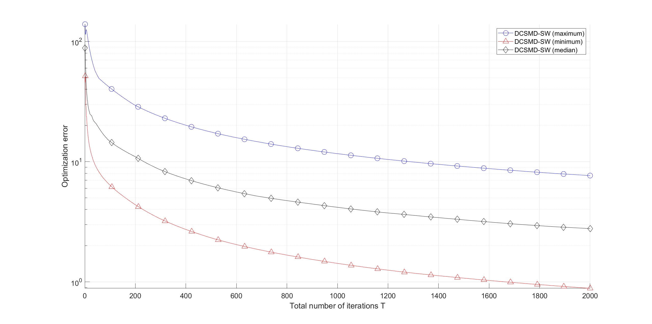
Figure 1: Maximum, minimum, and median of the optimization errors versus the total number of iterations $T$ of the DCSMD-SW algorithm.

In this section, we begin by performing numerical experiments to demonstrate various characteristics of the DCSMD-SW algorithm, with an emphasis on a distributed composite regularized linear regression problem:

$$\min_{x\in\mathcal{X}}\sum_{i=1}^{m}\left(\frac{1}{2}\left(\langle{a}_{i},{x}\rangle-b_{i}\right)^{2}+\lambda\|x\|_{1}\right)$$ (30)

where $a_{i}\in\mathbb{R}^{n}$ and $b_{i}\in\mathbb{R}$ are data known only to agent $i$. Unless stated otherwise, we will adopt the following configurations in our simulation examples. The constraint set is defined as $\mathcal{X}=\{x\in\mathbb{R}^{n}:u_{j}\leq[x]_{j}\leq v_{j},j=1,2,...,n\}$. The parameters and distance functions in DCSMD-SW are chosen as follows: we consider the number of agents $m=60$, the problem dimension $n=20$, the hyperparameter $\lambda=0.1$. The distance generating function is selected as $\Phi(x)=\frac{1}{2}\|x\|_{2}^{2}$ with $x\in\mathcal{X}$. The parameters for the constraints are $u_{j}=-1$ and $v_{j}=1$ for $j=1,2,..,n$. In each trial, for $i=1,2,...,m$, each element of the input vector $a_{i}$ is generated from a uniform distribution over the interval $[-1,1]$, and the response is generated by $b_{i}=\langle a_{i},x_{*}\rangle+\epsilon$, where $[x_{*}]_{i}=1$ for $1\leq i\leq\lfloor n/2\rfloor$ and $0$ otherwise, and the noise $\epsilon$ is drawn i.i.d. from a normal distribution $\mathcal{N}(0,1)$. The stochastic noise $\xi_{i,t}$ in the gradient is generated from a Gaussian distribution $\mathcal{N}(\mathbf{0},10^{-3}I_{n})$, which ensures that $\|\xi_{i,t}\|_{*}$ is a sub-Weibull random variable. The initial values $\{x_{i,1}\}_{i=1}^{m}$ are sampled from a uniform distribution on $[0,1]^{n}$. The stepsizes $\{\alpha_{k}\}$ are selected as $\alpha_{k}=\frac{1}{\sqrt{k+1}}$, $k\geq 0$. In our experiments, we evaluate the optimization error $F(\widetilde{x}_{\ell}^{T})-F(x^{*})$ ($\ell\in\mathcal{V}$), where $\widetilde{x}_{\ell}^{T}=\frac{1}{T}\sum_{t=1}^{T}x_{\ell,t}$ is the local ergodic sequence with equi-weight. All the experiment results are based on the average of 10 runs.

We demonstrate the convergence behavior of the DCSMD-SW algorithm by graphing the maximum, minimum, and median of the optimization errors $\{F(\widetilde{x}_{\ell}^{T})-F(x^{*})\}_{\ell=1}^{m}$ across $m$ agents, plotted against the total number of iterations $T$. The outcomes are presented in Fig. 1, which shows that all agents in the DCSMD-SW algorithm converge at a satisfactory rate.

Figure 2: Median of the optimization errors versus the total number of iterations $T$ of the DCSMD-SW algorithm for three different stochastic noises: uniform noise, Gaussian noise, and Laplace noise.

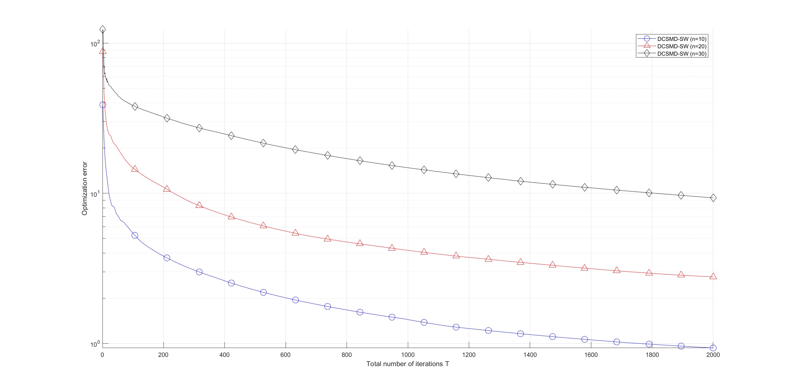
Figure 3: Median of the optimization errors versus the total number of iterations $T$ of the DCSMD-SW algorithm for three different choices of the problem dimension $n$.

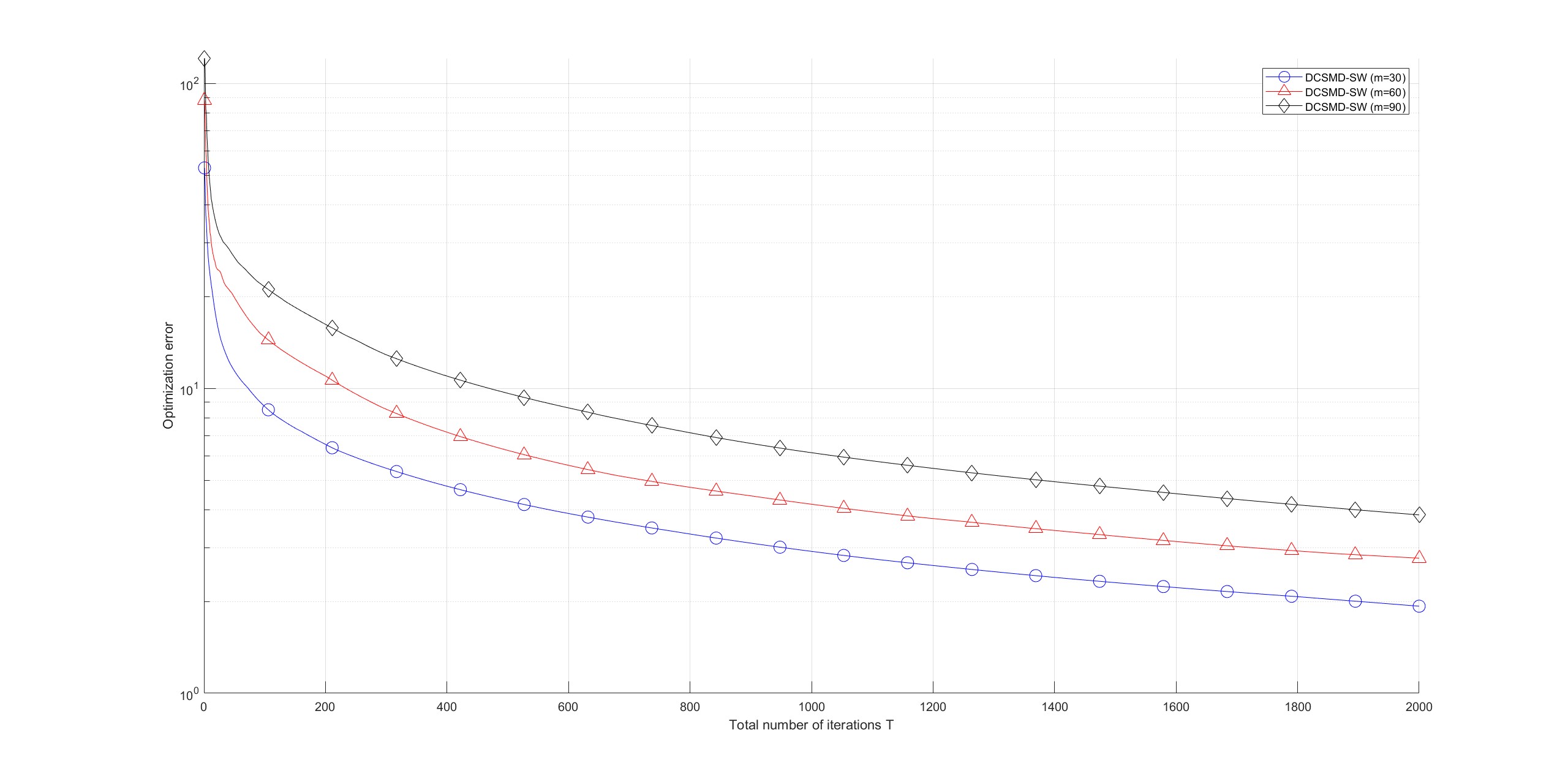
Figure 4: Median of the optimization errors versus the total number of iterations $T$ of the DCSMD-SW algorithm for three different number of agents $m$ in a ring network.

We begin by investigating the effect of various sub-Weibull stochastic noises $\xi_{i,t}$ on the convergence of the DCSMD-SW algorithm. Specifically, we analyze three distinct types of stochastic noise whose norm meet the sub-Weibull ($\theta$,$\kappa$) condition: uniform noise within the interval $[-0.5,0.5]^{n}$, Gaussian noise described by $\mathcal{N}(\mathbf{0},10^{-1}I_{n})$, and noise elements that follow a Laplace distribution $Laplace(0,10^{-1})$. These three scenarios adhere to the sub-Weibull conditions with increasing values of $\theta$. The simulation results illustrated in Fig. 2 align with our theoretical findings, indicating that the convergence rate of the DCSMD-SW algorithm slightly deteriorates as the tail parameter $\theta$ increases.

Next, we evaluate how the problem dimension $n$ influences the convergence of the DCSMD-SW algorithm. We select three different dimensions: $n=10$, $n=20$, and $n=30$, and plot the median of the optimization errors across all agents against the total number of iterations $T$. The results shown in Fig. 3 clearly demonstrate that DCSMD-SW exhibits improved optimality with smaller problem dimensions $n$.

Additionally, we analyze the impact of network size (number of agents $m$) on the convergence of the DCSMD-SW algorithm. We consider three different numbers of agents in a ring network: $m=30$, $m=60$, and $m=90$, and present the plots of the median of the optimization errors across all agents versus the total number of iterations $T$. The findings shown in Fig. 4 suggest that the DCSMD-SW algorithm performs more effectively with a smaller network size.

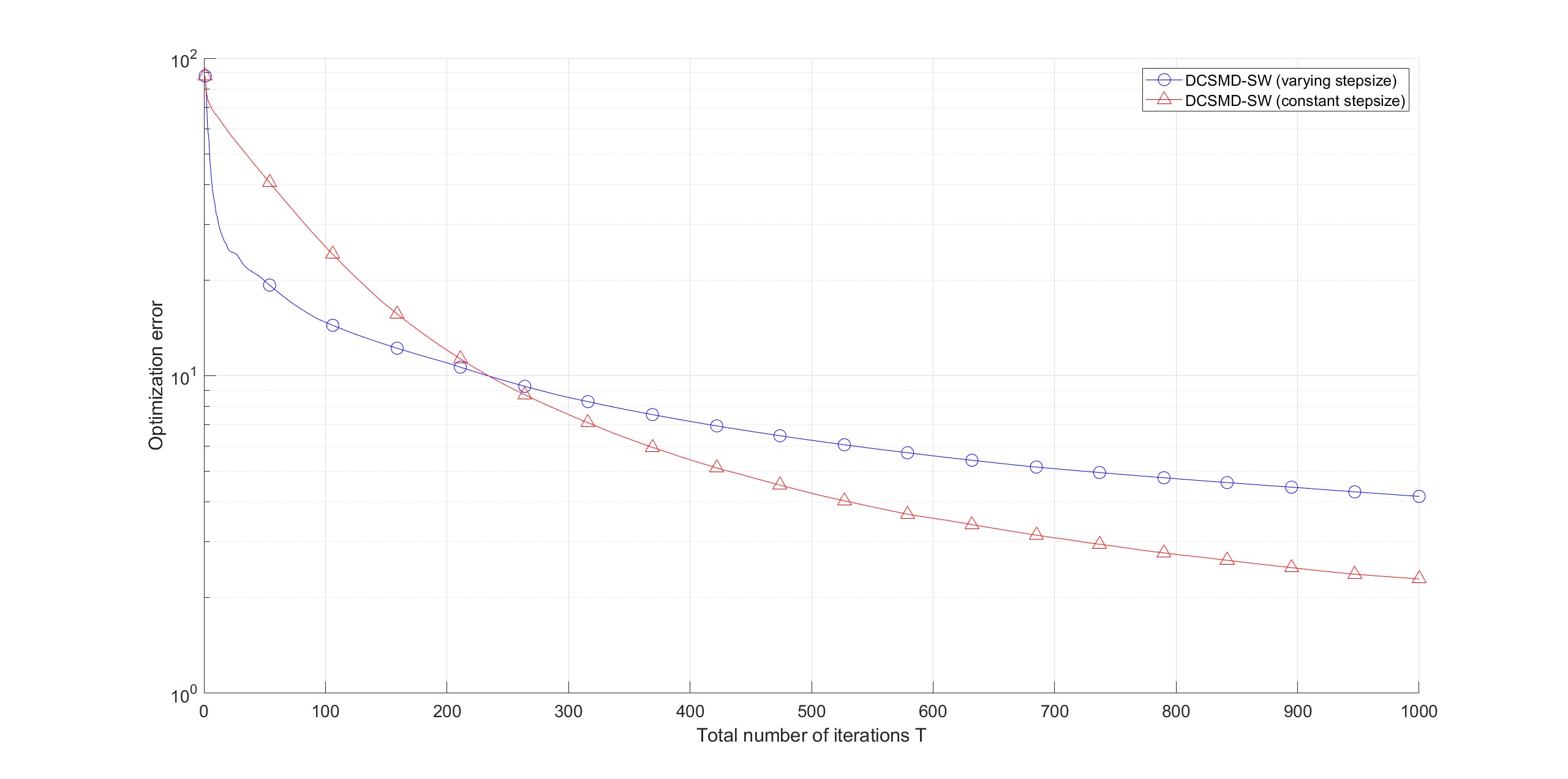
Figure 5: Median of the optimization errors versus the total number of iterations $T$ of the DCSMD-SW algorithm for two different stepsizes: constant stepsize and varying stepsize.

Subsequently, we explore the selection of a constant stepsize in relation to the time-horizon $T$, specifically $\alpha_{t}=\mathcal{O}(1/\sqrt{T})$. We illustrate the convergence of the DCSMD-SW algorithm using this constant stepsize and contrast it with a varying stepsize $\alpha_{t}=1/\sqrt{t+1}$ in Fig. 5. The results indicate that a well-chosen constant stepsize relative to the time-horizon can lead to a slightly faster convergence rate compared to the varying stepsize approach. This aligns with our theoretical conclusions, which suggest that the $(\log T)^{2}$ order can be eliminated when employing a constant strategy for stepsize selection if the time-horizon $T$ is known.

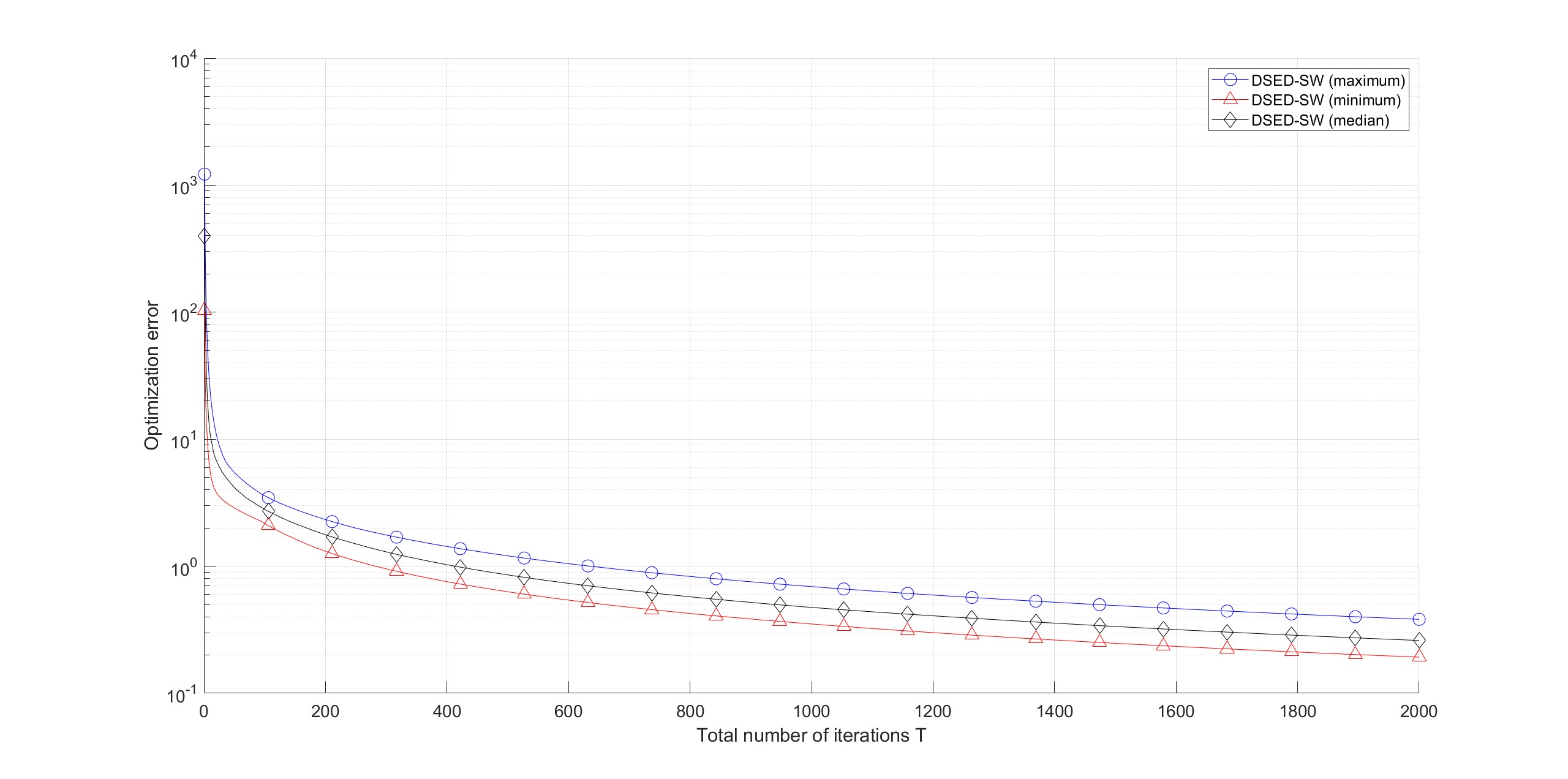
Figure 6: Maximum, minimum, and median of the optimization errors versus the total number of iterations $T$ of the DSED-SW algorithm.

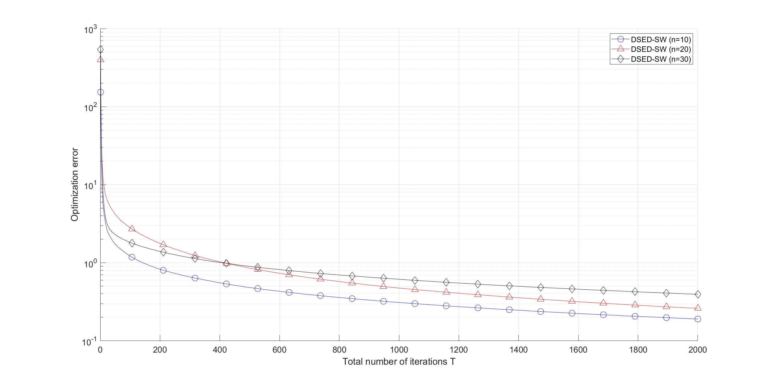
Figure 7: Median of the optimization errors versus the total number of iterations $T$ of the DSED-SW algorithm for three different choices of the problem dimension $n$.

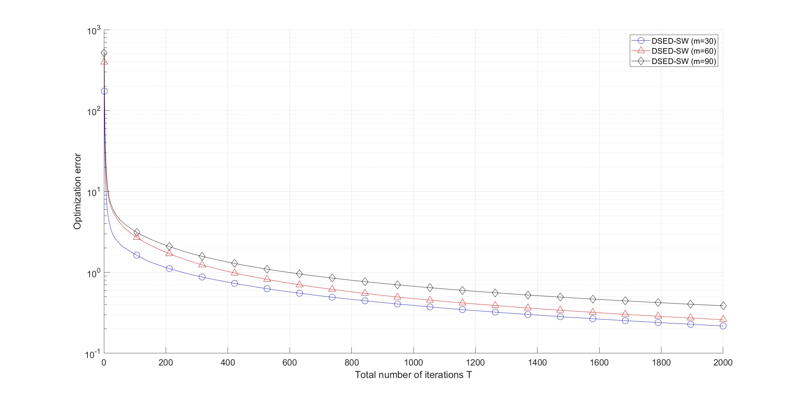
Figure 8: Median of the optimization errors versus the total number of iterations $T$ of the DSED-SW algorithm for three different number of agents $m$ in a ring network.

Finally, it is important to note that DSMD can offer adaptive updates that effectively account for the geometry of the underlying constraint set. Therefore, we focus on the specific DSED-SW algorithm, which addresses a distributed linear regression problem defined as follows: $\min_{x\in\mathcal{X}}\sum_{i=1}^{m}\frac{1}{2}\left(\langle{a}_{i},{x}\rangle-b_{i}\right)^{2}$, where we consider the probability simplex decision space $\mathcal{X}=\Delta_{n}=\{x\in\mathbb{R}^{n}:\sum_{i=1}^{n}[x]_{i}=1,[x]_{i}\geq 0,i\in[n]\}$, and utilize the Kullback-Leibler divergence $D_{\Phi}(x\|y)=\sum_{i=1}^{n}[x]_{i}\ln\frac{[x]_{i}}{[y]_{i}}$ induced by the Gibbs entropy function $\Phi(x)=\sum_{i=1}^{n}[x]_{i}\ln[x]_{i}$. The data is generated as previously described, other than that we choose $[x_{*}]_{i}=2/n$ for $1\leq i\leq n/2$ ($n$ is even) and $0$ otherwise. The initial values $\{x_{i,1}\}_{i=1}^{m}$ are drawn from a symmetric Dirichlet distribution with $\alpha=1$, which corresponds to a uniform distribution over the simplex $\Delta_{n}$.

We begin by illustrating the convergence performance of the DSED-SW algorithm through a plot of the maximum, minimum, and median optimization errors across all agents against the total number of iterations $T$. The outcomes, depicted in Fig. 6, indicate that the DSED-SW algorithm achieves a satisfactory convergence rate. Additionally, we evaluate the influence of the problem dimension $n$ and the number of agents $m$ on the convergence of the DSED-SW algorithm in Fig. 7 and Fig. 8, respectively. These results reveal that the DSED-SW algorithm performs better when either the problem dimension $n$ or the number of agents $m$ is reduced.

8 Conclusions and discussions

In this work, the distributed composite optimization problem in the context of sub-Weibull stochastic gradient noises is investigated. The convergence theory of DCSMD-SW is comprehensively established. The explicit convergence rate is fully derived for two types of ergodic approximating sequences generated from DCSMD-SW under appropriate selection rules of stepsizes. As a byproduct of this work, the convergence behaviors of two important distributed stochastic algorithms, DSGD and DSED, under the influence of sub-Weibull randomness have been directly obtained. Notably, the convergence characteristics of these two algorithms under sub-Weibull environment have not been independently studied in existing literature. Moreover, this work eliminates the need for the crucial technical assumption of boundedness of the decision set, which has been a dependency in existing research on DMD and DSMD approach for convex optimization. Finally, numerical experiments are conducted to support the theory in this work. It would be interesting to extend our analysis to other popular occasions such as distributed Nash equilibrium seeking, distributed strongly convex optimization and distributed online optimization. We leave them for our future work.

References

- [1] A. Nedić, A. Ozdaglar, “Distributed subgradient methods for multi-agent optimization.” IEEE Transactions on Automatic Control, 54(1), 48-61, 2009.
- [2] T. Yang, X. Yi, J. Wu, Y. Yuan, D. Wu, Z. Meng, Y. Hong, H. Wang, Z. Lin, K. H. Johansson. “A survey of distributed optimization.” Annual Reviews in Control. 47, 278-305, 2019.
- [3] M. Chiang, P. Hande, T. Lan, C. Tan. “Power control in wireless cellular networks.” Foundations and Trends in Networking, 2(4), pp. 381-533, 2008.
- [4] U. A. Khan, W. U. Bajwa, A. Nedić, M. G.. Rabbat, A. H. Sayed. “Optimization for data-driven learning and control.” Proceedings of the IEEE, 108(11), 2020.
- [5] P. Yi, Y. Hong and F. Liu, “Initialization-free distributed algorithms for optimal resource allocation with feasibility constraints and its application to economic dispatch of power systems,” Automatica, vol. 74, pp. 259-269, 2016.
- [6] T. H. Chang, A. Nedić, A. Scaglione. “Distributed constrained optimization by consensus-based primal-dual perturbation method.” IEEE Transactions on Automatic Control, 59(6), 1524-1538, 2014.
- [7] J. C. Duchi, A. Agarwal, M. J. Wainwright. “Dual averaging for distributed optimization: convergence analysis and network scaling.” IEEE Transactions on Automatic Control, 57(3), 592-606, 2012.
- [8] A. Nedić, A. Olshevsky. “Distributed optimization over time-varying directed graphs.” IEEE Transactions on Automatic Control, 60(3), 601-615, 2015.
- [9] D. Yuan, Y. Hong, D. W. Ho, G. Jiang. “Optimal distributed stochastic mirror descent for strongly convex optimization.” Automatica, 90, 196-203, 2018.
- [10] X. Yi, X. Li, T. Yang, L. Xie, T. Chai, K. H. Johansson. “Distributed bandit online convex optimization with time-varying coupled inequality constraints.” IEEE Transactions on Automatic Control, 66(10), 4620-4635, 2020.
- [11] S. Sundhar Ram, A. Nedić, V. V. Veeravalli. Distributed stochastic subgradient projection algorithms for convex optimization. Journal of Optimization Theory and Applications, 147, 516-545, 2010.
- [12] D. Yuan, Y. Hong, D. W. C. Ho, S. Xu. “Distributed mirror descent for online composite optimization.” IEEE Transactions on Automatic Control, 66(2), 714-729, 2021.
- [13] Z. Yu, D. W. Ho, D. Yuan. “Distributed randomized gradient-free mirror descent algorithm for constrained optimization.” IEEE Transactions on Automatic Control, 67(2), 957 - 964, Feb 2022.
- [14] J. Li, G. Li, Z. Wu, C. Wu. “Stochastic mirror descent method for distributed multi-agent optimization.” Optimization Letters, 12, pp. 1179-1197, 2018.
- [15] J. Li, G. Chen, Z. Dong, Z. Wu. “Distributed mirror descent method for multi-agent optimization with delay.” Neurocomputing, 177, 643-650, 2016.
- [16] J. Liu, Z. Yu, D. W. Ho. “Distributed constrained optimization with delayed subgradient information over time-varying network under adaptive quantization.” IEEE Transactions on Neural Networks and Learning Systems, 35(1), 143-156, 2022.
- [17] M. Xiong, B. Zhang, D. W. C. Ho, D. Yuan, S. Xu. “Event-triggered distributed stochastic mirror descent for convex optimization.” IEEE Transactions on Neural Networks and Learning Systems, 34(9), 6480-6491, 2022.
- [18] X. Fang, B. Zhang, D. Yuan. “Gossip-based distributed stochastic mirror descent for constrained optimization.” Neural Networks, 175, 106291, 2024.
- [19] G. Chen, G. Xu, W. Li, Y. Hong. “Distributed mirror descent algorithm with Bregman damping for nonsmooth constrained optimization.” IEEE Transactions on Automatic Control, 68(11), 6921-6928, 2023.
- [20] Y. Qin, K. Lu, H. Xu, X. Chen. “High probability convergence of clipped distributed dual averaging with heavy-tailed noises.” IEEE Transactions on Systems, Man, and Cybernetics: Systems, 2025.
- [21] C. Sun, B Chen. “Distributed stochastic strongly convex optimization under heavy-tailed noises.” In 2024 IEEE International Conference on Cybernetics and Intelligent Systems (CIS) and IEEE International Conference on Robotics, Automation and Mechatronics (RAM) (pp. 150-155). IEEE.
- [22] J. Li, C. Li, J. Fan, T. Huang. “Online distributed stochastic gradient algorithm for nonconvex optimization with compressed communication.” IEEE Transactions on Automatic Control, 69(2), 936-951, 2023.
- [23] U. Simsekli, L. Sagun, M. Gurbuzbalaban. “A tail-index analysis of stochastic gradient noise in deep neural networks.” International Conference on Machine Learning, pp. 5827-5837, 2019.
- [24] J. Zhang, S. P. Karimireddy, A. Veit, S. Kim, S. Reddi, S. Kumar, S. Sra. “Why are adaptive methods good for attention models?” Advances in Neural Information Processing Systems, 33, pp. 15383-15393, 2020.
- [25] Y. Lou, G. Shi, K. H. Johansson, Y. Hong. “Approximate projected consensus for convex intersection computation: Convergence analysis and critical error angle.” IEEE Transactions on Automatic Control, 59(7), 1722-1736, 2014.
- [26] K. Lu, H. Wang, H. Zhang, L. Wang. “Convergence in high probability of distributed stochastic gradient descent algorithms.” IEEE Transactions on Automatic Control, 69(4), 2189-2204, 2023.
- [27] Z. Yu, J. Fan, Z. Shi, D. X. Zhou. “Distributed gradient descent for functional learning.” IEEE Transactions on Information Theory, 70(9), 6547 - 6571, 2024.
- [28] X. Guo, T. Hu, Q. Wu. “Distributed minimum error entropy algorithms.” Journal of Machine Learning Research, 21(126), 1-31, 2020.
- [29] Z. C. Guo, T. Hu, L. Shi. “Gradient descent for robust kernel-based regression.” Inverse Problems, 34(6), 065009, 2018.
- [30] C. Sun, B. Chen, J. Wang, Z Wang, L. Yu. “Distributed stochastic Nash equilibrium seeking under heavy-tailed noises.” Automatica, 173, 112081, 2025.
- [31] N. Bastianello, L. Madden, R. Carli E. Dall’Anese. “A stochastic operator framework for optimization and learning with sub-weibull errors.” IEEE Transactions on Automatic Control, 2024.
- [32] L. Madden, E. Dall’Anese, S. Becker. “High probability convergence bounds for non-convex stochastic gradient descent with sub-weibull noise.” Journal of Machine Learning Research, 25(241), pp. 1-36, 2024.
- [33] K. Eldowa, A. Paudice. “General tail bounds for non-smooth stochastic mirror descent.” International Conference on Artificial Intelligence and Statistics, pp. 3205-3213. PMLR, 2024.
- [34] S. Li, Y. Liu. “High probability guarantees for nonconvex stochastic gradient descent with heavy tails.” International Conference on Machine Learning, pp. 12931-12963. PMLR, 2022.
- [35] M. Vladimirova, S. Girard, H. Nguyen, J. Arbel. “Sub-Weibull distributions: Generalizing sub-Gaussian and sub-Exponential properties to heavier tailed distributions.” Stat, 9(1), 2020.
- [36] F. Götze, H. Sambale, A. Sinulis. “Concentration inequalities for polynomials in -sub-exponential random variables.”Electronic Journal of Probability, 26. 2021.
- [37] T. Hu, X. Liu, K. Ji, Y. Lei. “Convergence of Adaptive Stochastic Mirror Descent.” IEEE Transactions on Neural Networks and Learning Systems, DOI: 10.1109/TNNLS.2025.3545420, early access, 2025.
- [38] Y. Lei, D. X. Zhou. “Convergence of online mirror descent.” Applied and Computational Harmonic Analysis, 48(1), 343-373, 2020.
- [39] M. Ye, G. Hu, F. L. Lewis. “Nash equilibrium seeking for -coalition noncooperative games.” Automatica, 95, 266-272, 2018.
- [40] Z. Feng, W. Xu, J. Cao. “Distributed Nash equilibrium computation under round-robin scheduling protocol.” IEEE Transactions on Automatic Control, 69(1), 339-346, 2023.