A Geometric Multigrid Preconditioner for Discontinuous Galerkin Shifted Boundary Method

Abstract

This paper introduces a geometric multigrid preconditioner for the Shifted Boundary Method (SBM) designed to solve PDEs on complex geometries. While SBM simplifies mesh generation by using a non-conforming background grid, it often results in non-symmetric and potentially ill-conditioned linear systems that are challenging to solve efficiently. Standard multigrid methods with pointwise smoothers prove ineffective for such systems due to the localized perturbations introduced by the shifted boundary conditions. To address this challenge, we introduce a Discontinuous Galerkin (DG) formulation for SBM that enables the design of a cell-wise multiplicative smoother within an $hp$-multigrid framework. The element-local nature of DG methods naturally facilitates cell-wise correction, which can effectively handle the local complexities arising from the boundary treatment. Numerical results for the Poisson equation demonstrate favorable performance with mesh refinement for linear ($p=1$) and quadratic ($p=2$) elements in both 2D and 3D, with iteration counts showing mild growth. However, challenges emerge for cubic ($p=3$) elements, particularly in 3D, where the current smoother shows reduced effectiveness.

1 Introduction

Solving partial differential equations on domains with complex or evolving geometries presents a significant challenge. Traditional numerical methods, such as the finite element method (FEM), often require body-fitted meshes, which can be difficult to generate for intricate shapes. Unfitted finite element methods offer an attractive alternative by employing a fixed background mesh that does not conform to the physical domain boundary. Among these, the Shifted Boundary Method (SBM) [33] stands out by defining the problem on a surrogate domain composed of cells from the background mesh and extrapolating boundary conditions from the true boundary to the boundary of these selected cells. This approach avoids complex cell-cutting procedures and specialized quadrature rules common in methods like CutFEM [18]. However, this geometric simplicity often results in ill-conditioned linear systems that are challenging to solve efficiently.

Despite its advantages, the development of robust and scalable solvers for SBM, particularly geometric multigrid preconditioners [28], has remained an open problem. This paper addresses this gap by introducing a geometric multigrid preconditioner specifically designed for SBM. To enable effective smoothing within the multigrid procedure, in particular to address the non-symmetric and potentially indefinite local structure of cell matrices adjacent to the surrogate boundary, we introduce the Discontinuous Galerkin (DG) method [45] for SBM discretizations, which, to the best of author’s knowledge, has also not been previously investigated. This allows us to leverage the inherent discontinuity of the DG method to design a cell-wise smoother that effectively addresses the local perturbations introduced by the SBM discretization. Consequently, the design of a geometric multigrid solver tailored for discontinuous Galerkin SBM discretizations is the primary contribution of this work.

In SBM, the surrogate domain $\tilde{\Omega}$ is typically constructed as a union of cells from a fixed background mesh that are deemed active (e.g., entirely inside or significantly intersecting the true domain $\Omega$), and its boundary $\tilde{\Gamma}$ does not conform to the domain boundary $\Gamma$. Boundary conditions are transferred from the true to the surrogate boundary, typically via Taylor expansions or more general extension operators [46], and enforced in a Nitsche-like manner [35]. The Shifted Boundary Method has evolved from its first formulation [33, 34], which used cells strictly within the considered domain, to a recent approach [44] that often include intersected cells based on a volume fraction threshold. It has been extended to high-order discretizations [9], various physical problems including Stokes flow [5], solid mechanics [8, 10], and significantly, to problems with embedded interfaces [32, 41]. These latter works demonstrate the capability of SBM to handle discontinuities across internal boundaries by appropriately modifying the formulation to impose jump conditions, extending the method’s applicability to multiphysics and multi-material problems. Other innovations include penalty-free variants [23] and integration with level set methods [31, 43].

While this avoids the complexities of generating body-fitted meshes, the primary geometric task in SBM shifts to accurately determining the relationship between points on the surrogate boundary $\tilde{\Gamma}$ and the true boundary $\Gamma$. The method inherently allows for the use of arbitrarily complex geometries, and crucially, avoids the need to compute integrals over the arbitrarily shaped integration domains that arise from cell-boundary intersections. However, for each point on $\tilde{\Gamma}$, one must find its closest point projection onto $\Gamma$, which is still a non-trivial problem, especially for complex or implicitly defined geometries. Level set methods, which represent the domain boundary as the zero level set of a function, are often employed in unfitted methods like SBM to facilitate operations such as closest point projection [31, 43]. Special treatment of domains with corners was analyzed in [7].

However, the geometric flexibility of SBM comes at the cost of new computational challenges. The extrapolation of boundary conditions and the resulting modifications to the variational formulation often lead to linear systems with non-symmetric and potentially indefinite properties, particularly for higher-order polynomial approximations, making their efficient solution non-trivial.

Multigrid methods [16, 28] are renowned for their potential to solve large systems arising from partial differential equations, often offering optimal or near-optimal complexity. However, their application as preconditioners for SBM remains largely unexplored. While Algebraic Multigrid (AMG) has been applied to SBM for discretizations using continuous linear elements [6], its efficiency for higher-order methods is not established, and AMG may not fully leverage the geometric information in structured background meshes. Geometric multigrid methods, in contrast, explicitly use the hierarchy of meshes and can be very effective, especially when combined with structured or semi-structured background grids often employed in SBM. A critical component of geometric multigrid is the smoother, which damps high-frequency error components on each grid level. Standard smoothers like Jacobi or Gauss-Seidel, however, may struggle with the non-standard local properties of SBM systems occurring at the surrogate boundary. This motivates the exploration of alternative discretization and smoothing strategies.

The non-symmetric and potentially indefinite nature of the local matrices arising from SBM presents challenges for standard multigrid smoothers. To address this, we turn to discontinuous Galerkin methods, whose element-local structure naturally facilitates the construction of cell-wise smoothers that can effectively manage the local complexities introduced by SBM.

Discontinuous Galerkin methods [37, 45, 4, 22] employ piecewise discontinuous polynomials as basis functions. In interior penalty formulations [11, 4], continuity is enforced weakly by penalizing jumps across element interfaces. Alternatively, non-symmetric variants exist [13, 36], which generally exhibit reduced accuracy compared to symmetric formulations [45]. While DG methods typically involve a higher number of degrees of freedom compared to their continuous Galerkin counterparts, they offer considerable flexibility in return, especially for implementing Schwarz-like smoothers or $hp$-adaptivity.

The synergy between multigrid techniques and DG discretizations has been a fruitful area of research, leading to powerful solvers. The inherent block structure of DG methods lends itself naturally to the design of effective smoothers, a cornerstone of multigrid efficiency. Seminal work, such as the overview in [2], has established $hp$-independent convergence rates, a highly desirable property, though the number of smoothing iterations can sometimes scale with the polynomial degree $p$. Particularly for DG discretizations on structured Cartesian meshes, specialized smoothers like cell-wise or vertex-patch variants have proven highly effective. When dealing with separable operators like the Laplacian, the local problems arising in these smoothers can often be solved with impressive efficiency via fast diagonalization techniques [40, 39]. This can translate into low iteration counts and robust $hp$-independent convergence. Furthermore, the adaptability of DG methods to modern hardware architectures is underscored by successful GPU implementations of multilevel solvers, showcasing their potential for high-performance computing [24].

The cell-wise and vertex-patch smoothers, mentioned earlier as effective for DG discretizations, can be formally understood and analyzed within the framework of subspace correction methods. This perspective is particularly valuable for designing smoothers capable of addressing the local complexities introduced by SBM, such as the non-standard boundary conditions that can conflict with traditional smoothers. The theory of subspace correction methods [42, 15] provides a powerful framework for analyzing and constructing such smoothers. While we do not provide a theoretical analysis of the convergence of our multigrid preconditioner, we use insights from subspace correction theory to guide the design of our smoother. We adopt this perspective and design our cell-wise smoother as a successive subspace correction method, where each subspace corresponds to the degrees of freedom on a single cell. The key aspect of this design is the choice of subspace, which allows for effective accounting for the shifted boundary condition. For practical efficiency, especially with high-order DG methods, the implementation of these smoothers and the overall multigrid algorithm can significantly benefit from matrix-free techniques.

Matrix-free implementations significantly enhance the efficiency of DG methods, especially for high-order discretizations and large problems [30, 40]. Geometric multigrid methods are particularly well-suited for matrix-free settings, as their components can often be implemented efficiently without explicit matrix formation [30]. While this work uses matrix-based implementations to demonstrate the multigrid approach for DG-SBM, it lays the groundwork for future matrix-free solvers.

In the broader context of unfitted methods, CutFEM [18] is a prominent alternative with theoretical results for preconditioners already developed. It discretizes directly on the physical domain by cutting background cells, requiring specialized quadrature for handling these intersected cells. Due to inherent difficulties with small cuts, proper stabilization seems to be an unavoidable part of CutFEM. The so-called ghost penalty [17, 39] solves the issue of ill-conditioning but may require additional care to avoid locking [12, 14, 20]. CutFEM has been applied to various problems, including Stokes [19], elasticity [29], or two-phase flows [21]. Furthermore, Discontinuous Galerkin methods have also been combined with CutFEM [27, 14].

Concerning the preconditioning, CutFEM seems to pose challenges. Results providing optimal preconditioners [26, 25] have been developed. Although these methods are shown to be mesh-independent, iteration counts can be high. In [14] DG-CutFEM was considered, and a multigrid preconditioner based on cell-wise Additive Schwarz smoother was used. Although the paper mostly focuses on matrix-free implementation, the preconditioner seems promising. However, the smoothing step requires a rather high number of matrix-vector products.

This paper addresses the computational challenges of solving linear systems arising from SBM discretizations. Our main contribution is a geometric multigrid preconditioner specifically designed for Discontinuous Galerkin SBM formulations of the Poisson equation. We develop a cell-wise successive subspace correction smoother that aligns with the DG framework and the localized nature of SBM. Numerical experiments demonstrate the preconditioner’s effectiveness under mesh refinement, showing strong performance for linear ($p=1$) and quadratic ($p=2$) elements, while identifying challenges for cubic ($p=3$) elements, particularly in 3D. The implementation is built on the deal.II finite element library [3, 1], which provides comprehensive tools for finite element methods and multigrid. The closest point search was implemented specifically for this work.

The remainder of this paper is organized as follows. Section 2 details the SBM formulation and its DG discretization. Section 3 describes the components of the multigrid preconditioner, with a focus on the smoother design. Section 4 discusses implementation aspects, including geometry handling and the closest point projection algorithm. Numerical results evaluating the performance of the proposed method are presented in Section 5. Finally, Section 6 offers concluding remarks and outlines potential directions for future research.

2 Method formulation

We consider the Poisson problem as a model problem:

$$-\Delta u =f\quad\text{in }\Omega,$$ (1)

$$u =g\quad\text{on }\Gamma,$$ (2)

where $\Omega\subset\mathbb{R}^{d}$ ($d=2,3$) is a domain with boundary $\Gamma=\partial\Omega$ as depicted in Figure 1, $f$ is a given source term, and $g$ is the prescribed Dirichlet boundary condition.

To solve this problem numerically, we first formulate it in a weak sense. We seek a solution $u$ in an appropriate function space, $H^{1}(\Omega)$, which consists of functions that are square-integrable and whose first derivatives are also square-integrable. Multiplying the equation by a test function $v\in H^{1}(\Omega)$ and integrating over $\Omega$, we obtain:

$$\int_{\Omega}\nabla u\cdot\nabla v\,dx-\int_{\Gamma}(\nabla u\cdot\mathbf{n})\,v\,ds=\int_{\Omega}f\,v\,dx.$$

We next introduce a triangulation $\mathcal{T}_{h}$ consisting of quadrilateral (2D) or hexahedral (3D) elements of size $h$, and define a finite element space $\mathbb{V}_{h}\subset H^{1}(\Omega)$ using Lagrange polynomial elements of degree $p$. In classical finite element methods, the mesh conforms to the boundary (unlike the background mesh approach illustrated in Figure 1), and test functions $v$ typically vanish on $\Gamma$ to strongly enforce the Dirichlet condition $u=g$. When function spaces do not necessarily satisfy essential boundary conditions strongly, boundary conditions must be enforced weakly through additional integral terms on $\Gamma$.

Nitsche’s method provides a way to weakly impose Dirichlet boundary conditions within a variational formulation without requiring the function space to satisfy the boundary conditions. It modifies the bilinear form by adding terms on the boundary $\Gamma$. The standard Nitsche formulation for the Poisson problem with Dirichlet boundary conditions $u=g$ on $\Gamma$ seeks $u_{h}\in V_{h}$ such that for all $v_{h}\in\mathbb{V}_{h}$:

$$\begin{split}\int_{\Omega}\nabla u_{h}\cdot\nabla v_{h}\,dx\;\;-\int_{\Gamma}(\nabla u_{h}\cdot\mathbf{n})v_{h}\,ds-&\alpha\int_{\Gamma}(\nabla v_{h}\cdot\mathbf{n})u_{h}\,ds+\int_{\Gamma}\sigma u_{h}v_{h}\,ds=\\ &=\int_{\Omega}fv_{h}\,dx-\int_{\Gamma}(\nabla v_{h}\cdot\mathbf{n})g\,ds+\int_{\Gamma}\sigma_{\Gamma}gv_{h}\,ds.\end{split}$$

Here, $\sigma_{\Gamma}$ is a penalty parameter, typically chosen as $\sigma_{\Gamma}=\mathcal{O}(p^{2}h^{-1})$ for mesh size $h$, and $\mathbf{n}$ is the outward unit normal vector to $\Gamma$. The choice of parameter $\alpha=1$ leads to a symmetric formulation, while $\alpha=-1$ results in a non-symmetric formulation in which the penalty term can be skipped [13]

Figure 1: Schematic illustrating the background mesh, interior cells (green), the surrogate boundary $\tilde{\Gamma}$ (thick blue line) along the upper boundary of the interior cells, and the true boundary $\partial\Omega$ (red).

2.1 Shifted Boundary Method

In many applications, the domain $\Omega$ may have a complex geometry, making the generation of body-fitted meshes challenging. Non-body-fitted (unfitted) methods address this challenge by employing a background mesh $\mathcal{T}_{h}$ that does not conform to the boundary of $\Omega$. The domain $\Omega$ is embedded within this background mesh, and cells of $\mathcal{T}_{h}$ are classified as active based on their intersection with $\Omega$. The computational domain $\tilde{\Omega}$ is defined as the union of these active cells. In the original SBM formulation [33], only cells strictly contained in $\Omega$ were included, leading to the surrogate domain boundary depicted by the solid blue line in Figure 1. Consequently, the surrogate domain $\tilde{\Omega}$ is generally a subset of $\Omega$, and its boundary $\tilde{\Gamma}$ does not coincide with the true boundary $\Gamma$.

Later extensions include intersected cells [44] with a volume fraction inside $\Omega$ greater than a threshold $\lambda\in[0,1]$. In Figure 1, this corresponds to including additional cells as indicated by the dashed blue line. This approach reduces the distance between true and surrogate boundaries, but can lead to ill-conditioning.

To impose boundary conditions on $\tilde{\Gamma}$, the Dirichlet condition prescribed on the true boundary $\Gamma$ is extrapolated to the surrogate boundary. This is typically accomplished by projecting points from $\tilde{\Gamma}$ onto the true boundary $\Gamma$ along a suitable direction (e.g., the outward normal to $\tilde{\Gamma}$) and using a Taylor expansion to approximate the boundary values. This is accomplished via an extension operator $\mathcal{E}$, which maps functions defined on $\tilde{\Omega}$ to the surrogate boundary $\tilde{\Gamma}$.

We assume that the Dirichlet boundary condition $g$ is given as a restriction of a function $u^{\star}$ defined on the entire domain $\Omega$ to the boundary $\Gamma$. While the choice of this function $u^{\star}$ (as an extension of $g$ from $\Gamma$ into $\Omega$) is not unique, we take $u^{\star}$ to be equal to the solution $u$ in the surrogate domain $\tilde{\Omega}$. For each point $\tilde{\mathbf{x}}\in\tilde{\Gamma}$, let $\mathbf{x}\in\Gamma$ be its closest point projection onto the true boundary, and let $\mathbf{d}=\mathbf{x}-\tilde{\mathbf{x}}$ be the shift vector. The function $u$ is extended from $\Gamma$ to $\tilde{\Gamma}$ using a Taylor expansion:

$$\mathcal{E}u^{\star}(\tilde{\mathbf{x}})=u^{\star}(\mathbf{x})-\mathbf{d}\cdot\nabla u(\tilde{\mathbf{x}})+\cdots$$

where $\mathcal{E}u^{\star}$ denotes the extrapolated boundary condition. The function $u^{\star}$ is assumed to be smooth in a neighborhood of $\tilde{\Gamma}$, which allows for the Taylor expansion to be valid. By substituting it into the weak formulation, we obtain a variational formulation for the shifted boundary problem with the extrapolated boundary condition on $\tilde{\Gamma}$ enforced in a Nitsche-like manner.

The SBM weak formulation seeks $u_{h}\in V_{h}$ such that for all $v_{h}\in V_{h}$,

$$\begin{split}\int_{\tilde{\Omega}}\nabla u_{h}\cdot\nabla v_{h}\,dx-\int_{\tilde{\Gamma}}(\nabla u_{h}\cdot\tilde{\mathbf{n}})v_{h}\,ds-\alpha\int_{\tilde{\Gamma}}(\nabla v_{h}\cdot\tilde{\mathbf{n}})\;\mathcal{E}u_{h}\,ds+\int_{\tilde{\Gamma}}\sigma_{\Gamma}\;\mathcal{E}u_{h}\;v_{h}\,ds=\\ =\int_{\tilde{\Omega}}fv_{h}\,dx-\int_{\tilde{\Gamma}}(\nabla v_{h}\cdot\tilde{\mathbf{n}})g^{E}\,ds+\int_{\tilde{\Gamma}}\sigma_{\Gamma}gv_{h}\,ds.\end{split}$$

where $\tilde{\mathbf{n}}$ is the outward normal to $\tilde{\Gamma}$ and $\sigma_{\Gamma}$ is a penalty parameter. We notice that our discrete solution $u_{h}$ is a piecewise polynomial function defined on the background mesh $\mathcal{T}_{h}$, hence its Taylor expansion can be computed directly by evaluating the function values at the points on the true boundary $\Gamma$. This allows us to avoid computation of higher-order derivatives of $u_{h}$. Note that the resulting form is no longer symmetric due to the presence of the extrapolated boundary condition. We will refer to formulation with $\alpha=1$ as the quasi-symmetric formulation.

Moreover, a simple 1D experiment using the domain $\Omega=[0,\xi]$ with a surrogate domain $\tilde{\Omega}=[0,1]$ and a single cell shows that for Lagrange polynomials of degree $p>1$, the stiffness matrix can have negative entries on the diagonal. As a result, the system matrix may lose diagonal dominance, which can adversely affect the stability and convergence of iterative solvers.

Notably, a penalty-free formulation ($\sigma_{\Gamma}=0$) can be achieved by setting $\alpha=-1$, which alters the sign of the extrapolated term in the weak formulation [23]. This approach also results in a positive diagonal for the stiffness matrix, and both formulations yield optimal convergence rates. However, symmetry of the remaining terms in the weak formulation is not recovered. Consequently, the 1D system matrix for this problem can exhibit complex eigenvalues when the true boundary $\xi$ is less than the surrogate boundary (i.e., $\xi<1$). Figure 2 illustrates this by plotting the maximum imaginary part of the eigenvalues for this 1D problem across different polynomial degrees $p$.

Figure 2 reveals that complex eigenvalues with non-zero imaginary parts indeed arise for negative shifts (when the true domain boundary $\xi$ is less than the surrogate domain boundary, $\xi<1$). The penalty-free formulation (dashed lines) exhibits eigenvalues with larger imaginary parts compared to the quasi-symmetric penalty formulation (solid lines) in this regime, while for positive shifts ($\xi>1$), the eigenvalues remain real for both formulations. The presence of complex eigenvalues is problematic for multigrid methods, as they can adversely affect smoothing properties and overall convergence of the preconditioner. Due to the tensor product structure of the Laplace operator, these 1D observations suggest that similar issues with complex eigenvalues may manifest in higher dimensions (2D and 3D), potentially compromising the effectiveness of standard smoothers and degrading multigrid performance.

Interestingly, for higher-order polynomials ($p>1$), the penalty-free formulation can yield eigenvalues with nonzero imaginary parts even when the surrogate boundary coincides with the true boundary ($\xi=1$). In contrast, the quasi-symmetric formulation is generally less prone to such imaginary eigenvalues. For this reason, we choose the quasi-symmetric formulation as the default in our work.

Figure 2: Maximal imaginary part of eigenvalues for the 1D SBM stiffness matrix versus true domain size $\xi$. The surrogate domain is $[0,1]$ (single cell); $\xi=1$ implies coincident boundaries. Solid lines: quasi-symmetric penalty ($\alpha=1$, $\sigma_{\Gamma}=5$); dashed lines: non-symmetric penalty ($\alpha=-1$, $\sigma_{\Gamma}=0$).

These observed spectral properties, particularly the emergence of complex eigenvalues, stem from the SBM’s treatment of boundary conditions on the surrogate boundary $\tilde{\Gamma}$. The effects of this treatment are localized to the cells adjacent to $\tilde{\Gamma}$ where the extrapolation and non-standard penalty terms are applied. Intuitively, one might expect that the Laplacian-like properties are perturbed only within these boundary-adjacent cells. This localization suggests that it should be possible to resolve these local perturbations within the scope of individual cells. Discontinuous Galerkin (DG) methods offer a natural framework for such a cell-wise treatment, as they inherently allow for different solution behaviors and formulations on each element and provide mechanisms to couple them appropriately.

2.2 Discontinuous Galerkin Discretization

We define the DG finite element space ${\mathbb{V}_{h}^{\text{DG}}}$ as piecewise polynomial functions of degree $p$ on the mesh $\mathcal{T}_{h}$, without continuity requirements across element boundaries. The DG weak formulation extends the standard variational formulation by incorporating terms that account for discontinuities across interior faces $\mathcal{F}_{h}^{\text{int}}$.

For a scalar function $w$, we define the jump operator $[w]$ and the average operator $\{w\}$ across an interior face $F\in\mathcal{F}_{h}^{\text{int}}$ as:

$$[w] =w^{+}\mathbf{n}^{+}+w^{-}\mathbf{n}^{-},$$

$$\{w\} =\frac{1}{2}(w^{+}+w^{-}),$$

where $w^{+}$ and $w^{-}$ denote the values of $w$ on the two elements sharing the face $F$, and $\mathbf{n}^{+}$ and $\mathbf{n}^{-}$ are the outward unit normal vectors to $F$ on these elements. In the symmetric interior penalty discontinuous Galerkin method, the bilinear form is modified to include these jump and average terms as follows:

$$\begin{split}\int_{\tilde{\Omega}}\nabla u_{h}\cdot\nabla v_{h}\,dx\longrightarrow\int_{\mathcal{T}_{h}}\nabla u_{h}\cdot\nabla v_{h}\,dx&-\sum_{F\in\mathcal{F}_{h}^{\text{int}}}\int_{F}\big{(}\{\nabla u_{h}\}\cdot[v_{h}]+\{\nabla v_{h}\}\cdot[u_{h}]\big{)}\,ds\\ &+\sum_{F\in\mathcal{F}_{h}^{\text{int}}}\int_{F}\sigma_{F}[u_{h}]\cdot[v_{h}]\,ds=a_{\tilde{\Omega}}(u_{h},v_{h}).\end{split}$$

The first term represents the standard DG contribution, while the second and third terms account for the discontinuities across the interior faces. The penalty term involving the parameter $\sigma_{F}$ ensures stability of the method.

By putting the form $a_{\tilde{\Omega}}(u_{h},v_{h})$ from the equation above together with the Nitsche-like term, we obtain the complete bilinear form for the DG-SBM discretization of the Poisson problem. The problem seeks $u_{h}\in{\mathbb{V}_{h}^{\text{DG}}}$ such that for all $v_{h}\in{\mathbb{V}_{h}^{\text{DG}}}$:

$$\begin{split}a_{h}(u_{h},v_{h})=a_{\tilde{\Omega}}(u_{h},v_{h})-\int_{\tilde{\Gamma}}(\nabla u_{h}\cdot\tilde{\mathbf{n}})v_{h}\,ds-&\alpha\int_{\tilde{\Gamma}}(\nabla v_{h}\cdot\tilde{\mathbf{n}})\mathcal{E}u_{h}\,ds+\int_{\tilde{\Gamma}}\sigma_{\Gamma}\mathcal{E}u_{h}v_{h}\,ds=\\ &=\int_{\tilde{\Omega}}fv_{h}\,dx-\int_{\tilde{\Gamma}}(\nabla v_{h}\cdot\tilde{\mathbf{n}})g\,ds+\int_{\tilde{\Gamma}}\sigma_{\Gamma}gv_{h}\,ds.\end{split}$$

By choosing a basis $\{\phi_{i}\}_{i=1}^{N}$ for ${\mathbb{V}_{h}^{\text{DG}}}$ in a standard form, we arrive at a linear system $Au_{h}=F$, where $A_{ij}=a_{h}(\phi_{i},\phi_{j})$, $u$ is the vector of coefficients. Since the basis defines a one-to-one mapping between real vectors and functions from ${\mathbb{V}_{h}^{\text{DG}}}$, we will not distinguish between these two.

3 Multigrid Preconditioner

The DG-SBM formulation described above leads to a large, sparse linear system. Due to the lack of symmetry and possible indefiniteness of the resulting matrix, we employ a Krylov subspace method, specifically GMRES, for its solution. The convergence of GMRES is sensitive to the condition number of the system matrix that grows with both the number of elements in the mesh and the polynomial degree. Multigrid methods [28] rely on a hierarchy of meshes with varying resolution levels. Our Cartesian background mesh naturally facilitates the construction of such a nested hierarchy. We define a sequence of meshes $\{\mathcal{T}_{\ell}\}_{\ell=0}^{L}$, where $\ell$ denotes the level and $L$ is the finest level. For each level, we identify active cells that have at least a fraction $\lambda$ of their measure (area in 2D, volume in 3D) inside the domain. On each mesh $\mathcal{T}_{\ell}$, we define a finite element space ${\mathbb{V}_{\ell}^{\text{DG}}}$ consisting of piecewise polynomials of  degree $p_{\ell}$. Since the set of active cells is determined by their intersection with the domain boundary, these sets are not necessarily nested between levels, which can affect the efficiency of standard inter-grid transfer operators. While our construction ensures a nested hierarchy of finite element spaces, the lack of a strict geometric relationship between active cells at different levels may reduce the effectiveness of transfer operators. We mitigate this potential efficiency loss by using only linear elements on geometrically coarser meshes and gradually increasing the polynomial degree only on the finest mesh. Hence the resulting total number of levels is $L+p$.

With this hierarchy of meshes and spaces established, the multigrid method is defined through two crucial components: the smoothers, which reduce high-frequency error components on each level, and the transfer operators, which move information between different resolution levels. These components, together with a coarse-grid solver, form the complete multigrid algorithm. For preconditioning, we use a single multigrid V-cycle.

3.1 Smoother

We first consider Richardson iterations with preconditioners $P$. Given the current approximation $u_{h}$ and the right-hand side $f_{h}$, a smoothing step updates the approximation:

$$u_{h}^{k+1}=u_{h}^{k}+P(f_{h}-A_{h}u_{h}^{k}).$$

We decompose the space ${\mathbb{V}_{\ell}^{\text{DG}}}$ into a sum of subspaces $\mathbb{V}_{i}$, i.e., ${\mathbb{V}_{\ell}^{\text{DG}}}=\sum_{i=1}^{N}\mathbb{V}_{i}$. Let $A_{i}$ be the restriction of $A$ to the subspace $\mathbb{V}_{i}$. Then, the additive subspace correction preconditioner is defined as:

$$P=\omega\sum_{i=1}^{N}A_{i}^{-1}$$

where $\omega$ is a relaxation parameter. Alternatively, the successive subspace correction method is a subspace correction method where the subspaces $\mathbb{V}_{i}$ are visited in a sequential manner. The procedure can be performed by applying one Richardson iteration with the preconditioner $P_{i}$ for each subspace $\mathbb{V}_{i}$. Since in each step only one subspace is corrected, the residual only changes locally and an efficient implementation is possible. The preconditioner updates the solution by sequentially applying corrections for each subspace. For each subspace $\mathbb{V}_{i}$, a correction is computed and applied:

$$u_{h}\leftarrow u_{h}+R_{i}^{T}A_{i}^{-1}R_{i}(f_{h}-A_{h}u_{h}).$$

This process is repeated for all subspaces $i=1,\ldots,N$. If the subspaces are chosen as one-dimensional spaces spanned by the basis functions, then the preconditioner is equivalent to either Jacobi (additive) or Gauss-Seidel (successive).

In the context of DG, a natural choice for the subspaces $\mathbb{V}_{i}$ is the set of functions that are non-zero only on a single cell. This leads to a cell-wise smoother, where we correct the solution on each cell independently. This can be interpreted as a block Gauss-Seidel smoother, where each block corresponds to the degrees of freedom associated with a single cell.

Viewing the smoother as a subspace correction method reveals important insights into the convergence properties. The correction computed within a subspace $\mathbb{V}_{i}$ implicitly satisfies certain boundary conditions on the boundary of that subspace. This is particularly important in the context of the SBM, where the boundary conditions are shifted. A careless choice of subspace can lead to overconstraining the correction, preventing certain error components from being effectively smoothed. For instance, Jacobi and Gauss-Seidel smoothers for continuous finite element methods, which correspond to vertex-patch smoothing with zero correction at patch boundaries, conflict with the shifted boundary conditions and are not effective, as confirmed in our preliminary numerical experiments. In contrast, the cell-wise smoother aligns well with the DG method’s element-based structure and takes into account the local nature of the SBM boundary conditions, correcting the solution on each cell independently, as illustrated in Figure 3.

We adopt this perspective and design our cell-wise smoother as a successive subspace correction method. Specifically, we implement a cell-wise Symmetric Successive Over-Relaxation (SSOR) smoother, which is a variant of the block Gauss-Seidel method where each block corresponds to the degrees of freedom on a single cell.

Figure 3: Illustration of a cell $K$ within the DG-SBM framework, highlighting different face types relevant to the cell-wise smoother. Interior faces ($\mathcal{F}_{h}^{\text{int}}$, green) connect to neighboring active cells. For cells adjacent to the domain boundary, faces can be part of the surrogate boundary $\tilde{\Gamma}$ (blue), which is shifted from the true boundary $\Gamma$ (red). The cell-wise smoother solves a local problem on $K$, implicitly handling these conditions.

3.2 Transfer Operators

We use the standard $L^{2}$ projection operators provided by deal.II for the prolongation ($I_{\ell-1}^{\ell}$) and restriction ($I_{\ell}^{\ell-1}$) operators, transferring data between coarser and finer grid levels. The restriction operator is the adjoint of the prolongation operator.

While these operators are standard in the context of multigrid methods, we note that the lack of a strict geometric relationship between active cells at different levels may reduce the effectiveness of transfer operators. We tried to reduce this potential efficiency loss by implementing a more sophisticated prolongation that would extrapolate the values that are not defined on the coarser mesh, and its adjoint as a restriction. However, this approach did not yield any significant improvements in the convergence rates. We therefore stick to the standard prolongation and restriction operators.

The choice of the threshold parameter $\lambda$ directly influences the set of active cells, and thus the computational domain $\tilde{\Omega}_{\ell}$, on each multigrid level $\ell$. A lower $\lambda$ value generally results in more cells being classified as active, potentially leading to a surrogate domain that more closely envelops the true domain. However, the sets of active cells across different multigrid levels, $\tilde{\Omega}_{\ell}$ and $\tilde{\Omega}_{\ell-1}$, are not guaranteed to be nested. This lack of geometric nestedness can pose a challenge for standard transfer operators. For instance, a coarse cell might be active while some of its children on the finer level are not, or vice-versa. This mismatch can reduce the efficiency of inter-grid transfers, as information might be prolonged to or restricted from regions that are not consistently part of the active domain across levels. While our experiments with more sophisticated extrapolation-based transfer operators did not show significant gains, the interplay between $\lambda$, the resulting active cell configurations, and the transfer operator effectiveness remains an important consideration for multigrid performance in SBM.

4 Implementation details

The numerical implementation of the DG-SBM multigrid solver is based on the open-source finite element library deal.II [1]. It provides a comprehensive framework for the implementation of finite element methods, including mesh handling, finite element spaces, assembly of linear systems, and interfaces to various linear algebra solvers and preconditioners. Its flexibility and extensive capabilities make it well-suited for developing complex methods like the one presented here, which involves unfitted meshes and multigrid techniques.

The spatial discretization of the Poisson equation using the Discontinuous Galerkin method follows the standard framework available within deal.II. This involves defining the DG finite element space on the background Cartesian mesh, assembling the element-wise contributions to the global stiffness matrix and right-hand side vector, and handling the jump and average terms across interior faces as described in Section 2.2. The library’s support for various DG formulations simplifies the implementation of the bilinear form $a_{h}(u_{h},v_{h})$.

4.1 Background mesh and geometry handling

When implementing SBM on a non-body-fitted mesh, we need to handle cells intersected by the true boundary $\Gamma$. We use a level set function $\phi(\mathbf{x})$ to implicitly define the domain $\Omega=\{\mathbf{x}\mid\phi(\mathbf{x})<0\}$, with $\Gamma=\{\mathbf{x}\mid\phi(\mathbf{x})=0\}$. Cells of the background mesh are classified based on their intersection with the zero level set: cells entirely inside $\Omega$ (interior), cells entirely outside $\Omega$ (exterior), and cells intersected by $\Gamma$. Then, for the intersected cells the fraction of the cell volume inside $\Omega$ is computed, and the cell is classified as active if this fraction is greater than a threshold $\lambda$. This is handled using non-matching quadrature rules implemented in deal.II, which are based on the techniques described in [38].

In our approach, degrees of freedom are formally assigned to all cells of the background mesh, including those that are classified as non-active. However, for non-active cells, the local contribution to the global system matrix is set to the identity matrix, and the corresponding entries in the right-hand side are set to zero. This effectively decouples the degrees of freedom in non-active cells from the system, ensuring that the solution is only computed within the computational domain $\tilde{\Omega}$ while simplifying the global matrix assembly process by maintaining a uniform structure of degrees of freedom (DoF) across all cells.

4.2 Processing surrogate boundary and matrix assembly

The SBM requires computing the closest point projection from points on the surrogate boundary $\tilde{\Gamma}$ to the true boundary $\Gamma$. For the specific test cases, where it is possible, this projection can be computed exactly. For  general geometries, finding the closest point involves solving a local nonlinear optimization problem for each point on $\tilde{\Gamma}$. The problem is to find the point on the true boundary that minimizes the distance to a given point on the surrogate boundary, since the true boundary is given by the zero level set of the level set function $\phi(\mathbf{x})$, this can be formulated as:

$$\min_{\mathbf{x}\in\Gamma}\|\mathbf{x}-\tilde{\mathbf{x}}\|^{2}\quad\text{s.t.}\quad\phi(\mathbf{x})=0.$$

We introduce a Lagrange multiplier $\mu$ to enforce the constraint $\phi(\mathbf{x})=0$. The Lagrangian function is:

$$\mathcal{L}(\mathbf{x},\mu)=\|\mathbf{x}-\tilde{\mathbf{x}}\|^{2}+\mu\phi(\mathbf{x}).$$

The necessary conditions for optimality are given by the stationary points of the Lagrangian, which satisfy the following system of equations:

$$\nabla_{\mathbf{x}}\mathcal{L}(\mathbf{x},\mu) =2(\mathbf{x}-\tilde{\mathbf{x}})+\mu\nabla\phi(\mathbf{x})=0,$$

$$\frac{\partial\mathcal{L}}{\partial\mu}(\mathbf{x},\mu) =\phi(\mathbf{x})=0.$$

Solving this system yields the closest point $\mathbf{x}$ on the true boundary $\Gamma$ to the point $\tilde{\mathbf{x}}$ on the surrogate boundary $\tilde{\Gamma}$. The nonlinear system is solved iteratively using a Newton-Raphson method. As the Newton-Raphson method requires the evaluation of the Jacobian matrix, we need to compute the second derivatives of the level set function $\phi(\mathbf{x})$. To ensure sufficient smoothness for derivative calculations in the closest point search, the level set function is represented using finite elements of degree $2$ for $p=1$ and degree $p$ for $p>1$.

The search for the closest point is performed only in the interior of the cells adjacent to the surrogate boundary. While this does not guarantee that the closest point is found inside the cell, it is expected that even if the closest point is outside the cell, the extrapolation will still yield a good approximation of the boundary condition. We will verify this assumption in the numerical results.

Finally, the extrapolation of the function values from the true boundary to the surrogate boundary required for the matrix assembly process is accomplished by evaluating the values of the basis functions at the points on the surrogate boundary. The assembly of the cell contributions and interior faces to the system matrix and right-hand side vector is performed using the standard finite element assembly process provided by deal.II.

4.3 Multigrid structures

For the multigrid hierarchy, we leverage deal.II’s built-in capabilities for handling nested meshes and defining finite element spaces on each level. The standard $L^{2}$ projection operators provided by deal.II are used for the prolongation ($I_{\ell-1}^{\ell}$) and restriction ($I_{\ell}^{\ell-1}$) operators, transferring data between coarser and finer grid levels.

The assembly of the system matrix $A_{\ell}$ on each level $\ell$ of the multigrid hierarchy follows a procedure analogous to that on the finest level. The level set function defining the domain geometry is interpolated onto the mesh $\mathcal{T}_{\ell}$. Based on this interpolated level set and the chosen threshold $\lambda$, active cells for level $\ell$ are identified. The DG-SBM bilinear form is then used to assemble the local contributions to $A_{\ell}$ only for these active cells. For cells deemed non-active on level $\ell$, their corresponding entries in $A_{\ell}$ are set to effectively decouple them from the system by contributing an identity block to the matrix and zero to the right-hand side.

The smoother component of the multigrid V-cycle is implemented as a cell-wise Symmetric Successive Over-Relaxation (SSOR) method. The SSOR iteration proceeds by visiting each cell sequentially and solving a small local linear system corresponding to the block of degrees of freedom within that cell, using the most recently updated values from previously processed cells. This choice is motivated by its relative ease of tuning compared to other smoothers. For instance, a Block Jacobi smoother typically requires a carefully chosen relaxation parameter. In contrast, SSOR-based smoothers often perform well with a fixed relaxation parameter, frequently $\omega=1$, reducing the need for problem-specific tuning. Unless stated otherwise, we use $\omega=1$.

The current implementation focuses on testing the fundamental concepts and effectiveness of the multigrid preconditioner for the DG-SBM method. Therefore, it is based on serial computations using sparse matrices. While deal.II supports parallelization, the initial goal was to validate the multigrid algorithm’s convergence properties and identify potential challenges in the DG-SBM context before scaling up to larger, parallel problems.

5 Numerical results

In this section, we present numerical results to evaluate the performance of the proposed DG-SBM multigrid preconditioner for the Poisson equation. We investigate its effectiveness in terms of convergence rates, iteration  counts under mesh refinement ($h$-refinement) and polynomial degree increase ($p$-refinement). To better illustrate the multigrid preconditioner’s performance characteristics and enable meaningful comparison of iteration counts, we solve the system to high accuracy with a tolerance of $10^{-12}$ for the relative residual reduction. This stringent tolerance results in higher iteration counts, making the differences in solver performance more apparent and facilitating clearer assessment of the multigrid effectiveness. Solver failure is defined as exceeding 100 GMRES iterations without reaching this tolerance. The initial background mesh is a square (or cube in 3D) domain covering the range $[-1.01,1.01]$ in each dimension, subdivided into $4$ cells in each coordinate direction. We use $\sigma_{\Gamma}=5$ and $\sigma_{F}=1$ for the penalty parameters in the SBM formulation. The interior penalty $\sigma_{F}=1$ is chosen as a minimal value to ensure coercivity while minimizing its impact on solver convergence, whereas the boundary penalty $\sigma_{\Gamma}=5$ is selected to be sufficiently large to ensure stability of the Nitsche coupling on the surrogate boundary.

The majority of our tests are conducted on a unit sphere (a unit disk in 2D, depicted on the left panel of Fig. 4). While geometrically simple, the unit sphere serves as an insightful benchmark. Any sufficiently smooth ($C^{1}$) complex boundary, when viewed at a fine enough mesh resolution, locally resembles a flat plane. The unit sphere, due to its uniform curvature, presents a comprehensive range of intersection angles between the true boundary and the background mesh cells. Furthermore, the boundary intersects cells at various locations relative to cell centers and faces, leading to a diverse distribution of shift vector magnitudes and directions. This includes scenarios where the shift vector points from the surrogate boundary towards the interior of the true domain (which we denote as negative shifts if they oppose the outward normal of the surrogate boundary). The right panel of Figure 4 depicts the minimum and maximum shift magnitudes observed across the surrogate boundary for a typical discretization. The shift magnitudes are normalized by the cell size $h$; for a unit cell, the theoretically largest possible shift magnitude in 2D is $\sqrt{2}h$, occurring if the surrogate boundary point is at a cell corner and the true boundary passes through the diagonally opposite corner.

The primary metric for evaluating the multigrid preconditioner is the number of GMRES iterations required to reduce the initial residual by a factor of $10^{-12}$. If the threshold is not met within 100 iterations, the solver is considered to have failed. All experiments are conducted using the implementation described in the previous section. As our solver depends on the value of the threshold parameter $\lambda$, we will first explore the solver performance on 2D problems as they are less computationally intensive and then show some results for 3D problems with tuned $\lambda$.

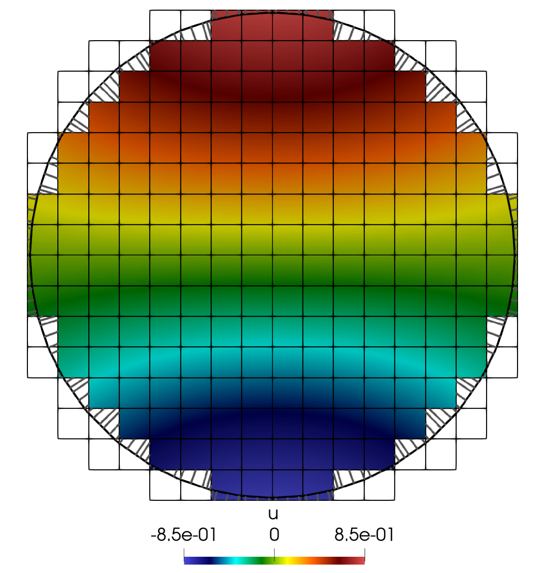
Figure 4: Left: Exemplary numerical solution for the Poisson equation on a unit disc domain, visualized on the surrogate domain ($\lambda=0.75$), obtained with the DG-SBM multigrid method. The true boundary $\Gamma$ is shown in black lines; connections between quadrature points ($p=2$) on the surrogate boundary and their projections on the true boundary are illustrated with grey lines. Note that with $\lambda=0.75$, some parts of the true boundary lie within the surrogate domain Right: Illustrative distribution of minimum and maximum shift magnitudes (normalized by cell size $h$) on the surrogate boundary for the unit disk problem with $p=3$. The values $\pm\sqrt{2}$ represent the theoretical maximum possible normalized shift magnitude in 2D for a square cell.

5.1 Convergence rates

We first verify convergence rates using a manufactured solution approach. For the Poisson equation on the unit sphere $\Omega=\{\mathbf{x}\in\mathbb{R}^{d}\;:\;\|\mathbf{x}\|<1\}$, we choose the manufactured solution

$$u(\mathbf{x})=2\cos(x_{1})\sin(x_{2}),$$

from which we derive the source term $f=-\Delta u$ and Dirichlet boundary condition $g=u|_{\Gamma}$.

For a DG method using piecewise polynomials of degree $p$, we expect to observe optimal convergence rates of order $\mathcal{O}(h^{p+1})$ in the $L_{2}$ norm, provided the solution is sufficiently smooth. Figure 5 shows the $L_{2}$ error versus the mesh size $h$ for different polynomial degrees $p$ in 2D. The shaded regions in the 2D plot (Figure 5) represent the range of $L_{2}$ errors obtained for different values of the threshold parameter $\lambda\in\{1.0,0.75,0.5,0.25\}$, which determines the active cells. It was demonstrated in [44] that the SBM may not yield stable convergence rates for $\lambda=0$. Within this range, lower values of $\lambda$ typically lead to lower $L_{2}$ errors.

The results demonstrate that the DG-SBM method achieves the expected optimal convergence rates of order $\mathcal{O}(h^{p+1})$ in the $L_{2}$ norm for the 2D case across these $\lambda$ values. The dashed lines, representing theoretical convergence rates, align well with the computed errors for polynomial degrees $p=1$ through $p=3$.

Figure 5: Influence of threshold $\lambda$ on $L_{2}$ error for the DG-SBM with $p=1,2,3$ on the unit sphere domain in 2D. Shaded regions show the range of $L_{2}$ errors for $\lambda\in\{0.25,0.5,0.75,1.0\}$. Dashed lines indicate theoretical optimal convergence rates.

5.2 Multigrid for linear elements in 2D

An efficient multigrid preconditioner should ideally exhibit $h$-independence, where the number of iterations for convergence remains relatively constant as the mesh is refined. We investigate this for the Poisson problem on the unit sphere. Figure 6 shows the number ofMG-GMRES iterations versus mesh refinement for linear elements ($p=1$). The left panel displays results for the 2D case, while the right panel shows the corresponding results for the 3D case, both for various threshold values $\lambda$.

For $p=1$ in 2D (left panel), the iteration counts show a mild increase with mesh refinement for all tested $\lambda$ values. For $\lambda=1.0$, iterations increase from 7 to 16 as the mesh is refined from level 1 to 7. Smaller $\lambda$ values generally lead to lower and more stable iteration counts; for instance, with $\lambda=0.25$, iterations range from 5 to 8. In 3D (right panel), a similar trend is observed for $p=1$. Iteration counts increase mildly with refinement. For $\lambda=1.0$, iterations go from 5 to 12 across levels 1 to 4. Again, smaller $\lambda$ values like $\lambda=0.25$ yield more stable and lower iteration counts, ranging from 5 to 6. These results suggest that for linear elements, the multigrid preconditioner provides good scalability with mesh refinement in both 2D and 3D, with lower $\lambda$ values (which include more intersected cells) generally leading to better solver performance.

Figure 6: Convergence of GMRES: iteration counts with $h$-refinement for the SBM with different thresholds $\lambda$ and $p=1$ Left: 2D. Right: 3D.

5.3 Higher order elements

For polynomial degrees $p>1$, we employ a $p$-multigrid strategy. This approach uses the finest geometric mesh with the desired polynomial degree $p$ and creates additional multigrid levels by systematically reducing the polynomial degree down to $p=1$. Since the underlying geometric mesh remains the same across these $p$-multigrid levels, the same set of active cells is considered on each level, ensuring geometric consistency throughout the hierarchy. This $p$-coarsening ensures that the finite element spaces are properly nested across multigrid levels, which allows us to test the effectiveness of the smoother.

Figure 7 presents the GMRES iteration counts for polynomial degree $p=2$ under mesh refinement for the unit sphere problem in 2D (left panel) and 3D (right panel). In 2D, the iteration counts for $p=2$ show good $h$-independence, particularly for $\lambda=0.75$ and $\lambda=1.0$, where iterations remain around 8–11. For $\lambda=0.5$, iterations are also stable, increasing slightly from 6 to 10. However, for $\lambda=0.25$, the solver performance degrades significantly at finer refinement levels, with iteration counts jumping to 28 at level 5 and failing at level 6. This highlights the sensitivity to $\lambda$ for $p=2$ even in 2D. In 3D, for $p=2$, the iteration counts generally show a rease with refinement for $\lambda=0.75$ (6–9 iterations) and $\lambda=0.5$ (5–8 iterations). For $\lambda=1.0$, iterations increase from 7 to 13. The case $\lambda=0.25$ shows stable low iterations (5–6) up to level 3, but then jumps to 14 iterations at level 4. Overall, the $hp$-multigrid preconditioner performs reasonably well for $p=2$, though the choice of $\lambda$ remains important.

The performance for cubic elements ($p=3$) is shown in Figure 8. For these tests, the relaxation parameter for the cell-wise SSOR smoother was set to $\omega=0.8$, as the standard $\omega=1.0$ often led to divergence. In 2D (left panel), for $p=3$ with $\omega=0.8$, the behavior is mixed. For $\lambda=0.75$, iteration counts are relatively stable, increasing from 10 to 14. However, for $\lambda=1.0$, iterations grow significantly with refinement, reaching 57 at level 7. For $\lambda=0.5$, after an initial dip, iterations increase to 43 and then 78. For $\lambda=0.25$, the solver fails at level 5. This indicates increased difficulty for $p=3$ in 2D. In 3D (right panel), the challenges with $p=3$ are more pronounced. For $\lambda=1.0$ and $\lambda=0.25$, the solver fails (100 iterations) already at the second refinement level. For $\lambda=0.75$, iterations are erratic (43, 11, 24). For $\lambda=0.5$, iterations increase from 9 to 11, then jump to 51 at level 3. These results suggest that the current smoother is less effective for $p=3$, especially in 3D, even with a tuned relaxation parameter. Due to prohibitive memory requirements for $p\geq 3$, computations on finer grids for $p=3$ in 3D were not feasible, making it difficult to draw definitive conclusions about the solver’s scalability to finer meshes at this polynomial degree.

Numerous attempts were made to improve the convergence for $p=3$ elements, particularly in 3D. These included exploring additive cell-wise smoothers (block Jacobi) as an alternative to the successive (block Gauss-Seidel) approach. Furthermore, to address the challenge of selecting an optimal relaxation parameter for these additive smoothers, they were wrapped within a Chebyshev polynomial smoother. The Chebyshev smoother can automatically determine a suitable relaxation schedule based on estimates of the estimate of eigenvalues of the preconditioned operator. Despite these efforts, significant improvements in iteration counts for $p=3$ cases, especially in 3D, were not consistently observed.

Figure 7: Convergence of GMRES: iteration counts with $h$-refinement for the SBM with different thresholds $\lambda$ and $p=2$ Left: 2D. Right: 3D.

Figure 8: Convergence of GMRES: iteration counts for the SBM with different thresholds $\lambda$ on a sequence of successively refined meshes, for polynomial degree $p=3$, with relaxation parameter $\omega=0.8$. Left: 2D, Right: in 3D.

5.4 Complex geometry test case

While the unit sphere provides a valuable test case for verifying convergence rates and basic multigrid performance, it is also important to evaluate the method on problems with more complex geometries, where the SBM and the multigrid preconditioner face greater challenges.

Here, we present results for the Poisson equation on a 2D domain with a non-spherical, deformed boundary. This serves as a more challenging test for the SBM, particularly for the closest point projection algorithm which, for such geometries, relies on the local nonlinear solver described in Section 4.2.

Our test domain $\Omega$ is defined by the zero level set of the function

$$\phi(x,y)=\left(1-\frac{3}{4}\sin(\pi x)^{2}\right)(x^{2}+y^{2})-\frac{1}{5},$$

where $\Omega=\{\mathbf{x}\mid\phi(\mathbf{x})<0\}$. The visualization (Figure 9, left panel) illustrates all cells of the background mesh that are at least partially inside $\Omega$. However, only those cells where the fraction of their area inside $\Omega$ exceeds the threshold $\lambda=0.5$ are considered active. The solution is consequently visualized on this set of active cells, which constitute the surrogate domain $\tilde{\Omega}$. It is worth noting that even for the mesh depicted, which is not the coarsest level used in computations, the cell diameter can be larger than the smallest radius of curvature of the domain. Consequently, once can expect that the geometry will not be fully resolved on the coarsest multigrid levels. The DG-SBM method handles the intricate boundary features, and the grey lines depict the shifts from the surrogate boundary to the true boundary.

To assess the convergence behavior of the DG-SBM method, particularly in the presence of a complex, implicitly defined boundary, we employ a manufactured solution directly related to the level set function. We define the exact solution as $u(\mathbf{x})=\phi(\mathbf{x})+1$. Consequently, the source term for the Poisson equation is $f=-\Delta u=-\Delta\phi$. The Dirichlet boundary condition on $\Gamma=\{\mathbf{x}\mid\phi(\mathbf{x})=0\}$ is $g=u|_{\Gamma}=1$.

This choice of a constant boundary condition is particularly insightful. Any inaccuracies in the geometric representation of the boundary $\Gamma$ (e.g., due to approximating the level set function $\phi$ with finite elements) will result in the constant boundary condition $g=1$ being enforced at slightly perturbed locations. These geometric perturbations directly influence the computed solution $u_{h}$ and are thus reflected in the observed convergence rates.

We compute the $L_{2}$ error $\|u-u_{h}\|_{L_{2}(\tilde{\Omega})}$ on the surrogate domain $\tilde{\Omega}$ for a sequence of uniformly refined meshes, and the results of this convergence study are presented in the right panel of Figure 9. We note that for $p=3$ the MG-GMRES solver failed to converge for some $\lambda$ values, leading to a lack of data for these cases. The shaded region for $p=3$ is constructed using data from the subset of $\lambda$ values for which the solver converged at each respective refinement level.

The plot shows that while optimal convergence rates are generally achieved on finer meshes, convergence on coarser meshes, especially for $p=3$, can initially appear stagnant. This occurs because the geometry is under-resolved by the coarser discretizations. Once the cell size is small enough to resolve the geometry, the optimal rate is achieved. However, when the cell size is comparable to or larger than the local radius of curvature, the discrete problem effectively addresses a smoothed or simplified version of the true boundary. This can lead to an initial, but unreliable, rapid error reduction until the mesh becomes fine enough to capture the actual geometric details.

We investigate the performance of the multigrid preconditioner for the DG-SBM method on this complex deformed 2D domain. To ensure a robust evaluation across different polynomial degrees for this complex geometry, we employ a full $hp$-multigrid strategy. Figure 10 displays the number of GMRES iterations needed to reduce the relative residual by a factor of $10^{-12}$. The figure illustrates the solver’s behavior under mesh refinement for various polynomial degrees and $\lambda$ values in 2D.

For polynomial degrees $p=1$ (solid lines) and $p=2$ (dashed lines), the multigrid preconditioner demonstrates good scalability with mesh refinement. For $p=1$, iteration counts exhibit only a mild increase with mesh refinement across all tested $\lambda$ values. For $\lambda=0.5$ and $\lambda=0.25$, the iteration counts remain particularly low and stable, generally below 10 iterations even at the finest refinement level (level 7). For $p=2$, iteration counts are higher but still show reasonable scalability, with $\lambda=0.5$ and $\lambda=0.25$ performing best, staying below 16 and 13 iterations respectively. For $p=3$ (dotted lines), the performance is more sensitive to $\lambda$. While $\lambda=0.75$ (green dotted line) shows iteration counts increasing from 15 to 38, and $\lambda=0.5$ (blue dotted line) increases from 9 to a failure at level 7 (100 iterations), other values show more significant growth or earlier failure. Specifically, for $\lambda=1.0$ (red dotted line), iterations grow rapidly, reaching 100 (failure) at level 7. For $\lambda=0.25$ (orange dotted line), the solver fails at level 4. These results for $p=3$ suggest that while the preconditioner can be effective for some $\lambda$ values, its consistent performance for higher polynomial degrees on complex geometries is more dependent on the choice of $\lambda$.

Overall, the results on the complex deformed 2D domain indicate that the DG-SBM multigrid preconditioner can achieve efficient convergence, with iteration counts showing good scalability with mesh refinement for $p=1$ and $p=2$. The choice of the threshold parameter $\lambda$ plays a significant role, especially for higher polynomial degrees, influencing both the accuracy (as seen in Figure 9) and the iterative solver performance.

In summary, the numerical investigations demonstrate that the proposed DG-SBM multigrid preconditioner generally achieves good $h$-independent or mildly $h$-dependent convergence for linear ($p=1$) and quadratic ($p=2$) elements in 2D for both the unit sphere and the complex geometry. The threshold parameter $\lambda$ plays a crucial role. While lower $\lambda$ values typically lead to lower $L_{2}$ errors and often improve solver stability for $p=1$, this trend does not consistently hold for higher polynomial degrees. For $p\geq 2$, smaller $\lambda$ values, even if beneficial for accuracy, can sometimes degrade solver performance, as observed in several test cases. Significant challenges emerge for cubic ($p=3$) elements, particularly for complex geometries, where the current cell-wise SSOR smoother exhibits reduced effectiveness, leading to increased iteration counts or solver failure.

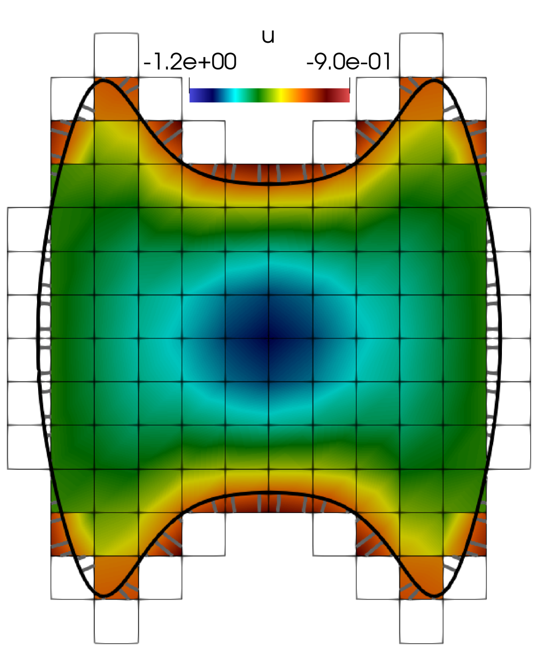
Figure 9: Left: Numerical solution for the Poisson equation on a complex deformed domain, visualized on the surrogate domain ($\lambda=0.5$), obtained with the DG-SBM multigrid method. The true boundary $\Gamma$ is shown in black lines; connections between quadrature points on the surrogate boundary and their projections on the true boundary are illustrated with grey lines. Note that with $\lambda=0.5$, some parts of the true boundary may lie within the surrogate domain. Right: Convergence rate of the DG-SBM method on the same domain.

Figure 10: Convergence of GMRES: iteration counts with multigrid preconditioner for the DG-SBM method on a complex deformed domain in 2D. Solid lines: $p=1$, dashed: $p=2$, dotted: $p=3$. The results are shown for different threshold values $\lambda$.

6 Conclusion

We have developed a geometric multigrid preconditioner for a Discontinuous Galerkin (DG) formulation of the Shifted Boundary Method (SBM), aimed at efficiently solving the Poisson equation on domains with complex boundaries. Numerical results demonstrate that the method, employing a cell-wise SSOR smoother within an $hp$-multigrid framework, achieves good scalability and efficiency for linear ($p=1$) and quadratic ($p=2$) polynomial degrees in 2D.

The choice of the threshold parameter $\lambda$, which defines the set of active cells, significantly impacts solver performance. This sensitivity to $\lambda$ is particularly evident for $p=2$ elements in 3D on complex geometries, where solver stability can be critically affected. The influence of $\lambda$ on iteration counts is nuanced: while smaller $\lambda$ values generally benefit solver performance for linear elements, this trend does not consistently hold for higher polynomial degrees ($p\geq 2$). For these cases, the optimal $\lambda$ for solver efficiency may differ, and smaller $\lambda$ values, even if they improve accuracy, can sometimes degrade solver performance.

Our initial 1D analysis indicated that SBM formulations can lead to system matrices with complex eigenvalues, particularly when the true boundary lies within the surrogate cell (negative shifts). This insight is consistent with numerical findings where smaller threshold values $\lambda$ (e.g., $\lambda=0.25$), which can increase the likelihood of negative shifts, sometimes led to degraded convergence for higher-order elements.

The current cell-wise SSOR smoother shows limitations for higher polynomial degrees, particularly for $p\geq 3$ in 3D, where iteration counts increase substantially or the solver fails to converge. This indicates that the smoothing properties of the cell-wise SSOR are not sufficient for these more challenging SBM discretizations, possibly due to the aforementioned spectral properties becoming more pronounced.

Future work should focus on addressing the limitations observed with the cell-wise SSOR smoother for higher polynomial degrees ($p\geq 3$), particularly in 3D. The development and analysis of more advanced smoothers tailored to the specific properties of DG-SBM systems are crucial. Investigating alternative smoothing strategies, such as Block Jacobi (which was explored, though consistent significant improvements were not observed in the current study without further tuning) potentially with Chebyshev acceleration, could be investigated. A thorough theoretical analysis of the smoother’s properties and its interaction with the SBM formulation is also warranted to guide the design of more effective multigrid components. Furthermore, for higher polynomial degrees, especially when dealing with larger shift distances, modifications to the SBM formulation itself might be necessary to enhance stability and improve smoother performance.

References

- [1] P. C. Africa, D. Arndt, W. Bangerth, B. Blais, M. Fehling, R. Gassmöller, T. Heister, L. Heltai, S. Kinnewig, M. Kronbichler, M. Maier, P. Munch, M. Schreter-Fleischhacker, J. P. Thiele, B. Turcksin, D. Wells, and V. Yushutin, The deal.II library, Version 9.6, Journal of Numerical Mathematics, 32 (2024), pp. 369–380.
- [2] P. F. Antonietti, M. Sarti, and M. Verani, Multigrid algorithms for hp-discontinuous Galerkin discretizations of elliptic problems, SIAM Journal on Numerical Analysis, 53 (2015), pp. 598–618.
- [3] D. Arndt, W. Bangerth, D. Davydov, T. Heister, L. Heltai, M. Kronbichler, M. Maier, J.-P. Pelteret, B. Turcksin, and D. Wells, The deal.II finite element library: Design, features, and insights, Computers & Mathematics with Applications, 81 (2021), pp. 407–422.
- [4] D. N. Arnold, An interior penalty finite element method with discontinuous elements, SIAM journal on numerical analysis, 19 (1982), pp. 742–760.
- [5] N. Atallah, C. Canuto, and G. Scovazzi, Analysis of the shifted boundary method for the Stokes problem, Computer Methods in Applied Mechanics and Engineering, 358 (2020), p. 112609.
- [6] N. Atallah, C. Canuto, and G. Scovazzi, The second-generation shifted boundary method and its numerical analysis, Computer Methods in Applied Mechanics and Engineering, 372 (2020), p. 113341.
- [7] N. Atallah, C. Canuto, and G. Scovazzi, Analysis of the shifted boundary method for the Poisson problem in domains with corners, Mathematics of Computation, 90 (2021), pp. 2041–2069.
- [8] N. Atallah, C. Canuto, and G. Scovazzi, The shifted boundary method for solid mechanics, International Journal for Numerical Methods in Engineering, 122 (2021), pp. 5935–5970.
- [9] N. Atallah, C. Canuto, and G. Scovazzi, The high-order shifted boundary method and its analysis, Computer Methods in Applied Mechanics and Engineering, 394 (2022), p. 114885.
- [10] N. Atallah and G. Scovazzi, Nonlinear elasticity with the shifted boundary method, Computer Methods in Applied Mechanics and Engineering, 426 (2024), p. 116988.
- [11] I. Babuška, The finite element method with penalty, Mathematics of computation, 27 (1973), pp. 221–228.
- [12] S. Badia, E. Neiva, and F. Verdugo, Linking ghost penalty and aggregated unfitted methods, Computer Methods in Applied Mechanics and Engineering, 388 (2022), p. 114232.
- [13] C. E. Baumann and J. T. Oden, A discontinuous hp finite element method for convection—diffusion problems, Computer Methods in Applied Mechanics and Engineering, 175 (1999), pp. 311–341.
- [14] M. Bergbauer, P. Munch, W. A. Wall, and M. Kronbichler, High-performance matrix-free unfitted finite element operator evaluation, arXiv preprint arXiv:2404.07911, (2024).
- [15] J. H. Bramble, J. E. Pasciak, and J. Xu, The analysis of multigrid algorithms with nonnested spaces or noninherited quadratic forms, Mathematics of Computation, 56 (1991), pp. 1–34.
- [16] A. Brandt, Multi-level adaptive solutions to boundary-value problems, Mathematics of computation, 31 (1977), pp. 333–390.
- [17] E. Burman, Ghost penalty, Comptes Rendus. Mathématique, 348 (2010), pp. 1217–1220.
- [18] E. Burman, S. Claus, P. Hansbo, M. G. Larson, and A. Massing, CutFEM: discretizing geometry and partial differential equations, International Journal for Numerical Methods in Engineering, 104 (2015), pp. 472–501.
- [19] E. Burman and P. Hansbo, Fictitious domain methods using cut elements: III. A stabilized Nitsche method for Stokes’ problem, ESAIM: Mathematical Modelling and Numerical Analysis, 48 (2014), pp. 859–874.
- [20] E. Burman, P. Hansbo, and M. G. Larson, On the design of locking free ghost penalty stabilization and the relation to CutFEM with discrete extension, arXiv preprint arXiv:2205.01340, (2022).
- [21] S. Claus and P. Kerfriden, A CutFEM method for two-phase flow problems, Computer Methods in Applied Mechanics and Engineering, 348 (2019), pp. 185–206.
- [22] B. Cockburn, G. E. Karniadakis, and C.-W. Shu, The development of discontinuous Galerkin methods, in Discontinuous Galerkin methods: theory, computation and applications, Springer, 2000, pp. 3–50.
- [23] J. H. Collins, A. Lozinski, and G. Scovazzi, A penalty-free shifted boundary method of arbitrary order, Computer Methods in Applied Mechanics and Engineering, 417 (2023), p. 116301.
- [24] C. Cui and G. Kanschat, Multilevel Interior Penalty Methods on GPUs, arXiv preprint arXiv:2405.18982, (2024).
- [25] S. Gross and A. Reusken, Optimal preconditioners for a Nitsche stabilized fictitious domain finite element method, arXiv preprint arXiv:2107.01182, (2021).
- [26] S. Gross and A. Reusken, Analysis of optimal preconditioners for CutFEM, Numerical Linear Algebra with Applications, 30 (2023), p. e2486.
- [27] C. Gürkan and A. Massing, A stabilized cut discontinuous Galerkin framework for elliptic boundary value and interface problems, Computer Methods in Applied Mechanics and Engineering, 348 (2019), pp. 466–499.
- [28] W. Hackbusch and W. Hackbusch, The Multi-Grid Method of the Second Kind, Multi-Grid Methods and Applications, (1985), pp. 305–353.
- [29] P. Hansbo, M. G. Larson, and K. Larsson, Cut finite element methods for linear elasticity problems, in Geometrically Unfitted Finite Element Methods and Applications: Proceedings of the UCL Workshop 2016, Springer, 2017, pp. 25–63.
- [30] M. Kronbichler and K. Kormann, Fast matrix-free evaluation of discontinuous Galerkin finite element operators, ACM Transactions on Mathematical Software (TOMS), 45 (2019), pp. 1–40.
- [31] D. Kuzmin and J.-P. Bäcker, An unfitted finite element method using level set functions for extrapolation into deformable diffuse interfaces, Journal of Computational Physics, 461 (2022), p. 111218.
- [32] K. Li, N. Atallah, A. Main, and G. Scovazzi, The shifted interface method: a flexible approach to embedded interface computations, International Journal for Numerical Methods in Engineering, 121 (2020), pp. 492–518.
- [33] A. Main and G. Scovazzi, The shifted boundary method for embedded domain computations. Part I: Poisson and Stokes problems, Journal of Computational Physics, 372 (2018), pp. 972–995.
- [34] A. Main and G. Scovazzi, The shifted boundary method for embedded domain computations. Part II: Linear advection–diffusion and incompressible Navier–Stokes equations, Journal of Computational Physics, 372 (2018), pp. 996–1026.
- [35] J. A. Nitsche, Über ein Variationsprinzip zur Lösung von Dirichlet-Problemen bei Verwendung von Teilräumen, die keinen Randbedingungen unterworfen sind, Abhandlungen aus dem Mathematischen Seminar der Universität Hamburg, 36 (1971), pp. 9–15.
- [36] J. T. Oden, I. Babuŝka, and C. E. Baumann, A discontinuoushpfinite element method for diffusion problems, Journal of computational physics, 146 (1998), pp. 491–519.
- [37] W. H. Reed and T. R. Hill, Triangular mesh methods for the neutron transport equation, tech. rep., Los Alamos Scientific Lab., N. Mex.(USA), 1973.
- [38] R. I. Saye, High-order quadrature methods for implicitly defined surfaces and volumes in hyperrectangles, SIAM Journal on Scientific Computing, 37 (2015), pp. A993–A1019.
- [39] M. Wichrowski, Matrix-Free Ghost Penalty Evaluation via Tensor Product Factorization, arXiv preprint arXiv:2503.00246, (2025).
- [40] J. Witte, D. Arndt, and G. Kanschat, Fast tensor product Schwarz smoothers for high-order discontinuous Galerkin methods, Computational Methods in Applied Mathematics, 21 (2021), pp. 709–728.
- [41] D. Xu, O. Colomés, A. Main, K. Li, N. Atallah, N. Abboud, and G. Scovazzi, A weighted shifted boundary method for immersed moving boundary simulations of Stokes’ flow, Journal of Computational Physics, 510 (2024), p. 113095.
- [42] J. Xu, The method of subspace corrections, Journal of Computational and Applied Mathematics, 128 (2001), pp. 335–362.
- [43] T. Xue, W. Sun, S. Adriaenssens, Y. Wei, and C. Liu, A new finite element level set reinitialization method based on the shifted boundary method, Journal of Computational Physics, 438 (2021), p. 110360.
- [44] C.-H. Yang, K. Saurabh, G. Scovazzi, C. Canuto, A. Krishnamurthy, and B. Ganapathysubramanian, Optimal surrogate boundary selection and scalability studies for the shifted boundary method on octree meshes, Computer Methods in Applied Mechanics and Engineering, 419 (2024), p. 116686.
- [45] O. C. Zienkiewicz, R. L. Taylor, S. J. Sherwin, and J. Peiró, On discontinuous Galerkin methods, International journal for numerical methods in engineering, 58 (2003), pp. 1119–1148.
- [46] R. Zorrilla, R. Rossi, G. Scovazzi, C. Canuto, and A. Rodríguez-Ferran, A shifted boundary method based on extension operators, Computer Methods in Applied Mechanics and Engineering, 421 (2024), p. 116782.