Silhouette-Guided Instance-Weighted k-means

Abstract

Clustering is a fundamental unsupervised learning task with numerous applications across diverse fields. Popular algorithms such as k-means often struggle with outliers or imbalances, leading to distorted centroids and suboptimal partitions. We introduce K-Sil, a silhouette-guided refinement of the k-means algorithm that weights points based on their silhouette scores, prioritizing well-clustered instances while suppressing borderline or noisy regions. The algorithm emphasizes user-specified silhouette aggregation metrics: macro-, micro-averaged or a combination, through self-tuning weighting schemes, supported by appropriate sampling strategies and scalable approximations. These components ensure computational efficiency and adaptability to diverse dataset geometries. Theoretical guarantees establish centroid convergence, and empirical validation on synthetic and real-world datasets demonstrates statistically significant improvements in silhouette scores over k-means and two other instance-weighted k-means variants. These results establish K-Sil as a principled alternative for applications demanding high-quality, well-separated clusters.

1 Introduction

Clustering, the process of organizing data into meaningful groups, is a cornerstone of unsupervised learning with broad applications in pattern recognition and data analysis [1]. Among clustering algorithms, k-means [2] remains widely adopted due to its simplicity and scalability. However, its susceptibility to outlier distortion and poor separation in imbalanced clusters frequently results in centroids skewed by noise, producing partitions that misrepresent the underlying data structure, especially in cases with small or overlapping groups [3]. While weighted variants mitigate some limitations, they often lack a principled mechanism to prioritize high-confidence points or suppress unreliable ones [4], limiting their ability to better capture intrinsic data geometries. To address these challenges, we introduce K-Sil, a novel clustering framework that integrates silhouette scores [5, 6], a measure of intra-cluster cohesion and inter-cluster separation, directly into the centroid update process. Unlike traditional k-means, which treats all points uniformly, K-Sil dynamically weights each point based on its silhouette score within its assigned cluster. This approach ensures that well-clustered points, those with strong alignment to their cluster and clear separation from others, exert greater influence on centroid updates, while borderline or noisy points are systemically downweighted. By leveraging silhouette-guided weighting, K-Sil produces centroids that more accurately represent the core of each cluster, yielding partitions that are both more cohesive and better separated.
Overall, the key contributions of this work are: (I) We define clustering objectives guided by silhouette-based aggregation metrics, including the macro-averaged silhouette score for assessing cluster-level separation, the micro-averaged score for evaluating point-wise cohesion, and combinations to balance both aspects, enabling users to prioritize distinct aspects of partition quality. (II) We develop auto-tuned per-cluster weighting schemes that prioritize high-confidence regions and suppress noise or unreliable assignments by leveraging individual silhouette magnitudes (absolute scores) or ranks (relative ordering). (III) We reduce the computational costs of silhouette score calculations using objective-aware sampling, balanced (per-cluster) sampling for macro objectives, uniform for micro, along with centroid-based approximations, scaling to large datasets. (IV) We establish finite convergence under cluster regularity assumptions and validate our algorithm empirically, showing statistically significant silhouette improvements over k-means and other instance-weighted k-means variants across synthetic and real-world datasets. Our code on K-Sil is publicly available at https://github.com/semoglou/ksil and can be installed via PyPI.

2 Related Work

Clustering algorithms are commonly categorized by the strategies they employ, such as partitioning (e.g., k-means [2]), density-based approaches (e.g., DBSCAN [7]), hierarchical clustering [8], model-based methods (e.g., Gaussian Mixture Models [9]), and graph- or spectral-based techniques [10]. These approaches vary in their assumptions, distance metrics, and scalability. In this study, we focus on improving the robustness and structure-awareness of partition-based clustering, particularly k-means, by incorporating dynamic instance-level weighting informed by internal validation signals.

k-means & Weighted Variants

The k-means algorithm [2], introduced by MacQueen in 1967, is one of the most widely used clustering methods due to its efficiency and simplicity. It partitions data into $k$ disjoint clusters by minimizing within-cluster variance using iterative nearest-centroid assignments and centroid updates based on cluster means. Despite its popularity, k-means has several well-known shortcommings. It is highly sensitive to initial centroid placement, often converging to local optima. To improve initialization, methods such as k-means++ [11] and AFKM [12] have been proposed, offering probabilistic or sampling-based strategies that improve stability and convergence. Several variants have also addressed k-means’ sensitivity to outliers and noise. Global optimization approaches like genetic k-means (GKA) [13] and global k-means [14, 15] use evolutionary or incremental strategies to explore better clustering configurations beyond local minima. Moreover, since k-means requires the number of clusters to be known a priori, methods like U-k-means [16] have been introduced to estimate $k$ dynamically during clustering. While these approaches improve optimization or initialization, the fundamental mechanics of k-means remain unchanged as all data points and features contribute equally in clustering. As a result, k-means continues to perform poorly in datasets with outliers, noise or imbalances. Weighted variants aim to mitigate these issues by assigning weights to instances or features, typically based on domain knowledge or heuristics. For example, WK-Means [17] adjusts feature weights based on intra-cluster compactness, while the entropy weighted k-means (EWKM) [18] assigns feature weights based on entropy to address sparse or uniform features. Similarly, the attribute weighting clustering (AWA) method [19] uses variance-based weighting to enhance cluster separation. However, these approaches focus exclusively on features and do not incorporate mechanisms to assess the quality or reliability of individual points. Instance-weighted clustering has also been explored through approaches such as weight-balanced k-means [20], which operates on externally defined weights with cluster size constraints, and methods leveraging density-aware scores like the Local Outlier Factor (LOFKMeans) [21].

Silhouette Integration in k-means

The growing need for structure-aware clustering has led to increased interest in algorithms that incorporate internal validation signals, like the silhouette coefficient [5, 22], not just as evaluation tools, but as guiding components within the clustering process. Some approaches use silhouette-based feedback to iteratively reassign points in order to improve coherence and separation [23]. Other methods, such as WKBSC [24], integrate the silhouette score into the clustering objective by adjusting feature weights within k-means to optimize silhouette. However, most recent silhouette-integrated methods focus exclusively on micro-average silhouette score, overlooking macro-averaged alternatives [3] that better capture structure in imbalanced data. Additionally, commonly used centroid-distance based approximations of the silhouette score, while computationally convenient, may misrepresent local cohesion or separation when not sufficiently correlated with exact values. Silhouette is typically treated as a fixed global objective [24, 25], and while its optimization can enhance metric performance, it may also lead to overfitting, where local irregularities, such as outliers or noise, influence feature weighting in ways that improve the silhouette score but distort the actual clustering structure. These observations highlight the need for alternative strategies that incorporate silhouette guidance in a more localized and interpretable manner, particularly at the instance level, to refine cluster structure without relying solely on global optimization.

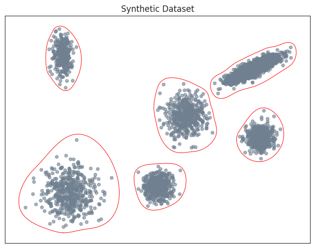
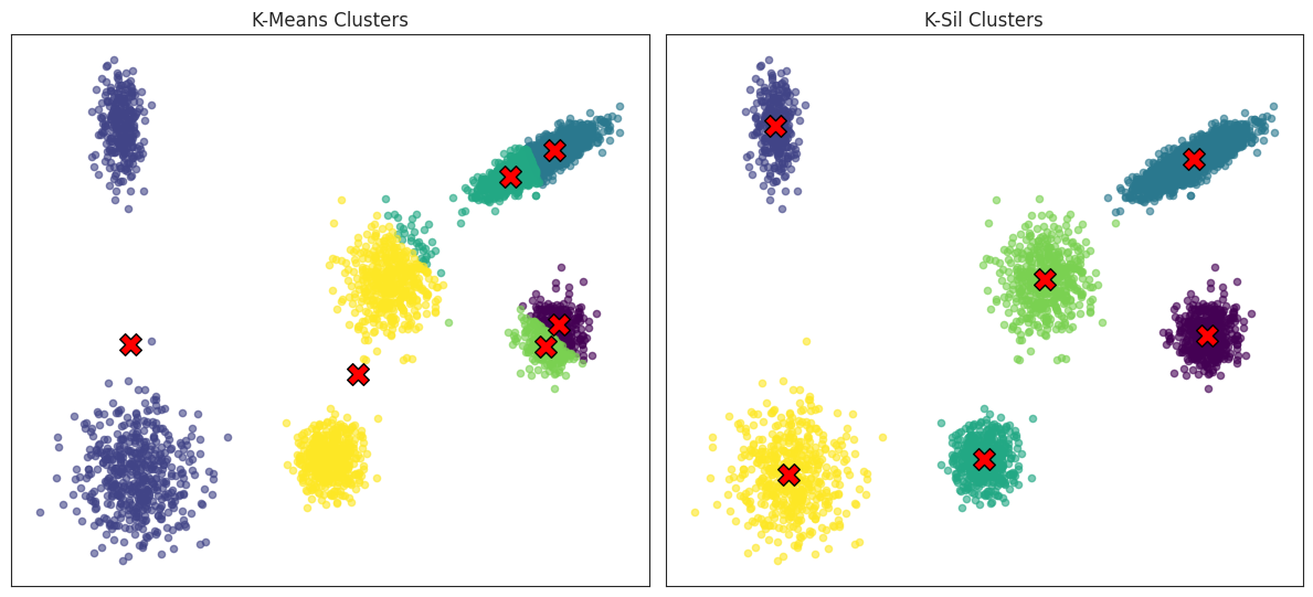
Figure 1: Assignments (and centroids marked in red) produced by k-means (bottom left) and K-Sil (bottom right), both initialized with the same centroids, applied to a synthetic dataset (top) consisting of six distinct clusters with varying densities and sizes (compact spherical clusters, elongated structures, and low-density groups).

3 Methodology

Let $X=\{x_{1},x_{2},\dots,x_{n}\}$ be a dataset consisting of $n$ data points in the metric space $(\mathbb{R}^{d},\ \|\cdot\|)$, where $\|\cdot\|$ denotes the $\ell_{2}$-norm. Given a partition of $X$ into clusters $\{C_{1},\dots,C_{k}\}$, the silhouette score for a point $x_{i}\in C_{j}$, $s(x_{i})$ quantifies the quality of its cluster assignment by comparing its average intra-cluster distance $a(x_{i})$ to its minimum average inter-cluster distance $b(x_{i})$:

$$s(x_{i})=\frac{b(x_{i})-a(x_{i})}{\max\left\{a(x_{i}),b(x_{i})\right\}}\in[-1,1],$$ (1)

$$a(x_{i})=\frac{1}{|C_{j}|-1}\sum_{\begin{subarray}{c}x_{h}\in C_{j}\\ i\neq h\end{subarray}}\|x_{i}-x_{h}\|\ ,\ \ b(x_{i})=\min_{h\neq j}\left\{\ \frac{1}{|C_{h}|}\sum_{x_{m}\in C_{h}}\|x_{i}-x_{m}\|\ \right\}.$$

To evaluate overall clustering quality beyond individual silhouette values and obtain a single summary-metric, we aggregate silhouette scores at the dataset level [3]. We define the micro-averaged silhouette score $S_{\text{m}}$ (the mean of the silhouette scores over all data points) that prioritizes the average quality of individual assignments, particularly effective for datasets with balanced cluster sizes, and the macro-averaged silhouette score $S_{\text{M}}$ (the average of the per-cluster mean silhouette scores) emphasizing performance across clusters, independent of size, suitable for evaluating partitions with imbalanced clusters or when uniform cluster quality is critical:

$$S_{\text{m}}=\frac{1}{n}\sum_{x_{i}\in X}s(x_{i})\ ,\ \ S_{\text{M}}=\frac{1}{k}\sum_{j=1}^{k}\frac{1}{|C_{\text{j}}|}\sum_{x_{i}\in C_{\text{j}}}s(x_{i}).$$ (2)

Clustering Objective

The K-Sil algorithm partitions $X$ into $k\text{ disjoint clusters}$ $\{C_{1},C_{2},\dots,C_{k}\}$ ($k<n$), with corresponding centroids $\{\mu_{1},\mu_{2},\dots,\mu_{k}\}\subset\mathbb{R}^{d}$, through an iterative refinement procedure that maximizes the selected silhouette aggregation objective $S$, either $S_{\text{M}}$, $S_{\text{m}}$ or a convex combination $\alpha S_{\text{m}}+(1-\alpha)S_{\text{M}}$. At each iteration $t$, clusters $C_{j}$ are denoted by $C^{\text{(t)}}_{j}=\{x_{i}\in X:\|x_{i}-\mu^{\text{(t)}}_{j}\|\leq\|x_{i}-\mu^{\text{(t)}}_{h}\|\ \forall h\in\{1,\dots,k\}\}$, where $\mu^{\text{(t)}}_{j}$ denotes the centroid of cluster $C^{\text{(t)}}_{j}$. Also, let $S^{(t)}$ and $s^{(t)}_{i}$ denote the value of the objective and the silhouette score of data point $x_{i}$ at iteration $t$.

Initialization

The algorithm obtains the initial clusters by selecting centroids through a single k-means iteration. The centroids are selected via either random initialization or the k-means$++$ method, which identifies well-separated starting points.

3.1 Iterative Refinement and Centroid Updates

Once the initial clusters are established, the algorithm proceeds with the iterative refinement. At each iteration $t$, the following steps are executed (detailed outline in Appendix A.1).

Silhouette Scores Computation

The algorithm iteratively refines clusters via silhouette scores computed for all data points within each cluster. For large datasets, where computing exact silhouette scores becomes computationally prohibitive due to $O(n^{2})$ pairwise distance calculations, the algorithm offers two options for scalability. First, objective-aligned sampling reduces the number of points evaluated: Uniform sampling preserves proportional cluster representation for the micro-averaged objective $S_{\text{m}}$, while per-cluster sampling enforces equal representation for the macro-averaged objective $S_{\text{M}}$. Second, a silhouette approximation that avoids pairwise distance computations by estimating intra-cluster and inter-cluster distances using cluster sizes, centroids and within clusters sum of squares ($SS$), effectively reducing computational complexity to $O(nk)$ or, when sampling is enabled and the number of sampled points is $m\ (<n)$, to $O(mk)$. Specifically, for each point $x_{i}\in C_{j},\ \text{with}\ j\in\{1,\dots,k\}$, the approximate $\tilde{a}(x_{i})$ and $\tilde{b}(x_{i})$ are defined as:

$$\tilde{a}(x_{\text{i}})=\sqrt{\frac{|C_{\text{j}}|\cdot\|x_{\text{i}}-\mu_{\text{j}}\|^{2}+SS_{C_{\text{j}}}}{|C_{\text{j}}|-1}}\ ,\quad\tilde{b}(x_{\text{i}})=\min_{h\neq j}\sqrt{\|x_{\text{i}}-\mu_{\text{h}}\|^{2}+\frac{SS_{C_{\text{h}}}}{|C_{\text{h}}|}},$$ (3)

where $SS_{C_{j}}=\sum_{x\in C_{j}}\|x-\mu_{j}\|^{2}$, and the approximate silhouette score for $x_{i}\in C_{j}$ is:

$$\tilde{s}(x_{i})=\frac{\tilde{b}(x_{i})-\tilde{a}(x_{i})}{\max\{\tilde{a}(x_{i}),\tilde{b}(x_{i})\}}.$$ (4)

These approximations improve upon the commonly used centroid-distance proxy that can be overly simplistic, by incorporating cluster variability. The approximated $\tilde{a}(x_{i})$ accounts for both the point-to-centroid distance and the overall spread of the cluster, providing a more accurate estimation of the true average intra-cluster distance. Similarly, the approximation of $\tilde{b}(x_{i})$ considers the proximity to neighbouring cluster centroids along with their internal dispersion, reducing the risk of overestimating separation in high-variance clusters. Although the absolute values of the approximated scores may differ slightly from those obtained via exact calculations, their relative ordering and thus the overall silhouette behavior remains reliably consistent (see also Appendix Tables 3 and 4 for correlation analysis with exact silhouette scores and comparisons against simpler centroid-distance-based approximations).

Instance Weighting

Within each cluster $C^{\text{(t)}}_{j}$, (sampled) points are assigned weights based on their silhouette scores to prioritize well-clustered regions and de-emphasize low-silhouette points during centroid updates. Two weighting schemes are employed, each with distinct advantages depending on cluster homogeneity:

• Power Weighting Scheme: For $x_{i}\in C^{\text{(t)}}_{j}$, the weight $w^{\text{(t)}}_{i}=w(x_{i})$ is defined as:

  $$w^{\text{(t)}}_{i}=\left[\frac{s^{\text{(t)}}(x_{i})-s_{\text{min}}(C^{\text{(t)}}_{j})+\epsilon}{\text{Median}\left(\left\{(s^{\text{(t)}}(x_{h})-s_{\text{min}}(C^{\text{(t)}}_{j})+\epsilon)\ |\ x_{h}\in C^{\text{(t)}}_{j}\right\}\right)}\right]^{p},$$ (5)

  where $s_{\text{min}}(C^{\text{(t)}}_{j})$ is the minimum silhouette score in $C^{\text{(t)}}_{j}$, $\epsilon$ is a small constant ensuring numerical stability and $p>0$ is a weight sensitivity parameter controlling the weight contrast. This scheme amplifies deviations from the minimum silhouette, median-scaled, making it effective for homogeneous clusters where absolute silhouette differences reliably distinguish core points from noise.

• Exponential Weighting Scheme: For $x_{i}\in C^{\text{(t)}}_{j}$, the weight $w^{\text{(t)}}_{i}=w(x_{i})$ is defined as:

  $$w^{\text{(t)}}_{i}=\exp\left[-p\cdot\frac{\text{rank}\left(s^{\text{(t)}}(x_{i})\right)-\text{Median}\left(\left\{\text{rank}\left(s^{\text{(t)}}(x_{h})\right)\ |\ x_{h}\in C^{\text{(t)}}_{j}\right\}\right)}{\text{rank}(s_{\text{min}}(C^{\text{(t)}}_{j}))\ /\ 2}\right],$$ (6)

  where $\text{rank}\left(s^{\text{(t)}}(x_{i})\right)$ is the descending dense rank of $s^{\text{(t)}}(x_{i})$ among the silhouette scores of other points in $C^{\text{(t)}}_{j}$ (points with higher silhouette scores receives lower ranks; tied scores share the same rank), $\text{rank}(s_{\text{min}}(C^{\text{(t)}}_{j}))$ is the maximum rank in $C^{\text{(t)}}_{j}$, corresponding to the rank of the cluster’s minimum silhouette score point and $p>0$ is a weight sensitivity parameter that controls the exponential decay rate (centered around the median). This scheme emphasizes rank-based deviations from the median, normalized relative to each cluster, making it robust in heterogeneous clusters (e.g., variable densities) and well-suited to silhouette approximations (Eq. 4), where relative positioning is more reliable than absolute values.

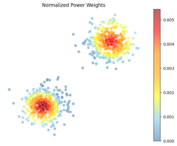
(a) Power weights

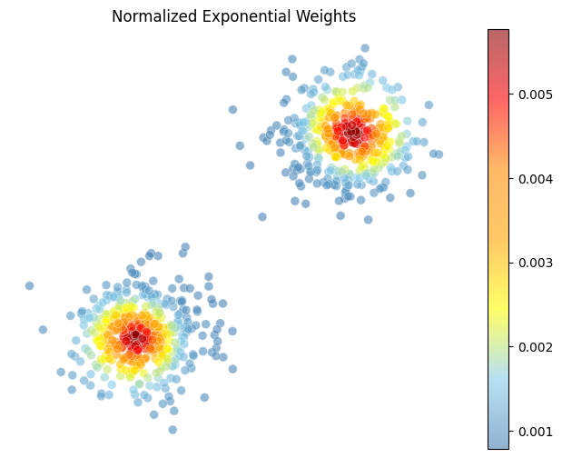
(b) Exponential weights

Figure 2: Normalized instance weights from the power (left) and exponential (right) weighting schemes (each configured with a weight sensitivity factor) on synthetic data of two Gaussian clusters (800 samples, $\sigma=1.3$).

Centroid Updates and Convergence

After assigning weights to points in each cluster, the algorithm updates centroids to reflect the weighted influence of points. For each cluster $C^{\text{(t)}}_{j}$, the new centroid $\mu^{\text{(t+1)}}_{j}$ is computed as:

$$\mu^{\text{(t+1)}}_{j}=\frac{\sum_{x_{i}\in C^{\text{(t)}}_{j}}w^{\text{(t)}}_{i}x_{i}}{\sum_{x_{i}\in C^{\text{(t)}}_{j}}w^{\text{(t)}}_{i}}.$$ (7)

This weighted average ensures centroids shift toward regions of high silhouette scores, enhancing cluster compactness and separation. If a cluster $C^{\text{(t)}}_{j}$ becomes empty during point reassignment after the centroid update, it is re-initialized by selecting the point farthest from the centroid of the largest cluster (by size), denoted $C^{\text{(t)}}_{\text{max}}$ (discussion on the re-initialization strategy in Appendix A.3). Formally, the re-initialized centroid would be:

$$\mu^{\text{(t+1)}}_{j}=\arg\max_{x\in C^{\text{(t)}}_{\text{max}}}\|x-\mu^{\text{(t)}}_{\text{max}}\|.$$ (8)

Finally, the algorithm terminates when the average centroid movement falls below a threshold $\tau$, $\left[\frac{1}{k}\sum_{j=1}^{k}\|\mu^{\text{(t+1)}}_{j}-\mu^{\text{(t)}}_{j}\|<\tau\right],$ or a maximum iteration limit is reached, and the partition (centroids, labels) with the highest observed silhouette objective $S^{*}$ across all iterations is retained. As will be demonstrated in the upcoming Analysis (§4), K-Sil’s weighted centroid updates increase the modified weighted-silhouette objective $F$ (Eq. 10) until convergence. However, because instance weights $w^{(t)}_{i}$ adapt at every iteration, there can be scenarios where the final iterations further refine the modified weighted objective $F^{(t)}$ by adjusting centroids toward highly-weighted regions. This refinement can narrow cluster separations and consequently reduce the unweighted macro- or micro-averaged silhouette scores, resulting in a correlation divergence between $F$ and $S_{M}\text{ or }S_{m}$ in the final updates of the algorithm. In such cases, the unweighted silhouette may reach its maximum at an earlier iteration prior to convergence. Recording the unweighted silhouette score $S^{(t)}$ at each step and retaining the labels corresponding to its maximum $S^{*}$ effectively mitigates the risk of overfitting to the weighted objective $F$, ensuring that the final output remains faithful to the original silhouette-based clustering goal. Additionally, even when the retained clustering corresponds to an intermediate iteration rather than the final one, it is not an unstable or noisy partition. Since low-silhouette points contribute negligibly to centroid updates due to their small weights, they cannot falsely drive a silhouette spike. The inherent robustness of the silhouette-based instance-weighting ensures that high-silhouette partitions reflect genuinely stable and well-separated structures, not effects of noise or short-lived configurations.

3.2 Weight-Sensitivity Parameter

The weighting schemes in K-Sil are designed to amplify the influence of points with high silhouette scores while suppressing those with low ones. This is achieved through a weight-sensitivity parameter $p$, which directly controls the contrast between weights assigned to well-clustered and poorly clustered points within each cluster. For both weighting schemes, points with scores above the median silhouette in each cluster, receive weights $>1$, amplifying their contribution to centroid updates. Conversely, points below the median receive weights $<1$, reducing their influence. The parameter $p$ scales this contrast, by defining the distinction between high and low silhouette regions. Increasing $p$ sharpens contrasts, prioritizing high-confidence points, while decreasing $p$ softens distinctions, retaining borderline regions. It is either auto-tuned via grid search over a predefined range to maximize the selected silhouette objective ($S_{\text{M}},\ S_{\text{m}}$ or their combination) or set to a fixed value for efficiency in time-sensitive applications (silhouette score variation across sensitivity values is depicted in the following plots).

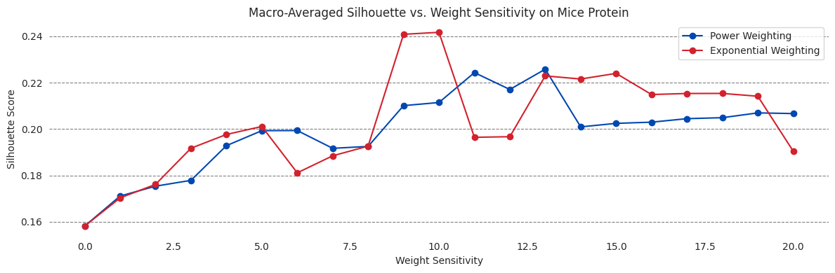
(a) Mice Protein

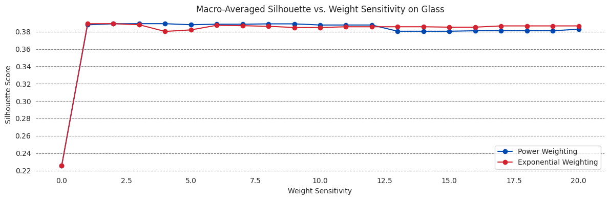
(b) Glass

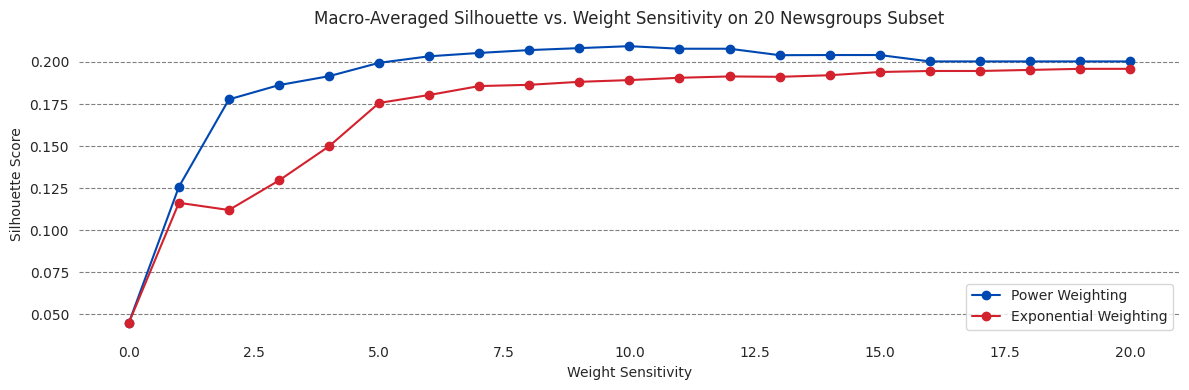
(c) 20 Newsgroups Subset

Figure 3: K-Sil’s performance on macro-averaged silhouette score across the weight sensitivity parameter (0-20, where $p=0$ corresponds to the highest silhouette k-means partition of its clustering run). Blue: power weighting, red: exponential weighting. Evaluated on the Mice Protein dataset, Glass dataset, and a 20 Newsgroups subset.

4 Theoretical Analysis

We establish theoretical guarantees for the K-Sil algorithm, emphasizing centroid convergence in finite time under assumptions (see Appendix B for detailed derivations).

4.1 Cluster Partitioning by Silhouette Scores

Given that $C^{\text{(t)}}_{j}$ represents the $j$-th cluster at iteration $t$ with centroid $\mu^{\text{(t)}}_{j}$, we analyze its structure by partitioning points based on their silhouette scores.
Using $m^{\text{(t)}}_{j}=\text{Median}\left(\left\{s^{(t)}(x_{\text{i}})\ |\ x_{\text{i}}\in C^{\text{(t)}}_{\text{j}}\right\}\right)$, the median silhouette score of all points in $C^{\text{(t)}}_{j}$, we partition each cluster into two key subsets to analyze the algorithm’s behavior: $H^{\text{(t)}}_{j}$, the subset of high-silhouette (core) points that are strongly aligned with their cluster, and drive centroid updates due to their high weights ($>1$), and $L^{\text{(t)}}_{j}$, the subset of low-silhouette (peripheral or borderline) points that lie farther from the cluster’s core, including noisy instances or even outliers, and contribute minimally to centroid updates due to their low weights ($<1$):

$$H^{\text{(t)}}_{j}=\left\{x_{i}\in C^{\text{(t)}}_{j}\ |\ s^{\text{(t)}}(x_{i})>m^{\text{(t)}}_{j}\right\},\ L^{\text{(t)}}_{j}=\left(C^{\text{(t)}}_{j}\setminus H^{\text{(t)}}_{j}\right).$$ (9)

The distinction between core and peripheral points reflects the intrinsic quality of cluster assignments, with core points representing high-confidence regions.

4.2 Assumptions

Our analysis relies on a set of assumptions and properties which, while reflecting idealized conditions, offer a clear framework of the algorithm’s behavior.

• At each iteration $t$, clusters $C^{\text{(t)}}_{j}$ form convex sets, and well-clustered points $H^{\text{(t)}}_{j}$ lie within the convex hull of their points (concentrated near the centroid), ensuring centroids evolve within well-defined, dense regions, avoiding erratic shifts.

• The total weight of high-silhouette score points exceeds that of low-silhouette ones: $\sum_{x_{i}\in H^{\text{(t)}}_{j}}w_{i}\geq\gamma\cdot\sum_{x_{i}\in C^{\text{(t)}}_{j}}w_{i},\text{ with }\gamma>0.5$. This arises naturally from the weighting schemes, which prioritize points above the median silhouette score.

• Centroid movements $\Delta\mu_{j}^{\text{(t)}}=(\mu_{j}^{\text{(t+1)}}-\mu_{j}^{\text{(t)}})$ align directionally with well-clustered points: $\Delta\mu_{j}^{\text{(t)}}\cdot(x_{i}-\mu^{\text{(t)}}_{j})\geq 0\ \forall x_{i}\in H^{\text{(t)}}_{j},\ j\in\{1,\dots,k\}$, reducing intra-cluster distances for these points and preserving compactness. A property that is a direct outcome of the weighted mean update, which pulls centroids toward core regions.

• For every pair of distinct clusters $C^{\text{(t)}}_{j},\ C^{\text{(t)}}_{h}\text{ with }j\neq h$, centroid updates do not systematically reduce inter-centroid distances: $\|\mu^{\text{(t+1)}}_{j}-\mu^{\text{(t+1)}}_{h}\|\geq\|\mu^{\text{(t)}}_{j}-\mu^{\text{(t)}}_{h}\|$ (based on weighting schemes, the centroids move toward their respective high-silhouette regions, not toward other clusters).

• Silhouette scores change smoothly with centroid positions, small centroid movements induce bounded changes in silhouette scores. A Lipschitz constant $L$ quantifies this relationship: $|s^{\text{(t+1)}}(x_{i})-s^{\text{(t)}}(x_{i})|\leq L\|\mu^{\text{(t+1)}}_{j}-\mu^{\text{(t)}}_{j}\|$, where $s^{\text{(t)}}(x_{i})$ represents the silhouette score of a point $x_{i}\in C^{\text{(t)}}_{j}$ at iteration $t$.

4.3 Key Findings

Stability of High-Silhouette Regions $H^{\text{(t)}}_{j}$

Points in $H^{\text{(t)}}_{j}$, maintain or improve their scores across iterations. This occurs because weighted centroid updates shift centroids toward these high-confidence points, reducing their intra-cluster distances (3). Simultaneously, cluster separation (4) ensures inter-cluster distances do not diminish, preserving silhouette score gains. Stability of membership in $H^{\text{(t)}}_{j}$ follows from controlled shifts in the median silhouette score. Centroid movements, constrained by the dominance of high-silhouette weights (2), induce only gradual changes to the median. This ensures the gap between a point’s silhouette score and the median remains sufficient to retain its classification in $H^{\text{(t+1)}}_{j}$. Thus, high-silhouette regions evolve predictably, maintaining their core structure (full derivations are provided in Appendix B.1).

Objective Function and Convergence

K-Sil is designed to optimize Silhouette (either $S_{\text{M}}$ or $S_{\text{m}}$), however, random drips in silhouette might occur across iterations, given its convex nature. Thus, we will use a modified version of Silhouette as the objective function that ensures convergence in a finite number of iterations and preserving the insights of silhouette metrics:

$$F=F^{\text{(t)}}=\sum_{j=1}^{k}\sum_{x_{i}\in C^{\text{(t)}}_{j}}w^{\text{(t)}}_{i}\cdot s^{\text{(t)}}(x_{i}).$$ (10)

The objective is inherently bounded because silhouette scores lie within $[-1,1]$ (or $[0,1]$ for non-trivial clusters), and the total weight across all points is fixed.
Monotonic improvement is guaranteed because updates focus on refining high-confidence regions—centroid adjustments reduce intra-cluster distances for core points, improving their scores, while borderline points contribute minimally due to their low weights. Degradation of stable regions is prevented by directional centroid updates (3) and cluster separation (4), which restrict erratic centroid shifts and preserve cluster boundaries. Since $F$ is non-decreasing and bounded, the sequence of objective values stabilizes once centroid movements become negligible. Combined with the finite number of possible cluster configurations, this ensures the algorithm terminates in a finite number of iterations, converging to a locally optimal partition (a detailed analysis of these properties is provided in Appendix B.2).

5 Empirical Validation

To evaluate K-Sil we conducted experiments on both synthetic and real-world datasets, covering a range of clustering challenges such as varying densities, high-dimensional spaces, noisy structures and non-convex shapes. Synthetic datasets included: S1 (500 points distributed across 5 clusters of varying densities), S2 (500 points in 5 clusters of $\sigma=1$ within a 12-dimensional space), S3 (similar to S2 with an increased cluster spread, $\sigma=2.5$) and S4 (1500 points, combining a circular cluster, a line, and 50% noise). Real-world datasets comprised: Iris (150 samples of 4 numerical features, of 3 flower species), Mice Protein (1080 samples from 8 conditions, with 77 protein features), Glass (214 instances of 6 glass types, described by 9 elemental compositions), Wine (178 samples of 13 chemical attributes, from three wine types), Digits (1797 images of 64 pixel values, of handwritten digits 0-9) and a 20 Newsgroups Subset (2389 text documents from 4 overlapping categories). High-dimensional data were reduced via PCA (retaining $\geq$ 90% of variance), text was TF-IDF vectorized and numerical features were standardized. All real-world datasets are publicly available from UCI or scikit-learn  [26, 27].

Set-Up

To assess performance, we evaluate K-Sil against standard k-means, and two other instance-weighted variants. First, our own implementation of LOFKMeans [21], which weights points based on Local Outlier Factor (LOF) scores; points identified as likely outliers receive lower weights, while those in denser regions receive higher weights, thereby reducing the influence of noisy or ambiguous samples on centroid updates.
Second, DensityKMeans, our instance-weighted k-means baseline, which estimates each point’s local density as the average distance to its $h$ nearest neighbours and sets its weight to the inverse of this estimate: $w_{i}=\left(\frac{1}{h}\sum_{\mathbf{x}_{j}\in\mathcal{N}_{h}(\mathbf{x}_{i})}\|\mathbf{x}_{i}-\mathbf{x}_{j}\|+\epsilon\right)^{-1}$, where $\mathcal{N}_{h}(x_{i})\text{ is the set of }h\text{ neighbours of }x_{i}$ and $\epsilon$ is a small stability constant. We designed DensityKMeans to better capture the inherent structure of datasets with varying densities by emphasizing points located in denser regions and reducing the contribution of those in sparser areas. All algorithms were initialized from the same centroids to ensure a fair comparison. Additionally, when comparing silhouette score performance, we tune the neighborhood size parameters of both LOFKMeans (number of neighbours used to calculate the LOF scores) and DensityKMeans (number of neighbours used to compute local densities) via grid search, selecting those that maximize the chosen silhouette objective ($S_{M}$ or $S_{m}$). Clustering performance is assessed using the Wilcoxon signed-rank test [28] on silhouette values, comparing K-Sil against each baseline. First, we evaluate across a range of cluster counts ($k\in\{2,\dots,10\}$), running multiple trials per $k$ and computing paired differences in silhouette scores between K-Sil and the other algorithms. The test determines whether these differences consistently favour K-Sil; when significance is confirmed ($p$-value $<0.05$), we report the mean relative silhouette improvement (%) across all $k$. Second, we repeat this procedure using only the ground-truth number of clusters $k_{\text{GT}}$, to assess performance under optimal conditions. In both cases, we apply this test separately for macro-averaged ($S_{M}$) and micro-averaged ($S_{m}$) silhouette scores, depending on the K-Sil configuration being evaluated. Additionally, to validate external clustering quality, we compare average NMI scores along with 95% confidence intervals (computed using the t-distribution) for each algorithm on synthetic datasets, where true labels are known by construction.

Table 1: Statistically significant ($p$-value $<0.05$) average relative improvements (%) in macro-averaged silhouette $S_{M}$ of K-Sil (configurations for each dataset in Appendix 5) over baselines across $k\in\{2,\dots,10\}$ (with values in parentheses indicating the average relative improvement computed only at the ground-truth number of clusters $k_{GT}$). “-”indicates a statistically insignificant difference.

Dataset	Average Relative Improvements in $S_{M}$ of K-Sil
	over k-means	over DensityK-Means	over LOFK-Means
S1	7.73% (2.55%)	7.25% (4.95%)	4.27% (1.29%)
S2	46.60% (42.56%)	6.46% (-)	5.63% (-)
S3	30.43% (47.32%)	15.16% (-)	6.70% (-)
S4	16.29% (28.22%)	24.25% (24.50%)	12.32% (27.35%)
Iris	13.35% (1.66%)	6.26% (-)	9.22% (1.26%)
Mice Protein	42.41% (45.80%)	39.57% (48.60%)	29.24% (34.29%)
Glass	42.31% (50.25%)	66.05% (62.83%)	34.36% (36.55%)
Wine	4.03% (-)	5.10% (1.01%)	3.02% (-)
Digits	5.71% (9.02%)	15.78% (23.43%)	32.47% (28.08%)
20 Newsgroups	197.13% (254.05%)	- (-)	212.65% (220.33%)

Table 2: Statistically significant ($p$-value $<0.05$) average relative improvements (%) in $S_{M}$ of K-Sil, using approximate silhouette scores, over baselines across $k$ (with values in parentheses indicating the average relative improvement computed only at the ground-truth number of clusters $k_{GT}$). “-”indicates a statistically insignificant difference.

Dataset	Average Relative Improvements in $S_{M}$ of K-Sil
	over k-means	over DensityK-Means	over LOFK-Means
S1	10.03% (4.29%)	9.55% (6.67%)	6.37% (2.92%)
S2	40.18% (71.22%)	- (-)	- (-)
S3	31.95% (72.85%)	16.21% (-)	7.77% (-)
S4	16.83% (23.90%)	24.70% (20.36%)	12.87% (23.09%)
Iris	19.13% (1.58%)	11.69% (0.33%)	14.84% (1.16%)
Mice Protein	79.95% (74.35%)	75.66% (77.53%)	61.68% (59.90%)
Glass	48.95% (40.02%)	68.29% (53.67%)	40.37% (29.09%)
Wine	4.55% (-)	5.64% (-)	3.49% (-)
Digits	3.77% (9.46%)	13.20% (23.84%)	29.77% (28.47%)
20 Newsgroups	183.57% (237.74%)	- (-)	200.16% (192.32%)

Figure 4: Average NMI scores with 95% (t-distribution) confidence intervals (error bars) of K-Sil (macro- and micro-silhouette modes), k-means, DensityKMeans, and LOFKMeans on synthetic datasets. LOFKMeans used 5 neighbours (scikit-learn default), and DensityKMeans used 10 neighbours for local density estimation, values appropriate for the moderate size and structure of S1-S4.

Empirical Results

K-Sil consistently outperforms standard k-means as well as the other instance-weighted variants in clustering quality, achieving statistically significant improvements across both micro- ($S_{m}$) and macro-averaged ($S_{M}$) silhouette scores.
The most notable gains occur in scenarios where centroid-based partitioning methods is known to struggle: datasets with overlapping clusters, noisy regions, or imbalanced group sizes. Even in non-convex geometries, where all methods face inherent issues (due to reliance on Euclidean distances), K-Sil mitigates some of these limitations by reorienting centroids toward regions with strong cluster cohesion, achieving better separation. The improvements hold not only at the ground-truth number of clusters $k_{\text{GT}}$ but also across misspecified $k$ values, demonstrating robustness to suboptimal parameter choices.
K-Sil’s most substantial improvements occur for the macro-averaged silhouette (when also configured to prioritize it - Table 1), as the algorithm’s cluster-centric weighting strategy that amplifies high-confidence points within each cluster aligns with the macro-silhouette’s emphasis on uniform cluster quality. This makes K-Sil particularly effective for detecting subtle patterns, preserving minority groups, or ensuring equitable representation in heterogeneous data.
The results in Table 1 illustrate K-Sil’s statistically significant improvements in $S_{M}$ over the other algorithms across the synthetic and real-world datasets. While substantial in most cases, a few datasets, such as Wine or certain synthetic ones, exhibit (statistically) insignificant differences, suggesting that when cluster boundaries are already well-defined, structural contrast is low, or the dataset geometry limits the effectiveness of centroid-based partitions, silhouette-based refinement may offer limited additional benefit. Importantly, these improvements are largely preserved when using approximate silhouette scores, as shown in Table 2, with several datasets (e.g., Mice Protein, Glass) even exhibiting greater results, highlighting the robustness and efficiency of the approximation in practice. Additionally, average NMI scores with (t-distribution) 95% confidence intervals on synthetic datasets in Figure 4, show that K-Sil outperforms all baselines in most settings, demonstrating both stronger structural discovery and greater stability.

6 Conclusions

K-Sil enhances k-means by integrating silhouette-guided instance weighting directly into the clustering process, amplifying the influence of high-confidence regions while suppressing noise within each cluster. The algorithm adapts to user-defined objectives, macro-averaged silhouette for balanced cluster quality, micro-averaged for point-level cohesion, or hybrid metrics, while its cluster-centric weighting strategy naturally aligns with macro-averaged silhouette score properties, yielding partitions with improved separation and coherence. By addressing key limitations of k-means, K-Sil demonstrates statistically significant improvements across synthetic and real-world datasets, particularly in noisy, imbalanced and overlapping clusters. To ensure scalability, K-Sil incorporates objective-aware sampling and silhouette approximations, which reduce computational costs while preserving quality. Nevertheless, K-Sil is more computationally intensive than standard k-means due to its iterative weight updates. Its reliance on Euclidean distance may also limit effectiveness on complex or non-Euclidean structures, pointing to potential extensions involving alternative distance metrics. Additionally, although the silhouette-based weighting strategy mitigates some of the issues caused by poor centroid initialization, K-Sil still inherits the sensitivity of centroid-based methods, making multiple runs advisable for robust clustering. Overall, K-Sil offers a principled and adaptable refinement of k-means, particularly in challenging settings where traditional methods struggle. By addressing fundamental limitations of centroid-based methods through silhouette-guided weighting, it achieves more coherent and well-separated clusters. Future work may extend K-Sil with adaptive distance metrics, and scalability enhancements to broaden its applicability.

Appendix A Detailed Methodology

A.1 K-Sil Algorithm Outline

Algorithm K-Sil Clustering

Dataset $X$, number of clusters $k$, and parameters $P$ including:

• Centroid initialization method (random or $k$-means++),

• Chosen Silhouette objective $S$ ($S_{\text{M}}$, $S_{\text{m}}$, or a combination),

• Sampling size,

• Approximation option,

• Centroid movement threshold $\tau$ and Maximum number of iterations,

• Weighting scheme (power or exponential),

• Weight sensitivity parameter value

Final cluster centroids $\mu^{*}$, labels $L^{*}$ and objective score $S^{*}$

$(\mu,L)\leftarrow$ Initial centroids and labels via one $k$-means iteration

$S^{*}\leftarrow(-\ 1)$ (best silhouette objective observed)

$(\mu^{*},L^{*})\leftarrow(\mu,L)$ (centroids and labels corresponding to $S^{*}$)

repeat

  for each cluster $C_{j}$ do

   if  sampling is enabled then

     Let $C^{S}_{j}\subset C_{j}$ be the sampled subset

   else

     Let $C^{S}_{j}=C_{j}$

   end if

   Compute silhouette scores (or approximations) for all $x_{i}\in C^{S}_{j}$

   Assign weights for all $x_{i}\in C^{S}_{j}$ based on weighting scheme—sensitivity value

  end for

  $\mu\leftarrow$ Update cluster centroids using weighted averages

  $L\leftarrow$ Reassign each $x_{i}\in X$ to the nearest centroid

  Reinitialize any empty cluster centroids if necessary

  $\text{score}\leftarrow$ Current silhouette aggregation objective on new Labels $L$

  if $\text{score}>S^{*}$ then

   $S^{*}\leftarrow\text{score}$

   $(\mu^{*},L^{*})\leftarrow$ Current $\mu$ and $L$ (as the best solution)

  end if

until (average centroid movement $<\tau$) or (maximum iterations reached)

return $(\mu^{*},L^{*},S^{*})$

A.2 Evaluation of Silhouette Approximation

To improve scalability in large datasets, K-Sil adopts a silhouette approximation (§ 3.1) that avoids exact pairwise distance computations. Here, we evaluate our refined approximation, denoted as ApR (Eq. 4), against a commonly used simplification, denoted as ApS, that estimates silhouette values based only on distances to centroids. Specifically, for a point $x_{i}\in C_{j}$, ApS defines $a(x_{i})$ as the distance from $x_{i}$ to its assigned centroid $\mu_{j}$, and $b(x_{i})$ as the distance to the nearest centroid of a different cluster, resulting to the silhouette approximation:

$$\tilde{s}(x_{i})=\frac{\min_{h\neq j}\{\|x_{i}-\mu_{h}\|\}-\|x_{i}-\mu_{j}\|}{\max\{\|x_{i}-\mu_{j}\|,\ \min_{h\neq j}\{\|x_{i}-\mu_{h}\|\}\}}.$$

On the datasets used in § 5 (using ground-truth k-means partitions), the refined approximation (ApR) consistently aligns more closely with the exact silhouette scores, both at the individual point level and aggregated metrics, than the simplified baseline.

Table 3: Spearman Rank Correlation $(\rho)$ of ApR and ApS point scores with exact point-silhouette scores. The highest correlation for each dataset is indicated in bold.

Dataset	ApR Correlation ($\rho$)	ApS Correlation ($\rho$)
S1	0.994	0.958
S2	1.000	0.935
S3	0.999	0.985
S4	0.965	0.919
Iris	0.984	0.906
Mice Protein	0.997	0.846
Glass	0.988	0.917
Wine	0.984	0.915
Digits	0.998	0.961
20 Newsgroups	0.979	0.809

Table 4: Comparison of Exact, ApR and ApS aggregated $S_{M/m}$ scores.

Dataset	Exact (Silhouette) Scores		ApR Scores		ApS Scores
	$S_{\text{m}}$	$S_{\text{M}}$	$S_{\text{m}}$	$S_{\text{M}}$	$S_{\text{m}}$	$S_{\text{M}}$
S1	0.576	0.565	0.543	0.532	0.680	0.671
S2	0.813	0.813	0.811	0.811	0.868	0.868
S3	0.405	0.349	0.386	0.338	0.514	0.444
S4	0.306	0.308	0.264	0.271	0.456	0.456
Iris	0.479	0.443	0.440	0.394	0.611	0.582
Mice Protein	0.133	0.166	0.126	0.156	0.231	0.272
Glass	0.330	0.378	0.287	0.336	0.494	0.541
Wine	0.568	0.552	0.523	0.502	0.671	0.661
Digits	0.194	0.198	0.183	0.186	0.296	0.301
20 Newsgroups	0.066	0.086	0.056	0.082	0.129	0.143

Table 3 shows that ApR more accurately preserves the relative ranking of point-wise silhouette scores across all datasets, often achieving near-perfect correlation with the exact values. Similarly, Table 4 highlights ApS’s tendency to inflate silhouette scores, particularly on real-world datasets, while ApR consistently offers a more reliable approximation of $S_{M/m}$.

A.3 Empty-Cluster Re-initialization Strategy

Our strategy for re-initializing the centroid of a cluster that got empty (due to poor centroid initialization) after point re-assignment (Eq. 8) is based on the intuition that points farthest from the dominant cluster’s center are likely outliers or represent under-clustered substructures. Reassigning such a point as the new centroid helps restore the expected number of clusters while potentially revealing overlooked data regions. An alternative approach could involve choosing the cluster with the highest variance instead of the largest size, under the assumption that higher spread may indicate unresolved internal structure:

$$\mu^{\text{(t+1)}}_{j}=\arg\max_{x\in C^{\text{(t)}}_{\text{var}}}\|x-\mu^{\text{(t)}}_{\text{var}}\|,\ \ C^{\text{(t)}}_{\text{var}}=\arg\max_{C^{\text{(t)}}_{h}}\frac{1}{|C^{\text{(t)}}_{h}|}\sum_{x\in C_{h}}\|x-\mu^{\text{(t)}}_{h}\|^{2}.$$

However, size-based selection is simpler, less sensitive to noise, and tends to be more stable in practice, particularly when outliers dominate high-variance clusters.

Appendix B Detailed Analysis

B.1 Stability of High-Silhouette Regions

Non-Decreasing Silhouette Scores for High-Silhouette Score Points

For any high-silhouette score point, $x_{i}\in H^{\text{(t)}}_{j}\ (j=1,\dots,k)$, its silhouette score does not decrease after the centroid update:

$$x_{i}\in H^{\text{(t)}}_{j}\Rightarrow s^{\text{(t+1)}}(x_{i})\geq s^{\text{(t)}}(x_{i}).$$

By assumption (1), each cluster $C^{\text{(t)}}_{j}$ is convex and by assumption (2), the centroid update is mostly influenced by points in the well clustered region $H^{\text{(t)}}_{j}$, thus the updated centroid $\mu^{\text{(t+1)}}_{j}$ moves closer to or within the convex hull formed by high-silhouette score points.

Due to centroid shift alignment (3), the centroid movement is directed towards these high-silhouette score points, decreasing or maintaining intra-cluster distances for them. Thus, for any $x_{i}\in H^{\text{(t)}}_{j}$:

$$\|x_{i}-\mu^{\text{(t+1)}}_{j}\|\leq\|x_{i}-\mu^{\text{(t)}}_{j}\|\Rightarrow\alpha^{\text{(t+1)}}(x_{i})\leq\alpha^{\text{(t)}}(x_{i}).$$

Additionally, assumption (4) ensures clusters’ centroids do not move closer to each other, implying inter-cluster distances remain stable or increase, thus:

$$b^{\text{(t+1)}}(x_{i})\geq b^{\text{(t)}}(x_{i}).$$

Combining these two inequalities directly gives:

$$s^{\text{(t+1)}}(x_{i})\geq s^{\text{(t)}}(x_{i})\ \ \forall x_{i}\in H^{\text{(t)}}_{j}\text{ for any }j\in\{1,\dots,k\}.$$

Stability of High-Silhouette Score Points

For any well-clustered point, $x_{i}\in H^{\text{(t)}}_{j}\ (j=1,\dots,k)$, it remains in the high-silhouette region after the centroid update:

$$x_{i}\in H^{\text{(t)}}_{j}\Rightarrow x_{i}\in H^{\text{(t+1)}}_{j}$$

From assumption (5) (Lipschitz continuity of silhouette scores), the median silhouette scores between consecutive iterations satisfy:

$$|m^{\text{(t+1)}}_{j}-m^{\text{(t)}}_{j}|\leq L\cdot\|\mu^{\text{(t+1)}}_{j}-\mu^{\text{(t)}}_{j}\|.$$

We denote total weights as:

$$W_{H}=\sum_{x_{i}\in H^{\text{(t)}}_{j}}w_{i},\ \ W=\sum_{x_{i}\in C^{\text{(t)}}_{j}}w_{i}.\$$

And by assumption (2), we have the inequality: $W_{H}\geq\gamma\cdot W\Rightarrow\frac{W_{H}}{W}\geq\gamma>0.5.$
By centroid update definition, we have:

$$\mu^{\text{(t+1)}}_{j}=\frac{1}{W}\sum_{x_{i}\in C^{\text{(t)}}_{j}}w_{i}x_{i}\Rightarrow\left(\mu^{\text{(t+1)}}_{j}-\mu^{\text{(t)}}_{j}\right)=\frac{1}{W}\sum_{x_{i}\in C^{\text{(t)}}_{j}}w_{i}(x_{i}-\mu^{\text{(t)}}_{j})$$

$$\Rightarrow\|\mu^{\text{(t+1)}}_{j}-\mu^{\text{(t)}}_{j}\|=\left|\left|\frac{1}{W}\sum_{x_{i}\in C^{\text{(t)}}_{j}}w_{i}(x_{i}-\mu^{\text{(t)}}_{j})\right|\right|\leq\frac{1}{W}\sum_{x_{i}\in C^{\text{(t)}}_{j}}w_{i}\|x_{i}-\mu^{\text{(t)}}_{j}\|.$$

And since $(H^{\text{(t)}}_{j}\cup L^{\text{(t)}}_{j})=C^{\text{(t)}}_{j}$ with $(H^{\text{(t)}}_{j}\cap L^{\text{(t)}}_{j})=\emptyset$, we have:

$$\|\mu^{\text{(t+1)}}_{j}-\mu^{\text{(t)}}_{j}\|\leq\frac{1}{W}\left(\sum_{x_{i}\in H^{\text{(t)}}_{j}}w_{i}\|x_{i}-\mu^{\text{(t)}}_{j}\|+\sum_{x_{i}\in L^{\text{(t)}}_{j}}w_{i}\|x_{i}-\mu^{\text{(t)}}_{j}\|\right),\text{ where:}$$

$$\sum_{x_{i}\in H^{\text{(t)}}_{j}}w_{i}\|x_{i}-\mu^{\text{(t)}}_{j}\|\leq\max_{x_{i}\in H^{\text{(t)}}_{j}}\|x_{i}-\mu^{\text{(t)}}_{j}\|\sum_{x_{i}\in H^{\text{(t)}}_{j}}w_{i}=\max_{x_{i}\in H^{\text{(t)}}_{j}}\|x_{i}-\mu^{\text{(t)}}_{j}\|\cdot W_{H}$$

$$\text{and similarly }\sum_{x_{i}\in L^{\text{(t)}}_{j}}w_{i}\|x_{i}-\mu^{\text{(t)}}_{j}\|\leq\max_{x_{i}\in L^{\text{(t)}}_{j}}\|x_{i}-\mu^{\text{(t)}}_{j}\|\cdot(W-W_{H}).$$

Since by assumption (1), the centroid $\mu^{\text{(t)}}_{j}$ lies in the convex hull formed of $H^{\text{(t)}}_{j}$, high-silhouette score points cannot be farther from the centroid than half the cluster diameter: $\max_{x_{i}\in H^{\text{(t)}}_{j}}\|x_{i}-\mu^{\text{(t)}}_{j}\|\leq\frac{\text{diam}(C^{\text{(t)}}_{j})}{2}$, while low-silhouette score points are at most at the full diameter distance: $\max_{x_{i}\in L^{\text{(t)}}_{j}}\|x_{i}-\mu^{\text{(t)}}_{j}\|\leq\text{diam}(C^{\text{(t)}}_{j})$. Thus we have:

$$\|\mu^{\text{(t+1)}}_{j}-\mu^{\text{(t)}}_{j}\|\leq\frac{1}{W}\left(\frac{W_{H}\cdot\text{diam}(C^{\text{(t)}}_{j})}{2}+(W-W_{H})\cdot\text{diam}(C^{\text{(t)}}_{j})\right)$$

$$\Rightarrow\|\mu^{\text{(t+1)}}_{j}-\mu^{\text{(t)}}_{j}\|\leq\left(1-\frac{W_{H}}{2W}\right)\cdot\text{diam}(C^{\text{(t)}}_{j})\Rightarrow\|\mu^{\text{(t+1)}}_{j}-\mu^{\text{(t)}}_{j}\|\leq\left(1-\frac{\gamma}{2}\right)\cdot\text{diam}(C^{\text{(t)}}_{j})$$

Therefore, the median silhouette score shift in cluster $C^{\text{(t)}}_{j}$ is bounded by:

$$|m^{\text{(t+1)}}_{j}-m^{\text{(t)}}_{j}|\leq L\cdot\left(1-\frac{\gamma}{2}\right)\cdot\text{diam}(C^{\text{(t)}}_{j})=\epsilon(\gamma).$$

For a high-silhouette score point, $x_{i}\in H^{\text{(t)}}_{j}$, we know that $s^{\text{(t+1)}}(x_{i})\geq s^{\text{(t)}}(x_{i})$ and by definition we have that $s^{\text{(t)}}(x_{i})>m^{\text{(t)}}_{j}$ or equivalently there exists a $\delta_{i}\geq 0$ such that $s^{\text{(t)}}(x_{i})-m^{\text{(t)}}_{j}>\delta_{i}$. Thus, we get: $s^{\text{(t+1)}}(x_{i})-m^{\text{(t)}}_{j}>\delta_{i}\geq 0$.

Since $\epsilon(\gamma)$ is a continuous, strictly decreasing function of $\gamma$, by the Intermediate Value Theorem there exists a $\gamma^{*}$ such that $\epsilon(\gamma^{*})=\delta_{i}$.

By choosing $\gamma$ sufficiently large (by emphasizing points with high silhouette scores sufficiently strongly, while de-emphasizing low silhouette scores points) such that
$\gamma>\gamma^{*}$ we ensure that $\epsilon(\gamma)<\delta_{i}$ and hence:

$$s^{\text{(t+1)}}(x_{i})-m^{\text{(t)}}_{j}>\delta_{i}>\epsilon(\gamma)\Rightarrow s^{\text{(t+1)}}(x_{i})>m^{\text{(t)}}_{j}+\epsilon(\gamma)>m^{\text{(t+1)}}_{j}.$$

Therefore, by definition, $x_{i}\in H^{\text{(t+1)}}_{j}$, ensuring stability of high-silhouette regions across iterations.

B.2 Convergence

To simplify the analysis, we assume steady weights for high-silhouette and low-silhouette points by considering the mean weight per cluster. Specifically, we define:

$$w_{\text{high,}j}=\frac{1}{|H^{\text{(t)}}_{j}|}\sum_{x_{i}\in H^{\text{(t)}}_{j}}w^{\text{(t)}}_{i},\ w_{\text{low,}j}=\frac{1}{|L^{\text{(t)}}_{j}|}\sum_{x_{i}\in L^{\text{(t)}}_{j}}w^{\text{(t)}}_{i},$$

in this way we smooth the weight variations and we maintain the weight-mechanism: $w_{\text{high,}j}>1>w_{\text{low,}j}\geq 0$.

Boundedness

The objective function is bounded by the total weight of points, as silhouette scores are inherently limited to $[-1,1]$:

$$F=\sum_{j=1}^{k}\sum_{x_{i}\in C^{\text{(t)}}_{j}}w^{\text{(t)}}_{i}\cdot s(x_{i})\leq\sum_{j=1}^{k}\sum_{x_{i}\in C^{\text{(t)}}_{j}}w^{\text{(t)}}_{i}\cdot 1=\sum_{x_{i}\in X}w^{\text{(t)}}_{i}=W\ \text{ (upper bound)}.$$

Monotonic Improvement

We will evaluate every possible case of point movement between two iterations and determine its impact on the objective function. The net contribution of any point $x_{i}$ to the objective function $F^{\text{(t)}}$ as it transitions across iterations $(t\rightarrow t+1)$ is given by:

$$\Delta F^{(t)}_{i}=w^{\text{(t+1)}}_{i}s^{\text{(t+1)}}(x_{i})-w^{\text{(t)}}_{i}s^{\text{(t)}}(x_{i}),$$

where $w^{\text{(t+1)}}_{i}\text{ and }w^{\text{(t)}}_{i}$ are the weights assigned to $x_{i}$ in iterations $t+1$ and $t$ based on its silhouette scores $s^{\text{(t+1)}}(x_{i})$ and $s^{\text{(t)}}(x_{i})$.
By the stability of high-silhouette regions B.1 we know that points in $H^{\text{(t)}}$ maintain or increase their silhouette scores and cannot transition to $L^{\text{(t+1)}}$. Since they retain their high weight, it follows that their contribution to the objective function is non-negative:

$$\Delta F^{(t)}_{i}=w_{\text{high,}j}\left(s^{\text{(t+1)}}(x_{i})-s^{\text{(t)}}(x_{i})\right)\geq 0\ \ (j=1,\dots,k).$$

For points in $L^{\text{(t)}}_{j}$ (for any cluster $C_{j}$) that remain borderline, their weights remain $w_{\text{low,}j}$ and although their silhouette score might decrease, there will be a negligible effect on the objective function due to their low weight, meaning $\Delta F^{(t)}_{i}\approx 0$.

Additionally, when a low-silhouette score point, $x_{i}\in B^{\text{(t)}}_{j}$, transitions to another cluster ($C_{l}$, either in $H_{l}$ or $L_{l}$), its reassignment is based on reducing intra-cluster distance. By cluster separation assumption  (4), centroid updates maintain or improve separation, ensuring an increase in its silhouette score and leading to $\Delta F^{(t)}_{i}\geq 0$.

Lastly, if the weighting scheme allows a point in $B^{\text{(t)}}_{j}$ to transition to $H^{\text{(t+1)}}_{j}$, it undergoes both an increase in weight and in silhouette score, ensuring

$$\Delta F^{(t)}_{i}=w_{\text{high,}j}\cdot s^{\text{(t+1)}}(x_{i})-w_{\text{low,}j}\cdot s^{\text{(t)}}(x_{i})>0.$$

Summing over all points (cases), we conclude:

$$\Delta F^{\text{(t)}}=\sum_{x_{i}\in X}\Delta F^{(t)}_{i}\geq 0\ \ \forall\left(\text{iteration}\right)\ t.$$

Given that, the objective function is bounded above, non-decreasing, and the number of distinct partitions of $n$ points to $k<n$ clusters is finite ($k^{n}$), it follows that $F^{\text{(t)}}$ stabilizes in finite number of iterations. Therefore, K-Sil algorithm terminates at a locally optimal clustering configurations in finite time.

Appendix C Extended Empirical Results

Table 5: Weighting schemes used in K-Sil in Tables 1, 2.

Dataset	Weighting Schemes Used for $S_{M}$ Comparison
	Across $k$	At $k_{GT}$
S1	Power	Power
S2	Power	Exponential
S3	Power	Exponential
S4	Exponential	Exponential
Iris	Exponential	Exponential
Mice Protein	Exponential	Power
Glass	Exponential	Exponential
Wine	Exponential	Exponential
Digits	Power	Power
20 Newsgroups	Power	Power

Table 6: Statistically significant ($p$-value $<0.05$) average relative improvements (%) in $S_{m}$ of K-Sil over baselines across $k\in\{2,\dots,10\}$ (with values in parentheses indicating the average relative improvement computed only at the ground-truth number of clusters $k_{GT}$).

Dataset	Average Relative Improvements in $S_{m}$ of K-Sil
	over k-means	over DensityK-Means	over LOFK-Means
S1	6.32% (0.46%)	4.57% (2.26%)	- (-)
S2	36.00% (29.01%)	- (-)	- (-)
S3	18.86% (35.77%)	6.04% (-)	- (-)
S4	7.22% (10.68%)	17.98% (5.81%)	4.03% (6.12%)
Iris	8.56% (-)	2.86% (-)	4.55% (-)
Mice Protein	13.24% (15.25%)	11.02% (15.84%)	8.02% (10.67%)
Glass	23.20% (14.64%)	54.29% (32.13%)	17.84% (3.92%)
Wine	2.49% (-)	3.82% (-)	1.40% (-)
Digits	2.60% (4.78%)	36.57% (24.23%)	47.25% (21.38%)
20 Newsgroups	0.41% (4.37%)	1327.89% (38.58%)	25.86% (35.75%)

(a) S1

(b) S2

(c) S3

(d) S4

Figure 5: Macro-averaged silhouette scores for K-Sil (orange) and standard k-means (blue) across the number of clusters $k\in\{2,\dots,10\}$ for synthetic datasets (the ground-truth number of clusters $k_{GT}$ is indicated with a red dashed line).
Both algorithms share the same initial centroids for each run. K-Sil is configured to prioritize $S_{\text{M}}$, utilizing the optimal weighting scheme with auto-tuned weight-sensitivity parameter for each $k$.

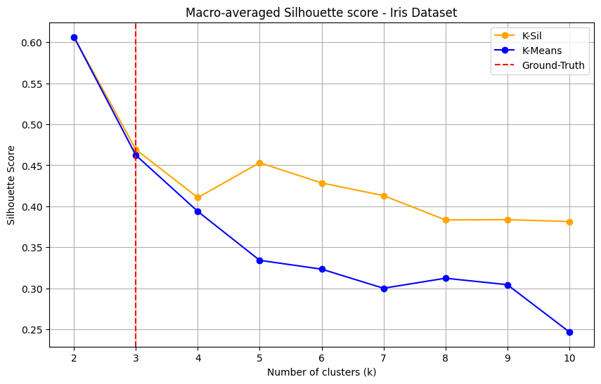
(a) Iris

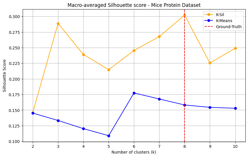
(b) Mice Protein

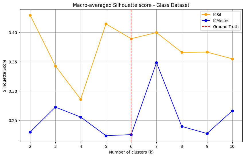
(c) Glass

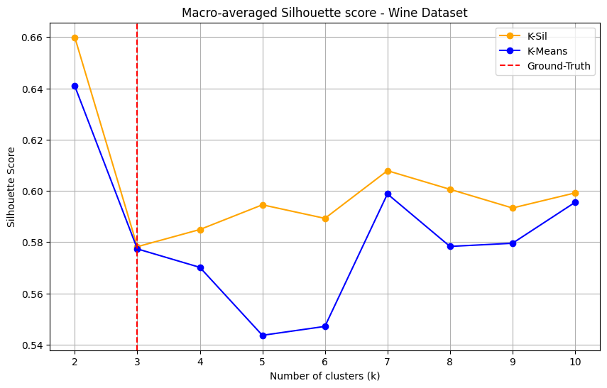
(d) Wine

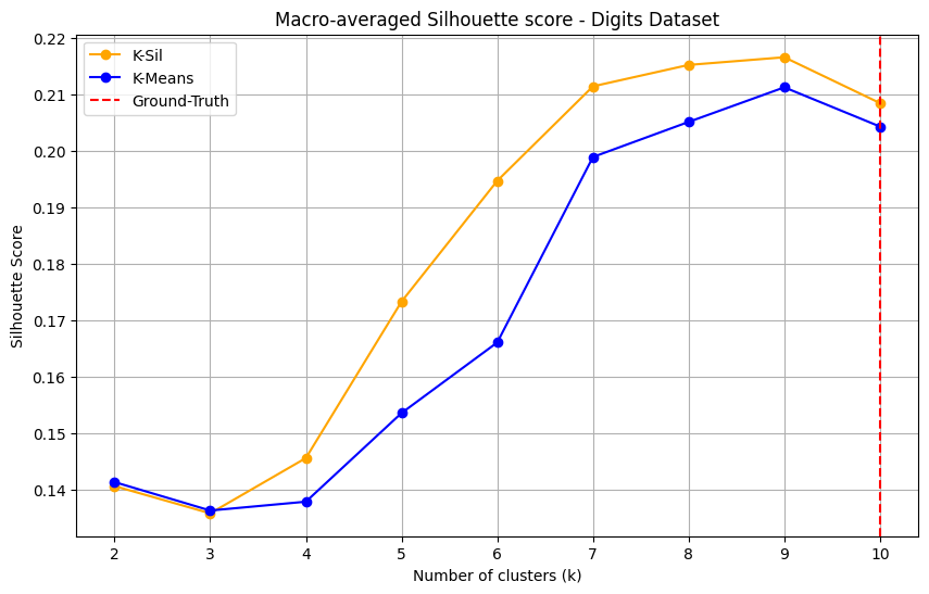
(e) Digits

(f) 20 Newsgroups Subset

Figure 6: Macro-averaged silhouette scores for K-Sil (orange) and standard k-means (blue) across the number of clusters $k\in\{2,\dots,10\}$ for real-world datasets (the ground-truth number of clusters $k_{GT}$ is indicated with a red dased line).
Both algorithms share the same initial centroids for each run. K-Sil is configured to prioritze $S_{\text{M}}$, utilizing the optimal weighting scheme with auto-tuned weight-sensitivity parameter for each $k$.

Table 7: Statistical comparison of silhouette score performance between K-Sil (prioritizing a convex combination of micro and macro-silhouette: $0.5S_{\text{m}}+0.5S_{\text{M}}$) and k-means. We report the average relative improvements (%) in $S_{\text{m}}$ and $S_{\text{M}}$ (along with the weighting scheme used, P: Power or E: Exponential) of K-Sil over k-means, across $k\in\{2,\dots,10\}$ and at the ground-truth number of clusters $k_{GT}$ for the statistically significant ($p<0.05$) results for each dataset (“-”for statistically insignificant improvements).

Dataset	Mean Relative Improvement on
	$\left(S_{\text{M}}\right)$		$\left(S_{\text{m}}\right)$
	Across $k$	On $k_{GT}$	Across $k$	On $k_{GT}$
S1	7.58% (P)	2.49% (P)	6.19% (P)	-
S2	46.51% (P)	42.55% (E)	35.71% (P)	29.01% (E)
S3	30.30% (P)	47.32% (E)	18.52% (P)	35.77% (E)
S4	17.21% (E)	29.01% (E)	5.34% (P)	8.63% (E)
Iris	13.17% (P)	1.60% (E)	7.78% (P)	-
Mice Protein	42.52% (E)	45.35% (P)	10.14% (P)	10.23% (P)
Glass	42.80% (E)	49.35% (E)	22.08% (P)	13.71% (P)
Wine	3.76% (E)	-	2.46% (E)	-
Digits	5.54% (P)	9.00% (P)	2.21% (P)	4.65% (P)
20 Newsgroups	168.02% (E)	241.92% (P)	-	-

References

- \bibcommenthead
- Jain et al. [1999] Jain, A.K., Murty, M.N., Flynn, P.J.: Data clustering: A review. ACM Computing Surveys 31(3), 264–323 (1999)
- MacQueen [1967] MacQueen, J.B.: Some methods for classification and analysis of multivariate observations. In: Proceedings of the 5th Berkeley Symposium on Mathematical Statistics and Probability, pp. 281–297 (1967)
- Pavlopoulos et al. [2025] Pavlopoulos, J., Vardakas, G., Likas, A.: Revisiting silhouette aggregation. In: Discovery Science, pp. 354–368. Springer, Cham (2025)
- Xu and Wunsch [2005] Xu, R., Wunsch, D.: Survey of clustering algorithms. IEEE Transactions on Neural Networks 16(3), 645–678 (2005)
- Rousseeuw [1987] Rousseeuw, P.J.: Silhouettes: A graphical aid to the interpretation and validation of cluster analysis. Journal of Computational and Applied Mathematics 20, 53–65 (1987)
- Dudek [2020] Dudek, A.: Silhouette index as clustering evaluation tool. In: Classification and Data Analysis: Theory and Applications 28, pp. 19–33 (2020). Springer
- Ester et al. [1996] Ester, M., Kriegel, H.-P., Sander, J., Xu, X.: A density-based algorithm for discovering clusters in large spatial databases with noise. In: Proceedings of the 2nd International Conference on Knowledge Discovery and Data Mining (KDD), pp. 226–231 (1996)
- Müllner [2011] Müllner, D.: Modern hierarchical, agglomerative clustering algorithms. arXiv preprint arXiv:1109.2378 (2011)
- Reynolds [2009] Reynolds, D.A.: Gaussian mixture models. Encyclopedia of Biometrics, 659–663 (2009)
- Ng et al. [2002] Ng, A.Y., Jordan, M.I., Weiss, Y.: On spectral clustering: Analysis and an algorithm. In: Advances in Neural Information Processing Systems (NeurIPS), vol. 14 (2002)
- Arthur and Vassilvitskii [2007] Arthur, D., Vassilvitskii, S.: K-means++ the advantages of careful seeding. In: Proceedings of the Eighteenth Annual ACM-SIAM Symposium on Discrete Algorithms, pp. 1027–1035 (2007)
- Bachem et al. [2016] Bachem, O., Lucic, M., Krause, A.: Fast and provably good seedings for k-means. In: Advances in Neural Information Processing Systems (NeurIPS), pp. 55–63 (2016)
- Krishna and Murty [1999] Krishna, K., Murty, M.: Genetic k-means algorithm. IEEE transactions on systems, man, and cybernetics. Part B, Cybernetics : a publication of the IEEE Systems, Man, and Cybernetics Society 29, 433–9 (1999)
- Likas et al. [2003] Likas, A., Vlassis, N., Verbeek, J.J.: The global k-means clustering algorithm. Pattern recognition 36(2), 451–461 (2003)
- Vardakas and Likas [2022] Vardakas, G., Likas, A.: Global -means: an effective relaxation of the global -means clustering algorithm. arXiv preprint arXiv:2211.12271 (2022)
- Sinaga and Yang [2020] Sinaga, K.P., Yang, M.-S.: Unsupervised k-means clustering algorithm. IEEE Access 8, 80716–80727 (2020)
- Huang et al. [2005] Huang, J.Z., Ng, M.K., Rong, H., Li, Z.: Automated variable weighting in k-means type clustering. IEEE Transactions on Pattern Analysis and Machine Intelligence 27(5), 657–668 (2005)
- Jing et al. [2007] Jing, L., Ng, M.K., Huang, J.Z.: An entropy weighting k-means algorithm for subspace clustering of high-dimensional sparse data. IEEE Transactions on Knowledge and Data Engineering 19(8), 1026–1041 (2007)
- Chan et al. [2004] Chan, E.Y., Ching, W.K., Ng, M.K., Huang, J.Z.: An optimization algorithm for clustering using weighted dissimilarity measures. Pattern Recognition 37(5), 943–952 (2004)
- Borgwardt et al. [2013] Borgwardt, S., Brieden, A., Gritzmann, P.: A balanced k-means algorithm for weighted point sets. ArXiv abs/1308.4004 (2013)
- Moggridge et al. [2020] Moggridge, P., Helian, N., Sun, Y., Lilley, M., Veneziano, V.: Instance weighted clustering: Local outlier factor and k-means. In: Iliadis, L., Angelov, P.P., Jayne, C., Pimenidis, E. (eds.) Proceedings of the 21st EANN (Engineering Applications of Neural Networks) 2020 Conference, pp. 435–446. Springer, Cham (2020)
- Arbelaitz et al. [2013] Arbelaitz, O., Gurrutxaga, I., Muguerza, J., Pérez, J.M., Perona, I.: An extensive comparative study of cluster validity indices. Pattern recognition 46(1), 243–256 (2013)
- Bombina et al. [2024] Bombina, P., Tally, D., Abrams, Z.B., Coombes, K.R.: Sillyputty: Improved clustering by optimizing the silhouette width. PLOS ONE 19(6), 1–17 (2024) https://doi.org/10.1371/journal.pone.0300358
- Lai et al. [2024] Lai, H., Huang, T., Lu, B., Zhang, S., Xiaog, R.: Silhouette coefficient-based weighting k-means algorithm. Neural Computing and Applications 37, 3061–3075 (2024)
- Batool and Hennig [2021] Batool, F., Hennig, C.: Clustering with the average silhouette width. Computational Statistics & Data Analysis 158, 107190 (2021)
- Dua and Graff [2017] Dua, D., Graff, C.: UCI Machine Learning Repository (2017). http://archive.ics.uci.edu/ml
- Pedregosa et al. [2011] Pedregosa, F., Varoquaux, G., Gramfort, A., Michel, V., Thirion, B., Grisel, O., Blondel, M., Prettenhofer, P., Weiss, R., Dubourg, V., Vanderplas, J., Passos, A., Cournapeau, D., Brucher, M., Perrot, M., Duchesnay, E.: Scikit-learn: Machine learning in Python. Journal of Machine Learning Research 12, 2825–2830 (2011)
- Rey and Neuhäuser [2011] Rey, D., Neuhäuser, M.: In: Lovric, M. (ed.) Wilcoxon-Signed-Rank Test, pp. 1658–1659. Springer, Berlin, Heidelberg (2011)