Tri-hypercharge versus tri-darkcharge

Abstract

We propose a minimal, ultraviolet-complete, and renormalizable extension of the Standard Model, in which the three generations of ordinary fermions are distinguished by family-dependent hypercharges, while three right-handed neutrinos are separated by a dark gauge symmetry that is trivial for all Standard Model fields. This setup yields a fully flipped inert doublet model. The model naturally realizes a hybrid scotoseesaw mechanism that accounts for the smallness of neutrino masses and the largeness of lepton mixing. Simultaneously, it explains the stability and relic abundance of dark matter through a residual dark parity and addresses the hierarchies of charged fermion masses and the suppression of quark mixing via higher-dimensional operators involving high-scale scalar singlets and vector-like fermions. We explore the phenomenological implications of the model and derive constraints from electroweak precision tests, collider searches, flavor-changing processes, and observations of dark matter.

I Introduction

Two major puzzles of the Standard Model (SM) are the discovery of neutrino oscillations and the existence of dark matter (DM). The SM predicts that neutrinos are massless and that flavor lepton numbers are conserved. However, experimental evidence for neutrino oscillations indicates that neutrinos have mass and that lepton flavor is violated [1, 2]. Furthermore, the SM particle content lacks any viable candidate for DM, which constitutes most of the mass in galaxies and galaxy clusters [3]. Another longstanding issue is the flavor problem: in the SM, all three fermion generations are identical under gauge symmetry. Consequently, the theory does not explain why there are precisely three fermion generations, nor the large hierarchies observed in charged fermion masses and mixings [4].

Various mechanisms have been proposed to explain the origin of neutrino masses. Among the most well-known are the seesaw mechanism [5, 6, 7, 8, 9, 10, 11, 12, 13, 14] and the scotogenic mechanism [15, 16, 17, 18, 19, 20, 21]. The smallness of neutrino masses may also be explained via a hybrid scenario in which both mechanisms contribute—the so-called scotoseesaw mechanism [22, 23, 24, 25, 26, 27, 28, 29, 30].

Regarding DM, the most straightforward approach involves introducing a real, neutral singlet scalar with a $\mathbb{Z}_{2}$ symmetry into the SM, where the added scalar is odd while all other fields are even [31]. Another familiar candidate is a neutral singlet fermion, often introduced to cancel gauge anomalies. The $\mathbb{Z}_{2}$ symmetry may be included ad hoc, or it may arise as a residual gauge symmetry [32, 33, 22].

The issue of fermion generation number can be approached using anomaly cancellation and QCD asymptotic freedom arguments [34, 35, 29], while charged fermion mass and mixing hierarchies may be explained through flavor-deconstructed models [36, 37, 38, 39, 40].

In this work, we construct a simple extension of the SM by “fully flipping” all fermion generations, including three right-handed neutrino singlets—the counterparts of the usual left-handed neutrinos—resulting in what we call the fully flipped inert doublet model. Concretely, we decompose the SM hypercharge symmetry into three generation-specific hypercharge symmetries,

$$U(1)_{Y}\to U(1)_{Y_{1}}\otimes U(1)_{Y_{2}}\otimes U(1)_{Y_{3}},$$ (1)

such that each ordinary fermion generation $a$ is charged only under the corresponding $U(1)_{Y_{a}}$, similar to the decomposition of lepton number into generation lepton numbers and in the spirit of recent works [41, 42]. Since the right-handed neutrino singlets carry zero hypercharge, they remain uncharged under all $U(1)_{Y_{a}}$. To distinguish them, we introduce an additional dark gauge symmetry, $U(1)_{\mathsf{D}}$, under which the right-handed neutrinos are charged, while all SM fermions are neutral (i.e., $\mathsf{D}=0$), as suggested in [43, 28, 30].

This setup leads to several interesting phenomenological consequences. First, if the SM Higgs doublet carries only the third-generation hypercharge, then only third-generation charged fermion masses are generated at the renormalizable level. The masses of the first- and second-generation charged fermions and the CKM mixings arise from higher-dimensional operators involving high-scale scalar singlets—flavons—which spontaneously break the three $U(1)_{Y_{a}}$ symmetries down to the SM hypercharge. This explains both the heaviness of the third generation and the smallness of the CKM mixing angles.

Second, assigning distinct dark charges $\delta_{1,2,3}$ to the right-handed neutrinos $\nu_{1,2,3R}$, anomaly cancellation for $[\mathrm{Gravity}]^{2}U(1)_{\mathsf{D}}$ and $U(1)_{\mathsf{D}}^{3}$ requires

$$\delta_{1}+\delta_{2}+\delta_{3}=0,\hskip 14.22636pt\delta^{3}_{1}+\delta^{3}_{2}+\delta^{3}_{3}=0.$$ (2)

A minimal nontrivial solution is $\delta_{1}=-\delta_{2}\neq 0$ and $\delta_{3}=0$. Normalizing $\delta_{1}=1$, we obtain $\mathsf{D}_{\nu{1,2,3R}}=1,-1,0$, consistent with [43, 28, 30].

Third, a residual dark parity emerges, $P_{\mathsf{D}}=(-1)^{\mathsf{D}}$, under which only $\nu_{1R}$ and $\nu_{2R}$ are odd ($P_{\mathsf{D}}=-1$), while all other fields are even. This structure naturally realizes a scotoseesaw mechanism: the seesaw contribution arises via $\nu_{3R}$, generating one light active neutrino, and the scotogenic contribution—mediated by $P_{\mathsf{D}}$-odd scalars and $\nu_{1,2R}$—generates a second light active neutrino.

Fourth, the model provides a viable DM candidate in the form of a dark Majorana neutrino, which is stabilized by the conserved dark parity and realized as the lightest $P_{\mathsf{D}}$-odd field. Finally, since each generation hypercharge is assigned to only one fermion generation, the number of $U(1)_{Y_{a}}$ symmetries equals the number of fermion generations, naturally explaining the origin of three generations.

The remainder of this paper is organized as follows. In Section II, we present the fundamental aspects of the model, including the gauge symmetry, particle content, residual symmetries, Yukawa interactions, and scalar potential. Section III is devoted to the scalar and gauge boson mass spectra. The fermion mass spectrum is analyzed in Section IV. Constraints from electroweak precision observables, collider searches, and flavor physics are discussed in Sections V, VI, and VII, respectively. DM phenomenology is examined in Section VIII, and our conclusions are summarized in Section IX.

II The fully flipped inert doublet model

As mentioned, this work considers a fully flipped inert doublet model where the scalar sector is enlarged by the inclusion of several gauge singlet scalars and an inert scalar doublet, while the fermionic content is added by charged vector like fermions and right-handed Majorana neutrinos, whose inclusion is necessary for the implementation of seesaw mechanisms that yields the small masses of the first and second generation of SM charged femions as well as tree level type I and one loop level radiative seesaw mechanisms that produces the tiny masses of the active neutrinos. The tree-level type I seesaw mechanism generates the atmospheric neutrino mass squared splittings, whereas the solar neutrino mass squared splittings arise from a radiative seesaw mechanism at one-loop level. Our theory is based on the gauge symmetry

$$SU(3)_{C}\otimes SU(2)_{L}\otimes U(1)_{Y_{1}}\otimes U(1)_{Y_{2}}\otimes U(1)_{Y_{3}}\otimes U(1)_{\mathsf{D}},$$ (3)

where the electric charge operator is embedded in that symmetry, so that it is given by

$$Q=T_{3}+Y_{1}+Y_{2}+Y_{3}.$$ (4)

In our proposed framework, the local $U(1)_{\mathsf{D}}$ gauge symmetry is assumed to be spontaneously broken down to a preserved discrete symmetry, referred to as dark parity $P_{\mathsf{D}}$. This residual symmetry plays a crucial role in ensuring the radiative origin of the solar neutrino mass-squared splitting, as it forbids tree-level contributions to certain neutrino masses. Moreover, the presence of $P_{\mathsf{D}}$ guarantees the stability of DM candidates in the model. The fermionic content of the model and their transformations properties under the extended gauge symmetry group $SU(3)_{C}\otimes SU(2)_{L}\otimes U(1)_{Y_{1}}\otimes U(1)_{Y_{2}}\otimes U(1)_{Y_{3}}\otimes U(1)_{\mathsf{D}}$, as well as under the residual dark parity $P_{\mathsf{D}}$ (defined as $P_{\mathsf{D}}=(-1)^{\mathsf{D}}$), are summarized in Table 1. Here, $q_{aL}=(u_{aL},d_{aL})^{T}$ and $l_{aL}=(\nu_{aL},e_{aL})^{T}$ denote the left-handed quark and lepton doublets for the three generations $a=1,2,3$.

Field	$SU(3)_{C}\otimes SU(2)_{L}$	$U(1)_{Y_{1}}$	$U(1)_{Y_{2}}$	$U(1)_{Y_{3}}$	$U(1)_{\mathsf{D}}$	$P_{\mathsf{D}}$
$q_{1L}$	$({\bf 3,2})$	$1/6$	$0$	$0$	$0$	$+$
$u_{1R}$	$({\bf 3,1})$	$2/3$	$0$	$0$	$0$	$+$
$d_{1R}$	$({\bf 3,1})$	$-1/3$	$0$	$0$	$0$	$+$
$l_{1L}$	$({\bf 1,2})$	$-1/2$	$0$	$0$	$0$	$+$
$e_{1R}$	$({\bf 1,1})$	$-1$	$0$	$0$	$0$	$+$
$q_{2L}$	$({\bf 3,2})$	$0$	$1/6$	$0$	$0$	$+$
$u_{2R}$	$({\bf 3,1})$	$0$	$2/3$	$0$	$0$	$+$
$d_{2R}$	$({\bf 3,1})$	$0$	$-1/3$	$0$	$0$	$+$
$l_{2L}$	$({\bf 1,2})$	$0$	$-1/2$	$0$	$0$	$+$
$e_{2R}$	$({\bf 1,1})$	$0$	$-1$	$0$	$0$	$+$
$q_{3L}$	$({\bf 3,2})$	$0$	$0$	$1/6$	$0$	$+$
$u_{3R}$	$({\bf 3,1})$	$0$	$0$	$2/3$	$0$	$+$
$d_{3R}$	$({\bf 3,1})$	$0$	$0$	$-1/3$	$0$	$+$
$l_{3L}$	$({\bf 1,2})$	$0$	$0$	$-1/2$	$0$	$+$
$e_{3R}$	$({\bf 1,1})$	$0$	$0$	$-1$	$0$	$+$
$\nu_{1R}$	$({\bf 1,1})$	$0$	$0$	$0$	$1$	$-$
$\nu_{2R}$	$({\bf 1,1})$	$0$	$0$	$0$	$-1$	$-$
$\nu_{3R}$	$({\bf 1,1})$	$0$	$0$	$0$	$0$	$+$

Table 1: Fermion fields and their quantum numbers. $P_{\mathsf{D}}$ is residual dark parity of $U(1)_{\mathsf{D}}$.

To break the extended gauge symmetry and generate the correct mass spectrum for the particles, we introduce several scalar fields in addition to the SM Higgs doublet $H=(H^{+}\,H^{0})^{T}$. First, a scalar singlet $\Phi$ is included to spontaneously break the $U(1)_{\mathsf{D}}$ symmetry down to the residual dark parity $P_{\mathsf{D}}$, while simultaneously generating Majorana masses for the right-handed neutrinos $\nu_{1,2R}$. Furthermore, four electrically neutral scalar singlets—$\varphi_{12}$, $\varphi_{23}$, $\phi_{12}$, and $\phi_{23}$—are introduced. These scalars, referred to as flavons, carry non-zero generation hypercharges (associated with $U(1)_{Y_{1,2,3}}$), arranged such that the total hypercharge remains zero. Their roles are twofold: (i) to break the generation hypercharge groups spontaneously down to the SM hypercharge $U(1)_{Y}$, and (ii) to explain the observed mass hierarchies and the small mixing angles in the quark sector. Each of these scalar fields acquires a vacuum expectation value (VEV), given by

$$\langle H\rangle = \frac{1}{\sqrt{2}}\begin{pmatrix}0\\ v\end{pmatrix},$$ (5)

$$\langle\Phi\rangle = \frac{1}{\sqrt{2}}\Lambda,\hskip 14.22636pt\langle\varphi_{23}\rangle\approx\langle\phi_{23}\rangle\approx\frac{1}{\sqrt{2}}v_{23},\hskip 14.22636pt\langle\varphi_{12}\rangle\approx\langle\phi_{12}\rangle\approx\frac{1}{\sqrt{2}}v_{12},$$ (6)

where $v=246$ GeV denotes the electroweak VEV. The other symmetry-breaking scales are assumed to lie well above the Fermi scale, i.e., $v_{12,23},\Lambda\gg v$. This hierarchy ensures that the couplings of the $126$ GeV SM-like Higgs boson remain very close to their SM values, preserving compatibility with current experimental constraints. To account for the observed mass hierarchies among the SM charged fermions and the smallness of quark mixing angles, we further assume a hierarchy among the flavon VEVs, specifically $v_{12}\gg v_{23}$. In addition to the aforementioned scalar fields, we introduce an inert scalar doublet $\eta=(\eta^{0}\,\eta^{-})^{T}$ and a complex scalar singlet $\rho$. Both of these are odd under the preserved dark parity $P_{\mathsf{D}}$ and, as such, must have vanishing VEVs to maintain $P_{\mathsf{D}}$ conservation. The presence of these inert scalars is crucial for realizing the scotogenic seesaw mechanism, in which the light neutrino mass matrix receives an additional radiative contribution at the one-loop level. The quantum numbers of all scalar fields under the gauge symmetry group in Eq. (3) and under $P_{\mathsf{D}}$ are summarized in Table 2. Notably, the fields $\phi_{12(23)}$ and $\varphi_{12(23)}^{*}$ transform identically under the full symmetry, i.e., $\phi_{12(23)}\sim\varphi_{12(23)}^{*3}$. Therefore, in principle, one could eliminate two scalar flavons (e.g., $\phi_{12}$ and $\phi_{23}$) and still retain the same symmetry-breaking pattern and phenomenology. This would yield a more economical scalar sector and a simpler scalar potential. However, such a minimal setup would complicate the ultraviolet completion of the model, especially if one aims to generate the effective Yukawa couplings via heavy vector-like fermions, rendering the ultraviolet theory less minimal and more involved.

Field	$SU(3)_{C}\otimes SU(2)_{L}$	$U(1)_{Y_{1}}$	$U(1)_{Y_{2}}$	$U(1)_{Y_{3}}$	$U(1)_{\mathsf{D}}$	$P_{\mathsf{D}}$
$H$	$({\bf 1,2})$	$0$	$0$	$1/2$	$0$	$+$
$\varphi_{23}$	$({\bf 1,1})$	$0$	$1/6$	$-1/6$	$0$	$+$
$\phi_{23}$	$({\bf 1,1})$	$0$	$-1/2$	$1/2$	$0$	$+$
$\varphi_{12}$	$({\bf 1,1})$	$1/6$	$-1/6$	$0$	$0$	$+$
$\phi_{12}$	$({\bf 1,1})$	$-1/2$	$1/2$	$0$	$0$	$+$
$\Phi$	$({\bf 1,1})$	$0$	$0$	$0$	$2$	$+$
$\eta$	$({\bf 1,2})$	$0$	$0$	$-1/2$	$-1$	$-$
$\rho$	$({\bf 1,1})$	$0$	$0$	$0$	$1$	$-$

Table 2: Scalar fields and their quantum numbers.

The spontaneous gauge symmetry breaking is implemented through the following way, $SU(3)_{C}\otimes SU(2)_{L}\otimes U(1)_{Y_{1}}\otimes U(1)_{Y_{2}}\otimes U(1)_{Y_{3}}\otimes U(1)_{\mathsf{D}}\stackrel{{\scriptstyle v_{12}}}{{\longrightarrow}}SU(3)_{C}\otimes SU(2)_{L}\otimes U(1)_{Y_{1}+Y_{2}}\otimes U(1)_{Y_{3}}\otimes U(1)_{\mathsf{D}}\stackrel{{\scriptstyle v_{23}}}{{\longrightarrow}}SU(3)_{C}\otimes SU(2)_{L}\otimes U(1)_{Y}\otimes U(1)_{\mathsf{D}}\stackrel{{\scriptstyle\Lambda}}{{\longrightarrow}}SU(3)_{C}\otimes SU(2)_{L}\otimes U(1)_{Y}\otimes R_{\mathsf{D}}\stackrel{{\scriptstyle v}}{{\longrightarrow}}SU(3)_{C}\otimes U(1)_{Q}\otimes R_{\mathsf{D}}$, in which we have assumed $\Lambda<v_{23}$ for the potential discovery of new physics at the LHC. Here $U(1)_{Q}$ is the electromagnetic symmetry and $R_{\mathsf{D}}$ is a residual symmetry of $U(1)_{\mathsf{D}}$ that conserves all the VEVs, $R_{\mathsf{D}}=(-1)^{k\mathsf{D}}$ for $k$ integer. This residual symmetry is automorphic to a discrete group, such as $R_{\mathsf{D}}\cong\mathbb{Z}_{2}=\{1,(-1)^{\mathsf{D}}\}$, for which $P_{\mathsf{D}}=(-1)^{\mathsf{D}}$ is called a residual dark parity of $U(1)_{\mathsf{D}}$. Under $P_{\mathsf{D}}$, the SM fields, $\nu_{3R}$, $\Phi$, $\varphi_{12,23}$, and $\phi_{12,23}$ transform trivially, i.e., $P_{\mathsf{D}}=1$, whereas $\nu_{1,2R}$, $\eta$, and $\rho$ transform nontrivially, i.e., $P_{\mathsf{D}}=-1$, as presented in Tables 1 and 2.

With the above scalar content, the scalar potential can be split in two parts, such as $V=V_{1}+V_{2}$, where $V_{1}$ contains terms involving $P_{\mathsf{D}}$-even scalars, $H,\Phi,\phi_{12,23}$, and $\varphi_{12,23}$, while $V_{2}$ contains terms of $P_{\mathsf{D}}$-odd scalars, $\eta$ and $\rho$, and mixing terms between these two kinds, i.e.,

$$V_{1} = \mu_{1}^{2}H^{\dagger}H+\lambda_{1}(H^{\dagger}H)^{2}+\mu_{2}^{2}\Phi^{*}\Phi+\lambda_{2}(\Phi^{*}\Phi)^{2}+\lambda_{3}(\Phi^{*}\Phi)(H^{\dagger}H)$$ (7)

$$+\mu_{3}^{2}\varphi_{23}^{*}\varphi_{23}+\mu_{4}^{2}\phi_{23}^{*}\phi_{23}+\lambda_{4}(\varphi_{23}^{*}\varphi_{23})^{2}+\lambda_{5}(\phi_{23}^{*}\phi_{23})^{2}+\lambda_{6}(\varphi_{23}^{*}\varphi_{23})(\phi_{23}^{*}\phi_{23})$$

$$+(\varphi_{23}^{*}\varphi_{23})(\lambda_{7}\Phi^{*}\Phi+\lambda_{8}H^{\dagger}H)+(\phi_{23}^{*}\phi_{23})(\lambda_{9}\Phi^{*}\Phi+\lambda_{10}H^{\dagger}H)$$

$$+\mu_{5}^{2}\varphi_{12}^{*}\varphi_{12}+\mu_{6}^{2}\phi_{12}^{*}\phi_{12}+\lambda_{11}(\varphi_{12}^{*}\varphi_{12})^{2}+\lambda_{12}(\phi_{12}^{*}\phi_{12})^{2}+\lambda_{13}(\varphi_{12}^{*}\varphi_{12})(\phi_{12}^{*}\phi_{12})$$

$$+(\varphi_{12}^{*}\varphi_{12})(\lambda_{14}\varphi_{23}^{*}\varphi_{23}+\lambda_{15}\phi_{23}^{*}\phi_{23}+\lambda_{16}\Phi^{*}\Phi+\lambda_{17}H^{\dagger}H)$$

$$+(\phi_{12}^{*}\phi_{12})(\lambda_{18}\varphi_{23}^{*}\varphi_{23}+\lambda_{19}\phi_{23}^{*}\phi_{23}+\lambda_{20}\Phi^{*}\Phi+\lambda_{21}H^{\dagger}H)$$

$$+(\lambda_{22}\varphi_{12}^{3}\phi_{12}+\lambda_{23}\varphi_{23}^{3}\phi_{23}+\mathrm{H.c.}),$$

$$V_{2} = \mu_{7}^{2}\eta^{\dagger}\eta+\mu_{8}^{2}\rho^{\dagger}\rho+\lambda_{24}(\eta^{\dagger}\eta)^{2}+\lambda_{25}(\rho^{\dagger}\rho)^{2}+\lambda_{26}(\eta^{\dagger}\eta)(\rho^{\dagger}\rho)$$ (8)

$$+(\eta^{\dagger}\eta)(\lambda_{27}\varphi_{12}^{*}\varphi_{12}+\lambda_{28}\phi_{12}^{*}\phi_{12}+\lambda_{29}\varphi_{23}^{*}\varphi_{23}+\lambda_{30}\phi_{23}^{*}\phi_{23}+\lambda_{31}\Phi^{*}\Phi+\lambda_{32}H^{\dagger}H)$$

$$+(\rho^{\dagger}\rho)(\lambda_{33}\varphi_{12}^{*}\varphi_{12}+\lambda_{34}\phi_{12}^{*}\phi_{12}+\lambda_{35}\varphi_{23}^{*}\varphi_{23}+\lambda_{36}\phi_{23}^{*}\phi_{23}+\lambda_{37}\Phi^{*}\Phi+\lambda_{38}H^{\dagger}H)$$

$$+\lambda_{39}(H^{\dagger}\eta)(\eta^{\dagger}H)+(\mu_{9}H\eta\rho+\mu_{10}\rho\rho\Phi^{*}+\mathrm{H.c.}),$$

where the parameters $\lambda$’s are dimensionless, while $\mu$’s have a mass dimension. Hermiticity of the scalar potential requires all parameters to be real, except for $\lambda_{22,23}$ and $\mu_{9,10}$, which may, in general, be complex. However, any complex phases in $\lambda_{22,23}$ and $\mu_{9,10}$ can be removed by suitable phase redefinitions of the scalar fields $\varphi_{12,23},\eta$, and $\rho$. Therefore, without loss of generality, we assume that all parameters in the scalar potential are real throughout our analysis. Furthermore, the quartic scalar couplings of the form $\varphi_{12}^{3}\phi_{12}$ and $\varphi_{23}^{3}\phi_{23}$ explicitly break the global $U(1)$ phase symmetries associated with the four flavon fields. This breaking ensures that no physical Nambu–Goldstone bosons appear in the spectrum, rendering the model free from unwanted massless scalar degrees of freedom.

Since the SM Higgs doublet carries only the third-generation hypercharge, only the third-generation Yukawa couplings are allowed at the renormalizable level. In contrast, the masses of the first and second generations of SM charged fermions, as well as the fermionic mixing angles, arise solely from nonrenormalizable Yukawa operators. Adopting an effective field theory (EFT) framework, we can express the relevant Yukawa interactions as follows:

$$\mathcal{L} \supset \begin{pmatrix}\bar{q}_{1L}&\bar{q}_{2L}&\bar{q}_{3L}\end{pmatrix}\begin{pmatrix}y^{u}_{11}\frac{\phi_{12}}{\Lambda_{12}}\frac{\phi_{23}}{\Lambda_{23}}&y^{u}_{12}\frac{\varphi_{12}}{\Lambda_{12}}\frac{\phi_{23}}{\Lambda_{23}}&y^{u}_{13}\frac{\varphi_{12}}{\Lambda_{12}}\frac{\varphi_{23}}{\Lambda_{23}}\\ y^{u}_{21}\frac{\phi_{12}}{\Lambda_{12}}\frac{\varphi^{*}_{12}}{\Lambda_{12}}\frac{\phi_{23}}{\Lambda_{23}}&y^{u}_{22}\frac{\phi_{23}}{\Lambda_{23}}&y^{u}_{23}\frac{\varphi_{23}}{\Lambda_{23}}\\ y^{u}_{31}\frac{\phi_{12}}{\Lambda_{12}}\frac{\varphi^{*}_{12}}{\Lambda_{12}}\frac{\phi_{23}}{\Lambda_{23}}\frac{\varphi^{*}_{23}}{\Lambda_{23}}&y^{u}_{32}\frac{\phi_{23}}{\Lambda_{23}}\frac{\varphi^{*}_{23}}{\Lambda_{23}}&y^{u}_{33}\end{pmatrix}\begin{pmatrix}u_{1R}\\ u_{2R}\\ u_{3R}\end{pmatrix}\tilde{H}$$ (9)

$$+\begin{pmatrix}\bar{q}_{1L}&\bar{q}_{2L}&\bar{q}_{3L}\end{pmatrix}\begin{pmatrix}y^{d}_{11}\frac{\phi^{*}_{12}}{\Lambda_{12}}\frac{\phi^{*}_{23}}{\Lambda_{23}}&y^{d}_{12}\frac{\varphi_{12}}{\Lambda_{12}}\frac{\phi^{*}_{23}}{\Lambda_{23}}&y^{d}_{13}\frac{\varphi_{12}}{\Lambda_{12}}\frac{\varphi_{23}}{\Lambda_{23}}\\ y^{d}_{21}\frac{\phi^{*}_{12}}{\Lambda_{12}}\frac{\varphi^{*}_{12}}{\Lambda_{12}}\frac{\phi^{*}_{23}}{\Lambda_{23}}&y^{d}_{22}\frac{\phi^{*}_{23}}{\Lambda_{23}}&y^{d}_{23}\frac{\varphi_{23}}{\Lambda_{23}}\\ y^{d}_{31}\frac{\varphi^{2}_{12}}{\Lambda^{2}_{12}}\frac{\varphi^{2}_{23}}{\Lambda^{2}_{23}}&y^{d}_{32}\frac{\varphi^{2}_{23}}{\Lambda^{2}_{23}}&y^{d}_{33}\end{pmatrix}\begin{pmatrix}d_{1R}\\ d_{2R}\\ d_{3R}\end{pmatrix}H$$

$$+\begin{pmatrix}\bar{l}_{1L}&\bar{l}_{2L}&\bar{l}_{3L}\end{pmatrix}\begin{pmatrix}y^{e}_{11}\frac{\phi^{*}_{12}}{\Lambda_{12}}\frac{\phi^{*}_{23}}{\Lambda_{23}}&y^{e}_{12}\frac{\phi_{12}}{\Lambda_{12}}\frac{\phi^{*}_{23}}{\Lambda_{23}}&y^{e}_{13}\frac{\phi_{12}}{\Lambda_{12}}\frac{\phi_{23}}{\Lambda_{23}}\\ y^{e}_{21}\frac{\phi^{*2}_{12}}{\Lambda^{2}_{12}}\frac{\phi^{*}_{23}}{\Lambda_{23}}&y^{e}_{22}\frac{\phi^{*}_{23}}{\Lambda_{23}}&y^{e}_{23}\frac{\phi_{23}}{\Lambda_{23}}\\ y^{e}_{31}\frac{\phi^{*2}_{12}}{\Lambda^{2}_{12}}\frac{\phi^{*2}_{23}}{\Lambda^{2}_{23}}&y^{e}_{32}\frac{\phi^{*2}_{23}}{\Lambda^{2}_{23}}&y^{e}_{33}\end{pmatrix}\begin{pmatrix}e_{1R}\\ e_{2R}\\ e_{3R}\end{pmatrix}H+\mathrm{H.c.},$$

where the coefficients $y$’s are dimensionless, $\Lambda_{12,23}$ denote the EFT cutoff scales, and $\tilde{H}=i\sigma_{2}H^{*}$ with $\sigma_{2}$ being the second Pauli matrix. To obtain a complete and renormalizable model, we include heavy fermionic messenger fields whose masses correspond to the heavy scales $\Lambda_{12,23}$. Indeed, we add to the fermionic spectrum three heavy vector-like $SU(2)_{L}$ singlet fermions for each charged sector, namely $u_{12,13,23}$, $d_{12,13,23}$ and $e_{12,13,23}$ for the up-type quark, down-type quark and charged lepton sectors, respectively. Their quantum number assignments under the model symmetries are presented in Table 3. Accordingly, we construct a set of renormalizable Yukawa interactions and bare mass terms for each charged fermion sector, given by:

$$\mathcal{L}_{\mathrm{Y}}^{u} = y_{1}^{u}\bar{q}_{1L}\tilde{H}u_{13R}+y_{2}^{u}\bar{u}_{13L}\phi_{23}u_{12R}+y_{3}^{u}\bar{u}_{12L}\phi_{12}u_{1R}+y_{4}^{u}\bar{u}_{13L}\varphi_{12}u_{23R}$$ (10)

$$+y_{5}^{u}\bar{u}_{23L}\phi_{23}u_{2R}+y_{6}^{u}\bar{u}_{23L}\varphi_{23}u_{3R}+y_{7}^{u}\bar{q}_{2L}\tilde{H}u_{23R}+y_{8}^{u}\bar{u}_{23L}\varphi_{12}^{*}u_{13R}$$

$$+y_{33}^{u}\bar{q}_{3L}\tilde{H}u_{3R}+m_{u_{12}}\bar{u}_{12L}u_{12R}+m_{u_{13}}\bar{u}_{13L}u_{13R}+m_{u_{23}}\bar{u}_{23L}u_{23R}+\mathrm{H.c.},$$

$$\mathcal{L}_{\mathrm{Y}}^{d} = \mathcal{L}_{\mathrm{Y}}^{u}(y^{u}\to y^{d},u\to d,\tilde{H}\to H,\phi\to\phi^{*},m_{u}\to m_{d}),$$ (11)

$$\mathcal{L}_{\mathrm{Y}}^{e} = \mathcal{L}_{\mathrm{Y}}^{u}(y^{u}\to y^{e},q\to l,u\to e,\tilde{H}\to H,\phi\to\phi^{*},\varphi\to\phi,m_{u}\to m_{e}),$$ (12)

where the coefficients $y$’s are dimensionless, whereas $m$’s have mass dimension.

Field	$SU(3)_{C}\otimes SU(2)_{L}$	$U(1)_{Y_{1}}$	$U(1)_{Y_{2}}$	$U(1)_{Y_{3}}$	$U(1)_{\mathsf{D}}$	$P_{\mathsf{D}}$
$u_{12}$	$({\bf 3,1})$	$1/6$	$1/2$	$0$	$0$	$+$
$u_{13}$	$({\bf 3,1})$	$1/6$	$0$	$1/2$	$0$	$+$
$u_{23}$	$({\bf 3,1})$	$0$	$1/6$	$1/2$	$0$	$+$
$d_{12}$	$({\bf 3,1})$	$1/6$	$-1/2$	$0$	$0$	$+$
$d_{13}$	$({\bf 3,1})$	$1/6$	$0$	$-1/2$	$0$	$+$
$d_{23}$	$({\bf 3,1})$	$0$	$1/6$	$-1/2$	$0$	$+$
$e_{12}$	$({\bf 1,1})$	$-1/2$	$-1/2$	$0$	$0$	$+$
$e_{13}$	$({\bf 1,1})$	$-1/2$	$0$	$-1/2$	$0$	$+$
$e_{23}$	$({\bf 1,1})$	$0$	$-1/2$	$-1/2$	$0$	$+$
$\nu_{13}$	$({\bf 1,1})$	$-1/2$	$0$	$1/2$	$0$	$+$
$\nu_{23}$	$({\bf 1,1})$	$0$	$-1/2$	$1/2$	$0$	$+$

Table 3: Vector-like fermions and their quantum numbers.

We also introduce two vector-like neutrinos, $\nu_{13,23}$, which are complete singlets under the SM gauge group. These fields enable the generation of light neutrino masses and mixings at tree level via the seesaw mechanism. Their quantum numbers under the gauge symmetry of Eq. (3) are listed in the last two rows of Table 3. The corresponding renormalizable Yukawa interactions relevant for neutrino mass generation are given by:

$$\mathcal{L}^{\nu}_{\mathrm{Y}} = y_{1}\bar{l}_{1L}\tilde{H}\nu_{13R}+y_{2}\bar{l}_{2L}\tilde{H}\nu_{23R}+y_{3}\bar{l}_{3L}\tilde{H}\nu_{3R}+x_{1}\bar{\nu}_{13L}\phi_{12}\nu_{23R}+x_{2}\bar{\nu}_{23L}\phi_{12}^{*}\nu_{13R}$$ (13)

$$+z_{1}\bar{\nu}_{23L}\phi_{23}\nu_{3R}+z_{2}\bar{\nu}_{3R}^{c}\phi_{23}^{*}\nu_{23R}-m_{\nu_{13}}\bar{\nu}_{13L}\nu_{13R}-m_{\nu_{23}}\bar{\nu}_{23L}\nu_{23R}-\frac{1}{2}M_{3}\bar{\nu}_{3R}^{c}\nu_{3R}$$

$$+\kappa\bar{l}_{3L}\eta\nu_{1R}+\frac{1}{2}f_{1}\bar{\nu}_{1R}^{c}\Phi^{*}\nu_{1R}+\frac{1}{2}f_{2}\bar{\nu}_{2R}^{c}\Phi\nu_{2R}-m_{12}\bar{\nu}_{1R}^{c}\nu_{2R}+\mathrm{H.c.},$$

where the coefficients $y_{1,2,3}$, $x_{1,2}$, $z_{1,2}$, $\kappa$ and $f_{1,2}$ are dimensionless, whereas $m$’s and $M_{3}$ have mass dimension.

III Gauge and scalar sectors

III.1 Gauge sector

In our model the covariant derivative takes the form $D_{\mu}=\partial_{\mu}+ig_{s}t_{p}G_{p\mu}+igT_{n}A_{n\mu}+ig_{1}Y_{1}B_{1\mu}+ig_{2}Y_{2}B_{2\mu}+ig_{3}Y_{3}B_{3\mu}+ig_{\mathsf{D}}\mathsf{D}C_{\mu}$, where $(g_{s},g,g_{1},g_{2},g_{3},g_{\mathsf{D}})$, $(t_{p},T_{n},Y_{1},Y_{2},Y_{3},\mathsf{D})$, and $(G_{p\mu},A_{n\mu},B_{1\mu},B_{2\mu},B_{3\mu},C_{\mu})$ are coupling constants, generators, and gauge bosons of the $(SU(3)_{C}$, $SU(2)_{L},U(1)_{Y_{1}},U(1)_{Y_{2}},U(1)_{Y_{3}},U(1)_{\mathsf{D}})$ groups, respectively. Substituting them into the scalar kinetic term $\sum_{S}(D^{\mu}\langle S\rangle)^{\dagger}(D_{\mu}\langle S\rangle)$ for $S=H,\Phi,\phi_{12,23},\varphi_{12,23}$, we find

$$\mathcal{L}\supset\frac{g^{2}v^{2}}{4}W^{\mu+}W_{\mu}^{-}+2g_{\mathsf{D}}^{2}\Lambda^{2}\mathsf{Z}^{\mu}\mathsf{Z}_{\mu}+\frac{1}{2}(A^{\mu}_{3}\,B^{\mu}_{3}\,B^{\mu}_{2}\,B^{\mu}_{1})M_{0}^{2}(A_{3\mu}\,B_{3\mu}\,B_{2\mu}\,B_{1\mu})^{T},$$ (14)

where $W^{\pm}_{\mu}=(A_{1\mu}\mp iA_{2\mu})/\sqrt{2}$ and $\mathsf{Z}_{\mu}\equiv C_{\mu}$ are physical fields by themselves, which are respectively identified with the SM charged and $U(1)_{\mathsf{D}}$ gauge bosons with their masses given by $m^{2}_{W}=g^{2}v^{2}/4$ and $m^{2}_{\mathsf{Z}}=4g^{2}_{\mathsf{D}}\Lambda^{2}$. For the last term, the mixing matrix

$$M_{0}^{2}=\begin{pmatrix}\frac{g^{2}v^{2}}{4}&-\frac{gg_{3}v^{2}}{4}&0&0\\ -\frac{gg_{3}v^{2}}{4}&\frac{g_{3}^{2}(10v_{23}^{2}+9v^{2})}{36}&-\frac{5g_{2}g_{3}v_{23}^{2}}{18}&0\\ 0&-\frac{5g_{2}g_{3}v_{23}^{2}}{18}&\frac{5g_{2}^{2}(v_{12}^{2}+v_{23}^{2})}{18}&-\frac{5g_{1}g_{2}v_{12}^{2}}{18}\\ 0&0&-\frac{5g_{1}g_{2}v_{12}^{2}}{18}&\frac{5g_{1}^{2}v_{12}^{2}}{18}\end{pmatrix}$$ (15)

always provides a zero eigenvalue with the corresponding eigenstate (photon field)

$$A_{\mu}=s_{W}A_{3}+c_{W}[s_{23}B_{3\mu}+c_{23}(s_{12}B_{2\mu}+c_{12}B_{1\mu})],$$ (16)

where the Weinberg angle $\theta_{W}$ and other mixing angles $\theta_{12,23}$ are given by

$$s_{W}=\frac{g_{Y}}{\sqrt{g_{Y}^{2}+g^{2}}},\hskip 14.22636pts_{12}=\frac{g_{1}}{\sqrt{g_{1}^{2}+g_{2}^{2}}},\hskip 14.22636pts_{23}=\frac{g_{12}}{\sqrt{g_{12}^{2}+g_{3}^{2}}},$$ (17)

for $g_{Y}=g_{12}g_{3}/\sqrt{g_{12}^{2}+g_{3}^{2}}$ and $g_{12}=g_{1}g_{2}/\sqrt{g_{1}^{2}+g_{2}^{2}}$. Here and throughout this work, we use a type of notation as $s_{x}\equiv\sin x$, $c_{x}\equiv\cos x$, and $t_{x}\equiv\tan x$ for any mixing angle either $\theta_{x}$ or $x$. Hence, we determine the SM $Z$ boson and two new neutral gauge bosons as follows

$$Z_{\mu} = c_{W}A_{3}-s_{W}[s_{23}B_{3\mu}+c_{23}(s_{12}B_{2\mu}+c_{12}B_{1\mu})],$$ (18)

$$Z_{1\mu} = c_{23}B_{3\mu}-s_{23}(s_{12}B_{2\mu}+c_{12}B_{1\mu}),$$ (19)

$$Z_{2\mu} = c_{12}B_{2\mu}-s_{12}B_{1\mu}.$$ (20)

In the $(A_{\mu},Z_{\mu},Z_{1\mu},Z_{2\mu})$ basis, the photon field is decoupled as a physical massless field, whereas the other states mix among themselves via the following squared mass matrix:

$$\mathcal{M}_{0}^{2}=\begin{pmatrix}\frac{g^{2}v^{2}}{4c_{W}^{2}}&-\frac{g_{3}g^{2}t_{W}v^{2}}{4g_{12}c_{W}}&0\\ -\frac{g_{3}g^{2}t_{W}v^{2}}{4g_{12}c_{W}}&\frac{g_{3}^{2}(9g^{4}t_{W}^{4}v^{2}+10g_{12}^{4}v_{23}^{2})}{36g^{2}g_{12}^{2}t_{W}^{2}}&-\frac{5g_{1}g_{2}g_{3}c_{12}^{2}v_{23}^{2}}{18gt_{W}}\\ 0&-\frac{5g_{1}g_{2}g_{3}c_{12}^{2}v_{23}^{2}}{18gt_{W}}&\frac{5[(g_{1}^{2}+g_{2}^{2})v_{12}^{2}+g_{2}^{2}c_{12}^{2}v_{23}^{2}]}{18}\end{pmatrix}.$$ (21)

This matrix can be approximately diagonalized by using the usual type I seesaw formula. Introducing a new basis as $(\mathcal{Z}_{\mu},\mathcal{Z}_{1\mu},\mathcal{Z}_{2\mu})$ for which the light $\mathcal{Z}_{\mu}$ boson is separated from the heavy bosons $\mathcal{Z}_{1\mu}$ and $\mathcal{Z}_{2\mu}$, we obtain $\mathcal{Z}_{\mu}\simeq Z_{\mu}-\varepsilon_{1}Z_{1\mu}-\varepsilon_{2}Z_{2\mu}$, $\mathcal{Z}_{1\mu}\simeq\varepsilon_{1}Z_{\mu}+Z_{1\mu}$, $\mathcal{Z}_{2\mu}\simeq\varepsilon_{2}Z_{\mu}+Z_{2\mu}$, and the mass of $\mathcal{Z}_{\mu}$ to be

$$m^{2}_{\mathcal{Z}}\simeq\frac{g^{2}v^{2}}{4c_{W}^{2}}\left(1+\frac{\varepsilon_{1}g_{3}s_{W}}{g_{12}}\right),$$ (22)

where the mixing parameters $\varepsilon_{1,2}$ are strongly suppressed by $(v/v_{23})^{2}$ and $(v/v_{12})^{2}$, respectively,

$$\varepsilon_{1}\simeq-\frac{9g^{4}t_{W}^{3}v^{2}}{10g_{12}^{3}g_{3}c_{W}v_{23}^{2}},\hskip 14.22636pt\varepsilon_{2}\simeq-\frac{9g^{3}c_{12}^{2}t_{W}^{2}v^{2}}{10g_{12}g_{1}g_{2}c_{W}v_{12}^{2}}.$$ (23)

The $\mathcal{Z}_{\mu}$ boson that has a mass at the weak scale is identical to the SM $Z$ boson.

The $\mathcal{Z}_{1\mu}$ and $\mathcal{Z}_{2\mu}$ bosons mix by themselves via a mass matrix which approximates the bottom-right $2\times 2$ submatrix of $\mathcal{M}_{0}^{2}$. Diagonalizing this mass matrix, we obtain the corresponding physical states,

$$Z_{23\mu}=c_{\zeta}\mathcal{Z}_{1\mu}-s_{\zeta}\mathcal{Z}_{2\mu},\hskip 14.22636ptZ_{12\mu}=s_{\zeta}\mathcal{Z}_{1\mu}+c_{\zeta}\mathcal{Z}_{2\mu},$$ (24)

with their respective masses

$$m^{2}_{Z_{23}}\simeq\frac{5g_{12}^{2}g_{3}^{2}v_{23}^{2}}{18g^{2}t_{W}^{2}},\hskip 14.22636ptm^{2}_{Z_{12}}\simeq\frac{5[(g_{1}^{2}+g_{2}^{2})v_{12}^{2}+g_{2}^{2}c_{12}^{2}v_{23}^{2}]}{18},$$ (25)

to be very heavy at the $v_{23}$ and $v_{12}$ scales, respectively. The $\zeta$ mixing angle is given by

$$t_{2\zeta}\simeq-\frac{2gg_{1}g_{2}g_{3}t_{W}c_{12}^{2}v_{23}^{2}}{g^{2}(g_{1}^{2}+g_{2}^{2})t_{W}^{2}v_{12}^{2}+(g^{2}g_{2}^{2}t_{W}^{2}c_{12}^{2}-g_{12}^{2}g_{3}^{2})v_{23}^{2}},$$ (26)

strongly suppressed by $(v_{23}/v_{12})^{2}$.

III.2 Scalar sector

To obtain the physical scalar spectrum, we first expand the scalar fields around their VEVs, such as

$$H = \begin{pmatrix}H^{+}\\ \frac{1}{\sqrt{2}}(v+S_{1}+iA_{1})\end{pmatrix},\hskip 14.22636pt\Phi=\frac{1}{\sqrt{2}}(\Lambda+S_{2}+iA_{2}),$$ (27)

$$\phi_{23} = \frac{1}{\sqrt{2}}(v_{23}+S_{3}+iA_{3}),\hskip 14.22636pt\varphi_{23}=\frac{1}{\sqrt{2}}(v_{23}+S_{4}+iA_{4}),$$ (28)

$$\phi_{12} = \frac{1}{\sqrt{2}}(v_{12}+S_{5}+iA_{5}),\hskip 14.22636pt\varphi_{12}=\frac{1}{\sqrt{2}}(v_{12}+S_{6}+iA_{6}),$$ (29)

$$\eta = \begin{pmatrix}\frac{1}{\sqrt{2}}(R_{\eta}+iI_{\eta})\\ \eta^{-}\end{pmatrix},\hskip 14.22636pt\rho=\frac{1}{\sqrt{2}}(R_{\rho}+iI_{\rho}),$$ (30)

and then substitute them into the scalar potential. Hence, the scalar potential minimization conditions are given by

$$2\mu_{1}^{2}+2\lambda_{1}v^{2}+\lambda_{3}\Lambda^{2}+(\lambda_{8}+\lambda_{10})v_{23}^{2}+(\lambda_{17}+\lambda_{21})v_{12}^{2} = 0,$$ (31)

$$2\mu_{2}^{2}+\lambda_{3}v^{2}+2\lambda_{2}\Lambda^{2}+(\lambda_{7}+\lambda_{9})v_{23}^{2}+(\lambda_{16}+\lambda_{20})v_{12}^{2} = 0,$$ (32)

$$2\mu_{3}^{2}+\lambda_{8}v^{2}+\lambda_{7}\Lambda^{2}+(2\lambda_{4}+\lambda_{6}+3\lambda_{23})v_{23}^{2}+(\lambda_{14}+\lambda_{18})v_{12}^{2} = 0,$$ (33)

$$2\mu_{4}^{2}+\lambda_{10}v^{2}+\lambda_{9}\Lambda^{2}+(2\lambda_{5}+\lambda_{6}+\lambda_{23})v_{23}^{2}+(\lambda_{15}+\lambda_{19})v_{12}^{2} = 0,$$ (34)

$$2\mu_{5}^{2}+\lambda_{17}v^{2}+\lambda_{16}\Lambda^{2}+(\lambda_{14}+\lambda_{15})v_{23}^{2}+(2\lambda_{11}+\lambda_{13}+3\lambda_{22})v_{12}^{2} = 0,$$ (35)

$$2\mu_{6}^{2}+\lambda_{21}v^{2}+\lambda_{20}\Lambda^{2}+(\lambda_{18}+\lambda_{19})v_{23}^{2}+(2\lambda_{12}+\lambda_{13}+\lambda_{22})v_{12}^{2} = 0.$$ (36)

For the CP-odd and $P_{\mathsf{D}}$-even scalar sector, $A_{1,2,3,4,5,6}$, we find two physical heavy mass eigenstates, $\mathcal{A}_{1}=-(A_{3}+3A_{4})/\sqrt{10}$ and $\mathcal{A}_{2}=-(A_{5}+3A_{6})/\sqrt{10}$, with corresponding masses, $m_{\mathcal{A}_{1}}=-5\lambda_{23}v_{23}^{2}$ and $m_{\mathcal{A}_{2}}=-5\lambda_{22}v_{12}^{2}$, then implying that the parameters $\lambda_{22,23}$ have be negative. Additionally, we also obtain four massless eigenstates, $G_{Z}=A_{1}$, $G_{\mathsf{Z}}=A_{2}$, $G_{Z_{1}}=(3A_{3}-A_{4})/\sqrt{10}$, and $G_{Z_{2}}=(3A_{5}-A_{6})/\sqrt{10}$, which are the Goldstone bosons eaten by the longitudinal components of the neutral gauge bosons, $Z$, $\mathsf{Z}$, $Z_{1}$, and $Z_{2}$, respectively.

For the CP-even and $P_{\mathsf{D}}$-even scalar sector, $S_{1,2,3,4,5,6}$, we find the following squared mass matrix

$$M^{2}_{S}=\begin{pmatrix}2\lambda_{1}v^{2}&\lambda_{3}\Lambda v&\lambda_{10}v_{23}v&\lambda_{8}v_{23}v&\lambda_{21}v_{12}v&\lambda_{17}v_{12}v\\ \lambda_{3}\Lambda v&2\lambda_{2}\Lambda^{2}&\lambda_{9}\Lambda v_{23}&\lambda_{7}\Lambda v_{23}&\lambda_{20}\Lambda v_{12}&\lambda_{16}\Lambda v_{12}\\ \lambda_{10}v_{23}v&\lambda_{9}\Lambda v_{23}&\frac{(4\lambda_{5}-\lambda_{23})v_{23}^{2}}{2}&\frac{(2\lambda_{6}+3\lambda_{23})v_{23}^{2}}{2}&\lambda_{19}v_{12}v_{23}&\lambda_{15}v_{12}v_{23}\\ \lambda_{8}v_{23}v&\lambda_{7}\Lambda v_{23}&\frac{(2\lambda_{6}+3\lambda_{23})v_{23}^{2}}{2}&\frac{(4\lambda_{4}+3\lambda_{23})v_{23}^{2}}{2}&\lambda_{18}v_{12}v_{23}&\lambda_{14}v_{12}v_{23}\\ \lambda_{21}v_{12}v&\lambda_{20}v_{12}\Lambda&\lambda_{19}v_{12}v_{23}&\lambda_{18}v_{12}v_{23}&\frac{(4\lambda_{12}-\lambda_{22})v_{12}^{2}}{2}&\frac{(2\lambda_{13}+3\lambda_{22})v_{12}^{2}}{2}\\ \lambda_{17}v_{12}v&\lambda_{16}v_{12}\Lambda&\lambda_{15}v_{12}v_{23}&\lambda_{14}v_{12}v_{23}&\frac{(2\lambda_{13}+3\lambda_{22})v_{12}^{2}}{2}&\frac{(4\lambda_{11}+3\lambda_{22})v_{12}^{2}}{2}\end{pmatrix}.$$ (37)

This matrix can be approximately diagonalized by using the hierarchies $v\ll\Lambda,v_{23}\ll v_{12}$. Indeed, neglecting the mixing between $S_{5,6}$ and $S_{1,2,3,4}$, the bottom-right $2\times 2$ submatrix provides two physical eigenstates $\mathcal{H}_{5,6}$ with their masses to be very heavy at the $v_{12}$ scale. For the rest, we use the seesaw approximation to separate the light state $S_{1}$ from the heavy states $S_{2,3,4}$. In a new basis denoted $(h,H_{2},H_{3},H_{4})$ such that $h$ is decoupled as a physical field, we get

$$h\simeq S_{1}-\epsilon_{2}S_{2}-\epsilon_{3}S_{3}-\epsilon_{4}S_{4}$$ (38)

with its mass to be

$$m^{2}_{h}\simeq 2\lambda_{1}v^{2}-[\epsilon_{2}\lambda_{3}\Lambda+(\epsilon_{3}\lambda_{10}+\epsilon_{4}\lambda_{8})v_{23}]v,$$ (39)

where the mixing parameters are suppressed as $\epsilon_{2}\sim v/\Lambda$ and $\epsilon_{3,4}\sim v/v_{23}$. The remaining states $H_{2}\simeq\epsilon_{2}S_{1}+S_{2}$, $H_{3}\simeq\epsilon_{3}S_{1}+S_{3}$, and $H_{4}\simeq\epsilon_{4}S_{1}+S_{4}$ mix by themselves via a $3\times 3$ submatrix, which provide three physical eigenstates $\mathsf{H}$ and $\mathcal{H}_{3,4}$ with their masses to be $m_{\mathsf{H}}$ heavy at the $\Lambda$ scale and $m_{\mathcal{H}_{3,4}}$ heavy at the $v_{23}$ scale. Hence, the $h$ boson with a mass in the weak scale is identified with the SM Higgs boson.

For the $P_{\mathsf{D}}$-odd scalars, $R_{1,2}$ and $I_{1,2}$, we find two mass matrices where they mix in each pair, namely

$$V \supset \frac{1}{2}\begin{pmatrix}R_{\eta}&R_{\rho}\end{pmatrix}\begin{pmatrix}M^{2}_{\eta}&-\frac{\mu_{9}v}{\sqrt{2}}\\ -\frac{\mu_{9}v}{\sqrt{2}}&M^{2}_{\rho}+\sqrt{2}\mu_{10}\Lambda\end{pmatrix}\begin{pmatrix}R_{\eta}\\ R_{\rho}\end{pmatrix}$$ (40)

$$+\frac{1}{2}\begin{pmatrix}I_{\eta}&I_{\rho}\end{pmatrix}\begin{pmatrix}M^{2}_{\eta}&\frac{\mu_{9}v}{\sqrt{2}}\\ \frac{\mu_{9}v}{\sqrt{2}}&M^{2}_{\rho}-\sqrt{2}\mu_{10}\Lambda\end{pmatrix}\begin{pmatrix}I_{\eta}\\ I_{\rho}\end{pmatrix},$$

where we have denoted $M^{2}_{\eta}=[2\mu^{2}_{7}+(\lambda_{27}+\lambda_{28})v_{12}^{2}+(\lambda_{29}+\lambda_{30})v_{23}^{2}+\lambda_{31}\Lambda^{2}+\lambda_{32}v^{2}]/2$ and $M^{2}_{\rho}=[2\mu^{2}_{8}+(\lambda_{33}+\lambda_{34})v_{12}^{2}+(\lambda_{35}+\lambda_{36})v_{23}^{2}+\lambda_{37}\Lambda^{2}+\lambda_{38}v^{2}]/2$. Defining two mixing angles $\theta_{R,I}$ via the tangent function as

$$t_{2R,2I}=\frac{\mp\sqrt{2}\mu_{9}v}{M^{2}_{\rho}-M^{2}_{\eta}\pm\sqrt{2}\mu_{10}\Lambda},$$ (41)

we obtain $P_{D}$-odd physical mass eigenstates $R_{1}=c_{R}R_{\eta}-s_{R}R_{\rho}$, $R_{2}=s_{R}R_{\eta}+c_{R}R_{\rho}$, $I_{1}=c_{I}I_{\eta}-s_{I}I_{\rho}$, and $I_{2}=s_{I}I_{\eta}+c_{I}I_{\rho}$, with respective masses,

$$m^{2}_{R_{1},I_{1}} \simeq M^{2}_{\eta}-\frac{\mu^{2}_{9}v^{2}/2}{M^{2}_{\rho}-M^{2}_{\eta}\pm\sqrt{2}\mu_{10}\Lambda},$$ (42)

$$m^{2}_{R_{2},I_{2}} \simeq M^{2}_{\rho}\pm\sqrt{2}\mu_{10}\Lambda+\frac{\mu^{2}_{9}v^{2}/2}{M^{2}_{\rho}-M^{2}_{\eta}\pm\sqrt{2}\mu_{10}\Lambda},$$ (43)

in which the approximations come from $|\theta_{R,I}|\ll 1$. Indeed, since the last two terms associated with $\mu_{9,10}$ in Eq. (8) are not suppressed by any existing symmetry, $\mu_{9,10}$ may be as large as the highest scale, i.e. $\mu_{9,10}\sim v_{12}$. In such case, we still have $|\theta_{R,I}|\sim v/v_{12}\ll 1$. Also, it is straightforward to derive $(m^{2}_{R_{1}}-m^{2}_{I_{1}})/m^{2}_{R_{1},I_{1}}\sim(v^{2}/v_{12}^{2})(\Lambda/v_{12})\ll 1$ and $(m^{2}_{R_{2}}-m^{2}_{I_{2}})/m^{2}_{R_{2},I_{2}}\sim\Lambda/v_{12}\ll 1$.

For the charged scalars, we directly obtain a massless eigenstate, $G_{W^{\pm}}=H^{\pm}$, which is the Goldstone boson eaten by the $W^{\pm}$ charged gauge boson. Additionally, the charged dark scalar $\eta^{\pm}$ is a physical field by itself with mass in the $v_{12}$ scale, i.e. $m^{2}_{\eta^{\pm}}=M^{2}_{\eta}+\lambda_{39}v^{2}/2$.

IV Fermion mass and mixing

IV.1 Charged fermion sector

The Feynman diagrams responsible for the mass generation and mixing of the up-type quarks are shown in Fig. 1. The corresponding diagrams for the down-type quarks (charged leptons) can be obtained by making the substitutions: $u\to d$, $\tilde{H}\to H$, and $\phi\to\phi^{*}$ ($q\to l$, $u\to e$, $\tilde{H}\to H$, $\phi\to\phi^{*}$, and $\varphi\to\phi$). After integrating out the heavy messenger fields, we obtain effective Yukawa interactions for the SM chiral charged fermions. Once the flavon fields acquire VEVs, these effective interactions generate the mass matrices for the SM charged fermions, which take the form:

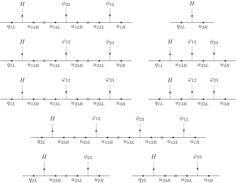
Figure 1: Diagrams relate to the generation of up-quark masses and mixing.

$$\mathcal{M}_{u} = \frac{v}{\sqrt{2}}\begin{pmatrix}\frac{y_{1}^{u}y_{2}^{u}y_{3}^{u}\langle\phi_{12}\rangle\langle\phi_{23}\rangle}{m_{u_{12}}m_{u_{13}}}&\frac{y_{1}^{u}y_{5}^{u}\langle\phi_{23}\rangle}{y_{8}^{u}\langle\varphi^{*}_{12}\rangle}+\frac{y_{1}^{u}y_{4}^{u}y_{5}^{u}\langle\varphi_{12}\rangle\langle\phi_{23}\rangle}{m_{u_{13}}m_{u_{23}}}&\frac{y_{1}^{u}y_{6}^{u}\langle\varphi_{23}\rangle}{y_{8}^{u}\langle\varphi^{*}_{12}\rangle}+\frac{y_{1}^{u}y_{4}^{u}y_{6}^{u}\langle\varphi_{12}\rangle\langle\varphi_{23}\rangle}{m_{u_{13}}m_{u_{23}}}\\ \frac{y_{2}^{u}y_{3}^{u}y_{7}^{u}y_{8}^{u}\langle\varphi_{12}^{*}\rangle\langle\phi_{12}\rangle\langle\phi_{23}\rangle}{m_{u_{12}}m_{u_{13}}m_{u_{23}}}&\frac{y_{5}^{u}y_{7}^{u}\langle\phi_{23}\rangle}{m_{u_{23}}}&\frac{y_{6}^{u}y_{7}^{u}\langle\varphi_{23}\rangle}{m_{u_{23}}}\\ 0&0&y_{33}^{u}\end{pmatrix},$$ (44)

$$\mathcal{M}_{d} = \frac{v}{\sqrt{2}}\begin{pmatrix}\frac{y_{1}^{d}y_{2}^{d}y_{3}^{d}\langle\phi^{*}_{12}\rangle\langle\phi^{*}_{23}\rangle}{m_{d_{12}}m_{d_{13}}}&\frac{y_{1}^{d}y_{5}^{d}\langle\phi^{*}_{23}\rangle}{y_{8}^{d}\langle\varphi^{*}_{12}\rangle}+\frac{y_{1}^{d}y_{4}^{d}y_{5}^{d}\langle\varphi_{12}\rangle\langle\phi^{*}_{23}\rangle}{m_{d_{13}}m_{d_{23}}}&\frac{y_{1}^{d}y_{6}^{d}\langle\varphi_{23}\rangle}{y_{8}^{d}\langle\varphi^{*}_{12}\rangle}+\frac{y_{1}^{d}y_{4}^{d}y_{6}^{d}\langle\varphi_{12}\rangle\langle\varphi_{23}\rangle}{m_{d_{13}}m_{d_{23}}}\\ \frac{y_{2}^{d}y_{3}^{d}y_{7}^{d}y_{8}^{d}\langle\varphi_{12}^{*}\rangle\langle\phi^{*}_{12}\rangle\langle\phi^{*}_{23}\rangle}{m_{d_{12}}m_{d_{13}}m_{d_{23}}}&\frac{y_{5}^{d}y_{7}^{d}\langle\phi^{*}_{23}\rangle}{m_{d_{23}}}&\frac{y_{6}^{d}y_{7}^{d}\langle\varphi_{23}\rangle}{m_{d_{23}}}\\ 0&0&y_{33}^{d}\end{pmatrix},$$ (45)

$$\mathcal{M}_{e} = \frac{v}{\sqrt{2}}\begin{pmatrix}\frac{y_{1}^{e}y_{2}^{e}y_{3}^{e}\langle\phi^{*}_{12}\rangle\langle\phi^{*}_{23}\rangle}{m_{e_{12}}m_{e_{13}}}&\frac{y_{1}^{e}y_{5}^{e}\langle\phi^{*}_{23}\rangle}{y_{8}^{e}\langle\phi^{*}_{12}\rangle}+\frac{y_{1}^{e}y_{4}^{e}y_{5}^{e}\langle\phi_{12}\rangle\langle\phi^{*}_{23}\rangle}{m_{e_{13}}m_{e_{23}}}&\frac{y_{1}^{e}y_{6}^{e}\langle\phi_{23}\rangle}{y_{8}^{u}\langle\phi^{*}_{12}\rangle}+\frac{y_{1}^{e}y_{4}^{e}y_{6}^{e}\langle\phi_{12}\rangle\langle\phi_{23}\rangle}{m_{e_{13}}m_{e_{23}}}\\ \frac{y_{2}^{e}y_{3}^{e}y_{7}^{e}y_{8}^{e}\langle\phi_{12}^{*}\rangle\langle\phi^{*}_{12}\rangle\langle\phi^{*}_{23}\rangle}{m_{e_{12}}m_{e_{13}}m_{e_{23}}}&\frac{y_{5}^{e}y_{7}^{e}\langle\phi^{*}_{23}\rangle}{m_{e_{23}}}&\frac{y_{6}^{e}y_{7}^{e}\langle\phi_{23}\rangle}{m_{e_{23}}}\\ 0&0&y_{33}^{e}\end{pmatrix}.$$ (46)

It is precisely that the $(3,1)$ and $(3,2)$ elements are not be generated at tree-level, while other components are naturally small with respect to the $(3,3)$ element, as suppressed by the ratios of flavon VEVs over messenger masses as well as the assumption $v_{23}\ll v_{12}$. The large amount of parametric freedom allows us to parametrize the low-energy SM charged fermion mass matrices as follows:

$$\mathcal{M}_{u} = \frac{v}{\sqrt{2}}\begin{pmatrix}y^{u}_{11}\lambda^{7}&y^{u}_{12}\lambda^{6}&y^{u}_{13}\lambda^{5}\\ y^{u}_{21}\lambda^{8}&y^{u}_{22}\lambda^{4}&y^{u}_{23}\lambda^{3}\\ 0&0&y_{33}^{u}\end{pmatrix},\hskip 14.22636pt\mathcal{M}_{d}=\frac{v}{\sqrt{2}}\begin{pmatrix}y_{11}^{d}\lambda^{7}&y_{12}^{d}\lambda^{7}&y_{13}^{d}\lambda^{6}\\ y_{21}^{d}\lambda^{9}&y_{22}^{d}\lambda^{5}&y_{23}^{d}\lambda^{4}\\ 0&0&y_{33}^{d}\end{pmatrix},$$ (47)

$$\mathcal{M}_{e} = \frac{v}{\sqrt{2}}\begin{pmatrix}y_{11}^{e}\lambda^{6}&y_{12}^{e}\lambda^{6}&y_{13}^{e}\lambda^{6}\\ y_{21}^{e}\lambda^{7}&y_{22}^{e}\lambda^{5}&y_{23}^{e}\lambda^{5}\\ 0&0&y_{33}^{e}\end{pmatrix},$$ (48)

where the coefficients $y$’s are dimensionless and $\lambda$ is the Wolfenstein parameter, $\lambda=0.22501(68)$ [44].

By applying biunitary transformations, we can diagonalize the $\mathcal{M}_{u,d,e}$ mass matrices separately, and then get the realistic masses of the up quarks $u,c,t$, the down quarks $d,s,b$, as well as the charged leptons $e,\mu,\tau$, such as

$$V_{u_{L}}^{\dagger}\mathcal{M}_{u}V_{u_{R}} = \text{diag}(m_{u},m_{c},m_{t}),$$ (49)

$$V_{d_{L}}^{\dagger}\mathcal{M}_{d}V_{d_{R}} = \text{diag}(m_{d},m_{s},m_{b}),$$ (50)

$$V_{e_{L}}^{\dagger}\mathcal{M}_{e}V_{e_{R}} = \text{diag}(m_{e},m_{\mu},m_{\tau}),$$ (51)

where $V_{u_{L,R}}$, $V_{d_{L,R}}$ and $V_{e_{L,R}}$ are unitary matrices, linking gauge states, $u_{a}=(u_{1},u_{2},u_{3})$, $d_{a}=(d_{1},d_{2},d_{3})$, $e_{a}=(e_{1},e_{2},e_{3})$, to mass eigenstates, $u_{i}=(u,c,t)$, $d_{i}=(d,s,b)$, $e_{i}=(e,\mu,\tau)$, respectively, namely

$$u_{aL,R}=[V_{u_{L,R}}]_{ai}u_{iL,R},\hskip 14.22636ptd_{aL,R}=[V_{d_{L,R}}]_{ai}d_{iL,R},\hskip 14.22636pte_{aL,R}=[V_{e_{L,R}}]_{ai}e_{iL,R}.$$ (52)

Here, $a(i)=1,2,3$ labels mass (gauge) eigenstates. Then, the Cabibbo-Kobayashi-Maskawa (CKM) matrix is defined by $V=V_{u_{L}}^{\dagger}V_{d_{L}}$.

IV.2 Neutral fermion sector

From the terms of the first two rows of Eq. (13), we obtain a full neutrino mass matrix in the basis $(\nu_{aL},\nu_{13L},\nu_{23L},\nu_{13R}^{c},\nu_{23R}^{c},\nu_{3R}^{c})$, which has the form

$$\begin{pmatrix}0&M_{D}\\ M_{D}^{T}&M_{M}\end{pmatrix},$$ (53)

where the submatrices are given by

$$M_{D} = -\frac{v}{\sqrt{2}}\begin{pmatrix}0&0&y_{1}&0&0\\ 0&0&0&y_{2}&0\\ 0&0&0&0&y_{3}\end{pmatrix},$$ (54)

$$M_{M} = -\frac{1}{\sqrt{2}}\begin{pmatrix}0&0&m_{\nu_{13}}&x_{1}v_{12}&0\\ 0&0&x_{2}v_{12}&m_{\nu_{23}}&z_{1}v_{23}\\ m_{\nu_{13}}&x_{2}v_{12}&0&0&0\\ x_{1}v_{12}&m_{\nu_{23}}&0&0&z_{2}v_{23}\\ 0&z_{1}v_{23}&0&z_{2}v_{23}&\sqrt{2}M_{3}\end{pmatrix}.$$ (55)

With the aid of $M_{3},m_{\nu_{13,23}},v_{12,23}\gg v$ thus $M_{M}\gg M_{D}$, we can apply the seesaw formula to extract a $3\times 3$ mass submatrix for the light neutrino part, i.e., $M_{\nu}^{\mathrm{tree}}\simeq-M_{D}M_{M}^{-1}M_{D}^{T}$. Further, assuming $M_{3}\gg m_{\nu_{13}}\simeq m_{\nu_{23}}\simeq v_{12}$ and taking $z_{1}=z_{2}=1$, we find

$$M_{\nu}^{\mathrm{tree}}\simeq\frac{v^{2}}{2M_{3}}\begin{pmatrix}\frac{y_{1}^{2}x_{1}^{2}v_{23}^{2}}{(x_{1}x_{2}-1)^{2}v_{12}^{2}}&-\frac{y_{1}y_{2}x_{1}v_{23}^{2}}{(x_{1}x_{2}-1)^{2}v_{12}^{2}}&\frac{y_{1}y_{3}x_{1}v_{23}}{(x_{1}x_{2}-1)v_{12}}\\ -\frac{y_{1}y_{2}x_{1}v_{23}^{2}}{(x_{1}x_{2}-1)^{2}v_{12}^{2}}&\frac{y_{2}^{2}v_{23}^{2}}{(x_{1}x_{2}-1)^{2}v_{12}^{2}}&-\frac{y_{2}y_{3}v_{23}}{(x_{1}x_{2}-1)v_{12}}\\ \frac{y_{1}y_{3}x_{1}v_{23}}{(x_{1}x_{2}-1)v_{12}}&-\frac{y_{2}y_{3}v_{23}}{(x_{1}x_{2}-1)v_{12}}&y_{3}^{2}\end{pmatrix}.$$ (56)

Notably, this texture can account for the large neutrino mixing angles while keeping all relevant Yukawa couplings of order $\mathcal{O}(1)$, as naturally expected in flavor models. It also reproduces the observed neutrino mass scale, $m_{\nu}\sim 0.1$ eV, with a heavy mass scale, $M_{3}\sim 10^{11}$ TeV. Importantly, this outcome does not require fine-tuning of small Yukawa couplings, nor does it demand the gauge symmetry-breaking scales $v_{12}$ and $v_{23}$ to be huge. Consequently, these scales can generally reside within the multi-TeV range.

It is worth emphasizing that the neutrino mass matrix $M_{\nu}^{\mathrm{tree}}$ generated at tree level via the seesaw mechanism has rank 1. As a result, it yields only one massive active neutrino and two massless ones, which is incompatible with current neutrino oscillation data [4]. Fortunately, the interactions of the third row of Eq. (13), together with the last two scalar couplings in Eq. (8), induce a one-loop radiative correction to the neutrino mass matrix, as illustrated in Fig. 2. In the mass eigenstate basis, the interactions relevant to this radiative contribution are given by:

$$\mathcal{L}\supset\frac{\kappa V_{1\alpha}}{\sqrt{2}}\bar{\nu}_{3L}(c_{R}R_{1}+s_{R}R_{2}+ic_{I}I_{1}+is_{I}I_{2})N_{\alpha R}+\mathrm{H.c.},$$ (57)

where $V$ is a $2\times 2$ rotation matrix,

$$V=\begin{pmatrix}c_{\xi}&s_{\xi}\\ -s_{\xi}&c_{\xi}\end{pmatrix},$$ (58)

relating $\nu_{1,2R}$ to their two mass eigenstates $N_{\alpha R}$ for $\alpha=1,2$. The respective mass eigenvalues and mixing angle are given by $M_{1,2}=\frac{1}{2}[m_{\nu_{1R}}+m_{\nu_{2R}}\mp\sqrt{(m_{\nu_{1R}}-m_{\nu_{2R}})^{2}+4m_{12}^{2}}]$ and $t_{2\xi}=2m_{12}/(m_{\nu_{1R}}-m_{\nu_{2R}})$ with $m_{\nu_{1,2R}}=-f_{1,2}\Lambda/\sqrt{2}$. Hence, the radiative contribution is defined by

$$M_{\nu}^{\mathrm{rad}}=\frac{(\kappa V_{1\alpha})^{2}M_{\alpha}}{32\pi^{2}}\left(\frac{c^{2}_{R}m^{2}_{R_{1}}\ln\frac{M_{\alpha}^{2}}{m^{2}_{R_{1}}}}{M_{\alpha}^{2}-m^{2}_{R_{1}}}-\frac{c^{2}_{I}m^{2}_{I_{1}}\ln\frac{M_{\alpha}^{2}}{m^{2}_{I_{1}}}}{M_{\alpha}^{2}-m^{2}_{I_{1}}}+\frac{s^{2}_{R}m^{2}_{R_{2}}\ln\frac{M_{\alpha}^{2}}{m^{2}_{R_{2}}}}{M_{\alpha}^{2}-m^{2}_{R_{2}}}-\frac{s^{2}_{I}m^{2}_{I_{2}}\ln\frac{M_{\alpha}^{2}}{m^{2}_{I_{2}}}}{M_{\alpha}^{2}-m^{2}_{I_{2}}}\right).$$ (59)

Because the dark scalar mixings and mass splittings are significantly suppressed, i.e., $|\theta_{R,I}|\sim v/v_{12}\ll 1$, $(m^{2}_{R_{1}}-m^{2}_{I_{1}})/m^{2}_{R_{1},I_{1}}\sim(v^{2}/v_{12}^{2})(\Lambda/v_{12})\ll 1$, $(m^{2}_{R_{2}}-m^{2}_{I_{2}})/m^{2}_{R_{2},I_{2}}\sim\Lambda/v_{12}\ll 1$, and the physical $P_{\mathsf{D}}$-odd right-handed neutrinos are much lighter than the dark neutral scalars, i.e., $M_{\alpha}/m_{R_{1},R_{2},I_{1},I_{2}}\sim\Lambda/v_{12}\ll 1$, the radiative contribution is proportional to $(\kappa^{2}V_{1\alpha}^{2}/32\pi^{2})(v^{2}/v_{12})(\Lambda^{2}/v_{12}^{2})\sim 0.1$ eV, taking $\kappa\sim\mathcal{O}(1)$, $\Lambda\sim\mathcal{O}(1)$ TeV, and $v_{12}\sim\mathcal{O}(10^{3})$ TeV, as expected.

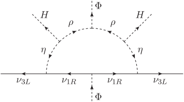
Figure 2: Scotogenic neutrino mass generation governed by residual dark parity.

Finally, it is worth noting that the total neutrino mass matrix, given by $M_{\nu}^{\mathrm{tot}}=M_{\nu}^{\mathrm{tree}}+M_{\nu}^{\mathrm{rad}}$, has rank 2. This structure yields two massive active neutrinos and one massless neutrino, which is sufficient to accommodate current neutrino oscillation data [4]. This outcome is reminiscent of what one obtains in a minimal type-I seesaw/scotogenic/scotoseesaw extension of the SM with only two right-handed neutrinos [12, 45, 46, 19, 23]. The total neutrino mass matrix can be diagonalized via a unitary transformation: $V_{\nu_{L}}^{T}M_{\nu}^{\mathrm{tot}}V_{\nu_{L}}=\text{diag}(0,m_{2},m_{3})$, where $m_{2,3}$ are the physical neutrino masses, and $V_{\nu_{L}}$ is a unitary matrix that relates the gauge basis neutrino states $\nu_{aL}=(\nu_{1L},\nu_{2L},\nu_{3L})^{T}$ to the physical flavor eigenstates $\nu_{iL}=(\nu_{eL},\nu_{\mu L},\nu_{\tau L})^{T}$ via $\nu_{aL}=[V_{\nu_{L}}]_{ai}\nu_{iL}$. Consequently, the Pontecorvo–Maki–Nakagawa–Sakata (PMNS) matrix, which governs neutrino mixing in charged-current interactions, is given by $V_{\text{PMNS}}=V_{\nu_{L}}^{\dagger}V_{e_{L}}$, where $V_{e_{L}}$ is the unitary matrix that diagonalizes the charged lepton mass matrix.

IV.3 Number analysis of fermion spectrum

Observable	Experimental value	Model value
$m_{u}$ [MeV]	$1.24\pm 0.22$	$1.24901$
$m_{c}$ [GeV]	$0.62\pm 0.02$	$0.61993$
$m_{t}$ [GeV]	$172.9\pm 0.4$	$172.901$
$m_{d}$ [MeV]	$2.69\pm 0.19$	$2.68948$
$m_{s}$ [MeV]	$53.5\pm 4.6$	$53.4558$
$m_{b}$ [GeV]	$2.86\pm 0.03$	$2.86009$
$\sin\theta^{(q)}_{12}$	$0.22501\pm 0.00068$	$0.225011$
$\sin\theta^{(q)}_{23}$	$0.04183_{-0.00069}^{+0.00079}$	$0.041829$
$\sin\theta^{(q)}_{13}$	$0.003732^{+0.000090}_{-0.000085}$	$0.003732$
$J_{q}$	$\left(3.12^{+0.13}_{-0.12}\right)\times 10^{-5}$	$3.11993\times 10^{-5}$

Table 4: Experimental values of the SM quark masses [47] and CKM parameters [4] along with the model values obtained for the best fit solution corresponding to $\chi^{2}\simeq 2\times 10^{-4}$.

To determine the best-fit parameters that reproduce the observed fermion masses and mixing, we minimize the $\chi^{2}$ function, defined as

$$\chi^{2}=\sum_{i}\left(\frac{O_{i}^{\text{calc}}-O_{i}^{\text{exp}}}{\Delta O_{i}}\right)^{2},$$ (60)

where $O_{i}^{\text{calc}}$ and $O_{i}^{\text{exp}}$ denote the model prediction and the experimental central value of the $i$-th observable, respectively, and $\Delta O_{i}$ represents its associated uncertainty. In the quark sector, the summation runs over the six quark masses, the CKM mixing angles, and the Jarlskog invariant, with the uncertainties $\Delta O_{i}$ taken as the $3\sigma$ experimental errors. As summarized in Table 4, our model successfully accommodates the observed quark mass spectrum, CKM mixing angles, and Jarlskog invariant, taking

$$y_{11}^{u} \simeq -0.274808,\hskip 14.22636pty_{12}^{u}\simeq-2.8602,\hskip 14.22636pty_{13}^{u}\simeq 6.23966,\hskip 14.22636pty_{21}^{u}\simeq 1.17024,$$ (61)

$$y_{22}^{u} \simeq 1.38277,\hskip 14.22636pty_{23}^{u}\simeq 0.283248,\hskip 14.22636pty_{33}^{u}\simeq 0.993968,\hskip 14.22636pt\text{arg}~(y_{13}^{u})\simeq 108.115^{\circ},$$ (62)

$$y_{11}^{d} \simeq -0.52976,\hskip 14.22636pty_{12}^{d}\simeq-1.28349,\hskip 14.22636pty_{13}^{d}\simeq 0.883176,\hskip 14.22636pty_{21}^{d}\simeq 0.598669,$$ (63)

$$y_{22}^{d} \simeq -0.52933,\hskip 14.22636pty_{23}^{d}\simeq-0.286541,\hskip 14.22636pty_{33}^{d}\simeq-0.0164254.$$ (64)

These results indicate that the Yukawa couplings $y^{u,d}_{1,2,\cdots,8}$ are all of order $\mathcal{O}(1)$. In the analysis above, all parameters are assumed to be real, except for $y_{13}^{u}$, which is taken to be complex and is solely responsible for generating the CP-violating phase in the quark sector. Furthermore, the correlation between the quark mixing angles and the Jarlskog invariant is illustrated in Fig. 3. The figure demonstrates that the Jarlskog invariant exhibits strong sensitivity to variations in the mixing angles $\theta_{13}^{(q)}$ and $\theta_{23}^{(q)}$, while being largely insensitive to changes in $\theta_{12}^{(q)}$. This highlights the crucial role of the former two angles in controlling CP violation in the quark sector.

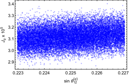
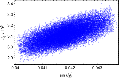
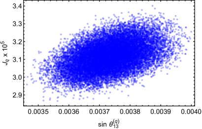
Figure 3: Correlation between the quark mixing angles and the Jarlskog invariant.

Observable	Experimental value		Model value
	$1\sigma$ range	$3\sigma$ range
$m_{e}$ [MeV]	$0.4883266(17)$	$0.4883266(51)$	0.488341
$m_{\mu}$ [MeV]	$102.87267(21)$	$102.87267(63)$	102.873
$m_{\tau}$ [MeV]	$1747.43(12)$	$1747.43(36)$	1747.43
$\Delta m_{21}^{2}$ $[10^{-5}$eV${}^{2}]$	$7.49_{-0.19}^{+0.19}$	6.92–8.05	7.49004
$\Delta m_{31}^{2}$ $[10^{-3}$eV${}^{2}]$	$2.513_{-0.019}^{+0.021}$	2.451–2.578	2.513
$\sin^{2}\theta^{(\ell)}_{12}/10^{-1}$	$3.08_{-0.11}^{+0.12}$	2.75–3.45	3.08
$\sin^{2}\theta^{(\ell)}_{23}/10^{-1}$	$4.70_{-0.13}^{+0.17}$	4.35–5.85	4.69999
$\sin^{2}\theta^{(\ell)}_{13}/10^{-2}$	$2.215^{+0.056}_{-0.058}$	2.030–2.388	2.215
$\delta^{(\ell)}_{\text{CP}}$ $[^{\circ}]$	$212_{-41}^{+26}$	124–364	211.995

Table 5: Experimental values of the SM charged lepton masses [47] and neutrino mass squared differences, leptonic mixing parameters, and CP-violating phase for the scenario of normal order neutrino mass [48] along with the model values obtained for the best fit solution corresponding to $\chi^{2}=1.46\times 10^{-9}$.

For the lepton sector, the summation in the $\chi^{2}$ function defined in Eq. (60) includes the charged lepton masses, the experimentally measured neutrino mass-squared differences, the lepton mixing angles, and the leptonic Dirac CP-violating phase. The neutrino masses are fitted under the assumption that the symmetry breaking scales are $v_{23}\sim\mathcal{O}(10)$ TeV, $v_{12}\sim\mathcal{O}(10^{3})$ TeV, and $M_{3}\sim\mathcal{O}(10^{11})$ TeV. As presented in Table 5, the model successfully reproduces the experimental data in the neutrino sector under the normal mass ordering scenario. By solving the eigenvalue problem for the charged lepton and active neutrino mass matrices, we identify a benchmark solution that yields the correct charged lepton masses, neutrino mass-squared differences, leptonic mixing angles, and the Dirac CP phase, all of which are consistent with experimental observations. This solution leads to the following forms for the mass matrices of the SM charged leptons and light active neutrinos:

$$M_{e} = \left(\begin{array}[]{ccc}-50.4475-69.6146i&55.1413-3.22028i&256.03+20.9526i\\ 25.2226+4.60226i&-11.4663+11.4492i&-374.481+673.853i\\ 0&0&-84.572+1544.43i\\ \end{array}\right)\mathrm{MeV},$$ (68)

$$M_{\nu} = \left(\begin{array}[]{ccc}-19.0017+3.14894i&-1.61237+2.90527i&1.48751+18.0746i\\ -1.61237+2.90527i&0.219646+0.529448i&2.60182+1.73744i\\ 1.48751+18.0746i&2.60182+1.73744i&38.9502+0.i\\ \end{array}\right)\mathrm{meV}.$$ (72)

The correlation among several observables in the lepton sector is illustrated in Fig. 4. It is evident that $\sin^{2}\theta_{23}^{(\ell)}$ exhibits an inverse correlation with both $\sin^{2}\theta_{13}^{(\ell)}$ and $\sin^{2}\theta_{12}^{(\ell)}$ — that is, as $\sin^{2}\theta_{23}^{(\ell)}$ increases, both $\sin^{2}\theta_{13}^{(\ell)}$ and $\sin^{2}\theta_{12}^{(\ell)}$ tend to decrease, and vice versa. Moreover, a positive correlation is observed between $\sin^{2}\theta_{23}^{(\ell)}$ and the leptonic Dirac CP-violating phase $\delta^{(\ell)}_{\text{CP}}$, implying that larger values of $\sin^{2}\theta_{23}^{(\ell)}$ correspond to an increase in $\delta^{(\ell)}_{\text{CP}}$.

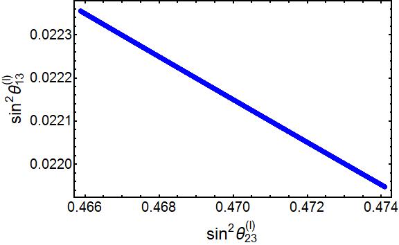
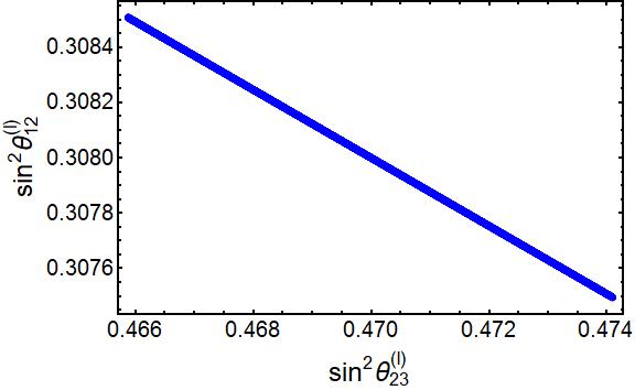
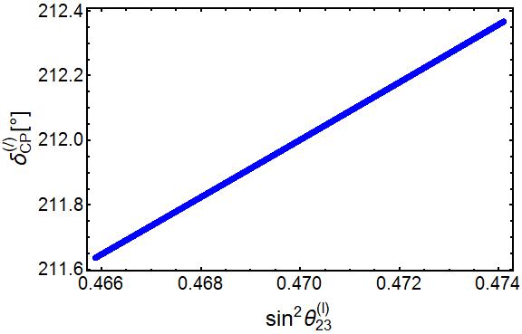
Figure 4: Correlation among some lepton sector observables.

V Electroweak precision test

V.1 $\rho$ parameter

The model under consideration predicts a tree-level mixing between the SM $Z$ boson and the new neutral gauge bosons. This mixing leads to a reduction in the physical mass of the $\mathcal{Z}$ boson relative to the SM expectation, whereas the mass of the SM $W$ boson remains unaffected. As a result, the $\rho$ parameter receives a tree-level correction, which is given by

$$\Delta\rho=\frac{m^{2}_{W}}{c_{W}^{2}m_{\mathcal{Z}}^{2}}-1\simeq\frac{9v^{2}}{10v_{23}^{2}}\left(1-\frac{g_{Y}^{2}}{g_{3}^{2}}\right)^{2}.$$ (73)

Using the global fit value, $\rho=1.00031\pm 0.00019$ [4], we derive a low bound on the new physics scale $v_{23}$, shown as the red curve in Fig. 5. In this analysis, we have taken $v=246$ GeV, $s_{W}^{2}=0.231$, $g=0.652$, and imposed $\Delta\rho=0.0005$. The shaded region corresponds to the excluded parameter space. The constraint is most stringent for $g_{3}\gtrsim 0.8$. For reference, the dashed blue line represents a natural gauge unification scenario in which the three gauge couplings are of similar magnitude, i.e., $g_{1}=g_{2}=g_{3}=\sqrt{3}g_{Y}$. In this case, we obtain the lower bounds $v_{23}\gtrsim 6.88$ TeV and $m_{Z_{23}}\gtrsim 2.78$ TeV.

V.2 $\varepsilon_{1,2}$ mixing parameters

Due to the mixing between the SM $Z$ boson and the new neutral gauge bosons $Z_{1,2}$, the well-measured vector and axial-vector couplings of the SM $Z$ boson to fermions are modified by terms proportional to the mixing parameters $\varepsilon_{1,2}$, namely,

$$g_{V,A}^{\mathcal{Z}}(f)=g_{V,A}^{Z}(f)+\mathcal{O}(\varepsilon_{1,2}),$$ (74)

as explicitly shown in Table 6 in Appendix B. According to the electroweak precision data [4], the new physics effects remain consistent with observations if $|\varepsilon_{1,2}|\lesssim 10^{-3}$ [49, 50]. Hence, we take the bound $|\varepsilon_{1}|=10^{-3}$ into account and then obtain the allowed parameter space as determined by the brown curve in Fig. 5. In the gauge unification scenario $g_{1}=g_{2}=g_{3}=\sqrt{3}g_{Y}$, this translates to the bounds $v_{23}\gtrsim 5.95$ TeV and $m_{Z_{23}}\gtrsim 2.39$ TeV.

V.3 Total $\mathcal{Z}$ decay width

The precision measurement of the total decay width of the $\mathcal{Z}$ boson allows us to place constraints on the free parameters of the model. The relevant interaction between $\mathcal{Z}$ and the SM fermions is described by the Lagrangian:

$$\mathcal{L}\supset-\frac{g}{2c_{W}}\left\{\bar{\nu}_{iL}\gamma^{\mu}\tilde{G}_{L}^{\mathcal{Z}}(\nu_{iL})(1+\delta^{\nu_{iL}})\nu_{iL}+\bar{f}\gamma^{\mu}[\tilde{G}_{V}^{\mathcal{Z}}(f)(1+\delta_{V}^{f})-\tilde{G}_{A}^{\mathcal{Z}}(f)(1+\delta_{A}^{f})\gamma_{5}]f\right\}\mathcal{Z}_{\mu},$$ (75)

where $f$ runs over all the SM charged fermions, and

$$\tilde{G}_{L}^{\mathcal{Z}}(\nu_{iL}) = \frac{1}{2}\sum_{k=1}^{3}(V^{*}_{\nu L})_{ki}(V_{\nu L})_{ki},$$ (76)

$$\tilde{G}_{V,A}^{\mathcal{Z}}(e_{i}) = \frac{1}{2}\sum_{k=1}^{3}\left[-c_{2W}(V^{*}_{eL})_{ki}(V_{eL})_{ki}\pm(1-c_{2W})(V^{*}_{eR})_{ki}(V_{eR})_{ki}\right],$$ (77)

$$\tilde{G}_{V,A}^{\mathcal{Z}}(u_{i}) = \frac{1}{6}\sum_{k=1}^{3}\left[(1+2c_{2W})(V^{*}_{uL})_{ki}(V_{uL})_{ki}\pm 2(c_{2W}-1)(V^{*}_{uR})_{ki}(V_{uR})_{ki}\right],$$ (78)

$$\tilde{G}_{V,A}^{\mathcal{Z}}(d_{i}) = \frac{1}{6}\sum_{k=1}^{3}\left[-(2+c_{2W})(V^{*}_{dL})_{ki}(V_{dL})_{ki}\pm(1-c_{2W})(V^{*}_{dR})_{ki}(V_{dR})_{ki}\right],$$ (79)

and $\delta^{\nu_{iL}}=\tilde{g}^{\mathcal{Z}}_{L}(\nu_{iL})/\tilde{G}_{L}^{\mathcal{Z}}(\nu_{iL})-1$, $\delta_{V,A}^{f}=\tilde{g}^{\mathcal{Z}}_{V,A}(f)/G_{V,A}^{\mathcal{Z}}(f)-1$, in which the couplings in mass eigenstates $\tilde{g}^{\mathcal{Z}}_{L}(\nu_{iL})$ and $\tilde{g}^{\mathcal{Z}}_{V,A}(f)$ can be extracted from the couplings collected in Table 6,

$$\tilde{g}^{\mathcal{Z}}_{L}(\nu_{iL}) = \frac{1}{2}\sum_{k=1}^{3}(V^{*}_{\nu L})_{ki}\left(g^{\mathcal{Z}}_{V}(\nu_{kL})+g^{\mathcal{Z}}_{A}(\nu_{kL})\right)(V_{\nu L})_{ki},$$ (80)

$$\tilde{g}^{\mathcal{Z}}_{V,A}(e_{i}) = \frac{1}{2}\sum_{k=1}^{3}\left[(V^{*}_{eL})_{ki}\left(g^{\mathcal{Z}}_{V}(e_{k})+g^{\mathcal{Z}}_{A}(e_{k})\right)(V_{eL})_{ki}\pm(V^{*}_{eR})_{ki}\left(g^{\mathcal{Z}}_{V}(e_{k})-g^{\mathcal{Z}}_{A}(e_{k})\right)(V_{eR})_{ki}\right],$$ (81)

$$\tilde{g}^{\mathcal{Z}}_{V,A}(u_{i}) = \tilde{g}^{\mathcal{Z}}_{V,A}(e_{i})|_{e_{k}\to u_{k},V_{eL,R}\to V_{uL,R}},$$ (82)

$$\tilde{g}^{\mathcal{Z}}_{V,A}(d_{i}) = \tilde{g}^{\mathcal{Z}}_{V,A}(e_{i})|_{e_{k}\to d_{k},V_{eL,R}\to V_{dL,R}}.$$ (83)

Hence, the total $\mathcal{Z}$ decay width predicted by our model is separated to $\Gamma_{\mathcal{Z}}=\Gamma^{\text{SM}}_{\mathcal{Z}}+\Delta\Gamma_{\mathcal{Z}}$, in which $\Gamma^{\text{SM}}_{\mathcal{Z}}$ is the SM value and the shift $\Delta\Gamma_{\mathcal{Z}}$ is given by

$$\Delta\Gamma_{\mathcal{Z}} \simeq \frac{m^{\text{SM}}_{\mathcal{Z}}}{6\pi}\frac{g^{2}}{4c^{2}_{W}}\left\{\sum_{f}N^{f}_{C}\left[\left|\tilde{G}_{V}^{\mathcal{Z}}(f)\right|^{2}\text{Re}[\delta_{V}^{f}]+\left|\tilde{G}_{A}^{\mathcal{Z}}(f)\right|^{2}\text{Re}[\delta_{A}^{f}]\right]+2\sum_{i}\left|\tilde{G}_{L}^{\mathcal{Z}}(\nu_{iL})\right|^{2}\text{Re}[\delta^{\nu_{iL}}]\right\}$$ (84)

$$+\frac{\Delta m_{\mathcal{Z}}}{12\pi}\frac{g^{2}}{4c^{2}_{W}}\left\{\sum_{f}N_{C}^{f}\left[\left|\tilde{G}_{V}^{\mathcal{Z}}(f)\right|^{2}+\left|\tilde{G}_{A}^{\mathcal{Z}}(f)\right|^{2}\right]+2\sum_{i}\left|\tilde{G}_{L}^{\mathcal{Z}}(\nu_{iL})\right|^{2}\right\},$$

where $m^{\text{SM}}_{\mathcal{Z}}$ is the SM value of the $\mathcal{Z}$-boson mass, $N_{C}^{f}$ is the color number of the fermion $f$, and the mass shift $\Delta m_{\mathcal{Z}}\simeq gvt_{W}g_{3}\varepsilon_{1}/4g_{12}$. Using the total $\mathcal{Z}$ decay width measured by the experiment $\Gamma^{\text{exp}}_{\mathcal{Z}}=2.4952\pm 0.0023$ GeV and predicted by the SM $\Gamma^{\text{SM}}_{\mathcal{Z}}=2.4942\pm 0.0008$ GeV [4], we require $|\Delta\Gamma_{\mathcal{Z}}|<0.0041$ GeV and then obtain a bound for viable parameter space regions as determined by pink curve in Fig. 5. This bound is generally lower than that given by the two previous cases.

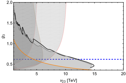
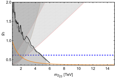
Figure 5: Red, brown, pink, orange, gray, and black curves denote the exclusion bounds derived from the $\rho$ parameter [4], $\varepsilon_{1,2}$ mixing parameters [49, 50], total $\mathcal{Z}$ decay width [4], LEPII [51], ATLAS [52] and CMS [53], respectively. The shaded regions indicate the excluded parameter space. The dashed blue line corresponds to the gauge unification condition $g_{1}=g_{2}=g_{3}=\sqrt{3}g_{Y}$.

VI Collider bounds

VI.1 LEPII

LEPII probes possess $e^{+}e^{-}\to f\bar{f}$ for $f=e,\mu,\tau$, which can be mediated by new neutral gauge bosons such as $Z_{23}$ and $Z_{12}$ [49]. Since the center-of-mass energy of the LEPII, $\sqrt{s}=209$ GeV, is much smaller than the masses of these new gauge bosons, $m_{Z_{23}}$ and $m_{Z_{12}}$, such processes can be described by effective four-fermion contact interactions, namely

$$\mathcal{L}_{\text{eff}}=\frac{g^{2}}{c^{2}_{W}}\sum_{I}\sum_{\mathcal{A,B}=L,R}\frac{1}{m^{2}_{I}}\tilde{g}_{\mathcal{A}}^{I}(e)\tilde{g}_{\mathcal{B}}^{I}(f)(\bar{e}_{\mathcal{A}}\gamma_{\mu}e_{\mathcal{A}})(\bar{f}_{\mathcal{B}}\gamma^{\mu}f_{\mathcal{B}}),$$ (85)

where $I=Z_{23},Z_{12}$, and $\tilde{g}^{I}_{L,R}(f)$ are chiral gauge couplings of boson $I$ with fermion $f$, which can be extracted from Table 7 in Appendix B as

$$\tilde{g}^{I}_{L}(f) = \frac{1}{2}\sum_{k=1}^{3}(V^{*}_{eL})_{kf}\left(g^{I}_{V}(e_{k})+g^{I}_{A}(e_{k})\right)(V_{eL})_{kf},$$ (86)

$$\tilde{g}^{I}_{R}(f) = \frac{1}{2}\sum_{k=1}^{3}(V^{*}_{eR})_{kf}\left(g^{I}_{V}(e_{k})-g^{I}_{A}(e_{k})\right)(V_{eR})_{kf}.$$ (87)

The LEPII experiment reported the lower limit of scale of these contact interaction types as $\Lambda^{\pm}_{ff}$, in which $\Lambda^{+}_{ff}$ for $\text{Re}[\tilde{g}_{\mathcal{A}}^{I}(e)(\tilde{g}_{\mathcal{B}}^{I}(f))^{*}]>0$ and $\Lambda^{-}_{ff}$ for $\text{Re}[\tilde{g}_{\mathcal{A}}^{I}(e)(\tilde{g}_{\mathcal{B}}^{I}(f))^{*}]<0$ [51]. Let us study a particular process $e^{+}e^{-}\to\mu^{+}\mu^{-}$, the mass of the $I$ boson is bounded by

$$m_{I}>\frac{g}{c_{W}}\sqrt{\frac{\left|\tilde{g}^{I}_{\mathcal{A}}(e)\tilde{g}^{I}_{\mathcal{B}}(\mu)\right|}{4\pi}}\Lambda^{\pm}_{\mu\mu}.$$ (88)

It is checked that the strongest constraint on $m_{Z_{23}}$, and thus $v_{23}$, comes from the $VV$ model with $\Lambda_{\mu\mu}^{+}=18.9$ TeV, which is displayed by orange curve in Fig. 5. In the region $g_{3}\gtrsim 0.4$, this bound is much lower than that from the LHC discussed below. However, for $g_{Y}\lesssim g_{3}\lesssim 0.4$, the LEPII constraint is significant, implying $m_{Z_{23}}\gtrsim 6$ TeV.

VI.2 LHC

At the LHC, the $Z_{23}$ boson can be directly produced in proton-proton colliders by quark-antiquark annihilation through the process $\bar{q}q\to Z_{23}$. Once created, the heavy $Z_{23}$ boson subsequently decays into a pair of quarks (dijet channel) or a pair of charged leptons (dilepton channel). In the context of our model, the most promising and sensitive probe is provided by the dilepton decay modes, $Z_{23}\to ll$ with $l=e,\mu$. The production cross section for these processes can be calculated using the narrow width approximation, under the assumption that $\Gamma_{Z_{23}}\ll m_{Z_{23}}$, which yields:

$$\sigma(pp\to Z_{23}\to l\bar{l})\simeq\frac{1}{3}\sum_{q}\frac{dL_{q\bar{q}}}{dm^{2}_{Z_{23}}}\hat{\sigma}(q\bar{q}\to Z_{23})\mathrm{Br}(Z_{23}\to l\bar{l}),$$ (89)

where the luminosity $dL_{q\bar{q}}/dm^{2}_{Z_{23}}$ can be extracted from Ref. [54]. The partonic peak cross-section $\hat{\sigma}(q\bar{q}\to Z_{23})$ and the branching decay ratio $\mathrm{Br}(Z_{23}\to l\bar{l})=\Gamma(Z_{23}\to l\bar{l})/\sum_{f}\Gamma(Z_{23}\to f\bar{f})$ are given by

$$\hat{\sigma}(q\bar{q}\to Z_{23})=\frac{\pi g^{2}}{12c^{2}_{W}}\left(|\tilde{g}^{Z_{23}}_{V}(q)|^{2}+|\tilde{g}^{Z_{23}}_{A}(q)|^{2}\right),$$ (90)

$$\Gamma(Z_{23}\to f\bar{f})=\frac{g^{2}m_{Z_{23}}}{48\pi c^{2}_{W}}N_{C}^{f}\left(|\tilde{g}^{Z_{23}}_{V}(f)|^{2}+|\tilde{g}^{Z_{23}}_{A}(f)|^{2}\right),$$ (91)

in which $f$ is all the SM fermions, and the relevant couplings are given by Eqs. (80–83). Above, we have assumed that the decay channels of $Z_{23}$ into right-handed neutrinos and new scalars negligibly contribute to the total decay width of $Z_{23}$.

The bound of parameter space induced by the process $pp\to Z^{\prime}\to l\bar{l}$ with the latest ATLAS [52] (CMS [53]) constraint taking width per resonance mass to be 3% (0.6%) is shown in Fig. 5 by a black (gray) curve. This bound is strongest for $0.4\lesssim g_{3}\lesssim 0.8$ and implies that in gauge unification scenario $g_{1}=g_{2}=g_{3}=\sqrt{3}g_{Y}$ then $v_{23}\gtrsim 12$ TeV and $m_{Z_{23}}\gtrsim 4.9$ TeV.

VII Flavor constraints

Due to the non-universal charge assignments of fermion generations under the gauge group $U(1)_{Y_{1}}\otimes U(1)_{Y_{2}}\otimes U(1)_{Y_{3}}$, the model naturally contains tree-level flavor-changing neutral currents (FCNCs). These are mediated by the heavy gauge bosons $Z_{12}$ and $Z_{23}$, as well as the SM $Z$ boson, and contribute to $\Delta F=2$ processes, such as meson mass differences $\Delta m_{P}$ ($P=K,B_{s},B_{d},D$). It is important to note that the parameters $y^{d}_{i}$, which account for the observed fermion mass hierarchies and mixing, are taken to be real. Consequently, the model does not introduce new sources of CP violation in neutral meson mixing or rare decay processes. Additionally, the FCNC interactions also affect several $b\to sll$ observables and lepton flavor-violating decays. In this work, we provide a more detailed analysis of the FCNC phenomenology than in previous studies, such as Refs. [41, 42].

The effective Hamiltonian relevant for FCNCs $\Delta F=2$ processes can be expressed as

$$\mathcal{H}^{\Delta F=2}_{\text{eff}} = \frac{G_{F}^{2}m_{W}^{2}}{16\pi^{2}}\left\{(V^{*}_{tq}V_{tb})^{2}[(C^{q}_{\text{SM}}+C^{q}_{LL})(\bar{b}_{L}\gamma_{\mu}q_{L})^{2}+C^{q}_{RR}(\bar{b}_{R}\gamma_{\mu}q_{R})^{2}+C^{q}_{LR}(\bar{b}_{L}\gamma_{\mu}q_{L})(\bar{b}_{R}\gamma^{\mu}q_{R})]\right.$$ (92)

$$+\left.(V^{*}_{ts}V_{td})^{2}[(C^{K}_{\text{SM}}+C^{K}_{LL})(\bar{s}_{L}\gamma_{\mu}d_{L})^{2}+C^{K}_{RR}(\bar{s}_{R}\gamma_{\mu}d_{R})^{2}+C^{K}_{LR}(\bar{s}_{L}\gamma_{\mu}d_{L})(\bar{s}_{R}\gamma^{\mu}d_{R})]\right\},$$

where the first and second part describes for $B_{q}$ ($q=d,s$) and $K$ mixings, respectively. Additionally, $C^{q,K}_{\text{SM}}$ are SM Wilson coefficients for $B_{q},K$ meson mixings, which read [55]

$$C^{q}_{\text{SM}} = 4S_{0}(x_{t})\eta_{B},$$ (93)

$$C^{K}_{\text{SM}} = 4\eta_{1}(\lambda_{c}/\lambda_{t})^{2}S_{0}(x_{c})+4\eta_{2}S_{0}(x_{t})+8\eta_{3}(\lambda_{c}/\lambda_{t})S_{0}(x_{c},x_{t}),$$ (94)

where $x_{t(c)}=m_{t(c)}^{2}/m_{W}^{2}$, $\lambda_{t(c)}=V^{*}_{t(c)s}V_{t(c)d}$, while $S_{0}$ is the Inami-Lim function [56], and the factors $\eta_{B,1,2,3}$ are next-to-leading order (NLO) QCD corrections [55]. The new physics (NP) Wilson coefficients $C^{q,K}_{LL,RR,LR}$ are defined at the matching scale $\mu=m_{Z_{12}}$ or $m_{Z_{23}}$, i.e.,

$$C^{q}_{LL} = \frac{16\pi^{2}}{G_{F}^{2}m_{W}^{2}(V^{*}_{tq}V_{tb})^{2}}\left[\frac{([\Gamma^{Z_{12}}_{L}]_{3q})^{2}}{m_{Z_{12}}^{2}}+\frac{([\Gamma^{Z_{23}}_{L}]_{3q})^{2}}{m_{Z_{23}}^{2}}+\frac{([\Gamma^{Z}_{L}]_{3q})^{2}}{m_{Z}^{2}}\right],$$ (95)

$$C^{q}_{RR} = \frac{16\pi^{2}}{G_{F}^{2}m_{W}^{2}(V^{*}_{tq}V_{tb})^{2}}\left[\frac{([\Gamma^{Z_{12}}_{R}]_{3q})^{2}}{m_{Z_{12}}^{2}}+\frac{([\Gamma^{Z_{23}}_{R}]_{3q})^{2}}{m_{Z_{23}}^{2}}+\frac{([\Gamma^{Z}_{R}]_{3q})^{2}}{m_{Z}^{2}}\right],$$ (96)

$$C^{q}_{LR} = \frac{16\pi^{2}}{G_{F}^{2}m_{W}^{2}(V^{*}_{tq}V_{tb})^{2}}\left[\frac{[\Gamma^{Z_{12}}_{L}]_{3q}[\Gamma^{Z_{12}}_{R}]_{3q}}{m_{Z_{12}}^{2}}+\frac{[\Gamma^{Z_{23}}_{L}]_{3q}[\Gamma^{Z_{23}}_{R}]_{3q}}{m_{Z_{23}}^{2}}+\frac{[\Gamma^{Z}_{L}]_{3q}[\Gamma^{Z}_{R}]_{3q}}{m_{Z}^{2}}\right],$$ (97)

$$C^{K}_{LL} = \frac{16\pi^{2}}{G_{F}^{2}m_{W}^{2}(V^{*}_{ts}V_{td})^{2}}\left[\frac{([\Gamma^{Z_{12}}_{L}]_{21})^{2}}{m_{Z_{12}}^{2}}+\frac{([\Gamma^{Z_{23}}_{L}]_{21})^{2}}{m_{Z_{23}}^{2}}+\frac{([\Gamma^{Z}_{L}]_{21})^{2}}{m_{Z}^{2}}\right],$$ (98)

$$C^{K}_{RR} = \frac{16\pi^{2}}{G_{F}^{2}m_{W}^{2}(V^{*}_{ts}V_{td})^{2}}\left[\frac{([\Gamma^{Z_{12}}_{R}]_{21})^{2}}{m_{Z_{12}}^{2}}+\frac{([\Gamma^{Z_{23}}_{R}]_{21})^{2}}{m_{Z_{23}}^{2}}+\frac{([\Gamma^{Z}_{R}]_{21})^{2}}{m_{Z}^{2}}\right],$$ (99)

$$C^{K}_{LR} = \frac{16\pi^{2}}{G_{F}^{2}m_{W}^{2}(V^{*}_{ts}V_{td})^{2}}\left[\frac{[\Gamma^{Z_{12}}_{L}]_{21}[\Gamma^{Z_{12}}_{R}]_{21}}{m_{Z_{12}}^{2}}+\frac{[\Gamma^{Z_{23}}_{L}]_{21}[\Gamma^{Z_{23}}_{R}]_{21}}{m_{Z_{23}}^{2}}+\frac{[\Gamma^{Z}_{L}]_{21}[\Gamma^{Z}_{R}]_{21}}{m_{Z}^{2}}\right],$$ (100)

where the flavor-violating couplings $[\Gamma^{Z_{12},Z_{23},Z}_{L(R)}]_{ij}$ induced by gauge bosons $Z_{12},Z_{23},Z$ are generally have the below forms

$$[\Gamma^{Z_{12}}_{L(R)}]_{ij} = -g_{1}Y^{L(R)}_{1}s_{12}(V^{*}_{q_{L(R)}})_{1i}(V_{q_{L(R)}})_{1j}+g_{2}Y^{L(R)}_{2}c_{12}(V^{*}_{q_{L(R)}})_{2i}(V_{q_{L(R)}})_{2j},$$ (101)

$$[\Gamma^{Z_{23}}_{L(R)}]_{ij} = -g_{12}Y_{1}^{L(R)}s_{23}(V^{*}_{q_{L(R)}})_{1i}(V_{q_{L(R)}})_{1j}+g_{12}Y_{2}^{L(R)}s_{23}(V^{*}_{q_{L(R)}})_{2i}(V_{q_{L(R)}})_{2j}$$ (102)

$$+g_{3}Y_{3}^{L(R)}c_{23}(V^{*}_{q_{L(R)}})_{3i}(V_{q_{L(R)}})_{3j},$$

$$[\Gamma^{Z}_{L}]_{ij} = (T_{3L}g_{L}c_{W}-Y_{1}^{L}s_{W}g_{Y})(V^{*}_{q_{L}})_{1i}(V_{q_{L}})_{1j}+(T_{3L}g_{L}c_{W}-Y_{2}^{L}s_{W}g_{Y})(V^{*}_{q_{L}})_{2i}(V_{q_{L}})_{2j}$$ (103)

$$+(T_{3L}g_{L}c_{W}-Y_{3}^{L}s_{W}g_{Y})(V^{*}_{q_{L}})_{3i}(V_{q_{L}})_{3j},$$

$$[\Gamma^{Z}_{R}]_{ij} = -Y_{1}^{R}s_{W}g_{Y}(V^{*}_{q_{R}})_{1i}(V_{q_{R}})_{1j}-Y_{2}^{R}s_{W}g_{Y}(V^{*}_{q_{R}})_{2i}(V_{q_{R}})_{2j}-Y_{3}^{R}s_{W}g_{Y}(V^{*}_{q_{R}})_{3i}(V_{q_{R}})_{3j},$$ (104)

in which $Y^{L,R}_{i}$ are hypercharges for $q_{iL,R}$, i.e $Y^{L}=\left\{1/6,1/6\right\}$ for $u_{iL},d_{iL}$, $Y^{R}=\left\{2/3,-1/3\right\}$ for $u_{iR},d_{iR}$. The unitary matrices $V_{q_{L,R}}$ connect the weak and mass eigenstates, which can be numerically obtained by benchmark points that successfully reproduce the fermion spectrum, as shown in Table 4. It should be noted that with $Y^{1}_{L}=Y^{2}_{L}=Y^{3}_{L}$, the flavor-violating couplings of SM $Z$ boson $[\Gamma^{Z}_{L(R)}]_{ij}$ vanish, due to the unitary condition of $V_{qL(R)}$, i.e $[\Gamma^{Z}_{L(R)}]_{ij}\sim\sum_{k=1}^{3}[V^{*}_{qL(R)}]_{ki}[V_{qL(R)}]_{kj}=0$ with $i\neq j$. In addition, the terms depend on $1/m^{2}_{Z_{12}}$ in the above WCs can be skipped due to a very high scale $m_{Z_{12}}\sim v_{12}\sim\mathcal{O}(10^{3})$ TeV. This leads the WCs in $\Delta F=2$ processes depend mostly on $m_{Z_{23}}$ and couplings $g_{12},g_{3}$.

With the effective Hamiltonian for $\Delta F=2$ processes in Eq. (92), we can determine the ratios between SM+NP contribution with SM ones in meson mass difference $\Delta m_{P}$ as follows

$$\epsilon_{K} = \frac{\Delta m_{K}^{\text{SM}}+\Delta m_{K}^{\text{NP}}}{\Delta m_{K}^{\text{SM}}}=\frac{\text{Re}[M_{12}^{K,\text{NP}}+M_{12}^{K,\text{SM}}]}{\text{Re}[M_{12}^{K,\text{SM}}]}$$ (105)

$$= \frac{1}{\text{Re}[C^{K}_{\text{SM}}]}\text{Re}\left\{(C^{K}_{LL}+C^{K}_{RR})\eta_{K}^{6/23}-C^{K}_{LR}\left[\frac{3}{2}+\left(\frac{m_{K}}{m_{d}+m_{s}}\right)^{2}\right]\eta_{K}^{3/23}\frac{B_{K}^{(5)}}{B_{K}^{(1)}}\right.$$

$$+\left.C^{K}_{LR}\left[\frac{1}{6}+\left(\frac{m_{K}}{m_{d}+m_{s}}\right)^{2}\right]\left(\eta_{K}^{3/23}-\eta_{K}^{-24/23}\right)\frac{B^{(4)}_{K}}{B_{K}^{(1)}}\right\},$$

$$\epsilon_{B_{q}} = \frac{\Delta m_{B_{q}}^{\text{SM+NP}}}{\Delta m_{B_{q}}^{\text{SM}}}=\left|1+\frac{M_{12}^{q,\text{NP}}}{M_{12}^{q,\text{SM}}}\right|$$ (106)

$$= \left|1+\frac{C^{q}_{LL}+C^{q}_{RR}}{C^{q}_{\text{SM}}}\eta_{B_{q}}^{6/23}-\frac{C^{q}_{LR}}{C^{q}_{\text{SM}}}\left[\frac{3}{2}+\left(\frac{m_{B_{q}}}{m_{q}+m_{b}}\right)^{2}\right]\eta_{B_{q}}^{3/23}\frac{B_{B_{q}}^{(5)}}{B_{B_{q}}^{(1)}}\right.$$

$$+\left.\frac{C^{q}_{LR}}{C^{q}_{\text{SM}}}\left[\frac{1}{6}+\left(\frac{m_{B_{q}}}{m_{q}+m_{b}}\right)^{2}\right]\left(\eta_{B_{q}}^{3/23}-\eta_{B_{q}}^{-24/23}\right)\frac{B_{B_{q}}^{(4)}}{B_{B_{q}}^{(1)}}\right|,$$

where the hadronic matrix elements are expressed in terms of non-perturbative bag parameters $B_{P}^{(i)}$ as follows

$$\langle P|(\bar{q}_{iL}\gamma_{\mu}q_{jL})^{2}|\bar{P}\rangle = \langle P|(\bar{q}_{iR}\gamma_{\mu}q_{jR})^{2}|\bar{P}\rangle=\frac{2}{3}m_{P}^{2}f_{P}^{2}B_{P}^{(1)}(\mu),$$ (107)

$$\langle P|(\bar{q}_{iL}q_{jR})(\bar{q}_{iR}q_{jL})|\bar{P}\rangle = \frac{1}{2}\left[\frac{1}{6}+\frac{m_{P}^{2}}{(m_{q_{i}}+m_{q_{j}})^{2}}\right]m_{P}^{2}f_{P}^{2}B_{P}^{(4)}(\mu),$$ (108)

$$\langle P|(\bar{q}_{iL}\gamma_{\mu}q_{jL})(\bar{q}_{iR}\gamma_{\mu}q_{jR})|\bar{P}\rangle = -2\langle P|(\bar{q}^{\alpha}_{iL}q^{\beta}_{jR})(\bar{q}^{\beta}_{iR}q_{jL}^{\alpha})|\bar{P}\rangle$$ (109)

$$= -\frac{1}{3}\left[\frac{3}{2}+\frac{m_{P}^{2}}{(m_{q_{i}}+m_{q_{j}})^{2}}\right]m_{P}^{2}f_{P}^{2}B_{P}^{(5)}(\mu),$$

with $\alpha,\beta$ to be color indices. The third line appears due to the Fierz transformation of the LR operator. In addition, the coefficients $\eta_{P}\equiv\alpha_{s}(\mu_{\text{NP}})/\alpha_{s}(\mu_{P})$ present the QCD corrections at leading order (LO) approximation by using renormalization group evolution (RGE) from NP scale $\mu_{\text{NP}}=m_{Z_{23}}$ to the hadronic scale $\mu_{P}\sim 3$ GeV for $K$ meson and $\mu_{P}=4.16$ GeV for $B_{s,d}$ mesons [57]. It is important to note that these running effects lead to operator mixing in non-color singlet LR operators. Thus, there exist both bag parameters $B_{4}$ and $B_{5}$ in Eqs. (105) and (106). In order to estimate the impact of NP to $\Delta m_{P}$, we adapt the following 2$\sigma$ constraints given in [29],

$$\frac{\Delta m_{B_{s}}^{\text{SM+NP}}}{\Delta m_{B_{s}}^{\text{SM}}}=\frac{\Delta m_{B_{s}}^{\text{exp}}}{\Delta m_{B_{s}}^{\text{SM}}}\in[0.8597,1.0332],$$ (110)

$$\frac{\Delta m_{B_{d}}^{\text{SM+NP}}}{\Delta m_{B_{d}}^{\text{SM}}}=\frac{\Delta m_{B_{d}}^{\text{exp}}}{\Delta m_{B_{d}}^{\text{SM}}}\in[0.8336,1.0335],$$ (111)

for $B_{s}$ and $B_{d}$ mesons. For the $K$ meson, the uncertainty of the SM prediction $\Delta m_{K}^{\text{SM}}$ is considerable compared to the $B_{s,d}$ meson systems, due to the difficulty in theoretical approaches for long-distance effects. Therefore, the constraint for $\Delta m_{K}$ is not strong as $\Delta m_{B_{s,d}}$, and we ignore this constraint in the considering work.

The flavor-violating couplings induced by $Z_{12},Z_{23},Z$ also contribute to several $\Delta S=1$ processes such as $b\to sl^{+}l^{-}$ decays, which can be described by the following effective Hamiltonian,

$$\mathcal{H}^{\Delta S=1}_{\text{eff}} = -\frac{4G_{F}(V^{*}_{ts}V_{tb})}{\sqrt{2}}\sum_{I=9,10}(C_{I}^{\text{SM}}+C_{I}^{\text{NP}})\mathcal{O}_{I}+C_{I}^{{}^{\prime}\text{NP}}\mathcal{O}^{{}^{\prime}}_{I}$$ (112)

with $C_{I}^{\text{SM}}$ are SM WCs which are calculated at NNLO, while $C_{I}^{(^{\prime})\text{NP}}$ are NP contributions. The operators and their corresponding Wilson coefficients (at the scale $\mu=m_{Z_{23}}$) are

$$[\mathcal{O}^{(^{\prime})}_{9}]_{ij} = \frac{e^{2}}{16\pi^{2}}(\bar{s}_{L(R)}\gamma_{\mu}b_{L(R)})(\bar{e}_{i}\gamma^{\mu}e_{j}),$$ (113)

$$[C^{(^{\prime})\text{NP}}_{9}]_{ij} \simeq \frac{16\pi^{2}}{e^{2}}\frac{g\sqrt{2}}{8G_{F}(V^{*}_{ts}V_{tb})c_{W}}\frac{[\Gamma^{Z_{23}}_{L}]_{23}[\tilde{g}^{Z_{23}}_{V}]_{ij}}{m_{Z_{23}}^{2}},$$ (114)

$$[\mathcal{O}^{(^{\prime})}_{10}]_{ij} = \frac{e^{2}}{16\pi^{2}}(\bar{s}_{L(R)}\gamma_{\mu}b_{L(R)})(\bar{e}_{i}\gamma^{\mu}\gamma_{5}e_{j}),$$ (115)

$$[C^{(^{\prime})\text{NP}}_{10}]_{ij} \simeq -\frac{16\pi^{2}}{e^{2}}\frac{g\sqrt{2}}{8G_{F}(V^{*}_{ts}V_{tb})c_{W}}\frac{[\Gamma^{Z_{23}}_{L}]_{23}[\tilde{g}^{Z_{23}}_{A}]_{ij}}{m_{Z_{23}}^{2}},$$ (116)

where

$$[\tilde{g}^{Z_{23}}_{V,A}]_{ij}=\frac{1}{2}\sum_{k=1}^{3}\left[(V^{*}_{eL})_{ki}\left(g^{Z_{23}}_{V}(e_{k})+g^{Z_{23}}_{A}(e_{k})\right)(V_{eL})_{kj}\pm(V^{*}_{eR})_{ki}\left(g^{Z_{23}}_{V}(e_{k})-g^{Z_{23}}_{A}(e_{k})\right)(V_{eR})_{kj}\right]$$ (117)

are vector and axial-vector couplings induced by new gauge boson $Z_{23}$ in mass eigenstates, while $g^{Z_{23}}_{V,A}(e_{k})$ are vector and axial-vector couplings in flavor states and given explicitly in Tables 6 and 7.

We want to emphasize that there are no significant NP contributions to Wilson coefficients of dipole operators $C^{(^{\prime})}_{7}$. This can be explained because $C^{(^{\prime})}_{7}$ are induced by one-loop involving FCNCs couplings of $Z_{12},Z_{23}$, which are very suppressed by factor $m_{W}^{2}/m^{2}_{Z_{23}}\ll 1$ for $m_{Z_{23}}\sim\mathcal{O}(10)$ TeV. Therefore, the model provides NP contributions for four Wilson coefficients $C^{(^{\prime})}_{9}$ and $C^{(^{\prime})}_{10}$. The SM+NP contribution normalized to SM one in the branching ratio of $B_{s}\to\mu^{+}\mu^{-}$ is given in

$$\epsilon_{B_{s}\to\mu^{+}\mu^{-}} = \frac{\text{BR}(B_{s}\to\mu^{+}\mu^{-})_{\text{SM+NP}}}{\text{BR}(B_{s}\to\mu^{+}\mu^{-})_{\text{SM}}}=\frac{\text{BR}(B_{s}\to\mu^{+}\mu^{-})_{\text{exp}}}{\text{BR}(B_{s}\to\mu^{+}\mu^{-})_{\text{SM}}}$$ (118)

$$= \frac{1}{1-y_{s}}\frac{|C_{10}^{\text{SM}}+C^{\text{NP}}_{10}-C^{{}^{\prime}\text{NP}}_{10}|^{2}}{|C^{SM}_{10}|^{2}}.$$

In order to estimate the NP impact, we consider the predicted $\epsilon_{B_{s}\to\mu^{+}\mu^{-}}$ with corresponding $2\sigma$ range

$$\frac{\text{BR}(B_{s}\to\mu^{+}\mu^{-})_{\text{exp}}}{\text{BR}(B_{s}\to\mu^{+}\mu^{-})_{\text{SM}}}\in[0.7574,1.0778],$$ (119)

where $\text{BR}(B_{s}\to\mu^{+}\mu^{-})_{\text{exp}}=3.34(27)\times 10^{-9}$ [58] and SM prediction including power-enhanced QED correction is $\text{BR}(B_{s}\to\mu^{+}\mu^{-})_{\text{SM}}=3.64(12)\times 10^{-9}$ [4].

For scenarios of lepton flavor violating decaying $B_{s}\to l_{i}^{+}l_{j}^{-}$ ($i\neq j$), we adapt the result in [59] as follows

$$\text{BR}(B_{s}\to l_{i}^{+}l_{j}^{-}) = \frac{\alpha^{2}G_{F}^{2}|V^{*}_{ts}V_{tb}|^{2}m_{B_{s}}f_{B_{s}}^{2}\tau_{B_{s}}\text{Max}[m_{i}^{2},m^{2}_{j}]}{64\pi^{3}}\left(1-\frac{\text{Max}[m_{i}^{2},m^{2}_{j}]}{m_{B_{s}}^{2}}\right)^{2}$$ (120)

$$\times\left(|[C^{\text{NP}}_{9}]_{ij}-[C^{{}^{\prime}\text{NP}}_{9}]_{ij}|^{2}+|[C_{10}^{\text{NP}}]_{ij}-[C^{{}^{\prime}\text{NP}}_{10}]_{ij}|^{2}\right).$$

Among above processes with different product lepton flavors $(e\mu,e\tau,\mu\tau)$, we concentrate on the ones with decaying lepton flavors $e^{+}\mu^{-}$ since they have strongest constraint, namely BR$(B_{s}\to e^{\pm}\mu^{\mp})_{\text{exp}}<5.4\times 10^{-9}$ [4].

The flavor-violating interactions of $Z_{12},Z_{23}$ also appear in the lepton sector, which can make the leptonic three-body decays at tree-level, such as $\tau\to 3\mu,3e$ and $\mu\to 3e$. The branching ratio of these processes is shown by

$$\text{BR}(e_{i}\to 3e_{j}) = \frac{m_{i}^{5}\eta^{2}_{\text{RGE}}}{1536\pi^{3}\Gamma_{e_{i}}m^{4}_{Z_{23}}}\left[2(|[\tilde{g}^{Z_{23}}_{L}]_{ji}[\tilde{g}^{Z_{23}}_{L}]_{jj}|^{2}+|[\tilde{g}^{Z_{23}}_{R}]_{ji}[\tilde{g}^{Z_{23}}_{R}]_{jj}|^{2})\right.$$ (121)

$$\left.+|[\tilde{g}^{Z_{23}}_{L}]_{ji}[\tilde{g}^{Z_{23}}_{R}]_{jj}|^{2}+|[\tilde{g}^{Z_{23}}_{R}]_{ji}[\tilde{g}^{Z_{23}}_{L}]_{jj}|^{2}\right],$$

for $i\neq j$, $i=\mu,\tau$ and $j=e,\mu$. The factor $\eta_{\text{RGE}}$ presents for RGE running from high scale $\mu\sim m_{Z_{23}}\sim\mathcal{O}(10)$ TeV to low scale $\mu\sim 1$ GeV, which numerically is $\eta_{\text{RGE}}\sim 0.9$ [42]. In addition, the couplings $[\tilde{g}^{Z_{23}}_{L(R)}]_{ij}$ are given in Eq. (117). Besides three-body leptonic decays, there exist loop contributions involving $Z_{23}$ and SM charged lepton $e_{k}$ to radiative decays $e_{i}\to e_{j}\gamma$. Their branching ratios are given in the limit $m_{e_{i}}\gg m_{e_{j}}$ and $m_{e_{k}}^{2}/m^{2}_{Z_{23}}\ll 1$ as follow

$$\text{BR}(e_{i}\to e_{j}\gamma) = \frac{m_{j}^{3}}{4\pi\Gamma_{e_{j}}}\left(|[C^{Z_{23}}_{L}]_{ij}|^{2}+|[C^{Z_{23}}_{R}]_{ij}|^{2}\right),$$ (122)

with coefficients $[C^{Z_{23}}_{L(R)}]_{ij}$ read

$$[C^{Z_{23}}_{L(R)}]_{ij} \simeq \frac{e\eta_{\text{RGE}}}{48\pi^{2}m^{2}_{Z_{23}}}\sum_{k=e,\mu,\tau}\left(m_{e_{j}}[\tilde{g}^{Z_{23}}_{R(L)}]_{ik}[\tilde{g}^{Z_{23}}_{R(L)}]_{kj}-3m_{k}[\tilde{g}^{Z_{23}}_{R(L)}]_{ik}[\tilde{g}^{Z_{23}}_{L(R)}]_{kj}\right.$$ (123)

$$\left.+m_{i}[\tilde{g}^{Z_{23}}_{L(R)}]_{ik}[\tilde{g}^{Z_{23}}_{L(R)}]_{kj}\right).$$

For numerical study, we focus on the observables having the strongest experimental constraints, BR$(\mu\to 3e)_{\text{exp}}<1.0\times 10^{-12}$ and BR$(\mu\to e\gamma)_{\text{exp}}<4.2\times 10^{-13}$ [4].

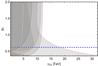
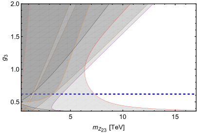
Figure 6: Black, brown, orange, pink, red, and purple curves denote the exclusion bounds derived from $\epsilon_{B_{s}}$, $\epsilon_{B_{d}}$, $\epsilon_{B_{s}\to\mu^{+}\mu^{-}}$, BR$(B_{s}\to e^{\pm}\mu^{\mp})$, BR$(\mu\to 3e)$, and BR$(\mu\to e\gamma)$, respectively. The shaded regions indicate the excluded parameter space. The dashed blue line corresponds to the gauge unification scenario $g_{1}=g_{2}=g_{3}=\sqrt{3}g_{Y}$.

In Fig. 6, we show the correlation between the coupling $g_{3}$ of gauge group $U(1)_{Y_{3}}$ and the VEV $v_{23}$ satisfying constraints of $\epsilon_{B_{s}}$ (black), $\epsilon_{B_{d}}$ (brown), $\epsilon_{B_{s}\to\mu^{+}\mu^{-}}$ (orange), BR$(B_{s}\to e^{\pm}\mu^{\mp})$ (pink), BR$(\mu\to 3e)$ (red), and BR$(\mu\to e\gamma)$ (purple). The parameter space, as indicated by the shaded regions, is excluded. We see that the process $\mu\to 3e$ ($\mu\to e\gamma$) gives the strongest constraint if $g_{3}\lesssim 1$ ($g_{3}\gtrsim 1$). At $g_{3}\simeq 1$ then $v_{23}$ and $m_{Z_{23}}$ are minimal, i.e., $v_{23}\simeq 11.6$ TeV and $m_{Z_{23}}\simeq 6.3$ TeV. For the gauge unification case $g_{1}=g_{2}=g_{3}=\sqrt{3}g_{Y}$, we have $v_{23}\gtrsim 18.6$ TeV and $m_{Z_{23}}\gtrsim 7.3$ TeV. These lower bounds are larger than the bounds given in sections V and VI.

VIII Majorana Dark matter

Since the dark scalars $R_{1,2}$, $I_{1,2}$ and $\eta^{\pm}$ are extremely heavy, with masses at the scale $v_{12}\sim\mathcal{O}(10^{3})$ TeV, while the dark fermions $N_{1,2R}$ reside at a lower scale $\Lambda\sim\mathcal{O}(1)$ TeV, our model predicts a distinctive DM candidate: the right-handed Majorana neutrino, stabilized by the conservation of dark parity. Without loss of generality, we assume that $N_{1R}$ is the lightest among the dark-sector fields responsible for DM. In this section, the mixing angles $\theta_{R,I}$ are neglected due to their strong suppression. Additionally, for simplicity, we ignore mixings between $H_{2}$ and $H_{3,4}$, as well as between $\nu_{1R}$ and $\nu_{2R}$, effectively taking $\mathsf{H}\simeq H_{2}$, $N_{1R}\simeq\nu_{1R}$, and $N_{2R}\simeq\nu_{2R}$.

VIII.1 Dark matter relic abundance

As discussed in Section IV.2, the radiative contribution to active neutrino masses is significant and consistent with experimental observations, even for Yukawa coupling of order $\kappa\sim\mathcal{O}(1)$. This implies that the DM candidate $N_{1R}$ is appreciably coupled to the SM particles in the thermal bath of the early Universe. Consequently, the freeze-out mechanism is operative and determines both the DM relic abundance and the DM nature as a weakly interacting massive particle. The dominant processes for DM pair annihilation involve final states consisting of the SM particle pairs, and—when kinematically allowed—pairs of the new bosons $\mathsf{H}$ and $\mathsf{Z}$, as shown in Fig. 7. It is important to note that, due to the Majorana nature of $N_{1R}$, each $t$-channel annihilation diagram has a corresponding $u$-channel diagram, although only the former are explicitly shown in the figure. Additionally, the vector-like fermions and all fields with mass at the $v_{12,23}$ scales are significantly heavier than $N_{1R}$, and thus are kinematically inaccessible as final states in DM annihilation processes.

Figure 7: Annihilations govern the DM relic density, where $\ell=e,\mu,\tau$ and $\nu=\nu_{e},\nu_{\mu},\nu_{\tau}$.

The thermal average annihilation cross section times relative velocity for the $N_{1R}$ DM can be decomposed into four parts, namely

$$\langle\sigma v_{\text{rel}}\rangle_{N_{1R}} = \langle\sigma v_{\text{rel}}\rangle_{N_{1R}N_{1R}\to\text{SMSM}}+\langle\sigma v_{\text{rel}}\rangle_{N_{1R}N_{1R}\to\mathsf{HH}}$$ (124)

$$+\langle\sigma v_{\text{rel}}\rangle_{N_{1R}N_{1R}\to\mathsf{ZH}}+\langle\sigma v_{\text{rel}}\rangle_{N_{1R}N_{1R}\to\mathsf{ZZ}},$$

where the first part is related to the DM annihilation to the SM particles, while the remaining parts are the DM annihilation to the new bosons. In the non-relativistic approximation, it is straightforward to determine

$$\langle\sigma v_{\text{rel}}\rangle_{N_{1R}} \simeq \frac{\lambda_{3}^{2}M_{1}^{2}}{128\pi}\left[\frac{3m_{h}^{2}}{m_{\mathsf{H}}^{2}(4M_{1}^{2}-m_{h}^{2})}-\frac{1}{4M_{1}^{2}-m_{\mathsf{H}}^{2}}\right]^{2}\left(1-\frac{m_{h}^{2}}{M_{1}^{2}}\right)^{\frac{1}{2}}$$ (125)

$$+\frac{3\epsilon_{2}^{2}M_{1}^{6}}{8\pi v^{2}\Lambda^{2}}\left(\frac{1}{4M_{1}^{2}-m_{\mathsf{H}}^{2}}-\frac{1}{4M_{1}^{2}-m_{h}^{2}}\right)^{2}$$

$$+\frac{\epsilon_{2}^{2}m_{t}^{2}M_{1}^{4}}{8\pi v^{2}\Lambda^{2}}\left(\frac{1}{4M_{1}^{2}-m_{\mathsf{H}}^{2}}-\frac{1}{4M_{1}^{2}-m_{h}^{2}}\right)^{2}\left(1-\frac{m_{t}^{2}}{M_{1}^{2}}\right)^{\frac{3}{2}}$$

$$+\frac{\kappa^{4}M_{1}^{2}}{32\pi}\left[\frac{1}{(M_{1}^{2}+m_{\eta^{0}}^{2})^{2}}+\frac{1}{(M_{1}^{2}+m_{\eta^{\pm}}^{2})^{2}}\right]$$

$$+\frac{M_{1}^{2}}{128\pi\Lambda^{4}}\left[\frac{9m_{\mathsf{H}}^{4}}{(4M_{1}^{2}-m_{\mathsf{H}}^{2})^{2}}+\frac{32M_{1}^{4}(M_{1}^{2}-m_{\mathsf{H}}^{2})^{2}}{(2M_{1}^{2}-m_{\mathsf{H}}^{2})^{4}x_{F}}-\frac{12M_{1}^{2}m_{\mathsf{H}}^{2}(M_{1}^{2}-m_{\mathsf{H}}^{2})}{(4M_{1}^{2}-m_{\mathsf{H}}^{2})(2M_{1}^{2}-m_{\mathsf{H}}^{2})^{2}x_{F}}\right]$$

$$\times\left(1-\frac{m_{\mathsf{H}}^{2}}{M_{1}^{2}}\right)^{\frac{1}{2}}\Theta(M_{1}-m_{\mathsf{H}})$$

$$+\frac{g^{4}_{\mathsf{D}}}{64\pi M_{1}^{4}m_{\mathsf{Z}}^{4}}[m^{4}_{\mathsf{H}}-2m^{2}_{\mathsf{H}}(4M_{1}^{2}+m^{2}_{\mathsf{Z}})+(4M_{1}^{2}-m^{2}_{\mathsf{Z}})^{2}]^{\frac{3}{2}}\Theta\left(M_{1}-\frac{m_{\mathsf{Z}}+m_{\mathsf{H}}}{2}\right)$$

$$+\frac{g_{\mathsf{D}}^{4}}{16\pi M_{1}^{2}}\left[1+\frac{2M_{1}^{4}(8M_{1}^{4}+m^{4}_{\mathsf{H}})}{m^{4}_{\mathsf{Z}}(4M_{1}^{2}-m^{2}_{\mathsf{H}})^{2}x_{F}}\right]\left(1-\frac{m_{\mathsf{Z}}^{2}}{M_{1}^{2}}\right)^{\frac{1}{2}}\Theta(M_{1}-m_{\mathsf{Z}}),$$

for which only the dominant channels are presented. Here, $\Theta(\cdots)$ is the Heaviside step function, $x_{F}=M_{1}/T_{F}\simeq 25$ is given at freeze-out temperature, and $m_{\eta^{0}}\simeq m_{R_{1},I_{1}}$. As shown in the left panel of Fig. 8, the new Higgs mass resonance $M_{1}=m_{\mathsf{H}}/2$ and, when kinematically accessible, the annihilation channel $N_{1R}N_{1R}\to\mathsf{ZH}$ are crucial to set the correct DM relic density $\Omega_{\text{DM}}h^{2}\simeq 0.12$ [3], where we have taken $m_{\eta^{0}}=m_{\eta^{\pm}}=100\text{ TeV}$, $\kappa=1$, $g_{\mathsf{D}}=\sqrt{3}g_{Y}\simeq 0.619$, $\lambda_{3}=0.1$, $\lambda_{2}=0.3$, $\Lambda=2.46$ TeV, and $\epsilon_{2}=0.01$, in addition $v=246$ GeV, $m_{t}=173$ GeV, and $m_{h}=125$ GeV. In the right panel, we present the contours corresponding to the observed DM relic density in the ($M_{1},\Lambda$) plane for various values of $\lambda_{2}$, while keeping all other parameters fixed as in the previous analysis. For each value of $\lambda_{2}$, three distinct curves emerge. Among them, two nearly parallel curves arise due to the mass resonance associated with the new Higgs boson. In contrast, the remaining curve is predominantly governed by the $\mathsf{Z}\mathsf{H}$ annihilation channel. From these results, we conclude that the dark fermion $N_{1R}$, with a mass in the TeV range, can successfully account for the observed DM relic abundance.

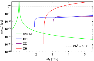
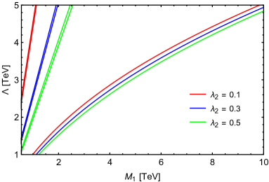
Figure 8: Left panel: DM annihilation cross sections into various final states as functions of the DM mass. Right panel: Contours of the observed DM relic density in the plane of DM mass versus the new physics scale, shown for different values of the coupling $\lambda_{2}$.

VIII.2 Dark matter scattering off nuclei

We now turn our attention to the direct detection prospects of the dark fermion $N_{1R}$. Although $N_{1R}$ does not couple directly to the SM quarks, its scattering with nucleons can occur via Higgs mediation. In particular, due to the mixing between the SM Higgs doublet $H$ and the new scalar singlet $\Phi$, there exist tree-level elastic scattering processes mediated by the Higgs bosons $h$ and $\mathsf{H}$ through $t$-channel exchange, as illustrated in the first diagram of Fig. 9. In addition to the tree-level contribution, one-loop processes also contribute to DM–nucleon scattering. These arise from effective couplings of $N_{1R}$ to the $h$ and $\mathsf{H}$ scalar bosons and to the SM $Z$ boson, as depicted in the remaining diagrams of the figure.

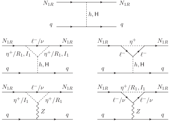
Figure 9: Diagrams for DM-nucleon scattering, where $\ell=e,\mu,\tau$ and $\nu=\nu_{e},\nu_{\mu},\nu_{\tau}$.

Let us consider the first scenario, where the mixing parameter $\epsilon_{2}$ is quite large, i.e., $\epsilon_{2}\simeq 0.01$, as mentioned above. In such a case, the dominant contribution to the scattering process $N_{1R}$-nucleons results from the first diagram of Fig. 9. The effective Lagrangian describing this scattering process is given by

$$\mathcal{L}_{\mathrm{eff}}=C_{q}(\bar{N}_{R}^{c}N_{R})(\bar{q}q),$$ (126)

in which the effective coupling is

$$C_{q}=-\frac{\epsilon_{2}m_{q}M_{1}}{\Lambda v}\left(\frac{1}{m^{2}_{h}}-\frac{1}{m^{2}_{\mathsf{H}}}\right)\simeq-\frac{\epsilon_{2}m_{q}M_{1}}{\Lambda vm^{2}_{h}},$$ (127)

where $m_{q}$ denotes the $q$ quark mass. Additionally, the contribution of $\mathsf{H}$ is negligible in comparison to that of $h$, and is thus omitted. Then, the spin-independent (SI) elastic scattering cross-section of $N_{1R}$ per nucleon $N$ can be written as

$$\sigma^{\mathrm{SI}}_{N_{1R}}=\frac{4}{\pi}\left(\frac{M_{1}m_{N}}{M_{1}+m_{N}}\right)^{2}\left[\frac{\text{Z}f_{p}+(\text{A}-\text{Z})f_{n}}{\text{A}}\right]^{2},$$ (128)

where A and Z respectively are the mass and atomic number of the target nucleus, $m_{N}$ is the average nucleon mass. In addition, the interaction strengths of proton $f_{p}$ and neutron $f_{n}$ with the dark fermion $N_{1R}$ is given by

$$f_{p,n}=m_{p,n}\left(\sum_{q=u,d,s}f_{Tq}^{p,n}\frac{C_{q}}{m_{q}}+\frac{2}{27}f_{TG}^{p,n}\sum_{q=c,b,t}\frac{C_{q}}{m_{q}}\right)$$ (129)

with $f_{TG}^{p,n}=1-\sum_{q=u,d,s}f_{Tq}^{p,n}$. Here, $m_{p,n}$ are the proton and neutron masses, respectively. Additionally, the parameters $f^{p,n}_{Tq}$ are evaluated as $f^{p}_{Tu}=0.020\pm 0.004$, $f^{p}_{Td}=0.026\pm 0.005$, $f^{p}_{Ts}=0.118\pm 0.062$, $f^{n}_{Tu}=0.014\pm 0.003$, $f^{n}_{Td}=0.036\pm 0.008$, and $f^{n}_{Ts}=0.118\pm 0.062$ [60].

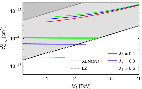
Figure 10: SI scattering cross section of the DM candidate $N_{1R}$ with nucleons as a function of the DM mass. Solid curves represent theoretical predictions. The dashed gray (black) curve shows current experimental bounds from XENON1T [61] (LZ [62]). Shaded regions are excluded by these experiments.

Taking $\text{A}=131$, $\text{Z}=54$, $m_{p}\simeq m_{n}\simeq m_{N}=1$ GeV, $m_{u}=2.16$ MeV, $m_{d}=4.7$ MeV, $m_{s}=93.5$ MeV, $m_{c}=1.273$ GeV, $m_{b}=4.183$ GeV, together with the previously adopted parameter values that yield the correct DM relic density, we present in Fig. 10 the contours in the ($M_{1},\sigma^{\text{SI}}_{N_{1R}}$) plane. For comparison, we also include the most stringent current bounds on the SI scattering cross section from the XENON1T and LZ experiments [61, 62]. As shown, all curves satisfying the relic density constraint are consistent with the XENON1T limit. However, a large portion of these curves is excluded by the LZ limit, depending on the value of $\lambda_{2}$. For instance, the LZ bound requires $2.1\text{ TeV}\lesssim M_{1}\lesssim 2.8$ TeV when $\lambda_{2}=0.3$. Furthermore, the projected sensitivity of upcoming direct detection experiments such as XENONnT [63] and LZ [64] is expected to probe deeper into the parameter space, typically favoring $\epsilon_{2}<0.01$.

Alternatively, we consider the scenario in which the mixing parameter $\epsilon_{2}$ is extremely small, i.e., $\epsilon_{2}\lesssim 10^{-5}$, while the quartic couplings $\lambda_{32,39}$ and the Yukawa coupling $\kappa$ are sizable, specifically $\lambda_{32,39}\simeq 2\pi$ and $\kappa\simeq 2\sqrt{\pi}$. In this case, the previous results for the correct DM relic density remain essentially unchanged. However, the dominant contribution to the $N_{1R}$-nucleons scattering process now arises from the one-loop diagrams shown in the second row of Fig. 9. The corresponding effective coupling is given by

$$C_{q}\simeq-\frac{\kappa^{2}m_{q}}{16\pi^{2}m_{h}^{2}M_{1}}\left[\lambda_{32}\mathcal{G}_{1}\left(\frac{M_{1}^{2}}{m_{\eta^{\pm}}^{2}}\right)+\frac{\lambda_{32}+\lambda_{39}}{2}\mathcal{G}_{2}\left(\frac{M_{1}^{2}}{m_{\eta^{0}}^{2}}\right)\right],$$ (130)

where the loop function is defined as $\mathcal{G}_{1}(x)=[x+(1-x)\ln(1-x)]/x$. Taking the parameter values as above, we estimate the SI scattering cross-section of $N_{1R}$ per nucleon $N$ as

$$\sigma^{\mathrm{SI}}_{N_{1R}}\lesssim\left(\frac{M_{1}}{\text{TeV}}\right)^{2}\times 6.3\times 10^{-52}\text{ cm}^{2}.$$ (131)

This result is in agreement with the current bounds provided by the XENON1T and LZ experiments [61, 62], even the projected bounds from upcoming direct detection experiments such as XENONnT [63] and LZ [64].

Last but not least, we consider the possibility that the $N_{1R}$-nucleons scattering process is predominantly mediated by the exchange of the SM $Z$-boson, as described by the one-loop diagrams in the third row of Fig. 9. This results in an effective axial-vector interaction of the form $A_{q}\bar{N}_{1R}\gamma^{\mu}\gamma^{5}N_{1R}\bar{q}\gamma_{\mu}\gamma^{5}q$, in which

$$A_{q}=\frac{\kappa^{2}g_{A}^{q}}{32\pi^{2}m_{Z}^{2}}\left[(g_{V}^{\ell}+g_{A}^{\ell})\mathcal{G}_{2}\left(\frac{M_{1}^{2}}{m^{2}_{\eta^{\pm}}}\right)+(g_{V}^{\nu}+g_{A}^{\nu})\mathcal{G}_{2}\left(\frac{M_{1}^{2}}{m^{2}_{\eta^{0}}}\right)\right]$$ (132)

with the loop function $\mathcal{G}_{2}(x)=2[x+(1-x)\ln(1-x)]/x^{2}-1$ and the couplings $g_{A}^{q}=\frac{1}{2}\left(-\frac{1}{2}\right)$ for $q=u,c,t~(d,s,b)$, $g_{V}^{\ell}=-\frac{g}{2c_{W}}\left(\frac{1}{2}-2s_{W}^{2}\right)$, $g_{A}^{\ell}=-\frac{g}{4c_{W}}$, $g_{V}^{\nu}=g_{A}^{\nu}=\frac{g}{4c_{W}}$. Hence, the spin-dependent (SD) scattering cross section of $N_{1R}$ in the case of the proton target is given by

$$\sigma^{\mathrm{SD}}_{N_{1R}}=\frac{16}{\pi}\left(\frac{M_{1}m_{p}}{M_{1}+m_{p}}\right)^{2}J_{p}(J_{p}+1)A_{p}^{2}$$ (133)

with $A_{p}=\sum_{q=u,d,s}\lambda_{q}^{p}A_{q}$. Here, the fractional quark-spin coefficients are $\lambda^{p}_{u}=0.85$, $\lambda^{p}_{d}=-0.42$, and $\lambda^{p}_{s}=-0.08$, while the angular momentum of the target nucleus in this case is $J_{p}=1/2$ [65]. Taking $s_{W}^{2}=0.231$, $g=0.652$, $m_{Z}=91.188$ GeV, and the previous parameter values, we obtain

$$\sigma^{\mathrm{SD}}_{N_{1R}}\lesssim\left(\frac{M_{1}}{\text{TeV}}\right)^{4}\times 5.08\times 10^{-49}\text{ cm}^{2},$$ (134)

given that $\kappa\lesssim 2\sqrt{\pi}$. The predicted result by our model lies well below the sensitivity of present experiments [62, 66, 67] and projected experiments [63, 64].

IX Conclusion

The hierarchical structure of fermion masses suggests that the SM fermion generations may not be universal at high energy scales. This motivates the hypothesis that SM fermions could carry family-dependent hypercharges, analogous to individual lepton numbers. In contrast, right-handed neutrinos, being singlets under the SM gauge group, may instead be charged under a distinct dark gauge symmetry, decoupled from the SM fermion sector.

To explore this possibility, we have constructed a minimal and renormalizable extension of the SM—namely, the fully flipped inert doublet model—supplemented by scalar singlets, vector-like charged fermions, and right-handed Majorana neutrinos. These new fields are essential for generating the observed mass hierarchies of SM charged fermions through higher-dimensional operators, while the small active neutrino masses are realized via a hybrid mechanism combining tree-level Type-I seesaw and one-loop scotogenic contributions.

A residual dark parity, originating from the gauge structure, guarantees the stability of the lightest parity-odd particle, thus providing a viable DM candidate in the form of a dark Majorana neutrino. This symmetry also plays a central role in the radiative generation of neutrino masses. Furthermore, the decomposition of the SM hypercharge into three generation-specific hypercharges offers a natural explanation for the existence of exactly three fermion families.

In summary, the proposed framework presents a unified, minimal, and renormalizable solution to three fundamental puzzles in the SM: the origin of neutrino masses, the nature of DM, and the fermion flavor structure. The model is shown to be consistent with current experimental constraints from electroweak precision measurements, collider searches, flavor-changing processes, and DM observations, thereby offering a promising direction for physics beyond the SM.

Appendix A General hypercharge decomposition

Because the anomalies associated with the hypercharge are canceled within each fermion generation, as in the SM, there is no fundamental reason that each generation hypercharge must correspond uniquely to a single fermion generation. In other words, multiple fermion generations may, in principle, share the same generation hypercharge. Consequently, the number of fermion generations remains theoretically unconstrained. For completeness, we consider a generalized decomposition of the SM hypercharge as $Y=\sum_{n=1}^{\mathcal{N}}Y_{n}$, with $Y_{n}=YC_{n}$, and investigate a particular form of the coefficient $C_{n}$ that can provide a theoretical insight into this generational puzzle, i.e.,

$$C_{n}=\frac{2^{(2+n-n^{2})/2}}{(-1)^{n}}\frac{(4-n)_{\mathcal{N}-3}}{(n)_{1-2n+\mathcal{N}}}\frac{(1-a)_{N}}{(a-n)(N-n)!},$$ (135)

where $a$ is a generation index, $a=1,2,\cdots,N$, for $N$ and $\mathcal{N}$ to be arbitrary integer. Additionally, we have used the Pochhammer function $(x)_{y}=x(x+1)\ldots(x+y-1)$. It is worthwhile that the above form of $C_{n}$ induces $C_{n}=0$ if $n\geq 4$, reducing to

$$Y=Y_{1}+Y_{2}+Y_{3}.$$ (136)

Additionally, $C_{1}=C_{2}=C_{3}=0$ if $a\geq 4$ gives a suitable argument for the existence of only three fermion generations as observed. Furthermore, for $a\leq 3$, we obtain

$$C_{1} = \frac{1}{2}(a-2)(a-3),$$

$$C_{2} = -(a-1)(a-3),$$

$$C_{3} = \frac{1}{2}(a-1)(a-2),$$ (137)

implying $C_{1}=1$ and $C_{2}=C_{3}=0$ if $a=1$, $C_{2}=1$ and $C_{1}=C_{3}=0$ if $a=2$, $C_{3}=1$ and $C_{1}=C_{2}=0$ if $a=3$. These mean that each of the three fermion generations is charged under only a separate hypercharge gauge symmetry.

Appendix B Vector and axial-vector couplings

The interactions between the gauge bosons and the SM fermions originate from the fermion kinetic term, $\sum_{F}\bar{F}i\gamma^{\mu}D_{\mu}F$, where $F$ runs over all SM fermion multiplets. It is straightforward to verify that the gluon, photon, and $W$-boson interactions with the SM fermions remain identical to those in the SM. In addition, the interaction of the neutral gauge bosons $Z_{I}=\mathcal{Z},Z_{23},Z_{12}$ with the SM fermions takes the form

$$\mathcal{L}\supset-\frac{g}{2c_{W}}\bar{f}\gamma^{\mu}[g_{V}^{Z_{I}}(f)-g_{A}^{Z_{I}}(f)\gamma_{5}]fZ_{I\mu},$$ (138)

where $f$ denotes the SM fermions in the interaction basis. The vector ($g_{V}$) and axial-vector ($g_{A}$) couplings of the SM fermions to the $\mathcal{Z}$ boson are summarized in Table 6. As expected, these couplings reduce to those of the SM $Z$ boson in the limit $\varepsilon_{1,2}\to 0$. Table 7 lists the corresponding couplings for the gauge bosons $Z_{23}$ and $Z_{12}$ in the simplifying limit $\varepsilon_{1,2},\zeta\to 0$. Notably, $Z_{12}$ does not couple to the third fermion generation and exhibits flavor non-universal couplings for the first and second generations. In contrast, $Z_{23}$ features flavor-universal couplings for the first two generations, while the couplings to the third generation are distinct.

$f$	$g_{V}^{\mathcal{Z}}(f)$	$g_{A}^{\mathcal{Z}}(f)$
$\nu_{1}$	$\frac{1}{2}-\frac{g_{1}c_{W}(c_{12}s_{23}\varepsilon_{1}+s_{12}\varepsilon_{2})}{2g}$	$\frac{1}{2}-\frac{g_{1}c_{W}(c_{12}s_{23}\varepsilon_{1}+s_{12}\varepsilon_{2})}{2g}$
$\nu_{2}$	$\frac{1}{2}-\frac{g_{2}c_{W}(s_{12}s_{23}\varepsilon_{1}-c_{12}\varepsilon_{2})}{2g}$	$\frac{1}{2}-\frac{g_{2}c_{W}(s_{12}s_{23}\varepsilon_{1}-c_{12}\varepsilon_{2})}{2g}$
$\nu_{3}$	$\frac{1}{2}+\frac{g_{3}c_{W}c_{23}\varepsilon_{1}}{2g}$	$\frac{1}{2}+\frac{g_{3}c_{W}c_{23}\varepsilon_{1}}{2g}$
$e_{1}$	$\frac{1-2c_{2W}}{2}-\frac{3g_{1}c_{W}(c_{12}s_{23}\varepsilon_{1}+s_{12}\varepsilon_{2})}{2g}$	$-\frac{1}{2}+\frac{g_{1}c_{W}(c_{12}s_{23}\varepsilon_{1}+s_{12}\varepsilon_{2})}{2g}$
$e_{2}$	$\frac{1-2c_{2W}}{2}-\frac{3g_{2}c_{W}(s_{12}s_{23}\varepsilon_{1}-c_{12}\varepsilon_{2})}{2g}$	$-\frac{1}{2}+\frac{g_{2}c_{W}(s_{12}s_{23}\varepsilon_{1}-c_{12}\varepsilon_{2})}{2g}$
$e_{3}$	$\frac{1-2c_{2W}}{2}+\frac{3g_{3}c_{W}c_{23}\varepsilon_{1}}{2g}$	$-\frac{1}{2}-\frac{g_{3}c_{W}c_{23}\varepsilon_{1}}{2g}$
$u_{1}$	$\frac{4c_{2W}-1}{6}+\frac{5g_{1}c_{W}(c_{12}s_{23}\varepsilon_{1}+s_{12}\varepsilon_{2})}{6g}$	$\frac{1}{2}-\frac{g_{1}c_{W}(c_{12}s_{23}\varepsilon_{1}+s_{12}\varepsilon_{2})}{2g}$
$u_{2}$	$\frac{4c_{2W}-1}{6}+\frac{5g_{2}c_{W}(s_{12}s_{23}\varepsilon_{1}-c_{12}\varepsilon_{2})}{6g}$	$\frac{1}{2}-\frac{g_{2}c_{W}(s_{12}s_{23}\varepsilon_{1}-c_{12}\varepsilon_{2})}{2g}$
$u_{3}$	$\frac{4c_{2W}-1}{6}-\frac{5g_{3}c_{W}c_{23}\varepsilon_{1}}{6g}$	$\frac{1}{2}+\frac{g_{3}c_{W}c_{23}\varepsilon_{1}}{2g}$
$d_{1}$	$-\frac{1+2c_{2W}}{6}-\frac{g_{1}c_{W}(c_{12}s_{23}\varepsilon_{1}+s_{12}\varepsilon_{2})}{6g}$	$-\frac{1}{2}+\frac{g_{1}c_{W}(c_{12}s_{23}\varepsilon_{1}+s_{12}\varepsilon_{2})}{2g}$
$d_{2}$	$-\frac{1+2c_{2W}}{6}-\frac{g_{2}c_{W}(s_{12}s_{23}\varepsilon_{1}-c_{12}\varepsilon_{2})}{6g}$	$-\frac{1}{2}+\frac{g_{2}c_{W}(s_{12}s_{23}\varepsilon_{1}-c_{12}\varepsilon_{2})}{2g}$
$d_{3}$	$-\frac{1+2c_{2W}}{6}+\frac{g_{3}c_{W}c_{23}\varepsilon_{1}}{6g}$	$-\frac{1}{2}-\frac{g_{3}c_{W}c_{23}\varepsilon_{1}}{2g}$

Table 6: The couplings of the $\mathcal{Z}$ gauge boson with the SM fermions.

$f$	$g_{V}^{Z_{23}}(f)$	$g_{A}^{Z_{23}}(f)$	$g_{V}^{Z_{12}}(f)$	$g_{A}^{Z_{12}}(f)$
$\nu_{1}$	$\frac{g_{12}c_{W}s_{23}}{2g}$	$\frac{g_{12}c_{W}s_{23}}{2g}$	$\frac{g_{1}c_{W}s_{12}}{2g}$	$\frac{g_{1}c_{W}s_{12}}{2g}$
$\nu_{2}$	$\frac{g_{12}c_{W}s_{23}}{2g}$	$\frac{g_{12}c_{W}s_{23}}{2g}$	$-\frac{g_{2}c_{W}c_{12}}{2g}$	$-\frac{g_{2}c_{W}c_{12}}{2g}$
$\nu_{3}$	$-\frac{g_{3}c_{W}c_{23}}{2g}$	$-\frac{g_{3}c_{W}c_{23}}{2g}$	$0$	$0$
$e_{1}$	$\frac{3g_{12}c_{W}s_{23}}{2g}$	$-\frac{g_{12}c_{W}s_{23}}{2g}$	$\frac{3g_{1}c_{W}s_{12}}{2g}$	$-\frac{g_{1}c_{W}s_{12}}{2g}$
$e_{2}$	$\frac{3g_{12}c_{W}s_{23}}{2g}$	$-\frac{g_{12}c_{W}s_{23}}{2g}$	$-\frac{3g_{2}c_{W}c_{12}}{2g}$	$\frac{g_{2}c_{W}c_{12}}{2g}$
$e_{3}$	$-\frac{3g_{3}c_{W}c_{23}}{2g}$	$\frac{g_{3}c_{W}c_{23}}{2g}$	$0$	$0$
$u_{1}$	$-\frac{5g_{12}c_{W}s_{23}}{6g}$	$\frac{g_{12}c_{W}s_{23}}{2g}$	$-\frac{5g_{1}c_{W}s_{12}}{6g}$	$\frac{g_{1}c_{W}s_{12}}{2g}$
$u_{2}$	$-\frac{5g_{12}c_{W}s_{23}}{6g}$	$\frac{g_{12}c_{W}s_{23}}{2g}$	$\frac{5g_{2}c_{W}c_{12}}{6g}$	$-\frac{g_{2}c_{W}c_{12}}{2g}$
$u_{3}$	$\frac{5g_{3}c_{W}c_{23}}{6g}$	$-\frac{g_{3}c_{W}c_{23}}{2g}$	$0$	$0$
$d_{1}$	$\frac{g_{12}c_{W}s_{23}}{6g}$	$-\frac{g_{12}c_{W}s_{23}}{2g}$	$\frac{g_{1}c_{W}s_{12}}{6g}$	$-\frac{g_{1}c_{W}s_{12}}{2g}$
$d_{2}$	$\frac{g_{12}c_{W}s_{23}}{6g}$	$-\frac{g_{12}c_{W}s_{23}}{2g}$	$-\frac{g_{2}c_{W}c_{12}}{6g}$	$\frac{g_{2}c_{W}c_{12}}{2g}$
$d_{3}$	$-\frac{g_{3}c_{W}c_{23}}{6g}$	$\frac{g_{3}c_{W}c_{23}}{2g}$	$0$	$0$

Table 7: The couplings of the $Z_{23,12}$ gauge bosons with the SM fermions in the limit $\varepsilon_{1,2},\zeta\to 0$.

References

- [1] T. Kajita, Nobel Lecture: Discovery of atmospheric neutrino oscillations, Rev. Mod. Phys. 88 (2016) 030501.
- [2] A. B. McDonald, Nobel Lecture: The Sudbury Neutrino Observatory: Observation of flavor change for solar neutrinos, Rev. Mod. Phys. 88 (2016) 030502.
- [3] Planck collaboration, Planck 2018 results. VI. Cosmological parameters, Astron. Astrophys. 641 (2020) A6 [1807.06209].
- [4] Particle Data Group collaboration, Review of particle physics, Phys. Rev. D 110 (2024) 030001.
- [5] P. Minkowski, at a Rate of One Out of Muon Decays?, Phys. Lett. B 67 (1977) 421.
- [6] M. Gell-Mann, P. Ramond and R. Slansky, Complex Spinors and Unified Theories, Conf. Proc. C 790927 (1979) 315 [1306.4669].
- [7] T. Yanagida, Horizontal gauge symmetry and masses of neutrinos, Conf. Proc. C 7902131 (1979) 95.
- [8] S. L. Glashow, The Future of Elementary Particle Physics, NATO Sci. Ser. B 61 (1980) 687.
- [9] R. N. Mohapatra and G. Senjanovic, Neutrino Mass and Spontaneous Parity Nonconservation, Phys. Rev. Lett. 44 (1980) 912.
- [10] R. N. Mohapatra and G. Senjanovic, Neutrino Masses and Mixings in Gauge Models with Spontaneous Parity Violation, Phys. Rev. D 23 (1981) 165.
- [11] G. Lazarides, Q. Shafi and C. Wetterich, Proton Lifetime and Fermion Masses in an SO(10) Model, Nucl. Phys. B 181 (1981) 287.
- [12] J. Schechter and J. W. F. Valle, Neutrino Masses in SU(2) x U(1) Theories, Phys. Rev. D 22 (1980) 2227.
- [13] J. Schechter and J. W. F. Valle, Neutrino Decay and Spontaneous Violation of Lepton Number, Phys. Rev. D 25 (1982) 774.
- [14] D. Van Loi, P. Van Dong, N. T. Duy and N. H. Thao, Questions of flavor physics and neutrino mass from a flipped hypercharge, Phys. Rev. D 109 (2024) 115022 [2312.12836].
- [15] A. Zee, A Theory of Lepton Number Violation, Neutrino Majorana Mass, and Oscillation, Phys. Lett. B 93 (1980) 389.
- [16] A. Zee, Quantum Numbers of Majorana Neutrino Masses, Nucl. Phys. B 264 (1986) 99.
- [17] K. S. Babu, Model of ’Calculable’ Majorana Neutrino Masses, Phys. Lett. B 203 (1988) 132.
- [18] L. M. Krauss, S. Nasri and M. Trodden, A Model for neutrino masses and dark matter, Phys. Rev. D 67 (2003) 085002 [hep-ph/0210389].
- [19] E. Ma, Verifiable radiative seesaw mechanism of neutrino mass and dark matter, Phys. Rev. D 73 (2006) 077301 [hep-ph/0601225].
- [20] D. Van Loi and P. Van Dong, Flavor-dependent U(1) extension inspired by lepton, baryon and color numbers, Eur. Phys. J. C 83 (2023) 1048 [2307.13493].
- [21] P. Van Dong and D. Van Loi, Scotogenic model from an extended electroweak symmetry, Phys. Rev. D 110 (2024) 035003 [2309.12091].
- [22] J. Kubo and D. Suematsu, Neutrino masses and CDM in a non-supersymmetric model, Phys. Lett. B 643 (2006) 336 [hep-ph/0610006].
- [23] N. Rojas, R. Srivastava and J. W. F. Valle, Simplest Scoto-Seesaw Mechanism, Phys. Lett. B 789 (2019) 132 [1807.11447].
- [24] D. M. Barreiros, F. R. Joaquim, R. Srivastava and J. W. F. Valle, Minimal scoto-seesaw mechanism with spontaneous CP violation, JHEP 04 (2021) 249 [2012.05189].
- [25] S. Mandal, R. Srivastava and J. W. F. Valle, The simplest scoto-seesaw model: WIMP dark matter phenomenology and Higgs vacuum stability, Phys. Lett. B 819 (2021) 136458 [2104.13401].
- [26] J. Ganguly, J. Gluza and B. Karmakar, Common origin of 13 and dark matter within the flavor symmetric scoto-seesaw framework, JHEP 11 (2022) 074 [2209.08610].
- [27] R. Kumar, P. Mishra, M. K. Behera, R. Mohanta and R. Srivastava, Predictions from scoto-seesaw with A4 modular symmetry, Phys. Lett. B 853 (2024) 138635 [2310.02363].
- [28] P. Van Dong and D. Van Loi, Scotoseesaw model implied by dark right-handed neutrinos, 2311.09795.
- [29] D. Van Loi, N. T. Duy, C. H. Nam and P. Van Dong, Scoto-seesaw model implied by flavor-dependent Abelian gauge charge, 2409.06393.
- [30] P. Van Dong, D. Van Loi, D. T. Huong, N. T. Duy and D. Van Soa, Dark symmetry implication for right-handed neutrinos, 2407.02324.
- [31] V. Silveira and A. Zee, SCALAR PHANTOMS, Phys. Lett. B 161 (1985) 136.
- [32] L. M. Krauss and F. Wilczek, Discrete Gauge Symmetry in Continuum Theories, Phys. Rev. Lett. 62 (1989) 1221.
- [33] S. P. Martin, A Supersymmetry primer, Adv. Ser. Direct. High Energy Phys. 18 (1998) 1 [hep-ph/9709356].
- [34] P. H. Frampton, Chiral dilepton model and the flavor question, Phys. Rev. Lett. 69 (1992) 2889.
- [35] P. Van Dong, T. N. Hung and D. Van Loi, Abelian charge inspired by family number, Eur. Phys. J. C 83 (2023) 199 [2212.13155].
- [36] C. D. Froggatt and H. B. Nielsen, Hierarchy of Quark Masses, Cabibbo Angles and CP Violation, Nucl. Phys. B 147 (1979) 277.
- [37] S. Rajpoot, Some Consequences of Extending the SU(5) Gauge Symmetry to the Generation Symmetry SU(5) X SU(5) X SU(5) , Phys. Rev. D 24 (1981) 1890.
- [38] X. Li and E. Ma, Gauge Model of Generation Nonuniversality, Phys. Rev. Lett. 47 (1981) 1788.
- [39] R. Barbieri, G. R. Dvali and A. Strumia, Fermion masses and mixings in a flavor symmetric GUT, Nucl. Phys. B 435 (1995) 102 [hep-ph/9407239].
- [40] C. D. Carone and H. Murayama, Third family flavor physics in an x SU(2) -L x U(1) -Y model, Phys. Rev. D 52 (1995) 4159 [hep-ph/9504393].
- [41] M. Fernández Navarro and S. F. King, Tri-hypercharge: a separate gauged weak hypercharge for each fermion family as the origin of flavour, JHEP 08 (2023) 020 [2305.07690].
- [42] M. Fernández Navarro, S. F. King and A. Vicente, Minimal complete tri-hypercharge theories of flavour, JHEP 07 (2024) 147 [2404.12442].
- [43] M. Lindner, D. Schmidt and A. Watanabe, Dark matter and U(1)’ symmetry for the right-handed neutrinos, Phys. Rev. D 89 (2014) 013007 [1310.6582].
- [44] UTfit collaboration, New UTfit Analysis of the Unitarity Triangle in the Cabibbo-Kobayashi-Maskawa scheme, Rend. Lincei Sci. Fis. Nat. 34 (2023) 37 [2212.03894].
- [45] S. F. King, Large mixing angle MSW and atmospheric neutrinos from single right-handed neutrino dominance and U(1) family symmetry, Nucl. Phys. B 576 (2000) 85 [hep-ph/9912492].
- [46] P. Van Dong, Interpreting dark matter solution for B-L gauge symmetry, Phys. Rev. D 108 (2023) 115022 [2305.19197].
- [47] Z.-z. Xing, Flavor structures of charged fermions and massive neutrinos, Phys. Rept. 854 (2020) 1 [1909.09610].
- [48] I. Esteban, M. C. Gonzalez-Garcia, M. Maltoni, I. Martinez-Soler, J. a. P. Pinheiro and T. Schwetz, NuFit-6.0: updated global analysis of three-flavor neutrino oscillations, JHEP 12 (2024) 216 [2410.05380].
- [49] ALEPH, DELPHI, L3, OPAL, SLD, LEP Electroweak Working Group, SLD Electroweak Group, SLD Heavy Flavour Group collaboration, Precision electroweak measurements on the resonance, Phys. Rept. 427 (2006) 257 [hep-ex/0509008].
- [50] J. Erler, P. Langacker, S. Munir and E. Rojas, Improved Constraints on Z-prime Bosons from Electroweak Precision Data, JHEP 08 (2009) 017 [0906.2435].
- [51] ALEPH, DELPHI, L3, OPAL, LEP Electroweak collaboration, Electroweak Measurements in Electron-Positron Collisions at W-Boson-Pair Energies at LEP, Phys. Rept. 532 (2013) 119 [1302.3415].
- [52] ATLAS collaboration, Search for high-mass dilepton resonances using 139 fb-1 of collision data collected at 13 TeV with the ATLAS detector, Phys. Lett. B 796 (2019) 68 [1903.06248].
- [53] CMS collaboration, Search for resonant and nonresonant new phenomena in high-mass dilepton final states at = 13 TeV, JHEP 07 (2021) 208 [2103.02708].
- [54] A. D. Martin, W. J. Stirling, R. S. Thorne and G. Watt, Parton distributions for the LHC, Eur. Phys. J. C 63 (2009) 189 [0901.0002].
- [55] A. J. Buras, F. De Fazio, J. Girrbach and M. V. Carlucci, The Anatomy of Quark Flavour Observables in 331 Models in the Flavour Precision Era, JHEP 02 (2013) 023 [1211.1237].
- [56] T. Inami and C. S. Lim, Effects of Superheavy Quarks and Leptons in Low-Energy Weak Processes k(L) — mu anti-mu, K+ — pi+ Neutrino anti-neutrino and K0 — anti-K0, Prog. Theor. Phys. 65 (1981) 297.
- [57] J. A. Bagger, K. T. Matchev and R.-J. Zhang, QCD corrections to flavor changing neutral currents in the supersymmetric standard model, Phys. Lett. B 412 (1997) 77 [hep-ph/9707225].
- [58] M. Czaja and M. Misiak, Current Status of the Standard Model Prediction for the Branching Ratio, Symmetry 16 (2024) 917 [2407.03810].
- [59] A. Crivellin, L. Hofer, J. Matias, U. Nierste, S. Pokorski and J. Rosiek, Lepton-flavour violating decays in generic models, Phys. Rev. D 92 (2015) 054013 [1504.07928].
- [60] J. R. Ellis, A. Ferstl and K. A. Olive, Reevaluation of the elastic scattering of supersymmetric dark matter, Phys. Lett. B 481 (2000) 304 [hep-ph/0001005].
- [61] XENON collaboration, Dark Matter Search Results from a One Ton-Year Exposure of XENON1T, Phys. Rev. Lett. 121 (2018) 111302 [1805.12562].
- [62] LZ collaboration, Dark Matter Search Results from 4.2 Tonne-Years of Exposure of the LUX-ZEPLIN (LZ) Experiment, 2410.17036.
- [63] XENON collaboration, Projected WIMP sensitivity of the XENONnT dark matter experiment, JCAP 11 (2020) 031 [2007.08796].
- [64] LZ collaboration, Projected WIMP sensitivity of the LUX-ZEPLIN dark matter experiment, Phys. Rev. D 101 (2020) 052002 [1802.06039].
- [65] H.-Y. Cheng and C.-W. Chiang, Revisiting Scalar and Pseudoscalar Couplings with Nucleons, JHEP 07 (2012) 009 [1202.1292].
- [66] XENON collaboration, Constraining the spin-dependent WIMP-nucleon cross sections with XENON1T, Phys. Rev. Lett. 122 (2019) 141301 [1902.03234].
- [67] PandaX-II collaboration, PandaX-II Constraints on Spin-Dependent WIMP-Nucleon Effective Interactions, Phys. Lett. B 792 (2019) 193 [1807.01936].