Experimental Observation of Purity-Like Invariants of Multi-photon States in Linear Optics

Abstract

Linear optical networks (LONs) with multi-photon inputs offer a powerful platform for advanced quantum technologies. However, the number of degrees of freedom of a LON is far fewer than the dimensionality of the multi-photon multi-mode Fock space, therefore it cannot implement arbitrary unitary evolutions on multi-photon states. Understanding these intrinsic constraints is essential for the preparation, manipulation, and measurement of multi-photon states with LONs. Although several properties of the multi-photon state have been shown to be invariant under LON unitary evolution, their physical interpretation remains elusive. Here, we introduce a Hermitian transfer matrix approach to explore the multi-photon evolution, revealing that the overall state purity decomposes into three distinct invariants—each arising from either single-photon dynamics or the multi-photon interference. We experimentally observe these purity-like invariants by preparing distinct initial states, applying LON unitaries, and measuring the resulting invariants. Our results not only confirm their conservation but also provide valuable insights into multi-photon state evolution in linear optics.

Introduction—Photonics has emerged as a promising platform for quantum technologies [1, 2], including computing [3, 4, 5], communications [6] and metrology [7, 8, 9]. It offers high-fidelity operations, numerous degrees of freedom, and scalability [2, 10]. As a cornerstone of photonics, linear optics provides remarkable flexibility and facilitates the manipulation of photons [3, 11]. Leveraging multi-photon inputs, linear optical networks (LONs) have found wide applications in advanced quantum technologies, including boson sampling—a problem widely regarded as classically intractable [12, 13, 14, 15]. Despite these advances, the preparation, evolution, and measurement of multi-photon multi-mode states are constrained by the inherent limitation that the degrees of freedom offered by a LON are insufficient for implementing an arbitrary multi-photon unitary evolution [16].

Recent works [17, 18] have endeavored to elucidate this limitation by introducing several properties of the multi-photon state that remain invariant under LON unitary evolution, the most trivial being the total photon number in a lossless LON. Moreover, a tangent invariant introduced in Ref. [17] establishes a necessary condition for the evolution between multi-photon states with LON. However, the full physical implications of these invariants remain largely unexplored, and experimental investigations are still lacking.

In this work, we introduce a new approach based on a Hermitian transfer matrix (HTM) to unveil the block-diagonal structure of the $n$-photon state evolution in an $m$-mode LON. Within this picture, the density operator of the multi-photon state can be decomposed into components associated with orthogonal subspaces. This decomposition recasts the invariants of Ref. [17] as purity-like quantities, each quantifying the contribution of a specific orthogonal subspace to the total purity. These purity-like invariants can be attributed either to single-photon dynamics or to multi-photon interference. Experimentally, we verify these purity-like invariants by preparing tailored two-photon states, applying different LON unitary evolutions, and performing either tomography or direct measurements on the evolved states to extract the values of invariants. Our results agree with theoretical predictions, confirming the conservation of these invariants. This work not only experimentally validates multi-photon state invariants but also sheds new light on the LON evolution of multi-photon states, paving the way to harness the full potential of multi-photon linear optics.

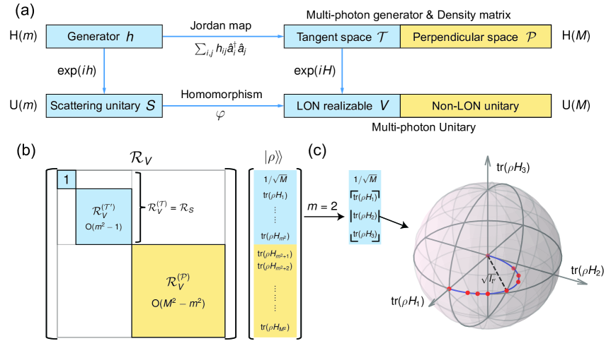
Figure 1: Theoretical framework of multi-photon linear optics. (a) The scattering unitary $S$ is mapped to the $n$-photon unitary $V$ via the homomorphism $\varphi$, which defines LON realizable unitaries within $\mathrm{U}(M)$ and distinguishes them from the non-LON ones. The generator $h$ of $S$ is connected to the $n$-photon generator $H$ through the JS map, forming the tangent space $\mathcal{T}$ within $\mathrm{H}(M)$, with the perpendicular space $\mathcal{P}$ as its orthogonal complement. (b) The HTM $\mathcal{R}_{V}$ exhibits a block-diagonal structure, $1\oplus\mathcal{R}_{V}^{(\mathcal{T^{\prime}})}\oplus\mathcal{R}_{V}^{(\mathcal{P})}$, which preserves the norms of the three density vector components and elucidates the origin of the different invariants. $\mathrm{O}(k)$ denotes the $k$-dimensional orthogonal group. (c) For the two-mode case ($m=2$), the density vector components in the traceless tangent space exhibit a spherical geometry (see SM Sec. IV & V [19]), with the invariant $I_{t^{\prime}}$ corresponding to the squared distance from the origin. The blue curve outlines the experimentally preparable states, while the red points indicate the eight states implemented in the experiment.

Theoretical framework—A lossless LON with $m$ modes can implement arbitrary unitary operations $S\in\mathrm{U}(m)$ [23, 24, 25, 26], termed scattering unitaries, where $\mathrm{U}(m)$ denotes the unitary group. For an $n$-photon input distributed across $m$ modes, the Fock basis states $\ket{\mathbf{n}}=\ket{n_{1},n_{2},\cdots,n_{m}}$ with $\sum_{i=1}^{m}n_{i}=n$, span an $M$-dimensional Fock space with $M=\binom{m+n-1}{n}$. This space encomprises all $n$-photon $m$-mode states (NMS), whose evolution is governed by an $M\times M$ $n$-photon unitary $V\in\mathrm{U}(M)$. This unitary is constructed via a photonic homomorphism $\varphi:\mathrm{U}(m)\mapsto\mathrm{U}(M)$ that depends on $S$ and $n$ through the matrix permanent [27, 12]. Since $M$ grows combinatorially with $n$, the parameter space of $\mathrm{U}(M)$ is exponentially larger than that of $\mathrm{U}(m)$. Consequently, $m$-mode LONs with $n$-photon inputs can only realize a subset of $\mathrm{U}(M)$ that is the image of $\varphi$ [16, 28, 29]. This effectively partitions $\mathrm{U}(M)$ into LON realizable unitaries $V\in\mathrm{Im}(\varphi)$ and those cannot.

The scattering unitary $S$ and its corresponding $n$-photon unitary $V$ are generated by the Hermitian operators $h\in\mathrm{H}(m)$ and $H\in\mathrm{H}(M)$, respectively, via $S=\exp(ih)$ and $V=\exp(iH)$, where $\mathrm{H}(k)$ denotes the space of $k\times k$ Hermitian matrices. The generators $h$ and $H$ are connected [30] by the Jordan-Schwinger (JS) map [31, 32], which introduces the second-quantized operator $\hat{O}=\sum_{i,j}h_{ij}\hat{a}_{i}^{\dagger}\hat{a}_{j}$, with $\hat{a}_{i}^{\dagger}$ and $\hat{a}_{j}$ representing the photon creation operator for mode $i$ and the annihilation operator for mode $j$, respectively. The normalized matrix representation of $\hat{O}$ in the $n$-photon, $m$-mode Fock basis $(\ket{\mathbf{n}})$ yields the $n$-photon generators $H$. Thus, the JS map partitions $\mathrm{H}(M)$ into two subspaces: the tangent space $\mathcal{T}$ of LON realizable generators and the perpendicular space $\mathcal{P}$ of non-LON generators, such that $\mathrm{H}(M)=\mathcal{T}\oplus\mathcal{P}$. This decomposition further highlights that only a subset of the unitaries in $\mathrm{U}(M)$ is LON realizable, as depicted in Fig. 1(a).

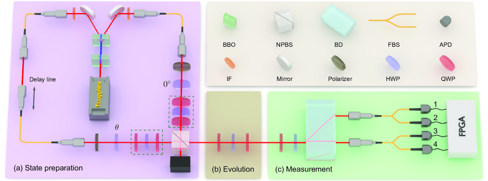
Figure 2: Experimental setup. (a) State Preparation: Photon pairs are generated via spontaneous parametric down-conversion and then pass through two interference filters (IFs). Two-photon states, $\ket{\psi_{\alpha}}=\cos\alpha\ket{2_{H},0}+\sin\alpha\ket{1_{H},1_{V}}$, with invariant values depending on $\alpha$, are prepared using Hong-Ou-Mandel interference followed by post-selection. The green dashed boxes highlight two groups of wave plates arranged in a QWP–HWP–QWP (QHQ) configuration, which correct for non-ideal phase and polarization changes induced by the non-polarizing beam splitter (NPBS) (see SM Sec. VII [19]). (b) Evolution: Arbitrary two-mode unitary evolutions are applied using an additional QHQ wave plate group. (c) Measurement: Projective measurements on two-photon two-mode bases are performed using a QWP and an HWP to set measurement bases, followed by a beam displacer (BD) and two pseudo photon-number-resolving detectors (PPNRDs). Each PPNRD comprises a fiber beam splitter (FBS) and two avalanche photodiodes (APDs), with detection counts processed by a field-programmable gate array (FPGA). BBO $\beta$-barium borate crystal. QWP quarter-wave plate. HWP half-wave plate.

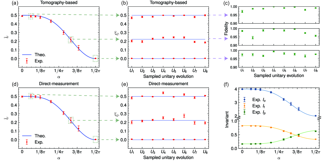
Figure 3: Experimental observation of invariants under LON unitaries. (a, d) Average experimental invariant $\bar{I}_{t^{\prime}}$ (red dots) for the input state $\ket{\psi_{\alpha}}$, defined as the mean of the measured values $I_{t^{\prime}}^{(k)}$ over eight distinct LON unitaries $U_{k}$, obtained by the tomography-based method (a) and by the direct-measurement method (d). Error bars denote the standard deviation of $\{I_{t^{\prime}}^{(k)}\}$. (b, e) Individual values $I_{t^{\prime}}^{(k)}$ for three exemplary input states under various unitaries, measured via the tomography-based method (b) and the direct-measurement method (e), with error bars given by a Poissonian distribution. (c) Tomography fidelities for the reconstructed states in (b). (f) Results of measured invariants $I_{o}$, $I_{t}$ and $I_{p}$. The theoretical values of different invariants are presented as lines.

To further elucidate this limitation, we introduce a specific basis for $\mathrm{H}(M)$ to reveal the structure of $V=\varphi(S)$. We begin with an orthonormal Hermitian basis for $\mathrm{H}(m)$:

$$\{h_{i}\}_{i=0}^{m^{2}-1}=\left\{\frac{I(m)}{\sqrt{m}},\lambda_{1}^{(m)},\lambda_{2}^{(m)},\dots,\lambda_{m^{2}-1}^{(m)}\right\},$$ (1)

which satisfies $\tr(h_{i}h_{j})=\delta_{ij}$. Here, $I(m)$ is the $m\times m$ identity matrix and $\{\lambda_{i}^{(m)}\}$ are the $m\times m$ generalized Gell-Mann matrices (see the Supplementary Material (SM) Sec. I  [19]). From $\{h_{i}\}$, the JS map produces the corresponding set of second-quantized operators $\{\hat{O}_{i}\}$, which naturally separate into four distinct classes $\{\hat{O}_{i}\}=\{\hat{O}_{0}^{(1)}\}\cup\{\hat{O}_{l}^{(2)}\}\cup\{\hat{O}_{jk}^{(3)}\}\cup\{\hat{O}_{jk}^{(4)}\}$: $\hat{O}_{0}^{(1)}=\sum_{j}^{m}\hat{n}_{j}/\sqrt{m}$, $\hat{O}_{l}^{(2)}=\sum_{j=1}^{l}(\hat{n}_{j}-\hat{n}_{l+1})/\sqrt{l(l+1)}$ for $l=1,\dots,m-1$, $\hat{O}_{jk}^{(3)}=\left(\hat{a}_{j}^{\dagger}\hat{a}_{k}+\hat{a}_{k}^{\dagger}\hat{a}_{j}\right)/{\sqrt{2}}$ and $\hat{O}_{jk}^{(4)}={i}\left(\hat{a}_{j}^{\dagger}\hat{a}_{k}-\hat{a}_{k}^{\dagger}\hat{a}_{j}\right)/{\sqrt{2}}$ for $1\leq j<k\leq m$, where $\hat{n}_{j}=\hat{a}_{j}^{\dagger}\hat{a}_{j}$ is the photon number operator for mode $j$. Let $\{O_{i}\}$ be the matrix representations of $\{\hat{O}_{i}\}$ in the $n$-photon, $m$-mode Fock basis. From the JS map, $\{O_{i}\}$ satisfy $\tr(O_{0}^{2})=n^{2}M/m$, $\tr(O_{i})=0$ and $\tr(O_{i}O_{j})=\binom{m+n}{m+1}\delta_{ij}$ for $i,j=1,\dots,m^{2}-1$ (see SM Sec. II [19]). This yields an orthonormal Hermitian basis for the subspace $\mathcal{T}$ as

$$H_{0}=\frac{O_{0}}{\sqrt{n^{2}M/m}},\ H_{i}=\frac{O_{i}}{\sqrt{\binom{m+n}{m+1}}}\ (i=1,\dots,m^{2}-1).$$ (2)

For the perpendicular space $\mathcal{P}$, an orthonormal and traceless basis $\{H_{i}\}_{i=m^{2}}^{M^{2}-1}$ is obtained via the Gram-Schmidt process. Together, $\{H_{i}\}_{i=0}^{M^{2}-1}$ forms a complete orthonormal basis for $\mathrm{H}(M)$, with $\{H_{i}\}_{i=1}^{M^{2}-1}$ being traceless.

Inspired by Pauli transfer matrix formalism [33, 34], we map a density matrix $\rho\in\mathrm{H}(M)$ of an NMS to a density vector $|\rho\rangle\!\rangle$ by expanding $\rho$ in the Hermitian basis $\{H_{i}\}$, where each $H_{i}$ corresponds to a basis vector $|i\rangle\!\rangle$. This yields $|\rho\rangle\!\rangle=\sum_{i}\langle\!\langle i|\rho\rangle\!\rangle|i\rangle\!\rangle$ with real coefficients $\langle\!\langle i|\rho\rangle\!\rangle=\tr(H_{i}\rho)$, and inner product defined as $\langle\!\langle A|B\rangle\!\rangle=\tr(A^{\dagger}B)$. Under an $n$-photon unitary $V=\varphi(S)$, the density vector evolves as $|V\rho V^{\dagger}\rangle\!\rangle=\mathcal{R}_{V}|\rho\rangle\!\rangle$, where the Hermitian transfer matrix (HTM) $\mathcal{R}_{V}$ acts as an orthogonal matrix with elements $(\mathcal{R}_{V})_{ij}=\tr(H_{i}VH_{j}V^{\dagger})$. Importantly, the two subspaces $\mathcal{T}$ and $\mathcal{P}$ of $\mathrm{H}(M)$ remain invariant under any LON realizable unitary $V$ [17], leading to the decomposition $\mathcal{R}_{V}=\mathcal{R}_{V}^{(\mathcal{T})}\oplus\mathcal{R}_{V}^{(\mathcal{P})}$ with $\mathcal{R}_{V}^{(\mathcal{T})}=\mathcal{R}_{S}$, where $\mathcal{R}_{S}$ is the HTM of the scattering unitary with $(\mathcal{R}_{S})_{ij}=\tr(h_{i}Sh_{j}S^{\dagger})$ (see SM Sec. III for proof [19]). $\mathcal{R}_{S}$ depends solely on the mode number $m$, reflecting single photon dynamics. In contrast, $\mathcal{R}_{V}^{(\mathcal{P})}$ grows exponentially with the photon number $n$, capturing the multi-photon interference effects induced by $S$. Any density vector can be decomposed as $|\rho\rangle\!\rangle=|\rho_{t}\rangle\!\rangle\oplus|\rho_{p}\rangle\!\rangle$, with $|\rho_{t}\rangle\!\rangle=\sum_{i=0}^{m^{2}-1}\tr(H_{i}\rho)|i\rangle\!\rangle$, $|\rho_{p}\rangle\!\rangle=\sum_{i=m^{2}}^{M^{2}-1}\tr(H_{i}\rho)|i\rangle\!\rangle$. Exploiting the block structure of $\mathcal{R}_{V}$, the norms of these components remain invariant, giving rise to the tangent and perpendicular invariants [17]:

$$I_{t} =\langle\!\langle\rho_{t}|\rho_{t}\rangle\!\rangle=\tr(\rho_{t}^{2})=\sum_{i=0}^{m^{2}-1}\tr(H_{i}\rho)^{2},$$ (3)

$$I_{p} =\langle\!\langle\rho_{p}|\rho_{p}\rangle\!\rangle=\tr(\rho_{p}^{2})=\sum_{i=m^{2}}^{M^{2}-1}\tr(H_{i}\rho)^{2}.$$ (4)

Since $\tr(H_{0}\rho)=\tr(\sum_{j}^{m}\hat{n}_{j}\rho)/n\sqrt{M}=1/\sqrt{M}$ holds for all NMS, the upper-left entry of $\mathcal{R}_{V}$ is fixed to unity. This further decomposes $\mathcal{R}_{V}$ as $\mathcal{R}_{V}=1\oplus\mathcal{R}^{(\mathcal{T}^{\prime})}_{V}\oplus\mathcal{R}_{V}^{(\mathcal{P})}$, as shown in Fig. 1(b). A photon number invariant $I_{n}=\tr(H_{0}\rho)^{2}=1/M$ emerges, reflecting the conservation of the total photon number. This block structure isolates the traceless tangent invariant

$$I_{t^{\prime}}=I_{t}-I_{n}=\sum_{i=1}^{m^{2}-1}\tr(H_{i}\rho)^{2},$$ (5)

separating it from the tangent invariant $I_{t}$. The sum of the invariants $I_{n}+I_{t^{\prime}}+I_{p}=\tr(\rho^{2})$ represents the state purity, and their conservation under LON unitary evolution implies that the purity contribution from each subspace remains invariant.

Experiments—We perform experiments to confirm that the invariants $I_{t^{\prime}}$, $I_{t}$ and $I_{p}$ remain conserved under LON unitary evolution. For an input NMS, we apply multiple different LON unitaries and extract the corresponding invariant values. To observe these invariants, we employ two approaches. First, a tomography-based method in which we reconstruct the full state using an $m$-mode LON and photon counting, and then calculate the values of $I_{t^{\prime}}$, $I_{t}$ and $I_{p}$ using Eq. (3)-(5). Yet, as $n$ and $m$ increase, the required number of distinct LON configurations for tomography $R_{n,m}=\binom{n+m}{n}-\binom{n+m-2}{m}$ grows combinatorially [35], rendering this method challenging for large systems. Instead, we can use the direct-measurement method to determine $I_{t^{\prime}}$ efficiently by measuring $m^{2}-1$ observables, $\{\hat{O}_{l}^{(2)}\},\{\hat{O}_{jk}^{(3)}\},\{\hat{O}_{jk}^{(4)}\}$, and calculating the invariant using Eq. (S13) and Eq. (5). The observables $\{\hat{O}_{l}^{(2)}\}$ are measured by photon counting after each mode, while $\{\hat{O}_{jk}^{(3)}\}$ and $\{\hat{O}_{jk}^{(4)}\}$ are measured through interference between modes $j$ and $k$ using a beam splitter, followed by photon counting on both output modes [36].

We demonstrate both tomography-based and direct-measurement methods for two-photon two-mode states using the setup in Fig. 2. The experimental platform comprise three modules: state preparation (a), evolution (b), and measurement (c). In the state preparation module, photon pairs are generated via type-II beam-like spontaneous parametric down-conversion pumped by a frequency-doubled Ti:sapphire laser. An HWP set at an angle $\theta$ prepares one photon in the superposition state $\cos 2\theta\ket{H}+\sin 2\theta\ket{V}$, where $\ket{H}$ and $\ket{V}$ denote horizontal and vertical polarizations, respectively, while the other photon is initialized in the $\ket{H}$ state. To produce two-photon states with distinct invariants that cannot be altered by unitary evolution alone, Hong-Ou-Mandel interference (HOMI) [37, 38] is performed at an NPBS, and events in which both photons exit a single output port are post-selected. This yields the state $\ket{\psi_{\alpha}}=\cos\alpha\ket{2_{H},0}+\sin\alpha\ket{1_{H},1_{V}}$ with $0\leq\alpha\leq\pi/2$, where $\alpha$ depends on $\theta$ (see SM Sec. VII [19]). In the traceless tangent space, the components of the density vector of $\ket{\psi_{\alpha}}$ trace a curve as a function of $\alpha$ with the invariant $I_{t^{\prime}}$ corresponding to the squared distance from the origin, as shown in Fig. 1(c). Eight distinct two-photon states are realized experimentally, as indicated by dots in Fig. 1(c).

In the evolution module, arbitrary linear optical unitary evolution on the two polarization modes are implemented using a QHQ wave plate group, comsisting of a half-wave plate (HWP) sandwiched between two quarter-wave plates (QWPs). In the measurement module, a beam displacer (BD) followed by two pseudo photon-number-resolving detectors (PPNRDs) enables projections onto the two-photon two-mode bases. Each PPNRD is realized by a FBS followed by two APDs. Coincidence events among the four APDs correspond to projections onto specific Fock states: {1, 2} for $\ket{2_{H},0_{V}}$; {1, 3}, {1, 4}, {2, 3} and {2, 4} for $\ket{1_{H},1_{V}}$; and {3, 4} for $\ket{0_{H},2_{V}}$. A QWP and an HWP positioned before the BD can be configured in various settings to enable projective measurements onto different states. Six distinct QWP–HWP settings in the measurement module facilitate quantum state tomography (QST) of the two-photon states [39, 35] (see the SM Sec. IX [19]). For each input state $\ket{\psi_{\alpha}}$, we apply eight distinct LON unitaries $U_{k}$ (see SM Sec. VIII [19]), yielding the measured invariants $I_{t^{\prime}}^{(k)}$ for $k=1,2,...,8$. Due to experimental uncertainties, these values may deviate slightly from the theoretical invariant $I_{t^{\prime}}$. Therefore, for each input state $\ket{\psi_{\alpha}}$, we define the average experimental invariant $\bar{I}_{t^{\prime}}$ as the mean of the measured values $\{I_{t^{\prime}}^{(k)}\}$.

Figure 3(a-b) present the invariants measured via the tomography‐based method. In Fig. 3(a), the average experimental invariant $\bar{I}_{t^{\prime}}$ closely agrees with the theoretical invariant $I_{t^{\prime}}$. Figure 3(b) shows the $I_{t^{\prime}}^{(k)}$ values for three representative input states under the sampled unitaries. The measured values consistently cluster around the theoretical invariant, demonstrating its conservation under LON unitary evolution, while the observed fluctuations reflect experimental errors. These deviations primarily stem from state preparation imperfections (e.g., limited HOMI visibility), measurement errors, and reconstruction errors introduced during QST. As shown in Fig. 3(c), the tomography fidelity of the evolved two-photon states, defined as $F=\left(\tr\sqrt{\rho^{1/2}\tilde{\rho}\rho^{1/2}}\right)^{2}$, quantifies the discrepancy between the experimentally reconstructed states $\tilde{\rho}$ and their theoretical counterparts $\rho$. States with lower fidelity exhibit larger deviations from the theoretical invariant values, indicating that experimental errors significantly contribute to these deviations. Finally, using the same reconstructed states, the measured values of $I_{t}$ and $I_{p}$ are shown in Fig. 3(f).

The direct-measurement method, which efficiently determines $I_{t^{\prime}}$ with only three measurement configurations, yields results shown in Fig. 3(d-e). In Fig. 3(d), the average experimental invariant $\bar{I}_{t^{\prime}}$ closely follow the theoretical prediction. In Fig. 3(e), the measured $I_{t^{\prime}}^{(k)}$ exhibit fluctuations around the theoretical line, comparable to or slightly more pronounced than those observed in the tomography-based results. This suggests that the direct-measurement method, which requires fewer measurement configurations and state copies, may be more susceptible to systematic errors.

In Ref. [18], a different invariant, referred to as the observable invariant $I_{o}$ here, was introduced based on a set of observables. In SM Sec. VI [19],we establish a connection between $I_{o}$ and $I_{t^{\prime}}$. In Fig. 3(f), we present the experimental result for observable invariant $I_{o}$ through direct-measurement approach.

Conclusion and outlook—In this work, we introduce Hermitian transfer matrix (HTM) as a new framework to investigate the unitary evolution of $n$-photon $m$-mode states. The block-diagonal structure of the HTM of an $n$-photon unitary clearly reveals the origin of multi-photon invariants and underscores the inherent limitations of linear optical evolution. Experimentally, we confirm the conservation of these invariants under unitary evolution in the two-photon two-mode case using both tomography-based and direct-measurement approaches. These findings establish HTM and invariants as powerful tools for exploring multi-photon linear optics. We expect that the HTM framework can be extended to general quantum processes for multi-photon states [40] and used to elucidate the limited expressivity of quantum photonic neural networks [41, 42], as well as applications in quantum sensing [43]. Moreover, the direct-measurement approach for invariants, requiring fewer measurements than full tomography, offers a promising tool for multi-photon state discrimination [44] and classification [29].

Note on Ref. [45]: Shortly before submission, we were aware of Rodari et al. [45], which also experimentally observed the invariant $I_{o}$, as well as the spectral invariant introduced in Ref. [18]. As mentioned in our work, $I_{o}$ is linearly related to $I_{t}^{\prime}$. While there is overlap, our purity‐like invariants differ in physical interpretation. The scalar invariants in Ref. [45] are given by the norm of the optical coherence matrix, where invariants in our work arise as the contributions of orthogonal subspaces to the total state purity.

Supplementary material: Experimental Observation of Purity-Like Invariants of Multiphoton States in Linear Optics

Appendix A I. Generalized Gell-Mann matrices

The Generalized Gell-Mann matrices (GGM) [20] generalize the Pauli matrices for qubits and the Gell-Mann matrices for qutrits to arbitrary dimensions. They form a complete basis for the space of $m\times m$ traceless Hermitian matrices.

Let $E_{jk}$ be the matrix with 1 in the $(j,k)$-th entry and 0 elsewhere. The GGM for a $m$-mode system are constructed as follows:

1. symmetric matrix: $\lambda_{i}^{(m)}=\frac{1}{\sqrt{2}}(E_{kj}+E_{jk}),\ k<j$

2. antisymmetric matrix: $\lambda_{i}^{(m)}=-\frac{i}{\sqrt{2}}\left(E_{kj}-E_{jk}\right),\ k>j$

3. diagonal matrix: $\lambda_{i}^{(m)}=\frac{1}{\sqrt{l(l+1)}}\left(\sum_{j=1}^{l}E_{jj}-lE_{l+1,l+1}\right),\ 1\leq l\leq m-1$

In this work, we adopt a convention where each GGM element is normalized by a factor of $1/\sqrt{2}$. Hence, unless otherwise specified, all references to GGM herein pertain to the normalized form.

The GGM exhibit the following fundamental properties:

• hermitian: $\left(\lambda_{i}^{(m)}\right)^{\dagger}=\lambda_{i}^{(m)}$.

• traceless: $\tr\left(\lambda_{i}^{(m)}\right)=0$.

• orthonormal: $\tr\left(\lambda_{i}^{(m)}\lambda_{j}^{(m)}\right)=\delta_{i,j}$.

In the case of 2-level systems, normalized Pauli matrices serve as the GGM:

$$\lambda_{1}^{(2)}=\frac{1}{\sqrt{2}}\begin{pmatrix}0&1\\ 1&0\end{pmatrix},\quad\lambda_{2}^{(2)}=\frac{1}{\sqrt{2}}\begin{pmatrix}0&-i\\ i&0\end{pmatrix},\quad\lambda_{3}^{(2)}=\frac{1}{\sqrt{2}}\begin{pmatrix}1&0\\ 0&-1\end{pmatrix}.$$ (S1)

In the case of 3-level system, normalized Gell-Mann matrices serve as the GGM:

$$\lambda_{1}^{(3)}=\frac{1}{\sqrt{2}}\begin{pmatrix}0&1&0\\ 1&0&0\\ 0&0&0\end{pmatrix},\quad\lambda_{2}^{(3)}=\frac{1}{\sqrt{2}}\begin{pmatrix}0&-i&0\\ i&0&0\\ 0&0&0\end{pmatrix},\quad\lambda_{3}^{(3)}=\frac{1}{\sqrt{2}}\begin{pmatrix}1&0&0\\ 0&-1&0\\ 0&0&0\end{pmatrix},$$ (S2)

$$\lambda_{4}^{(3)}=\frac{1}{\sqrt{2}}\begin{pmatrix}0&0&1\\ 0&0&0\\ 1&0&0\end{pmatrix},\quad\lambda_{5}^{(3)}=\frac{1}{\sqrt{2}}\begin{pmatrix}0&0&-i\\ 0&0&0\\ i&0&0\end{pmatrix},$$

$$\lambda_{6}^{(3)}=\frac{1}{\sqrt{2}}\begin{pmatrix}0&0&0\\ 0&0&1\\ 0&1&0\end{pmatrix},\quad\lambda_{7}^{(3)}=\frac{1}{\sqrt{2}}\begin{pmatrix}0&0&0\\ 0&0&-i\\ 0&i&0\end{pmatrix},\quad\lambda_{8}^{(3)}=\frac{1}{\sqrt{6}}\begin{pmatrix}1&0&0\\ 0&1&0\\ 0&0&-2\end{pmatrix}.$$

Appendix B II. Jordan-Schwinger map connect two Hermitian space

The Jordan-Schwinger (JS) map [31, 32, 30] is defined as:

$$h_{i}\longmapsto\hat{O}_{i}\equiv\sum_{k,l}\hat{a}_{k}^{\dagger}(h_{i})_{kl}\hat{a}_{l}.$$ (S3)

The JS map connects the generator of scattering matrix $h_{i}\in\mathrm{H}(m)$ to the generator of multiphoton unitary $H_{i}\in\mathrm{H}(M)$. In this section, we prove that for the Hermitian basis $\{h_{i}\}$ given by (Eq. (1) in the main text):

$$\{h_{i}\}_{i=0}^{m^{2}-1}=\left\{\frac{I(m)}{\sqrt{m}},\lambda_{1}^{(m)},\lambda_{2}^{(m)},\dots,\lambda_{m^{2}-1}^{(m)}\right\},$$ (S4)

the set of observable $\{\hat{O}_{i}\}$—the image of $\{h_{i}\}$ under the JS map—are orthogonal.

In the following derivation, we donate by $O_{i}$ the matrix representation of $\hat{O}_{i}$ in the $n$-photon $m$-mode Fock basis, with entries defined as $(O_{i})_{jk}=\innerproduct{\mathbf{n}_{j}\left|\hat{O}\right|\mathbf{n}_{k}}{\mathbf{n}_{j}\left|\hat{O}\right|\mathbf{n}_{k}}$. The Fock basis states are given by $\ket{\mathbf{n}}=\ket{n_{1},n_{2},\cdots,n_{m}}$ with $\sum_{i=1}^{m}n_{i}=n$, spanning an $M$-dimensional Hilbert space with $M=\binom{m+n-1}{n}$. Additionally, for any operator $\tr(\hat{A})$, the trace $\tr(\hat{A})$ in the Fock basis is given by $\tr(\hat{A})=\sum_{i=1}^{M}\innerproduct{\mathbf{n}_{i}\left|\hat{A}\right|\mathbf{n}_{i}}{\mathbf{n}_{i}\left|\hat{A}\right|\mathbf{n}_{i}}$.

For $n$-photon $m$-mode states (NMS), the following trace relations of photon number operator will be used in the proof:

$$\tr\left(\hat{n}_{i}\right)=\sum_{i=0}^{n}i\binom{m-2+n-i}{m-2}=\binom{m+n-1}{m},$$ (S5)

$$\tr\left(\hat{n}_{i}\hat{n}_{j}\right)=\sum_{i=0}^{n}\left[\left(\sum_{j=0}^{i}j(i-j)\right)\binom{m-3+n-i}{m-3}\right]=\binom{m+n-1}{m+1},\quad i\neq j$$ (S6)

$$\begin{aligned} \tr\left(\hat{n}_{i}^{2}\right)=\sum_{i=0}i^{2}\binom{m-2+n-i}{m-2}&=(1-m+2n)\frac{(m+n-1)!}{(m+1)!(n-1)!}\\ &=\binom{m+n-1}{m+1}+\binom{m+n}{m+1}.\\ \end{aligned}$$ (S7)

Theorem 1.

Under the JS map, the GGM for $m$-mode system $\{\lambda_{i}^{(m)}\}$ are mapped to a set of matrices $\{O_{i}\}_{i=1}^{m^{2}-1}$, which preserve the following properties of GGM:

• hermitian: $O_{i}^{\dagger}=O_{i}$.

• traceless: $\tr(O_{i})=0$.

• orthogonal: $\tr(O_{i}O_{j})=\binom{m+n}{m+1}\delta_{i,j}$.

Proof.

Hermitian:

$$\hat{O}_{i}^{\dagger} =\left(\sum_{k,l}\hat{a}_{k}^{\dagger}\left(\lambda_{i}^{(m)}\right)_{kl}\hat{a}_{l}\right)^{\dagger}$$ (S8)

$$=\sum_{k,l}\hat{a}_{l}^{\dagger}\left(\lambda_{i}^{(m)}\right)_{kl}^{*}\hat{a}_{k}$$

$$=\sum_{l,k}\hat{a}_{k}^{\dagger}\left(\lambda_{i}^{(m)}\right)_{lk}^{*}\hat{a}_{l}$$

$$=\sum_{l,k}\hat{a}_{k}^{\dagger}\left(\lambda_{i}^{(m)}\right)_{kl}\hat{a}_{l}$$

$$=\hat{O}_{i}.$$

Thus, $O_{i}^{\dagger}=O_{i}$.

Traceless:

$$\tr(O_{i}) =\sum_{k,l}\left(\lambda_{i}^{(m)}\right)_{kl}\tr\left(\hat{a}_{k}^{\dagger}\hat{a}_{l}\right)$$ (S9)

$$=\sum_{k}\left(\lambda_{i}^{(m)}\right)_{kk}\tr\left(\hat{a}_{k}^{\dagger}\hat{a}_{k}\right)$$

$$=\sum_{k}\left(\lambda_{i}^{(m)}\right)_{kk}\tr\left(\hat{n}_{k}\right)$$

$$=\tr\left(\lambda_{i}^{(m)}\right)\binom{m+n-1}{m}$$

$$=0.$$

Orthogonal:

$$\tr(O_{i}O_{j}) =\sum_{k,l,s,t}\left(\lambda_{i}^{(m)}\right)_{kl}\left(\lambda_{j}^{(m)}\right)_{st}\tr\left(\hat{a}^{\dagger}_{k}\hat{a}_{l}\hat{a}^{\dagger}_{s}\hat{a}_{t}\right)$$ (S10)

$$=\binom{m+n-1}{m+1}\left[\tr\left(\lambda_{i}^{(m)}\right)\tr\left(\lambda_{j}^{(m)}\right)-\sum_{k}\left(\lambda_{i}^{(m)}\right)_{kk}\left(\lambda_{j}^{(m)}\right)_{kk}\right] \quad(k=l,s=t,k\neq t)$$

$$+\binom{m+n}{m+1}\left[\tr\left(\lambda_{i}^{(m)}\lambda_{j}^{(m)}\right)-\sum_{k}\left(\lambda_{i}^{(m)}\right)_{kk}\left(\lambda_{j}^{(m)}\right)_{kk}\right] \quad(k=t,l=s,k\neq l)$$

$$+\left[\binom{m+n-1}{m+1}+\binom{m+n}{m+1}\right]\sum_{k}\left(\lambda_{i}^{(m)}\right)_{kk}\left(\lambda_{j}^{(m)}\right)_{kk} \quad(k=l=s=t)$$

$$=\binom{m+n}{m+1}\tr\left(\lambda_{i}^{(m)}\lambda_{j}^{(m)}\right)$$

$$=\binom{m+n}{m+1}\delta_{i,j}.$$

∎

The GGMs are orthogonal with identity matrix. For $m$-dimensional Hermitian, the normalized identity matrix is $h_{0}=I(m)/\sqrt{m}$, where $I(d)$ denotes $d$-dimensional identity matrix. Under the JS map, the image of $h_{0}$ is $O_{0}=\frac{n}{\sqrt{m}}I(M)$, with $\tr(O_{0}^{2})=\frac{n^{2}}{m}M=\frac{n^{2}}{m}\binom{m+n-1}{n}$.

Thus, if we choose hermitian basis as given in Eq. (S4), the corresponding observables $\{\hat{O}_{i}\}_{i=0}^{m^{2}-1}$ naturally separate into four distinct classes $\{\hat{O}_{i}\}=\{\hat{O}_{0}^{(1)}\}\cup\{\hat{O}_{l}^{(2)}\}\cup\{\hat{O}_{jk}^{(3)}\}\cup\{\hat{O}_{jk}^{(4)}\}$:

$$\hat{O}_{0}^{(1)} =\sum_{j}^{m}\hat{n}_{j}/\sqrt{m},$$ (S11)

$$\hat{O}_{l}^{(2)} =\sum_{j=1}^{l}(\hat{n}_{j}-\hat{n}_{l+1})/\sqrt{l(l+1)}\quad \quad l=1,\dots,m-1,$$

$$\hat{O}_{jk}^{(3)} =\left(\hat{a}_{j}^{\dagger}\hat{a}_{k}+\hat{a}_{k}^{\dagger}\hat{a}_{j}\right)/\sqrt{2}\quad \quad 1\leq j<k\leq m,$$

$$\hat{O}_{jk}^{(4)} =i\left(\hat{a}_{j}^{\dagger}\hat{a}_{k}-\hat{a}_{k}^{\dagger}\hat{a}_{j}\right)/\sqrt{2}\quad \quad 1\leq j<k\leq m.$$

And the orthonormality condition can be summarized as follows:

$$\tr(O_{i}O_{j})=\binom{m+n}{m+1}\delta_{i,j}\quad\text{except for}\quad\tr(O_{0}^{2})=\frac{n^{2}}{m}M.$$ (S12)

From this, we construct the orthonormal hermitian basis $\{H_{i}\}_{i=0}^{m^{2}-1}$ for tangent space $\mathcal{T}$ by normalizing $\{O_{i}\}_{i=0}^{m^{2}-1}$ (Eq. (2) of the main text):

$$H_{0}=\frac{O_{0}}{\sqrt{n^{2}M/m}},\ H_{i}=\frac{O_{i}}{\sqrt{\binom{m+n}{m+1}}}\ (i=1,\dots,m^{2}-1).$$ (S13)

For the perpendicular space $\mathcal{P}$, a set of orthonormal and traceless bases as $\{H_{i}\}_{i=m^{2}}^{M^{2}-1}$ can be obtain by applying the Gram-Schmidt process [17]. Together, $\{H_{i}\}_{i=0}^{M^{2}-1}$ forms a complete orthonormal basis for $\mathrm{H}(M)$ with $\{H_{i}\}_{i=1}^{M^{2}-1}$ being traceless.

Appendix C III. Properties of the Hermitian Transfer Matrix

Hermitian Transfer Matrix (HTM) describes the evolution of a density vector—specifically, the vectorized density matrix defined in hermitian basis for the generator of multiphoton unitary $\{H_{i}\}_{i=0}^{M^{2}-1}$ given in Eq. (S13)—under a linear optical network (LON). In this section, we first introduce the motivation behind defining the HTM, followed by an exploration of its key properties.

Consider the evolution of the density vector under a LON realizable multi-photon unitary $V$:

$$|V\rho V^{\dagger}\rangle\!\rangle =\sum_{i}|i\rangle\!\rangle\langle\!\langle i|V\rho V^{\dagger}\rangle\!\rangle$$ (S14)

$$=\sum_{i}|i\rangle\!\rangle\tr(H_{i}V\rho V^{\dagger})$$

$$=\sum_{i,j}|i\rangle\!\rangle\tr(H_{i}VH_{j}V^{\dagger})\tr(H_{j}\rho)$$

$$=\left[\sum_{i,j}|i\rangle\!\rangle\tr(H_{i}VH_{j}V^{\dagger})\langle\!\langle j|\right]|\rho\rangle\!\rangle$$

$$=\mathcal{R}_{V}|\rho\rangle\!\rangle,$$

where the HTM is defined as $(\mathcal{R}_{V})_{ij}=\langle\!\langle i|\mathcal{R}_{V}|j\rangle\!\rangle=\tr(H_{i}VH_{j}V^{\dagger})$.

The HTM exhibits several notable properties due to the constraints of LONs and our choice of multi-photon generator basis.

1. Reality: The entries of $\mathcal{R}_{V}$ are real as:

$$\tr(H_{i}VH_{j}V^{\dagger})^{\dagger}=\tr(VH_{j}V^{\dagger}H_{i})=\tr(H_{i}VH_{j}V^{\dagger}).$$ (S15)

2. Orthogonality: The matrix $\mathcal{R}_{V}$ is orthogonal. Using the Hilbert-Schmidt inner product:

$$\langle\!\langle V^{\dagger}H_{i}V|V^{\dagger}H_{j}V\rangle\!\rangle =\sum_{k}\langle\!\langle V^{\dagger}H_{i}V|k\rangle\!\rangle\langle\!\langle k|V^{\dagger}H_{j}V\rangle\!\rangle$$ (S16)

$$=\sum_{k}\tr(H_{k}V^{\dagger}H_{i}V)\tr(H_{k}V^{\dagger}H_{j}V)$$

$$=\sum_{k}(\mathcal{R}_{V})_{ki}(\mathcal{R}_{V})_{kj}.$$

Meanwhile, the orthonormality of $\{H_{i}\}$ gives:

$$\langle\!\langle V^{\dagger}H_{i}V|V^{\dagger}H_{j}V\rangle\!\rangle=\tr(H_{i}H_{j})=\delta_{ij}.$$ (S17)

Equating the two expressions, we find:

$$\sum_{k}(\mathcal{R}_{V})_{ki}(\mathcal{R}_{V})_{kj}=\delta_{ij},$$ (S18)

which confirms that $\mathcal{R}_{V}$ is orthogonal.

3. Block-Diagonality: Due to the limited degrees of freedom $m^{2}$ in a LON, $\mathcal{R}_{V}$ cannot fully achieve the orthogonal group $\mathrm{O}(M^{2})$. However, the invariance of the tangent $\mathcal{T}$ and perpendicular $\mathcal{P}$ spaces—i.e., $V^{\dagger}H_{i}V\in\mathcal{T}$ if and only if $H_{i}\in\mathcal{T}$, and likewise for $\mathcal{P}$—ensures that $\mathcal{R}_{V}$ is block-diagonal:

$$(\mathcal{R}_{V})_{ij}=\tr(H_{i}VH_{j}V^{\dagger})=0,\quad\text{for }H_{i}\in\mathcal{T},\,H_{j}\in\mathcal{P}\text{ or vice versa}.$$ (S19)

From this we obtain the decomposition $\mathcal{R}_{V}=\mathcal{R}_{V}^{(\mathcal{T})}\oplus\mathcal{R}_{V}^{(\mathcal{P})}$ where $\mathcal{R}_{V}^{(\mathcal{T})}$ and $\mathcal{R}_{V}^{(\mathcal{P})}$ correspond to the upper-left and lower-right block-diagonal parts of $\mathcal{R}_{V}$, acting on the tangent space and the perpendicular space, respectively.

4. Equivalence of $\mathcal{R}_{V}^{(\mathcal{T})}$ and $\mathcal{R}_{S}$ The matrix $\mathcal{R}_{S}$ represent the HTM of scattering matrix, define in the hermitian basis $\{h_{i}\}$ with entries given by $(\mathcal{R}_{S})_{ij}=\tr(h_{i}Sh_{j}S^{\dagger})$. The following derivation relies on the adjoint representation and the consistency condition for Lie algebra homomorphisms from the group theory.

Consider a Lie group element $S\in\mathrm{U}(m)$, representing the scattering matrix. The adjoint representation acts on the Lie algebra $h\in\mathrm{H}(m)$ as:

$$\operatorname{Ad}_{S}(h)=ShS^{\dagger},$$ (S20)

which defines an automorphism of the Lie algebra.

Since the JS map, donated by $d\varphi$, is a Lie algebra homomorphism, it must satisfy the consistency condition [21]:

$$d\varphi(\mathrm{Ad}_{S}(h_{i}))=\mathrm{Ad}_{\varphi(S)}(d\varphi(h_{i})),$$ (S21)

which ensures that the mapping $d\varphi$ respects the evolution properties under the adjoint action. Expanding this relation explicitly, we obtain:

$$VO_{j}V^{\dagger}=\varphi(S)d\varphi(h_{j})\varphi(S)^{\dagger}=d\varphi(Sh_{j}S^{\dagger}).$$ (S22)

According to the normalization factor given in Eq. (S12), we also have:

$$\tr(d\varphi(h_{i})d\varphi(h_{j}))=\tr(O_{i}O_{j})=\binom{m+n}{m+1}\delta_{ij}.$$ (S23)

Combining these properties, we directly compute $\mathcal{R}_{V}$ entries for $0<i,j<m^{2}$:

$$(\mathcal{R}_{V})_{ij} =\tr\left(H_{i}VH_{j}V^{\dagger}\right)$$ (S24)

$$=\frac{1}{\binom{m+n}{m+1}}\tr\left(O_{i}VO_{j}U^{\dagger}\right)\quad\text{(normalization factor)}$$

$$=\frac{1}{\binom{m+n}{m+1}}\tr\big(d\varphi(h_{i})\cdot d\varphi(Sh_{j}S^{\dagger})\big{missing})\quad\text{(adjoint action)}$$

$$=\frac{1}{\binom{m+n}{m+1}}\tr\left(d\varphi(h_{i})d\varphi\left(\sum_{k}\tr(h_{k}Sh_{j}S^{\dagger})h_{k}\right)\right)\quad\text{(expand $Sh_{j}S^{\dagger}$ in $\{h_{k}\}$)}$$

$$=\frac{1}{\binom{m+n}{m+1}}\sum_{k}(\mathcal{R}_{S})_{kj}\tr(d\varphi(h_{i})d\varphi(h_{k}))$$

$$=\sum_{k}(\mathcal{R}_{S})_{kj}\delta_{ik}\quad\text{(orthonormality)}$$

$$=(\mathcal{R}_{S})_{ij}.$$

For the entries where $i=0$ or $j=0$, we can prove that $(\mathcal{R}_{V})_{ij}=(\mathcal{R}_{S})_{ij}=\delta_{ij}$. The proof follows the same reasoning as the following part. Thus $\mathcal{R}_{V}=\mathcal{R}_{S}\oplus\mathcal{R}_{V}^{(\mathcal{P})}$

5. Further Block-Diagonality: Within tangent space $\mathcal{T}$, the basis element $H_{0}=I(M)/\sqrt{M}$ is the only non-traceless operator. For any multiphoton quantum state $\rho$,

$$\langle\!\langle 0|\rho\rangle\!\rangle=\tr(\rho H_{0})=\frac{1}{\sqrt{M}}\tr(\rho)=\frac{1}{\sqrt{M}}.$$ (S25)

This implies that $\mathcal{R}_{V}$ acts as the identity on $|0\rangle\!\rangle$. The entries

$$(\mathcal{R}_{V})_{0j}=\tr(H_{0}U^{\dagger}H_{j}U)=\tr(H_{j})/\sqrt{M}=\delta_{0j},$$ (S26)

$$(\mathcal{R}_{V})_{i0}=\tr(H_{i}U^{\dagger}H_{0}U)=\tr(H_{i})/\sqrt{M}=\delta_{i0},$$ (S27)

indicate that $\mathcal{R}_{V}$ can be further block-diagonalized as $\mathcal{R}_{V}=1\oplus\mathcal{R}^{(\mathcal{T}^{\prime})}_{V}\oplus\mathcal{R}_{V}^{(\mathcal{P})}$. Where $\mathcal{T}^{\prime}$ donates the traceless tangent space, and $\mathcal{R}^{(\mathcal{T}^{\prime})}$ donate the lower-right block of $\mathcal{R}_{S}$, acting on the traceless tangent space $\mathcal{T}^{\prime}$. The block-diagonal form of $\mathcal{R}_{V}$ is depicted in Fig. 1(b) of the main text.

The block-diagonal form of the orthogonal matrix $\mathcal{R}_{V}$ preserve the vector norms within each subspace, allowing us to define the photon-number invariant $I_{n}=\tr^{2}(H_{0}\rho)$, the traceless tangent invariant $I_{t^{\prime}}=\sum_{i=1}^{m^{2}-1}\tr^{2}(H_{i}\rho)$, and the perpendicular invariant $I_{p}=\sum_{i=m^{2}}^{M^{2}}\tr^{2}(H_{i}\rho)$.

Based on the above analysis, we can represent a multi-photon state as two vectors, one in the traceless tangent space of dimension $m^{2}-1$ and the other in the perpendicular space of dimension $M^{2}-m^{2}$. The evolution of multi-photon state corresponds to distinct rotations applied to these two vectors. The necessary and sufficient condition for two multi-photon state to evolve into each other is the existence of a scattering unitary $S$ such that the initial state’s vectors, after rotation, coincide with the final state’s vectors in both spaces.

However, from the perspective of degrees of freedom, such a scattering unitary $S$ does not always exist. A LON with $m$ modes corresponds to an $m$-dimensional scattering unitary with $m^{2}$ degrees of freedom. On the other hand, the orthogonal group $\mathrm{O}(m^{2}-1)$ has $(m^{2}-1)(m^{2}-2)/2$ degrees of freedom. For $m>2$, it is impossible for the scattering unitary $S$ to generate arbitrary evolutions in $\mathrm{O}(m^{2}-1)$. Consequently, even in the traceless tangent space, we cannot always align two arbitrary vectors of the same length.

The sum of the invariants $I_{n}+I_{t^{\prime}}+I_{p}=\tr(\rho^{2})$ represents the state purity, and their conservation under LON unitary evolution implies that the purity contribution from each subspace remains invariant.

Appendix D IV. Hermitian Transfer Matrix in the two-photon, two-mode case

In this section, we derive the explicit expression of the $\mathcal{R}_{V}$ for the two-photon, two-mode case step by step.

As defined in Eq. (S11) the observables for the two mode case (m=2) are given by:

$$\hat{O}_{0} =\frac{1}{\sqrt{2}}\left(\hat{n}_{1}+\hat{n}_{2}\right),$$ (S28)

$$\hat{O}_{1} =\frac{1}{\sqrt{2}}\left(\hat{n}_{1}-\hat{n}_{2}\right),$$

$$\hat{O}_{2} =\frac{1}{\sqrt{2}}\left(\hat{a}_{1}^{\dagger}\hat{a}_{2}+\hat{a}_{1}\hat{a}_{2}^{\dagger}\right),$$

$$\hat{O}_{3} =\frac{i}{\sqrt{2}}\left(\hat{a}_{1}^{\dagger}\hat{a}_{2}-\hat{a}_{1}\hat{a}_{2}^{\dagger}\right).$$

Next, we derive the matrix representation $\{O_{i}\}$ of the operators $\{\hat{O}_{i}\}$ in the 2-photon 2-mode Fock basis, given by $\{\ket{\mathbf{n}_{i}}\}=\{\ket{0,2},\ket{1,1},\ket{2,0}\}$. Using the orthonormal relation given in Eq. (S12), we normalize ${O_{i}}$ as follows:

$$H_{0}=\frac{1}{\sqrt{6}}O_{0},\quad H_{i}=\frac{1}{2}O_{i}\quad(1\leq i\leq 3).$$ (S29)

The exact form of $\{H_{i}\}_{i=0}^{3}$ are given by:

$$H_{0} =\begin{pmatrix}\frac{1}{\sqrt{3}}&0&0\\ 0&\frac{1}{\sqrt{3}}&0\\ 0&0&\frac{1}{\sqrt{3}}\\ \end{pmatrix},H_{1}=\begin{pmatrix}\frac{1}{\sqrt{2}}&0&0\\ 0&0&0\\ 0&0&-\frac{1}{\sqrt{2}}\\ \end{pmatrix},H_{2}=\begin{pmatrix}0&\frac{1}{2}&0\\ \frac{1}{2}&0&\frac{1}{2}\\ 0&\frac{1}{2}&0\\ \end{pmatrix},H_{3}=\begin{pmatrix}0&-\frac{i}{2}&0\\ \frac{i}{2}&0&-\frac{i}{2}\\ 0&\frac{i}{2}&0\\ \end{pmatrix}.$$ (S30)

Using Schmidt orthogonalization, we construct the basis for the perpendicular space:

$$H_{4} =\begin{pmatrix}\frac{1}{\sqrt{6}}&0&0\\ 0&-\sqrt{\frac{2}{3}}&0\\ 0&0&\frac{1}{\sqrt{6}}\\ \end{pmatrix},H_{5}=\begin{pmatrix}0&\frac{1}{2}&0\\ \frac{1}{2}&0&-\frac{1}{2}\\ 0&-\frac{1}{2}&0\\ \end{pmatrix},H_{6}=\begin{pmatrix}0&-\frac{i}{2}&0\\ \frac{i}{2}&0&\frac{i}{2}\\ 0&-\frac{i}{2}&0\\ \end{pmatrix},H_{7}=\begin{pmatrix}0&0&-\frac{i}{\sqrt{2}}\\ 0&0&0\\ \frac{i}{\sqrt{2}}&0&0\\ \end{pmatrix},$$ (S31)

$$H_{8} =\begin{pmatrix}0&0&\frac{1}{\sqrt{2}}\\ 0&0&0\\ \frac{1}{\sqrt{2}}&0&0\\ \end{pmatrix}.$$

The scattering matrix for a two-mode LON is parameterized as:

$$S=\begin{pmatrix}e^{\frac{i}{2}(\alpha+\gamma)}\cos\left(\frac{\beta}{2}\right)&e^{\frac{i}{2}(\alpha-\gamma)}\sin\left(\frac{\beta}{2}\right)\\ -e^{-\frac{i}{2}(\alpha-\gamma)}\sin\left(\frac{\beta}{2}\right)&e^{-\frac{i}{2}(\alpha+\gamma)}\cos\left(\frac{\beta}{2}\right)\\ \end{pmatrix}.$$ (S32)

We briefly discuss the calculation of the photonic homomorphism $\varphi$ as detailed in Ref. [12]. Consider an $m$-mode LON with a scattering matrix $S$. Let $\ket{A}=\ket{a_{1},\dots,a_{m}}$ denote the input state and $\ket{B}=\ket{b_{1},\dots,b_{m}}$ the target state. The probability amplitude of obtaining the state $\ket{B}$ when the input is $\ket{A}$ is given by $\innerproduct{B|\varphi(S)|A}{B|\varphi(S)|A}$. According to Ref. [12], this amplitude is expressed as:

$$\innerproduct{B|\varphi(S)|A}{B|\varphi(S)|A}=\frac{\operatorname{Per}(S_{B,A})}{\sqrt{b_{1}!\cdots b_{m}!\,a_{1}!\cdots a_{m}!}}$$ (S33)

Here, $S_{B,A}$ is constructed by first selecting the $i$-th column of $S$ $a_{i}$ times to form the matrix $S_{A}$, and then selecting the $j$-th row of $S_{A}$ $b_{j}$ times to obtain $S_{B,A}$. The function $\operatorname{Per}(\cdot)$ denotes the permanent of the matrix.

Through the photonic homomorphism $\varphi$, the corresponding multiphoton unitary $V$ is:

$$V=\begin{pmatrix}e^{i(\alpha+\gamma)}\cos^{2}\left(\frac{\beta}{2}\right)&\sqrt{2}e^{i\alpha}\sin\left(\frac{\beta}{2}\right)\cos\left(\frac{\beta}{2}\right)&e^{i(\alpha-\gamma)}\sin^{2}\left(\frac{\beta}{2}\right)\\ -\sqrt{2}e^{i(\gamma-\alpha)}\sin\left(\frac{\beta}{2}\right)\cos\left(\frac{\beta}{2}\right)&\cos^{2}\left(\frac{\beta}{2}\right)-\sin^{2}\left(\frac{\beta}{2}\right)&\sqrt{2}e^{-i(\alpha-\gamma)}\sin\left(\frac{\beta}{2}\right)\cos\left(\frac{\beta}{2}\right)\\ e^{-i(\alpha-\gamma)}\sin^{2}\left(\frac{\beta}{2}\right)&-\sqrt{2}e^{-i\alpha}\sin\left(\frac{\beta}{2}\right)\cos\left(\frac{\beta}{2}\right)&e^{-i(\alpha+\gamma)}\cos^{2}\left(\frac{\beta}{2}\right)\\ \end{pmatrix}.$$ (S34)

Using the definition $(\mathcal{R}_{V})_{ij}=\tr(H_{i}VH_{j}V^{\dagger})$, the HTM block $\mathcal{R}_{V}^{(\mathcal{T})}$, or equivalently $\mathcal{R}_{S}$, is given by:

$$\mathcal{R}_{V}^{(\mathcal{T})}=\mathcal{R}_{S}=\begin{pmatrix}1&0&0&0\\ 0&\cos(\beta)&\sin(\beta)\cos(\gamma)&\sin(\beta)\sin(\gamma)\\ 0&-\cos(\alpha)\sin(\beta)&\cos(\alpha)\cos(\beta)\cos(\gamma)-\sin(\alpha)\sin(\gamma)&\cos(\alpha)\cos(\beta)\sin(\gamma)+\sin(\alpha)\cos(\gamma)\\ 0&\sin(\alpha)\sin(\beta)&-\sin(\alpha)\cos(\beta)\cos(\gamma)-\cos(\alpha)\sin(\gamma)&\cos(\alpha)\cos(\gamma)-\sin(\alpha)\cos(\beta)\sin(\gamma)\\ \end{pmatrix}.$$ (S35)

The $\mathcal{R}_{V}^{(\mathcal{T}^{\prime})}$ block acting on traceless tangent space corresponds to the canonical 2-to-1 homomorphism from $\mathrm{SU}(2)$ to $\mathrm{SO}(3)$, which means the $\mathcal{R}_{V}^{(\mathcal{T}^{\prime})}$ block can take any element in the orthogonal group $\mathrm{SO}(3)$ in the two-mode case.

Appendix E V. Range of traceless tangent invariant in the Two-Mode Case

In this section, we give the range of traceless tangent invariant in the two-mode case. In the two-mode case, as $\mathcal{R}_{V}^{(\mathcal{T}^{\prime})}$ can take any element in the orthogonal group $\mathrm{SO}(3)$, the density vector components in the traceless tangent space $\big{(}\tr(\rho H_{1}),\tr(\rho H_{2}),\tr(\rho H_{2})\big{)}$ form a spherical geometry as depicted in Fig. 1(c) of the main text. Therefore, the global maximum of $I_{t^{\prime}}$ can be determined by finding the maximum value along a specific axis.

Using the observables for two modes as given in Eq. (S28), and normalization factors from Eq. (S12), the invariant $I_{t^{\prime}}$ is expressed as:

$$I_{t^{\prime}}=\sum_{i=1}^{3}\tr^{2}(\rho H_{i})=\frac{1}{\binom{n+2}{3}}\sum_{i=1}^{3}\tr^{2}(\rho\hat{O}_{i}).$$ (S36)

To find the maximum value of $I_{t^{\prime}}$, we consider the state $\rho_{a}=\ket{n,0}\!\!\bra{n,0}$. For this state, the expectation values of the traceless tangent observables are:

$$\tr(\rho_{a}\hat{O}_{1})=\frac{1}{\sqrt{2}}\tr\big(\rho_{a}(\hat{n}_{1}-\hat{n}_{2})\big{missing})=\frac{n}{\sqrt{2}},\tr(\rho_{a}\hat{O}_{2})=\tr(\rho_{a}\hat{O}_{3})=0.\quad$$ (S37)

The corresponding expectation values along each axis are:

$$\tr(\rho_{a}H_{1})=\frac{n}{\sqrt{2\binom{n+2}{3}}}=\sqrt{\frac{3n}{(n+1)(n+2)}},\quad\tr(\rho_{a}H_{2})=\tr(\rho_{a}H_{3})=0.\quad$$ (S38)

Since $\rho_{a}$ maximizes the invariant value along the $H_{1}$ axis, it yields the global maximum of $I_{t^{\prime}}$:

$$I_{t^{\prime},\text{max}}=\frac{3n}{(n+1)(n+2)}.$$ (S39)

In Fig. 1(c) of the main text, the state $\rho_{\text{max}}$ corresponds to the apex of the sphere.

To determine the minimum value of $I_{t^{\prime}}$, we consider the state $\rho_{b}=I(M)/M$, representing an equal mixture of Fock basis states. For this state, $\tr(\rho_{b}H_{i})=\frac{1}{M}\tr(H_{i})=0$ for all $i=1,2,3$. Thus, the minimum value of $I_{t^{\prime}}$ is:

$$I_{t^{\prime},\text{min}}=0.$$ (S40)

In conclusion, the range of $I_{t^{\prime}}$ is:

$$I_{t^{\prime}}\in[0,\frac{3n}{(n+1)(n+2)}].$$ (S41)

The radius of the sphere, as depicted in the main text, is $\sqrt{3n/(n+1)(n+2)}$. For $n=1$, representing the single-photon case, this sphere reduce to the Bloch sphere. As $n$ increases, the sphere shrinks.

Appendix F VI. Relationship between tangent invariant and observable invariant

In the previous work [18], a multiphoton invariant—termed observable invariant here—is defined based on the expectation values of specific observables. These observables are given by $\{\hat{O}^{\prime}_{i}\}=\{\hat{O}^{\prime(1)}_{j}\}\cup\{\hat{O}^{\prime(2)}_{jk}\}\cup\{\hat{O}^{\prime(3)}_{jk}\}$:

$$\hat{O}^{\prime(1)}_{j} =\hat{n}_{j}=\hat{a}_{j}^{\dagger}\hat{a}_{j} \quad\text{for }j=1,\dots,m,$$ (S42)

$$\hat{O}^{\prime(2)}_{jk} =\frac{1}{\sqrt{2}}\left(\hat{a}_{j}^{\dagger}\hat{a}_{k}+\hat{a}_{k}^{\dagger}\hat{a}_{j}\right) \quad\text{for }1\leq j<k\leq m,$$

$$\hat{O}^{\prime(3)}_{jk} =\frac{i}{\sqrt{2}}\left(\hat{a}_{j}^{\dagger}\hat{a}_{k}-\hat{a}_{k}^{\dagger}\hat{a}_{j}\right) \quad\text{for }1\leq j<k\leq m.$$

The observable invariant is defined as:

$$I_{o}=\sum_{i=1}^{m^{2}}\tr^{2}(\rho O^{\prime}_{i}),$$ (S43)

Note that we use $O^{\prime}_{i}$ to denote the observables from previous work [18], while $O_{i}$ represents the observables given in Eq. (S11).

In this section, we establish a relationship between the observable invariant $I_{o}$ and either the traceless tangent invariant $I_{t^{\prime}}$ or the tangent invariant $I_{t}$. To begin, we prove the following lemma.

Lemma 1.

The sum of squared expectation value for the observables $\{O_{i}^{\prime}\}$ given in Eq. (S42) and the observables $\{O_{i}\}$ given in Eq. (S11) are equal:

$$\sum_{i=1}^{m^{2}}\tr^{2}(\rho O^{\prime}_{i})=\sum_{i=0}^{m^{2}-1}\tr^{2}(\rho O_{i}).$$ (S44)

Proof.

The last two classes of $\hat{O^{\prime}}_{i}$ and $\hat{O}_{i}$ are identical. Therefore, it suffices to prove that the contributions from the remaining class, are equivalent:

$$\sum_{j=1}^{m}\innerproduct{\hat{n}_{j}}{\hat{n}_{j}}^{2}=\innerproduct{\frac{1}{\sqrt{m}}\sum_{j=1}^{m}\hat{n}_{j}}{\frac{1}{\sqrt{m}}\sum_{j=1}^{m}\hat{n}_{j}}^{2}+\sum_{l=1}^{m-1}\innerproduct{\frac{1}{\sqrt{l(l+1)}}\left(\sum_{j=1}^{l}\hat{n}_{j}-l\hat{n}_{l+1}\right)}{\frac{1}{\sqrt{l(l+1)}}\left(\sum_{j=1}^{l}\hat{n}_{j}-l\hat{n}_{l+1}\right)}^{2}.$$ (S45)

We prove this by mathematical induction:

Base case ($m=1$): The equation holds trivially as there is only one term.

Inductive step: Assuming the equation holds for $m$, we now prove it for $m+1$. Expanding the expression for $m+1$, we have:

$$\innerproduct{\frac{1}{\sqrt{m+1}}\sum_{j=1}^{m+1}\hat{n}_{j}}{\frac{1}{\sqrt{m+1}}\sum_{j=1}^{m+1}\hat{n}_{j}}^{2}+\sum_{l=1}^{m}\innerproduct{\frac{1}{\sqrt{l(l+1)}}\left(\sum_{j=1}^{l}\hat{n}_{j}-l\hat{n}_{l+1}\right)}{\frac{1}{\sqrt{l(l+1)}}\left(\sum_{j=1}^{l}\hat{n}_{j}-l\hat{n}_{l+1}\right)}^{2}$$ (S46)

$$= \sum_{j=1}^{m}\innerproduct{\hat{n}_{j}}{\hat{n}_{j}}^{2}+\innerproduct{\hat{n}_{m+1}}{\hat{n}_{m+1}}^{2}.$$

Thus, the equation holds for $m+1$, completing the induction. ∎

Using Lemma 1, we establish the following relationships between the invariants.

Theorem 2.

The traceless tangent invariant $I_{t^{\prime}}$ and tangent invariant $I_{t}$ are related to the observable invariant $I_{o}$ as:

$$I_{t^{\prime}} =\frac{1}{\binom{m+n}{m+1}}\left(I_{o}-\frac{n^{2}}{m}\right),$$ (S47)

$$I_{t} =\frac{1}{\binom{m+n}{m+1}}I_{o}-\frac{n-1}{\binom{m+n}{m}}.$$

Proof.

Using normalization factor given in Eq. (S12) and Lemma 1, we have:

$$I_{t^{\prime}} =\sum_{i=1}^{m^{2}-1}\tr^{2}(\rho H_{i})$$ (S48)

$$=\frac{1}{\binom{m+n}{m+1}}\sum_{i=1}^{m^{2}-1}\tr^{2}(\rho O_{i})$$

$$=\frac{1}{\binom{m+n}{m+1}}\left(\sum_{i=0}^{m^{2}-1}\tr^{2}(\rho O_{i})-\tr^{2}(\rho O_{0})\right)$$

$$=\frac{1}{\binom{m+n}{m+1}}\left(I_{o}-\frac{n^{2}}{m}\right).$$

Similarly, the tangent invariant $I_{t}$ is expressed as:

$$I_{t} =I_{t^{\prime}}+\frac{1}{M}$$ (S49)

$$=\frac{1}{\binom{m+n}{m+1}}\left(I_{o}-\frac{n^{2}}{m}\right)+\frac{1}{\binom{m+n-1}{n}}$$

$$=\frac{1}{\binom{m+n}{m+1}}I_{o}-\frac{n-1}{\binom{m+n}{m}}.$$

∎

Appendix G VII. Prepare state with different invariant

In this section, we discuss how we experimentally generate states with different invariants. The experimental setup is depicted in Fig. 2 of the main text.

G.1 A. Photon source

The photon source is prepared as follows: Light pulses with 150 fs duration, centered at 830 nm, from a ultrafast Ti:sapphire Laser (Coherent Mira-HP;76MHz repetition rate) are firstly frequency doubled in a $\beta$-type barium borate ($\beta$-BBO) crystal to generate a second harmonic beam with 415 nm wavelength. Then the upconversion beam is then utilized to pump another $\beta$-BBO with phase-matched cut angle for type-II beam-like degenerate spontaneous down conversion (SPDC) which produces pairs of photons, denoted as signal and idler. The signal and idler photons possess distinct emergence angles and spatially separate from each other. After passing through two narrowband (3nm) clean-up filters, they are coupled into separate single-mode fibers and then directed into the optical circuit.

G.2 B. HOM interference with post-selection

In the optical circuit, we prepare the state $\cos\theta\ket{H}+\sin\theta\ket{V}$ in one path (path a) using a horizontal polarizer followed by a half-wave plate (HWP) set at an angle $\theta$, while the other path (path b) is prepared in the state $\ket{H}$ using a similarly horizontal polarizer.

Before undergoing Hong-Ou-Mandel interference (HOMI) [37, 38] at a non-polarizing beam splitter (NPBS), the state is given by:

$$\ket{\psi_{\text{in}}} =(\cos 2\theta\ket{1_{H}}+\sin 2\theta\ket{1_{V}})_{a}\ket{1_{H}}_{b}$$ (S50)

$$=\left(\cos 2\theta\hat{a}_{H}^{\dagger}+\sin 2\theta\hat{a}_{V}^{\dagger}\right)\hat{b}_{H}^{\dagger}\ket{0},$$

where $\hat{a}_{H}^{\dagger}$ and $\hat{a}_{V}^{\dagger}$ denote the creation operators for horizontally and vertically polarized photons in path $a$, respectively, and $\hat{b}_{H}^{\dagger}$ denotes the creation operator for a horizontally polarized photon in path $b$.

After undergoing HOMI at the NPBS, the output state becomes:

$$\ket{\psi_{\text{interfere}}} =\frac{1}{\sqrt{2}}\left(\cos 2\theta\left(\hat{a}_{H}^{\dagger}+\hat{b}_{H}^{\dagger}\right)+\sin 2\theta\left(\hat{a}_{V}^{\dagger}+\hat{b}_{V}^{\dagger}\right)\right)\cdot\frac{1}{\sqrt{2}}\left(\hat{a}_{H}^{\dagger}-\hat{b}_{H}^{\dagger}\right)\ket{0}$$ (S51)

$$=\frac{1}{2}\Big{[}\cos 2\theta\big{(}\hat{a}_{H}^{\dagger}\hat{a}_{H}^{\dagger}-\hat{b}_{H}^{\dagger}\hat{b}_{H}^{\dagger}\big{)}+\sin 2\theta\big{(}\hat{a}_{V}^{\dagger}\hat{a}_{H}^{\dagger}-\hat{b}_{V}^{\dagger}\hat{b}_{H}^{\dagger}\big{)}\Big{]}$$

$$\quad+\frac{1}{2}\Big{[}\cos 2\theta\big{(}{\hat{b}_{H}^{\dagger}\hat{a}_{H}^{\dagger}}-{\hat{a}_{H}^{\dagger}\hat{b}_{H}^{\dagger}}\big{)}+\sin 2\theta\big{(}\hat{b}_{V}^{\dagger}\hat{a}_{H}^{\dagger}-\hat{a}_{V}^{\dagger}\hat{b}_{H}^{\dagger}\big{)}\Big{]}\ket{0}.$$

Since a purely LON preserves the invariant, we use post-selection to obtain the desired states. By selecting cases where both photons exit in path $a$, the resulting state is:

$$\ket{\psi_{\theta}}\propto\left(\cos 2\theta\hat{a}_{H}^{\dagger}\hat{a}_{H}^{\dagger}+\sin 2\theta\hat{a}_{H}^{\dagger}\hat{a}_{V}^{\dagger}\right)\ket{0}.$$ (S52)

After normalization, we obtain:

$$\ket{\psi_{\theta}}=\frac{1}{\sqrt{1+\cos^{2}2\theta}}\left(\sqrt{2}\cos 2\theta\ket{2_{H},0_{V}}+\sin 2\theta\ket{1_{H},1_{V}}\right).$$ (S53)

For convenience, we define $\cos\alpha=\sqrt{2}\cos 2\theta/{\sqrt{1+\cos^{2}2\theta}}$ and $\sin\alpha={\sin 2\theta}/{\sqrt{1+\cos^{2}2\theta}}$, we rewrite the state as:

$$\ket{\psi_{\theta}}=\ket{\psi_{\alpha}}=\cos\alpha\ket{2_{H},0_{V}}+\sin\alpha\ket{1_{H},1_{V}},\quad 0\leq\theta\leq\pi/4,\quad 0\leq\alpha\leq\pi/2$$ (S54)

which represent the state we can prepare in the preparation module.

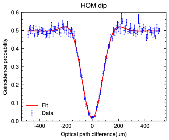
Figure S1: Hong-Ou-Mandel interference dip.

The HOMI visibility is closely related to the tomographic fidelity of the two-photon state. To check this, we first measure the HOMI dip, by setting $\theta=\pi/4$, which prepares the initial state as $\ket{\psi_{\text{in}}}=\ket{V}_{a}\ket{H}_{b}$. After post-selecting the case where both photons exit in path $a$, the prepared state is $\ket{\psi_{\alpha}}=\ket{1_{H},1_{V}}$. To observe interference in the polarization degree of freedom, we configure the evolution module as an identity operation by setting the QWP-HWP-QWP (QHQ) wave-plate group angles to Q($0^{\circ}$), H($0^{\circ}$), and Q($0^{\circ}$). The measurement module is set to Q($0^{\circ}$) and H($22.5^{\circ}$) to induce HOM interference in the polarization mode.

The observed HOM dip, shown in Fig. S1, is fitted using a model combining a Gaussian and a sinc function.

$$p_{\text{coin}}(x)=a-be^{-\frac{\sigma^{2}(x-x_{0})^{2}}{2}}\operatorname{sinc}(k(x-x_{0})),$$ (S55)

where $a$, $b$, $\sigma$, $x_{0}$, and $k$ are fitting parameters. The fit yields an interference visibility of $96.8\%$.

By varying $\theta$ from $0$ to $\pi/4$, we can prepare states in the form of $\ket{\psi_{\alpha}}=\cos\alpha\ket{2_{H},0}+\sin\alpha\ket{1_{H},1_{V}}$ with $0\leq\alpha\leq\pi/2$ as described in main text. Each state corresponds to a point $(x,y,z)$ in the traceless tangent space, as shown in Fig. 1(c). According to Eq. (S30), we have:

$$\rho_{\alpha}=\ket{\psi_{\alpha}}\!\!\bra{\psi_{\alpha}},$$ (S56)

$$(x,y,z)=\big{(}\tr(\rho H_{1}),\tr(\rho H_{2}),\tr(\rho H_{3})\big{)}=\left(\frac{1+\cos 2\alpha}{2\sqrt{2}},\frac{\sin 2\alpha}{2},0\right),$$

describing an ellipse centered at $(1/2\sqrt{2},0,0)$, with a major axis of $1/2$ and a minor axis of $1/2\sqrt{2}$. The tangent traceless invariant $I_{t^{\prime}}$ of $\rho_{\alpha}$ corresponding to the squared distance from the origin.

$\theta$	$\alpha$	$\ket{\psi_{\alpha}}$	$I_{t}$	$I_{p}$	$I_{t^{\prime}}$	$I_{o}$
$0^{\circ}$	$0^{\circ}$	$\ket{2_{H},0_{V}}$	0.833	0.167	0.5	4
$7.5^{\circ}$	$10.7^{\circ}$	$0.983\ket{2_{H},0_{V}}+0.186\ket{1_{H},1_{V}}$	0.833	0.167	0.500	3.998
$11.25^{\circ}$	$16.3^{\circ}$	$0.960\ket{2_{H},0_{V}}+0.281\ket{1_{H},1_{V}}$	0.830	0.170	0.497	3.988
$15^{\circ}$	$22.2^{\circ}$	$0.926\ket{2_{H},0_{V}}+0.378\ket{1_{H},1_{V}}$	0.823	0.177	0.490	3.959
$22.5^{\circ}$	$35.3^{\circ}$	$0.816\ket{2_{H},0_{V}}+0.577\ket{1_{H},1_{V}}$	0.778	0.222	0.445	3.778
$30^{\circ}$	$50.8^{\circ}$	$0.632\ket{2_{H},0_{V}}+0.775\ket{1_{H},1_{V}}$	0.653	0.347	0.320	3.280
$33.75^{\circ}$	$59.6^{\circ}$	$0.505\ket{2_{H},0_{V}}+0.863\ket{1_{H},1_{V}}$	0.556	0.444	0.223	2.891
$37.5^{\circ}$	$69.2^{\circ}$	$0.354\ket{2_{H},0_{V}}+0.935\ket{1_{H},1_{V}}$	0.451	0.549	0.118	2.471
$45^{\circ}$	$90^{\circ}$	$\ket{1_{H},1_{V}}$	0.333	0.667	0	2

Table S1: Theoretically calculated parameters of the prepared two-photon states: waveplate angle $\theta$, angle $\alpha$, state $\ket{\psi_{\alpha}}$, the tangent invariant $I_{t}$, the perpendicular invariant $I_{p}$, the traceless tangent invariant $I_{t^{\prime}}$, and the observable invariant $I_{o}$. Theoretically, $I_{t}+I_{p}=\tr(\rho^{2})=1$ as shown in Ref. [17], and $I_{t^{\prime}}=I_{t}-1/3,I_{o}=4I_{t^{\prime}}+2$ as derived in Theorem 2. These states correspond to the red points shown in Fig. 1(c)

The experimentally prepared states and their theoretical parameters are summarized in Table S1, corresponding to the red points in Fig. 1(c).

G.3 C. Compensation of Phase and Polarization Effects in NPBS-Based State Preparation

In our state preparation protocol, the NPBS introduces phase shifts in the transmission path and polarization distortions in the reflection path, both of which compromise the fidelity of the prepared quantum states. To mitigate these effects, we implemented tailored compensation strategies using wave plates for each path, as shown in Fig. 2(a) by the two QHQ wave-plate groups outlined within the dashed boxes.

For the transmission path: the NPBS in the transmission path induces a relative phase shift $\varphi$ between the $H$ and $V$ polarization components. For an input state $\frac{1}{\sqrt{2}}(\ket{H}+\ket{V})$, the transmitted state becomes $\frac{1}{\sqrt{2}}(\ket{H}+e^{i\varphi}\ket{V})$. After passing through a half-wave plate (HWP) oriented at 22.5^∘, the resulting state is $e^{i\varphi/2}\left(\cos\frac{\varphi}{2}\ket{H}-i\sin\frac{\varphi}{2}\ket{V}\right)$. Experimental measurements revealed that the $V$-component intensity post-interference was approximately 5% of the total intensity, corresponding to a phase shift of $\varphi=25^{\circ}$.

To correct this phase shift, we inserted QHQ wave-plate group before the NPBS, consisting of a quarter-wave plate at 45^∘, a half-wave plate at angle $\beta$, and another 45^∘ QWP. This wave-plate configuration has an effective Jones matrix given by:

$$\begin{pmatrix}e^{i2\beta}&0\\ 0&-e^{-i2\beta}\end{pmatrix}.$$ (S57)

By optimizing the angle $\beta$, we tuned the relative phase to counteract $\varphi$, reducing the $V$-component intensity to below 0.1% of the total intensity, thereby achieving robust phase compensation.

For the reflection path: the NPBS is intended to reflect $H$-polarized light exclusively. However, an unintended $V$-component emerges, with an initial intensity of 1.5% for an input state $\ket{H}$. To suppress this polarization impurity, we employed a QHQ wave-plate group positioned before the NPBS. Through iterative optimization of the wave plate angles, we refined this sequence to maintain the $H$-polarization, reducing the $V$-component intensity to below 0.1%.

The wave plate sequences implemented effectively minimize phase and polarization errors induced by the NPBS. For a more detailed analysis, quantum process tomography could be employed to fully characterize the NPBS-induced evolutions.

Appendix H VIII. Sampled Evolution unitary

Theoretically the state evolution induced by any LON preserve the invariant value. To experimentally verify this property, we implement various unitary evolutions. In this section, we first discuss the uniform sampling of $\mathrm{U}(2)$ [22] and subsequently describe the realization of the sampled $\mathrm{U}(2)$ scattering matrix using a QHQ waveplate configuration [46].

We parameterize $\mathrm{U}(2)$ as follows:

$$\phi=\arcsin\sqrt{\xi},$$ (S58)

$$U(\alpha,\phi,\psi,\chi)=e^{i\alpha}\begin{pmatrix}e^{i\psi}\cos\phi&e^{i\chi}\sin\phi\\ -e^{-i\chi}\sin\phi&e^{-i\psi}\cos\phi\end{pmatrix},$$

where $\alpha,\psi,\chi\in[0,2\pi]$ and $\xi\in[0,1]$ are uniformly sampled. The resulting unitary matrix $U(\alpha,\phi,\psi,\chi)$ is uniformly distributed over $\mathrm{U}(2)$ [22].

We set $\psi,\chi=\pi/2$ or $3\pi/2$, $\xi=1/3$ or $2/3$, and ignore the global phase $\alpha$, sampling eight matrices $\in\mathrm{U}(2)$. These unitary matrices are then realized experimentally using the QHQ wave-plate group [46]. The matrices parameters $\psi,\chi,\xi$ and corresponding QHQ wave-plate angle $Q(\theta_{1}),H(\theta_{2}),Q(\theta_{3})$ are listed in Table S2.

Number	$\psi$	$\chi$	$\xi$	$\theta_{1}$	$\theta_{2}$	$\theta_{3}$
$U_{1}$	$\pi/2$	$\pi/2$	$1/3$	24.1∘	17.6∘	101.2∘
$U_{2}$	$\pi/2$	$\pi/2$	$2/3$	149.5∘	27.4∘	175.2∘
$U_{3}$	$\pi/2$	$3\pi/2$	$1/3$	78.8∘	162.4∘	155.9∘
$U_{4}$	$\pi/2$	$3\pi/2$	$2/3$	4.8∘	152.6∘	30.5∘
$U_{5}$	$3\pi/2$	$\pi/2$	$1/3$	27.4∘	72.4∘	27.4∘
$U_{6}$	$3\pi/2$	$\pi/2$	$2/3$	81.9∘	62.6∘	133.3∘
$U_{7}$	$3\pi/2$	$3\pi/2$	$1/3$	152.6∘	107.6∘	152.6∘
$U_{8}$	$3\pi/2$	$3\pi/2$	$2/3$	98.1∘	117.4∘	46.7∘

Table S2: The sampled unitaries parameters $\psi,\chi,\xi$ and corresponding QHQ wave-plate angle $Q(\theta_{1}),H(\theta_{2}),Q(\theta_{3})$.

Appendix I IX. Multiphoton State Tomography

In this section, we detail the tomography procedure for a two-photon, two-mode polarization-encoded quantum state. The reconstruction of such a state requires a set of independent positive operator-valued measures (POVMs) to fully characterize the density matrix.

The measurement module, illustrated in Fig. 2(c) of the main text, consists of a polarization evolution and detection module. First, the multiphoton state is evolved QWP-HWP (QH) wave-plate group. The evolved state is then projected onto the photon-number basis using a beam displacer (BD), which spatially separates the horizontal ($H$) and vertical ($V$) polarization components. This results in three projection bases: $\ket{0_{H},2_{V}}$, $\ket{1_{H},1_{V}}$, and $\ket{2_{H},0_{V}}$.

Following this projection, two fiber beam splitter (BS) and four avalanche photodiodes (APDs, Excelitas Technologies, efficiency 55%, labeled 1–4 as in Fig. 2(c)) implement two pseudo photon-number-resolving detectors (PPNRD). Coincidence detection events are assigned as follows: $\{1,2\}$ for $\ket{2_{H},0_{V}}$, $\{1,3\}$, $\{1,4\}$, $\{2,3\}$, and $\{2,4\}$ for $\ket{1_{H},1_{V}}$, and $\{3,4\}$ for $\ket{0_{H},2_{V}}$.

To ensure a complete quantum state reconstruction, the measurement process requires a sufficient number of independent POVMs. Specifically, for each QH angle configuration, the corresponding POVM $\hat{E_{i}}$ take the form:

$$\hat{E_{1}}=V_{\text{QH}}^{\dagger}\hat{P}_{2_{H},0_{V}}V_{\text{QH}},\quad\hat{E_{2}}=V_{\text{QH}}^{\dagger}\hat{P}_{1_{H},1_{V}}V_{\text{QH}},\quad\hat{E_{3}}=V_{\text{QH}}^{\dagger}\hat{P}_{0_{H},2_{V}}V_{\text{QH}},$$ (S59)

where $V_{\text{QH}}$ represents the multiphoton unitary evolution induced by the QH waveplate group at the given angles, and $\hat{P}_{n_{H},m_{V}}=\ket{n_{H},m_{V}}\bra{n_{H},m_{V}}$ are the Fock state projectors for $\hat{P}_{2_{H},0_{V}}$, $\hat{P}_{1_{H},1_{V}}$, and $\hat{P}_{0_{H},2_{V}}$.

By varying QH angle configuration, we can construct more independent POVMs. It has been established that reconstructing an $N$-photon, $M$-mode quantum state using photon-counting detection combined with an $M$-mode LON requires at least [35]:

$$R_{N,M}=\binom{N+M}{N}-\binom{N+M-2}{M}$$ (S60)

distinct measurement configurations. For the case of two photons in two modes ($N=2,M=2$), this lower bound is five independent measurement settings.

We adopt six QH wave-plate settings chosen based on the configurations used in Ref. [39]. Specifically, the QWP and HWP angles are set to $(0^{\circ},0^{\circ})$, $(0^{\circ},11.25^{\circ})$, $(0^{\circ},22.5^{\circ})$, $(22.5^{\circ},0^{\circ})$, $(22.5^{\circ},22.5^{\circ})$, and $(45^{\circ},22.5^{\circ})$.

To verify the independence of the POVMs, we vectorize each $E_{i}$ (the matrix representation of $\hat{E}_{i}$ in the Fock state basis) and arrange them as row vectors. Constructing a matrix $\mathcal{M}$ whose rows are these vectorized $E_{i}$, we determine its rank to assess the number of linearly independent POVMs. The calculation confirms that nine independent POVMs are obtained. The use of an overcomplete measurement set $\{\hat{E_{i}}\}$ enhances fidelity and mitigates systematic errors, ensuring a more robust state reconstruction.

The density matrix $\rho$ finally obtained by solving a least-squares optimization problem that minimizes the objective function $f(\rho)$:

$$f(\rho)=\sum_{i}\left[\tr(\rho\,{E}_{i})-p_{i}\right]^{2},$$ (S61)

where $p_{i}$ represents the experimentally measured probability corresponding to the POVM ${E}_{i}$.