Multivariate Long-term Time Series Forecasting
with Fourier Neural Filter

Abstract

Multivariate long-term time series forecasting has been suffering from the challenge of capturing both temporal dependencies within variables and spatial correlations across variables simultaneously qiu2024tfb . Current approaches predominantly repurpose backbones from natural language processing or computer vision (e.g., Transformers), which fail to adequately address the unique properties of time series (e.g., periodicity) wang2025timemixer++ . The research community lacks a dedicated backbone with temporal-specific inductive biases, instead relying on domain-agnostic backbones supplemented with auxiliary techniques (e.g., signal decomposition). We introduce Fourier Neural Filter (FNF) as the backbone and Dual Branch Design (DBD) as the architecture to provide excellent learning capabilities and optimal learning pathways for spatio-temporal modeling, respectively. Our theoretical analysis proves that FNF unifies local time-domain and global frequency-domain information processing within a single backbone that extends naturally to spatial modeling, while information bottleneck theory demonstrates that DBD provides superior gradient flow and representation capacity compared to existing unified or sequential architectures. Our empirical evaluation across 11 public benchmark datasets spanning five domains (energy, meteorology, transportation, environment, and nature) confirms state-of-the-art performance with consistent hyperparameter settings. Notably, our approach achieves these results without any auxiliary techniques, suggesting that properly designed neural architectures can capture the inherent properties of time series, potentially transforming time series modeling in scientific and industrial applications.

1 Introduction

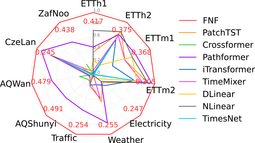
Figure 1: Radar chart of forecasting performance across 11 benchmark datasets spanning five domains. The chart displays average MAE across different forecast horizons of 96, 192, 336, 720. Our proposed FNF (highlighted) consistently outperforms eight strong baseline models on diverse domains of energy, weather, transportation, environment, and nature with consistent hyperparameter settings.

Time series forecasting, which predicts future values based on historical observations, has attracted substantial academic attention and found widespread application across diverse domains, including energy zhang2025machine and meteorology pathak2022fourcastnet ; bi2023accurate . Recent research has increasingly focused on multivariate long-term forecasting zhou2021informer , which presents several significant challenges. Extended forecast horizons inevitably increase uncertainty and degrade prediction accuracy, while complex temporal dependencies within variables and spatial correlations across variables further complicate modeling, particularly with high-dimensional variables. Consequently, developing neural architectures capable of simultaneously capturing heterogeneous temporal and spatial patterns has become critical for advancing time series forecasting.

For within-variable temporal modeling, the research community has developed several elaborate approaches. These include: (i) decomposing time series into trend, seasonal, and residual terms  taylor2018forecasting ; oreshkin2019n ; (ii) deconstructing time series into frequency components for multi-resolution modeling dai2024periodicity ; and (iii) segmenting sequences into patches of uniform nie2022time ; lee2023learning or varying sizes zhang2024multi ; yu2024prformer to capture both short-term fluctuations and long-term dependencies through multi-scale modeling. More sophisticated techniques integrate multi-resolution and multi-scale modeling simultaneously wang2025timemixer++ , establishing comprehensive frameworks for time series representation learning.

Despite these advances, existing approaches primarily rely on architectures borrowed from natural language processing or computer vision, such as Transformers vaswani2017attention , CNNs luo2024moderntcn ; wu2022timesnet , and MLPs zeng2023transformers . These domain-agnostic architectures cannot fully address the inherent properties of time series without auxiliary techniques (e.g., signal decomposition). To address this fundamental limitation, we propose the Fourier Neural Filter (FNF), a novel nonlinear integral kernel operator that integrates temporal-specific inductive biases directly into the backbone design. Mathematically, FNF extends the standard Fourier Neural Operator (FNO) li2020fourier by introducing an input-dependent kernel function that adaptively modulate information flow based on input properties. This design enables selective activation of local time-domain information and global frequency-domain information through Hadamard product operations, making it particularly effective for capturing the unique properties of time series. FNF offers several key advantages: (i) it naturally extends to spatial modeling guibas2021adaptive ; (ii) it achieves $O(N\log N)$ computational complexity compared to the $O(N^{2})$ complexity of Transformers; and (iii) it internally incorporates linear expansion operations, eliminating the need for dedicated feed-forward networks and reducing parameter count while maintaining performance.

For cross-variable spatial modeling, the researchers have developed diverse techniques: (i) independent variable modeling nie2022time ; dai2024periodicity , which maintains stability but ignores inter-variable interactions; (ii) unified variable modeling zhang2023crossformer , which comprehensively captures relationships but exhibits sensitivity to irrelevant variable disturbances; and (iii) hierarchical variable modeling chen2024similarity , which provides a compromise approach but constrains flexibility by confining relationship patterns within predetermined cluster boundaries. These techniques highlight the fundamental trade-offs in spatial modeling and emphasize the need for adaptive systems that optimize across these competing priorities.

To address above challenges, we propose the Dual Branch Design (DBD). From an information bottleneck perspective tishby2015deep , this parallel dual-branch architecture optimizes information extraction and compression in multivariate time series by maintaining separate processing pathways for temporal and spatial patterns. Unlike unified techniques that suffer from the curse of dimensionality or sequential techniques zhang2023crossformer ; chen2024pathformer that experience cascading information loss due to unequal information processing, DBD ensures that each branch independently achieves optimal trade-offs between information extraction and compression while providing shorter and more direct gradient flow.

To validate our approach, we conducted comprehensive experiments across 11 datasets spanning five domains (energy, meteorology, transportation, environment, and nature). Our extensive evaluation demonstrates that our approach achieves state-of-the-art results, as shown in Fig.˜1.

2 Related Work

Distribution Shift

The statistical properties of time series, such as mean and variance, tend to change over time, creating challenges for forecasting models passalis2019deep ; dai2024ddn ; liu2025timebridge . Researchers have developed various solutions to address this issue. RevIN kim2021reversible applies instance normalization on input sequences and performs de-normalization on output sequences. Dish-TS fan2023dish extracts distribution coefficients for both intra- and inter-variable dimensions to mitigate distribution shift. SAN liu2023adaptive addresses non-stationarity at the local temporal slice level using a lightweight network to model evolving statistical properties. FAN ye2024frequency handles dynamic trends and seasonal patterns by employing Fourier transform to identify key frequency components across instances. Notably, Li et al. li2023revisiting demonstrated that after using instance normalization, excellent results can be easily obtained with just a simple linear layer. Our approach employs basic instance normalization while introducing a backbone that inherently processes time-domain and frequency-domain information simultaneously.

Patch Embedding

Time series patching has evolved from simple segmentation to sophisticated strategies that balance local and global information extraction nie2022time ; lee2023learning . These techniques include overlapping nie2022time ; luo2024moderntcn or non-overlapping zhang2023crossformer patching, variable length patching yu2024prformer ; zhang2024multi , and hierarchical patching huang2024hdmixer . Recent research has explored adaptive patching strategies based on input properties of time series chen2024pathformer . While these approaches enhance representation capabilities, they primarily function as preprocessing steps for conventional architectures. Our work adopts basic overlapping patching for fair comparison while introducing the FNF backbone specifically designed to unify local time-domain and global frequency-domain processing for time series.

Non-Autoregressive

To alleviate the error accumulation problem in autoregressive decoding, non-autoregressive approaches wu2021autoformer ; zhou2021informer ; wu2022timesnet ; liu2023itransformer have become the standard paradigm for long-term time series forecasting. This technique simultaneously generates all future values through a linear layer, rather than recursively using previous predictions as inputs. While patch-based autoregressive models excel in large-scale time series foundation models das2024decoder ; shi2024time , non-autoregressive approaches perform better in typical forecasting scenarios. Recent research has identified that non-autoregressive approaches implicitly assume conditional independence between future values, ignoring the temporal autocorrelation inherent in time series wang2024fredf . Our proposed FNF and DBD enhance representation learning quality within this established architecture, improving forecasting accuracy despite the theoretical limitations of the non-autoregressive paradigm.

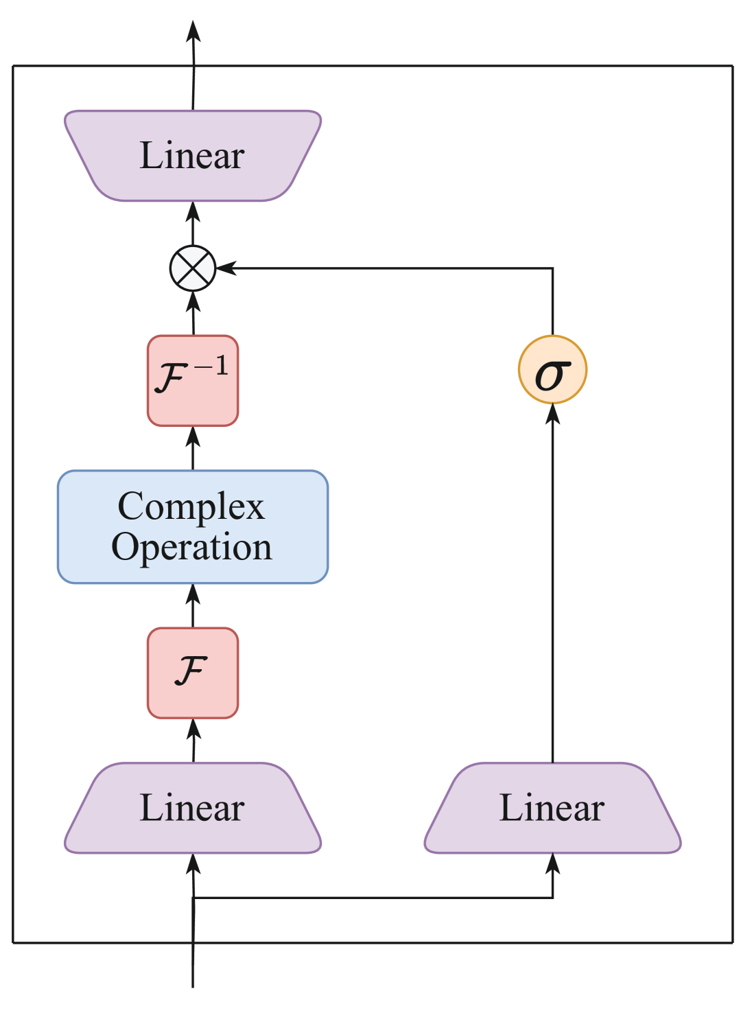
Figure 2: The FNF backbone. Our dual-branch design processes input embeddings through parallel expanded linear layers gu2024mamba . The right branch captures time-domain patterns via GELU activation hendrycks2016gaussian , while the left branch extracts frequency-domain features through Fourier transform, complex operations guibas2021adaptive (two complex linear layers with Softshrink function donoho2002noising ), and inverse Fourier transform. The branches are combined via Hadamard product ($\odot$), enabling simultaneous modeling of local temporal and global spectral information.

3 Methodology

This section establishes the theoretical foundations of our proposed Fourier Neural Filter (FNF) backbone and the Dual Branch Design (DBD) architecture.

3.1 The Fourier Neural Filter (FNF) Backbone

While FNO li2020fourier has demonstrated remarkable effectiveness in modeling complex dynamic systems and solving partial differential equations through fixed integration kernels, our proposed FNF (Fig.˜2) introduces a critical advancement—an input-dependent integral kernel that significantly enhances flexibility and generalization capacity. We analyze the theoretical underpinnings of FNF by examining integral kernel functions, global convolution operations, selective activation mechanisms, and their connections to Transformer architectures.

3.1.1 Integral Kernel

Definition 1

FNO li2020fourier is defined through an integral kernel operator:

$$(Kv)(x)=\int_{D}\kappa(x,y)v(y)\,dy,$$ (1)

where $\kappa:D\times D\rightarrow\mathbb{R}$ is the kernel function and $v:D\rightarrow\mathbb{R}$ is the input function. Through the Fourier transform, FNO can be formulated in the frequency domain as:

$$(Kv)(x)=\mathcal{F}^{-1}(R_{\phi}\cdot\mathcal{F}(v))(x),$$ (2)

where $R_{\phi}=\mathcal{F}(\kappa)$ denotes the parameterized frequency-domain kernel.

Definition 2

FNF extends this concept through a generalized integral kernel operator:

$$(Kv)(x)=\int_{D}\kappa(x,y;v)v(y)\,dy,$$ (3)

where the kernel function $\kappa(x,y;v)$ is input-dependent. In implementation, FNF takes the form:

$$(Kv)(x)=T(G(v)(x)\odot\mathcal{F}^{-1}(R_{\phi}\cdot\mathcal{F}(H(v)))(x)),$$ (4)

where $T(v)$, $G(v)$, and $H(v)$ represent linear transformations, with $G$ activated by GELU hendrycks2016gaussian , and $\odot$ denoting the Hadamard product operation.

Remark 1

The fundamental distinction between FNO and FNF lies in their kernel functions: FNO employs a fixed kernel $\kappa(x,y)$, whereas FNF utilizes an input-dependent kernel $\kappa(x,y;v)$, enabling adaptive information flow modulation based on input properties.

3.1.2 Global Convolution

Definition 3

When the kernel function $\kappa(x,y)=\kappa(x-y)$ exhibits translation invariance, the integral kernel operator in FNO reduces to a global convolution li2020fourier :

$$(Kv)(x)=\int_{D}\kappa(x-y)v(y)\,dy=(\kappa*v)(x).$$ (5)

Definition 4

Similarly, when the kernel function $\kappa(x,y;v)=\kappa(x-y;v)$ maintains translation invariance, the integral kernel operator in FNF becomes a gated global convolution:

$$(Kv)(x)=\int_{D}\tilde{\kappa}(x-y;v)v(y)\,dy=(\tilde{\kappa}(\cdot;v)*v)(x).$$ (6)

Remark 2

Translation invariance provides a computational advantage for both FNO and FNF, enabling efficient implementation through Fourier domain operations. However, the gated global convolution of FNF introduces enhanced expressivity through its input-dependent kernel $\tilde{\kappa}(\cdot;v)$, which dynamically adapts its filtering behavior while preserving the computational efficiency of convolution operations.

3.1.3 Selective Activation

Definition 5

The selective activation mechanism in FNF operates through Hadamard product between local information $G(v)(x)$ and global information $P(v)(x)$:

$$(G(v)\odot P(v))_{i}=|G(v)_{i}|\cdot|P(v)_{i}|\cdot e^{i(\theta_{G(v)_{i}}+\theta_{P(v)_{i}})},$$ (7)

where $|G(v)_{i}|$ and $|P(v)i|$ represent magnitudes and $\theta{G(v)i}$ and $\theta{P(v)_{i}}$ represent phases.

Remark 3

This formulation reveals how selective activation simultaneously modulates both amplitude (through multiplication $|G(v)_{i}|\cdot|P(v)_{i}|$) and phase (through addition $\theta_{G(v)_{i}}+\theta_{P(v)_{i}}$). This joint modulation in complex space enables precise control over both intensity and orientation of features, providing substantially enhanced representational capacity compared to conventional approaches.

Remark 4

In FNF, selective activation facilitates adaptive fusion of local and global information. The local information $G(v)$ functions as a gating mechanism that regulates global information flow from $P(v)$ at each position. This creates three distinct operational modes: suppression when $|G(v)_{i}|\approx 0$, preservation when $|G(v)_{i}|\approx 1$, and amplification when $|G(v)_{i}|>1$, allowing FNF to dynamically balance local details with global context by focusing computational resources on the most informative regions.

3.1.4 Complex Operation

Definition 7

Complex linear transformation guibas2021adaptive operates on complex-valued input $z=z_{r}+iz_{i}$ with complex weights $W=W_{r}+iW_{i}$ and biases $b=b_{r}+ib_{i}$:

$$L(z)=(W_{r}z_{r}-W_{i}z_{i}+b_{r})+i(W_{r}z_{i}+W_{i}z_{r}+b_{i}).$$ (8)

Remark 5

Complex activation functions typically apply standard nonlinear activations like ReLU nair2010rectified separately to real and imaginary components: $\sigma_{\mathbb{C}}(z)=\sigma(z_{r})+i\sigma(z_{i})$. In our implementation, we employ GELU hendrycks2016gaussian as the complex activation function.

Definition 8

The Softshrink operation donoho2002noising for frequency domain denoising is defined as:

$$S_{\lambda}(z)=\begin{cases}(|z|-\lambda)\frac{z}{|z|},&\text{if }|z|>\lambda\\ 0,&\text{if }|z|\leq\lambda,\end{cases}$$ (9)

where $\lambda$ is the threshold parameter.

Remark 6

The Softshrink operation preserves phase while adaptively sparsifying the frequency spectrum by eliminating components below threshold $\lambda$, effectively filtering noise while maintaining significant frequency information.

3.1.5 Connection to Transformers

Functionality

FNF represents a unified backbone that implements core Transformer functions through alternative computational mechanisms. The gated global convolution in FNF performs comprehensive information exchange across all positions, analogous to token mixing in self-attention. Furthermore, the linear transformations ($T(v)$, $G(v)$, and $H(v)$) in FNF can be expanded to replicate the functionality of feed-forward networks, establishing functional equivalence between architectures while maintaining distinct computational pathways.

Complexity

FNF achieves token mixing with $O(N\log N)$ computational complexity through Fourier transform operations, compared to the $O(N^{2})$ complexity of standard Transformers for sequence length $N$. Moreover, FNF typically requires fewer parameters while maintaining comparable expressivity, making it particularly efficient for modeling long-range dependencies in high-dimensional temporal sequences.

3.2 The Dual Branch Design (DBD) Architecture

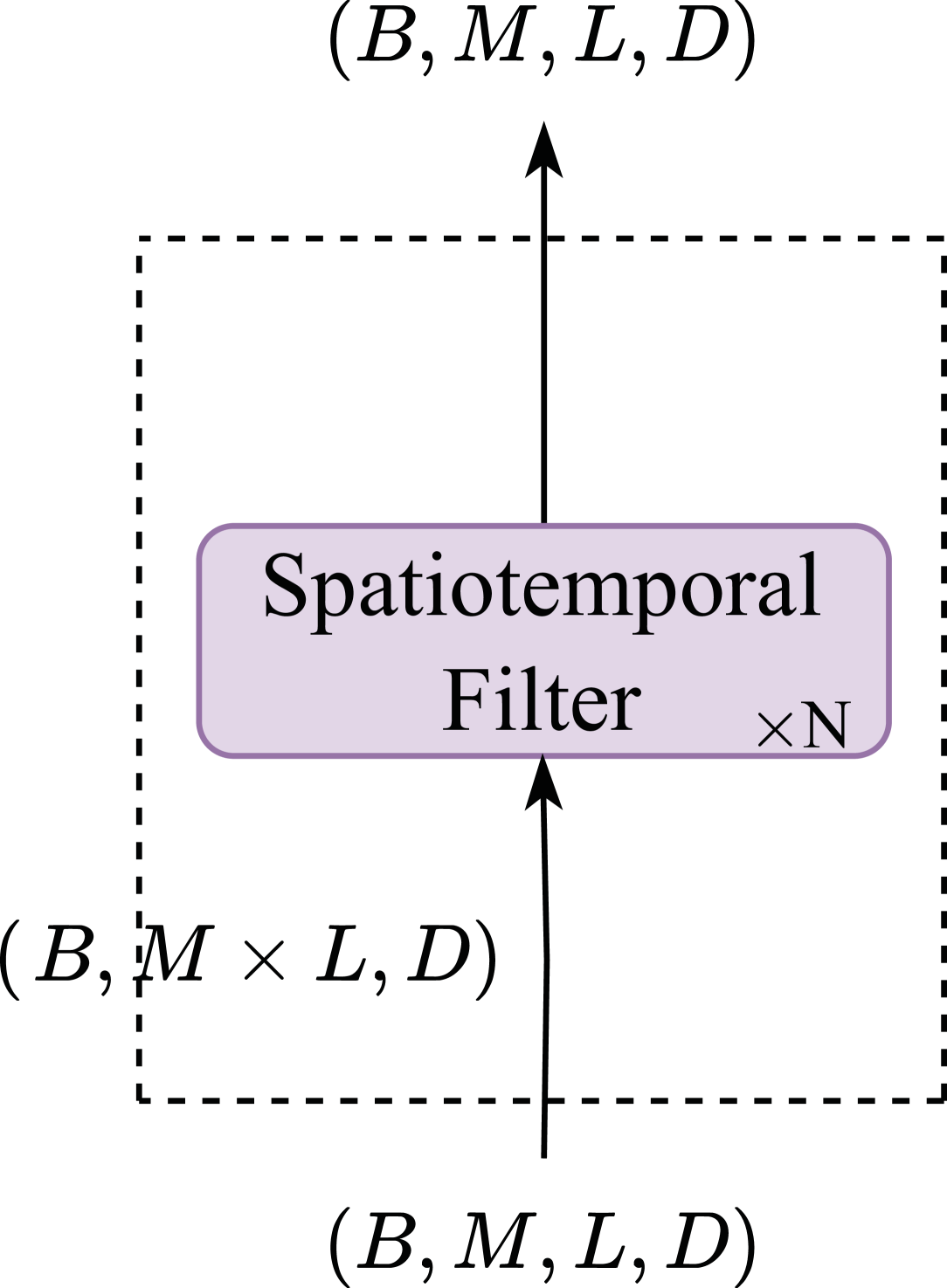
(a) Unified

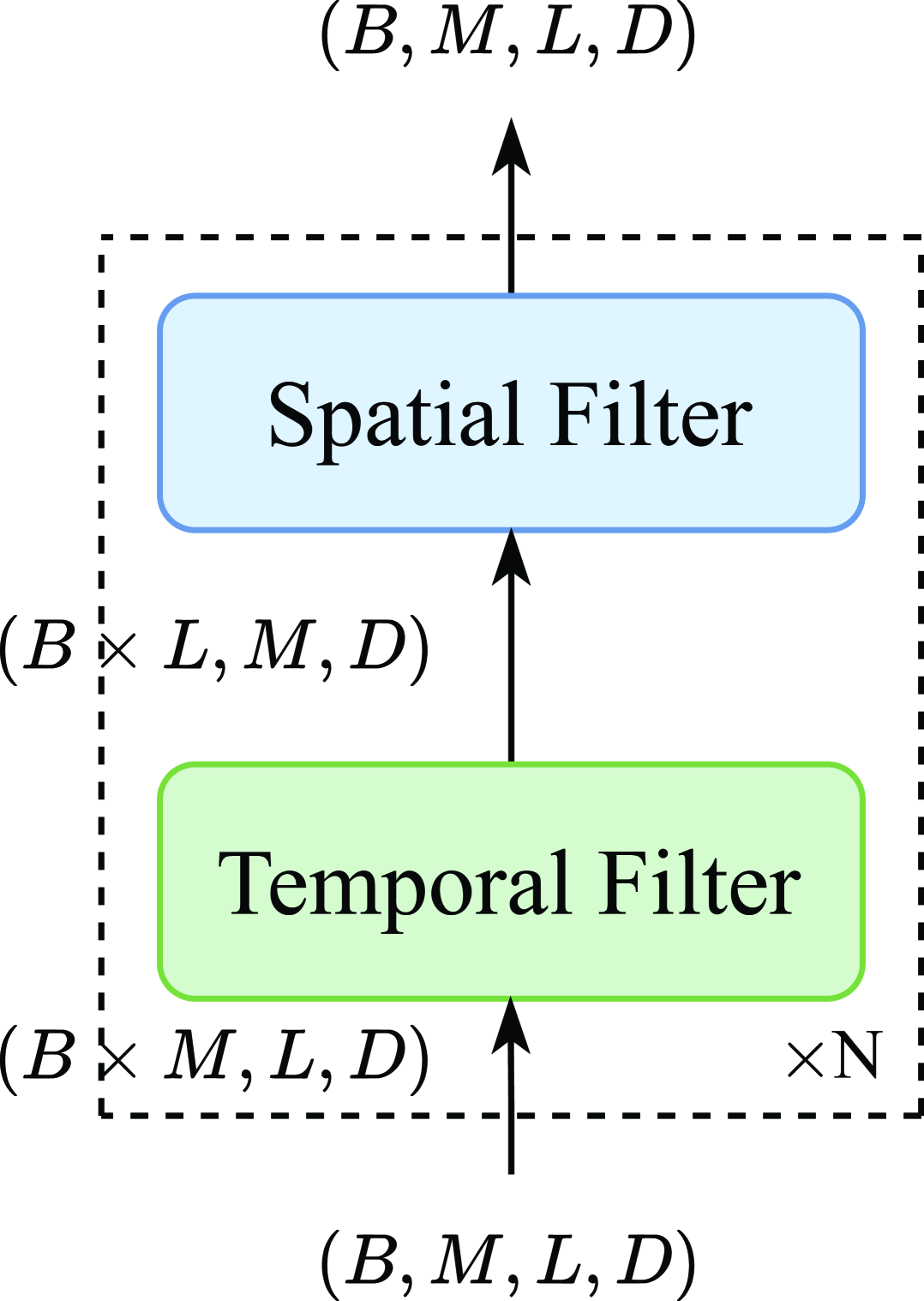
(b) Sequential

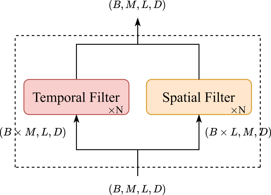
(c) Parallel

Figure 3: The Dual Branch Design (DBD) architecture. Each approach processes multivariate time series in shape $(B,M,L,D)$ differently: (a) Unified: single backbone simultaneously models temporal and spatial patterns; (b) Sequential: cascades temporal filter followed by spatial filter; (c) Parallel: applies independent temporal and spatial filters in separate branches. Our DBD implements the parallel design to effectively perform temporal and spatial modeling.

Through the lens of information bottleneck theory tishby2015deep , spatiotemporal modeling architectures can be categorized into three paradigms (Fig.˜3): unified (which suffers from the curse of dimensionality) alemi2016deep , sequential (which creates information bottlenecks) zhang2023crossformer ; chen2024pathformer , and parallel (which preserves information through independent branches). Our DBD architecture adopts the parallel approach to maximize gradient flow and representation capacity.

Unified

The unified paradigm captures temporal and spatial, and spatiotemporal patterns through a single operation, formulated as:

$$X\rightarrow T\rightarrow Y,$$ (10)

where $T$ represents a high-dimensional intermediate representation. As $T$ must simultaneously encode both temporal and spatial information, finding the optimal balance between compression and informativeness becomes computationally intractable. This approach requires substantially more parameters to achieve comparable expressiveness, increasing overfitting risk and reducing generalization performance.

Sequential

The sequential paradigm implements a cascaded architecture where temporal processing precedes spatial processing:

$$X\rightarrow T_{1}\rightarrow T_{2}\rightarrow Y,$$ (11)

where $T_{1}$ and $T_{2}$ denote temporal and spatial representations, respectively. According to the information processing inequality, this architecture inherently suffers from information loss:

$$I(X;Y)\geq I\left(T_{1};Y\right)\geq I\left(T_{2};Y\right).$$ (12)

Each processing stage acts as an information bottleneck, potentially discarding critical temporal patterns before they reach the spatial processing stage. Additionally, gradients must propagate through multiple transformation layers, often leading to vanishing gradient problems.

Parallel

The parallel paradigm maintains independent information processing branches with direct access to the original input wang2018non :

$$X\rightarrow\left\{\begin{array}[]{l}T_{1}\\ T_{2}\end{array}\rightarrow T\rightarrow Y\right..$$ (13)

This approach ensures each branch independently achieves optimal information compression, with each optimizing its own objective function:

$$\min_{T_{1}}\left[I\left(T_{1};X\right)-\beta_{1}I\left(T_{1};Y\right)\right]$$ (14)

$$\min_{T_{2}}\left[I\left(T_{2};X\right)-\beta_{2}I\left(T_{2};Y\right)\right],$$

where $\beta_{1}$ and $\beta_{2}$ control the trade-off between compression and performance for each branch. This allows temporal and spatial processors to specialize without constraints imposed by the other branch.

Gradient Flow

The parallel architecture offers significant advantages in terms of gradient flow. With independent branches, the gradient paths remain short and direct:

$$\frac{\partial L}{\partial\theta_{1}} =\frac{\partial L}{\partial g}\cdot\frac{\partial g}{\partial f_{1}}\cdot\frac{\partial f_{1}}{\partial\theta_{1}}$$ (15)

$$\frac{\partial L}{\partial\theta_{2}} =\frac{\partial L}{\partial g}\cdot\frac{\partial g}{\partial f_{2}}\cdot\frac{\partial f_{2}}{\partial\theta_{2}}.$$

These shorter gradient paths significantly reduce the risk of vanishing or exploding gradients that typically plague deeper sequential architectures. Additionally, the independent branches enable more efficient parallelization during both forward and backward passes, accelerating convergence without sacrificing model expressiveness.

Representation Capacity

The parallel architecture demonstrates superior representation capacity through its ability to retain and complement information. The theoretical upper bound on mutual information is given by:

$$I\left(T;Y\right)\leq I\left(T_{1},T_{2};Y\right).$$ (16)

Due to the complementary nature of temporal and spatial information, the joint representation typically satisfies:

$$I\left(T_{1},T_{2};Y\right)>\max\left\{I\left(T_{1};Y\right),I\left(T_{2};Y\right)\right\}.$$ (17)

This inequality holds because temporal and spatial features capture fundamentally orthogonal aspects of the input—temporal features extract dynamic patterns across time, while spatial features encode structural relationships within each time point. Their combination provides a more comprehensive view than either branch could achieve alone. Furthermore, the parallel approach enables adaptive information fusion through a learnable, input-dependent weights:

$$T=\alpha(X)\cdot T_{1}+(1-\alpha(X))\cdot T_{2}.$$ (18)

This dynamic weighting mechanism contextually assesses the relative importance of each information flow, effectively addressing varying requirements across different scenarios and input characteristics.

4 Model Implementation

Overview

We denote the lookback window as $X=\left(x_{1},\ldots,x_{T}\right)\in\mathbb{R}^{L\times M}$ with $L$ timesteps and $M$ variables, and the forecast horizon as $Y=\left(y_{1},\ldots,y_{L}\right)\in\mathbb{R}^{H\times M}$ with $H$ timesteps.

As illustrated in Fig.˜4, our pipeline integrates specialized components—normalization, embedding, dual-branch backbone, projection, and de-normalization—each addressing specific aspects of the forecasting challenge.

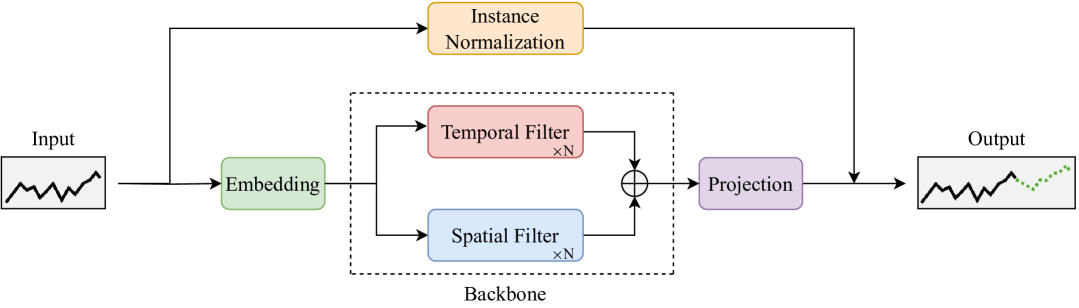
Figure 4: Schematic diagram of our proposed neural architecture. Where, normalization for mitigating distribution shift, embedding for obtaining informative input embeddings, backbone for addressing temporal dependencies and spatial correlations, and projection for generating predicted values.

Normalization

To address distribution shift inherent in the time series, we implement instance normalization kim2021reversible :

$$X=\frac{X-\mu}{\sigma+\epsilon},$$ (19)

where $\mu$ and $\sigma$ represent the mean and standard deviation vectors of the input sequence, with $\epsilon$ added for numerical stability.

Embedding

We transform the normalized sequences using patch embedding nie2022time to enhance feature representation:

$$X=\text{Patching}(X)+\text{PE},$$ (20)

where Patching segments time series into overlapping patches, and PE incorporates sine-cosine positional encoding to preserve temporal ordering.

Backbone

The core design leverages a parallel dual-branch architecture with adaptive gated mechanism:

$$X=\alpha\cdot\text{\acs{fnf}}_{1}(X)+(1-\alpha)\cdot\text{\acs{fnf}}_{2}(X),$$ (21)

where $\text{\acs{fnf}}_{1}$ extracts temporal dependencies while $\text{\acs{fnf}}_{2}$ captures spatial correlations across variables. The dynamic gating coefficient $\alpha=\sigma(W\cdot\text{\acs{fnf}}_{1}(X)+b)$ adaptively balances these complementary information streams, with $\sigma$ representing the sigmoid activation rumelhart1986learning , and $W$ and $b$ as learnable parameters.

Projection

The processed embeddings are transformed into predictions through a straightforward linear projection:

$$Y=\text{Linear}(\text{Flatten}(X)),$$ (22)

where flattening and linear transformation efficiently map the embedded features to the normalized output space.

De-normalization

Finally, we restore the predictions to their original scale:

$$Y=Y\cdot(\sigma+\epsilon)+\mu,$$ (23)

applying the inverse of the normalization process to obtain future values.

5 Experiments

Datasets

To thoroughly evaluate our model performance across diverse domains, we conduct experiments on 11 real-world datasets spanning 5 distinct domains, as detailed in Tab.˜1. These include energy (ETTh1, ETTh2, ETTm1, ETTm2, and Electricity) zhou2021informer , meteorology (Weather) wu2021autoformer , transportation (Traffic) wu2021autoformer , environment (AQShunyi and AQWan) zhang2017cautionary , and nature (ZafNoo and CzeLan) poyatos2020global .

Table 1: Dataset overview.

Domain	Dataset	Frequency	Length	Variable
Energy	ETTh1	1 hour	14,400	7
	ETTh2	1 hour	14,400	7
	ETTm1	15 min	57,600	7
	ETTm2	15 min	57,600	7
	Electricity	1 hour	26,304	321
Meteorology	Weather	10 min	52,696	21
Transportation	Traffic	1 hour	17,544	862
Environment	AQShunyi	1 hour	35,064	11
	AQWan	1 hour	35,064	11
Nature	ZafNoo	2 min	19,225	11
	CzeLan	30 min	19,954	11

Baselines

We benchmark our approach against recent state-of-the-art models across three architectural paradigms: (i) Transformer-based models: Pathformer chen2024pathformer , PatchTST nie2022time , Crossformer zhang2023crossformer , and iTransformer liu2023itransformer ; (ii) MLP-based models: TimeMixer wang2024timemixer , DLinear zeng2023transformers , and NLinear zeng2023transformers ; and (iii) CNN-based models: TimesNet wu2022timesnet .

Settings

We implement all experiments using PyTorch 2.5 in Python 3.10, with computations performed on an NVIDIA H100 GPU. In accordance with the Time Series Forecasting Benchmark (TFB) protocol qiu2024tfb , baseline results represent optimal performance obtained across various lookback windows (96, 336, and 512). All models are trained using L1 loss and optimized with the Adam optimizer. For our approach, we standardize on a lookback window of 512. We maintain consistent hyperparameters across experiments—patch size of 16, stride of 8, embedding dimension of 128, expansion ratio of 2, 3 backbone layers, batch size of 128, and learning rate of 0.0001—with the exception of larger datasets like Traffic, where we reduce the batch size to 24 to accommodate memory constraints. Following established evaluation practices, we assess performance using Mean Squared Error (MSE) and Mean Absolute Error (MAE) metrics.

Table 2: Multivariate long-term forecasting performance. Average MSE and MAE across forecast horizons (96, 192, 336, 720) on 11 datasets. Best results in bold, second-best underlined. FNF consistently outperforms baselines, particularly in MAE.

Models	FNF		PatchTST		Crossformer		Pathformer		iTransformer		TimeMixer		DLinear		NLinear		TimesNet
Metrics	MSE	MAE	MSE	MAE	MSE	MAE	MSE	MAE	MSE	MAE	MSE	MAE	MSE	MAE	MSE	MAE	MSE	MAE
ETTh1	0.403	0.417	0.410	0.428	0.452	0.466	0.417	0.426	0.438	0.448	0.427	0.441	0.419	0.432	0.410	0.421	0.458	0.455
ETTh2	0.327	0.375	0.346	0.389	0.860	0.670	0.359	0.394	0.370	0.403	0.349	0.396	0.492	0.478	0.342	0.389	0.393	0.416
ETTm1	0.347	0.368	0.348	0.380	0.464	0.457	0.357	0.374	0.361	0.389	0.355	0.380	0.354	0.376	0.358	0.376	0.430	0.427
ETTm2	0.249	0.305	0.255	0.312	0.589	0.534	0.252	0.308	0.268	0.327	0.256	0.318	0.259	0.324	0.253	0.312	0.294	0.331
Electricity	0.157	0.247	0.163	0.260	0.180	0.279	0.168	0.261	0.162	0.258	0.184	0.284	0.166	0.264	0.169	0.261	0.185	0.286
Weather	0.226	0.255	0.224	0.262	0.234	0.294	0.224	0.257	0.232	0.269	0.226	0.263	0.239	0.289	0.249	0.280	0.261	0.287
Traffic	0.402	0.254	0.404	0.282	0.523	0.283	0.416	0.263	0.397	0.280	0.409	0.279	0.433	0.295	0.433	0.290	0.626	0.328
AQShunyi	0.695	0.491	0.704	0.508	0.694	0.504	0.722	0.495	0.705	0.506	0.706	0.506	0.705	0.522	0.713	0.514	0.726	0.515
AQWan	0.788	0.479	0.811	0.499	0.786	0.489	0.817	0.482	0.809	0.495	0.809	0.494	0.817	0.511	0.825	0.504	0.813	0.500
CzeLan	0.215	0.245	0.226	0.289	0.955	0.576	0.226	0.252	0.217	0.272	0.218	0.267	0.284	0.342	0.228	0.269	0.224	0.285
ZafNoo	0.515	0.438	0.511	0.465	0.482	0.447	0.520	0.441	0.522	0.456	0.517	0.451	0.496	0.451	0.522	0.457	0.537	0.465

Results

Due to space constraints, we report the average MSE and MAE across all forecast horizons for each dataset, with complete experimental results provided in the Appendix. As shown in Tab.˜2, our approach achieves state-of-the-art performance across all 11 public benchmark datasets. Notably, we observe an interesting phenomenon: our model demonstrates more substantial improvements in MAE compared to MSE when measured against baseline models. This pattern suggests that our approach produces more accurate predictions at the majority of timesteps (yielding lower overall MAE), while potentially generating larger errors at a few unpredictable extreme points or outliers (which disproportionately impact MSE due to the squaring operation).

This characteristic is particularly advantageous for long-term time series forecasting for several reasons. First, maintaining smaller errors across most timesteps is crucial for accurately capturing long-term trends. Second, our frequency domain modeling approach effectively captures primary periodic patterns, significantly reducing overall prediction bias. Third, from a practical perspective, consistently accurate predictions across the majority of timesteps typically delivers greater operational value than precisely predicting isolated extreme events.

Table 3: Backbone ablation study. Performance comparison of Transformer, FNO, and FNF across forecast horizons on ETTh1 and ETTh2 datasets. Best results in bold, second-best underlined.

Models		Transformer(I)		FNO(I)		FNF(I)		FNF(P)
Metrics		MSE	MAE	MSE	MAE	MSE	MAE	MSE	MAE
ETTh1	96	0.376	0.396	0.362	0.387	0.360	0.385	0.355	0.388
	192	0.399	0.416	0.401	0.409	0.407	0.414	0.396	0.412
	336	0.418	0.432	0.433	0.433	0.440	0.434	0.425	0.425
	720	0.450	0.469	0.448	0.467	0.428	0.449	0.436	0.445
	Avg	0.410	0.428	0.411	0.424	0.408	0.420	0.403	0.417
ETTh2	96	0.277	0.339	0.274	0.329	0.270	0.327	0.266	0.326
	192	0.345	0.381	0.346	0.375	0.337	0.370	0.331	0.371
	336	0.368	0.404	0.341	0.390	0.328	0.376	0.336	0.388
	720	0.397	0.432	0.398	0.431	0.386	0.423	0.378	0.418
	Avg	0.346	0.389	0.339	0.381	0.330	0.374	0.327	0.375

Ablations

We conduct comprehensive ablation studies to validate the effectiveness of our proposed FNF and DBD approaches. In our notation, we use I (variable-independent), U (unified architecture), S (sequential architecture), and P (parallel architecture) to denote different architectural designs. Tab.˜3 presents performance comparisons across different backbone designs—Transformer(I), FNO(I), FNF(I), and FNF(P)—evaluated under identical settings on the ETTh1 and ETTh2 datasets. The results clearly demonstrate that FNF(I) substantially outperforms both FNO(I) and Transformer(I), confirming the effectiveness of our proposed frequency-based neural filtering approach. Furthermore, the superior performance of FNF(P) compared to FNF(I) validates the enhanced capability of our parallel architecture to capture complex spatial correlations within multivariate time series.

To further investigate the impact of different architectural designs, we evaluate FNF(I), FNF(U), FNF(S), and FNF(P) under identical configurations on the CzeLan and ZafNoo datasets. As shown in Tab.˜4, FNF(P) substantially outperforms all alternative architectures across both benchmarks, providing compelling evidence for the effectiveness of our parallel design. A particularly revealing finding is that both FNF(U) and FNF(S) underperform compared to the simpler variable-independent FNF(I) baseline. This indicates that suboptimal approaches to modeling spatial relationships can actually degrade performance rather than enhance it. This observation underscores the critical importance of our proposed parallel architecture, which effectively captures complex inter-variable relationships while preserving the integrity of intra-variable temporal patterns. These results collectively validate our architectural choices and demonstrate the superiority of the parallel approach for multivariate long-term time series forecasting tasks.

Table 4: Architecture ablation study. Comparison of variable-independent (I), unified (U), sequential (S), and parallel (P) architectures on CzeLan and ZafNoo datasets. Best results in bold, second-best underlined.

Models		FNF(I)		FNF(U)		FNF(S)		FNF(P)
Metrics		MSE	MAE	MSE	MAE	MSE	MAE	MSE	MAE
CzeLan	96	0.171	0.207	0.175	0.214	0.172	0.214	0.170	0.208
	192	0.200	0.230	0.204	0.235	0.206	0.239	0.200	0.231
	336	0.232	0.258	0.233	0.261	0.240	0.269	0.228	0.257
	720	0.273	0.291	0.271	0.293	0.272	0.295	0.262	0.286
	Avg	0.219	0.246	0.220	0.250	0.222	0.254	0.215	0.245
ZafNoo	96	0.440	0.393	0.447	0.396	0.448	0.396	0.437	0.389
	192	0.500	0.433	0.508	0.437	0.509	0.435	0.498	0.429
	336	0.540	0.457	0.547	0.459	0.547	0.458	0.539	0.453
	720	0.587	0.485	0.588	0.484	0.589	0.488	0.588	0.483
	Avg	0.516	0.442	0.522	0.444	0.523	0.444	0.515	0.438

Sensitivities

We also examine the effect of different lookback windows on model performance, evaluating our FNF model with lookback windows of 96, 336, 512, and 720, as presented in Tab.˜5. Our results generally demonstrate performance improvements with increased lookback windows, with the most substantial gains observed when extending from 96 to 336. This pattern reflects the enhanced ability of our model to capture long-term dependencies with access to longer contexts. However, we find that larger lookback windows do not universally guarantee improved performance. For instance, in the AQWan dataset, the results get worse when the lookback window increases from 512 to 720, suggesting that excessively longer contexts may introduce noise or dilute the relevance of more recent patterns. Additionally, larger lookback windows impose increased computational demands, creating an important practical trade-off between forecasting accuracy and computational efficiency. These findings highlight the importance of tailoring lookback window to specific dataset characteristics and application requirements, rather than defaulting to maximum available context.

Table 5: Lookback window sensitivity analysis. Model performance of FNF(P) with varying lookback windows (96, 336, 512, and 720) on AQShunyi and AQWan datasets. Best results in bold, second-best underlined.

Models		FNF(96)		FNF(336)		FNF(512)		FNF(720)
Metrics		MSE	MAE	MSE	MAE	MSE	MAE	MSE	MAE
AQShunyi	96	0.702	0.482	0.640	0.465	0.629	0.461	0.626	0.465
	192	0.757	0.506	0.691	0.485	0.685	0.484	0.679	0.484
	336	0.773	0.517	0.711	0.497	0.704	0.497	0.699	0.497
	720	0.806	0.534	0.767	0.522	0.764	0.522	0.749	0.516
	Avg	0.759	0.509	0.702	0.492	0.695	0.491	0.688	0.490
AQWan	96	0.799	0.473	0.730	0.455	0.711	0.446	0.728	0.456
	192	0.856	0.496	0.786	0.477	0.773	0.473	0.786	0.480
	336	0.879	0.506	0.798	0.486	0.799	0.486	0.801	0.488
	720	0.945	0.531	0.863	0.508	0.869	0.514	0.889	0.523
	Avg	0.869	0.501	0.794	0.481	0.788	0.479	0.801	0.486

6 Conclusion

Limitations

While our approach demonstrates state-of-the-art performance across multiple domains, several important limitations merit consideration. First, despite effectively capturing both temporal and spatial patterns in regular time series, our model may struggle with extremely irregular or event-driven sequences where underlying patterns are less predictable. Second, although our approach achieves theoretical computational efficiency of $O(N\log N)$ compared to Transformers of $O(N^{2})$, practical implementation still presents challenges for extremely long sequences or resource-constrained real-time applications. Third, our current evaluation focuses exclusively on multivariate long-term forecasting; the effectiveness for other critical time series tasks—including imputation, classification, and anomaly detection—remains unexplored and represents a key direction for future research.

Broader Impact

Our work offers significant potential benefits across domains requiring accurate long-term forecasting. In energy systems, enhanced forecasting can improve grid stability and facilitate greater renewable energy integration. In transportation networks, precise predictions enable more efficient resource allocation and infrastructure planning. In environmental monitoring, reliable forecasts support improved disaster preparedness and climate adaptation strategies. However, we must acknowledge several potential risks: forecasting systems may inadvertently perpetuate historical biases embedded in training data; advanced computational requirements could widen the technology gap between well-resourced organizations and those with limited capabilities; and there exists danger of excessive reliance on automated predictions in critical decision contexts without appropriate human oversight. We encourage the research community to address these concerns through dedicated efforts toward fairness, interpretability, and accessibility.

Appendix A Dataset Details

We provide a more detailed introduction for each dataset as shown in Tab.˜A1. More details can be found in the Tab.˜1.

Table A1: Dataset description.

Dataset	Description
ETTh1 [6]	Power transformer 1, comprising seven indicators such as oil temperature and useful load
ETTh2 [6]	Power transformer 2, comprising seven indicators such as oil temperature and useful load
ETTm1 [6]	Power transformer 1, comprising seven indicators such as oil temperature and useful load
ETTm2 [6]	Power transformer 2, comprising seven indicators such as oil temperature and useful load
Electricity [6]	Electricity consumption in kWh every 1 hour from 2012 to 2014
Weather [33]	Recorded every for the whole year 2020, which contains 21 meteorological indicators
Traffic [33]	Road occupancy rates measured by 862 sensors on San Francisco Bay area freeways
AQShunyi [46]	Air quality datasets from a measurement station, over a period of 4 years
AQWan [46]	Air quality datasets from a measurement station, over a period of 4 years
CzeLan [47]	Sap flow measurements and environmental variables from the Sapflux data project
ZafNoo [47]	Sap flow measurements and environmental variables from the Sapflux data project

Appendix B Derivations and Proofs

B.1 Generalized Integral Kernel of FNF

We derive the generalized integral kernel representation of FNF from its implementation form:

$$(Kv)(x)=T(G(v)(x)\odot\mathcal{F}^{-1}(R_{\phi}\cdot\mathcal{F}(H(v)))(x)).$$ (A1)

First, we analyze the Fourier component $P(v)(x)=\mathcal{F}^{-1}(R_{\phi}\cdot\mathcal{F}(H(v)))(x)$. By the definition of the inverse Fourier transform:

$$P(v)(x)=\int_{\mathbb{R}^{d}}R_{\phi}(\xi)\cdot\mathcal{F}(H(v))(\xi)e^{2\pi ix\cdot\xi}d\xi.$$ (A2)

Expanding $\mathcal{F}(H(v))(\xi)$:

$$\mathcal{F}(H(v))(\xi)=\int_{D}H(v)(y)e^{-2\pi iy\cdot\xi}dy.$$ (A3)

Substituting and applying Fubini’s theorem:

$$P(v)(x)=\int_{D}\left(\int_{\mathbb{R}^{d}}R_{\phi}(\xi)e^{2\pi i(x-y)\cdot\xi}d\xi\right)H(v)(y)dy.$$ (A4)

This can be expressed as:

$$P(v)(x)=\int_{D}p(x-y)H(v)(y)dy.$$ (A5)

where $p(x-y)=\mathcal{F}^{-1}(R_{\phi})(x-y)$.

Assuming $H(v)(y)=W_{h}v(y)$ is a linear transformation of the input $v$, we have:

$$P(v)(x)=\int_{D}p(x-y)W_{h}v(y)dy.$$ (A6)

The complete FNF operation is:

$$(Kv)(x)=T\left(G(v)(x)\odot\int_{D}p(x-y)W_{h}v(y)dy\right).$$ (A7)

To derive the integral kernel form, we need to rearrange this expression to isolate $v(y)$:

$$(Kv)(x)=\int_{D}T\left(G(v)(x)\odot p(x-y)W_{h}\right)v(y)dy.$$ (A8)

This yields the generalized input-dependent integral kernel:

$$\kappa(x,y;v)=T\left(G(v)(x)\odot p(x-y)W_{h}\right).$$ (A9)

Note that $\kappa(x,y;v)$ depends on the input $v$ through the term $G(v)(x)$, making it a truly input-dependent kernel.

B.2 Gated Global Convolution of FNF

Starting from the implementation form:

$$(Kv)(x)=T(G(v)(x)\odot\mathcal{F}^{-1}(R_{\phi}\cdot\mathcal{F}(H(v)))(x)).$$ (A10)

As previously established, the Fourier component can be expressed as a convolution:

$$P(v)(x)=\mathcal{F}^{-1}(R_{\phi}\cdot\mathcal{F}(H(v)))(x)=\int_{D}p(x-y)H(v)(y)dy.$$ (A11)

where $p(x-y)=\mathcal{F}^{-1}(R_{\phi})(x-y)$ is translation-invariant.

When $H(v)=W_{h}v$ is a linear transformation, we have:

$$P(v)(x)=\int_{D}p(x-y)W_{h}v(y)dy=(p*W_{h}v)(x).$$ (A12)

The complete FNF operation becomes:

$$(Kv)(x)=T(G(v)(x)\odot(p*W_{h}v)(x)).$$ (A13)

This formulation does not directly constitute a convolution due to the presence of the term $G(v)(x)$. However, we can introduce an alternative interpretation by defining an input-dependent convolution kernel:

$$\tilde{\kappa}_{v}(x-y)=T^{-1}(G(v)(x))\odot p(x-y)W_{h}.$$ (A14)

With this definition, the FNF operation can be rewritten as:

$$(Kv)(x)=\int_{D}\tilde{\kappa}_{v}(x-y)v(y)dy=(\tilde{\kappa}_{v}*v)(x).$$ (A15)

This representation reveals that FNF can be interpreted as a form of global convolution with two key distinctions: (i)The convolution kernel $\tilde{\kappa}_{v}(x-y)$ is input-dependent through the term $G(v)(x)$, allowing it to adapt based on the characteristics of the input $v$. (ii)The kernel maintains translation invariance with respect to the difference $(x-y)$, which enables efficient implementation using Fourier transforms.

The gated mechanism refers to the modulation effect of $G(v)(x)$, which acts as a gate controlling the information flow during the convolution operation. This gating mechanism significantly enhances the expressivity of the operator while preserving the computational advantages of convolution.

It is important to note that in the practical implementation, the term $G(v)(x)$ introduces a position-dependent weighting factor, making the convolution operation spatially adaptive. This property allows FNF to capture more complex patterns and relationships in the data compared to traditional convolution operations with fixed kernels.

B.3 Complexity and Parameters

In analyzing the computational efficiency of Transformer versus the FNF backbone, we first examine the parameter count for self-attention and feed-forward networks with dimension $D$. The self-attention component requires $4D^{2}+4D$ parameters, accounting for three $D\times D$ projection matrices ($Q$, $K$, and $V$) plus an output projection, all with bias terms. For the feed-forward networks component with expansion ratio 2, the first linear layer transforms from dimension $D$ to $2D$ requiring $D\times 2D=2D^{2}$ weights plus $2D$ biases, while the second layer transforms from $2D$ back to $D$ requiring $2D\times D=2D^{2}$ weights plus $D$ biases. This gives a total of $4D^{2}+3D$ parameters for the feed-forward networks component. Therefore, the complete self-attention and feed-forward networks module contains $8D^{2}+7D$ parameters. When considering computational complexity, self-attention operations scale as $O(LD^{2}+L^{2}D)$ for sequence length $L$, with the quadratic $L^{2}$ term becoming particularly problematic for longer sequences, while the feed-forward networks component adds $O(LD^{2})$ complexity.

In contrast, the FNF backbone implements a different approach whereby the input passes through a $D\times 2D$ linear expansion layer, then splits into two branches. One branch undergoes frequency domain transformations via four linear layers, then multiplies with the other branch before a final linear projection to the output dimension. This structure effectively consists of seven linear layers with biases, resulting in $7D^{2}+7D$ total parameters. Crucially, the computational complexity of FNF scales as $O(LD^{2})$, maintaining linear scaling with sequence length and eliminating the quadratic bottleneck that burdens self-attention. This linear scaling property makes FNF particularly advantageous when processing longer sequences, while maintaining parameter count comparable to traditional approaches. The elimination of the quadratic complexity term represents a significant efficiency gain, especially as modern applications increasingly demand handling of extended context lengths.

Appendix C Pseudo-Code

To facilitate understanding of our parallel architecture implementation, we provide detailed pseudo-code in Alg.˜1, corresponding to the schematic illustration in Fig.˜4.

Input : Lookback window $\mathit{X}\in\mathbb{R}^{B\times L\times M}$ with $L$ timesteps, $M$ variables, and $N$ patches, $T$ layers, $D$ embedding dimension.

Output : Forecast horizon $Y\in\mathbb{R}^{B\times H\times M}$ with $H$ timesteps.

1

2Normalization:;

$\mathit{X}=\text{InstanceNorm}(\mathit{X})$ ;

  /* (B, L, M) */

3

4Embedding:;

$\mathit{X}_{1}=\mathit{X}_{2}=\text{Patching}(\mathit{X})$ ;

  /* (B, L, M)$\rightarrow$(B, M, N, D) */

5

6Backbone:;

7 for $i=1$ to $T$ do

    $\mathit{X}_{1}=\text{BatchNorm}(\mathit{X}_{1}+\text{FNF}_{\text{temp}}(\mathit{X}_{1}))$ ;

     /* (B, M, N, D)$\rightarrow$(B$\times$M, N, D) */

8   

9for $i=1$ to $T$ do

    $\mathit{X}_{2}=\text{BatchNorm}(\mathit{X}_{2}+\text{FNF}_{\text{spat}}(\mathit{X}_{2}))$ ;

     /* (B, M, N, D)$\rightarrow$(B$\times$N, M, D) */

10   

$\mathit{X}=\alpha\cdot\mathit{X}_{1}+(1-\alpha)\cdot\mathit{X}_{2}$ ;

  /* (B, M, N, D) */

11

12Projection:;

$\mathit{Y}=\text{Linear}(\text{Flatten}(\mathit{X}))$ ;

  /* (B, M, H) */

13

14De-normalization:;

$\mathit{Y}=\text{De-InstanceNorm}(\mathit{Y})$ ;

  /* (B, H, M) */

15

return $Y$

Algorithm 1 Parallel Architecture Implementation

Appendix D Other Results

We employ a set of default hyperparameters for all experiments, and report the complete results in Tab.˜A2, which expands upon the summary in Tab.˜2.

To further enhance model performance, we fine-tune the hyperparameters by increasing the embedding dimension from 128 to 256 for the three complex datasets (Electricity, Weather, and Traffic), and reducing it from 128 to 64 for the two simpler datasets (AQShunyi and AQWan), as shown in Tab.˜A3. The results demonstrate that FNF consistently achieves superior performance compared to the baselines, with substantial improvements observed in terms of MSE.

Table A2: Full results of multivariate long-term forecasting with a default set of hyperparameters.Best results in bold, second-best underlined. FNF consistently outperforms baselines, particularly in MAE.

Models		FNF		PatchTST		Crossformer		Pathformer		iTransformer		TimeMixer		DLinear		NLinear		TimesNet
Metrics		MSE	MAE	MSE	MAE	MSE	MAE	MSE	MAE	MSE	MAE	MSE	MAE	MSE	MAE	MSE	MAE	MSE	MAE
ETTh1	96	0.355	0.388	0.376	0.396	0.405	0.426	0.372	0.392	0.386	0.405	0.372	0.401	0.371	0.392	0.372	0.393	0.389	0.412
	192	0.396	0.412	0.399	0.416	0.413	0.442	0.408	0.415	0.424	0.440	0.413	0.430	0.404	0.413	0.405	0.413	0.440	0.443
	336	0.425	0.425	0.418	0.432	0.442	0.460	0.438	0.434	0.449	0.460	0.438	0.450	0.434	0.435	0.429	0.427	0.482	0.465
	720	0.436	0.445	0.450	0.469	0.550	0.539	0.450	0.463	0.495	0.487	0.486	0.484	0.469	0.489	0.436	0.452	0.525	0.501
	Avg	0.403	0.417	0.410	0.428	0.452	0.466	0.417	0.426	0.438	0.448	0.427	0.441	0.419	0.432	0.410	0.421	0.459	0.455
ETTh2	96	0.266	0.326	0.277	0.339	0.611	0.557	0.279	0.336	0.297	0.348	0.281	0.351	0.302	0.368	0.275	0.338	0.319	0.363
	192	0.331	0.371	0.345	0.381	0.810	0.651	0.345	0.380	0.372	0.403	0.349	0.387	0.405	0.433	0.336	0.379	0.411	0.416
	336	0.336	0.388	0.368	0.404	0.928	0.698	0.378	0.408	0.388	0.417	0.366	0.413	0.496	0.490	0.362	0.403	0.415	0.443
	720	0.378	0.418	0.397	0.432	1.094	0.775	0.437	0.455	0.424	0.444	0.401	0.436	0.766	0.622	0.396	0.437	0.429	0.445
	Avg	0.327	0.375	0.346	0.389	0.860	0.670	0.359	0.394	0.370	0.403	0.349	0.396	0.492	0.478	0.342	0.389	0.393	0.416
ETTm1	96	0.286	0.330	0.290	0.343	0.310	0.361	0.290	0.335	0.300	0.353	0.293	0.345	0.299	0.343	0.301	0.343	0.377	0.398
	192	0.324	0.356	0.329	0.368	0.363	0.402	0.337	0.363	0.341	0.380	0.335	0.372	0.334	0.364	0.337	0.365	0.405	0.411
	336	0.358	0.376	0.360	0.390	0.408	0.430	0.374	0.384	0.374	0.394	0.368	0.386	0.365	0.384	0.371	0.384	0.443	0.437
	720	0.423	0.410	0.416	0.422	0.777	0.637	0.428	0.416	0.429	0.430	0.426	0.417	0.418	0.415	0.426	0.415	0.495	0.464
	Avg	0.347	0.368	0.348	0.380	0.464	0.457	0.357	0.374	0.361	0.389	0.355	0.380	0.354	0.376	0.358	0.376	0.430	0.427
ETTm2	96	0.158	0.244	0.165	0.254	0.263	0.359	0.164	0.250	0.175	0.266	0.165	0.256	0.164	0.255	0.163	0.252	0.190	0.266
	192	0.214	0.282	0.221	0.292	0.361	0.425	0.219	0.288	0.242	0.312	0.225	0.298	0.224	0.304	0.218	0.290	0.251	0.308
	336	0.267	0.317	0.275	0.325	0.469	0.496	0.267	0.319	0.282	0.337	0.277	0.332	0.277	0.337	0.273	0.326	0.322	0.350
	720	0.360	0.379	0.360	0.380	1.263	0.857	0.361	0.377	0.375	0.394	0.360	0.387	0.371	0.401	0.361	0.382	0.414	0.403
	Avg	0.249	0.305	0.255	0.312	0.589	0.534	0.252	0.308	0.268	0.327	0.256	0.318	0.259	0.324	0.253	0.312	0.294	0.331
Electricity	96	0.128	0.219	0.133	0.233	0.135	0.237	0.135	0.222	0.134	0.230	0.153	0.256	0.140	0.237	0.141	0.236	0.164	0.267
	192	0.145	0.236	0.150	0.248	0.160	0.262	0.157	0.253	0.154	0.250	0.168	0.269	0.154	0.250	0.155	0.248	0.180	0.280
	336	0.157	0.250	0.168	0.267	0.182	0.282	0.170	0.267	0.169	0.265	0.189	0.291	0.169	0.268	0.171	0.264	0.190	0.292
	720	0.201	0.286	0.202	0.295	0.246	0.337	0.211	0.302	0.194	0.288	0.228	0.320	0.204	0.301	0.210	0.297	0.209	0.307
	Avg	0.157	0.247	0.163	0.260	0.180	0.279	0.168	0.261	0.162	0.258	0.184	0.284	0.166	0.264	0.169	0.261	0.185	0.286
Weather	96	0.149	0.188	0.149	0.196	0.146	0.212	0.148	0.195	0.157	0.207	0.147	0.198	0.170	0.230	0.179	0.222	0.170	0.219
	192	0.194	0.232	0.193	0.240	0.195	0.261	0.191	0.235	0.200	0.248	0.192	0.243	0.212	0.267	0.218	0.261	0.222	0.264
	336	0.248	0.274	0.244	0.281	0.268	0.325	0.243	0.274	0.252	0.287	0.247	0.284	0.257	0.305	0.266	0.296	0.293	0.310
	720	0.316	0.326	0.314	0.332	0.330	0.380	0.318	0.326	0.320	0.336	0.318	0.330	0.318	0.356	0.334	0.344	0.360	0.355
	Avg	0.226	0.255	0.225	0.262	0.234	0.294	0.225	0.257	0.232	0.269	0.226	0.263	0.239	0.289	0.249	0.280	0.261	0.287
Traffic	96	0.379	0.242	0.379	0.271	0.514	0.282	0.384	0.250	0.363	0.265	0.369	0.257	0.410	0.282	0.410	0.279	0.600	0.313
	192	0.393	0.248	0.394	0.277	0.501	0.273	0.405	0.257	0.384	0.273	0.400	0.272	0.423	0.288	0.423	0.284	0.619	0.328
	336	0.401	0.253	0.404	0.281	0.507	0.279	0.424	0.265	0.396	0.277	0.407	0.272	0.436	0.296	0.436	0.291	0.627	0.330
	720	0.438	0.273	0.442	0.302	0.571	0.301	0.452	0.283	0.445	0.308	0.461	0.316	0.466	0.315	0.464	0.308	0.659	0.342
	Avg	0.402	0.254	0.404	0.282	0.523	0.283	0.416	0.263	0.397	0.280	0.409	0.279	0.433	0.295	0.433	0.290	0.626	0.328
AQShunyi	96	0.629	0.461	0.648	0.481	0.652	0.484	0.667	0.472	0.650	0.479	0.654	0.483	0.651	0.492	0.653	0.486	0.658	0.488
	192	0.685	0.484	0.690	0.501	0.674	0.499	0.707	0.491	0.693	0.498	0.700	0.498	0.691	0.512	0.701	0.506	0.707	0.511
	336	0.704	0.497	0.711	0.515	0.704	0.515	0.732	0.503	0.713	0.510	0.715	0.510	0.716	0.529	0.722	0.519	0.785	0.537
	720	0.764	0.522	0.770	0.538	0.747	0.518	0.783	0.515	0.766	0.537	0.756	0.534	0.765	0.556	0.777	0.545	0.755	0.527
	Avg	0.695	0.491	0.704	0.508	0.694	0.504	0.722	0.495	0.705	0.506	0.706	0.506	0.705	0.522	0.713	0.514	0.726	0.515
AQWan	96	0.711	0.446	0.745	0.470	0.750	0.465	0.761	0.458	0.747	0.470	0.744	0.468	0.756	0.481	0.758	0.475	0.791	0.488
	192	0.773	0.473	0.792	0.491	0.762	0.479	0.801	0.478	0.787	0.486	0.804	0.488	0.800	0.502	0.809	0.496	0.779	0.490
	336	0.799	0.486	0.819	0.503	0.802	0.504	0.821	0.488	0.814	0.497	0.813	0.500	0.823	0.516	0.830	0.508	0.814	0.505
	720	0.869	0.514	0.890	0.533	0.830	0.511	0.888	0.506	0.889	0.529	0.878	0.522	0.891	0.548	0.906	0.538	0.869	0.519
	Avg	0.788	0.479	0.811	0.499	0.786	0.489	0.817	0.482	0.809	0.495	0.809	0.494	0.817	0.511	0.825	0.504	0.813	0.500
CzeLan	96	0.170	0.208	0.183	0.251	0.581	0.443	0.172	0.213	0.177	0.239	0.175	0.230	0.211	0.289	0.178	0.229	0.176	0.237
	192	0.200	0.231	0.208	0.271	0.705	0.503	0.207	0.236	0.201	0.257	0.206	0.254	0.252	0.323	0.210	0.252	0.215	0.279
	336	0.228	0.257	0.243	0.302	0.971	0.596	0.240	0.262	0.232	0.282	0.230	0.277	0.317	0.366	0.243	0.280	0.224	0.288
	720	0.262	0.286	0.273	0.335	1.566	0.762	0.288	0.298	0.261	0.311	0.262	0.309	0.358	0.392	0.284	0.317	0.282	0.337
	Avg	0.215	0.245	0.226	0.289	0.955	0.576	0.226	0.252	0.217	0.272	0.218	0.267	0.284	0.342	0.228	0.269	0.224	0.285
ZafNoo	96	0.437	0.389	0.444	0.426	0.432	0.419	0.435	0.391	0.439	0.408	0.441	0.396	0.434	0.411	0.446	0.410	0.479	0.424
	192	0.498	0.429	0.498	0.456	0.432	0.419	0.501	0.432	0.505	0.443	0.498	0.444	0.484	0.444	0.503	0.447	0.491	0.446
	336	0.539	0.453	0.530	0.480	0.521	0.469	0.551	0.461	0.555	0.473	0.543	0.466	0.518	0.464	0.544	0.470	0.551	0.479
	720	0.588	0.483	0.574	0.499	0.543	0.483	0.596	0.483	0.591	0.501	0.588	0.498	0.548	0.486	0.595	0.504	0.627	0.511
	Avg	0.515	0.438	0.511	0.465	0.482	0.447	0.520	0.441	0.522	0.456	0.517	0.451	0.496	0.451	0.522	0.457	0.537	0.465

Table A3: Full results of multivariate long-term forecasting with a fine-tuned set of hyperparameters.Best results in bold, second-best underlined. FNF consistently outperforms baselines, both in MSE and MAE.

Models		FNF		PatchTST		Crossformer		Pathformer		iTransformer		TimeMixer		DLinear		NLinear		TimesNet
Metrics		MSE	MAE	MSE	MAE	MSE	MAE	MSE	MAE	MSE	MAE	MSE	MAE	MSE	MAE	MSE	MAE	MSE	MAE
ETTh1	96	0.355	0.388	0.376	0.396	0.405	0.426	0.372	0.392	0.386	0.405	0.372	0.401	0.371	0.392	0.372	0.393	0.389	0.412
	192	0.396	0.412	0.399	0.416	0.413	0.442	0.408	0.415	0.424	0.440	0.413	0.430	0.404	0.413	0.405	0.413	0.440	0.443
	336	0.425	0.425	0.418	0.432	0.442	0.460	0.438	0.434	0.449	0.460	0.438	0.450	0.434	0.435	0.429	0.427	0.482	0.465
	720	0.436	0.445	0.450	0.469	0.550	0.539	0.450	0.463	0.495	0.487	0.486	0.484	0.469	0.489	0.436	0.452	0.525	0.501
	Avg	0.403	0.417	0.410	0.428	0.452	0.466	0.417	0.426	0.438	0.448	0.427	0.441	0.419	0.432	0.410	0.421	0.459	0.455
ETTh2	96	0.266	0.326	0.277	0.339	0.611	0.557	0.279	0.336	0.297	0.348	0.281	0.351	0.302	0.368	0.275	0.338	0.319	0.363
	192	0.331	0.371	0.345	0.381	0.810	0.651	0.345	0.380	0.372	0.403	0.349	0.387	0.405	0.433	0.336	0.379	0.411	0.416
	336	0.336	0.388	0.368	0.404	0.928	0.698	0.378	0.408	0.388	0.417	0.366	0.413	0.496	0.490	0.362	0.403	0.415	0.443
	720	0.378	0.418	0.397	0.432	1.094	0.775	0.437	0.455	0.424	0.444	0.401	0.436	0.766	0.622	0.396	0.437	0.429	0.445
	Avg	0.327	0.375	0.346	0.389	0.860	0.670	0.359	0.394	0.370	0.403	0.349	0.396	0.492	0.478	0.342	0.389	0.393	0.416
ETTm1	96	0.286	0.330	0.290	0.343	0.310	0.361	0.290	0.335	0.300	0.353	0.293	0.345	0.299	0.343	0.301	0.343	0.377	0.398
	192	0.324	0.356	0.329	0.368	0.363	0.402	0.337	0.363	0.341	0.380	0.335	0.372	0.334	0.364	0.337	0.365	0.405	0.411
	336	0.358	0.376	0.360	0.390	0.408	0.430	0.374	0.384	0.374	0.394	0.368	0.386	0.365	0.384	0.371	0.384	0.443	0.437
	720	0.423	0.410	0.416	0.422	0.777	0.637	0.428	0.416	0.429	0.430	0.426	0.417	0.418	0.415	0.426	0.415	0.495	0.464
	Avg	0.347	0.368	0.348	0.380	0.464	0.457	0.357	0.374	0.361	0.389	0.355	0.380	0.354	0.376	0.358	0.376	0.430	0.427
ETTm2	96	0.158	0.244	0.165	0.254	0.263	0.359	0.164	0.250	0.175	0.266	0.165	0.256	0.164	0.255	0.163	0.252	0.190	0.266
	192	0.214	0.282	0.221	0.292	0.361	0.425	0.219	0.288	0.242	0.312	0.225	0.298	0.224	0.304	0.218	0.290	0.251	0.308
	336	0.267	0.317	0.275	0.325	0.469	0.496	0.267	0.319	0.282	0.337	0.277	0.332	0.277	0.337	0.273	0.326	0.322	0.350
	720	0.360	0.379	0.360	0.380	1.263	0.857	0.361	0.377	0.375	0.394	0.360	0.387	0.371	0.401	0.361	0.382	0.414	0.403
	Avg	0.249	0.305	0.255	0.312	0.589	0.534	0.252	0.308	0.268	0.327	0.256	0.318	0.259	0.324	0.253	0.312	0.294	0.331
Electricity	96	0.127	0.219	0.133	0.233	0.135	0.237	0.135	0.222	0.134	0.230	0.153	0.256	0.140	0.237	0.141	0.236	0.164	0.267
	192	0.144	0.235	0.150	0.248	0.160	0.262	0.157	0.253	0.154	0.250	0.168	0.269	0.154	0.250	0.155	0.248	0.180	0.280
	336	0.157	0.249	0.168	0.267	0.182	0.282	0.170	0.267	0.169	0.265	0.189	0.291	0.169	0.268	0.171	0.264	0.190	0.292
	720	0.184	0.274	0.202	0.295	0.246	0.337	0.211	0.302	0.194	0.288	0.228	0.320	0.204	0.301	0.210	0.297	0.209	0.307
	Avg	0.153	0.244	0.163	0.260	0.180	0.279	0.168	0.261	0.162	0.258	0.184	0.284	0.166	0.264	0.169	0.261	0.185	0.286
Weather	96	0.149	0.188	0.149	0.196	0.146	0.212	0.148	0.195	0.157	0.207	0.147	0.198	0.170	0.230	0.179	0.222	0.170	0.219
	192	0.195	0.231	0.193	0.240	0.195	0.261	0.191	0.235	0.200	0.248	0.192	0.243	0.212	0.267	0.218	0.261	0.222	0.264
	336	0.245	0.271	0.244	0.281	0.268	0.325	0.243	0.274	0.252	0.287	0.247	0.284	0.257	0.305	0.266	0.296	0.293	0.310
	720	0.314	0.324	0.314	0.332	0.330	0.380	0.318	0.326	0.320	0.336	0.318	0.330	0.318	0.356	0.334	0.344	0.360	0.355
	Avg	0.225	0.253	0.225	0.262	0.234	0.294	0.225	0.257	0.232	0.269	0.226	0.263	0.239	0.289	0.249	0.280	0.261	0.287
Traffic	96	0.365	0.231	0.379	0.271	0.514	0.282	0.384	0.250	0.363	0.265	0.369	0.257	0.410	0.282	0.410	0.279	0.600	0.313
	192	0.382	0.239	0.394	0.277	0.501	0.273	0.405	0.257	0.384	0.273	0.400	0.272	0.423	0.288	0.423	0.284	0.619	0.328
	336	0.395	0.246	0.404	0.281	0.507	0.279	0.424	0.265	0.396	0.277	0.407	0.272	0.436	0.296	0.436	0.291	0.627	0.330
	720	0.432	0.268	0.442	0.302	0.571	0.301	0.452	0.283	0.445	0.308	0.461	0.316	0.466	0.315	0.464	0.308	0.659	0.342
	Avg	0.393	0.246	0.404	0.282	0.523	0.283	0.416	0.263	0.397	0.280	0.409	0.279	0.433	0.295	0.433	0.290	0.626	0.328
AQShunyi	96	0.632	0.463	0.648	0.481	0.652	0.484	0.667	0.472	0.650	0.479	0.654	0.483	0.651	0.492	0.653	0.486	0.658	0.488
	192	0.675	0.483	0.690	0.501	0.674	0.499	0.707	0.491	0.693	0.498	0.700	0.498	0.691	0.512	0.701	0.506	0.707	0.511
	336	0.699	0.497	0.711	0.515	0.704	0.515	0.732	0.503	0.713	0.510	0.715	0.510	0.716	0.529	0.722	0.519	0.785	0.537
	720	0.758	0.525	0.770	0.538	0.747	0.518	0.783	0.515	0.766	0.537	0.756	0.534	0.765	0.556	0.777	0.545	0.755	0.527
	Avg	0.691	0.492	0.704	0.508	0.694	0.504	0.722	0.495	0.705	0.506	0.706	0.506	0.705	0.522	0.713	0.514	0.726	0.515
AQWan	96	0.716	0.449	0.745	0.470	0.750	0.465	0.761	0.458	0.747	0.470	0.744	0.468	0.756	0.481	0.758	0.475	0.791	0.488
	192	0.769	0.473	0.792	0.491	0.762	0.479	0.801	0.478	0.787	0.486	0.804	0.488	0.800	0.502	0.809	0.496	0.779	0.490
	336	0.796	0.487	0.819	0.503	0.802	0.504	0.821	0.488	0.814	0.497	0.813	0.500	0.823	0.516	0.830	0.508	0.814	0.505
	720	0.867	0.516	0.890	0.533	0.830	0.511	0.888	0.506	0.889	0.529	0.878	0.522	0.891	0.548	0.906	0.538	0.869	0.519
	Avg	0.787	0.481	0.811	0.499	0.786	0.489	0.817	0.482	0.809	0.495	0.809	0.494	0.817	0.511	0.825	0.504	0.813	0.500
CzeLan	96	0.170	0.208	0.183	0.251	0.581	0.443	0.172	0.213	0.177	0.239	0.175	0.230	0.211	0.289	0.178	0.229	0.176	0.237
	192	0.200	0.231	0.208	0.271	0.705	0.503	0.207	0.236	0.201	0.257	0.206	0.254	0.252	0.323	0.210	0.252	0.215	0.279
	336	0.228	0.257	0.243	0.302	0.971	0.596	0.240	0.262	0.232	0.282	0.230	0.277	0.317	0.366	0.243	0.280	0.224	0.288
	720	0.262	0.286	0.273	0.335	1.566	0.762	0.288	0.298	0.261	0.311	0.262	0.309	0.358	0.392	0.284	0.317	0.282	0.337
	Avg	0.215	0.245	0.226	0.289	0.955	0.576	0.226	0.252	0.217	0.272	0.218	0.267	0.284	0.342	0.228	0.269	0.224	0.285
ZafNoo	96	0.437	0.389	0.444	0.426	0.432	0.419	0.435	0.391	0.439	0.408	0.441	0.396	0.434	0.411	0.446	0.410	0.479	0.424
	192	0.498	0.429	0.498	0.456	0.432	0.419	0.501	0.432	0.505	0.443	0.498	0.444	0.484	0.444	0.503	0.447	0.491	0.446
	336	0.539	0.453	0.530	0.480	0.521	0.469	0.551	0.461	0.555	0.473	0.543	0.466	0.518	0.464	0.544	0.470	0.551	0.479
	720	0.588	0.483	0.574	0.499	0.543	0.483	0.596	0.483	0.591	0.501	0.588	0.498	0.548	0.486	0.595	0.504	0.627	0.511
	Avg	0.515	0.438	0.511	0.465	0.482	0.447	0.520	0.441	0.522	0.456	0.517	0.451	0.496	0.451	0.522	0.457	0.537	0.465

References

- [1] Xiangfei Qiu, Jilin Hu, Lekui Zhou, Xingjian Wu, Junyang Du, Buang Zhang, Chenjuan Guo, Aoying Zhou, Christian S Jensen, Zhenli Sheng, and others. Tfb: Towards comprehensive and fair benchmarking of time series forecasting methods. In Proceedings of International Conference on Very Large Data Bases (VLDB), 2024.
- [2] Shiyu Wang, Jiawei Li, Xiaoming Shi, Zhou Ye, Baichuan Mo, Wenze Lin, Shengtong Ju, Zhixuan Chu, and Ming Jin. Timemixer++: A general time series pattern machine for universal predictive analysis. In Proceedings of International Conference on Learning Representations (ICLR), 2025.
- [3] Zongwei Zhang, Lianlei Lin, Sheng Gao, Junkai Wang, Hanqing Zhao, and Hangyi Yu. A machine learning model for hub-height short-term wind speed prediction. Nature Communications, 16(1):3195, 2025.
- [4] Jaideep Pathak, Shashank Subramanian, Peter Harrington, Sanjeev Raja, Ashesh Chattopadhyay, Morteza Mardani, Thorsten Kurth, David Hall, Zongyi Li, Kamyar Azizzadenesheli, and others. Fourcastnet: A global data-driven high-resolution weather model using adaptive fourier neural operators. In Proceedings of International Conference on Learning Representations (ICLR), 2022.
- [5] Kaifeng Bi, Lingxi Xie, Hengheng Zhang, Xin Chen, Xiaotao Gu, and Qi Tian. Accurate medium-range global weather forecasting with 3d neural networks. Nature, 619(7970):533–538, 2023.
- [6] Haoyi Zhou, Shanghang Zhang, Jieqi Peng, Shuai Zhang, Jianxin Li, Hui Xiong, and Wancai Zhang. Informer: Beyond efficient transformer for long sequence time-series forecasting. In Proceedings of AAAI Conference on Artificial Intelligence (AAAI), 2021.
- [7] Sean J Taylor and Benjamin Letham. Forecasting at scale. The American Statistician, 72(1):37–45, 2018.
- [8] Boris N Oreshkin, Dmitri Carpov, Nicolas Chapados, and Yoshua Bengio. N-beats: Neural basis expansion analysis for interpretable time series forecasting. In Proceedings of International Conference on Learning Representations (ICLR), 2020.
- [9] Tao Dai, Beiliang Wu, Peiyuan Liu, Naiqi Li, Jigang Bao, Yong Jiang, and Shu-Tao Xia. Periodicity decoupling framework for long-term series forecasting. In Proceedings of International Conference on Learning Representations (ICLR), 2024.
- [10] Yuqi Nie, Nam H Nguyen, Phanwadee Sinthong, and Jayant Kalagnanam. A time series is worth 64 words: Long-term forecasting with transformers. In Proceedings of International Conference on Learning Representations (ICLR), 2022.
- [11] Yitian Zhang, Liheng Ma, Soumyasundar Pal, Yingxue Zhang, and Mark Coates. Multi-resolution time-series transformer for long-term forecasting. In International Conference on Artificial Intelligence and Statistics (AISTATS), 2024.
- [12] Ashish Vaswani, Noam Shazeer, Niki Parmar, Jakob Uszkoreit, Llion Jones, Aidan N Gomez, Łukasz Kaiser, and Illia Polosukhin. Attention is all you need. In Proceedings of Advances in Neural Information Processing Systems (NeurIPS), 2017.
- [13] Haixu Wu, Tengge Hu, Yong Liu, Hang Zhou, Jianmin Wang, and Mingsheng Long. Timesnet: Temporal 2d-variation modeling for general time series analysis. In Proceedings of International Conference on Learning Representations (ICLR), 2022.
- [14] Donghao Luo and Xue Wang. Moderntcn: A modern pure convolution structure for general time series analysis. In Proceedings of International Conference on Learning Representations (ICLR), 2024.
- [15] Ailing Zeng, Muxi Chen, Lei Zhang, and Qiang Xu. Are transformers effective for time series forecasting? In Proceedings of AAAI Conference on Artificial Intelligence (AAAI), 2023.
- [16] Zongyi Li, Nikola Kovachki, Kamyar Azizzadenesheli, Burigede Liu, Kaushik Bhattacharya, Andrew Stuart, and Anima Anandkumar. Fourier neural operator for parametric partial differential equations. In Proceedings of International Conference on Learning Representations (ICLR), 2021.
- [17] John Guibas, Morteza Mardani, Zongyi Li, Andrew Tao, Anima Anandkumar, and Bryan Catanzaro. Adaptive fourier neural operators: Efficient token mixers for transformers. In Proceedings of International Conference on Learning Representations (ICLR), 2022.
- [18] Yunhao Zhang and Junchi Yan. Crossformer: Transformer utilizing cross-dimension dependency for multivariate time series forecasting. In Proceedings of International Conference on Learning Representations (ICLR), 2023.
- [19] Jialin Chen, Jan Eric Lenssen, Aosong Feng, Weihua Hu, Matthias Fey, Leandros Tassiulas, Jure Leskovec, and Rex Ying. From similarity to superiority: Channel clustering for time series forecasting. In Proceedings of Advances in Neural Information Processing Systems (NeurIPS), 2024.
- [20] Naftali Tishby and Noga Zaslavsky. Deep learning and the information bottleneck principle. In IEEE Information Theory Workshop (ITW), 2015.
- [21] Peng Chen, Yingying Zhang, Yunyao Cheng, Yang Shu, Yihang Wang, Qingsong Wen, Bin Yang, and Chenjuan Guo. Pathformer: Multi-scale transformers with adaptive pathways for time series forecasting. In Proceedings of International Conference on Learning Representations (ICLR), 2024.
- [22] Nikolaos Passalis, Anastasios Tefas, Juho Kanniainen, Moncef Gabbouj, and Alexandros Iosifidis. Deep adaptive input normalization for time series forecasting. IEEE Transactions on Neural Networks and Learning Systems, 31(9):3760–3765, 2019.
- [23] Tao Dai, Beiliang Wu, Peiyuan Liu, Naiqi Li, Xue Yuerong, Shu-Tao Xia, and Zexuan Zhu. Ddn: Dual-domain dynamic normalization for non-stationary time series forecasting. In Proceedings of Advances in Neural Information Processing Systems (NeurIPS), 2024.
- [24] Peiyuan Liu, Beiliang Wu, Yifan Hu, Naiqi Li, Tao Dai, Jigang Bao, and Shu-tao Xia. Timebridge: Non-stationarity matters for long-term time series forecasting. In Proceedings of International Conference on Machine Learning (ICML), 2025.
- [25] Zhe Li, Shiyi Qi, Yiduo Li, and Zenglin Xu. Revisiting long-term time series forecasting: An investigation on linear mapping. arXiv preprint arXiv:2305.10721, 2023.
- [26] Taesung Kim, Jinhee Kim, Yunwon Tae, Cheonbok Park, Jang-Ho Choi, and Jaegul Choo. Reversible instance normalization for accurate time-series forecasting against distribution shift. In Proceedings of International Conference on Learning Representations (ICLR), 2021.
- [27] Wei Fan, Pengyang Wang, Dongkun Wang, Dongjie Wang, Yuanchun Zhou, and Yanjie Fu. Dish-ts: A general paradigm for alleviating distribution shift in time series forecasting. In Proceedings of AAAI Conference on Artificial Intelligence (AAAI), 2023.
- [28] Zhiding Liu, Mingyue Cheng, Zhi Li, Zhenya Huang, Qi Liu, Yanhu Xie, and Enhong Chen. Adaptive normalization for non-stationary time series forecasting: A temporal slice perspective. In Proceedings of Advances in Neural Information Processing Systems (NeurIPS), 2023.
- [29] Weiwei Ye, Songgaojun Deng, Qiaosha Zou, and Ning Gui. Frequency adaptive normalization for non-stationary time series forecasting. In Proceedings of Advances in Neural Information Processing Systems (NeurIPS), 2024.
- [30] Yongbo Yu, Weizhong Yu, Feiping Nie, and Xuelong Li. Prformer: Pyramidal recurrent transformer for multivariate time series forecasting. In Proceedings of AAAI Conference on Artificial Intelligence (AAAI), 2024.
- [31] Seunghan Lee, Taeyoung Park, and Kibok Lee. Learning to embed time series patches independently. In Proceedings of International Conference on Learning Representations (ICLR), 2023.
- [32] Qihe Huang, Lei Shen, Ruixin Zhang, Jiahuan Cheng, Shouhong Ding, Zhengyang Zhou, and Yang Wang. Hdmixer: Hierarchical dependency with extendable patch for multivariate time series forecasting. In Proceedings of AAAI Conference on Artificial Intelligence (AAAI), 2024.
- [33] Haixu Wu, Jiehui Xu, Jianmin Wang, and Mingsheng Long. Autoformer: Decomposition transformers with auto-correlation for long-term series forecasting. In Proceedings of Advances in Neural Information Processing Systems (NeurIPS), 2021.
- [34] Abhimanyu Das, Weihao Kong, Rajat Sen, and Yichen Zhou. A decoder-only foundation model for time-series forecasting. In Proceedings of International Conference on Machine Learning (ICML), 2024.
- [35] Xiaoming Shi, Shiyu Wang, Yuqi Nie, Dianqi Li, Zhou Ye, Qingsong Wen, and Ming Jin. Time-moe: Billion-scale time series foundation models with mixture of experts. In Proceedings of International Conference on Learning Representations (ICLR), 2025.
- [36] Hao Wang, Licheng Pan, Zhichao Chen, Degui Yang, Sen Zhang, Yifei Yang, Xinggao Liu, Haoxuan Li, and Dacheng Tao. Fredf: Learning to forecast in frequency domain. In Proceedings of International Conference on Learning Representations (ICLR), 2024.
- [37] Vinod Nair and Geoffrey E Hinton. Rectified linear units improve restricted boltzmann machines. In Proceedings of International Conference on Machine Learning (ICML), 2010.
- [38] Dan Hendrycks and Kevin Gimpel. Gaussian error linear units (gelus). arXiv preprint arXiv:1606.08415, 2016.
- [39] David L Donoho. De-noising by soft-thresholding. IEEE Transactions on Information Theory, 41(3):613–627, 2002.
- [40] Alexander A Alemi, Ian Fischer, Joshua V Dillon, and Kevin Murphy. Deep variational information bottleneck. In Proceedings of International Conference on Learning Representations (ICLR), 2017.
- [41] Xiaolong Wang, Ross Girshick, Abhinav Gupta, and Kaiming He. Non-local neural networks. In Proceedings of Conference on Computer Vision and Pattern Recognition (CVPR), 2018.
- [42] David E Rumelhart, Geoffrey E Hinton, and Ronald J Williams. Learning representations by back-propagating errors. Nature, 323(6088):533–536, 1986.
- [43] Yong Liu, Tengge Hu, Haoran Zhang, Haixu Wu, Shiyu Wang, Lintao Ma, and Mingsheng Long. itransformer: Inverted transformers are effective for time series forecasting. In Proceedings of International Conference on Learning Representations (ICLR), 2023.
- [44] Shiyu Wang, Haixu Wu, Xiao Long Shi, Tengge Hu, Huakun Luo, Lintao Ma, James Y. Zhang, and Jun Zhou. Timemixer: Decomposable multiscale mixing for time series forecasting. In Proceedings of International Conference on Learning Representations (ICLR), 2024.
- [45] Albert Gu and Tri Dao. Mamba: Linear-time sequence modeling with selective state spaces. In Proceedings of International Conference on Language Modeling, 2024.
- [46] Shuyi Zhang, Bin Guo, Anlan Dong, Jing He, Ziping Xu, and Song Xi Chen. Cautionary tales on air-quality improvement in beijing. Proceedings of the Royal Society A: Mathematical, Physical and Engineering Sciences, 473(2205):20170457, 2017.
- [47] Rafael Poyatos, Víctor Granda, Víctor Flo, Mark A Adams, Balázs Adorján, David Aguadé, Marcos PM Aidar, Scott Allen, M Susana Alvarado-Barrientos, Kristina J Anderson-Teixeira, and others. Global transpiration data from sap flow measurements: the SAPFLUXNET database. Earth System Science Data Discussions, 2020:1–57, 2020.