Identifiability and Estimation in High-Dimensional
Nonparametric Latent Structure Models
Abstract
This paper studies the problems of identifiability and estimation in high-dimensional nonparametric latent structure models. We introduce an identifiability theorem that generalizes existing conditions, establishing a unified framework applicable to diverse statistical settings. Our results rigorously demonstrate how increased dimensionality, coupled with diversity in variables, inherently facilitates identifiability. For the estimation problem, we establish near-optimal minimax rate bounds for the high-dimensional nonparametric density estimation under latent structures with smooth marginals. Contrary to the conventional curse of dimensionality, our sample complexity scales only polynomially with the dimension. Additionally, we develop a perturbation theory for component recovery and propose a recovery procedure based on simultaneous diagonalization.
Keywords— Nonparametric Estimation, Multivariate Mixtures, Identifiability, High Dimensions
1 Introduction
High-dimensional statistical models play a pivotal role in modern statistics and are widely applied across diverse research domains. A central challenges in such settings is the notorious curse of dimensionality: as dimensionality grows, the volume of the space expands exponentially, rendering data increasingly sparse. Consequently, reliable inference typically requires sample sizes that grow prohibitively with dimension, posing fundamental limitations in practice.
These challenges are starkly evident in high-dimensional nonparametric density estimation, where the absence of structural assumptions leads to slow convergence rates and severe data inefficiency. Yet in practice such as generative models, underlying distributions often possess inherent structure that constrains the function space of interest. Exploiting such structure can circumvent the curse of dimensionality, enabling tractable estimation even in high-dimensional regimes.
A compelling example arises when high-dimensional data is generated by populations with latent subgroups exhibiting conditional independence. Such models are prevalent in applications spanning medical diagnosis HZ (03), image recognition JV (02, 04), chemical and physical sciences KS (14). See CHL (15) for a review. In bivariate problems, the structure reduces to a low rank representation of the data matrix. Mathematically, the data distribution is modeled as
| (1) |
where for , , is a product measure on d. In this paper, we assume the number of components is known and fixed. Methods for estimating are discussed in KS (14).
This paper studies the central theoretical question concerning the identifiability of such mixture models and the estimation problem from a sample of independent and identically distributed (i.i.d.) observations from . The model is said to be identifiable if no other model within the family yields the same data distribution. For mixture models, only the mixing measure can be uniquely identified Che (95); HK (18); WY (20), where denotes the Dirac measure, and thus the components can be identified only up to a global permutation.
Suppose each component probability measure for some family , a necessary condition to ensure identifiability is that is a nonconvex set. The families of distributions from many parametric models such as Gaussians are nonconvex by definition, whose identiability has been extensively investigated. In the absence of explicit parametric assumptions, nonparametric models are often adopted in practice. However, nonparametric families such as Hölder-smooth densities are convex, and the mixture models are less studied. In model (1), each component belongs to the nonconvex family of product measures. Formally, we define the identifiability of (1) as follows.
Definition 1 (Identifiability).
Let . We say is identifiable if implies that there exists a permutation such that for all and .
1.1 Gaps in the Identifiability Conditions of Existing Literature
We begin by reviewing previous results on the identifiability conditions for model (1). Tei (67) was among the first to investigate this topic for parametric case, establishing an equivalence between identifiability of high-dimensional mixtures of product measures and identifiability of the one-dimensional mixtures with an unknown number of components. For the nonparametric settings, HZ (03) made a pioneering contribution by addressing the identifiability for . A cornerstone result is provided by AMR (09) as stated below.
Theorem 2 (Linear Independence Condition).
Suppose and can be expressed as (1). If, for each , are linearly independent, then is identifiable.
Theorem 2 builds on an algebraic result by Kru (77), who established the uniqueness of the canonical polyadic (CP) decomposition for three-way tensors. We refer to KB (09) for a comprehensive review of tensor decomposition. The linear independence condition has since become a foundational assumption in many studies developing algorithms for model (1). Notable examples include BCH (09); LHC (11); AGH+ (14); ZW (20); LW (22).
While the linear independence condition is widely adopted as a standard assumption in existing algorithms, the condition does not hold in numerous scenarios, as shown in the examples below.
Example 3 (Conditional i.i.d. Model).
Example 4 (Bernoulli Mixture Model).
The distribution of each in (1) is given by a Bernoulli distribution:
The linear independence condition fails when .
Both examples are special cases of (1) and are important topics of independent interest. The conditional i.i.d. model is closely related to learning mixing measures from group observations and the sparse Hausdorff problems, as discussed in RSS (14); LRSS (15); GMSR (20); WY (20); FL (23). The Bernoulli mixture model has been extensively studied by theoretical computer scientists FOS (08); GMRS (21); GJM+ (24) and find applications in areas such as text learning, image recognition, and image generation JV (02, 04).
Although Theorem 2 does not apply to these examples, the recent progress shows that the models can be identified under certain conditions on the dimensionality and the diversity along each variable. For instance, TMMA (18) showed that under certain separability conditions, the Bernoulli mixture model with is identifiable. They further generalized this result to the finite support case. For the conditional i.i.d. model, VS (19) showed that is identifiable when . Remarkably, despite the failure of the linear independence condition, the threshold emerges as a valid criterion for identifiability. In Section 2, we bridge the gap by providing general identifiability conditions for model (1) when the linear independence does not necessarily hold.
1.2 Related Work on the Estimation Problem
We also study the estimation problem for model (1) given a finite sample. It is well known that in the nonparametric setting, density estimation suffers from the curse of dimensionality Tsy (09). However, for model (1), the latent structure from conditional independence substantially reduces model complexity: whereas a generic density estimation problem typically exhibits exponential rate on the dimension , we show in Section 3.2 that the complexity of model (1) depends only polynomially on .
For the estimation of components, we establish a perturbation analysis under quantitative assumptions. Specifically, given an error bound between and its estimate , we aim to derive quantitative error bounds between the component distributions and their corresponding estimates . Prior work has established perturbation results in several special cases. For example, HZ (03) derived an asymptotic result for the two-component case; BCV (14) gives a quantitative rates in concrete cases; VS (19) proposed a spectral method for the conditional i.i.d. model with consistency guarantees; and GJM+ (24) obtained near-optimal bounds for the Bernoulli mixture model. These results suggest that the error in estimating the components is of the same order as the error in estimating the full model, which motivates the general perturbation theory developed in Section 3.
Algorithmic development under general identifiability conditions is another interesting question. Existing algorithms are broadly categorized into two types. The first is based on the nonparametric Expectation-Maximization (NPEM) algorithm BCH (09, 11); LHC (11); CHL (15). While this iterative method is straightforward to implement, it lacks global convergence guarantees and is sensitive to the initial model. The second approach treats the model as a high-order tensor and applies algorithms from tensor decomposition. Recent works GS (22); GJM+ (24) successfully applied this framework to Bernoulli mixture models. While tensor-based algorithms benefit from a robust theoretical foundation, they are typically limited to discrete cases.
To address this gap, several recent works adapt tensor methods to continuous settings. For example, BJR (16) truncated the orthogonal basis in the space and applied tensor decomposition techniques, with the convergence rate depending on the precision of the truncation. ZW (20) introduced a method for selecting a finite functional basis under the linear independence condition, which can be estimated using kernel density estimators. LW (22) combines these approaches, thereby reducing the error rates. The linear independence condition remains crucial in many existing algorithms.
1.3 Our Contributions
Motivated by the theoretical gaps presented in the previous subsections, we study the identifiability and estimation problem of model (1). Our main contributions are as follows:
- •
-
•
Quantitative rates of convergence. We establish a perturbation theory in Section 3 for estimating the components under an incoherence condition. Moreover, we derive near-optimal minimax risk bounds for high-dimensional nonparametric density estimation, where the sample complexity scales only polynomially with the dimension.
-
•
A recovery algorithm under incoherence conditions. We develop a recovery algorithm for model (1) in Section 4 that operates from an estimator of the joint density close to the true density. Our algorithm successfully recovers the component densities relying only on incoherence rather than linear independence.
Notations Let . Let denote the -simplex. For , the Dirac measure on the point is defined as . The operator denotes the Kronecker product for vectors and matrices, and the tensor product in general Hilbert spaces. For , the angle between them is denoted as . For , the inner product is defined as . For a finite rank linear operator , denote the -th largest singular value of it by . For two matrices , the Hadamard product is denoted as For two positive sequences and , we write if for a constant , and if and , and we write to emphasize that the depends on a parameter .
2 Model Identifiability without Linear Independence
In this section, we establish the identifiability condition for model (1). Without additional assumptions on the model, the joint measure is generally not identifiable. For instance, when and ’s are discrete, model (1) reduces to the low rank decomposition of a matrix, which is well-known to be nonunique. Furthermore, for , additional variables are not helpful without diversity conditions: if for all , the joint measure then becomes
Suppose . Then is independent of and the model needs to identified by the remaining variables. The following definition quantifies the diversity of a variable via the set of the conditional distributions .
Definition 5 (-Independence).
Let for in (1). We say the -th variable is -independent if every subset of of cardinality is linearly independent. Let
For a subset , define , and let
denote the total excess independence in .
Definition 5 is a generalization of Kruskal rank to probability measures. As special cases, corresponds to identical components, where , while corresponds to full linear independence. Definition 5 captures an intermediate notion between these two extremes. Similar concepts can be found in (VS, 22, Definition 4.1). In particular, is equivalent to are pairwise distinct—a property we formally define below as the separability condition.
Definition 6 (Separability Condition).
We now state our main result for the identifiability condition based on -independence.
Theorem 7.
Let be defined as in (1). If there exists a partition of satisfying
| (2) |
then is identifiable. Conversely, there exists a non-identifiable probability measure such that for every partition of ,
| (3) |
The following corollary, which follows directly from Theorem 7, builds upon the separability condition introduced earlier.
Corollary 8.
Let be defined as in (1). If , then is identifiable.
Theorem 7 quantifies the contribution of each variable through the diversity index . To the best of our knowledge, this is the first result that unifies all previously known identifiability conditions for the model in (1). For example, it generalizes the linear independence condition in Theorem 2, which requires that every variable is -independent and thus guarantees identifiability when . It also extends the result in VS (22), which assumes conditional i.i.d. variables, while our result only requires conditional independence. Corollary 8 explains why emerges as a critical threshold for identifiability in existing literature and unifies identifiability conditions from RSS (14); TMMA (18); VS (19). Notably, this corollary also resolves a gap in TMMA (18): whereas their work requires at least separable variables to ensure identifiability, our results shows that separable variables suffice.
Below, we outline the proof of Theorem 7; a complete proof is provided in Appendix A.2. Our approach is inspired by the Hilbert space embedding technique in VS (19), which employs a unitary transform connecting the model to the tensor product of Hilbert spaces. Preliminaries on the tensor product of Hilbert spaces are provided in Appendix A.1.
Proof Sketch. Consider two probability measures and that are represented in the form of (1). Suppose and satisfies the condition (2). There exists a finite measure such that the Radon-Nikodym derivatives are bounded by one, and thus are bounded in . Let be the Ranon-Niko derivatives of , respectively. Applying a unitary transformation (see Lemma 16), we map and to and , respectively, which reside in the tensor product of Hilbert spaces . Let and for and . This allows us to write
| (4) |
which correspond to the CP decompositions in the tensor product of Hilbert spaces.
Let for . Next, we establish a lower bound on the Kruskal rank (see Definition 18) of each . By Lemma 19, the Kruskal rank of is equal to that of its corresponding Gram matrix , where . Owing to the inner product structure in Hilbert spaces, the Gram matrix can be expressed as the Hadamard product of the Gram matrices for each variable. Specifically, let and denote the corresponding Gram matrix. Then,
| (5) |
The following crucial lemma demonstrates that the Hadamard product increases the Kruskal rank.
Lemma 9.
Suppose are real Gram matrices with Kruskal rank and and have no zero main diagonal entries. Then we have
Prior work (HY, 20, Corollary 5) establishes a lower bound on the rank of the Hadamard product , generalizing the classical Schur product theorem (see HJ, 12, Section 7.5). In this work, Lemma 9 extends that result by deriving a lower bound on the Kruskal rank of tailored to our analysis. The result also extends the super-additivity property of the Kruskal rank of the Khatri-Rao product, as established in SB (00), to general Hilbert spaces. The proof of Lemma 9 is provided in Appendix A.2.
By applying Lemma 9 repeatedly, we deduce that
| (6) |
Let denote the Kruskal rank of . By definition, is equivalent to for every . Therefore, and thus . Let with Kruskal rank . Since for all , we have . Combining (2) and (6), we obtain that
By applying an extension of Kruskal’s theorem in Lemma 20 to the tensors in (4), there exists a permutation and scalars such that
with . Using the conditions and , we deduce that , which implies . Consequently, we conclude that
which implies identifiability result in Theorem 7.
Next, we prove the converse result. For , consider the family of discrete distributions of the form:
| (7) |
The identifiability of is equivalent to that of binomial mixtures. Specifically, for any with nonzero entries, . Thus, is uniquely determined by for , which correspond to the first moments of the mixing distribution . By classical theory of moments, moments are insufficient to identify an -atomic distribution (see, e.g., WY, 20, Lemma 30). Hence, is not identifiable. Note that for all , as any three Bernoulli distributions are linearly dependent. Consequently, , which implies .
For , consider the probablity measure which reduces the problem to the case . Here, for and thus remains valid.
3 Rate of Convergence under Incoherence
In this section, we focus on the estimation problem of model (1). In the remainder of this paper, we assume each probability measure admits a density function . The joint density can then be expressed as:
| (8) |
For simplicity, we will henceforth write (8) as , with the understanding that the product should be interpreted as unless stated otherwise.
3.1 Recovering the Component Density: A Perturbation Analysis
We say an estimator is proper if it admits the structure (8), denoted by . We will analyze how the error between and propagates to the components, establishing a perturbation theory that reduces the estimation of model parameters to that of joint density. Note that both tasks are harder than the identifiability problem, so we expect stronger conditions than those in Section 2. We introduce the following incoherence condition in a Hilbert space.
Definition 10 (-Incoherence).
Let be elements in a Hilbert space and , we say the sequence is -incoherent if for any ,
The above definition has a clear geometric intuition: It can be treated as knowledge of the minimum angle among . It is easy to see that is far from parallel as tends to . Based on the incoherence condition, we impose the following technical assumption on the joint density, which is also required for the error analysis of the algorithm proposed later in Section 4.
Assumption 11 (Estimable Condition).
For as in (8), we say is -estimable if
-
1.
’s are square integrable for all . For each , the set is -incoherent with .
-
2.
The mixing proportions are unifomly bounded away from zero: .
Now we are ready to present our main result of this subsection, which can be viewed as a robust version of Corollary 8.
Theorem 12.
Let be a -estimable function supported on , and be a proper estimator of . Assume that there exists a universal constant such that for all . If for , where , then there exists a permutation , such that
Theorem 12 shows that under Assumption 11, , has the same order as . The result extends the result in BCV (14); GJM+ (24) to the nonparametric case. Below, we sketch the proof of Theorem 12. A complete proof is provided in Appendix B.
Proof Sketch. For , let and denote the marginal densities of and with respect to the variables indexed by , respectively. Since and are supported on , we have from Cauchy-Schwarz inequality. In the sequel, we assume without of generality that .
Similar to the proof of Theorem 7, we represent the joint densities in the tensor product of Hilbert spaces. Under the conditions of Theorem 12, for each and . Thus, by applying a unitary transformation , the joint densities and can be represented as finite-rank linear operators and in the tensor product space :
| (9) |
Now we consider the mode-1 multiplication of : For , we write
Then, we unfold to the following linear operator by a unitary transformation :
where and
.
Similarly, we map to .
Let denote the operator norm of a linear operator. Since and preserve the inner product, we have , .
From the definition of operator norm, we can deduce that
. Thus, by Lemma 25,
we obtain the following crucial result:
| (10) |
The idea of proof is that if Theorem 12 does not hold, we can obtain a lower bound of for some and with . Under the incoherence condition, we show that from Lemma 23, which allows us to focus on the diagonal entries of only.
We first prove that for every and , there exists such that . By Lemma 24 and the assumption on , it suffices to show that . Suppose on the contrary that there exists some for which for all ; without loss of generality, take . Using the probabilistic method, we prove in Lemma 21 that there exists a test function with such that for all , yet . Consequently, whereas , which contradicts (10).
As a result, we build a mapping from to for each , denoted by . Next, we prove the mapping above is one-to-one. Suppose on the contrary this is not true, then there exists and , such that ; Without loss of generality, take . From the -incoherence of and Lemma 21, there exists a test function with , such that for all , whereas . The latter implies that for . Consequently, , whereas . Combined with the assumption on , we obtain , which contradicts (10).
Finally, we prove that are identical for all . Suppose . Then and map two distinct indices to the same image, say . Define . By the triangle inequality, we deduce that . Since , are -incoherent, applying Lemma 21 again, there exist with , such that for . Let . Since and , has rank , while has rank at most . Treating in the same manner as earlier, we unfold them to . By choosing , we obtain , which leads to a similar contradiction.
3.2 Estimation of the Joint Distribution under Hölder Smoothness Condition
In this subsection, our goal is to analyze the complexity of model (8). Let be the density class that admits the structure of (8), with component densities in class :
| (11) |
In the following, we will consider a Hölder smooth density class (see Definition 26) for the component densities , and derive minimax rate bounds for the class under a suitable metric .
Theorem 13.
Let denote the class of all -Hölder smooth densities on with smoothness parameter and constant . Given a random sample , we define the minimax risk for class under a metric as
| (12) |
Then we have
-
1.
For ,
-
2.
For all ,
We now compare the minimax rates obtained under the latent structure to those for density estimation without latent variables. It is well known that the minimax rate of estimating a -Hölder continuous density in dimensions is of order in and in TV (see, e.g., PW, 25, Section 32), both of which suffer from the curse of dimensionality. In contrast, Theorem 13 shows that the conditional independence structure in our latent variable model retains the minimax behavior of the one-dimensional case, with only a polynomial dependence on and . This highlights how leveraging latent structure mitigates the curse of dimensionality in high-dimensional density estimation. The proof of Theorem 13 is based on classical information-theoretic framework through metric entropy and the detail is provided in Appendix C.
4 Algorithm for Recovery of the Components
4.1 An Operational Method for Recovery
In this subsection, we will develop an operational procedure for recovering each component densities from an estimator of the joint density in model (8). We propose a recovery algorithm based on the simultaneous diagonalization method introduced by LRA (93). This method has been applied in some special cases of model (8) in earlier works. BJR (16) applied the method to density estimation by projecting the component densities onto the top terms of an (infinite) orthogonal basis and estimating their coefficients from a random sample. GJM+ (24) applied the same method to the Bernoulli mixture model and analyzed the robustness of the algorithm.
We focus on the case that the joint density satisfies Assumption 11. We first consider the case , the smallest dimension that ensures identifiability. We present the recovering procedure in Algorithm 1 below. A more detailed discussion of Algorithm 1 is provided in Appendix D.1.
Now we show that Algorithm 1 correctly recover the component density under Assumption 11 given a good choice of subset .
Theorem 14 (Correctness of Algorithm 1).
Suppose the density function on is -estimable, and for all . Suppose the following conditions hold:
-
1.
The Lebesgue measure of is large: .
-
2.
are lower bounded and well separated:
Then for a density estimator satisfying for some , Algorithm 1 outputs such that
for a permutation and a universal constant depending on and only.
Remark 15.
If each is a probability mass function supported on the discrete set , then Algorithm 1 can still be applied with minor modifications. Specifically, the integrals in Algorithm 1 should be replaced with summations, and the random set should be sampled as a random weight vector over . According to prior results in BCMV (14), under the incoherence condition, Condition 2 in Theorem 14 is satisfied with probability 1, and the parameter will depend on the incoherence level . In this discrete setting, the error bound will incur an additional factor that depends only on .
Theorem 14 establishes that, as long as is sufficiently close to , we can accurately recover each component density for . Notably, the theorem relies only on the incoherence condition, rather than the stronger linear independence condition often assumed in previous work. In the general case where , we can repeatedly apply our algorithm to submodels of size to recover all component densities for every and , requiring such repetitions. The proof of Theorem 14 is provided in Appendix D.2.
4.2 Simulations
We set up two simulations for the case ’s are probability mass functions. The first simulation is the conditional i.i.d. model in Example 3, and the second is for Bernoulli mixture model in Example 4. In both simulations, we set , so the true probability mass is . We report the following measure To obtain , we will first draw a random sample , and use empirical estimate. To control the error between and , we set an exponential growth for sample size . The experiment is repeated 10 times, and we report the mean and variance of error by a log-log plot.
Simulation study 1: Conditional i.i.d. model. We set the support of ’s as , and the probability mass function can be represented by a -dim vector. We set ; ; . The mixing proportion . The result is shown in Figure 1(a).
Simulation study 2: Bernoulli mixture model . For , we set and the mixing proportion to be . The result is shown in Figure 1(b).
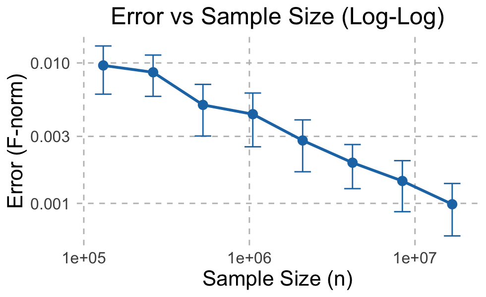
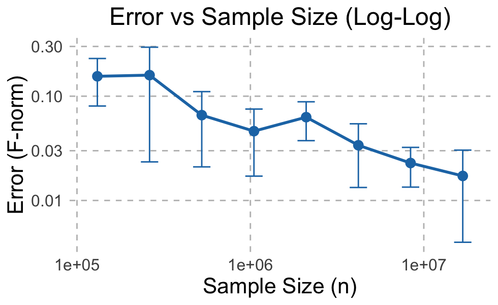
Now we discuss the simulation results. First, as the sample size increases, the log error of the component density exhibits a clear linear decay. Since the error of and has rate with high probability, this experiment confirms the linear relationship between the joint density error and the component density error, as stated in Theorem 14. Notably, in both simulations, the linear independence condition is not required. The superior performance of the conditional i.i.d. model compared to the Bernoulli mixture model can be attributed to its lower number of parameters, and a better separation of the true parameters.
5 Discussion
This paper proposes a high-dimensional nonparametric latent structure model. We introduce an identifiability theorem that unifies existing conditions. In particular, we demonstrate the increasing dimensionality, coupled with diversity in variables, is beneficial to the identifiability. We also establish a perturbation theory under incoherence and derive a minimax risk bounds for high-dimensional nonparametric density estimation, which add up to quantitative rates of convergence. We also develop a recovery algorithm from an estimator of the joint density, which can successfully recover the component densities under incoherence.
There are also some problems to be further investigated under our model:
-
•
Identifiability conditions. For now, Theorem 7 is built on a -partition of . Such a condition could be replaced by properties only depending on . Besides, the condition is still not necessary.
-
•
Full use of diversity. For large , we estimate the component only using variables. Using more variables could be more beneficial.
Acknowledgment
The authors thank Anru Zhang for helpful discussions at the onset of the project. The authors are also grateful to anonymous reviewers for helpful comments.
References
- AGH+ (14) Animashree Anandkumar, Rong Ge, Daniel Hsu, Sham M. Kakade, and Matus Telgarsky. Tensor Decompositions for Learning Latent Variable Models. Journal of Machine Learning Research, 15(80):2773–2832, 2014.
- AMR (09) Elizabeth S. Allman, Catherine Matias, and John A. Rhodes. Identifiability of parameters in latent structure models with many observed variables. The Annals of Statistics, 37(6A), December 2009.
- BCH (09) Tatiana Benaglia, Didier Chauveau, and David R. Hunter. An EM-Like Algorithm for Semi- and Nonparametric Estimation in Multivariate Mixtures. Journal of Computational and Graphical Statistics, 18(2):505–526, January 2009.
- BCH (11) Tatiana Benaglia, Didier Chauveau, and David R. Hunter. Bandwidth Selection in an EM-Like Algorithm for Nonparametric Multivariate Mixtures. In Nonparametric Statistics and Mixture Models, pages 15–27, The Pennsylvania State University, USA, January 2011. WORLD SCIENTIFIC.
- BCMV (14) Aditya Bhaskara, Moses Charikar, Ankur Moitra, and Aravindan Vijayaraghavan. Smoothed analysis of tensor decompositions. In Proceedings of the Forty-Sixth Annual ACM Symposium on Theory of Computing, STOC ’14, page 594–603, New York, NY, USA, 2014. Association for Computing Machinery.
- BCV (14) Aditya Bhaskara, Moses Charikar, and Aravindan Vijayaraghavan. Uniqueness of tensor decompositions with applications to polynomial identifiability. In Maria Florina Balcan, Vitaly Feldman, and Csaba Szepesvári, editors, Proceedings of The 27th Conference on Learning Theory, volume 35 of Proceedings of Machine Learning Research, pages 742–778, Barcelona, Spain, 13–15 Jun 2014. PMLR.
- Bha (97) Rajendra Bhatia. Matrix Analysis. Number 169 in Graduate Texts in Mathematics. Springer, New York, NY, 1997.
- Bir (83) Lucien Birgé. Approximation dans les espaces métriques et théorie de l’estimation. Zeitschrift für Wahrscheinlichkeitstheorie und verwandte Gebiete, 65:181–237, 1983.
- BJR (16) Stéphane Bonhomme, Koen Jochmans, and Jean-Marc Robin. Estimating multivariate latent-structure models. The Annals of Statistics, 44(2), April 2016.
- Che (95) Jiahua Chen. Optimal Rate of Convergence for Finite Mixture Models. The Annals of Statistics, 23(1), February 1995.
- CHL (15) Didier Chauveau, David R. Hunter, and Michael Levine. Semi-parametric estimation for conditional independence multivariate finite mixture models. Statistics Surveys, 9(none), January 2015.
- CX (98) Guoliang Chen and Yifeng Xue. The expression of the generalized inverse of the perturbed operator under Type I perturbation in Hilbert spaces. Linear Algebra and its Applications, 285(1-3):1–6, December 1998.
- FL (23) Zhiyuan Fan and Jian Li. Efficient Algorithms for Sparse Moment Problems without Separation. 36th Annual Conference on Learning Theory, 2023.
- FOS (08) Jon Feldman, Ryan O’Donnell, and Rocco A. Servedio. Learning Mixtures of Product Distributions over Discrete Domains. SIAM Journal on Computing, 37(5):1536–1564, January 2008.
- GGK (90) Israel Gohberg, Seymour Goldberg, and Marinus A. Kaashoek. Singular Values of Compact Operators, pages 96–108. Birkhäuser Basel, Basel, 1990.
- GJM+ (24) Spencer L Gordon, Erik Jahn, Bijan Mazaheri, Yuval Rabani, and Leonard J Schulman. Identification of Mixtures of Discrete Product Distributions in Near-Optimal Sample and Time Complexity. 37th Annual Conference on Learning Theory, 2024.
- GMRS (21) Spencer Gordon, Bijan H Mazaheri, Yuval Rabani, and Leonard Schulman. Source identification for mixtures of product distributions. In Mikhail Belkin and Samory Kpotufe, editors, Proceedings of Thirty Fourth Conference on Learning Theory, volume 134 of Proceedings of Machine Learning Research, pages 2193–2216. PMLR, 15–19 Aug 2021.
- GMSR (20) Spencer Gordon, Bijan Mazaheri, Leonard J. Schulman, and Yuval Rabani. The Sparse Hausdorff Moment Problem, with Application to Topic Models, September 2020. arXiv:2007.08101 [cs, stat].
- GS (22) Spencer L. Gordon and Leonard J. Schulman. Hadamard Extensions and the Identification of Mixtures of Product Distributions. IEEE Transactions on Information Theory, 68(6):4085–4089, June 2022.
- GvdV (01) Subhashis Ghosal and Aad W. van der Vaart. Entropies and rates of convergence for maximum likelihood and Bayes estimation for mixtures of normal densities. The Annals of Statistics, 29(5), October 2001.
- HJ (12) Roger A. Horn and Charles R. Johnson. Matrix analysis. Cambridge University Press, Cambridge ; New York, 2nd ed edition, 2012.
- HK (18) Philippe Heinrich and Jonas Kahn. Strong identifiability and optimal minimax rates for finite mixture estimation. The Annals of Statistics, 46(6A), December 2018.
- HY (20) Roger A. Horn and Zai Yang. Rank of a Hadamard product. Linear Algebra and its Applications, 591:87–98, April 2020.
- HZ (03) Peter Hall and Xiao-Hua Zhou. Nonparametric estimation of component distributions in a multivariate mixture. The Annals of Statistics, 31(1), February 2003.
- JV (02) A Juan and E Vidal. On the use of Bernoulli mixture models for text classiÿcation. Pattern Recognition, 2002.
- JV (04) A. Juan and E. Vidal. Bernoulli mixture models for binary images. In Proceedings of the 17th International Conference on Pattern Recognition, 2004. ICPR 2004., pages 367–370 Vol.3, Cambridge, UK, 2004. IEEE.
- KB (09) Tamara G. Kolda and Brett W. Bader. Tensor decompositions and applications. SIAM Review, 51(3):455–500, 2009.
- KR (83) Richard V Kadison and John R Ringrose. Fundamentals of the theory of operator algebras. Volume I: Elementary Theory. Academic press New York, 1983.
- Kru (77) Joseph B. Kruskal. Three-way arrays: rank and uniqueness of trilinear decompositions, with application to arithmetic complexity and statistics. Linear Algebra and its Applications, 18(2):95–138, 1977.
- KS (14) Hiroyuki Kasahara and Katsumi Shimotsu. Non-parametric identification and estimation of the number of components in multivariate mixtures. Journal of the Royal Statistical Society: Series B (Statistical Methodology), 76(1):97–111, January 2014.
- LHC (11) M. Levine, D. R. Hunter, and D. Chauveau. Maximum smoothed likelihood for multivariate mixtures. Biometrika, 98(2):403–416, June 2011.
- LRA (93) S. E. Leurgans, R. T. Ross, and R. B. Abel. A Decomposition for Three-Way Arrays. SIAM Journal on Matrix Analysis and Applications, 14(4):1064–1083, October 1993.
- LRSS (15) Jian Li, Yuval Rabani, Leonard J. Schulman, and Chaitanya Swamy. Learning Arbitrary Statistical Mixtures of Discrete Distributions, April 2015. arXiv:1504.02526 [cs].
- LW (22) Nan Lu and Lihong Wang. A nonparametric estimation method for the multivariate mixture models. Journal of Statistical Computation and Simulation, 92(17):3727–3742, November 2022.
- PW (25) Yury Polyanskiy and Yihong Wu. Information Theory: From Coding to Learning. Cambridge University Press, 2025.
- RS (80) Michael Reed and Barry Simon. Methods of modern mathematical physics: Functional analysis, volume 1. Gulf Professional Publishing, 1980.
- RSS (14) Yuval Rabani, Leonard J. Schulman, and Chaitanya Swamy. Learning mixtures of arbitrary distributions over large discrete domains. In Proceedings of the 5th conference on Innovations in theoretical computer science, pages 207–224, Princeton New Jersey USA, January 2014. ACM.
- SB (00) Nicholas D. Sidiropoulos and Rasmus Bro. On the uniqueness of multilinear decomposition of n-way arrays. Journal of Chemometrics, 14(3):229–239, 2000.
- SS (90) Gilbert W Stewart and Ji-guang Sun. Matrix perturbation theory. Academic Press, 1990.
- Tei (67) Henry Teicher. Identifiability of Mixtures of Product Measures. The Annals of Mathematical Statistics, 38(4):1300–1302, August 1967. Publisher: Institute of Mathematical Statistics.
- TMMA (18) Behrooz Tahmasebi, Seyed Abolfazl Motahari, and Mohammad Ali Maddah-Ali. On the Identifiability of Finite Mixtures of Finite Product Measures, July 2018. arXiv:1807.05444 [math, stat].
- Tsy (09) Alexandre B. Tsybakov. Introduction to nonparametric estimation. Springer series in statistics. Springer, New York, english ed. edition, 2009.
- VS (19) Robert A. Vandermeulen and Clayton D. Scott. An operator theoretic approach to nonparametric mixture models. The Annals of Statistics, 47(5):2704–2733, October 2019. Publisher: Institute of Mathematical Statistics.
- VS (22) Robert A. Vandermeulen and René Saitenmacher. Generalized Identifiability Bounds for Mixture Models with Grouped Samples, July 2022. arXiv:2207.11164 [cs, math, stat].
- WY (20) Yihong Wu and Pengkun Yang. Optimal estimation of Gaussian mixtures via denoised method of moments. The Annals of Statistics, 48(4), August 2020.
- Yat (85) Yannis G Yatracos. Rates of convergence of minimum distance estimators and kolmogorov’s entropy. The Annals of Statistics, 13(2):768–774, 1985.
- YB (99) Yuhong Yang and Andrew Barron. Information-theoretic determination of minimax rates of convergence. The Annals of Statistics, 27(5):1564–1599, October 1999. Publisher: Institute of Mathematical Statistics.
- ZW (20) Chaowen Zheng and Yichao Wu. Nonparametric Estimation of Multivariate Mixtures. Journal of the American Statistical Association, 115(531):1456–1471, July 2020.
Appendix A Proof in Section 2
A.1 Tensor of Hilbert spaces
We first establish the framework of tensor of Hilbert spaces, here we only introduce the definitions and propositions we need to avoid the ambiguity of notations we need. The proof of classical results are omitted in this subsection, see Chapter 2 of [36, 28] for details.
Let , be two Hilbert spaces with basis and inner product . For , let (also called a simple tensor) be the bilinear form acting on : For ,
| (13) |
Let be the linear combinations of all bilinear forms. The tensor of Hilbert spaces and , denoted by , is defined by the completion of . It can be verified that (See e.g. Proposition 2 in Chapter 2 of [36]) is a Hilbert space with basis and the following inner product rule:
Under this rule, it can be verified that the inner product of two simple tensors is
| (14) |
Note that the definition of inner product from equation (14) is equivalent to the one defined on the basis, so we will use (14) later on. Now we turn to the tensor product of Hilbert space . By Proposition 2.6.5 in [28], we know that the tensor product is associative in the sense of isomorphism. Thus, is defined as the completion of the span of order- simple tensors , with the inner product
For a Hilbert space , the notation is defined as the -tensor power of , i.e., . In the reminder, the notations should be viewed as the definitions above.
Tensor of Hilbert spaces has a natural isomorphism to the product of Hilbert space , like the unfolding of high order tensor in the Euclidean space. The following classical result reveals the relationship in space (See e.g., Theorem II.10 (a) in [36], also Lemma 5.2 in [43]).
Lemma 16.
For a measurable space , there exists a unitary transform such that for all ,
| (15) |
A.2 Proof of Theorem 7
Before proving Theorem 7, we need to formally define the Kruskal rank:
Definition 17 (Kruskal rank of a matrix).
Let be a real matrix. The Kruskal rank of is defined as the maximum number such that any columns of are linearly independent. Denote the Kruskal rank of by .
Definition 18 (Kruskal rank in Hilbert spaces).
Let . We say is -independent if, for any size- index set , are linearly independent. The Kruskal rank of is the maximum number such that is -independent. Denote the Kruskal rank of by .
The following lemma reduces the analysis of general Hilbert spaces to the associated Gram matrices.
Lemma 19.
Let , and let denote the associated Gram matrix. Then, the Kruskal ranks satisfy .
Proof.
We first prove . By the definition of Kruskal rank, there exist elements in that are linearly dependent. Without loss of generality, assume these are . Partition the Gram matrix into blocks:
where is the submatrix corresponding to the inner products of . Since these elements are linearly dependent, is rank deficient. By the row inclusion property [see 21, Observation 7.1.12], the first columns of are linearly dependent. Thus, .
Next, we prove . By the definition of Kruskal rank, every subset of elements in is linearly independent. Consequently, every principal submatrix of of order has full rank. Applying the row inclusion property again, any columns of are linearly independent. Therefore, . ∎
Proof of Lemma 9.
We prove two cases separately.
Case 1: . We prove is positive definite, which implies . Suppose . Using the factorization , where , , we compute:
This implies . Let , where are columns vectors. Then
Since no zero diagonal entries, and for all .
By Lemma 19, , so are linearly independent. For each , let and project onto the orthogonal complement denoted by . By linear independence, and thus . By construction, and for . Therefore,
Since and by Lemma 19, the vectors are linearly independent. Then, and thus .
Since for , the union of hyperplanes has Lebesgue measure zero. Hence, there exists such that for all . Therefore,
Since are linearly independent, it follows that and thus for . We obtain and conclude that is positive definite.
Case 2: . We prove that every principal submatrix of of order is nonsingular. By the row inclusion property of positive semi-definite matrices [see 21, Observation 7.1.12], this implies every columns of is linearly independent. Let denote an arbitrary principal submatrix of order . Since due to the nonzero diagonals, we have . The Kruskal ranks are inherited by those principal submatrices:
It follows that . Similarly, . The submatrices and are positive semidefinite with no zero diagonals, and their Kruskal ranks satisfy . Since is a matrix of order , Case 1 implies that has full rank. ∎
The following lemma [44, Theorem 5.1] is an adaptation of Kruskal’s theorem in the tensor of Hilbert spaces.
Lemma 20 (Hilbert space extension of Kruskal’s theorem).
Let , , and have Kruskal ranks and , respectively. Suppose that . If , , , and
then there exists a permutation and s.t. and with for all .
Now we are ready to prove Theorem 7.
Proof of Theorem 7.
For two joint probability measure having the form as model (1), suppose with parameters , and satisfies the condition in the statement of Theorem 7. Define the finite measure
Then the Radon-Nikodym derivatives are bounded by , thus for all . As a consequence, the density functions of and with respect to have the form
For simplicity, we will write as if the notation has no ambiguity. We now rearrange and along the partition of :
Now, applying Lemma 16, there exists a unitary transform such that (15) holds. Now, by linearity of we have
and
From we know , thus . We only need to show up to a permutation from . Let for simplicity and for . Similarly, we define and for . From Lemma 19 and Lemma 9, we have the following lower bound for the Kruskal rank of :
where is defined as in (5). Similarly, for and we have . Now from the condition (2), applying Lemma 20 for and , we conclude that there exists a permutation and , such that for all , and
Applying the unitary transform on them, we have
Since are all density functions, we know for all and . Thus, from we know for all as well, which implies for all . Now for any measurable set , , which implies , as desired.
Now it remains to find a such that (3) holds but not identifiable. Here we consider two mixtures of binomial distribution and with , where . We will construct , such that satisfies condition (3), , but by a permutation.
Let and for . Then . For all , let , where is a small constant s.t. .
We first show satisfies (3). From for , we know that is -independent but not -independent. Thus, for and the partition of , we have
Now we show that to complete the proof. For any , suppose , we have
Thus, to show , it suffices to prove
| (16) |
for all . We will prove this by induction with respect to . For (16) holds trivially. Now suppose (16) holds for , we will prove that it also holds for . Consider the generating function
Taking -th order derivatives at both sides of the equation to obtain
Now let , using the induction hypothesis we have
This proves (16), thus . We are done. ∎
Appendix B Proof of Theorem 12
We will first introduce some technical lemmas.
Lemma 21.
Let be density functions such that for all and . Suppose is a density function such that
| (17) |
Then there exists a test function , such that for all ,
Proof.
Suppose has dimension . Let , and let be an orthonormal basis for the orthogonal complement of within . Write as linear combinations of the orthonormal basis :
where and for . It follows from the condition (17) that
We then prove the lemma by the probabilistic method. Let and . It suffices to show that the normalized function satisfies the desired property with strictly positive probability. By definition, and . For a fixed , . Let . Then,
where is a standard Gaussian variable. Applying the union bound yields that
Moreover, since , by Markov inequality, we have . Equivalently, . By the union bound, with probability at least ,
This completes the proof. ∎
For the quantitative rates, we follow the concept of Kruskal rank and define the corresponding eigenvalues for a Gram matrix as follows.
Definition 22 (Kruskal eigenvalue of a Gram matrix).
Let be a Gram matrix with. For , the -th Kruskal eigenvalue of is defined as:
where is the principal submatrix of indexed by the set .
Evidently, if and is the associated Gram matrix, then implies . We now present a lemma that establishes a lower bound for the Kruskal eigenvalue of the Hadamard product of two Gram matrices.
Lemma 23.
Suppose are Gram matrices. Then for , then
Proof.
Suppose , where , . Then . Let denote the Khatri-Rao product. Then . Consequently,
where is the submatrix containing the columns of indexed by . Applying [6, Lemma 20], we have
The proof is completed. ∎
Lemma 24.
Consider a Hilbert space with . Let satisfy . Suppose and . Then
Proof.
Without loss of generality, assume . Let . We decompose along and its orthogonal complement as
where and . Then, We obtain
By triangle inequality, . By Cauchy-Schwarz inequality, and . It follows that
| (18) |
It remains to lower bound and . Since , we have
Furthermore, by triangle inequality,
Since , we have . The conclusion follows from (18). ∎
Lemma 25 ([15] Corollary 1.6).
Suppose are two Hilbert spaces, and are two finite rank operators with rank . Denote the singular values of by and , respectively. Then we have
Now we are ready to prove Theorem 12.
Proof of Theorem 12.
For , let and denote the marginal densities of and with respect to the variables indexed by , respectively. Let and . From Cauchy-Schwarz inequality, we have
Thus, we only need to prove the result for .
We begin with some preliminary preparations. From , we know for every and . Thus, applying a unitary transformation , we map to , respectively, with the following explicit form:
We consider the following transform: For , we write the mode- multiplication of as
| (19) |
Then, applying a unitary transformation , we unfold to the following linear operator:
| (20) |
where
, and is the adjoint operator of .
Similarly, we map to .
Note that are both unitary and therefore preserves the inner product, we deduce that , .
Additionally, we have the following relation:
| (21) |
Thus, . Note that are both finite rank linear operators with rank at most . By Lemma 25, we have
| (22) |
Now we show that in (20), are well conditioned as finite rank linear operators, which allows us to focus on the diagonal matrix afterwards. Iteratively applying Lemma 23 with , we have a lower bound of the -th singular value of :
| (23) |
where is the Gram matrix of . The last inequality is due to the fact that and the incoherence condition. Similarly, .
We prove Theorem 12 by contradiction, showing that it conflicts with equation (22) for some and . The proof is divided into the following four steps.
Step 1: Find a component density close to the true one: Define . We show that for any , there exists such that for every ; Without loss of generality, we show this for . From Cauchy-Schwarz inequality, we have and thus . From the assumption on , we can verify . Thus, by Lemma 24, it suffices to show .
Suppose on the contrary there exists some such that for all , Consequently, for all . By Lemma 21, there exists with such that
| (24) |
Thus, the diagonal matrix has a zero diagonal entry, which implies that . On the other hand,
| (25) |
Thus, we obtain
a contradiction to (22).
Step 2: Verify the mapping is one-to-one. We will show that the mapping in Step 1 is one-to-one for every , thus a permutation. Suppose this is not true, then there exists and , such that . Without loss of generality, take . For and -incoherent with them, applying Lemma 21, there exists a with , such that
| (26) |
Since , we know
Similarly, . Consequently, , whereas . Similar to Step 1, we deduce that
a contradiction to (22). The last inequality is from the assumption on . This proves that is an injection from to , thus a permutation.
Step 3: Show that the permutations are identical. We will prove that . Suppose on the contrary there exists such that ; without loss of generality, we take . From , there exists such that ; without loss of generality, we take . From the triangle inequality, we have
Similarly,
Let . From the triangle inequality and , we deduce that
Since are -incoherent, by applying Lemma 21 again, there exists with such that
Let denote the mode- multiplication of a tensor. For , define , respectively. Then . From and the choice of , we obtain
and
By applying a unitary transform, we unfold to
where , and . Similarly, denote the image of by . Similar to (22), we have
From Lemma 23 again, we have . Since has rank at most , we obtain for any . Thus, choosing , we obtain
which leads to a contradiction.The last inequality follows from the assumption on . This proves ’s are identical.
Step 4: Bounding the error of mixing proportion. For the remainder of this proof, we assume is identity without loss of generality. In this step, the norm refers to the operator norm if not specified. We consider the marginal density on the first variables:
| (27) |
where , a rank- linear operator from m to . Similarly, we define and from . Let , and . We have
Since are both rank-, by Lemma 25, .
Appendix C Proof of Theorem 13
C.1 Definitions and some preparations
For Hölder class, we give a formal definition for the Hölder smooth function in the main text:
Definition 26.
For a parameter , where , we say a function is -Hölder smooth with parameter , if is -times continuously differentiable, and the -th derivative satisfies
Now we review some classical results about metric entropy we need for the proof. We begin from the concept of metric entropy.
Definition 27 (covering and packing entropy).
Let be a class of densities and be a metric.
-
1.
An -packing of with respect to is a subset such that for all . The -packing number of is defined to be the maximum number such that there exists a -packing with cardinality .
-
2.
An -net of with respect to is a set such that, for all , there exists such that . The -covering number is defined to be the minimum such that there exists a -net with cardinality .
The -covering entropy and -packing entropy are defined as the logarithm of -covering number and -packing number, respectively.
For a class and a metric , there is a well known relationship between covering and packing number [see e.g. 35, Theorem 27.2]:
| (29) |
There is a close relationship between the entropy of class and the minimax risk. For the minimax upper bound, we have the following classical results from [46, 8]:
Proposition 28.
For and a class of density , given a random sample , we have entropic minimax upper bounds:
We can also derive the minimax lower bound from the bounds of metric entropy. The fundamental work of this characterization is from [47].
Proposition 29 (Theorem 1 in [47]).
Let be KL-divergence between and . The KL -covering number for a class of densities is defined by
Define the covering radius of to be the solution of the following equation:
| (30) |
Suppose we are given a random sample . Then, for any metric with triangle inequality, the minimax risk has a lower bound :
| (31) |
where is defined by the equation
| (32) |
For calculating the cardinality of a packing set, we use the following result.
Proposition 30 (Gilbert–Varshamov bound).
Let . For , define the Hamming distance of to be
Let be a -packing of with respect to Hamming distance. Then for ,
C.2 Entropic bounds
We will first prove the following entropic bounds.
Lemma 31.
Let denote the class of all -Hölder smooth densities on with smoothness parameter and constant . Let be defined as in (11). Then we have
Proof of Lemma 31.
Upper bound: We first prove the entropic upper bound under TV. Pick a -covering of under TV, denoted by . Also, pick a -covering of the simplex , denoted by . We consider the following set:
We now prove that is indeed an -covering of . For any , there exists an element in such that
By triangle inequality, we have (all integral is under Lebesgue measure)
| (33) |
For all , we have the following relation:
Combining this with (33), we have . Thus is an -covering of . Now we calculate the cardinality of :
| (34) |
The inequality is from the classical result about covering number of a simplex (see e.g., Lemma A.4 in [20]). From the entropic bound of 1-dimensional Hölder class, we have [see e.g., 35, Theorem 27.14]
| (35) |
Thus, plug (35) into (34) we have
which proves the TV upper bound.
Now we prove the upper bound under . The idea of choosing a covering set is similar. Pick an -covering of under , and an -covering of under TV, denoted by . The covering set is defined as
Now we prove is an -covering. For , we pick the element in such that
Then we can upper bound :
The first inequality uses the triangle inequality of as a distance, the second uses the Cauchy-Schwarz inequality, the third uses the convexity of Hellinger distance and . Now we bound :
The last inequality is due to for . Thus, .
Now we calculate the cardinality of . Similar to (34), we have
| (36) |
Moreover, has an upper bound given by the entropic bounds of Hölder class [see 35, equation (32.56)]:
| (37) |
Thus, plug (37) into (36) we have the entropic upper bound
as desired.
Lower bound: We first prove the lower bound under TV. For , let be a subset of such that
| (38) |
For every , pick a -packing of , denoted by . We consider the following class:
We write for . Let , and . Now we consider the following packing set:
where is defined as in Proposition 30. Clearly .
Now we show that is an -packing of . We first consider the lower bound of for . Let . Since there exists a such that . Without loss of generality, take . We obtain
| (39) |
The first inequality is from . The second inequality is due to are different elements in the packing set .
For two different elements , the index and are two distinct elements in . Thus, there exists , such that for , . This implies . From (39), we deduce that
Hence, is an -packing of . Now we calculate the cardinality of , given by . Applying Proposition 30, we obtain
Applying the inequality , we have
| (40) |
We have the following lower bound for :
| (41) |
The last inequality is from the entropic bound of 1-dimensional Hölder class [see e.g., 35, Theorem 27.14]. Plugging (41) into (40), we have
This completes the proof of entropic lower bound for TV.
Now we turn to the lower bound for . We pick an -packing of in (38), denoted by . Let . We consider the following set:
where is defined as in Proposition 30. We write and let . Now we construct the packing set to be
| (42) |
We now prove is an -packing. For two different elements , there exists , such that for all , . Thus, we have the lower bound of Hellinger distance:
| (43) |
For two distinct elements , there exists , such that for all , . From (43) we deduce that
| (44) |
This proves that is -packing. Now we calculate the cardinality of , given by Similar to (40), we have
This implies
| (45) |
The last inequality is given by the entropic bounds of Hölder class [see 35, equation (32.56)]. ∎
C.3 Wrapping up the proof
Proof of Theorem 13.
The upper bound in Theorem 13 is directly from Proposition 28. Let be an upper bound of the -covering entropy under , for , we have
Let to get the minimax upper bound for . To guarantee , we need . Similarly, we can derive the minimax upper bound for TV. We omit the details here.
| (46) |
Then, and thus
We will calculate the covering radius of defined in Proposition 29. Now we pick an KL -covering of , denoted by . We consider the following set:
We will now show that is an KL -covering of . For any , we find an element such that . From the additivity of KL-divergence for product density, we have
This shows that
| (47) |
Now we derive an upper bound for KL covering entropy of . We claim that the density class has a finite radius:
This can be verified by choosing the density of uniform distribution on :
Thus, by Theorem 32.6 in [35] with , we have
Combining this with (47), we have
where satisfies . Now we calculate covering radius of . We know for , thus
which gives . Now we apply Proposition 29 to obtain the minimax lower bound. From Lemma 31 we know
Now, plug this and the formula of into (32), we have
This proves the minimax lower bound under . For TV, from Lemma 31 again,
Thus,
∎
Appendix D Details in Section 4
D.1 Recovering the component from the exact joint density
In this subsection, we present the recovery procedure from the known joint density and discuss its connection to Algorithm 1. The joint density can be expressed as
| (48) |
where and . Integrating over , we obtain
| (49) |
Applying a unitary transformation , we map to the following linear operator:
| (50) |
where and . Since is a finite rank operator, we can perform its singular value decomposition (SVD):
| (51) |
where are orthonormal and . Since are -incoherent hence pairwise distinct, and both have full column rank, implying that the diagonal entries of are positive. Let denote the Moore-Penrose inverse of , given explicitly by
| (52) |
We now select a subset of the support of the -th variable and define the operator
| (53) |
where with for . We have the following result.
Lemma 32.
Proof.
Lemma 32 shows that ’s are eigenfunctions of . Consequently, simultaneously diagonalizes for any choice of . In practice, instead of working directly with , we compute its coefficient matrix under the basis :
| (54) |
Let be the matrix whose columns are the eigenvectors of . Then represents the coefficients of under the basis . Thus,
| (55) |
We summarize the above procedure in Algorithm 2 below.
Finally, note that Algorithm 1 in the main text is simply a plug-in version of Algorithm 2.
D.2 Proof of Theorem 14
We need the following perturbation lemmas. The first one is for eigenvectors, and the second is for pseudo inverse of linear operators.
Lemma 33 (Theorem 2.8 in [39]).
Let be a diagonalizable real matrix with eigen decomposition . Rewrite the decomposition as the following:
where and . Then for , we have
| (56) |
where is an absolute constant.
Lemma 34 (Theorem 2 in [12]).
Let be Hilbert spaces and be two linear operators from to . Suppose such that . Then
| (57) |
Proof of Theorem 14.
In this proof, the norm refers to operator norm if not specified. The notation, if not followed by the name of the variable, should be understood as elements in the tensor of Hilbert spaces, like the relationship between and in (49), (50). The operator norm in the tensor of Hilbert spaces is identical to norm in the function space, because the transform between the two spaces is unitary.
We write , such that
| (58) |
Let . We can obtain that is close to in (50):
| (59) |
The first inequality is due to the triangle inequality, the second due to the choice of and the fact that is rank . Now from Cauchy-Schwarz inequality, we bound the right-hand side of (59):
| (60) |
Thus . The -th singular value of is lower bounded from the equation (50) and (23):
| (61) |
From the condition in Theorem 14, we have . Thus, from Lemma 25 we have
| (62) |
Now we apply Lemma 34 to obtain
| (63) |
Let . Now we calculate the error between and in (53). From Cauchy-Schwarz inequality again, we have
| (64) |
Moreover, is upper bounded by a constant since all are upper bounded by . From (63) and (D.2), we can now give an error upper bound for the object of eigen decomposition :
| (65) |
Let , next we need to upper bound the error of in (51) and . From (59), we have . Now, from Davis-Kahan Sin theorem (see e.g., Theorem VII.3.2 in [7]), we have
Thus, we have
| (66) |
Now we can upper bound the error between in (54) and :
| (67) |
Now we are ready to upper bound the error between and in (55). In (55), we know and are both full column rank, thus is invertible. We now write the eigen decomposition of true :
| (68) |
where and . We know . Thus, applying Lemma 33 combined with (D.2) we have
| (69) |
for some constant . Now, let be the functions in (55), for a constant we have
The condition of in Theorem 14 ensures the condition of Lemma 24. Suppose is upper bounded by a constant . We apply Lemma 24 to obtain
where is defined in equation (48). Now, since is on , we do the integral and apply Cauchy-Schwarz to obtain
Now plug in the lower bound of in (61) to obtain the result as desired. ∎