Scalable Spatiotemporal Inference with Biased Scan Attention Transformer Neural Processes

Abstract

Neural Processes (NPs) are a rapidly evolving class of models designed to directly model the posterior predictive distribution of stochastic processes. While early architectures were developed primarily as a scalable alternative to Gaussian Processes (GPs), modern NPs tackle far more complex and data hungry applications spanning geology, epidemiology, climate, and robotics. These applications have placed increasing pressure on the scalability of these models, with many architectures compromising accuracy for scalability. In this paper, we demonstrate that this tradeoff is often unnecessary, particularly when modeling fully or partially translation invariant processes. We propose a versatile new architecture, the Biased Scan Attention Transformer Neural Process (BSA-TNP), which introduces Kernel Regression Blocks (KRBlocks), group-invariant attention biases, and memory-efficient Biased Scan Attention (BSA). BSA-TNP is able to: (1) match or exceed the accuracy of the best models while often training in a fraction of the time, (2) exhibit translation invariance, enabling learning at multiple resolutions simultaneously, (3) transparently model processes that evolve in both space and time, (4) support high dimensional fixed effects, and (5) scale gracefully – running inference with over 1M test points with 100K context points in under a minute on a single 24GB GPU.

1 Introduction

While early Neural Processes (NPs) np ; cnp focused primarily on the posterior predictive of 1D Gaussian Processes (GPs) and simple data distributions like MNIST, many modern NPs tackle far more complex and data hungry distributions spanning geology, epidemiology, climate, and robotics geoai ; stgnp ; convcnp_env ; convcnp_env_2 ; anp_robotics . Furthermore, these tasks often require synthesizing on and off-grid data. Indeed, one of the most recent foundation models for climate, Aardvark aardvark , is a NP that synthesizes temperature, pressure, wind, humidity, and precipitation from on and off-grid data to generate forecasts that outperform traditional numerical weather prediction systems at one thousandth the computational cost.

As NPs grow in scope, there are two competing pressures: scale and accuracy. Scale is particularly salient for applications involving high resolution sensor data, e.g. satellite imagery or LiDAR points clouds. On the other hand, many of these predictions need to be locally accurate to be actionable, e.g. city-level disaster preparedness and vaccine distribution. NPs should be simple, extensible, and computationally tractable to enable widespread use across domains with limited resources. Accordingly, we propose BSA-TNP, a model that effectively balances these desiderata. Our contributions include:

• The Kernel Regression Block (KRBlock): a simple, stackable transformer block that is parameter efficient, sharing weights for query and key updates, and easily extensible, supporting an arbitrary number of attention biases derived from subsets of input features, e.g. space, time, and fixed effects.

• Group invariant (G-invariant) attention biases: we present a general form of attention bias based on group invariant actions that operate on subsets of model input that enable specifying constraints similar to Bayesian priors. For spatiotemporal applications, we focus on translation invariance as a special case and demonstrate that this not only accelerates convergence, but also improves performance and generalization across locations and resolutions.

• Biased Scan Attention (BSA), a novel memory-efficient attention mechanism that accommodates custom, high performance bias functions through compiled JAX functions.

Together, these architectural choices allow BSA-TNP to: (1) match or exceed the accuracy of the best NP models while often training in a fraction of the time, (2) exhibit translation invariance, enabling learning at multiple resolutions simultaneously, (3) transparently model processes that evolve in both space and time, (4) support high dimensional fixed effects, and (5) scale gracefully – running inference on over 1M test points with 100K context points in under a minute on a single 24GB GPU.

2 Background

2.1 Neural Processes

NPs were originally developed as scalable alternatives to exact GPs, which scale $\mathcal{O}(n^{3})$ in time and $\mathcal{O}(n^{2})$ in space. NPs fall into two primary categories: Conditional Neural Processes (CNPs) and Latent Neural Processes (LNPs) np ; cnp . CNPs deterministically encode observed, or “context,” points into a fixed representation, $\mathbf{r}_{c}=f_{\text{enc}}(\mathbf{s}_{c},\mathbf{f}_{c})$, and decode that fixed representation at test locations to retrieve functional output parameters, $\theta_{t}=f_{\text{dec}}(\mathbf{r}_{c},\mathbf{s}_{t})$. CNPs assume the test points factorize conditional on the fixed representation $\mathbf{r}_{c}$, i.e. $p(\mathbf{f}_{t}\mid\mathbf{s}_{c},\mathbf{f}_{c},\mathbf{s}_{t})=\prod_{i}p(\mathbf{f}_{t}^{(i)}\mid\mathbf{s}_{t}^{(i)},\mathbf{r}_{c})$, and are trained to maximize the log-likelihood of the data under the predicted distribution.

LNPs introduce a latent variable $\psi_{c}$, which parameterizes a latent distribution that is sampled and then decoded, i.e. $\psi_{c}=f_{\text{enc}}(\mathbf{s}_{c},\mathbf{f}_{c})$, $\mathbf{z}_{c}\sim q(\mathbf{z}\mid\psi_{c})$, and $\theta_{t}=f_{\text{dec}}(\mathbf{z}_{c},\mathbf{s}_{t})$, theoretically enabling them to better encode global stochastic behavior np , although in practice they tend to perform worse than their conditional counterparts. LNPs are trained by maximizing an evidence lower bound (ELBO).

2.2 Transformer Neural Processes

Transformer Neural Processes (TNPs) tnp are a subclass of CNPs that have recently dominated the NP landscape in terms of accuracy and uncertainty calibration. Most transformers consist of an embedding layer, several transformer blocks, and a prediction head. Transformer blocks typically consist of multi-headed attention followed by a feedforward network, interspersed with residual connections. The attention mechanism attention was inspired by information retrieval tasks and projects its input into three distinct matrices corresponding to queries ($\mathbf{Q}$), keys ($\mathbf{K}$), and values ($\mathbf{V}$). The queries are matched against keys using a kernel, $\mathcal{K}$, and the resulting scores are used as weights for combining the associated values. The most common attention kernel is the dot-product softmax kernel, i.e. $\mathcal{K}(\mathbf{Q},\mathbf{K})\mathbf{V}\coloneqq\text{softmax}(\mathbf{QK}^{\intercal}/\sqrt{d_{k}})\mathbf{V}$ where $d_{k}$ is the embedding dimension of keys.

Unlike other CNPs which typically follow an encode-decode framework, test points are often passed to TNPs alongside context points and allowed to interact with internal representations of context points at multiple levels within the transformer (see Figure 1).

2.3 Scaling Attention

Conventional attention mechanisms have a space and time complexity of $\mathcal{O}(n^{2})$, which presents a challenge as the number of tokens, $n$, increases. There are five broad categories of research that attempt to address this: (1) sparsity sparse ; longformer ; bigbird ; reformer ; sinkhorn , (2) inducing points perceiver ; settransformer , (3) low-rank approximations linformer ; performer ; efficient , (4) reuse or sharing lazyformer ; reusetransformer , and (5) optimized memory and / or hardware code memory_efficient_attention ; flash1 ; flash2 ; flash3 ; flex .

Most contemporary NPs, such as Latent Bottlenecked Attentive Neural Processes lbanp , Memory Efficient Neural Processes via Constant Memory Attention Blocks cmab , (Pseudo Token) Translation Equivariant Transformer Neural Processes pttnp , and Gridded Transformer Neural Processes gridtnp , focus on (2) inducing points and use some form of Perceiver or Set Transformer attention perceiver ; settransformer , which introduce a number of latent (inducing) tokens, $k$, which is often much smaller than either the number of context points, $n_{c}$, or test points, $n_{t}$. While inducing points enable more scalable training, they introduce additional complexities, such as choosing the number of latents as well as their locations, which in turn determine the accuracy of model output. For this reason, BSA-TNP targets category (5), memory-efficient attention (see subsection 4.3).

2.4 Attention Bias

Attention bias, $\mathbf{B}$, injects domain knowledge into the kernel and takes the following form:

$$\mathcal{K}(\mathbf{Q},\mathbf{K})\mathbf{V}\coloneqq\text{softmax}(\mathbf{QK}^{\intercal}/\sqrt{d_{k}}+\mathbf{B})\mathbf{V}$$ (1)

Graph Neural Networks often leverage attention bias to encode graph topology at various scales, e.g. the Graphormer graphormer encodes spatial and structural biases using the shortest path and node centrality statistics. Similarly, in large language modeling (LLM), Press et al. introduced Attention with Linear Biases (ALiBi) alibi , which replaces positional embeddings with a bias that is proportional to the distance between tokens, i.e. $b(i,j)=-m\cdot|i-j|$ where $m$ is a fixed or learnable scalar and $i$ and $j$ are token positions. ALiBi matches the performance of sinusoidal embeddings while allowing the model to extrapolate far beyond its training range.

Adopting a Bayesian perspective, attention bias can be conceptualized as a log-prior over keys. That is, if we accept the following analogy $p(i\text{ attends to }j)\coloneqq p(j\mid i)\propto\exp(\mathbf{q}_{i}^{\intercal}\mathbf{k}_{j})\exp(\mathbf{b}_{ij})$, we can see that $\log p(i\text{ attends to }j)\propto\mathbf{q}_{i}^{\intercal}\mathbf{k}_{j}+\mathbf{b}_{ij}$. When performing inference on spatiotemporal processes—such as with Hamiltonian Monte Carlo—it is standard practice to use a prior that encodes the strength of association between spatial random effects. According to Tobler’s First Law of Geography: “everything is related to everything else, but near things are more related than distant things” tobler1970computer . These priors can be important not only for convergence but also for enforcing domain knowledge about a particular process, e.g. a sick person cannot infect a healthy one 10 miles away when she sneezes. While purely analogic, this insight suggests how we might encode a similar prior for spatiotemporal phenomena through attention bias, mirroring the covariance-based approaches common in spatial statistics.

3 Group Invariance

Learning meaningful functions from limited data is fundamentally challenging without strong inductive biases. In the context of NPs, the absence of structural assumptions forces the model to search over a large and unconstrained hypothesis space, which can lead to poor generalization and extrapolation. This problem is particularly pronounced when the target function exhibits symmetries that the model does not exploit.

One principled way to address this issue is to encode known invariances – transformations that leave the data distribution unchanged – directly into the model. Invariances constrain the model’s behavior to be consistent with symmetries in the data, effectively reducing the hypothesis space and guiding learning toward solutions that generalize better. For NPs, incorporating such structure can accelerate convergence, increase accuracy, and improve generalization (see section 5).

Encoding invariances in NPs have been studied theoretically and empirically in the context of translation-invariant models. In particular, pttnp show that when the underlying stochastic process is stationary—meaning its distribution is invariant to translations—translation-invariant NPs can achieve improved predictive performance and uncertainty calibration. Formally, we define:

Definition 1.

A stochastic process $F(s)$, $s\in S=\mathbb{R}^{d}$ is said to be stationary if all its finite-dimensional marginal distributions are translation invariant. That is, the equality in distribution

$$\left(F(s_{1}),\ldots,F(s_{k})\right)\stackrel{{\scriptstyle d}}{{=}}\left(F(s_{1}+\tau),\ldots,F(s_{k}+\tau)\right)$$

holds for all $k\in\mathbb{N}$, $s_{1},\ldots,s_{k}\in S$, and $\tau\in S$ and $\stackrel{{\scriptstyle d}}{{=}}$ signifies equality in distribution.

This notion of stationarity can be extended to a broader class of symmetries by considering a group $G$ acting on the input space $D$. The space $D$ may include not only spatial coordinates, but also temporal indices, fixed effects, or other structured covariates. Such a generalization allows us to capture invariances beyond translations—such as rotations, time shifts, scaling transformations, or permutations of categorical attributes—depending on the structure of $G$ and its action on $D$.

Let $\mathbin{\bm{\cdot}}:G\times D\rightarrow D$ be a group action, written as $g\mathbin{\bm{\cdot}}d$ for $g\in G,d\in D$, extending the notion to tuples over $D$ by applying the action element-wise.

Definition 2.

A function $f$ over $D$, is $G$-invariant if $f(g\mathbin{\bm{\cdot}}\mathbf{d})=f(\mathbf{d})$ for all $\mathbf{d}\in D^{k}$ and $g\in G$.

Definition 3.

A stochastic process $F$ is $G$-stationary if all its finite dimensional marginal distributions are $G$-invariant, that is $F(\mathbf{d})\stackrel{{\scriptstyle d}}{{=}}F(g\mathbin{\bm{\cdot}}\mathbf{d})$ holds for all $\mathbf{d}\in D^{k}$ and $g\in G$.

For instance, consider modeling household income distributions across different countries. While absolute income levels may vary, the shape of the distribution may remain consistent up to a multiplicative scaling factor. In this case, the process may be invariant under group actions that rescale income. Likewise, in panel data settings where observations are indexed by individual IDs and time, a process may be invariant to permutations over individuals, corresponding to a permutation group acting on a categorical component of $D$.

To understand how $G$-invariance can be incorporated into an NP, we examine the structure of the posterior predictive map $\pi\colon(\mathbf{d}_{c},\mathbf{f}_{c},\mathbf{d}_{t})\mapsto(F(\mathbf{d}_{t})\mid F(\mathbf{d}_{c})=\mathbf{f}_{c})$. This map captures the conditional distribution that an NP aims to approximate. The following result, which generalizes the theorem from pttnp beyond translations to arbitrary group actions, formalizes the connection between $G$-stationarity of the underlying process and the symmetries of the prediction map:

Theorem 1.

A stochastic process $F$ is $G$-stationary if and only if the posterior predictive map $\pi$ is $G$-invariant with respect to the context and target inputs, i.e., $\pi(g\mathbin{\bm{\cdot}}\mathbf{d}_{c},\mathbf{f}_{c},g\mathbin{\bm{\cdot}}\mathbf{d}_{t})=\pi(\mathbf{d}_{c},\mathbf{f}_{c},\mathbf{d}_{t})$, for all $g\in G$ and all $\mathbf{d}_{c},\mathbf{f}_{c},\mathbf{d}_{t}$.

This result provides a direct prescription for incorporating invariances into NPs: if the model is designed such that its predictive map is $G$-invariant in the inputs, then it correctly reflects the $G$-stationarity of the process it aims to model. The full proof can be found in Appendix G. Since many spatiotemporal tasks exhibit some degree of translation invariance, we focus primarily on that group action, although we provide and example of rotational invariance in Appendix B.

4 Biased Scan Attention Transformer Neural Process (BSA-TNP)

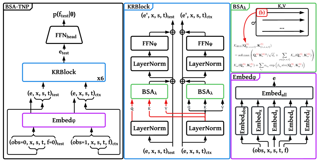
Figure 1: BSA-TNP Overview. The leftmost panel contains the high level architecture (BSA-TNP), the center panel the Kernel Regression Block (KRBlock), and the rightmost panels contain illustrations of Biased Scan Attention (BSA) and the embedding network. Subscripts in block names identify collections of parameters. While KRBlocks and BSA support an arbitrary number feature groups, for the purposes of this paper we divide them into observation status (obs), fixed effects (x), spatial locations (s), and temporal locations $(\mathbf{t})$. Learned embeddings are denoted by (e) and function values by (f). The ctx and test subscripts denote context and test points, respectively.

The Biased Scan Attention Transformer Neural Process (BSA-TNP) architecture consists of an embedding layer, a stack of KRBlocks, and a prediction head (left most panel in Figure 1). Inputs consist of a 5-tuple: observation status (obs), fixed effects (x), spatial locations (s), temporal locations (t), and function values (f). For unobserved test locations, we set f to zero when embedding, similar to other TNP-based architectures tnp ; pttnp . Each feature group is embedded separately and then combined with another network, typically a MLP (bottom right panel in Figure 1). The feature groups that can be used for bias, i.e. (x,s,t), are passed through a residual connection to the KRBlocks. The output of a model is a distribution over test points parameterized by the model output, $p(\mathbf{f}_{\text{test}}\mid\bm{\theta})$.

4.1 Kernel Regression Block (KRBlock)

A Kernel Regression Block (KRBlock) is a generic transformer block inspired by Nadaraya-Watson kernel regression nw_regression , which takes the following form when test points cross attend to context points in NPs (see also red lines in center panel of Figure 1):

$$\begin{split}\mathbf{v}^{(i)\prime}_{\text{test}}=f(\mathbf{q}_{\text{test}}^{(i)};\mathbf{K}_{\text{ctx}},\mathbf{V}_{\text{ctx}})&=\sum_{j}\frac{\mathcal{K}(\mathbf{q}_{\text{test}}^{(i)},\mathbf{k}_{\text{ctx}}^{(j)})}{\sum_{m}\mathcal{K}(\mathbf{q}_{\text{test}}^{(i)},\mathbf{k}_{\text{ctx}}^{(m)})}\mathbf{v}_{\text{ctx}}^{(j)}\end{split}$$ (2)

In BSA-TNP, the queries and keys are extended to include additional terms used for bias (see subsection 4.2), so $\mathbf{q}_{\text{test}}=\mathbf{q}_{\{e,x,s,t\}_{\text{test}}}$ and $\mathbf{k}_{\text{ctx}}=\mathbf{k}_{\{e,x,s,t\}_{\text{ctx}}}$. Inside each block, the learned embeddings (e) are updated but the additional features (x,s,t) are passed unaltered through residual connections. Stacking KRBlocks allows the model to perform iterative kernel regression on increasingly complex internal representations of test and context points. KRBlocks have complexity $\mathcal{O}(n_{c}^{2}+n_{c}n_{t})$ where $n_{c}$ is the number of context points and $n_{t}$ is the number of test points.

4.2 Group-invariant attention bias

BSA-TNP can be configured to be $G$-invariant (see Section 3), as formalized in Theorem 2. For brevity, let $\mathbf{d}=(\mathbf{x},\mathbf{s},\mathbf{t})$ denote the tuple of fixed effects, spatial locations, and temporal indices, and let $\mathbf{d}_{c}$, $\mathbf{d}_{t}$ be the context and target inputs, respectively.

Theorem 2.

BSA-TNP is $G$-invariant in $(\mathbf{d}_{c},\mathbf{d}_{t})$ if both the attention bias functions and the embedding function $\textbf{Embed}_{\bm{\varphi}}$ are $G$-invariant in $(\mathbf{d}_{c},\mathbf{d}_{t})$.

Here, the group action $g\in G$ may act on any subset of components in $\mathbf{d}$, such as scaling household income in (x), rotating spatial coordinates (s), translating time indices (t), or any combination thereof. For example, if $G$ represents temporal translations, then the action is defined as $g\mathbin{\bm{\cdot}}\mathbf{d}=(\mathbf{x},\mathbf{s},g\mathbin{\bm{\cdot}}\mathbf{t})$. The generic form of bias used in BSA-TNP is provided in Equation 3.

$$\mathbf{B}_{ij}=\sum_{\omega\in\{x,s,t\}}\mathcal{K}_{\omega}(\mathbf{q}_{\omega}^{(i)},\mathbf{k}_{\omega}^{(j)})$$ (3)

For the spatiotemporal benchmarks in this paper, we instantiate $G$ as a group of spatial and/or temporal translations in $\mathbb{R}^{d}$. To ensure $G$-invariance under this group, the spatial location (s) or temporal location (t) must be excluded from the initial embedding function, making $\textbf{Embed}_{\bm{\varphi}}$ invariant to spatial and/or temporal shifts. For our bias kernel, $\mathcal{K}_{\omega}$, we use RBF-networks:

$$\mathbf{B}_{ij}^{(h)}=\sum_{\omega\in\{s,t\}}\sum_{f=1}^{F}a_{f}\cdot\exp\left(-b_{f}\|\mathbf{q}_{\omega}^{(i)}-\mathbf{k}_{\omega}^{(j)}\|^{2}\right)$$ (4)

where $h$ denotes the attention head and $\{a_{f},b_{f}\}_{f=1}^{F}$ are learnable parameters for $F$ basis functions. In BSA-TNP, we use $F=5$ for space and $F=3$ for time; in initial tests we found little benefit to using more. Since these biases depend only on pairwise distances between terms, they are translation invariant. By Theorem 2, this ensures that the posterior predictive map is also translation-invariant. A proof for Theorem 2 is provided in Appendix H.

Notably, while G-invariance is most effective for stationary processes, these biases can still prove useful when a process is only partially stationary. For example, when measuring pollution, the distribution is determined both by pollution generation centers as well as the local weather patterns. In this case, it is likely advantageous to embed locations and use spatial attention bias since locations can act as proxies for cities, which have unique pollution profiles, as well as summarize information about local weather patterns, which affect all locations similarly (see subsection 5.4).

4.3 Biased Scan Attention (BSA)

As mentioned previously, when a data distribution exhibits some form of G-invariance, this allows the model to exploit structure and extrapolate beyond the training region. This means that these models can be trained on comparatively small input domains and applied to much larger ones at inference time (see subsection 5.1). Thus, since training can be calibrated to the available compute, this shifts the primary focus to inference.

In spatiotemporal applications, inference is typically performed over a single large region or a small collection of large regions and the primary computational bottleneck is memory. Fortunately, there has been a wave of innovation in memory-efficient attention variants, e.g. memory-efficient attention for TPUs memory_efficient_attention and Flash Attention 1, 2, and 3 for CUDA devices flash1 ; flash2 ; flash3 . There is also FlexAttention flex , which supports many common masking functions and scalar biases. Unfortunatately, none of these variants currently support arbitrary bias functions, which means bias must be omitted or passed as a fully materialized matrix, undermining the memory efficiency. Accordingly, we introduce Biased Scan Attention (BSA), a scan-based memory-efficient attention mechanism that supports arbitrary bias functions that take the form of JIT-compiled JAX functions jax .

BSA largely follows the chunking algorithm defined in Flash Attention 2 flash2 , but adopts the scan-based tiling and gradient checkpointing of memory efficient attention memory_efficient_attention . By using jax.lax.scan with gradient checkpointing, BSA calculates attention scores and custom bias terms on the fly with constant memory. Due to space constriants, we detail the full procedure in Appendix E.

5 Experiments

In this section we evaluate BSA-TNP, Convolutional Conditional Neural Processes (ConvCNP) convcnp , Pseudo Token Translation Equivariant Neural Processes (PT-TE-TNP) pttnp , and the original Transformer Neural Process (TNP-D) tnp on a collection of synthetic and real-world data. The objective of these experiments, which mostly focus on spatiotemporal applications, is to demonstrate the importance of G-invariance, particularly translation invariance in space and time. We demonstrate that BSA-TNP achieves the best accuracy and uncertainty calibration while often requiring less time for training and inference. All models have approximately 500K parameters, except PT-TE-TNP which has approximately 1.8M. We provide detailed parameterizations in Appendix A and model complexity and estimated FLOPs in Appendix C. All experiments were run on a single NVIDIA GTX 4090 24GB GPU.

5.1 2D Gaussian Processes

For this benchmark, we create tasks from 2D GP samples with a squared exponential kernel and lengthscale sampled from $\text{Beta}(3.0,7.0)$, which has a mean and median of $\approx$ 0.3. This is a more challenging benchmark than is typically used and allows for greater differentiation among models since more than 50% of lengthscales fall below 0.3 and less than 10% lie above 0.5. (In practice, we found that even less powerful NPs could easily learn lengthscales above 0.4-0.5). We provide an extensive description of the 2D GP tasks in Appendix B.

In order to evaluate the generalization of various NPs, we evaluate them under four different scenarios: (1) tasks sampled from the training domain, (2) tasks sampled from the training domain shifted by 10, (3) tasks where the domain has doubled along each axis, and (4) tasks where the model receives data at two different scales simultaneously. Scenario (4) is particularly relevant because it mimics a situation where satellite imagery is available at two different levels of granularity and must be synthesized. Multiresolution training is also useful under limited compute: by providing the model with high resolution data for a target region and coarse resolution data for the surrounding area, the model can focus on the target region while still incorporating important contextual information. In this benchmark, using the coarser resolution for surrounding area results in a $\approx$78% reduction in the total number of pixels. Appendix F shows an example of a multiresolution task. Because ConvCNP requires a fixed grid and TNP-D fails under shifting and scaling, we compare only PT-TE-TNP and BSA-TNP on (4). In this case, PT-TE-TNP struggles because it has to allocate a fixed number of latents across the entire domain.

Table 1: 2D GP tasks.

Model	NLL	Shifted NLL	Scaled NLL	Train (min)	Infer (batch/s)
ConvCNP	$-0.22\pm 0.01$	$-0.23\pm 0.00$	$-0.24\pm 0.01$	$121.10\pm 1.02$	$27.56\pm 0.04$
TNP-D	$-0.26\pm 0.00$	$21.32\pm 9.23$	$4.10\pm 0.67$	$65.27\pm 0.04$	$63.95\pm 0.40$
PT-TE-TNP	$0.32\pm 0.02$	$0.32\pm 0.02$	$1.28\pm 0.05$	$72.40\pm 0.08$	$73.35\pm 0.77$
BSA-TNP	$\mathbf{-0.32\pm 0.01}$	$\mathbf{-0.32\pm 0.00}$	$\mathbf{-0.28\pm 0.01}$	$\mathbf{36.98\pm 0.09}$	$\mathbf{103.74\pm 0.43}$

Table 2: 2D GP: Tasks trained on two scales simultaneously. Half of the context points come from $[-0.5,0.5]$ and the other half from $[-1.5,1.5]$, simulating a high resolution target zone with coarser observations from the surrounding area.

Model	NLL	MAE	RMSE	CVG at 95%	Train (min)
PT-TE-TNP	$0.12\pm 0.06$	$0.31\pm 0.01$	$0.48\pm 0.01$	$\mathbf{0.95\pm 0.00}$	$52.40\pm 0.05$
BSA-TNP	$\mathbf{-0.23\pm 0.00}$	$\mathbf{0.25\pm 0.00}$	$\mathbf{0.41\pm 0.00}$	$\mathbf{0.95\pm 0.00}$	$\mathbf{16.23\pm 0.04}$

5.2 Epidemiology

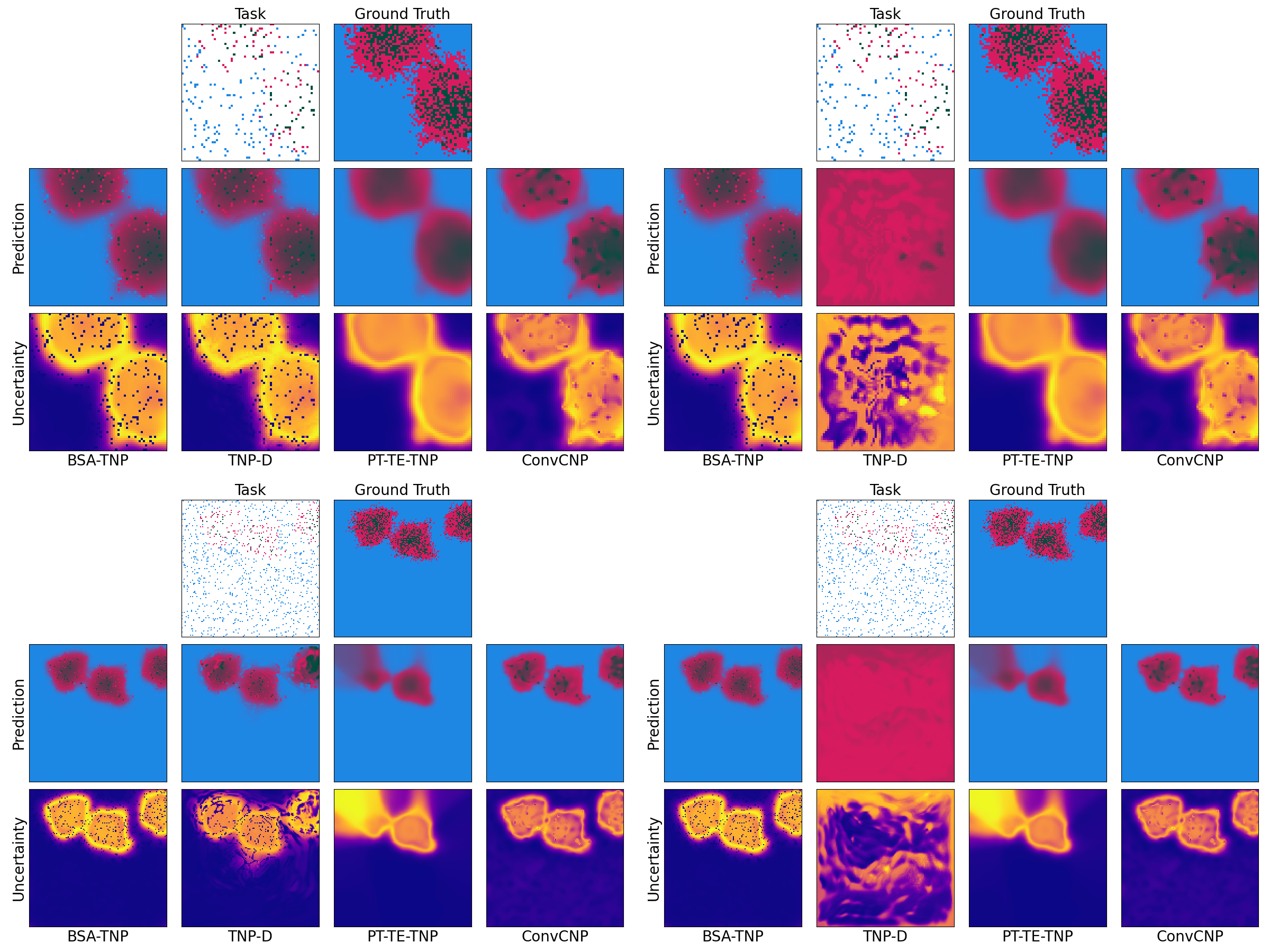
Figure 2: Susceptible-Infected-Recovered (SIR) tasks. Susceptible individuals are represented by blue pixels, infected by magenta, and recovered by green. On the upper left is a task on the training domain $[-2,2]^{2}$. On the upper right is the same task shifted right by 10 to $[8,12]^{2}$. Bottom left is a task where the training domain is doubled along each axis from $[-2,2]^{2}$ to $[-4,4]^{2}$ and increases in resolution from 64x64 to 128x128. The bottom right is the same 128x128 task shifted right by 10 to $[6,14]^{2}$. TNP-D fails under shifts and scaling. PT-TE-TNP fails under scaling since the psuedo-token locations are learned during training; it also fails to reproduce observations of particular individuals due to the bottleneck induced by psuedo-tokens. ConvCNP is able to shift and scale but requires manual modification of the induced grid each time it is applied on a new domain; it also fails to reproduce observations of particular individuals due to the oversmoothing introduced by RBF kernels on the induced grid. BSA-TNP suffers no performance degradation under both shifting and scaling relative to the training domain.

To evaluate performance on an epidemiological application, we generate tasks from the Susceptible-Infected-Recovered (SIR) model, which models the spread of infectious outbreaks. It is governed by an infection rate, $\beta$, a recovery rate, $\gamma$, and the number of initial infections, $\omega$. We sample $\beta\sim\operatorname{Beta}(2,8)$, $\gamma\sim\operatorname{InvGamma}(5,0.4)$, and $\omega\sim\operatorname{randint}(1,5)$. The infection rate, $\beta$, is decreased as an inverse function of distance from the infected individual. In expectation, this parameter setting corresponds to an infection rate of 20% upon exposure and a 10-day recovery period (similar to COVID-19). We train all models on 64x64 images and use the same task distribution as the 2D GP benchmark. A notable difference here is that we train and evaluate models with context points included in the test points. The reason for this is that unlike infections, recoveries are independent of one another. If the model has been told that a particular individual recovered, it should be able to reproduce that in the output, which is is not the case for models that smooth inputs, e.g. PT-TE-TNP and ConvCNP. We provide an illustration of the SIR tasks in Figure 2, and the results are in Table 3.

Table 3: Susceptible-Infected-Recovered (SIR) tasks.

Model	NLL	Shifted NLL	Scaled NLL	Train (min)	Infer (batch/s)
ConvCNP	$0.24\pm 0.00$	$0.24\pm 0.00$	$0.21\pm 0.00$	$119.51\pm 0.30$	$31.93\pm 0.08$
TNP-D	$\mathbf{0.19\pm 0.00}$	$8.26\pm 0.80$	$0.27\pm 0.01$	$51.42\pm 0.40$	$95.10\pm 1.05$
PT-TE-TNP	$0.26\pm 0.00$	$0.26\pm 0.00$	$0.38\pm 0.00$	$60.55\pm 0.28$	$116.54\pm 2.69$
BSA-TNP	$\mathbf{0.19\pm 0.00}$	$\mathbf{0.19\pm 0.00}$	$\mathbf{0.17\pm 0.00}$	$\mathbf{23.60\pm 0.11}$	$\mathbf{225.30\pm 1.98}$

5.3 Climate

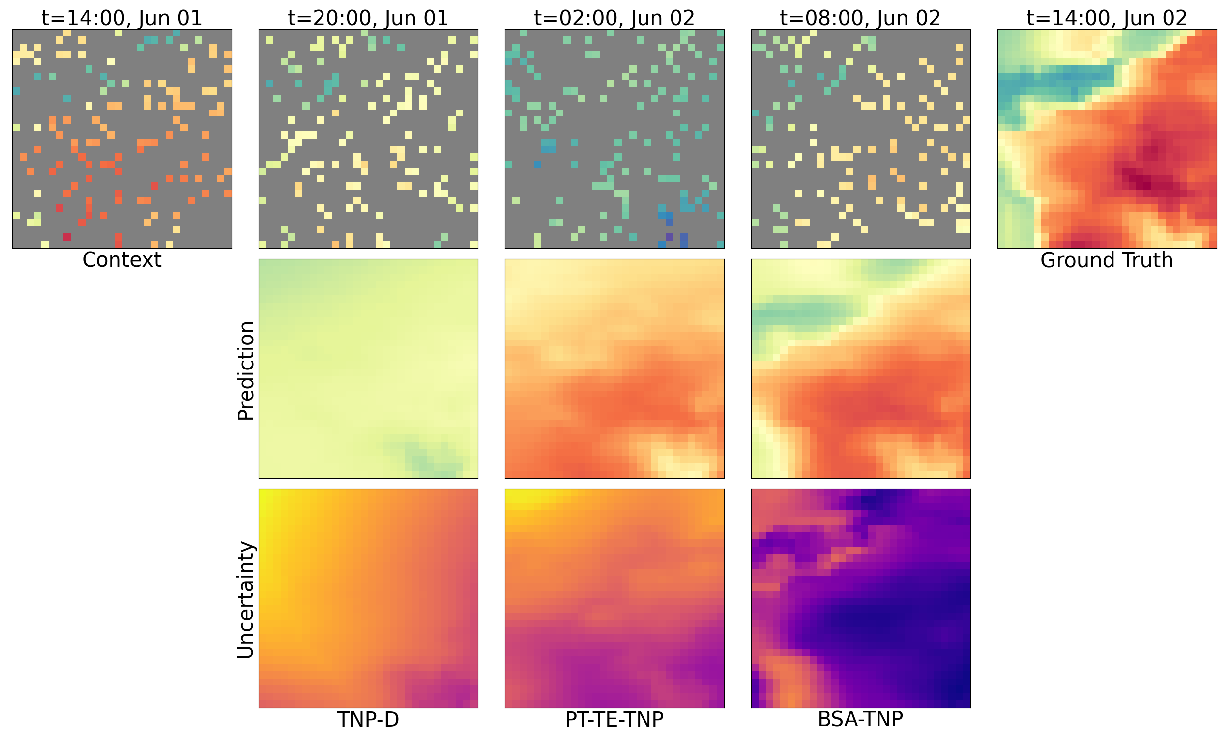
Figure 3: ERA5 ground surface temperature from a sample in northern Europe $[53^{\circ}\mathrm{N},\,63^{\circ}\mathrm{N}]\times[8^{\circ}\mathrm{W},\,28^{\circ}\mathrm{W}]$. Models were trained on central Europe $[42^{\circ}\mathrm{N},\,53^{\circ}\mathrm{N}]\times[8^{\circ}\mathrm{W},\,28^{\circ}\mathrm{W}]$. TNP-D generalizes poorly to this out of domain sample and PT-TE-TNP tends to create an oversmoothed representation. BSA-TNP creates a close approximation and recognizes that the sample from 24H (leftmost context panel) ago is relevant for the current forecast.

For climate, we largely follow the setup in pttnp with ERA5 era5 surface air temperatures. To test learning over time and generalization across space, we train models on tasks from central Europe $[42^{\circ}\mathrm{N},\,53^{\circ}\mathrm{N}]\times[8^{\circ}\mathrm{W},\,28^{\circ}\mathrm{W}]$ and test them on tasks from northern Europe $[53^{\circ}\mathrm{N},\,63^{\circ}\mathrm{N}]\times[8^{\circ}\mathrm{W},\,28^{\circ}\mathrm{W}]$ and western Europe $[42^{\circ}\mathrm{N},\,53^{\circ}\mathrm{N}]\times[-4^{\circ}\mathrm{W},\,8^{\circ}\mathrm{W}]$ over random 30-hour segments of time. When testing on northern Europe, we use western Europe as a validation set and select the best model for testing and vice versa when testing on western Europe. Unlike pttnp which inpaints several frames over time, we change the benchmark to forecast the weather in the next 6 hours. We also add “hour of day” to the feature set and increase the resolution from $0.5^{\circ}$ to $0.25^{\circ}$. The task consists of 4 context frames and 1 test frame, each separated by 6 hours. The inputs we use are x=(elevation, hour of day), s=(latitude, longitude), t=time, f=surface temperature. More details on the experimental setup can be found in Appendix B. Figure 3 provides a visualization of an example task and the results in Table 4 and Table 5 show BSA-TNP outperforms competitors. ConvCNP was excluded from this benchmark because does not natively handle space and time or extra covariates.

Table 4: ERA5 CNW - Training on central, validating on northern, and testing on western Europe.

Model	NLL	MAE	RMSE	CVG at 95%	Train (min)
TNP-D	$1.00\pm 0.06$	$0.35\pm 0.01$	$0.44\pm 0.01$	$0.79\pm 0.01$	$123.35\pm 3.43$
PT-TE-TNP	$0.21\pm 0.03$	$0.22\pm 0.00$	$0.28\pm 0.00$	$0.87\pm 0.01$	$124.88\pm 0.04$
BSA-TNP	$\mathbf{-0.02\pm 0.06}$	$\mathbf{0.18\pm 0.01}$	$\mathbf{0.24\pm 0.01}$	$\mathbf{0.89\pm 0.02}$	$\mathbf{120.25\pm 0.05}$

Table 5: ERA5 CWN - Training on central, validating on western, and testing on northern Europe.

Model	NLL	MAE	RMSE	CVG at 95%	Train (min)
TNP-D	$1.59\pm 0.17$	$0.32\pm 0.02$	$0.40\pm 0.02$	$0.66\pm 0.03$	$\mathbf{114.96\pm 0.08}$
PT-TE-TNP	$0.22\pm 0.02$	$0.22\pm 0.00$	$0.28\pm 0.00$	$0.87\pm 0.01$	$120.13\pm 0.04$
BSA-TNP	$\mathbf{-0.17\pm 0.05}$	$\mathbf{0.16\pm 0.00}$	$\mathbf{0.21\pm 0.00}$	$\mathbf{0.90\pm 0.02}$	$115.48\pm 0.11$

5.4 Partially Stationary Processes

In order to test the effect of our attention bias on a process that is not fully stationary, we use the Beijing Multi-Site Air Quality benchmark from the UCI repository beijing . This dataset measures pollution across 12 cities in China and includes not only location and time, but also windspeed, wind direction, dewpoint, temperature, and rain. We include most of these as fixed covariates, as well as some generated ones including “day of week” and “is weekend.” Table 6 demonstrates that our bias improves performance even when G-invariance is not strictly observed.

Table 6: Beijing Air Quality

Model	NLL	MAE	RMSE	CVG at 95%	Train (min)
TNP-D	$-1.38\pm 0.08$	$\mathbf{0.04\pm 0.00}$	$\mathbf{0.06\pm 0.00}$	$0.87\pm 0.01$	$\mathbf{9.08\pm 0.04}$
PT-TE-TNP	$-1.59\pm 0.06$	$\mathbf{0.04\pm 0.00}$	$\mathbf{0.06\pm 0.00}$	$\mathbf{0.92\pm 0.00}$	$22.70\pm 0.09$
BSA-TNP	$\mathbf{-1.68\pm 0.03}$	$\mathbf{0.04\pm 0.00}$	$\mathbf{0.06\pm 0.00}$	$0.91\pm 0.01$	$12.24\pm 0.05$

6 Limitations and Future Work

While most NP tasks assume sparse observations and dense predictions, some tasks have dense observations and sparse predictions, e.g. video prediction tasks. In this case, BSA-TNP is still has quadratic complexity in the number of context points, making training and inference over a collection of dense frames computationally burdensome. In future work, we hope to extend BSA-TNP to incorporate frame summarizations from models like I-JEPA ijepa to overcome this limitation.

7 Conclusion

In this work, we introduce BSA-TNP which represents a significant step forward in NP design by combining simplicity, scalability, and extensibility with KRBlocks and G-invariant attention biases. Its ability to capture complex spatiotemporal dependencies with minimal overhead not only delivers state-of-the-art accuracy, but also enables inference at scale. And because of its broad applicability, we hope it will form a foundational tool for scientists who work with spatiotemporal phenomena and accelerate research in critical domains like climate, epidemiology, and robotics. We do not anticipate BSA-TNP having any negative societal impacts.

Appendix A Model Parameterizations

ConvCNP:

We use the “off-grid” version of ConvCNP since we train and test on off grid observations for many benchmarks. We use an induced density of 16 points per unit, which corresponds to 64 units per axis for most benchmarks that are trained on $[-2,2]^{2}$. This implies that in a 64x64 image, each pixel has its own grid point. We use ConvDeepSets for encoding and decoding to the latent grid and a stack of 8 ConvCNPNet blocks with kernel size (9, 9) and feature dimension of 128. The prediction head consists of a 4 layer MLP with 3 layers with 128 hidden units and a final layer projecting to the output dimension. This parameterization has $\approx 507K$ parameters, which varies slightly depending on the dimension of inputs and outputs.

TNP-D:

We use the standard formulation defined in [29], which consists of a stack of transformer encoder layers with a special mask to prevent context and test points from attenting to test points. We make a slight digression for the Beijing Multi-City Air Quality and Generic Spatial benchmarks where we modify the transformer blocks to use pre-normalization. We found that TNP-D struggled to learn without this, even though it was not part of the original design. TNP-D has a 3-layer embedding MLP that consists of 256, 128, and 64 units, respectively. It uses 6 transformer encoder blocks each with 4 attention heads. The token embedding dimension is 64 throughout except when performing attention, when we upscale the queries, keys, and values to 128. Feedfoward layers consist of two hidden layers with 256 and 64 units, respectively. The prediction head is identical to feedforward layers except it has an additional layer projecting to the output dimension. This parameterization results in $\approx$477K parameters, which varies slightly depending on the dimension of inputs and ouputs. We parameterize BSA-TNP in almost an identical fashion to maintain as much parity as possible.

PT-TE-TNP:

We follow the default parameterization from the github repo associated with [2]. We use the IST-based architecture, as the authors noted this performed better in their tests. The model uses a token dimension of 128, 8 attention heads, 5 stacked PT-TE-IST blocks, and 32 pseudo-tokens. This parameterization results in $\approx$ 1.85M parameters, which varies slightly depending on the dimension of inputs and outputs.

BSA-TNP:

We use 6 KRBlocks, 4 attention heads, and a token embedding of 64. We upscale this to 128 when performing attention, similar to TNP-D. Also like TNP-D, we use 3-layer embedding MLP that consists of 256, 128, and 64 units, respectively. Feedfoward layers consist of two hidden layers with 256 and 64 units, respectively. The prediction head is identical to the feedfoward layers except it has an additional layer projecting to the output dimension. For benchmarks that test translation invariance, we do not embed space or time features, and pass these only to the bias functions. Furthermore, for spatial and temporal bias, we use 5 and 3 basis functions, respectively, per attention head per layer. This parameterization results in $\approx$ 478K parameters, which varies slightly depending on the dimension of inputs and outputs.

Appendix B Experimental Setup

All experiments were run on a single NVIDIA GTX 4090 24GB GPU. Each benchmark is run 5 times using a different seed for each run.

2D GPs:

We base the 2D GP experiments on a 64x64 grid, even though when training and testing we uniformly sample from $[-2,2]^{2}$ to enable the models to learn lengthscales that fall below the grid resolution. We sample the number of contexts points uniformly from $[128,512]$, which corresponds to 3%-12.5% of pixels on a 64x64 grid. We test on a separate 1024 points, corresponding to 25% of the points on a 64x64 grid. We use batch size 8 and observation noise of 0.1 for context points. We use a squared exponential kernel with lengthscale sampled from $\text{Beta}(3.0,7.0)$, which has a mean and median of $\approx$ 0.3. This is a more challenging benchmark than most NPs use since 50% of the lengthscales fall below 0.3 and only 10% fall above 0.5. In practice we found that most NPs could easily learn lengthscales above 0.4-0.5. We do not sample the variance because the data can always be standardized using the variance. We train over 100K batches and validate every 10K steps on 5K batches. We use the AdamW optimizer with $\beta_{1}=0.9$, $\beta_{2}=0.999$, and weight decay 1e-4. We clip maximum gradient norms at 0.5 and use a cosine learning rate schedule which starts at 1e-4 and decays to 2e-5. The shifting and scaling 2D GP benchmarks use the models trained under this regime and are simply evaluated on new domains.

Spherical GPs with Rotational Invariance:

The spherical experiments are based on a 64x64 grid of (longitude, latitude) pairs. Three BSA-TNP variants are compared: translation invariant with RBF network-based bias, 3D rotation group SO(3) invariant with the squared exponential geodesic bias given by $\sum_{f}a_{f}\exp(-b_{f}|d_{geo}(s,s^{\prime})|^{2})$ where $d_{geo}$ is the great-circle distance, and the unbiased variant that only embeds locations. Like the 2D GP setup, we sample between 128 and 512 context points, representing approximately 3% and 12.5% of points on a 64x64 grid, and test on 1024 separate test points, representing 25% of points. The locations are sampled uniformly from $[-10^{\circ},10^{\circ}]^{2}$. For evaluation, these points are either (1) left unrotated, (2) rotated by $60^{\circ}$ north and $30^{\circ}$ east, (3) or rotated by $60^{\circ}$ north, $30^{\circ}$ east, and $20^{\circ}$ along the axis given by $(0^{\circ},0^{\circ}),(180^{\circ},0^{\circ})$ in the original coordinate system. In terms of Euler angles, this corresponds to intrinsic "yxz" rotations by $(-60^{\circ},30^{\circ},0^{\circ})$ and $(-60^{\circ},30^{\circ},20^{\circ})$, respectively. The GP kernel is exponential with great circle distance. The variance is fixed at 1.0 and the lengthscale is sampled from $\mathrm{InverseGamma}(3,30)$. The larger scale relative to the 2D GP experiments is used to emphasize the difference between translations and spherical rotations — as the scale decreases the curvature of the considered region becomes negligible and there is no significant difference between translations with scaling and SO(3) rotations. While RBF network-based biases perform well, geodesic network-based biases outperform as the scale increases and the rotation becomes more pronounced.

Table 7: NLL of BSA-TNP bias variants on rotated spherical GPs.

Bias	No rotation	Rotated $60^{\circ},30^{\circ},0^{\circ}$	Rotated $60^{\circ},30^{\circ},20^{\circ}$
RBF	$\mathbf{-0.01\pm 0.00}$	$0.05\pm 0.00$	$0.08\pm 0.00$
Geodesic	$\mathbf{-0.01\pm 0.00}$	$\mathbf{-0.01\pm 0.00}$	$\mathbf{-0.01\pm 0.00}$
Embed (no bias)	$\mathbf{-0.01\pm 0.00}$	$6.56\pm 2.42$	$13.34\pm 7.57$

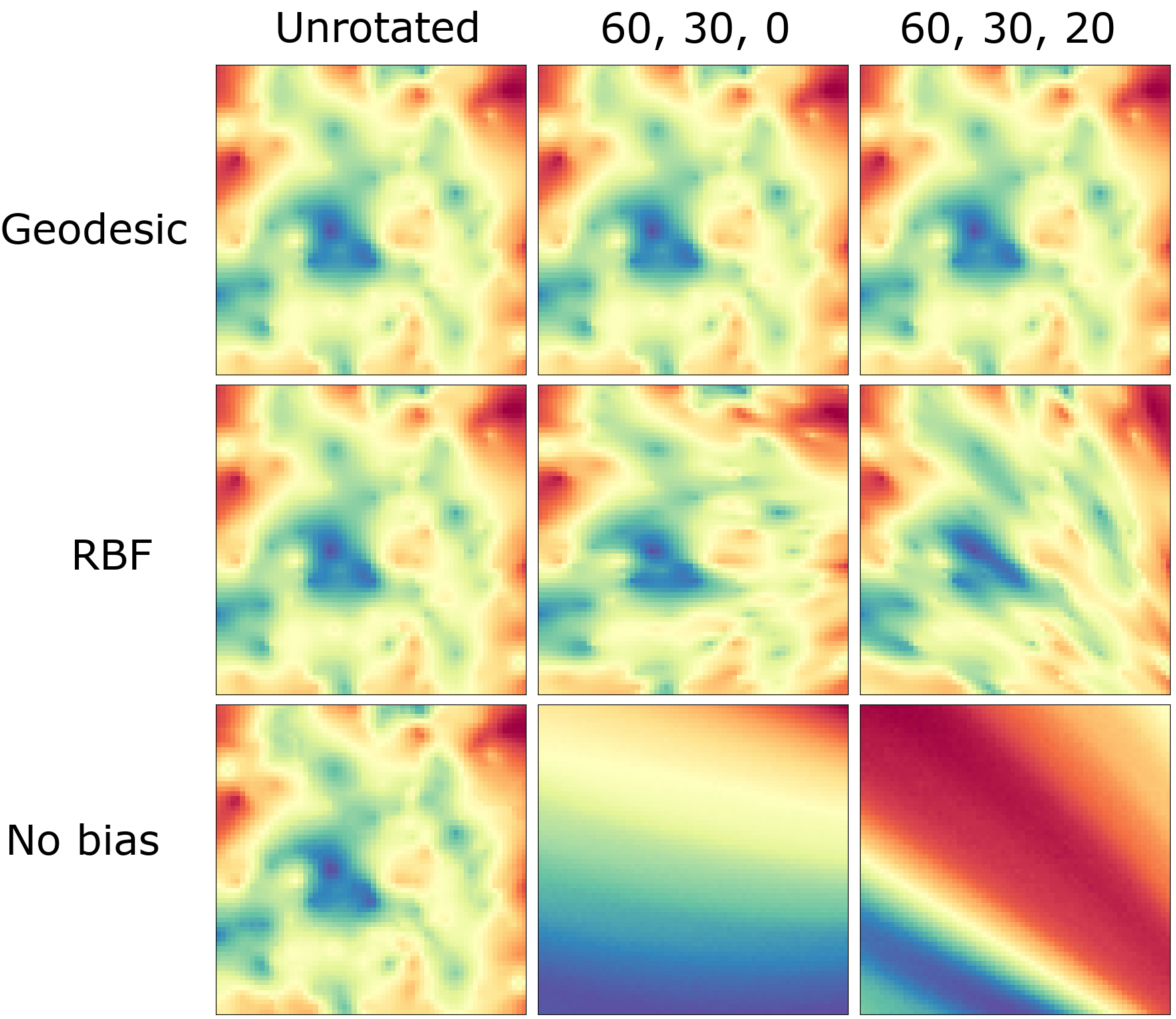
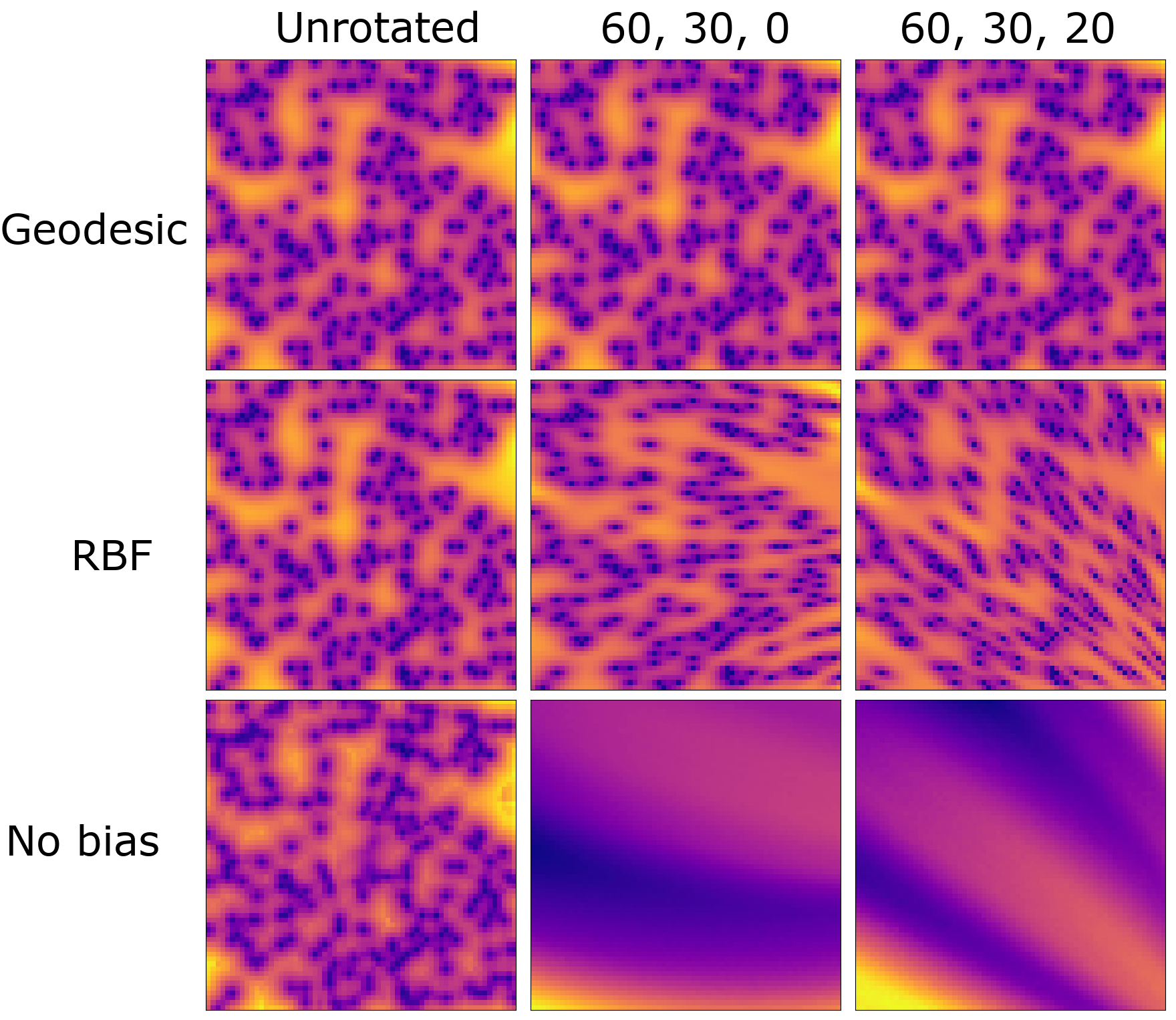
Figure 4: An example of mean and uncertainty predictions of the Geodesic, RBF, and Embed variants on the same sphere-stationary GP task. RBF’s are visibly distorted under sphere rotations, while Embed fails to give a meaningful prediction outside of the training range.

Susceptible-Infected-Recovered (SIR):

For the SIR benchmark, we simulate tasks from a SIR model. It is governed by an infection rate, $\beta$, a recovery rate, $\gamma$, and the number of initial infections, $\omega$. We sample $\beta\sim\operatorname{Beta}(2,8)$, $\gamma\sim\operatorname{InvGamma}(5,0.4)$, and $\omega\sim\operatorname{randint}(1,5)$. The infection rate, $\beta$, is decreased as an inverse function of distance from the infected individual. In expectation, this parameter setting corresponds to an infection rate of 20% upon exposure and a 10-day recovery period (similar to COVID-19). We roll out simulations for 25 steps and randomly sample steps to create tasks. We use a grid size of 64x64 on the domain $[-2,2]^{2}$. Similar to the 2D GP benchmark, we sample the number of contexts points uniformly from $[128,512]$, which corresponds to 3%-12.5% of pixels. We test on a separate 1024 points, corresponding to 25% of the points on a 64x64 grid. We train over 100K batches, each with batch size 8, and validate every 10K steps on 5K batches. We test on 5K unseen batches. We use the AdamW optimizer with $\beta_{1}=0.9$, $\beta_{2}=0.999$, and weight decay 1e-4. We clip maximum gradient norms at 0.5 and use a cosine learning rate schedule which starts at 1e-4 and decays to 1e-5.

ERA5

We largely follow the setup in [2] with ERA5 [11] surface air temperatures. To test learning over time and generalization across space, we train models on tasks from central Europe $[42^{\circ}\mathrm{N},\,53^{\circ}\mathrm{N}]\times[8^{\circ}\mathrm{W},\,28^{\circ}\mathrm{W}]$ and test them on tasks from northern Europe $[53^{\circ}\mathrm{N},\,63^{\circ}\mathrm{N}]\times[8^{\circ}\mathrm{W},\,28^{\circ}\mathrm{W}]$ and western Europe $[42^{\circ}\mathrm{N},\,53^{\circ}\mathrm{N}]\times[-4^{\circ}\mathrm{W},\,8^{\circ}\mathrm{W}]$ over random 30-hour segments of time. When testing on northern Europe, we use western Europe as a validation set and select the best model for testing and vice versa when testing on western Europe. Unlike [2] which inpaints several frames over time, we change the benchmark to forecast the weather in the next 6 hours. We also add “hour of day” to the feature set and increase the resolution from $0.5^{\circ}$ to $0.25^{\circ}$. The input data is all standardized based on the training set, i.e. central Europe. The task consists of 4 context frames and 1 test frame, each separated by 6 hours. The inputs we use are x=(elevation, hour of day), s=(latitude, longitude), t=time, f=surface temperature. Each task consists of a 30x30 image or $7.5^{\circ}\times 7.5^{\circ}$ at a resolution of $0.25^{\circ}$. We sample context points uniformly from 45 to 225 from each time step in the context set, corresponding to approximately 5% and 25% of the number of pixels. The test set for each task consists of all 900 pixels from the target time step. We train on 100K batches, each of size 8, and validate every 5K steps on 5K batches. We test on 5K batches from the test region. Following [2], we use the AdamW optimizer with $\beta_{1}=0.9$, $\beta_{2}=0.999$, and weight decay 1e-4. We clip maximum gradient norms at 0.5 and use a constant learning rate of 5.0e-4.

Bejing Multi-City Air Quality:

For this benchmark, we use the Beijing Multi-Site Air Quality benchmark from the UCI repository [8]. This dataset measures pollution across 12 cities in China and includes not only location and time, but also windspeed, wind direction, dewpoint, temperature, and rain. We include these as fixed covariates (x), as well as some generated ones including “day of week” and “is weekend.” Because this is a comparatively easy dataset, we train over only 10K batches, each of size 32. Most models overfit quickly, so we validate on 500 batches every 500 steps and use the model with the lowest validation score for testing. The data is split in temporal order into 80% train, 10% validation, and 10% test. All inputs are standardized based on the training split. The number of context points are fixed at 624, which represents the last 48 hours of data for all 12 locations plus a buffer of 12 to ensure that a random slice into the dataset doesn’t leave some locations without a full 48 hours. We test on 84 points, which corresponds to the next 6 hours for all 12 locations plus a buffer of 12 to ensure that all 12 locations are predicted hourly for a full 6 hours. These figures are not always precise, however, since there are a small number of gaps in the data, which means that not all tasks may contain exactly the 48-6 hour split.We test on 5K batches from the test region. We use the AdamW optimizer with $\beta_{1}=0.9$, $\beta_{2}=0.999$, and weight decay 1e-4. We clip maximum gradient norms at 0.5 and use a cosine learning rate schedule which starts at 1e-3 and decays to 1e-5.

Generic Spatial:

For this benchmark, we use the following generic spatial model written in Numpyro [30] to generate samples from the prior predictive distribution:

$$\begin{split}\ell&\sim\text{Beta}(\alpha,\beta)\\ \mathbf{f}\mid\ell&\sim\mathcal{GP}(\mu(\cdot),\mathcal{K}(\cdot,\cdot\mid\ell))\\ \bm{\eta}&=\mathbf{X}\bm{\gamma}+\mathbf{f}\\ \sigma^{2}&\sim\text{HalfNormal}(\nu)\\ \mathbf{y}\mid\bm{\eta},\sigma^{2}&\sim\text{Normal}(\bm{\eta},\sigma^{2})\end{split}$$ (5)

For each batch we sample 128 spatial locations, $\mathbf{s}\sim\text{Uniform}\left([-2,2]\right)$, and a 10-dimensional vector of fixed effects associated with each location, $\mathbf{X}\sim\mathcal{N}(0,1)\in\mathbb{R}^{128\times 10}$, and feed these through the Numpyro model to generate samples from the prior predictive. We sample between 13 and 64 context points, which corresponds to approximately 3% and 12.5% of the number of pixels on a 16x16 grid. We test on a separate 64 points. We use the AdamW optimizer with $\beta_{1}=0.9$, $\beta_{2}=0.999$, and weight decay 1.0e-4. We clip maximum gradient norms at 0.5 and use a cosine learning rate schedule which starts at 1e-3 and decays to 2e-5.

At test/inference time, we sample 5 tasks from the prior and compare TabPFN, TNP-D, PT-TE-TNP, BSA-TNP, and full MCMC with the NUTS sampler. When running MCMC with NUTS, we use 4 chains each with 2000 warmup steps and 2000 samples. The total “training time” recorded for NUTS MCMC is the collective time taken for all 5 tasks. Inference time for all deep learning models is less than a second, so we do not list it. According to [20], TabPFN was pretrained over two weeks on eight GPUs and does not (yet) provide the option to return log likelihoods.

This benchmark demonstrates that BSA-TNP can generate posterior predictives that are just as accurate as full MCMC with NUTS while requiring only half the time to train. Furthermore, once trained, inference can be conducted instantaneously, whereas MCMC requires another $\approx$ 20 minutes per task.

Table 8: Generic Spatial Modeling.

Model	NLL	MAE	RMSE	CVG at 95%	Train (min)
TabPFN	—	$1.20\pm 0.12$	$1.50\pm 0.13$	$0.97\pm 0.02$	—
TNP-D	$1.64\pm 0.15$	$0.98\pm 0.11$	$1.25\pm 0.14$	$0.92\pm 0.03$	$\mathbf{45.13\pm 0.63}$
PT-TE-TNP	$1.64\pm 0.13$	$0.96\pm 0.12$	$1.22\pm 0.13$	$\mathbf{0.94\pm 0.04}$	$123.94\pm 1.53$
BSA-TNP	$\mathbf{1.54\pm 0.17}$	$\mathbf{0.90\pm 0.13}$	$\mathbf{1.15\pm 0.15}$	$\mathbf{0.94\pm 0.04}$	$51.48\pm 0.93$
NUTS MCMC	$\mathbf{1.53\pm 0.18}$	$\mathbf{0.91\pm 0.13}$	$\mathbf{1.16\pm 0.15}$	$\mathbf{0.93\pm 0.03}$	$102.86\pm 0.00$

Appendix C Complexity and Estimated FLOPS

In Table 9, we provide complexity estimates for the primary models compared in this paper. In Table 10, we provide estimated training and inference GFLOPS for each model. These are estimated using JAX’s cost analysis on functions lowered to HLO and compiled. These figures change from benchmark to benchmark based on the batch size and distribution of test and context points. We provide estimates for 2D GPs since this was our most generic benchmark. Notably, while ConvCNP has the lowest estimated GFLOPS for training and inference, it doesn’t translate into wallclock speed, likely due to poorer high bandwidth memory (HBM) accesses and the large induced grid that must be encoded and decoded for every task.

Table 9: Time and space complexity. $n_{c}$ is the number of context points, $n_{t}$ is number of test points, $n_{i}$ is number of inducing points, and $n_{b}$ is block size.

Model	Time	Space
ConvCNP	$\mathcal{O}(n_{c}n_{i}+n_{i}n_{t})$	$\mathcal{O}(n_{c}n_{i}+n_{i}n_{t})$
TNP-D	$\mathcal{O}((n_{c}+n_{t})^{2})$	$\mathcal{O}((n_{c}+n_{t})^{2})$
PT-TE-TNP	$\mathcal{O}(k(n_{c}+n_{t}))$	$\mathcal{O}(k(n_{c}+n_{t}))$
BSA-TNP	$\mathcal{O}(n_{c}^{2}+n_{c}n_{t})$	$\mathcal{O}(n_{b}^{2})$

Table 10: GFLOPS estimates on 2D GP and wallclock times. GFLOPs are estimated using JAX’s cost analysis on functions lowered to HLO and then compiled for a device.

Model	Train GFLOPS	Infer GFLOPS	Train (min)	Infer (batch/s)
ConvCNP	$\mathbf{88}$	$\mathbf{23}$	$121.10\pm 1.02$	$27.56\pm 0.04$
TNP-D	$217$	$72$	$65.27\pm 0.04$	$63.95\pm 0.40$
PT-TE-TNP	$310$	$101$	$72.40\pm 0.08$	$73.35\pm 0.77$
BSA-TNP	$94$	$31$	$\mathbf{36.98\pm 0.09}$	$\mathbf{103.74\pm 0.43}$

Appendix D Convergence

To visualize how bias can accelerate convergence, we provide the validation NLL vs. iteration plot below from the SIR benchmark, which demonstrates that G-invariant bias permits almost immediate convergence to the optimal solution. Furthermore, this performance was maintained under shifting and scaling, unlike TNP-D.

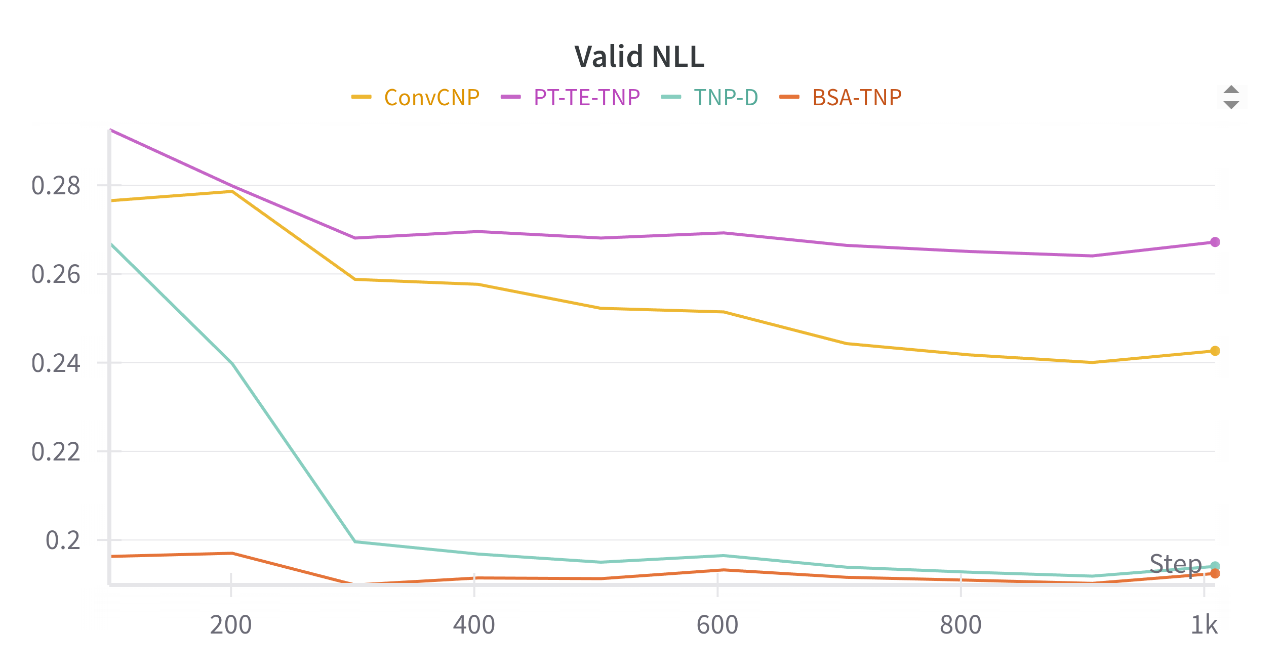
Figure 5: Validation NLL on the SIR benchmark for seed 91. All seeds exhibited the same pattern.

Appendix E Biased Scan Attention

This section details the fundamental operations involved in Biased Scan Attention (BSA). The only requirements of BSA, like its predecessors, are keeping track of the maximum attention score, $m(x)$, the normalization constant, $\ell(x)$, and the unnormalized output, $\mathbf{\tilde{O}}$. For every tile, $j$, Equation 6 is computed. Then for the first tile Equation 7 is computed, and for subsequent tiles, $j>1$, Equation 8 is computed.

$$\begin{split}x_{i}^{(j)}&=\mathbf{Q}^{(j)}_{e}\mathbf{K}^{(j)\intercal}_{e}/\sqrt{d_{e}}+\sum_{\omega\in\{x,s,t\}}\mathcal{K}_{\omega}(\mathbf{Q}_{\omega}^{(j)},\mathbf{K}_{\omega}^{(j)})\\ f(x)^{(j)}&=\left[e^{x_{1}^{(j)}-m(x)^{(j)}},\ldots,e^{x_{B}^{(j)}-m(x)^{(j)}}\right]\\ \end{split}$$ (6)

$$\begin{split}m(x)^{(1)}&=\operatorname{rowmax}(x^{(1)})\\ \ell(x)^{(1)}&=\operatorname{rowsum}(f(x)^{(1)})\\ \mathbf{\tilde{O}}^{(1)}&=f(x)^{(1)}\mathbf{V}^{(1)}\\ \end{split}$$ (7)

$$\begin{split}m(x)^{(j:j>1)}&=\max\left(m(x)^{(j-1)},\operatorname{rowmax}(x^{(j)})\right)\\ k^{(j:j>1)}&=e^{m(x)^{(j-1)}-m(x)^{(j)}}\\ \ell(x)^{(j:j>1)}&=k^{(j)}\ell(x)^{(j-1)}+\operatorname{rowsum}(f(x)^{(j)})\\ \mathbf{\tilde{O}}^{(j:j>1)}&=k^{(j)}\mathbf{\tilde{O}}^{(j-1)}+f(x)^{(j)}\mathbf{V}^{(j)}\\ \end{split}$$ (8)

In short, as each block of size $B$ is processed, three updates occur: (1) the maximum score, $m(x)^{(j)}$, is updated, (2) the normalization constants, $\ell(x)^{(j)}$, are rescaled and updated, and the (3) unnormalized output, $\mathbf{\tilde{O}}^{(j)}$, is rescaled and updated. In the final step, the output is normalized by the final row sums, $\mathbf{O}=\operatorname{diag}(\ell(x)^{(n)})^{-1}\mathbf{\tilde{O}}^{(n)}$.

Appendix F Multiresolution 2D GPs

The following visualizes a batch of multiresolution 2D GP tasks with predictions from BSA-TNP. By using a coarser resolution for the area surrounding the target region, the number of pixels is reduced by $\approx$ 78%.

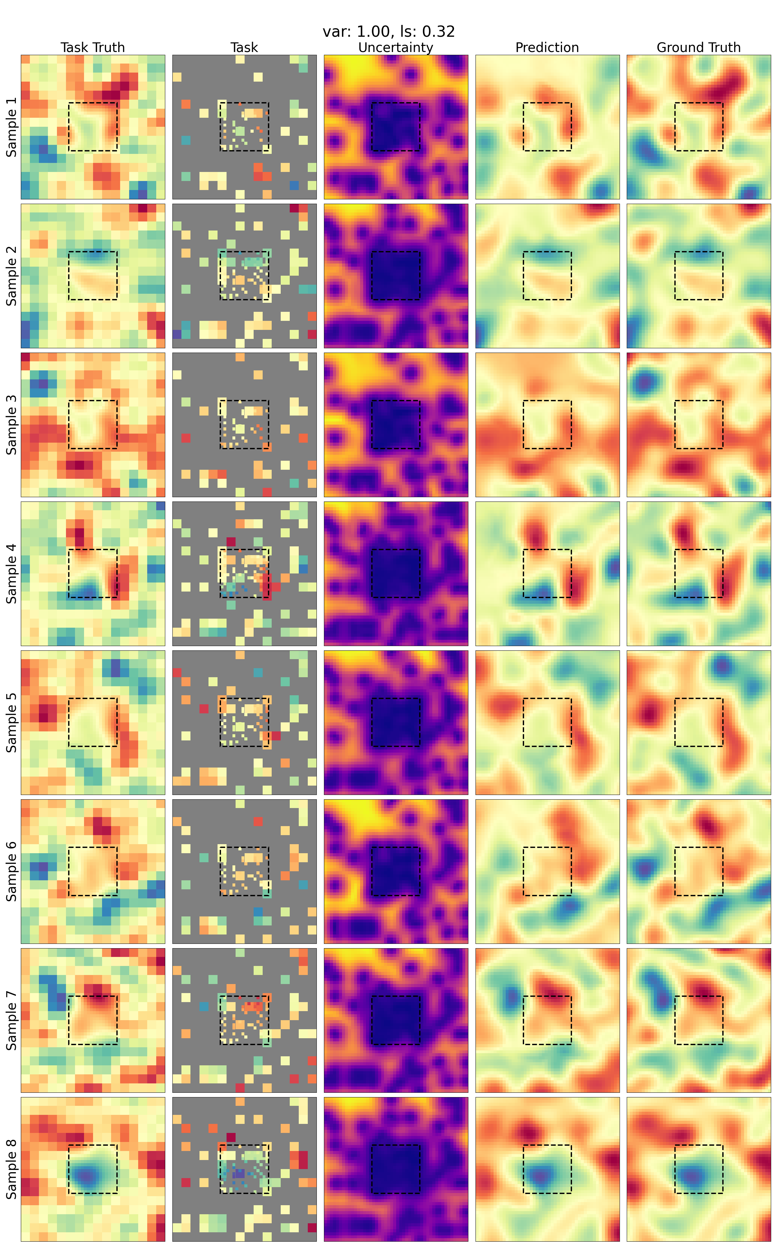
Figure 6: An example of a batch of multiresolution 2D GP tasks. Predictions are from BSA-TNP.

Appendix G Group Invariance Theory Proof

In this section we prove Theorem 1, using the same notations and definitions introduced in Section 3.

Proof.

We assume a probability space $(\Omega,\mathcal{F},\mathbb{P})$ with the stochastic process $F$ taking values in $Y=\mathbb{R}^{n}$ endowed with the Borel $\sigma$-algebra, so that regular conditional distributions exist. Let $\mu_{\mathbf{d}}$ denote the law of $F(\mathbf{d})$, and $\mu_{\mathbf{d}_{t}\mid\mathbf{d}_{c},\mathbf{f}_{c}}$ the conditional law of $F(\mathbf{d}_{t})\mid F(\mathbf{d}_{c})=\mathbf{f}_{c}$, that is the probability measures defined by $\mu_{\mathbf{d}}(A)=\mathbb{P}(F(\mathbf{d})\in A)$ and $\mu_{\mathbf{d}_{t}\mid\mathbf{d}_{c},\mathbf{f}_{c}}(A)=\mathbb{P}(F(\mathbf{d}_{t})\in A\mid F(\mathbf{d}_{c})=\mathbf{f}_{c})$. Details on the definitions of $\sigma$-algebras, measures, Lebesgue-Stieltjes integration, and conditional probabilities can be found e.g. in [25].

$\implies$: Assume $F$ is $G$-stationary, then for all measurable $A\subseteq Y^{|\mathbf{d}_{t}|}$ and $B\subseteq Y^{|\mathbf{d}_{c}|}$, by (1) consistency of regular conditional distributions, and (2) $G$-stationarity of $F$ so that $\mu_{\mathbf{d}}=\mu_{g\mathbin{\bm{\cdot}}\mathbf{d}}$, it follows that:

$$\int_{\mathbf{f}_{c}\in B}\mu_{\mathbf{d}_{t}\mid\mathbf{d}_{c},\mathbf{f}_{c}}(A)\,\mathrm{d}\mu_{\mathbf{d}_{c}}(\mathbf{f}_{c}) \stackrel{{\scriptstyle(1)}}{{=}}\mu_{(\mathbf{d}_{t},\mathbf{d}_{c})}(A\times B)$$

$$\stackrel{{\scriptstyle(2)}}{{=}}\mu_{g\mathbin{\bm{\cdot}}(\mathbf{d}_{t},\mathbf{d}_{c})}(A\times B)$$

$$\stackrel{{\scriptstyle(1)}}{{=}}\int_{\mathbf{f}_{c}\in B}\mu_{g\mathbin{\bm{\cdot}}\mathbf{d}_{t}\mid g\mathbin{\bm{\cdot}}\mathbf{d}_{c}\mathbf{f}_{c}}(A)\,\mathrm{d}\mu_{g\mathbin{\bm{\cdot}}\mathbf{d}_{c}}(\mathbf{f}_{c})$$

$$\stackrel{{\scriptstyle(2)}}{{=}}\int_{\mathbf{f}_{c}\in B}\mu_{g\mathbin{\bm{\cdot}}\mathbf{d}_{t}\mid g\mathbin{\bm{\cdot}}\mathbf{d}_{c}\mathbf{f}_{c}}(A)\,\mathrm{d}\mu_{\mathbf{d}_{c}}(\mathbf{f}_{c}).$$

This equality holds for any measurable $B$. By Lemma 1 we get that for all $A$, for $\mu_{\mathbf{d}_{c}}$-almost-every $\mathbf{f}_{c}$, $\mu_{g\mathbin{\bm{\cdot}}\mathbf{d}_{t}\mid g\mathbin{\bm{\cdot}}\mathbf{d}_{c},\mathbf{f}_{c}}(A)=\mu_{\mathbf{d}_{t}\mid\mathbf{d}_{c},\mathbf{f}_{c}}(A)$. Lemma 2 allows us to swap the quantifiers and get that for $\mu_{\mathbf{d}_{c}}$-almost-every $\mathbf{f}_{c}$ the laws $\mu_{g\mathbin{\bm{\cdot}}\mathbf{d}_{t}\mid g\mathbin{\bm{\cdot}}\mathbf{d}_{c},\mathbf{f}_{c}}$ and $\mu_{\mathbf{d}_{t}\mid\mathbf{d}_{c},\mathbf{f}_{c}}$ are equal. Conditional distributions are defined with respect to equality almost everywhere in the conditioning argument, therefore we may conclude that the distributions of $F(\mathbf{d}_{t})\mid F(\mathbf{d}_{c})=\mathbf{f}_{c}$ and $F(g\mathbin{\bm{\cdot}}\mathbf{d}_{t})\mid F(g\mathbin{\bm{\cdot}}\mathbf{d}_{c})=\mathbf{f}_{c}$ are equal, and thus, the posterior predictive map $\pi$ is G-invariant.

$\impliedby$: Assume the posterior predictive map $\pi$ is G-invariant. Let $\mathbf{d}_{c}$ and $\mathbf{f}_{c}$ be the empty set. We immediately get that

$$F(g\mathbin{\bm{\cdot}}\mathbf{d}_{t})=\pi(g\mathbin{\bm{\cdot}}\mathbf{d}_{c},\mathbf{f}_{c},g\mathbin{\bm{\cdot}}\mathbf{d}_{t})=\pi(\mathbf{d}_{c},\mathbf{f}_{c},\mathbf{d}_{t})=F(\mathbf{d}_{t})$$

and hence, F is G-invariant.

∎

Lemma 1.

If $\int_{E}f\,\mathrm{d}\mu=\int_{E}g\,\mathrm{d}\mu$ for all measurable sets $E$ and a non-negative measure $\mu$, then $f=g$ $\mu$-almost-everywhere.

Proof.

Consider the set $E_{n}=\{x:f(x)-g(x)\geq\frac{1}{n}\}$, which is measurable since $f,g$ are integrable. Then $0=\int_{E_{n}}(f-g)\,\mathrm{d}\mu\geq\frac{1}{n}\mu(E_{n})\geq 0$, so it must be that $\mu(E_{n})=0$. As a countable union of null sets, it must be that $\{x:f(x)-g(x)>0\}=\bigcup_{n=1}^{\infty}E_{n}$ is null. By a symmetric argument, it must be that $\{x:g(x)-f(x)>0\}$ is null. Therefore $f(x)=g(x)$ for $\mu$-almost-every $x$. ∎

Lemma 2.

Let $\mu$ be a probability measure over $\mathcal{B}(\mathbb{R}^{d})$ and $f,g:\mathcal{B}(\mathbb{R}^{k})\times\mathbb{R}^{d}\to[0,1]$ Markov kernels, that is functions, such that

1. for $\mu$-almost-every $x$, $f(\cdot,x),g(\cdot,x)$ are probability measures,

2. for all $A$, $f(A,\cdot),g(A,\cdot)$ are measurable functions.

If for all $A$, for $\mu$-almost-every $x$, $f(A,x)=g(A,x)$, then $f(\cdot,x)=g(\cdot,x)$ for $\mu$-almost-every $x$.

Proof.

First consider sets of the form $A=(a_{1},b_{1})\times\ldots\times(a_{k},b_{k})$ with $a_{i},b_{i}\in\mathbb{Q}$ for all $i=1,\ldots,k$, that is open rectangles in $\mathbb{R}^{k}$ with rational coordinates, and enumerate this countable family as $A_{n},n\in\mathbb{N}$. By assumption, $E_{n}=\{x:f(A_{n},x)\neq g(A_{n},x)\}$ and $F=\{x:f(\cdot,x),g(\cdot,x)\text{ are not probability measures}\}$ are null with respect to $\mu$, so $N:=\bigcup_{n\in\mathbb{N}}E_{n}\cup F$ is null.

Now for fixed $x\in\mathbb{R}^{d}\setminus N$, consider the set $\mathcal{E}=\{B\in\mathcal{B}(\mathbb{R}^{k}):f(B,x)=g(B,x)\}$. Since $f(\cdot,x),g(\cdot,x)$ are measures, $\mathcal{E}$ is a $\sigma$-algebra,. Moreover, by definition of $N$, $\mathcal{E}$ contains the set of all rational open rectangles in $\mathbb{R}^{k}$. Since these rectangles generate $\mathcal{B}(\mathbb{R}^{k})$, it must be that $\mathcal{B}(\mathbb{R}^{k})\subseteq\mathcal{E}$ and hence the measures $f(\cdot,x)$ and $g(\cdot,x)$ are equal. Since this holds for all $x\in\mathbb{R}^{k}\setminus N$, the proof is complete. ∎

Appendix H BSA-TNP G-Invariance Proof

In this section we prove Theorem 2, using the same notations, definitions and BSA-TNP architecture module names introduced in Sections 3, 4.

Proof.

This follows by tracing $(g\mathbin{\bm{\cdot}}\mathbf{d}_{c},g\mathbin{\bm{\cdot}}\mathbf{d}_{t})$ through the BSA-TNP architecture.

1. By the assumption of the theorem $\mathrm{Embed}_{\varphi}$ is $G$-invariant in $\mathbf{d}_{c},\mathbf{d}_{t}$.

2. The kernels used in the attention bias are $G$-invariant. As no other calculation within the attention mechanism involve $\mathbf{d}_{\{c,t\}}$, we get that $\mathrm{BSA}$ is G-invariant. Thus, $\mathrm{BSA}(\mathbf{qs},\mathbf{d}_{q},\mathbf{ks},\mathbf{d}_{k})=\mathrm{BSA}(\mathbf{qs},g\mathbin{\bm{\cdot}}\mathbf{d}_{q},\mathbf{ks},g\mathbin{\bm{\cdot}}\mathbf{d}_{k})$. Consequently, $\mathbf{e}_{c}^{\prime}=\mathrm{BSA}(\mathbf{e}_{c},g\mathbin{\bm{\cdot}}\mathbf{d}_{c},\mathbf{e}_{c},g\mathbin{\bm{\cdot}}\mathbf{d}_{c})=\mathrm{BSA}(\mathbf{e}_{c},\mathbf{d}_{c},\mathbf{e}_{c},\mathbf{d}_{c})$ and $\mathbf{e}_{t}^{\prime}=\mathrm{BSA}(\mathbf{e}_{t},g\mathbin{\bm{\cdot}}\mathbf{d}_{t},\mathbf{e}_{c},g\mathbin{\bm{\cdot}}\mathbf{d}_{c})=\mathrm{BSA}(\mathbf{e}_{t},\mathbf{d}_{t},\mathbf{e}_{c},\mathbf{d}_{c})$. As a result, the KRBlock’s output $\mathbf{e}^{\prime}_{\{c,t\}}$ is $G$-invariant with respect to $\mathbf{d}_{c},\mathbf{d}_{t}$.

3. The projection head only takes the encoding $\mathbf{e}^{\prime}_{t}$ output by the final KRBlock, and thus agnostic to $\mathbf{d}_{c},\mathbf{d}_{t}$.

By the above, BSA-TNP consists only of G-invariant operations: $\mathrm{Embed}_{\varphi}$, followed by an arbitrary number of KRBlocks, and the projection head, and therefore stacking these operations results in a $G$-invariant model in $\mathbf{d}_{c},\mathbf{d}_{t}$. ∎

References

- (1) Tom R. Andersson, Wessel P. Bruinsma, Stratis Markou, James Requeima, Alejandro Coca-Castro, Anna Vaughan, Anna-Louise Ellis, Matthew A. Lazzara, Dani Jones, Scott Hosking, and et al. Environmental sensor placement with convolutional gaussian neural processes. Environmental Data Science, 2:e32, 2023.
- (2) Matthew Ashman, Cristiana Diaconu, Junhyuck Kim, Lakee Sivaraya, Stratis Markou, James Requeima, Wessel P Bruinsma, and Richard E. Turner. Translation equivariant transformer neural processes. In Ruslan Salakhutdinov, Zico Kolter, Katherine Heller, Adrian Weller, Nuria Oliver, Jonathan Scarlett, and Felix Berkenkamp, editors, Proceedings of the 41st International Conference on Machine Learning, volume 235 of Proceedings of Machine Learning Research, pages 1924–1944. PMLR, 21–27 Jul 2024.
- (3) Matthew Ashman, Cristiana Diaconu, Eric Langezaal, Adrian Weller, and Richard E. Turner. Gridded transformer neural processes for large unstructured spatio-temporal data, 2024.
- (4) Mahmoud Assran, Quentin Duval, Ishan Misra, Piotr Bojanowski, Pascal Vincent, Michael Rabbat, Yann LeCun, and Nicolas Ballas. Self-supervised learning from images with a joint-embedding predictive architecture. In Proceedings of the IEEE/CVF Conference on Computer Vision and Pattern Recognition (CVPR), 2023.
- (5) Iz Beltagy, Matthew E. Peters, and Arman Cohan. Longformer: The long-document transformer. arXiv:2004.05150, 2020.
- (6) Srinadh Bhojanapalli, Ayan Chakrabarti, Andreas Veit, Michal Lukasik, Himanshu Jain, Frederick Liu, Yin-Wen Chang, and Sanjiv Kumar. Leveraging redundancy in attention with reuse transformers, 2022.
- (7) James Bradbury, Roy Frostig, Peter Hawkins, Matthew James Johnson, Chris Leary, Dougal Maclaurin, George Necula, Adam Paszke, Jake VanderPlas, Skye Wanderman-Milne, and Qiao Zhang. JAX: composable transformations of Python+NumPy programs, 2018.
- (8) Song Chen. Beijing Multi-Site Air Quality [dataset]. UCI Machine Learning Repository, 2017.
- (9) Rewon Child, Scott Gray, Alec Radford, and Ilya Sutskever. Generating long sequences with sparse transformers, 2019.
- (10) Krzysztof Marcin Choromanski, Valerii Likhosherstov, David Dohan, Xingyou Song, Andreea Gane, Tamas Sarlos, Peter Hawkins, Jared Quincy Davis, Afroz Mohiuddin, Lukasz Kaiser, David Benjamin Belanger, Lucy J Colwell, and Adrian Weller. Rethinking attention with performers. In International Conference on Learning Representations, 2021.
- (11) Copernicus Climate Change Service. Near surface meteorological variables from 1979 to 2018 derived from bias-corrected reanalysis, 2020. Dataset.
- (12) Tri Dao. FlashAttention-2: Faster attention with better parallelism and work partitioning. In International Conference on Learning Representations (ICLR), 2024.
- (13) Tri Dao, Daniel Y. Fu, Stefano Ermon, Atri Rudra, and Christopher Ré. FlashAttention: Fast and memory-efficient exact attention with IO-awareness. In Advances in Neural Information Processing Systems (NeurIPS), 2022.
- (14) Juechu Dong, Boyuan Feng, Driss Guessous, Yanbo Liang, and Horace He. Flex attention: A programming model for generating optimized attention kernels, 2024.
- (15) Leo Feng, Hossein Hajimirsadeghi, Yoshua Bengio, and Mohamed Osama Ahmed. Latent bottlenecked attentive neural processes. In The Eleventh International Conference on Learning Representations, 2023.
- (16) Leo Feng, Frederick Tung, Hossein Hajimirsadeghi, Yoshua Bengio, and Mohamed Osama Ahmed. Memory efficient neural processes via constant memory attention block, 2024.
- (17) Marta Garnelo, Dan Rosenbaum, Christopher Maddison, Tiago Ramalho, David Saxton, Murray Shanahan, Yee Whye Teh, Danilo Rezende, and S. M. Ali Eslami. Conditional neural processes. In Jennifer Dy and Andreas Krause, editors, Proceedings of the 35th International Conference on Machine Learning, volume 80 of Proceedings of Machine Learning Research, pages 1704–1713. PMLR, 10–15 Jul 2018.
- (18) Marta Garnelo, Jonathan Schwarz, Dan Rosenbaum, Fabio Viola, Danilo J. Rezende, S. M. Ali Eslami, and Yee Whye Teh. Neural processes, 2018.
- (19) Jonathan Gordon, Wessel P. Bruinsma, Andrew Y. K. Foong, James Requeima, Yann Dubois, and Richard E. Turner. Convolutional conditional neural processes. In International Conference on Learning Representations, 2020.
- (20) Noah Hollmann, Samuel Müller, Lennart Purucker, Arjun Krishnakumar, Max Körfer, Shi Bin Hoo, Robin Tibor Schirrmeister, and Frank Hutter. Accurate predictions on small data with a tabular foundation model. 637(8045):319–326. Publisher: Nature Publishing Group.
- (21) Junfeng Hu, Yuxuan Liang, Zhencheng Fan, Hongyang Chen, Yu Zheng, and Roger Zimmermann. Graph neural processes for spatio-temporal extrapolation. In Proceedings of the 29th ACM SIGKDD Conference on Knowledge Discovery and Data Mining, KDD ’23, page 752–763. ACM, August 2023.
- (22) Andrew Jaegle, Felix Gimeno, Andy Brock, Oriol Vinyals, Andrew Zisserman, and Joao Carreira. Perceiver: General perception with iterative attention. In Marina Meila and Tong Zhang, editors, Proceedings of the 38th International Conference on Machine Learning, volume 139 of Proceedings of Machine Learning Research, pages 4651–4664. PMLR, 18–24 Jul 2021.
- (23) Atharv Jain, Seiji Shaw, and Nicholas Roy. Learning attentive neural processes for planning with pushing actions, 2025.
- (24) Nikita Kitaev, Lukasz Kaiser, and Anselm Levskaya. Reformer: The efficient transformer. In International Conference on Learning Representations, 2020.
- (25) Achim Klenke. Probability Theory: A Comprehensive Course. Universitext. Springer Nature, third edition edition, 2020.
- (26) Juho Lee, Yoonho Lee, Jungtaek Kim, Adam Kosiorek, Seungjin Choi, and Yee Whye Teh. Set transformer: A framework for attention-based permutation-invariant neural networks. In Proceedings of the 36th International Conference on Machine Learning, pages 3744–3753, 2019.
- (27) Guiye Li and Guofeng Cao. Neural process for uncertainty-aware geospatial modeling. In Proceedings of the 7th ACM SIGSPATIAL International Workshop on AI for Geographic Knowledge Discovery, GeoAI ’24, pages 106–109. Association for Computing Machinery, 2024.
- (28) E. A. Nadaraya. On estimating regression. Theory of Probability & Its Applications, 9(1):141–142, 1964.
- (29) Tung Nguyen and Aditya Grover. Transformer neural processes: Uncertainty-aware meta learning via sequence modeling. arXiv preprint arXiv:2207.04179, 2022.
- (30) Du Phan, Neeraj Pradhan, and Martin Jankowiak. Composable effects for flexible and accelerated probabilistic programming in numpyro. arXiv preprint arXiv:1912.11554, 2019.
- (31) Ofir Press, Noah Smith, and Mike Lewis. Train short, test long: Attention with linear biases enables input length extrapolation. In International Conference on Learning Representations, 2022.
- (32) Markus N. Rabe and Charles Staats. Self-attention does not need memory, 2022.
- (33) Jay Shah, Ganesh Bikshandi, Ying Zhang, Vijay Thakkar, Pradeep Ramani, and Tri Dao. Flashattention-3: Fast and accurate attention with asynchrony and low-precision. In The Thirty-eighth Annual Conference on Neural Information Processing Systems, 2024.
- (34) Zhuoran Shen, Mingyuan Zhang, Haiyu Zhao, Shuai Yi, and Hongsheng Li. Efficient attention: Attention with linear complexities. In Proceedings of the IEEE/CVF Winter Conference on Applications of Computer Vision (WACV), pages 3531–3539, 2021.
- (35) Yi Tay, Dara Bahri, Liu Yang, Donald Metzler, and Da-Cheng Juan. Sparse sinkhorn attention, 2020.
- (36) Waldo R Tobler. A computer movie simulating urban growth in the detroit region. Economic geography, 46(sup1):234–240, 1970.
- (37) Ashish Vaswani, Noam Shazeer, Niki Parmar, Jakob Uszkoreit, Llion Jones, Aidan N Gomez, Ł ukasz Kaiser, and Illia Polosukhin. Attention is all you need. In I. Guyon, U. Von Luxburg, S. Bengio, H. Wallach, R. Fergus, S. Vishwanathan, and R. Garnett, editors, Advances in Neural Information Processing Systems, volume 30. Curran Associates, Inc., 2017.
- (38) A. Vaughan, W. Tebbutt, J. S. Hosking, and R. E. Turner. Convolutional conditional neural processes for local climate downscaling. Geoscientific Model Development, 15(1):251–268, 2022.
- (39) Anna Vaughan, Stratis Markou, Will Tebbutt, James Requeima, Wessel P. Bruinsma, Tom R. Andersson, Michael Herzog, Nicholas D. Lane, Matthew Chantry, J. Scott Hosking, and Richard E. Turner. Aardvark weather: end-to-end data-driven weather forecasting, 2024.
- (40) Sinong Wang, Belinda Z. Li, Madian Khabsa, Han Fang, and Hao Ma. Linformer: Self-attention with linear complexity, 2020.
- (41) Chengxuan Ying, Tianle Cai, Shengjie Luo, Shuxin Zheng, Guolin Ke, Di He, Yanming Shen, and Tie-Yan Liu. Do transformers really perform badly for graph representation? In Thirty-Fifth Conference on Neural Information Processing Systems, 2021.
- (42) Chengxuan Ying, Guolin Ke, Di He, and Tie-Yan Liu. Lazyformer: Self attention with lazy update, 2021.
- (43) Manzil Zaheer, Guru Guruganesh, Kumar Avinava Dubey, Joshua Ainslie, Chris Alberti, Santiago Ontanon, Philip Pham, Anirudh Ravula, Qifan Wang, Li Yang, et al. Big bird: Transformers for longer sequences. Advances in Neural Information Processing Systems, 33, 2020.