State-preparation and measurement error mitigation with non-computational states

Abstract

Error mitigation has enabled quantum computing applications with over one hundred qubits and deep circuits. The most general error mitigation methods rely on a faithful characterization of the noise channels of the hardware. However, fundamental limitations lead to unlearnable degrees of freedom of the underlying noise models when considering qubits. Here, we show how to leverage non-computational states as an additional resource to learn state-preparation errors in superconducting qubits. This allows one to fully constrain the noise models. We can thus independently and accurately mitigate state-preparation errors, gate errors and measurement errors. Our proposed method is also applicable to dynamic circuits with mid-circuit measurements. This work opens the door to improved error mitigation for measurements, both at the end of the circuit and mid-circuit.

I Introduction

Progress in quantum computing hardware and error mitigation has enabled utility-scale experiments Kim et al. (2023); Fischer et al. (2024); Fuller et al. (2025). At this scale, a brute-force classical simulation of the underlying quantum circuits is no longer possible. Moving forward, error mitigation may enable a quantum advantage before the onset of full fault-tolerance Zimborás et al. (2025). In the fault-tolerant regime error mitigation will remain relevant by enhancing performance and reducing residual logical errors beyond the capabilities of error correction alone Piveteau et al. (2021); Aharonov et al. (2025). Importantly, quantum computing is not only made of sequences of unitary gates. Mid-circuit measurements (MCMs) offer a powerful computational extension. They form the bedrock of dynamic circuits and enable entanglement distribution Bäumer et al. (2024a), improved algorithmic execution Córcoles et al. (2021); Bäumer et al. (2024b, 2025), and circuit cutting Piveteau and Sutter (2023); Brenner et al. (2023); Carrera Vazquez et al. (2024); Mitarai and Fujii (2021); Singh et al. (2024).

Many error mitigation methods rely on accurate noise learning experiments which also help characterize quantum processors at scale Van Den Berg et al. (2023); McKay et al. (2023); Kim et al. (2023). Gate noise is commonly characterized by repeating a gate layer to amplify its noise, e.g., in cycle benchmarking Erhard et al. (2019). A common assumption is to express the gate noise models as Pauli channels, which is in practice justified by applying Pauli twirling or randomized compiling Bennett et al. (1996); Knill (2004); Wallman and Emerson (2016). Pauli noise learning is made scalable by sparsifying the noise generators Van Den Berg et al. (2023). This is typically done by dropping the noise generators that do not match with the physical qubit couplings. In this framework, state-preparation and final measurement (SPAM) errors can be characterized with a model-free twirled readout circuit in a technique popularized as twirled readout error extinction (TREX) van den Berg et al. (2022). The SPAM errors on expectation value estimators are then mitigated in post-processing. By contrast, learning the noise models of MCMs requires extending cycle benchmarking Hines and Proctor (2025); Zhang et al. (2025). Here, readout-induced leakage can be characterized Hazra et al. (2025) and probabilistic error cancellation has been generalized to dynamic circuits Gupta et al. (2024); Koh et al. (2025); Hashim et al. (2025). Crucially, when separating SPAM errors from gate errors there are fundamentally non-learnable degrees of freedom. These degrees of freedom in the noise model are rigorously understood as the cut space of a cycle graph Chen et al. (2023a). The same happens when separating state from measurement errors. These non-learnable degrees of freedom can be circumvented by imposing symmetry assumptions on the noise models Van Den Berg et al. (2023) which may be violated in real experiments, or with ancilla qubits and ideal CNOT gates, implemented with error mitigation Yu and Wei (2025). For successful noise-model based error mitigation it can be crucial to go beyond these naive symmetry assumptions Fischer et al. (2024).

Recent work thus focuses on producing self-consistent noise characterization protocols that learn gate, state-preparation, and measurements noise. This approach results in a holistic noise model up to unlearnable gauge degrees of freedom such that any measured observable in circuits composed of the given state-preparation, gate, and measurement layers are insensitive to the gauge Chen et al. (2024). While this approach is sufficient for noise-learning based error mitigation of unitary circuits Chen et al. (2025a), it does not reveal the ground truth for all parameters of the noise model, such as state-preparation errors. This can limit certain uses of the noise model, such as combining noise models of different layers to form models for gate structures that have not been learned. Furthermore, its applicability to dynamic circuits with measurements and classical feed-forward still needs to be investigated.

Here, we show how non-computational states help learn state-preparation errors and establish a ground truth for a noise model of mid-circuit measurements. By using non-computational states, we can overcome the existing no-go theorems for noise learning Chen et al. (2023a, 2024). We demonstrate this in superconducting qubit hardware Krantz et al. (2019), but the method is applicable to other hardware platforms.

In Sec. II, we start by demonstrating the importance of characterizing state-preparation errors separately from measurement errors. In Sec. III, we propose a protocol to fix a ground truth in the noise model of MCMs. Finally, in Sec. IV we present numerical results of the proposed protocol. We discuss and conclude our work in Sec. V.

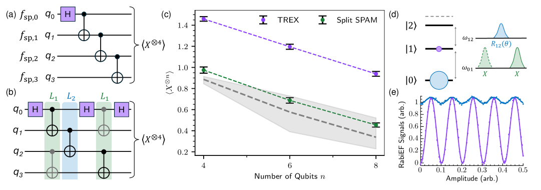
Figure 1: Splitting SPAM errors with non-computational states. (a) GHZ state preparation circuit. (b) A circuit inspired from (a) but with two unique CNOT layers $L_{1}$ and $L_{2}$ to facilitate gate noise learning. (c) SPAM error mitigation on the circuit in (b) with TREX (purple data) and a split mitigation of SPAM errors (green data). The error bars, discussed in Appendix B, represent $\pm 2\sigma$. The shaded area represents possible values of $\langle X^{\otimes n}\rangle$ based on the CNOT noise model, see Appendix C. The gray dashed line represents a symmetric splitting of the conjugate pairs of fidelities in the learned CNOT noise. (d) The first three levels of a superconducting transmon and the RabiEF pulse sequence. The circles indicate a thermal state, with populations corresponding to their sizes. (e) A RabiEF experiment on IBM Quantum hardware. The markers are hardware measurements and the curves are fits of $a\sin^{2}(b\theta)+c$ to the data. Here, $\theta$ is proportional to the pulse amplitude on the x-axis. Blue and purple are for the no-pi ($\cancel{\pi}$) and pi ($\pi$) RabiEF signals, respectively.

II Motivation

We now present an experiment, done on an IBM quantum Eagle device, showing that jointly mitigating state-preparation errors and measurement errors fails to error mitigate global observables of up to eight qubits. A GHZ state preparation circuit with a ladder structure of CNOT gates, shown in Fig. 1(a), turns the single-qubit $Z_{0}$ operator into a global $X^{\otimes n}$ operator. Hence, this $+1$ stabilizer is subject to measurement errors from all qubits, while only being affected by state-preparation errors from the first qubit. This makes the observable $O=X^{\otimes n}$ maximally sensitive to the separation of SPAM errors. We would thus like to study the circuit of Fig. 1(a). However, to account for gate noise we would need to learn the noise of the $n-1$ distinct layers of CNOT gates Van Den Berg et al. (2023); McKay et al. (2023). To reduce this overhead we convert the circuit in Fig. 1(a) to a similar circuit built from only two distinct layers of CNOT gates, see Fig. 1(b), which features the same behavior for the $X^{\otimes n}$ observable.

We mitigate the circuit in Fig. 1(b) with TREX van den Berg et al. (2022) by first measuring the raw expectation value $\langle O\rangle_{\text{raw}}$. All two-qubit gates are Pauli twirled so that the effective CNOT noise is a Pauli noise channel. We repeat this for $16n^{2}$ twirling configurations and collect $128$ shots per configuration.

Next, we correct SPAM errors in $\langle O\rangle_{\text{raw}}$ with TREX by normalizing it by a correction factor $\langle Z^{\star}\rangle$. This factor is found by measuring $Z^{\otimes{}n}$ on the all-zero initial state, with measurements twirled with $X$ gates and an assumed ideal prepared state. Under ideal state preparation the TREX correction factor is $\langle Z^{\star}\rangle=\prod_{i=0}^{n-1}f_{\text{m},i}$, where $f_{\text{m},i}$ denotes the final measurement fidelity and subscript $i$ denotes the corresponding qubit. However, in the presence of state-preparation errors the measured TREX mitigator becomes $\langle Z^{\star}\rangle=\prod_{i=0}^{n-1}f_{\text{sp},i}f_{\text{m},i}$, where $f_{\text{sp},i}$ are the state-preparation fidelities. Normalizing $\langle O\rangle_{\text{raw}}$ by $\langle Z^{\star}\rangle$ can thus cause TREX to overcompensate when the set of qubits whose state-preparation errors affect the observable (in our case only qubit 0) differs from the support of the observable (in our case all qubits), see, for example, Refs. Carrera Vazquez et al. (2024); Chen et al. (2025a).

Here, we measure $\langle Z^{\star}\rangle$ after a passive reset into the thermal state with $5000$ shots per each of the $16$ randomizations. We observe that TREX indeed over-corrects the expectation value $\langle X^{\otimes n}\rangle$ which we attribute to the factor $\prod_{i\neq 0}f_{\text{sp},i}\neq 1$, see the purple curve in Fig. 1(e). For our circuits with four and six qubits this even results in unphysical expectation values. This calls for a SPAM error mitigation that accounts for state-preparation errors independently of measurement errors.

III Noise learning with excited states

Jointly mitigating SPAM errors can lead to non-physical expectation values. We now demonstrate how to leverage non-computational states to separate state-preparation from measurement errors. Our work is based around the idea that well-controlled initial states, such as thermal states, can serve as a resource to this end.

III.1 Thermal states and passive reset

Learning the state-preparation error precisely necessitates stable state preparation in the computational basis. Therefore, we employ a simple passive reset by waiting more than $5-10\times T_{1}$ when initializing qubits. This results in a thermal state with a population following a Boltzmann distribution Ristè et al. (2012). Therefore, the probability to find the transmon in the excited state is $p_{\text{sp}}=\exp(-\hbar\omega_{01}/k_{B}T_{\text{eff}})$. Here, $\omega_{01}$ is the energy difference between the first excited state and the ground state, see Fig. 1(c). The effective temperatures of superconducting qubits $T_{\text{eff}}$ are typically above the $15~{\rm mK}$ temperature of dilution refrigerators. Furthermore, the population of the second excited state $\ket{2}$ is often negligible Jin et al. (2015), see also Appendix A.1. After a passive reset the qubit is thus in the thermal state $\rho_{\text{th}}=(1-p_{\text{sp}})\ket{0}\!\!\bra{0}+p_{\text{sp}}\ket{1}\!\!\bra{1}$ with typical $p_{\text{sp}}$ values in the $1-10\%$ range. Crucially, $p_{\text{sp}}$ can be precisely measured by driving an oscillation in the $\ket{1}\leftrightarrow\ket{2}$ subspace with the $R_{12}(\theta)$ gate and comparing it to a reference oscillation Geerlings et al. (2013); Jin et al. (2015), see Fig. 1(d). The probability $p_{\text{sp}}$ is estimated from the amplitudes of the no-pi ($\cancel{\pi}$) signal and the reference, or pi ($\pi$), signal, see Appendix A. This procedure, also known as a RabiEF experiment , provides a direct measurement of the state-preparation error $p_{\text{sp}}$ of a passive reset. Through the comparison to a reference oscillation, which is equally affected by measurement errors, the RabiEF experiment is mostly insensitive to measurement noise, see Appendix A.2. We can thus place ourselves in a situation where the state-preparation error is well known and measurable with sufficient accuracy by passively resetting the qubit.

III.2 Split mitigation of state and measurement errors

We can leverage our knowledge of state-preparation errors to prevent the TREX over-corrections shown in Sec. II. First, we measure the fidelities $f_{\text{sp},i}=1-2p_{\text{sp},i}$ of each qubit with RabiEF following a $10~{\rm ms}$ passive reset. Next, we multiply the correction factor $\langle Z^{\star}\rangle$ by the product $\prod_{i=1}^{n-1}f_{\text{sp},i}$ to obtain the mitigated expectation value

$$\langle O\rangle_{\text{mit}}=\frac{\langle O\rangle_{\text{raw}}\prod_{i=1}^{n-1}f_{\text{sp},i}}{\langle Z^{\star}\rangle}.$$ (1)

Crucially, the circuits to compute $\langle Z^{\star}\rangle$ must use the same passive reset as RabiEF so that the state-preparation error is consistent across all experiments. This results in physical expectation values, see the green curve in Fig. 1(e). Furthermore, these values are consistent with the noise levels of the CNOT gates. We learn their noise model and compute their impact on the expectation value of $X^{\otimes{}n}$ via a Clifford simulation, details are in Appendix C. Since we can only learn the CNOT noise up to the unlearnable degrees of freedom, we compute upper and lower bounds for the ideal observable with only CNOT noise, represented as the shaded area in Fig. 1(e), assuming physical noise channels. This area represents the possible range for $\langle O\rangle_{\text{raw}}$ after removing SPAM errors, and therefore $\langle O\rangle_{\text{mit}}$ falling within this area indicates success. The two experiments with six and eight qubits fall well within this area. The experiment with four qubits does not. Out-of-model errors, such as non-Markovian noise and noise generators with a weight greater than two, may cause this Govia et al. (2025).

III.3 Noise model of the measurement

We now develop a framework to completely specify the noise model of (mid-circuit) measurements built from the following assumptions. (i) State-preparation errors are bit flips. (ii) Noise occurs before measurements by convention, without loss of generality, see Fig. 2. (iii) After twirling, measurement errors are bit flips, i.e., Pauli strings containing only $I$’s or $X$’s. We twirl measurements following Ref. Beale and Wallman (2023). This diagonalizes the measurements and permutes the outcomes, while ensuring the post-measurement state is unchanged, see Fig. 3 of Ref. Beale and Wallman (2023).

With these assumptions, the Pauli Transfer Matrices (PTM), introduced in Appendix D, of the measurement noise channels will only contain non-zero diagonal elements in the entries corresponding to Pauli strings containing only $I$’s and $Z$’s. Therefore, whenever we now write the PTM of such a noise channel we omit rows and columns containing $X$’s or $Y$’s. Furthermore, we model the classical bit (cbit) as if it were a qubit living in a corresponding Hilbert space with the convention

$$\text{qubit}\otimes\text{cbit}.$$ (2)

For example, a bit-flip error on the qubit is denoted by $XI$ and a bit flip on the classical bit is $IX$. The entries of any PTM will always appear in lexicographic order, e.g., $II$, $IZ$, $ZI$, $ZZ$. To construct the PTM, we represent a measurement as a CNOT gate targeting the classical bit controlled by the qubit, and a subsequent measurement on the qubit; see Fig. 2. The model of the noisy measurement is built using the principle of deferred measurement Nielsen and Chuang (2000).

Our measurement noise model includes three possible error channels. (i) A state error, modeled as a bit flip on the qubit only, with probability $p_{\text{s}}$ and noise channel $\Lambda_{\text{s}}(\rho)=(1-p_{\text{s}})\rho+p_{\text{s}}XI\rho XI$. The PTM of $\Lambda_{\text{s}}$ is

$$\Gamma_{\text{s}}=\begin{pmatrix}1&0\\ 0&1-2p_{\text{s}}\\ \end{pmatrix}\otimes I.$$ (3)

This may correspond to a qubit decay at the end of the readout through a $T_{1}$ event. With twirling, this becomes an $X$ error instead of an amplitude damping channel. (ii) An assignment error, modeled as a bit flip on the classical bit only, with probability $p_{\text{a}}$ and noise channel $\Lambda_{\text{a}}(\rho)=(1-p_{\text{a}})\rho+p_{\text{a}}IX\rho IX$. The PTM of $\Lambda_{a}$ is

$$\Gamma_{\text{a}}=I\otimes\begin{pmatrix}1&0\\ 0&1-2p_{\text{a}}\\ \end{pmatrix}.$$ (4)

This may correspond to the readout misclassifying the state without a quantum error occurring on the qubit. Finally, (iii) a correlated error is a bit flip on both the classical and quantum bits with probability $p_{\text{c}}$ and noise channel $\Lambda_{\text{c}}(\rho)=(1-p_{\text{c}})\rho+p_{\text{c}}XX\rho XX$. The PTM of $\Lambda_{\text{c}}$ is

$$\Gamma_{\text{c}}=\begin{pmatrix}1&0&0&0\\ 0&1-2p_{\text{c}}&0&0\\ 0&0&1-2p_{\text{c}}&0\\ 0&0&0&1\\ \end{pmatrix}.$$ (5)

For example, this corresponds to a post-measurement $X$ error on the qubit, which is equivalent to the correlated error $\Lambda_{\text{c}}$ by propagating the $X$ back through the measurement.

The PTM $\Gamma_{\text{m}}$ of the noise model is obtained by multiplying the PTMs of the three error channels and the PTM of the ideal CNOT between the classical and quantum bit such that

$$\Gamma_{\text{m}}=\Gamma_{\text{CX}}\Gamma_{s}\Gamma_{a}\Gamma_{c}=\begin{pmatrix}1&0&0&0\\ 0&0&0&f_{\text{a}}f_{\text{s}}\\ 0&0&f_{\text{c}}f_{\text{s}}&0\\ 0&f_{\text{c}}f_{\text{a}}&0&0\\ \end{pmatrix}.$$ (6)

For readability we write the error fidelities $f_{\text{x}}\coloneqq(1-2p_{\text{x}})$ instead of their probabilities $p_{\text{x}}$. To learn the elements of $\Gamma_{\text{m}}$, we repeat the measurement $2k$ times in a cycle benchmarking experiment Zhang et al. (2025); Hines and Proctor (2025), resulting in

$$\Gamma_{\text{m}}^{2k}=\begin{pmatrix}1&0&0&0\\ 0&f_{\text{a}}^{2k}(f_{\text{c}}f_{\text{s}})^{k}&0&0\\ 0&0&(f_{\text{c}}f_{\text{s}})^{2k}&0\\ 0&0&0&f_{\text{a}}^{2k}(f_{\text{c}}f_{\text{s}})^{k}\\ \end{pmatrix}.$$ (7)

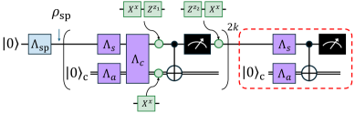
Figure 2: Measurement noise model. The qubit and the classical bit are indicated by the single and double lines, respectively. Cycle benchmarking learns the noise model, shown in purple, by repeating the measurement $2k$ times. The twirling gates are indicated in green; the binary variables $x,z_{1},z_{2}$ are independently drawn from a uniform distribution on $\{0,1\}$ Beale and Wallman (2023). The red dashed rectangle indicates the final measurement which is insensitive to correlated errors $\Lambda_{c}$.

In practice, state-preparation errors may cause the qubit to start the circuit in the $\ket{1}$ state with probability $p_{\text{sp}}$, such that the initial state is $\rho_{\text{sp}}\neq\ket{0}\!\!\bra{0}$. The PTM that prepares $\rho_{\text{sp}}$ from $\ket{0}$ is

$$\Gamma_{\text{sp}}=\begin{pmatrix}1&0\\ 0&1-2p_{\text{sp}}\\ \end{pmatrix}\otimes I.$$ (8)

At the end of the execution, we measure the qubit and record its outcome on the same wire, which now functions as a classical bit, see Fig. 2. The PTM of the final measurement, derived in Appendix E, is

$$\Gamma_{\text{fm}}=\begin{pmatrix}1&0\\ 0&f_{\text{a}}f_{\text{s}}\\ \end{pmatrix}\otimes I.$$ (9)

Therefore, the PTM of the full measurement cycle benchmarking (MCB) circuit, shown in Fig. 2, is $\Gamma_{2k}=\Gamma_{\text{fm}}\Gamma_{\text{m}}^{2k}\Gamma_{\text{sp}}$ which equates to

$$\begin{pmatrix}1&0&0&0\\ 0&f_{\text{a}}^{2k}(f_{\text{c}}f_{\text{s}})^{k}&0&0\\ 0&0&(f_{\text{c}}f_{\text{s}})^{2k}f_{\text{a}}f_{\text{s}}f_{\text{sp}}&0\\ 0&0&0&f_{\text{a}}^{2k}(f_{\text{c}}f_{\text{s}})^{k}f_{\text{a}}f_{\text{s}}f_{\text{sp}}\\ \end{pmatrix}.$$ (10)

We learn the entries of the PTM by measuring the corresponding noisy expectation values $\langle{}IZ\rangle{}$, $\langle{}ZI\rangle{}$, $\langle{}ZZ\rangle{}$ on the MCB circuit for different values of $k$. We then fit decaying exponential curves, of the form $Af^{2k}$, to the data. Thus, we can learn the offset $A=f_{\text{a}}f_{\text{s}}f_{\text{sp}}$ and the products $f=f_{\text{a}}\sqrt{f_{\text{c}}f_{\text{s}}}$ and $f=f_{\text{c}}f_{\text{s}}$. Consequently, we can learn (i) the product $f_{\text{s}}f_{\text{c}}$ of the state and correlated fidelities, (ii) the probability $p_{\text{a}}$ of a bit flip on the classical bit, and (iii) the product $f_{\text{s}}f_{\text{sp}}$ of the state and state-preparation fidelities. This shows that we can fully specify the noise model if we can measure either of $f_{\text{s}}$, $f_{\text{c}}$, or $f_{\text{sp}}$ individually. We therefore propose to estimate $f_{\text{sp}}$ with a RabiEF experiment. Thereby splitting the fidelity products and therefore, also the SPAM error fidelities.

III.4 General mitigation workflow

In Sec. III.2, we split the error mitigation of SPAM errors. This requires a slow passive reset when learning the TREX correction factor $\langle Z^{\star}\rangle$ and when running the circuit in Fig. 1(b) to keep $f_{\text{sp}}$ consistent across all executed circuits. Furthermore, this correction is possible because the circuit only has Clifford gates. We can thus compute which qubits affect the raw observable resulting in Eq. (1). By contrast, a general and ideal error mitigation protocol is (i) fast, and (ii) mitigates both state-preparation and final measurement errors for general circuits.

We could avoid slow resets by executing a RabiEF experiment on the initial state resulting from a fast, active reset, consisting of a measurement and a feedforward $X$ gate conditioned on measuring a $\ket{1}$. For a RabiEF experiment to function properly, the reset must always prepare the same initial state of the form $(1-p_{\text{sp}})\ket{0}\!\bra{0}+p_{\text{sp}}\ket{1}\!\bra{1}$, i.e., with a negligible $\ket{2}$-state population. If such a reliable fast reset is available, we propose a noise learning and mitigation protocol that (i) executes RabiEF with fast resets to learn $f_{\text{sp}}$, (ii) runs MCB to learn $f_{\text{a}}$, $f_{\text{s}}$, and $f_{\text{c}}$, (iii) runs gate noise learning, and (iv) mitigates state-preparation, gate, and measurement errors in the intended circuit, with schemes such as probabilistic error cancellation (PEC) Van Den Berg et al. (2023) or probabilistic error amplification (PEA) Kim et al. (2023).

Figure 3: Measurement noise learning protocol. Active resets that can and cannot remove the $\ket{2}$-state population can both be supported. The learned parameters for a given step are shown on the outgoing arrows, e.g., $f_{\text{a}}$, $f_{\text{s}}$, and $f_{\text{c}}$ are learned by the MCB with slow resets. The preferred case is the lower blue path as it has fewer experiments, but requires active resets that can remove the $\ket{2}$-state population. In the event that they cannot, the purple path should be taken as this circumvents poor $\ket{2}$-state reset and its impact on the RabiEF experiment. Regardless of the path taken, the final MCB experiment completes the set of learned SPAM fidelities $f_{\text{a}}$, $f_{\text{s}}$, $f_{\text{c}}$, and $f_{\text{sp}}^{\text{fast}}$.

More generally, if such a fast reset — with good $\ket{2}$-state reset — is not available, we can still use MCB from Sec. III.3 and RabiEF with both slow and fast resets to learn all the parameters of our noise model. First, we leverage thermal states to learn the slow reset fidelity $f_{\text{sp}}^{\text{slow}}$ with a RabiEF experiment. Second, we learn the measurement noise fidelities with a MCB experiment and slow resets. Next, we perform an additional MCB experiment with fast resets to obtain $f_{\text{sp}}^{\text{fast}}$, where we assume the measurement noise is constant throughout all experiments and independent of the state-preparation method. Finally, we learn the remaining gate noise, with other noise learning protocols, and execute the intended quantum circuits with fast resets and an error mitigation scheme such as PEC. Figure 3 summarizes the proposed noise learning protocol.

IV Simulations

We now numerically show how to leverage a RabiEF experiment with a fast active qutrit reset to error mitigate measurements while accounting for errors in the reset. As RabiEF explicitly populates the $\ket{2}$ state, it is necessary to remove as much of the $\ket{2}$-state population as possible in the state-preparation step. We therefore use qutrit resets. With simulations of MCB, we show correctly learned noise fidelities and how the full MCM noise learning protocol in Sec. III.3 and Fig. 3 bypasses insufficient $\ket{2}$-state reset. We also simulate the same experiment in Sec. II, without CNOT noise, and a three-qubit noisy quantum teleportation circuit with PEC mitigation.

IV.1 RabiEF with fast resets

An active qubit reset is a qubit measurement followed by a feedforward $X$ gate conditioned on measuring the $\ket{1}$ state that can be used for qubit initialization. Here, the qubit measurement misclassifies the $\ket{2}$ state as $\ket{1}$, owing to the overlap of their complex readout signals Fischer et al. (2022); Hazra et al. (2025). Such active resets are ineffective at removing the $\ket{2}$-state population as they only implement binary classification and the feedforward $X$ gate does not interact with $\ket{2}$. In Sec. II, this was overcome with a long passive reset before executing each circuit, which we call slow reset, see Fig. 4(a). Fast reset forgoes this long delay, relying only on active resets in the repetition delay, see Fig. 4(b). Qubit measurements with fast resets cause distortions in the RabiEF signals, owing to their poor $\ket{2}$-state reset, which contaminates the estimates of $p_{\text{sp}}$ in Eq. (8). Therefore, we consider an imperfect qutrit reset which discriminates between $\ket{0}$, $\ket{1}$, and $\ket{2}$ Bianchetti et al. (2010); Fischer et al. (2022) and applies the feedforward $I$, $X$, and $XX_{12}$ gates, depending on the respective outcomes.

We simulate RabiEF experiments on qutrits with ideal qubit gates embedded in $SU(3)$, e.g., $X=\ket{1}\!\bra{0}+\ket{0}\!\bra{1}+\ket{2}\!\bra{2}$. Thermal relaxation and measurement errors are included as separate operations, attached to appropriate circuit instructions. To investigate how state-preparation removes the $\ket{2}$-state population we perform density matrix simulations of RabiEF with $N=1000$ shots and $40$ rotation angles $\theta\in[0,4\pi]$ for $R_{12}(\theta)$. This is done for fast qubit reset, slow qubit reset, fast qutrit reset, and slow qutrit reset. The projected post-measurement state $\rho_{k-1}$ of the previous RabiEF circuit and shot is the input to the repetition delay of the next circuit, as was done in Ref. Haupt and Egger (2023), see Fig. 4(a)-(b). This allows us to observe how post-measurement states and imperfect qutrit reset contaminate subsequent shots. The measurement outcomes are saved, alongside all input states $\rho_{\text{sp},k}$, see Fig. 4. See Appendix F.1 for more details on the simulation setup.

Our simulations include three active resets inter-spaced in a $250~\mathrm{\mu{}s}$ repetition delay since multiple reset instructions increas the fidelity of initializing the transmon Brandhofer et al. (2023). The long delay for passive resets is set to $10~\mathrm{ms}$. We simulate thermal relaxation of the qutrit during all idle times and measurements. Measurement errors are modeled as thermal relaxation, measurement-induced leakage, and readout signal misclassifications. Misclassifications are simulated with a readout assignment error matrix $R$, storing probabilities $q_{jk}$ to misclassify $\ket{k}$ as $\ket{j}$. For a state with ideal measurement probabilities $(\alpha,\beta,\gamma)$, for $(\ket{0},\ket{1},\ket{2})$, the noisy final measurement probabilities are $R(\alpha,\beta,\gamma)^{T}$, where

$$R=\begin{pmatrix}q_{00}&q_{01}&q_{02}\\ q_{10}&q_{11}&q_{12}\\ q_{20}&q_{21}&q_{22}\\ \end{pmatrix}=\begin{pmatrix}0.991&0.009&0\\ 0.009&0.931&0.06\\ 0&0.06&0.94\\ \end{pmatrix}.$$ (11)

The the normalization constraint $q_{0j}+q_{1j}+q_{2j}=1$ applies to all $j=0,1,2$. For example, the probability of measuring a $\ket{1}$ for a given state is $q_{10}\alpha+q_{11}\beta+q_{12}\gamma$. The values in $R$ are chosen to match hardware experiments on superconducting qubits Fischer et al. (2022); Chen et al. (2023b); Kanazawa et al. (2023). As a result, our $R$ satisfies $q_{02}=q_{20}=0$, $q_{jk}=q_{kj}$, and $q_{01}<q_{12}$. Furthermore, the simulated measurement errors correspond to measurement noise channel fidelities $f_{\text{a}}=0.99096$ and $f_{\text{s}}=0.99096$, the associated derivation is in Appendix F.2. The readout assignment error matrix for qubit discrimination and resets is obtained from $R$ with transformations $q_{10}\to q_{10}+q_{20}$, $q_{11}\to q_{11}+q_{21}$. This is equivalent to qutrit discrimination followed by a $\ket{2}$-$\ket{1}$ misclassification with $100~\%$ probability.

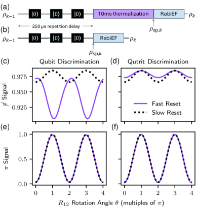
Figure 4: RabiEF with different resets. (a) Slow reset. A $10~\mathrm{ms}$ delay after the repetition delay thermalizes the transmon before the RabiEF circuits. (b) A fast reset followed by the RabiEF circuits. (c-f) Classically simulated signals with (c, e) qubit and (d, f) qutrit discrimination in the active resets in the repetition delay. Fast and slow resets are shown as solid purple and dotted black lines, respectively.

These simulation results are plotted in Figs. 4(c)-(f), with the true and estimated state-preparation probabilities in Tab. 1. Both RabiEF signals should be of the form $a\sin^{2}(b\theta)+c$ with non-negative amplitudes $a$ being physical, and all estimates $\hat{p}_{\text{sp}}$ should be valid probabilities, i.e., ${0\leq{}\hat{p}_{\text{sp}}\leq{}1}$. However, the non-negligible $\ket{2}$-state population with fast qubit reset results in a negative amplitude of the no-pi signal ($\cancel{\pi}$). This gives an incorrect negative probability estimate, see Fig. 4(c) and $\hat{p}_{\text{sp}}$ in Tab. 1. Indeed, initial states of the form

$$\rho_{\text{sp}}=(1-p_{\text{sp}}-p_{\text{sp}}^{(2)})\ket{0}\!\bra{0}+p_{\text{sp}}\ket{1}\!\bra{1}+p_{\text{sp}}^{(2)}\ket{2}\!\bra{2}$$ (12)

bias our estimate $\hat{p}_{\text{sp}}$ as

$$\hat{p}_{\text{sp}}=\frac{a_{\cancel{\pi}}}{a_{\cancel{\pi}}+a_{\pi}}=\frac{p_{\text{sp}}-p_{\text{sp}}^{(2)}}{1-3p_{\text{sp}}^{(2)}}.$$ (13)

If $p_{\text{sp}}^{(2)}$ is sufficiently large, the no-pi signal has a negative amplitude and our estimate becomes negative and unphysical . In contrast, our simulations of fast qutrit resets and slow resets are physical. Furthermore, if we look at the standard deviation of the true value $p_{\text{sp}}$, shown in Tab. 1, we see that the prepared state is more stable with fast qutrit resets and slow resets than with fast resets based on qubit discrimination. Crucially, the relative accuracy of the RabiEF with fast qutrit reset is -5.6% on a true $p_{\text{sp}}$ of $0.01206\%$.

Table 1: State-preparation errors from simulated RabiEF. The estimated probabilities $\hat{p}_{\text{sp}}$ for fast and slow resets are given, with the corresponding true probabilities $p_{\text{sp}}$. The standard errors for $\hat{p}_{\text{sp}}$ are those reported by the curve fitting software. True values are averages over the ensemble of initial states $\rho_{\text{sp},k}$ from all shots $k$ in the qutrit simulations, e.g., $\smash{p_{\text{sp}}=\operatorname{avg}_{k}\operatorname{Tr}{[\ket{1}\!\bra{1}\rho_{\text{sp},k}]}}$. True values $\smash{p_{\text{sp}}^{(2)}}$ for the $\ket{2}$ state populations are obtained with $\smash{p_{\text{sp}}^{(2)}=\operatorname{avg}_{k}\operatorname{Tr}{[\ket{2}\!\bra{2}\rho_{\text{sp},k}]}}$. Problematic cases are highlighted in bold. This includes fits that give unphysical results, $p_{\text{sp}}$ and $\hat{p}_{\text{sp}}$ that fluctuate widely, and non-negligible $\smash{p_{\text{sp}}^{(2)}}$ values.

		Fast Reset
		Qubit Reset	Qutrit Reset
$\hat{p}_{\text{sp}}$	Fit	$-0.07375362633110621$	$0.01138434338016134$
	Std. Err.	$0.002365811295332557$	$2.066484330496584\text{\times}{10}^{-06}$
$p_{\text{sp}}$	Mean	$0.02842563063242803$	$0.012064411613571418$
	Std. Dev.	$0.018402575246837197$	$1.3869525212574677\text{\times}{10}^{-05}$
$p_{\text{sp}}^{(2)}$	Mean	$0.024294292321174377$	$0.0006517619781123185$
	Std. Dev.	$0.026619774732092136$	$2.393038451362641\text{\times}{10}^{-05}$
		Slow Reset
		Qubit Reset	Qutrit Reset
$\hat{p}_{\text{sp}}$	Fit	$0.018993790238475614$	$0.018993872162638512$
	Std. Err.	$4.3537407080999903\text{\times}{10}^{-07}$	$3.982392987750876\text{\times}{10}^{-10}$
$p_{\text{sp}}$	Mean	$0.019460143125448002$	$0.01945693629988275$
	Std. Dev.	$3.913718433775682\text{\times}{10}^{-06}$	$3.2283019593791506\text{\times}{10}^{-09}$
$p_{\text{sp}}^{(2)}$	Mean	$0.0004911951199155133$	$0.0004910374920579088$
	Std. Dev.	$1.9237438001444048\text{\times}{10}^{-07}$	$1.5868437451608185\text{\times}{10}^{-10}$

These simulations demonstrate how unstable state-preparation, where $\ket{2}$ is not reset correctly, is insufficient for RabiEF. Without an accurate estimate of $p_{\text{sp}}$, separating SPAM errors in our model to mitigate dynamic circuits is not possible. Our full MCM noise learning protocol bypasses bad fast resets to obtain the estimate $\hat{p}_{\text{sp}}$, using slow resets. Though slow resets can be used for mitigation, they result in expensive circuit execution owing to their slow rates. Fast qutrit resets — even if imperfect — allow for the state-preparation characterization required to quickly split SPAM errors.

IV.2 Cycle benchmarking for readout

We now show that including an estimate of the state-preparation error in a MCB experiment results in accurate estimates of the measurement noise fidelities $f_{\text{a}}$, $f_{\text{s}}$, and $f_{\text{c}}$. We run two simulations with slow and fast resets to illustrate both noise learning paths in the full MCM noise learning protocol in Fig. 3.

The true measurement noise fidelities are set to $f_{\text{a}}=0.99096$, $f_{\text{s}}=0.99096$, and $f_{\text{c}}=0.9950$ to match the values in Sec. IV.1, see Appendix F.2. The first simulation learns $f_{\text{a}}$, $f_{\text{s}}$, and $f_{\text{c}}$ with slow state-preparation $p_{\text{sp}}^{\text{slow}}=0.01946$. Then, the fast state-preparation error probability $p_{\text{sp}}^{\text{fast}}=0.01206$ is learned with a second MCB experiment, using the now learned measurement fidelities $f_{\text{a}}$, $f_{\text{s}}$, and $f_{\text{c}}$. The first simulation splits the products of fidelities in Eq. (10) with the slow reset estimate from RabiEF, given in Tab. 1, i.e., $\hat{p}_{\text{sp}}^{\text{slow}}=0.01899$.

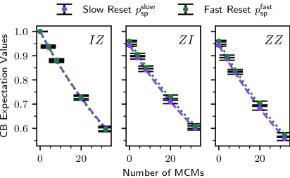
Figure 5: Measurement cycle benchmarking on a qubit. Fits to these data determine the noise channel fidelities. Error bars show the $\pm{}2\sigma$ standard errors for each expectation value. Dotted and dashed lines are obtained from non-linear least-square fits of the equation $Af^{2k}$ to the data, where $k$ is a function of the depth.

We simulated MCB with $256$ twirled-circuit randomizations for each depth $k=0,1,2,5,8$, and $128$ shots per randomization. The simulations were run with Qiskit Aer Qiskit Aer Contributors (2025), the details of which are in Appendix F.3. The resulting six decay curves are shown in Fig. 5: three per reset type, corresponding to the observables $IZ$, $ZI$, and $ZZ$ identifying the PTM entries in Eq. 10. We estimate the measurement noise fidelities by fitting decaying exponentials to the slow-reset data. The same fitting procedure is carried out for the fast reset simulation data, except that the fast reset fidelity $f_{\text{sp}}^{\text{fast}}$ is estimated using the learned measurement noise fidelities from the first simulation.

Not only does our learning procedure effectively learn the noise fidelities to less than $0.01~\%$ relative error, but we can also estimate the fast reset fidelity $f_{\text{sp}}^{\text{fast}}$ with the second MCB experiment, see Tab. 2. The state-preparation method can thus be different between full MCM noise learning and error mitigation, as long as an additional MCB experiment is run to estimate the fast state-preparation error $p_{\text{sp}}^{\text{fast}}$. This demonstrates that both paths in our full MCM noise learning protocol result in an estimate of the full noise model in Eq. 10 with split SPAM errors. An extension of our scheme to high-rate and high fidelity state preparation is discussed in Appendix G.

Table 2: Comparison of noise fidelities from simulated MCB. The estimated fidelities $\hat{f}$ are given, with their corresponding true fidelities $f$ and the relative error $\lvert f-\hat{f}\rvert/f$.

MCB with slow resets
	True $f$	Estimated $\hat{f}$	Rel. Error
$f_{\text{a}}$	$0.99096$	$0.99101$	$5.637\times{}10^{-5}$
$f_{\text{s}}$	$0.99096$	$0.99022$	$7.460\times{}10^{-4}$
$f_{\text{c}}$	$0.99500$	$0.99570$	$7.055\times{}10^{-4}$
Second MCB experiment with fast resets
	True $f$	Estimated $\hat{f}$	Rel. Error
$f_{\text{sp}}^{\text{fast}}$	$0.97588$	$0.97676$	$9.061\times{}10^{-4}$

IV.3 Example mitigation of final readout errors

We now show classical simulations of our method on the stabilizer circuit in Fig. 1(a). The simulations use the same slow reset fidelity as in Secs. IV.1 and IV.2, and implement both TREX and the mitigation from Eq. 1. These simulations, done with Qiskit Aer, do not simulate leakage, as the $\ket{2}$-state is assumed negligible for all experiments except RabiEF.

The TREX mitigator $\langle{}Z^{\star}\rangle$ is learned with $16$ twirling randomizations and $5000$ shots per randomization, for $n=4,6,8,10$ qubits, i.e., the same as in Sec. II. The measurement and state-preparation noise fidelities were taken from Sec. IV.2. The stabilizer circuit was simulated for $n=4,6,8,10$ qubits, with $128$ shots per twirling randomization, and $2^{10}\times{}n^{2}$ total shots. With the hardware experiments, we compare our mitigated results to Clifford simulations with CNOT noise. By contrast, here we assume ideal gates to compare the mitigated expectation values to their ideal value of $+1$, the dashed green line in Fig. 6. The expected result with TREX is $f_{\text{sp}}^{1-n}$, shown by the dashed purple line in Fig. 6.

As seen in the hardware experiments, TREX overshoots the ideal expectation values by a factor $f_{\text{sp}}^{1-n}$, see purple dots in Fig. 6. This is expected since $\langle Z^{\star}\rangle$ picks-up the same factor from imperfect state-preparation, i.e., the purple dashed line. If, however, the values are mitigated with Eq. 1, then the expectation values do not overshoot, and instead lie around the ideal value of $\langle{}O\rangle{}=+1$, see green dots in Fig. 6. This shows a correct mitigation of SPAM errors, further validating the error mitigation employed in Sec. III.

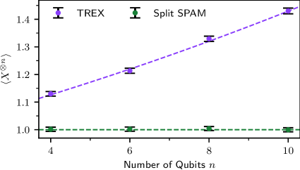
Figure 6: Mitigation of the $\langle X^{\otimes n}\rangle$ expectation value. The values are mitigated with TREX and the modified mitigator from the hardware experiments, which splits state-preparation and measurement errors (“Split SPAM”). Error bars show the $\pm{}2\sigma$ standard errors for each mitigated expectation value. Dashed lines show the expected expectation values given knowledge of the simulated GHZ state preparation circuit. The green dashed line shows the noiseless expectation value of $+1$.

IV.4 Example mitigation of dynamic circuits

Splitting SPAM errors is most beneficial with mid-circuit measurements, where measurement noise can be mitigated separately from state-preparation and gate noise. We demonstrate that our MCM noise learning protocol helps mitigate errors in dynamic circuits. In particular, we simulate a noisy three-qubit teleportation circuit and mitigate SPAM errors with PEC Van Den Berg et al. (2023); Gupta et al. (2024) built on our noise learning protocol. The circuit is constructed in the CNOT picture, i.e., including the classical bits as is done in Fig. 2, and simulated with Qiskit Aer Qiskit Aer Contributors (2025). The teleportation circuit, shown in Fig. 7, includes explicit noise channels for state-preparation $\Lambda_{\text{sp}}$, measurement assignment $\Lambda_{\text{a}}$, state $\Lambda_{\text{s}}$, and correlated $\Lambda_{\text{c}}$ errors, as defined in Sec. III. The underlying fidelities $f_{\text{x}}$ are taken from Sec. IV.2, with a state-preparation fidelity $f_{\text{sp}}=0.96108$ equivalent to the slow resets.

The ideal teleported state

$$\rho_{\text{in}}^{\text{ideal}}=\ket{\psi}\!\!\bra{\psi}=R_{X}(\theta)\ket{0}\!\!\bra{0}R_{X}^{\dagger}{}(\theta).$$ (14)

is prepared by an $R_{X}$ gate with rotation angle $\theta\in[0,2\pi]$. However, SPAM noise introduce errors into the final teleported state on qubit $\text{q}_{2}$.

To apply PEC, we generate $128$ PEC circuit realizations, replacing the inverse channels $\tilde{\Lambda}^{-1}$ with Paulis from their quasi-probability distribution representations. Each circuit is then simulated, resulting in $128$ noisy teleported states $\rho_{\text{out},j}$ on qubit $\text{q}_{2}$, with $j\in[0,127]$. As PEC mitigates expectation values and not states, we obtain mitigated states via state tomography. From each noisy teleported state $\rho_{\text{out},j}$, we obtain three ideal Pauli expectation values

$$\langle{}P\rangle{}_{j}=\operatorname{Tr}[P\rho_{\text{out},j}],$$ (15)

for Paulis $P=X,Y,Z$. We emulate shot-noise by sampling $100$ times, per circuit realization, from the corresponding Bernoulli distributions, resulting in expectation values $E_{P,j}$ impacted by both SPAM and shot noise. The PEC mitigated expectation values are then

$$\langle{}P\rangle{}_{\text{mit}}=\gamma\sum_{j}(-1)^{m_{j}}E_{P,j}$$ (16)

where $\gamma$ is the noise factor for the inverse noise channels and $m_{j}$ is an integer from PEC controlling how the quasi-probability inverse channels are engineered Van Den Berg et al. (2023); Gupta et al. (2024). Physical states are obtained from state tomography by minimizing a mean-squared error as follows:

$$\rho_{\text{mit}}=\operatorname*{arg\,min}_{\rho_{t}}\sum_{P=X,Y,Z}\left(\operatorname{Tr}[P\rho_{t}]-\langle{}P\rangle{}_{\text{mit}}\right)^{2}.$$ (17)

Here, the state $\rho_{t}$ is parameterized as

$$\rho_{t}=\rho(t_{1},t_{2},t_{3},t_{4})=\frac{T^{T}T}{\operatorname{Tr}[T^{T}T]},$$ (18)

with real parameters $t_{1}$, $t_{2}$, $t_{3}$, $t_{4}$, and triangular matrix

$$T=\begin{pmatrix}t_{1}&0\\ t_{3}+it_{4}&t_{2}\end{pmatrix}.$$ (19)

This ensures a physical mitigated state $\rho_{\text{mit}}$ for a given ensemble of PEC circuit realizations. We then compute the state fidelity

$$\mathcal{F}(\rho_{\text{in}}^{\text{ideal}},\rho_{\text{mit}})=\operatorname{Tr}\!\left[\sqrt{\sqrt{\rho_{\text{in}}^{\text{ideal}}}\rho_{\text{mit}}\sqrt{\rho_{\text{in}}^{\text{ideal}}}}\right]^{2}$$ (20)

as a metric of success. This is done for $300$ realizations of the simulation and $15$ rotation angles in the input state, see Fig. 8. The unmitigated case does not need PEC and is thus simulated as a single circuit directly resulting in a physical state. Therefore, the state fidelity is computed on the output state $\rho_{\text{out}}$ directly, instead of using state tomography.

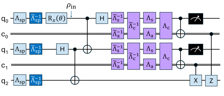
Figure 7: Teleportation Circuit in the CNOT picture. The circuit includes state-preparation noise $\Lambda_{\text{sp}}$ and measurement noise $\Lambda_{\text{s}}$, $\Lambda_{\text{a}}$, and $\Lambda_{\text{c}}$. Inverse channels $\tilde{\Lambda}^{-1}$ are implemented by sampling their quasi-probability distributions for PEC. The output state $\rho_{\text{out}}$ is the state of the last qubit $q_{2}$, i.e., with the other qubits and classical bits traced out. The state to be teleported is $\rho_{\text{in}}$, which is affected by the state-preparation noise $\Lambda_{\text{sp}}$ of qubit zero and its inverse channel $\tilde{\Lambda}_{sp}^{-1}$.

Figure 8: State fidelities for unmitigated and PEC mitigated teleportation circuits. PEC is used to mitigate Pauli expectation values which are then used with state-tomography to estimate the state infidelity. The median mitigated state infidelities are shown in green, over $300$ random realizations of the simulation. Error-bars show the interquartile range over the $300$ realizations. The unmitigated fidelities, in purple, are computed directly on the unmitigated state $\rho_{out}$ without PEC samples or state tomography.

The PEC mitigated state fidelities are significantly higher than the unmitigated values, showing that we are mitigating SPAM errors, see Fig. 8. The majority of the $300$ simulation realizations result in state-fidelities above $98~\%$, whereas the best-case unmitigated fidelity is less than $96~\%$. We also confirm that PEC effectively mitigates both state-preparation and measurement errors separately by rerunning the simulations with only one of the error sources, still observing improvements to the state fidelities with PEC (data not shown). Our MCM noise learning procedure thus effectively splits SPAM errors, facilitating PEC mitigation of dynamic circuits. Splitting SPAM errors was made possible by learning the state-preparation fidelity $p_{\text{sp}}$ using non-computational states with a RabiEF experiment.

V Discussion and Conclusion

Our experimental data show how state-preparation errors prevent the accurate mitigation of SPAM errors for certain expectation values, corroborating recent results Chen et al. (2025a). A passive reset of the qubits into a thermal state, whose population we measure with non-computational states, allows us to resolve this by mitigating state-preparation errors independently of measurement errors. This prevents the unphysical behavior seen in some TREX-mitigated expectation values.

We introduce a noise model of (mid-)circuit measurements which fully accounts for state-preparation errors and errors in the final measurement. This extends recent noise learning protocols, such as Ref. Zhang et al. (2025), by learning the state-preparation error independently of measurement noise. Our work also complements a recently introduced noise learning framework that learns state-preparation, gate, and measurement noise is a self-consistent way up to unlearnable gauge degrees of freedom Chen et al. (2024). While this protocol also resolves the aforementioned issues of TREX Chen et al. (2025a), the unconstrained degrees of freedom render it unsuitable for dynamic circuits. With the added resource of non-computational states, we learn the ground truth of the state-preparation error. Crucially, our noise learning then allows us to mitigate errors that occur in dynamic circuits which explicitly require MCMs and feedforward gates. We successfully demonstrate this with simulations of a teleportation circuit. As an outlook, we propose to combine our state-preparation learning with the formalism from Refs. Chen et al. (2024, 2025a). This will fully constrain the self-consistent noise models by anchoring the gauge, thus significantly broadening their scope.

We propose to learn the state-preparation error with a RabiEF experiment which requires either a slow passive reset or a fast active qutrit reset. This fits well with recent developments since error correction requires a strong suppression of leakage which can be achieved through appropriate qutrit resets Battistel et al. (2021); Miao et al. (2023). Importantly, our work requires the transmon to stay within its first three levels. Therefore, we do not capture effects where the transmon may escape from this subspace Khezri et al. (2023) or even confined states Lescanne et al. (2019). Here, we believe that operating transmons in such regimes should be avoided.

Our work leverages a non-computational state of transmon qubits. However, the work should generalize to other hardware platforms that have non-computational states. These may be found in, for instance, solid state electron spin qutrits Fu et al. (2022); Guo et al. (2024) and trapped ions Klimov et al. (2003). An analytical treatment of the impact of all errors in the measurements and how they propagate to the mitigated observables would be a useful extension of the numerical analysis in Appendix A.2. In addition, future work may also explore generalizations of the qubit readout model to a full qutrit model and the subsequent impact on noise learnability.

In summary, non-computational states allow us to overcome no-go theorems that hold when the learning framework is restricted to the computational sub-space. As a result, we can fully specify degrees of freedom of noise models that are fundamentally unlearnable when restricted to qubit circuits. We illustrate this by separately mitigating state and preparation errors. Crucially, this is also possible without a slow passive reset of the quantum computer when a noisy qutrit reset is available.

Note added While completing this project, we became aware of related work by S. Chen et al. Chen et al. (2025b), in which the authors also leverage non-computational states of the transmon.

VI Acknowledgements

The authors acknowledge M. Mergenthaler, A. Fuhrer, and L. C. G. Govia, M. Takita, and A. Seif for useful discussions. This work was supported as a part of NCCR SPIN, a National Centre of Competence in Research, funded by the Swiss National Science Foundation (grant number 225153). D.J.E. acknowledges funding within the HPQC project by the Austrian Research Promotion Agency (FFG, project number 897481) supported by the European Union – NextGenerationEU. L.E.F. acknowledges funding from the European Union’s Horizon 2020 research and innovation program under the Marie Skłodowska-Curie grant agreement No. 955479 (MOQS – Molecular Quantum Simulations).

Appendix A Measuring thermal state population

The RabiEF experiment measures the population $\alpha$ in the excited state of the qubit for a state $\rho=(1-\alpha)\ket{0}\!\bra{0}+\alpha\ket{1}\!\bra{1}$ Geerlings et al. (2013). RabiEF drives oscillations in the $\{\ket{1},\ket{2}\}$ subspace with a $R_{12}(\theta)$ gate which rotates around the $X$-axis of the corresponding Bloch sphere. Measuring $\alpha$ requires two independent experiments called $\pi$ and no-$\pi$, indicated by $\cancel{\pi}$. In the $\pi$-experiment we apply the gate sequence $X-R_{12}(\theta)-X$ while the no-$\pi$-experiment omits the first $X$ gate. The difference between both experiments is thus the $\pi$-pulse on the thermal state at the beginning of the gate sequence. Following this gate sequence, which we assume is ideal, we apply a noisy measurement with discrimination errors. This results in two oscillating signals $s_{\pi}(\theta)$ and $s_{\cancel{\pi}}(\theta)$ which we fit to two independent functions of the form $a\sin^{2}(\theta+c)+b$, see Fig. 1(d). Here, $a$, $b$, and $c$ are the fit parameters. Finally, the excited state population $\alpha$ is estimated by

$$\hat{\alpha}=\frac{a_{\cancel{\pi}}}{a_{\cancel{\pi}}+a_{\pi}}$$ (21)

where $a_{\cancel{\pi}}$ and $a_{\pi}$ are the amplitudes of the function that fit $s_{\cancel{\pi}}(\theta)$ and $s_{\pi}(\theta)$, respectively. In practice, we implement $R_{12}(\theta)$ with a Rabi pulse $R_{12}(A)$ of amplitude $A\propto{}\theta$. The exact relationship between $A$ and $\theta$ is irrelevant, as it only controls the frequency of the RabiEF signals, and not their amplitudes.

Superconducting qubit measurements return complex values in the IQ plane Krantz et al. (2019) to which we apply a principal component analysis to forgo classification and instead use the projected signals $s_{\pi}^{\prime}(A)\propto{}s_{\pi}(\theta)$ and $s_{\cancel{\pi}}^{\prime}(A)\propto{}s_{\cancel{\pi}}(\theta)$. These signals have arbitrary units and can be larger than $1$ owing to the location of the reference points in the IQ plane, see Fig. 1(d). Crucially, gate and measurement errors tend to cancel out in Eq. 21 as they affect $a_{\pi}$ and $a_{\cancel{\pi}}$ in the same way.

A.1 Thermal state populations

Here, we discuss the experimental thermal state data presented in Fig. 1 which is taken on qubits 114 to 121 on the IBM Quantum device ibm_pinguino3. The thermal populations of these qubits are measured with RabiEF after a $10~{\rm ms}$ passive reset. The resulting $\ket{1}$ state population $\alpha$ ranges from $3.06$ to $8.75~\%$, see Tab. 3, and creates a significant state-preparation error. From the measured population $\alpha$ in the $\ket{1}$ state we compute an effective qubit temperature $T_{\text{eff}}$ following the relation $\alpha=\exp[-\hbar\omega_{01}/(k_{b}T_{\text{eff}})]$. The resulting effective temperatures, shown in Tab. 3, are larger than the ${\sim 15~{\rm mK}}$ of dilution refrigerators. We then use the above relation to estimate the population in the second excited state by replacing $\omega_{01}$ with $2\omega_{01}+\Delta$, where $\Delta$ is the transmon anharmonicity. The resulting populations $\beta$ are at least an order of magnitude lower than their corresponding populations $\alpha$ in the first excited state. This justifies the assumption that the $\ket{2}$-state population is negligible when slow resets are used.

Table 3: Properties of qubits used in the data presented in Fig. 1 of the main text. The qubit frequency is $\omega_{01}$. The transmon anharmonicity is $\Delta$. The population in the $\ket{1}$ state measured with RabiEF is $\alpha$. The inferred population in the second excited state is $\beta$.

Qubit	114	115	116	117	118	119	120	121
$\omega_{01}/(2\pi)~({\rm GHz})$	5.14	5.22	5.08	5.22	5.28	5.16	5.03	5.15
$\Delta/(2\pi)~({\rm MHz})$	-303	-303	-304	-302	-303	-304	-305	-302
$\alpha~(\%)$	4.99	8.75	4.01	6.00	4.17	3.06	5.42	2.79
$T_{\text{eff}}~({\rm mK})$	82	103	76	89	80	71	83	69
$\beta~(\%)$	0.30	0.88	0.19	0.42	0.21	0.11	0.35	0.10
$T_{1}~(\mu{\rm s})$	281	259	207	222	199	293	175	261

A.2 RabiEF and assignment errors

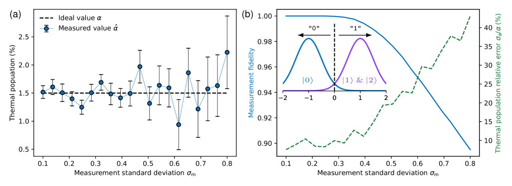
Figure 9: Sensitivity of RabiEF on assignment errors. (a) Simulations of estimates of $\ket{1}$ state population $\alpha$ with 300 shots per data point. The error bars are obtained by propagating fit errors on $a_{\pi}$ and $a_{\cancel{\pi}}$ through Eq. (21). The dashed horizontal line shows the ideal value $\alpha=1.5\%$. (b) The solid line shows how the readout fidelity $F$ varies with $\sigma_{\text{m}}$. The green dashed line shows how the error bars from panel (a), normalized to $\alpha$, grow with the strength of assignment errors $\sigma_{\text{m}}$ for a fixed 300 shots per $\hat{\alpha}$. The inset shows how the three states are assigned to labels "0" and "1".

We provide numerical evidence that the RabiEF measurement of $\alpha$ is accurate despite measurement assignment errors. We construct a three level model with states $\ket{0}$, $\ket{1}$, and $\ket{2}$. The initial state is the thermal state $\rho_{\text{th}}=(1-\alpha)\ket{0}\bra{0}+\alpha\ket{1}\bra{1}$ where we assume that the thermal population in $\ket{2}$ is negligible. The gates in the RabiEF circuits are assumed ideal. Crucially, we add finite sampling effects and discrimination errors in the readout process with a discrimination in a one-dimensional space with overlapping Gaussians.

Here, the state $\ket{0}$ is mapped to a Gaussian distribution $\mathcal{N}(\mu=-1,\sigma_{\text{m}})$ with mean $-1$ and standard deviation $\sigma_{\text{m}}$. The $\ket{1}$ and $\ket{2}$ states are mapped to a single Gaussian distribution $\mathcal{N}(\mu=1,\sigma_{\text{m}})$ with mean $+1$ and standard deviation $\sigma_{\text{m}}$. To draw a shot from a state $\rho$ we first chose a random number $\mu$ from $\{-1,1\}$ where the probability of $-1$ is $\operatorname{Tr}[\rho\ket{0}\!\!\bra{0}]$ and the probability of $+1$ is $\operatorname{Tr}[\rho(\ket{1}\!\!\bra{1}+\ket{2}\!\!\bra{2}]$. Next, we mimic the readout process by sampling from $\mathcal{N}(\mu,\sigma_{\text{m}})$ and assigning a count of 1 if the result is greater than 0. Therefore, the overlap between the two Gaussian distributions $\mathcal{N}(\mu=-1,\sigma_{\text{m}})$ and $\mathcal{N}(\mu=1,\sigma_{\text{m}})$ — controlled by $\sigma_{\text{m}}$ — creates measurement assignment errors, see inset in Fig. 9(b). The relation between $\sigma_{\text{m}}$ and the readout fidelity $F=1-[P(1|0)+P(0|1)]/2$ is shown in Fig. 9(b).

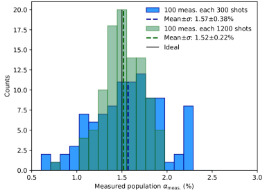
Figure 10: Increasing shots improves RabiEF precision. Distribution of 100 individual measurements of $\alpha$ with 300 and 1200 shots. Here, $\sigma_{\text{m}}=0.6$ which corresponds to a readout error of 4.8%. By comparison, the mean readout error on ibm_fez is 1.7%.

Even in the presence of strong assignment errors, e.g., $\sigma_{\text{m}}>0.4$ for which $F<99\%$, RabiEF accurately measures $\alpha$. The estimates $\hat{\alpha}$ center around the ideal value set to $1.5~\%$, see Fig. 9(a). Furthermore, the magnitude of the error bars, correspondingly the standard deviation of the distribution of independent measures, increases with the assignment error, see Fig. 9(b). Crucially, we can reduce these errors by increasing the number of shots, see Fig. 10. Here, the distribution of measurements is again centered around the ideal value. Importantly, increasing the shots reduces the variance of the distribution.

These results are expected given assignment errors, and potentially other imperfections, affect both $a_{\pi}$ and $a_{\cancel{\pi}}$. Therefore, as $\alpha$ is estimated with a ratio where both numerator and denominator depend linearly on the fitted amplitudes we can expect the measurement to be first-order insensitive to assignment errors.

Appendix B Error propagation

Here, we give details on the computation of the error bars shown in Fig. 1. The uncertainty is calculated via standard error propagation. For example, the propagated standard deviation on $\langle O\rangle_{\text{mit}}$ is

$$\sigma_{\text{mit}}^{2}= \left(\frac{\partial\langle O\rangle_{\text{mit}}}{\partial\langle O\rangle_{\text{raw}}}\sigma_{\text{raw}}\right)^{2}+\left(\frac{\partial\langle O\rangle_{\text{mit}}}{\partial\langle Z^{\star}\rangle}\sigma_{\langle Z^{\star}\rangle}\right)^{2}$$

$$+ \sum_{i=1}^{n-1}\left(\frac{\partial\langle O\rangle_{\text{mit}}}{\partial f_{\text{sp},i}}\sigma_{\text{sp},i}\right)^{2}.$$ (22)

Here, $\sigma_{\langle Z^{\star}\rangle}$ denotes the standard deviation on the TREX denominator. The standard deviations for observables $O$, i.e., $\sigma_{\text{raw}}$ and $\sigma_{\langle Z^{\star}\rangle}$, are computed from the samples based on $\langle O^{2}\rangle-\langle O\rangle^{2}$. The standard deviation $\sigma_{\text{sp},i}$ from the RabiEF experiment on qubit $i$ is based on the uncertainties stemming from the underlying curve fits.

Appendix C CNOT noise

The shaded area in Fig. 1 represents the range of possible values for the observable when only CNOT noise is present, i.e., the raw observable after removing SPAM errors and assuming no out-of-model errors. To obtain this shaded area, first, we twirl the two-qubit gates and learn a sparse Pauli-Lindblad noise model for the two layers $L_{1}$ and $L_{2}$ in Fig. 1(b) following Ref. Van Den Berg et al. (2023). Next, we use the resulting noise model to compute the noisy observable via a classical Clifford simulation which contains only the noise for the CNOT gates. Crucially, the error rates of conjugate Pauli pairs, i.e., $P$ and $UPU^{\dagger}$ (where $P$ is a Pauli and $U$ the unitary of the CNOT layer) can only be inferred as a product by this noise learning protocol. However, the simulation requires specifying individual rates which introduces degrees of freedom. Initially, we split the product symmetrically, as supported by recent theoretical work up to leading order Malekakhlagh et al. (2025). Finally, we solve two optimization problems that adjust the splits of conjugate Pauli pairs to either maximize or minimize the measured observable under the constraint of all Pauli fidelities remaining physical, i.e., $\leq 1$. This results in the shaded area in Fig. 1(e). As these optimization problems are non-convex, we don’t know whether the solutions we find are the global optima. This may also explain why the data on four qubits in Fig. 1(c) lies outside of the gray area. We have opted for this procedure out of simplicity as it suffices to highlight the importance of separating state-preparation and measurement noise. The resulting spread in possible observable values is large. With additional noise learning circuits, the noise model of the CNOT gate layers could be further constrained by implementing interleaved cycle benchmarking Chen et al. (2023a), multi-layer cycle benchmarking Calzona et al. (2024), or a self-consistent gate set learning scheme Chen et al. (2024).

Appendix D Pauli transfer matrices

For completeness, we now provide a definition of Pauli Transfer Matrices (PTM) Greenbaum (2015). They provide a useful representation of quantum channels. The elements of the PTM of an $n$-qubit quantum channel $\Lambda$ are

$$\left(\Gamma_{\Lambda}\right)_{ij}=\frac{1}{2^{n}}\operatorname{Tr}[P_{i}\Lambda(P_{j})],$$ (23)

where $[P_{0},\ldots,P_{4^{n}-1}]$ denotes the $n$-qubit Pauli basis arranged in lexicographic order. The PTM of a composite map $H\circ G$ is the matrix product of the PTMs of the individual maps $\Gamma_{H}\Gamma_{G}$. Therefore, the assumption that noise $\Lambda_{G}$ occurs before a gate $G$ translates to PTMs as $\Gamma_{G}\Gamma_{\Lambda_{G}}$.

Next, the PTM of a measurement is a matrix whose only nonzero entries are $1$’s in the top-left and bottom-right corners, with all other entries equal to $0$. As a result, it annihilates any prior $X$ or $Y$ components of an operation. Consequently, our PTMs are defined as above, but with the basis restricted to the set $\{I,Z\}^{\otimes n}$ arranged in lexicographic order. As an example, consider the one-qubit channel $\Lambda(\rho)=(1-p)\rho+pX\rho X$. Its PTM in the full basis $\{I,X,Y,Z\}$ is

$$\Gamma_{\Lambda}=\begin{pmatrix}1&0&0&0\\ 0&1&0&0\\ 0&0&1-2p&0\\ 0&0&0&1-2p\\ \end{pmatrix}.$$ (24)

Since we consider only the $\{I,Z\}$ part of the basis we express this PTM as

$$\Gamma_{\Lambda}=\begin{pmatrix}1&0\\ 0&1-2p\\ \end{pmatrix}.$$ (25)

Finally, an important property of PTMs combined with twirling is that twirling transforms any noise channel into a Pauli noise channel, resulting in a diagonal PTM.

Appendix E PTM of final measurements

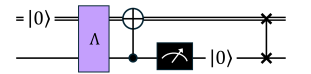
Figure 11: In the CNOT picture, the final measurement corresponds to measuring the control qubit. The outcome is written back onto the qubit (control) wire, which thereafter functions as a classical line.

In a final measurement - i.e., measuring the control qubit in the CNOT picture - the outcome is written back onto the same wire, which then acts as a classical bit. To derive the corresponding PTM, we temporarily introduce an ancillary classical line and decompose the measurement into the following sequence, also shown in Fig. 11. (i) Apply an ideal reset to the ancillary classical line to initialize it in the $0$ state. (ii) Apply the noisy measurement in the CNOT picture by transferring the control-qubit outcome onto the ancillary line. (iii) Reset the qubit wire, which from this point on acts as a classical line. (iv) Swap the value from the ancillary classical line back onto the (now classical) qubit wire. (v) Remove the ancillary classical line. We compute the PTMs of each component in this circuit and multiply them to obtain the PTM for the final noisy measurement. The PTM of a reset operator $\mathcal{R}(\rho)=E_{0}\rho E_{0}^{\dagger}+E_{1}\rho E_{1}^{\dagger}$, where $E_{0}=\ket{0}\!\!\bra{0}$ and $E_{1}=\ket{0}\!\!\bra{1}$, is

$$\Gamma_{\ket{0}}=\begin{pmatrix}1&0\\ 1&0\\ \end{pmatrix}.$$ (26)

The PTM of the SWAP is

$$\Gamma_{\text{SWAP}}=\begin{pmatrix}1&0&0&0\\ 0&0&1&0\\ 0&1&0&0\\ 0&0&0&1\\ \end{pmatrix}.$$ (27)

The PTM of a final measurement can then be calculated as $\Gamma_{\text{fm}}=\Gamma_{\text{SWAP}}\left(\Gamma_{\ket{0}}\otimes I\right)\Gamma_{\text{CX}}\Gamma_{\Lambda}\left(I\otimes\Gamma_{\ket{0}}\right)$ where $\Gamma_{\text{CX}}\Gamma_{\Lambda}$ is defined in Eq. 6, and $\Gamma_{\ket{0}}$ and $\Gamma_{\text{SWAP}}$ are defined in Eq. 27 and Eq. 26, respectively. The result is

$$\Gamma_{\text{fm}}=\begin{pmatrix}1&0\\ 0&f_{a}f_{s}\\ \end{pmatrix}\otimes\begin{pmatrix}1&0\\ 1&0\\ \end{pmatrix}.$$ (28)

Here, $f_{\text{a}}$ and $f_{\text{s}}$ are, as before, the fidelity of the assignment and state errors, respectively. Thus, after discarding the ancillary classical line, the PTM of a final noisy measurement is $\text{diag}(1,f_{\text{a}}f_{\text{s}})$. The absence of $f_{\text{c}}$ in this PTM is understood as follows. The correlated error simultaneously flips the qubit and the classical bit. For example, a qubit, initially in state $\ket{0}$, is measured as $1$, and the qubit ends up in $\ket{1}$. However, in final measurements we are only concerned with the correctness of the reported outcome. Thus, such an event is effectively indistinguishable from a simple bit-flip error and can be interpreted either as a readout assignment error or a state-preparation error.

Appendix F Setup of simulations

Our simulations fall into two categories, qubit and qutrit simulations. As the RabiEF experiment uses gates that interact with the $\ket{2}$ state it is the only experiment simulated with qutrits. Appendix F.1 describes our qutrit simulator and its application to the RabiEF experiment. Appendix F.2 translates the readout assignment matrix $R$ to the measurement noise fidelities. Appendix F.3 discusses the setup of qubit simulations for the results shown in Sec. IV.2 and Sec. IV.3. Appendix F.4 gives details on the simulation of the teleportation circuit, including PEC.

F.1 Qutrit simulations for RabiEF

To simulate the RabiEF experiments while taking into account the $\ket{2}$-state population, we implemented a qutrit simulator with Qiskit Javadi-Abhari et al. (2024). All qubit instructions are embedded as ideal gates in $SU(3)$, and thus do not interact with the $\ket{2}$ state. Only the $R_{12}(\theta)$ and $X_{12}$ gates, noise channels, and measurements interact with the $\ket{2}$-state. The circuits are converted into a series of operators, i.e., SuperOp class instances with qutrit dimensions. For example, a single qutrit error channel is a $9\times{}9$ superoperator matrix. A state $\rho$ is evolved by a circuit $c$ by repeatedly calling the DensityMatrix.evolve(op, qargs) Qiskit method, where the op argument is the operator for each gate and qargs is a list of qutrit indices identifying the support of the operator. A RabiEF experiment consists of three circuits: the two $\cancel{\pi}$ and $\pi$, circuits $c_{\cancel{\pi}}$ and $c_{\pi}$, respectively, and a repetition delay circuit $c_{\text{rep}}$ consisting of three active resets and an optional delay for slow resets. The delay is not simulated when fast resets are used. The simulator evolves an initial state $\rho=(\ket{0}\!\bra{0})^{\otimes{}n}$ by simulating the circuits in the following loop $N$ samples many times: (i) apply $c_{\text{rep}}$, (ii) apply $c_{\cancel{\pi}}$, (iii) apply $c_{\text{rep}}$, and (iv) apply $c_{\pi}$. One loop corresponds to a single sample per $\cancel{\pi}$ and $\pi$ circuit. Both RabiEF circuits $c_{\cancel{\pi}}$ and $c_{\pi}$ produce measurement outcomes which are stored in two length-$N$ arrays. The repetition delay also produces measurement outcomes, but they are only used to control the feedforward instructions in the active resets and are not stored long-term. The initial states for each circuit, $\rho_{\text{in},k}$, over all $k$ samples are saved to compute the true state-preparation probability $p_{\text{sp}}$, shown in Tab. 1, as

$$p_{\text{sp}}\coloneqq\underset{\begin{subarray}{c}s=\cancel{\pi},\pi\\ k=0,\ldots{},N-1\end{subarray}}{\operatorname{avg}}\operatorname{Tr}\left[\ket{1}\!\bra{1}\rho_{\text{in},k}^{(s)}\right].$$ (29)

We simulate thermal relaxation during slow resets, measurements, and idle times in the repetition delay. Noise channels for measurements are applied before the ideal measurement. We numerically compute the thermal relaxation channel with the Lindblad master equation and six Lindblad operators defining relaxation, heating, and dephasing. Each Lindblad operator $L_{i}$ has a corresponding rate $\gamma_{i}$, controlling the strength of the operator. The operators and rates are

$$L_{1} =\ket{0}\!\bra{1}, L_{2} =\ket{1}\!\bra{0},$$ (30)

$$L_{3} =\ket{1}\!\bra{2}, L_{4} =\ket{2}\!\bra{1},$$

$$L_{5} =\ket{0}\!\bra{0}-\ket{1}\!\bra{1}, L_{6} =\ket{1}\!\bra{1}-\ket{2}\!\bra{2},$$

$$\gamma_{1} =\frac{1}{T_{1}}, \gamma_{2} =\gamma_{1}\exp({-\hbar\omega_{01}/k_{B}T_{\text{eff}}})$$ (31)

$$\gamma_{3} =\frac{1}{T_{1}^{12}}, \gamma_{4} =\gamma_{3}\exp({-\hbar(\omega_{01}+\Delta)/k_{B}T_{\text{eff}}})$$

$$\gamma_{5} =\frac{1}{T_{2}}, \gamma_{6} =\frac{1}{T_{2}^{12}}.$$

The solution to the Lindblad master equation $\Lambda_{\text{th}}(\rho,t)$ for a given evolution time $t$ is computed with Qiskit Dynamics Puzzuoli et al. (2023) and included as a SuperOp instruction in the circuits. The rates $\gamma_{1}$, $\gamma_{3}$, $\gamma_{5}$, and $\gamma_{6}$ are chosen from typical superconducting qubit decoherence times Dane et al. (2025), with their definitions given in Eq. 31 and their values in Tab. 4. The heating rates $\gamma_{2}$ and $\gamma_{4}$ are calculated using the energy differences between $\ket{0}$, $\ket{1}$, and $\ket{2}$, and an assumed effective qutrit temperature $T_{\text{eff}}=60~{\rm mK}$ following the Boltzmann distribution. We further assume that the qutrits decay sequentially, i.e., $\ket{2}$-$\ket{0}$ transitions are naturally suppressed by the quantum hardware Fischer et al. (2022). We include measurement-induced leakage with an additional error channel prior to the ideal measurements, after the measurement-associated thermal relaxation. This is modelled as a projection to the $\ket{2}\!\bra{2}$ state with probability $p_{\text{leak}}=0.2~\%$. The error channel on a qubit undergoing measurement, with duration $t_{\text{meas}}=1244~\mathrm{ns}$, is thus

$$\Lambda_{\text{meas}}(\rho)=(1-p_{\text{leak}})\Lambda_{\text{th}}(\rho,t_{\text{meas}})+p_{\text{leak}}\ket{2}\!\!\bra{2}.$$ (32)

Following this noise channel, our simulator applies an ideal projective measurement and then the readout assignment matrix $R$, see Appendix F.2 and Eq. 11. The simulator then records the noisy measurement outcome as the integer $o=0,1,2$ and uses the post-measurement state as the input to the next circuit. Qutrit discrimination is only used for measurements in the repetition delay, as RabiEF requires binary classification.

Table 4: Parameters used in the simulations.

Symbol	Value	Description
$T_{\text{eff}}$	$60~{\rm mK}$	Qubit Effective Temperature
$T_{1}$	$200~\mu{}{\rm s}$	Relaxation time in the qubit subspace
$T_{2}$	$100~\mu{}{\rm s}$	Dephasing time in the qubit subspace
$T_{1}^{12}$	$100~\mu{}{\rm s}$	Relaxation time in the qutrit subspace
$T_{2}^{12}$	$50~\mu{}{\rm s}$	Dephasing time in the qutrit subspace
$\omega_{01}$	$4.9~{\rm GHz}$	Qubit $0$-$1$ frequency
$\Delta$	$-0.3~{\rm GHz}$	Qubit anharmonicity
$t_{\text{rep. delay}}$	$250~\mu{}{\rm s}$	Repetition delay time
$t_{\text{meas}}$	$1244~{\rm ns}$	Measurement time
$P_{\text{leak}}$	$0.2~\%$	Prob. to leak during a measurement

F.2 Assignment error fidelities for qutrits

Errors in final measurements can be specified as a readout assignment error matrix where entry $j,k$ is the probability $q_{jk}$ to misclassify state $\ket{k}$ as $\ket{j}$. The $3\times 3$ qutrit readout assignment matrix

$$R=\begin{pmatrix}q_{00}&q_{01}&q_{02}\\ q_{10}&q_{11}&q_{12}\\ q_{20}&q_{21}&q_{22}\\ \end{pmatrix}$$ (33)

used in the RabiEF simulation is based on existing hardware experiments Fischer et al. (2022); Chen et al. (2023b); Kanazawa et al. (2023). We thus neglect the overlap between the $\ket{0}$ and $\ket{2}$ readout signals, i.e., $q_{02}=q_{20}=0$, and assume that the qutrit misclassification probability for $\ket{1}$-$\ket{2}$ is approximately an order of magnitude larger than for $\ket{0}$-$\ket{1}$. Therefore, we set $q_{12}=6~\%$ and $q_{01}=0.9~\%$ resulting in the readout assignment matrix shown in Eq. 11.

When qubit reset is used, we require a readout assignment matrix that always misclassifies $\ket{2}$ as $\ket{1}$, see Eq. 11. The qubit readout assignment errors $p_{jk}$ are related to the qutrit ones following

$$p_{00} =q_{00}$$ (34a)

$$p_{11} =q_{11}+q_{21}$$ (34b)

$$p_{01} =q_{01}$$ (34c)

$$p_{10} =q_{10}+q_{20}$$ (34d)

with $q_{20}=0$ as discussed above. From the values in Eq. 11 we obtain qubit assignment matrix probabilities $p_{00}=p_{11}=99.1~\%$ and $p_{01}=p_{10}=0.9~\%$.

To ensure consistency between the RabiEF simulations in Sec. IV.1 and Sec. IV.2 we now connect the qubit readout assignment matrix $p_{jk}$ to the measurement noise fidelities $f_{\text{a}}$, $f_{\text{s}}$, and $f_{\text{c}}$ of the model in Sec. III.3. We apply the PTM of the readout to the different qubit initial states. In the $\text{qubit}\otimes\text{cbit}$ notation, the initial state $\ket{00}=(II+IZ+ZI+ZZ)/4$, for example, corresponds to the vector $\Gamma_{00}=(1,1,1,1)^{T}$ in the basis $\{II,IZ,ZI,ZZ\}$. The PTM of the readout $\Gamma_{\text{m}}$, given in Eq. (6), transforms this vector according to

$$\Gamma_{\text{m}}\Gamma_{00}= \frac{1}{4}\left(II+f_{\text{a}}f_{\text{s}}IZ+f_{\text{c}}f_{\text{s}}ZI+f_{\text{c}}f_{\text{a}}ZZ\right)$$

$$= \frac{1}{4}\left(1+f_{\text{a}}f_{\text{s}}+f_{\text{c}}f_{\text{s}}+f_{\text{c}}f_{\text{a}}\right)\ket{00}\!\!\bra{00}$$

$$+ \frac{1}{4}\left(1+f_{\text{a}}f_{\text{s}}-f_{\text{c}}f_{\text{s}}-f_{\text{c}}f_{\text{a}}\right)\ket{10}\!\!\bra{10}$$

$$+ \frac{1}{4}\left(1-f_{\text{a}}f_{\text{s}}+f_{\text{c}}f_{\text{s}}-f_{\text{c}}f_{\text{a}}\right)\ket{01}\!\!\bra{01}$$

$$+ \frac{1}{4}\left(1-f_{\text{a}}f_{\text{s}}-f_{\text{c}}f_{\text{s}}+f_{\text{c}}f_{\text{a}}\right)\ket{11}\!\!\bra{11}.$$

Since we consider a final measurement we only care about the state of the classical bit and thus trace-out the qubit. Therefore, the measurement acts on the qubit $\ket{0}$ state as

$$\ket{0}\!\!\bra{0}\to\frac{1+f_{\text{a}}f_{\text{s}}}{2}\ket{0}\!\!\bra{0}+\frac{1-f_{\text{a}}f_{\text{s}}}{2}\ket{1}\!\!\bra{1}.$$

This implies $p_{00}=(1+f_{\text{a}}f_{\text{s}})/2$ and $p_{10}=(1-f_{\text{a}}f_{\text{s}})/2$. Similarly, for the excited qubit state we consider $\ket{10}$ in the $\text{qubit}\otimes\text{cbit}$ notation and apply the same reasoning. In summary, for a noisy measurement the corresponding assignment error probabilities $p_{jk}$ are

$$p_{00} =\frac{1+f_{\text{a}}f_{\text{s}}}{2}, p_{10} =\frac{1-f_{\text{a}}f_{\text{s}}}{2}$$ (35)

$$p_{10} =\frac{1-f_{\text{a}}f_{\text{s}}}{2}, p_{11} =\frac{1+f_{\text{a}}f_{\text{s}}}{2}.$$

This result also shows that the correlated error $f_{\text{c}}$ is irrelevant when considering final measurements, see also Appendix E. The values $p_{00}=p_{11}=99.1~\%$ and $p_{01}=p_{10}=0.9~\%$ thus require $f_{\text{a}}f_{\text{s}}=0.982$. In our simulations we assume that assignment and state errors are equally likely such that $f_{\text{a}}f_{\text{s}}$ splits equally into $f_{\text{a}}=f_{\text{s}}=0.99096$. As the readout assignment matrix $R$ does not capture correlated errors, this analysis cannot determine the value of $f_{\text{c}}$. However, as the correlated error is of a higher weight than the state and assignment errors, we assume it has a higher fidelity and set $f_{\text{c}}=0.995$.

F.3 Qubit simulation setup for noise learning and mitigation

This section covers the setup for simulations in Secs. IV.2, IV.3 and IV.4. We used Qiskit Aer Qiskit Aer Contributors (2025) to simulate MCB and the mitigation circuits. We insert additional dummy gates to engineer the noise model in Sec. III.3. As Qiskit Aer applies noise before measurements, implementing state errors requires only an $X$ error on the measurement qubit with probability $p_{\text{s}}=(1-f_{\text{s}})/2$. Qiskit Aer has native support for readout assignment matrices which we leverage to implement assignment errors on the classical bit. The assignment-error PTM in Eq. 4 is simulated with the readout assignment matrix $R_{\text{a}}$

$$R_{\text{a}}=\begin{pmatrix}1-p_{\text{a}}&p_{\text{a}}\\ p_{\text{a}}&1-p_{\text{a}}\end{pmatrix}.$$ (36)

Qiskit Aer does not support correlated errors between qubits and classical bits. Therefore, we implement $\Lambda_{\text{c}}$ in Fig. 2 with a dummy delay instruction post-measurement to which we attach an $X$ error. This post-measurement error is equivalent to a correlated error pre-measurement, which can be seen by back propagating the $X$ Pauli through the measurement in the CNOT picture. Therefore, an $X$ gate post-measurement with probability $p_{\text{c}}=(1-f_{\text{c}})/2$ is equivalent to a correlated error pre-measurement with the same probability. We set the duration of the delay to $0$ to ensure that no additional error channels are attached to it.

To simulate a given prepared initial state, we prepend reset instructions to the MCB and mitigation circuits, and attach an $X$ error to them with probability $p_{\text{sp}}$. This forces Qiskit Aer to prepare the state $\rho_{\text{sp}}=(1-p_{\text{sp}})\ket{0}\!\!\bra{0}+p_{\text{sp}}\ket{1}\!\!\bra{1}$. The measurement outcomes returned by Qiskit Aer are post-processed to obtain the expectation values in Figs. 5 and 6.

F.4 Error mitigation of the teleportation circuit

The teleportation circuit in Sec. IV.4 is simulated with density matrices using Qiskit Aer Qiskit Aer Contributors (2025). State-preparation and measurement noise are mitigated with probabilistic error cancellation Van Den Berg et al. (2023); Gupta et al. (2024). The simulation is carried out as follows. (i) We generate $N=128$ teleportation circuit realizations where the inverse noise channels $\tilde{\Lambda}^{-1}$ in Fig. 7 are replaced with Paulis sampled from their quasi-probability distributions. (ii) The circuits are classically simulated, obtaining density matrices $\rho_{\text{out},j}$ on the target qubit q2, for $j\in[0,N-1]$. (iii) We obtain a mitigated physical state $\rho_{\text{mit}}$ with state tomography. Since PEC is applied to expectation values and not states, this is done as follows. (iii.a) We compute the expectation values $\langle{}P\rangle{}_{\text{raw},j}=\operatorname{Tr}[P\rho_{\text{out},j}]$, for $P=X$, $Y$, $Z$, without shot noise. However, since PEC is very sensitive to shot noise we emulate it by sampling $100$ times from a Bernoulli distribution with probability $(1+\langle{}P\rangle{}_{\text{raw},j})/2$ for outcome "0", approximating $\langle P\rangle_{\text{raw},j}$ as $E_{P,j}$ with both shot noise and SPAM errors. (iii.b) The mitigated expectation values $\langle{}P\rangle{}_{\text{mit}}$ are computed using PEC, i.e., Eq. 16, over all $N$ circuit realizations and $P=X,Y,Z$ Paulis. (iii.c) We minimize the Mean-Squared Error (MSE) in Eq. 17 over all expectation values to obtain a physical state $\rho_{\text{mit}}$ based on the mitigated expectation values. (iv) We compute the state fidelity between the mitigated state $\rho_{\text{mit}}$ and the ideal one with Eq. 20. Steps (i)-(iv) are repeated for $15$ equidistant rotation angles $\theta\in[0,2\pi]$ to study different states to teleport. The mitigated fidelities in Sec. IV.4 display the interquartile range and the median obtained from $300$ realizations of the above simulation. To avoid simulating $300\times 128$ circuits we simulate $1000$ PEC circuit realizations and compute the raw expectation values $\langle{}P\rangle_{\text{raw},j}$ on all of them. Next, we bootstrap these results into $300$ datasets by sampling $N=128$ circuit realizations from the $1000$ circuit executions.

The fifteen unmitigated fidelities, shown as purple dots in Fig. 7, are obtained using the same procedure with $N=1$ circuit and no PEC sampling. Furthermore, since there is only one circuit, and thus only one density matrix $\rho_{\text{out},0}$, the MSE minimization is not necessary.

Appendix G Extension for high-fidelity resets and high-rate learning

As coherence times and state-preparation fidelities improve, it is expected that $p_{\text{sp}}$ should decrease. This poses a problem for RabiEF as the error in the estimate of $p_{\text{sp}}$ is additive, owing to sampling error on the $\cancel{\pi}$ and $\pi$ RabiEF signals. To reduce the impact of this error on the learned measurement noise fidelities, we can amplify $p_{\text{sp}}$ by inserting random local $X$ gates on the initial state with probability $p_{\text{amp}}$. The effective state-preparation error probability $\tilde{p}_{\text{sp}}$ is then

$$\tilde{p}_{\text{sp}}=p_{\text{amp}}+p_{\text{sp}}(1-2p_{\text{amp}})=p_{\text{amp}}(1-2p_{\text{sp}})+p_{\text{sp}}$$ (37)

which is greater than $p_{\text{sp}}$ for $p_{\text{sp}}<1/2$. As a result, one can utilize our MCM noise learning protocol, specifically the purple path in Fig. 3, to (i) learn $\tilde{p}_{\text{sp}}$ with a RabiEF experiment, (ii) learn the measurement fidelities with the amplified state-preparation error, and then finally, (iii) learn the high-fidelity reset probability $p_{\text{sp}}$ with a second MCB experiment. For the RabiEF experiment, the random $X$ gate is equivalent to a relabelling of $\cancel{\pi}$ and $\pi$ shots with probability $p_{\text{amp}}$, which can be done in post-processing. For the measurement cycle benchmarking and mitigation experiments, the circuits are already twirled; therefore, the random $X$ gates can be included in the normal twirling samples by applying a bias to the $X$ component in the initial state twirling.

References

- Kim et al. (2023) Youngseok Kim, Andrew Eddins, Sajant Anand, Ken Xuan Wei, Ewout Van Den Berg, Sami Rosenblatt, Hasan Nayfeh, Yantao Wu, Michael Zaletel, Kristan Temme, et al., “Evidence for the utility of quantum computing before fault tolerance,” Nature 618, 500–505 (2023).
- Fischer et al. (2024) Laurin E. Fischer, Matea Leahy, Andrew Eddins, Nathan Keenan, Davide Ferracin, Matteo A. C. Rossi, Youngseok Kim, Andre He, Francesca Pietracaprina, Boris Sokolov, Shane Dooley, Zoltán Zimborás, Francesco Tacchino, Sabrina Maniscalco, John Goold, Guillermo García-Pérez, Ivano Tavernelli, Abhinav Kandala, and Sergey N. Filippov, “Dynamical simulations of many-body quantum chaos on a quantum computer,” (2024), arXiv:2411.00765 .
- Fuller et al. (2025) Bryce Fuller, Minh C Tran, Danylo Lykov, Caleb Johnson, Max Rossmannek, Ken Xuan Wei, Andre He, Youngseok Kim, DinhDuy Vu, Kunal Sharma, et al., “Improved quantum computation using operator backpropagation,” arXiv preprint arXiv:2502.01897 (2025).
- Zimborás et al. (2025) Zoltán Zimborás, Bálint Koczor, Zoë Holmes, Elsi-Mari Borrelli, András Gilyén, Hsin-Yuan Huang, Zhenyu Cai, Antonio Acín, Leandro Aolita, Leonardo Banchi, Fernando G. S. L. Brandão, Daniel Cavalcanti, Toby Cubitt, Sergey N. Filippov, Guillermo García-Pérez, John Goold, Orsolya Kálmán, Elica Kyoseva, Matteo A. C. Rossi, Boris Sokolov, Ivano Tavernelli, and Sabrina Maniscalco, “Myths around quantum computation before full fault tolerance: What no-go theorems rule out and what they don’t,” (2025), arXiv:2501.05694 .
- Piveteau et al. (2021) Christophe Piveteau, David Sutter, Sergey Bravyi, Jay M. Gambetta, and Kristan Temme, “Error mitigation for universal gates on encoded qubits,” Phys. Rev. Lett. 127, 200505 (2021).
- Aharonov et al. (2025) Dorit Aharonov, Ori Alberton, Itai Arad, Yosi Atia, Eyal Bairey, Zvika Brakerski, Itsik Cohen, Omri Golan, Ilya Gurwich, Oded Kenneth, Eyal Leviatan, Netanel H. Lindner, Ron Aharon Melcer, Adiel Meyer, Gili Schul, and Maor Shutman, “On the Importance of Error Mitigation for Quantum Computation,” (2025), arXiv:2503.17243 .
- Bäumer et al. (2024a) Elisa Bäumer, Vinay Tripathi, Derek S. Wang, Patrick Rall, Edward H. Chen, Swarnadeep Majumder, Alireza Seif, and Zlatko K. Minev, “Efficient long-range entanglement using dynamic circuits,” PRX Quantum 5, 030339 (2024a).
- Córcoles et al. (2021) A. D. Córcoles, Maika Takita, Ken Inoue, Scott Lekuch, Zlatko K. Minev, Jerry M. Chow, and Jay M. Gambetta, “Exploiting dynamic quantum circuits in a quantum algorithm with superconducting qubits,” Phys. Rev. Lett. 127, 100501 (2021).
- Bäumer et al. (2024b) Elisa Bäumer, Vinay Tripathi, Alireza Seif, Daniel Lidar, and Derek S. Wang, “Quantum fourier transform using dynamic circuits,” Phys. Rev. Lett. 133, 150602 (2024b).
- Bäumer et al. (2025) Elisa Bäumer, David Sutter, and Stefan Woerner, “Approximate quantum fourier transform in logarithmic depth on a line,” (2025), arXiv:2504.20832 .
- Piveteau and Sutter (2023) Christophe Piveteau and David Sutter, “Circuit knitting with classical communication,” IEEE Transactions on Information Theory , 1–1 (2023).
- Brenner et al. (2023) Lukas Brenner, Christophe Piveteau, and David Sutter, “Optimal wire cutting with classical communication,” (2023), arXiv:2302.03366 .
- Carrera Vazquez et al. (2024) Almudena Carrera Vazquez, Caroline Tornow, Diego Ristè, Stefan Woerner, Maika Takita, and Daniel J. Egger, “Combining quantum processors with real-time classical communication,” Nature 636, 75–79 (2024).
- Mitarai and Fujii (2021) Kosuke Mitarai and Keisuke Fujii, “Constructing a virtual two-qubit gate by sampling single-qubit operations,” New J. Phys. 23, 023021 (2021).
- Singh et al. (2024) Akhil Pratap Singh, Kosuke Mitarai, Yasunari Suzuki, Kentaro Heya, Yutaka Tabuchi, Keisuke Fujii, and Yasunobu Nakamura, “Experimental demonstration of a high-fidelity virtual two-qubit gate,” Phys. Rev. Res. 6, 013235 (2024).
- Van Den Berg et al. (2023) Ewout Van Den Berg, Zlatko K Minev, Abhinav Kandala, and Kristan Temme, “Probabilistic error cancellation with sparse pauli–lindblad models on noisy quantum processors,” Nat. Phys. 19, 1116–1121 (2023).
- McKay et al. (2023) David C. McKay, Ian Hincks, Emily J. Pritchett, Malcolm Carroll, Luke C. G. Govia, and Seth T. Merkel, “Benchmarking Quantum Processor Performance at Scale,” (2023), arXiv:2311.05933 .
- Erhard et al. (2019) Alexander Erhard, Joel J. Wallman, Lukas Postler, Michael Meth, Roman Stricker, Esteban A. Martinez, Philipp Schindler, Thomas Monz, Joseph Emerson, and Rainer Blatt, “Characterizing large-scale quantum computers via cycle benchmarking,” Nat. Commun. 10, 5347 (2019).
- Bennett et al. (1996) Charles H. Bennett, Gilles Brassard, Sandu Popescu, Benjamin Schumacher, John A. Smolin, and William K. Wootters, “Purification of noisy entanglement and faithful teleportation via noisy channels,” Phys. Rev. Lett. 76, 722–725 (1996).
- Knill (2004) E. Knill, “Fault-tolerant postselected quantum computation: Threshold analysis,” (2004), arXiv:quant-ph/0404104 .
- Wallman and Emerson (2016) Joel J. Wallman and Joseph Emerson, “Noise tailoring for scalable quantum computation via randomized compiling,” Phys. Rev. A 94, 052325 (2016).
- van den Berg et al. (2022) Ewout van den Berg, Zlatko K. Minev, and Kristan Temme, “Model-free readout-error mitigation for quantum expectation values,” Phys. Rev. A 105, 032620 (2022).
- Hines and Proctor (2025) Jordan Hines and Timothy Proctor, “Pauli noise learning for mid-circuit measurements,” Phys. Rev. Lett. 134, 020602 (2025).
- Zhang et al. (2025) Zhihan Zhang, Senrui Chen, Yunchao Liu, and Liang Jiang, “Generalized cycle benchmarking algorithm for characterizing midcircuit measurements,” PRX Quantum 6, 010310 (2025).
- Hazra et al. (2025) S. Hazra, W. Dai, T. Connolly, P. D. Kurilovich, Z. Wang, L. Frunzio, and M. H. Devoret, “Benchmarking the readout of a superconducting qubit for repeated measurements,” Phys. Rev. Lett. 134, 100601 (2025).
- Gupta et al. (2024) Riddhi S Gupta, Ewout Van Den Berg, Maika Takita, Diego Riste, Kristan Temme, and Abhinav Kandala, “Probabilistic error cancellation for dynamic quantum circuits,” Phys. Rev. A 109, 062617 (2024).
- Koh et al. (2025) Jin Ming Koh, Dax Enshan Koh, and Jayne Thompson, “Readout error mitigation for mid-circuit measurements and feedforward,” (2025), arXiv:2406.07611 .
- Hashim et al. (2025) Akel Hashim, Arnaud Carignan-Dugas, Larry Chen, Christian Jünger, Neelay Fruitwala, Yilun Xu, Gang Huang, Joel J. Wallman, and Irfan Siddiqi, “Quasiprobabilistic readout correction of midcircuit measurements for adaptive feedback via measurement randomized compiling,” PRX Quantum 6, 010307 (2025).
- Chen et al. (2023a) Senrui Chen, Yunchao Liu, Matthew Otten, Alireza Seif, Bill Fefferman, and Liang Jiang, “The learnability of Pauli noise,” Nat. Commun. 14, 52 (2023a).
- Yu and Wei (2025) Hongye Yu and Tzu-Chieh Wei, “Efficient separate quantification of state preparation errors and measurement errors on quantum computers and their mitigation,” Quantum 9, 1724 (2025).
- Chen et al. (2024) Senrui Chen, Zhihan Zhang, Liang Jiang, and Steven T. Flammia, “Efficient self-consistent learning of gate set Pauli noise,” (2024), arXiv:2410.03906 .
- Chen et al. (2025a) Edward H. Chen, Senrui Chen, Laurin E. Fischer, Andrew Eddins, Luke C. G. Govia, Brad Mitchell, Andre He, Youngseok Kim, Liang Jiang, and Alireza Seif, “Disambiguating pauli noise in quantum computers,” (2025a), arXiv:2505.22629 .
- Krantz et al. (2019) P. Krantz, M. Kjaergaard, F. Yan, T. P. Orlando, S. Gustavsson, and W. D. Oliver, “A quantum engineer’s guide to superconducting qubits,” Appl. Phys. Rev. 6, 021318 (2019).
- Ristè et al. (2012) D. Ristè, C. C. Bultink, K. W. Lehnert, and L. DiCarlo, “Feedback control of a solid-state qubit using high-fidelity projective measurement,” Phys. Rev. Lett. 109, 240502 (2012).
- Jin et al. (2015) X. Y. Jin, A. Kamal, A. P. Sears, T. Gudmundsen, D. Hover, J. Miloshi, R. Slattery, F. Yan, J. Yoder, T. P. Orlando, S. Gustavsson, and W. D. Oliver, “Thermal and residual excited-state population in a 3D transmon qubit,” Phys. Rev. Lett. 114, 240501 (2015).
- Geerlings et al. (2013) K. Geerlings, Z. Leghtas, I. M. Pop, S. Shankar, L. Frunzio, R. J. Schoelkopf, M. Mirrahimi, and M. H. Devoret, “Demonstrating a driven reset protocol for a superconducting qubit,” Phys. Rev. Lett. 110, 120501 (2013).
- Note (1) The E and F in RabiEF come from an alternative transmon level naming where the states , , and are labeled by , , and , respectively. Here, and stand for ground and excited, respectively.
- Govia et al. (2025) L.C.G. Govia, S. Majumder, S.V. Barron, B. Mitchell, A. Seif, Y. Kim, C.J. Wood, E.J. Pritchett, S.T. Merkel, and D.C. McKay, “Bounding the systematic error in quantum error mitigation due to model violation,” PRX Quantum 6, 010354 (2025).
- Beale and Wallman (2023) Stefanie J. Beale and Joel J. Wallman, “Randomized compiling for subsystem measurements,” (2023), arXiv:2304.06599 .
- Nielsen and Chuang (2000) Michael A. Nielsen and Isaac L. Chuang, Quantum Computation and Quantum Information (Cambridge University Press, 2000).
- Fischer et al. (2022) Laurin E. Fischer, Daniel Miller, Francesco Tacchino, Panagiotis Kl. Barkoutsos, Daniel J. Egger, and Ivano Tavernelli, “Ancilla-free implementation of generalized measurements for qubits embedded in a qudit space,” Phys. Rev. Res. 4, 033027 (2022).
- Bianchetti et al. (2010) R. Bianchetti, S. Filipp, M. Baur, J. M. Fink, C. Lang, L. Steffen, M. Boissonneault, A. Blais, and A. Wallraff, “Control and tomography of a three level superconducting artificial atom,” Phys. Rev. Lett. 105, 223601 (2010).
- Haupt and Egger (2023) Conrad J. Haupt and Daniel J. Egger, “Leakage in restless quantum gate calibration,” Phy. Rev. A 108, 022614 (2023).
- Brandhofer et al. (2023) Sebastian Brandhofer, Ilia Polian, and Kevin Krsulich, “Optimal qubit reuse for near-term quantum computers,” in 2023 IEEE International Conference on Quantum Computing and Engineering (QCE) (IEEE Computer Society, Los Alamitos, CA, USA, 2023) pp. 859–869.
- Chen et al. (2023b) Liangyu Chen, Hang-Xi Li, Yong Lu, Christopher W. Warren, Christian J. Križan, Sandoko Kosen, Marcus Rommel, Shahnawaz Ahmed, Amr Osman, Janka Biznárová, Anita Fadavi Roudsari, Benjamin Lienhard, Marco Caputo, Kestutis Grigoras, Leif Grönberg, Joonas Govenius, Anton Frisk Kockum, Per Delsing, Jonas Bylander, and Giovanna Tancredi, “Transmon qubit readout fidelity at the threshold for quantum error correction without a quantum-limited amplifier,” NPJ Quantum Inf. 9, 1–7 (2023b).
- Kanazawa et al. (2023) Naoki Kanazawa, Haruki Emori, and David C. McKay, “Qutrit state discrimination with mid-circuit measurements,” (2023), 2309.11303 .
- Note (2) This argumentation holds for an initial state with non-negligible -state population which is the same for each shot. However, this is not the case in our simulations as the initial state changes from shot to shot. This manifests as large standard deviations in and with fast qubit resets, see table 1. The large fluctuations in - and -state populations is the cause of distortions in the RabiEF signals, deviating from the form entirely.
- Qiskit Aer Contributors (2025) Qiskit Aer Contributors, “Qiskit/qiskit-aer: Qiskit Aer 0.16.0,” (2025), https://github.com/Qiskit/qiskit-aer.
- Battistel et al. (2021) F. Battistel, B.M. Varbanov, and B.M. Terhal, “Hardware-efficient leakage-reduction scheme for quantum error correction with superconducting transmon qubits,” PRX Quantum 2, 030314 (2021).
- Miao et al. (2023) Kevin C. Miao, Matt McEwen, Juan Atalaya, Dvir Kafri, Leonid P. Pryadko, Andreas Bengtsson, Alex Opremcak, Kevin J. Satzinger, Zijun Chen, Paul V. Klimov, Chris Quintana, Rajeev Acharya, Kyle Anderson, Markus Ansmann, Frank Arute, et al., “Overcoming leakage in quantum error correction,” Nat. Phys. 19, 1780–1786 (2023).
- Khezri et al. (2023) Mostafa Khezri, Alex Opremcak, Zijun Chen, Kevin C. Miao, Matt McEwen, Andreas Bengtsson, Theodore White, Ofer Naaman, Daniel Sank, Alexander N. Korotkov, Yu Chen, and Vadim Smelyanskiy, “Measurement-induced state transitions in a superconducting qubit: Within the rotating-wave approximation,” Phys. Rev. Appl. 20, 054008 (2023).
- Lescanne et al. (2019) Raphaël Lescanne, Lucas Verney, Quentin Ficheux, Michel H. Devoret, Benjamin Huard, Mazyar Mirrahimi, and Zaki Leghtas, “Escape of a driven quantum josephson circuit into unconfined states,” Phys. Rev. Appl. 11, 014030 (2019).
- Fu et al. (2022) Yue Fu, Wenquan Liu, Xiangyu Ye, Ya Wang, Chengjie Zhang, Chang-Kui Duan, Xing Rong, and Jiangfeng Du, “Experimental investigation of quantum correlations in a two-qutrit spin system,” Phys. Rev. Lett. 129, 100501 (2022).
- Guo et al. (2024) Yuhang Guo, Wentao Ji, Xi Kong, Mengqi Wang, Haoyu Sun, Jingyang Zhou, Zihua Chai, Xing Rong, Fazhan Shi, Ya Wang, and Jiangfeng Du, “Single-shot readout of a solid-state electron spin qutrit,” Phys. Rev. Lett. 132, 060601 (2024).
- Klimov et al. (2003) A. B. Klimov, R. Guzmán, J. C. Retamal, and C. Saavedra, “Qutrit quantum computer with trapped ions,” Phys. Rev. A 67, 062313 (2003).
- Chen et al. (2025b) Senrui Chen, Akel Hashim, Noah Goss, Alireza Seif, Irfan Siddiqi, and Liang Jiang, “Enhancing quantum noise characterization via extra energy levels,” (2025b), in preparation.
- Malekakhlagh et al. (2025) Moein Malekakhlagh, Alireza Seif, Daniel Puzzuoli, Luke C. G. Govia, and Ewout van den Berg, “Efficient lindblad synthesis for noise model construction,” arXiv preprint arXiv:2502.03462 (2025).
- Calzona et al. (2024) Alessio Calzona, Miha Papič, Pedro Figueroa-Romero, and Adrian Auer, “Multi-Layer Cycle Benchmarking for high-accuracy error characterization,” (2024), arXiv:2412.09332 .
- Greenbaum (2015) Daniel Greenbaum, “Introduction to quantum gate set tomography,” (2015), arXiv:1509.02921 .
- Javadi-Abhari et al. (2024) Ali Javadi-Abhari, Matthew Treinish, Kevin Krsulich, Christopher J. Wood, Jake Lishman, Julien Gacon, Simon Martiel, Paul D. Nation, Lev S. Bishop, Andrew W. Cross, Blake R. Johnson, and Jay M. Gambetta, “Quantum computing with Qiskit,” (2024), arXiv:2405.08810 .
- Puzzuoli et al. (2023) Daniel Puzzuoli, Christopher J. Wood, Daniel J. Egger, Benjamin Rosand, and Kento Ueda, “Qiskit Dynamics: A Python package for simulating the time dynamics of quantum systems,” Journal of Open Source Software 8, 5853 (2023).
- Dane et al. (2025) Andrew Dane, Karthik Balakrishnan, Brent Wacaser, Li-Wen Hung, H. J. Mamin, Daniel Rugar, Robert M. Shelby, Conal Murray, Kenneth Rodbell, and Jeffrey Sleight, “Performance Stabilization of High-Coherence Superconducting Qubits,” (2025), 2503.12514 .