Unification of Exceptional Points and Transmission Peak Degeneracies in a Highly Tunable Magnon-Photon Dimer
Abstract
Exceptional points (EPs), spectral singularities arising in non-Hermitian dynamical systems, have drawn widespread attention for their potential to enhance sensor capability by leveraging characteristic square-root frequency splitting. However, the advantages of EP sensors have remained highly contested, primarily due to their inherent hypersensitivity to model errors and loss of precision arising from eigenbasis collapse, quantified by the Petermann noise factor. Recently, it has been suggested that practical sensor implementations should instead utilize transmission peak degeneracies (TPDs), which exhibit square-root transmission splitting while maintaining a complete eigenbasis, potentially mitigating the Petermann noise around EPs. This work presents a microwave magnon-photon dimer with near-universal tunability across all relevant parameters, which we use to investigate various TPDs experimentally. We demonstrate that two-dimensional EP and TPD configurations based on coupled oscillators can be unified into a general theory and experimental framework utilizing synthetic gauge fields, which we present and validate through careful experiments on two representative TPDs. We also introduce practical metrics to quantify the performance and robustness of TPDs beyond just the Petermann noise factor. Our formalism and experimental methods unify previous EP and TPD configurations and may lead to the realization of robust TPD-enhanced sensors.
I Introduction
Hermitian systems, defined by self-adjoint operators , exhibit conservative dynamics with purely real eigenvalues that ensure energy conservation and time-reversible dynamics [1]. In contrast, non-Hermitian dynamical systems, often arising from asymmetric dissipation, gain, or non-reciprocal interactions, are governed by non-self-adjoint operators, with complex eigenvalues and do not conserve energy [2]. Non-Hermitian Hamiltonians have been extensively studied as models for open systems, including atoms in external fields, microwave cavities, and qubits coupled to oscillators or spin baths [3, 4, 5]. A key feature of non-Hermitian systems is their spectral degeneracies. An exceptional point (EP) occurs when two or more eigenvalues and their eigenvectors coalesce [6, 7]. Unlike Hermitian degeneracies (called diabolic points, or DPs), where only eigenvalues coalesce, EPs represent critical singularities in parameter space and exhibit non-analytic and topological spectral behavior [8, 9, 10].
Due to their fascinating characteristics, EPs have been engineered in a variety of systems, most commonly with balanced loss and gain in -symmetric configurations, where EPs arise from a breaking of -symmetry [11, 12, 13, 14, 15, 16, 17, 18, 19]. While probing EPs in open quantum systems typically requires cryogenic temperatures, semiclassical platforms, such as coupled magnon modes operating at room temperature, also exhibit rich behavior, such as enhanced magnonic frequency combs [20].
Over the past decade, numerous proposals and experiments have investigated the potential of EPs to enhance sensing [21, 22, 23, 24, 25]. Near an EP, eigenvalues exhibit a characteristic square-root response when subjected to perturbations in specific system parameters [16]. Despite their promise and early demonstrations [26], practical implementations of EP sensors have encountered considerable technical hurdles. Specifically, EP-based sensors require precise, isolated parameter tuning in high-dimensional parameter spaces, where even slight deviations due to noise or model errors rapidly diminish the enhanced response. This parameter hypersensitivity poses a significant, but surmountable, engineering challenge. More fundamentally, however, the eigenvector collapse at EPs—responsible for their characteristic square-root sensitivity enhancement—inherently enhances noise. This intrinsic noise enhancement at EPs, quantified by the divergence of the Petermann noise factor [27, 28], fundamentally challenges achievable improvements in signal-to-noise ratio for EP-based sensors [29]. Consequently, the viability of frequency-splitting-based EP sensors has been the subject of contentious debate [30, 31, 27, 32, 33, 34, 35].
To circumvent this fundamental noise-response tradeoff inherent to EPs, recent advances have shifted attention toward distinguishing intrinsic eigenspectrum degeneracies from transmission spectrum degeneracies observed in experiments. Recently, it was shown that transmission extrema can exhibit square-root frequency splitting in the proximity of a transmission spectrum degeneracy while maintaining a complete eigenbasis [36, 37, 25]. Such transmission spectrum degeneracies manifest as dips in reflection or peaks in transmission, but this work will exclusively focus on so-called transmission peak degeneracies (TPDs) without loss of generality. Clarifying the distinction between EPs and TPDs is essential to resolving the debate regarding whether TPD-based sensors can practically fulfill the original promise of EP-enhanced sensing. While earlier efforts have comprehensively studied EPs, previous investigations of TPDs have received less attention and lack a unified theoretical framework.
Previous experimental platforms for studying EPs and TPDs most commonly include microcavities operating in the optical regime [38, 25, 26, 39], electrical circuits in the RF regime [25, 37, 40], or cavity magnonics in the microwave regime [41, 42]. Cavity magnonics exploits strong magnon-photon coupling to enable quantum sensing by hybridizing spin excitations with electromagnetic fields [43]. Crucially, the coupling phase between magnonic and photonic modes acts as an additional control knob that can be used to alter the coupling structure and modify the system dynamics [44, 45]. Specifically, phases play a crucial role in “loop-coupled” geometries, where they combine to form effective U(1) gauge fields [46] and can be used to realize tunable coherent and dissipative couplings [47]. These synthetic gauge fields in cavity magnonics can also enable non-reciprocal interactions by breaking symmetries, as demonstrated in a generalized Hatano-Nelson model [48, 49].
This work introduces a flexible theoretical and experimental framework that unifies two-dimensional coupled-oscillator-based EP and TPD configurations, establishing a foundation for future TPD-based sensors to fulfill the original promise of EP-enhanced sensing. We present a tunable microwave magnon-photon dimer with independent control of resonance frequencies, dissipation rates, coupling strength, and coupling phase. We use these control knobs to survey a two-dimensional surface of EPs and TPDs embedded within the six-dimensional parameter space, traversed using a synthetic gauge field on the coupling term, , effectively forming a non-Hermitian beam splitter [50]. We demonstrate two sets of EPs and TPDs and study how the TPDs move with parameter choice to locations with a complete—or even orthogonal—eigenbasis. Our platform flexibility may enable the optimization of sensor characteristics based on robustness and performance metrics introduced in Sec. IV.0.3. The formalism, platform, and experimental methods presented here are versatile testbeds for TPD sensors and general non-Hermitian physical phenomena.
II Experimental Architecture
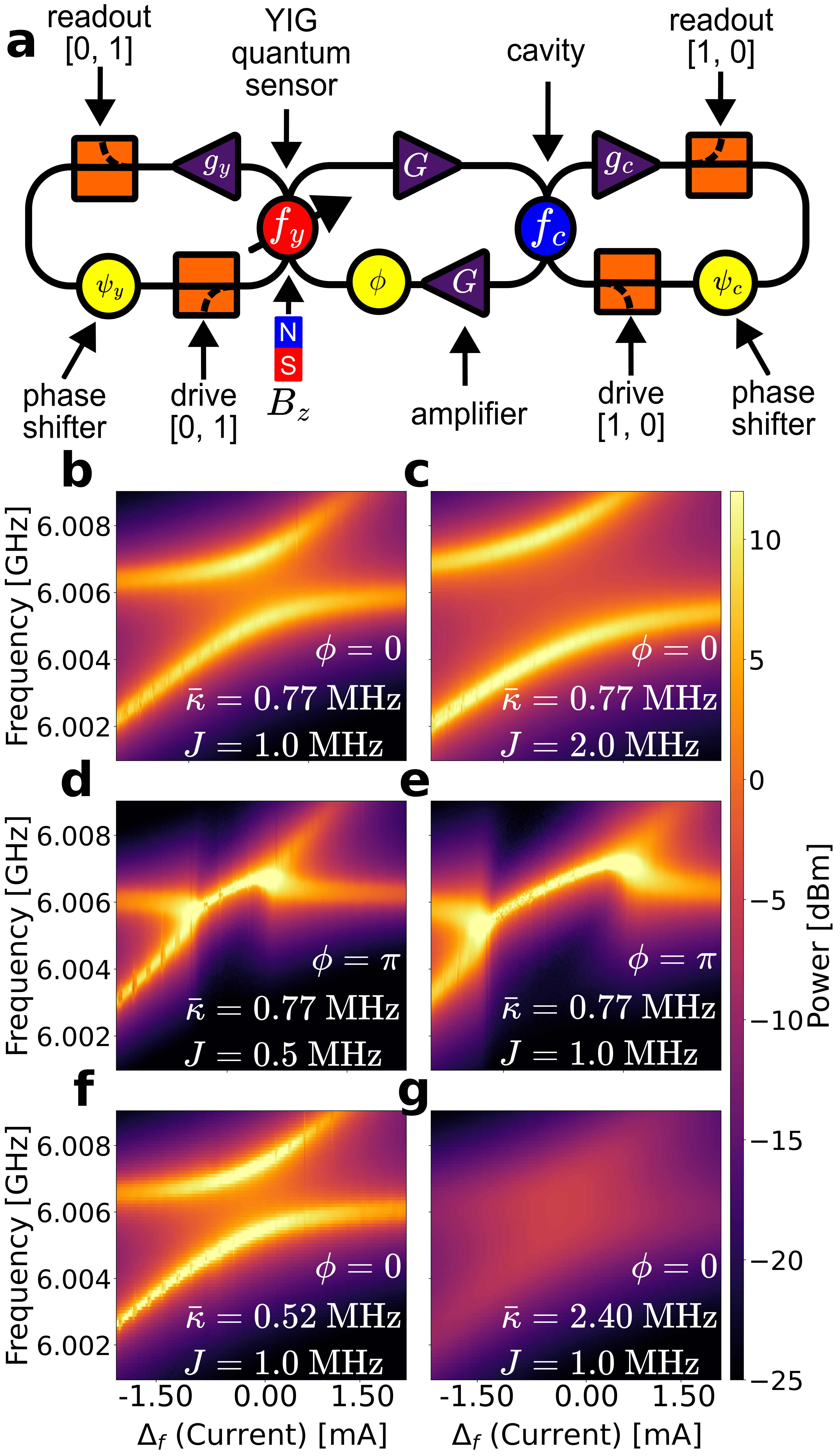
Our experimental architecture is a coupled magnon-photon system, forming a dimer of dissipative harmonic oscillators, each characterized by a resonant frequency and total dissipation rate . The photon mode is the lowest harmonic of a three-dimensional microwave cavity [51], while the magnon mode is realized using a 1 mm YIG sphere. YIG exhibits a narrow ferrimagnetic resonance linewidth and is a widely used material in cavity magnonics [43], making it an ideal candidate for our realization of an independent magnon mode. When biased with a static magnetic field, the electron spins in YIG collectively precess about the field axis, forming a resonance analogous to a ferromagnetic resonance (FMR) (for more details, see Supplementary Information). The Larmor frequency depends linearly on the applied field as , where is the Bohr magneton, consistent with the simplified Kittel formula for a uniformly magnetized sphere [52, 53]. The magnon mode is coupled to using two orthogonal wire bonds that encircle the YIG sphere. Without the YIG, the loops are electromagnetically isolated, preventing power transmission between them. When the YIG is inserted, its spin resonance enables microwave coupling between the input and output loops only at frequencies near the Larmor frequency. Therefore, the oscillator hosting the YIG passes signals around , with a FWHM while attenuating others [54].
The magnon and photon modes are spatially separated by approximately one meter using SMA microwave coaxial lines, as shown in Fig. 1a. By utilizing unidirectional microwave amplifiers, the coupling between the modes can be split into independent coupling paths, each of which consists of a fixed-gain amplifier followed by a digital attenuator, effectively forming a digitally controlled variable-gain amplifier with gain that we use to tune the overall coupling [55]. To ensure symmetric coupling rates, we carefully measure the insertion losses of components on each coupling path and offset the digital attenuators accordingly. The coupling phase introduces phase non-reciprocity in the coupling, which, while not necessarily breaking reciprocity in the strict electromagnetic sense, produces direction-dependent phase evolution, effectively producing a synthetic gauge field [46]. To tune the coupling phase, we insert a digital phase shifter in one of the coupling paths (Fig. 1a). The phase shifter enables continuous tuning of the complex coupling coefficient, , across the full range while preserving the coupling magnitude. We focus on two representative cases: reciprocal phase (RP) coupling () and anti-reciprocal phase (ARP) coupling (). These two phase configurations produce distinct coupling dynamics between the magnon and photon modes, consistent with traditional level repulsion and level attraction [44]. The system exhibits level repulsion for RP coupling, characterized by an avoided crossing whose gap increases with the coupling strength (Fig. 1b,c,f,g). Modifying the average dissipation rate,
| (1) |
changes the linewidths of the hybridized modes while preserving the repulsion behavior (Fig. 1f,g). In contrast, ARP coupling results in level attraction, where the hybridized modes coalesce and split as the individual frequencies are detuned. The extent of the coalescence region increases with (Fig. 1d,e).
To achieve full parameter tunability, each mode is equipped with a self-feedback loop consisting of a phase shifter with phase and an effective variable-gain amplifier with gain (Fig. 1a), where the subscripts correspond to the cavity and YIG self-feedback loops, respectively. Specifically, is controlled using a coarse digital attenuator, while is controlled using both a digital attenuator and an analog attenuator in series, for higher resolution control. and enable tunable constructive and destructive feedback interference, adding additional control over and for each mode. The interactions between and the mode parameters are not explicitly modeled; instead, we utilize to achieve the desired and . At each step during the experiment, we measure and extract fitted values of , and their uncertainties . To achieve this, the dimer includes microwave switches to enable three distinct operating modes: cavity readout, YIG readout, and normal operation. In cavity (YIG) readout operation mode, the magnon-photon coupling is disabled, and transmission is measured through the cavity (YIG) mode in isolation, allowing for measurement of and their associated uncertainties . During normal operation, magnon-photon coupling is enabled, the cavity is driven, and the YIG is measured. Figure 1 illustrates the complete experimental schematic (Fig. 1a and associated transmission measurements in normal operation (Fig. 1b–g), highlighting the independent tunability of all model parameters.
III Theory
One of the core contributions of this work is a unified state-space framework for analyzing EPs and TPDs in dimers. Our state-space model is algebraically equivalent to the standard coupled-mode or quantum-Langevin formalisms at the linear, semiclassical level, yet offers practical advantages for our study. Specifically, a single representation captures both the eigenspectrum that defines EPs and the transmission spectrum that reveals TPDs. The state space model matches all the relevant features in the experimental data: peak locations, TPDs, EPs, and instability transitions. Our theoretical model is motivated by the dissipative Hamiltonian of magnon-photon coupling studied in cavity magnonics, where a coupling phase in one of the off-diagonal elements induces phase non-reciprocity [47]. For completeness, in the Supplementary Information, we motivate this model using an effective quantum Hamiltonian with non-reciprocal hopping between modes and the corresponding semi-classical limit, and recover the state-space matrices .
The dynamics of the dimer are governed by semiclassical equations of motion
| (2) |
where denotes the complex coherent state amplitudes of the photon () and magnon () modes. is the drive vector, where () represents driving the cavity (YIG) with drive strength . Complex mode amplitudes are measured by with the readout vector, () corresponds to reading out the cavity (YIG). The theoretical model in Eq. 2 reproduces relative power between the two modes rather than the absolute microwave power in dBm, which is sufficient for analyzing TPDs, EPs, frequency-peak-splitting, and instability.
In our architecture, are all independently tunable. However, and are controlled with high-resolution analog voltage sources, while and rely on discrete digital control with coarser resolution. Thus, to enable fine-grained experimental sweeps, we fix and , and sweep and . Accordingly, it will be convenient to consider parameter detunings defined by
| (3) | ||||
| (4) |
Utilizing the relative detuning parameters defined in Eqs. 3 and 4, we construct a semi-classical dynamical matrix in the rotating frame of the drive at frequency (see Supplementary Information for derivation)
| (5) |
Although the expression in Eq. 5 includes both relative parameters and absolute parameters , , this representation reduces the complexity of the expressions that follow and reflects a more natural coordinate system for analyzing the dynamical behavior of the system. Furthermore, although we use dimensional parameters here, the theory can also be nondimensionalized by normalizing all parameters by (see Supplementary Information).
Next, we consider the eigenspectrum of , which we use to parameterize EPs in the system. Following that, in Sec. III.0.2, we consider the transmission spectrum, used to parameterize TPDs. Finally, in Sec. III.0.3, we summarize and unify the results of EPs, TPDs, and instability transition locations in the system. The discrepancy between the EP and TPD for the RP configuration [36, 37] and ARP configuration [25] have been explored separately and experimentally validated in previous work. Here, we generalize this analysis to all values of the coupling phase , and present the representative cases and . We extend this to in the Supplementary Information.
III.0.1 Eigenspectrum Analysis
The eigenvalues of in Eq. 5, denoted , encode information about the physical characteristics of the system dynamics. Here, the real part of each eigenvalue corresponds to dissipation () or gain (), and the imaginary part corresponds to the oscillation frequency of the modes. This convention differs from the more typical formulation in coupled-mode theory, where the system Hamiltonian generates dynamics through , leading to the opposite association between real and imaginary parts of the spectrum [56]. Our convention reflects the semiclassical treatment of driven-dissipative systems, consistent with standard practice in input–output theory for non-Hermitian photonics analyzed in state-space form [57, 55].
The eigenvalues can be written as a symmetric pair around a central complex value , with splitting given by , or in terms of the model parameters as
| (6) | ||||
| (7) | ||||
| (8) |
The quantity defines the complex spectral splitting between the eigenvalues, and, remarkably, appears throughout the analysis for EPs, Petermann noise factor, and even TPDs in the form . Since the radicand of Eq. 7 is generally complex, the square root is computed using the principal value, which we can define in polar form as , with the argument . This choice ensures continuity of in parameter space except at branch points along the zero contour . This zero contour is a curve along which the two eigenvalues are degenerate in real and imaginary components. To determine whether these degeneracies are ordinary crossings or EPs, we examine the eigenvector coalescence, quantified by the Petermann noise factor.
The Petermann noise factor is defined as , where and denote the left and right eigenvectors of [28, 7]. For convenience, we use the mean diagonal Petermann noise factor , whose deviation from unity measures eigenvector non-orthogonality and diverges at EPs [58]. While originally formulated to describe excess spontaneous emission in unstable lasers [28], the Petermann noise factor now serves more generally as a predictor of noise enhancement in non-Hermitian systems [27, 59]. For in Eq. 5, the mean diagonal Petermann noise factor is
| (9) |
When , Eq. 9 evaluates to unity for all values of and , yielding purely orthogonal eigenvectors. In this regime, the only possible spectral degeneracies are diabolic points (DPs), which correspond to real-eigenvalue crossings and require to occur. In contrast, introducing nonzero and enables eigenvector non-orthogonality and thus eigenvector coalescence. Equation 9 diverges as , while the numerator remains finite, signaling the presence of an EP. For a given , solving , equivalent to finding where , yields a continuous manifold of EPs in parameter space, called an exceptional surface [60]. This exceptional surface is parameterized by
| (10) |
For our experiments, we analyze two distinct EP configurations along the exceptional surface, namely the reciprocal phase EP (RP-EP) and anti-reciprocal phase EP (ARP-EP), given by
| ARP-EP: | |||
| RP-EP: |
Moreover, the Supplementary Information explores a hybrid EP at , where the coupling is truly non-reciprocal.
III.0.2 Transmission Spectrum Analysis
Equation 2 governs the time dynamics of the driven two-mode system, with a general solution given by for time-independent drive and nonsingular . During experiments, we perform a homodyne readout of the transmission signal, which captures the steady-state mode amplitudes after transient dynamics have ceased. To model this behavior, we set in Eq. 2 and solve for the steady-state response with
| (11) | |||||
| (12) |
where is proportional to the detected power. Equation 11 is only valid when the system is stable, given by the Hurwitz stability criterion, which requires all real parts of the eigenvalues to be negative. When becomes unstable, the dynamics are eventually stabilized by saturation of amplifiers, leading to nonlinear phenomena, characterized in previous work but not considered here [55] (See Supplementary Information for details). Transmission peak frequencies correspond to the critical points of , obtained by solving for . This condition yields a nonlinear equation for , which can be expressed as a depressed cubic in terms of an auxiliary variable of the form
| (13) | ||||
| (14) | ||||
| (15) |
The three roots of Eq. 13 are the critical points of and, remarkably, are related to the eigenspectrum of in Eq. 5 through in Eq. 7.
When Eq. 13 admits three real roots, the outermost roots (the largest and smallest), denoted , are used to find the transmission peak locations, while the intermediate root, denoted , is used to find the local minimum between the two peaks. When there is no splitting, Eq. 13 admits one real root, denoted , corresponding to the single peak frequency. Solving Eq. 13 for a closed form solution of the roots in terms of can either be done using Cardano’s method, which involves square and cube roots, or through a trigonometric solution first posed by François Viète in 1615 [61, 62, 63], which yields a solution for as
| (16) | ||||
| (17) |
and a solution for given by
| (18) |
The expression for the splitting between the two peaks, , admits a compact expression in terms of in Eq. 17 as
| (19) |
Equations 16 and 19 are undefined at , and are otherwise only valid in regions where the discriminant, expressed algebraically as
| (20) |
is positive, signifying three real root solutions to Eq. 13. In contrast, when , Eq. 16 and 19 are invalid, as there is only one real root, , given by
| (21) |
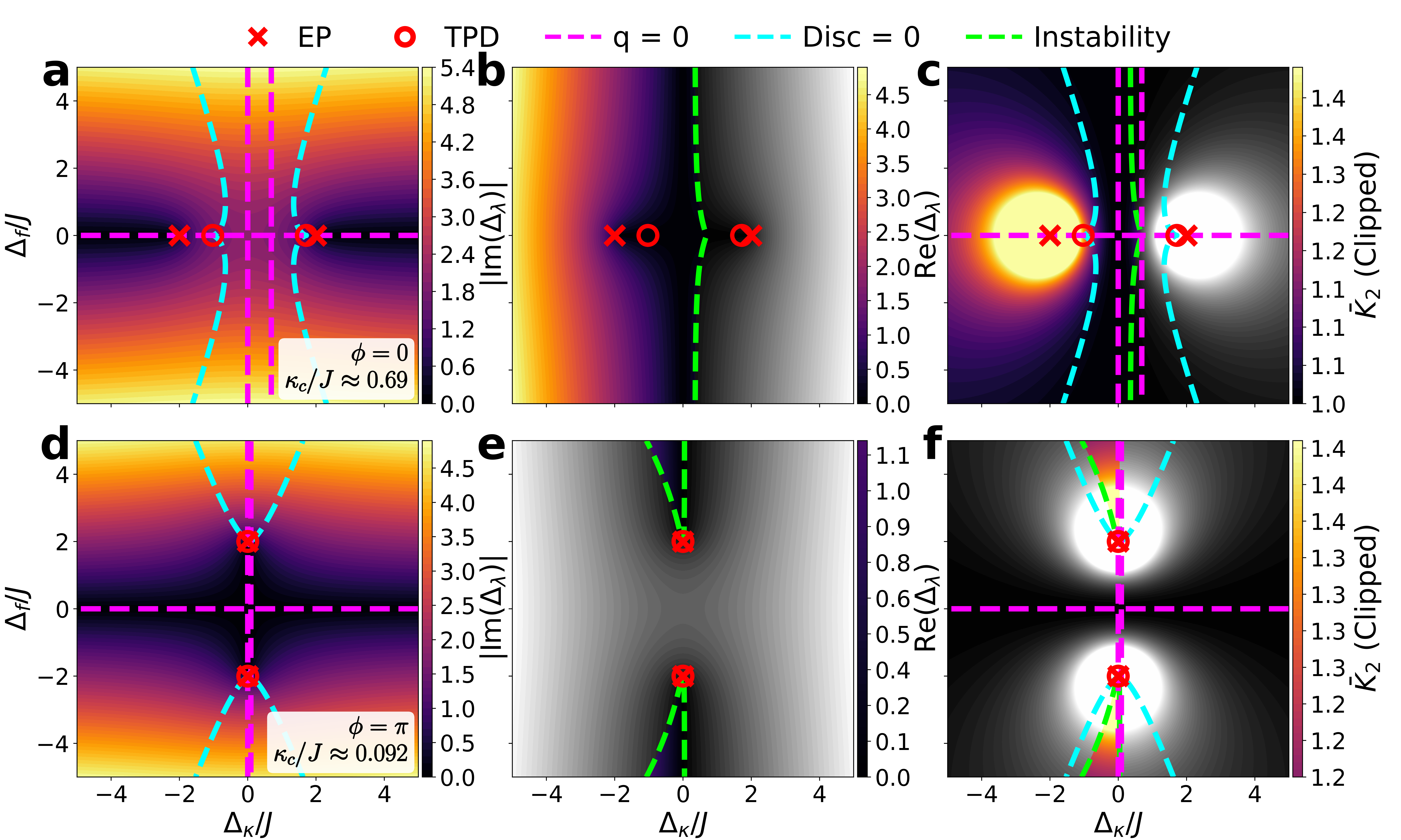
Naturally, the condition marks the boundary between the single-peak and split-peak regimes. This boundary can be represented as a zero-contour in - space, plotted in Fig. 2a, d. However, alone does not define the locations of TPDs, as it is not guaranteed that at . This can be illuminated through the geometric representation of the discriminant
| (22) |
where are the roots of Eq. 13. For , one of the roots is real, given by , and the other two roots are a complex conjugate pair, not considered here. For , are respectively. Finally, at , a multi-root degeneracy occurs, corresponding to the coalescence of either or with the central root , but not necessarily all three required for a TPD.
To differentiate between causing a double-root degeneracy or a true TPD, an additional condition is required. In Eq. 20, enforcing and causes as well. Then, simplifies Eq. 13 to , a triple degeneracy. Thus, TPDs occur precisely at intersections of the zero contours defined by and , which are plotted in Fig. 2. The zero contour is the sensor optimal path and is plotted in Fig. 2a,c,d,f. The optimal path () is the parameterized curve treated as the independent variable during experimental operation, and is () for the RP (ARP) configuration. In the Supplementary Information, we comment on how this relates to choosing a TPD based on the type of sensor being built and the added complexity of TPDs, where the optimal paths become curved contours requiring precise, simultaneous control of and .
III.0.3 Unifying EPs, TPDs, and Instability
To make a concrete connection between the theoretical treatment in the previous section and our experimental results, we begin by converting the roots, to frequencies observed experimentally using
| (23) |
where we can see, naturally, that .
To unify EPs and TPDs, we first consider the cases where TPDs appear exactly at EPs. For the RP configuration, the condition forms a TPD-EP pair with balanced loss and gain, with locally around the TPD. For the ARP configuration, the condition forms TPD-EP pairs at , with globally. A geometric interpretation of the correspondence between peak locations and imaginary eigenvalues is presented in the Supplementary Information. Next, we generalize the correspondence between TPDs, , EPs, and , to the cases where both modes are dissipative (). In this more typical scenario, the peak locations are distinct from the imaginary eigenvalues, and the TPDs shift in parameter space away from the EPs with .
The locations of EPs and TPDs, along with contours for splitting and instability thresholds, are visualized for a specific ratio in Fig. 2a, b, d, e for the RP configuration ()(Fig.2a, b, c) and the ARP configuration ()(Fig.2d, e, f). In the ARP configuration, the EP occurs at , while the TPD occurs at (Fig. 2d). The system becomes unstable and nonlinear at , provided (Fig. 2e). The instability transition is determined using the condition . In the RP configuration, the RP-EP lies at , but the RP-TPDs occur at , provided (Fig. 2d). The TPD can be displaced from the EP in parameter space, significantly reducing the Petermann noise factor at the RP-TPD (Fig. 2c), compared to the ARP-TPD in Fig. 2f. The instability transition occurs at for , and for . Ultimately, this separation between the EPs and TPDs is crucial for interpreting the experimental data in Fig. 3 and understanding the functional role of EPs versus TPDs in sensor applications.
IV Results
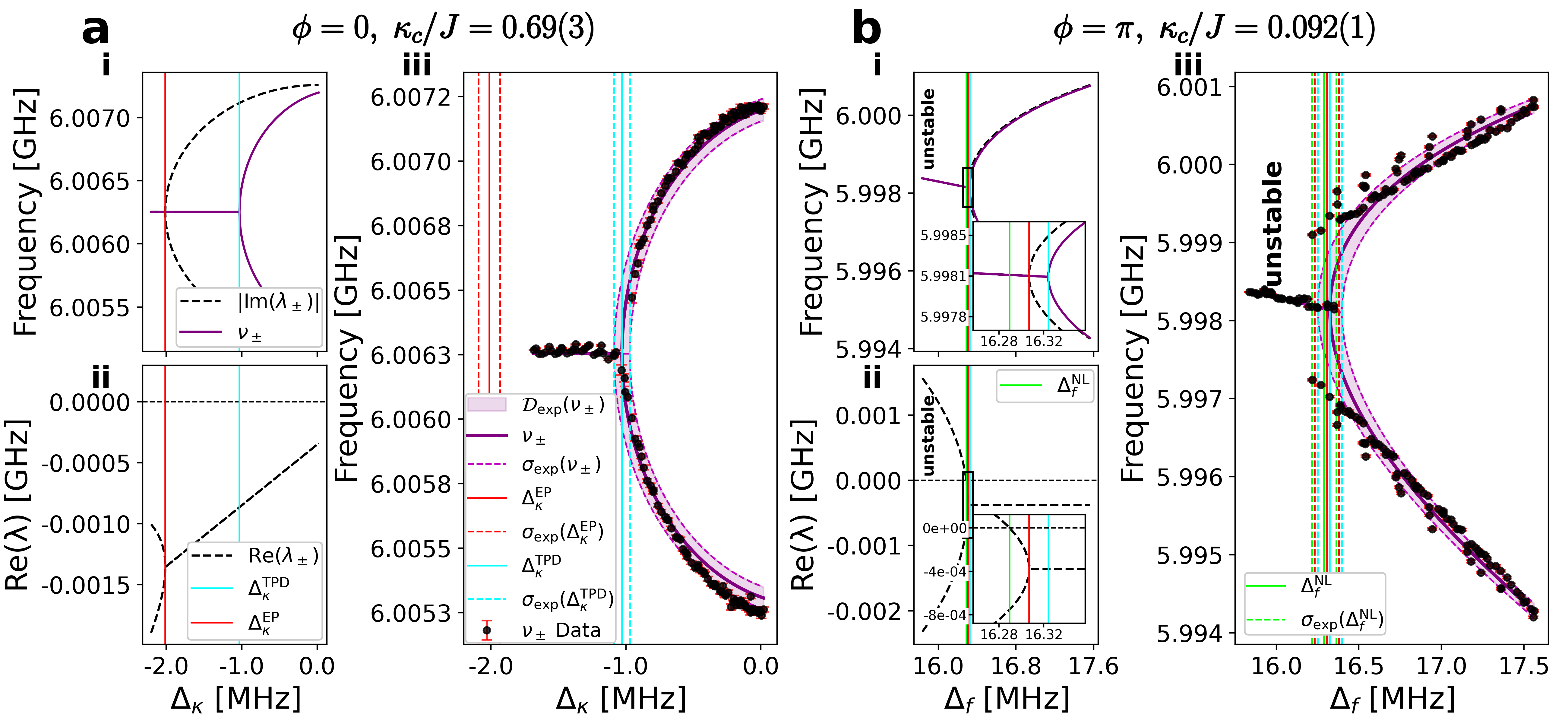
Here, we report experimental data for both RP and ARP configurations, selecting deliberately disparate values of to highlight the contrasting behavior between TPDs that lie close to or far from their corresponding EPs. To ensure the validity of our linear model, we select TPDs that involve purely dissipative dynamics. For the RP configuration, we select a representative small value of MHz with MHz, yielding a ratio . As shown in Fig. 2c, this choice of RP-TPD is significantly displaced from the RP-EP. For the ARP configuration, we select a representative large value of MHz, with MHz. This choice of places the TPD, EP, and instability transition within a 50 kHz window (Fig. 2f).
The experimental methods are summarized here, and detailed in Methods. For each value of () for the RP (ARP) configuration sweep, we independently probe each mode in isolation (by setting ) using the microwave switch technique described in Sec. II and fit the isolated mode trace to a Lorentzian to extract cavity (YIG) parameters and the associated fit uncertainties . In general, refers to uncertainty extracted from least squares regression covariance matrix. Then, coupling is activated (), and the coupled transmission Eq. 12 is fit to the experimental data using , extracting and for each data point. Finally, are fit to Eq. 23 to extract data, reported in Fig. 3iii, with error bars, representing uncertainty propagation from (See Methods).
The fit values of and are extracted for all data points, and averaged across the entire experiment, denoted as . We also quantify experimental uncertainty in these parameters, , based on the standard deviation of and across the entire experiment, which is distinct from fit uncertainty, , extracted for each data point individually. Then, are used to simulate a distribution of possible , denoted (shaded regions in Fig. 3iii), with standard deviation . Finally, are used to report , , , while determine , , and .
IV.0.1 Reciprocal Phase Configuration
To probe the RP-TPD, we set the coupling phase to and the coupling strength to . The YIG () and cavity () frequencies are held constant at GHz such that , and the dissipation rates and are initialized to such that . We sweep from to using a voltage-controlled attenuator on the YIG self-feedback loop. As is tuned, the dissipation detuning approaches the RP-TPD at , at which point the split peaks coalesce to a single peak. For the RP configuration, the RP-EP is significantly displaced from the RP-TPD, occurring at , outside the range of the experimental scan (see Methods). Furthermore, precise control of allows the condition to be achieved throughout the entire experiment using a digital proportional controller. Overall, the displacement of our representative RP-TPD from the RP-EP, which reduces Petermann factor noise at the RP-TPD, along with careful stabilization of , provides a strong fit of the data and theory.
IV.0.2 Anti-Reciprocal Phase Configuration
In the ARP configuration, we seek to consider the case where the TPD is near the EP. To do this, we set the coupling configuration to and select MHz with MHz such that . We sweep the YIG frequency from to GHz by varying the current through an external electromagnet, controlling . As the YIG frequency is tuned, the detuning approaches the ARP-TPD at MHz, when the peaks merge. Crucially, for this choice of and , the instability transition is also near the ARP-TPD. When enters the uncertainty bounds of MHz, given by MHz [dashed lime lines in Fig. 3f], the experimental data deviate from the model, likely due to the impending nonlinearity that arises in the unstable regime. Furthermore, the proximity of the ARP-EP, at MHz to the ARP-TPD causes the Petermann noise factor at the ARP-TPD to be nearly divergent. Overall, the proximity of the ARP-TPD to the ARP-EP and instability transition introduce significant deviations between the theory model and the experimental data.
IV.0.3 Performance Metrics of TPDs
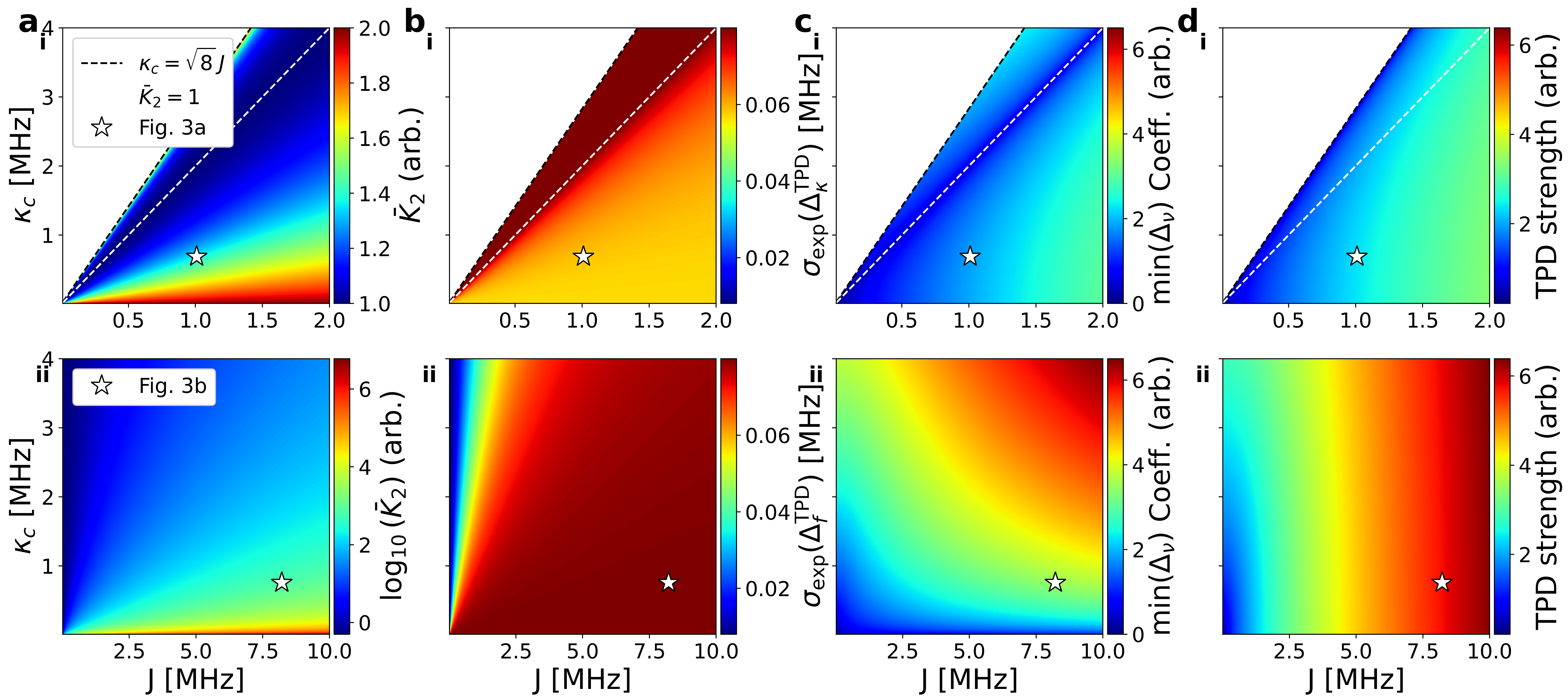
A critical implication of separating TPDs and EPs is that TPDs can be moved around in parameter space using , while the EP locations are not affected by (see geometric intuition in the Supplementary Information). We have shown in Fig. 2c, f that the proximity of TPDs to EPs, controllable with , changes the Petermann noise factor at the TPD and may attribute to the quality of data in 3iii. However, although the Petermann noise factor is one component of heightened uncertainty around EPs, it is not the only consideration. Here, we analyze other robustness and performance metrics associated with TPDs, and show that while the Petermann noise factor can be suppressed by shifting a TPD away from the EP, other forms of errors that are dependent on and are also relevant, and do not generally follow the same parameter dependence as the Petermann noise factor. In Fig. 4, we depict the Petermann noise factor, , as a function of and , as well as novel metrics for TPD performance: TPD splitting strength, TPD location uncertainty propagation, and TPD minimum resolvable peak splitting, which we define in Sec. IV.0.4-IV.0.6 sections.
IV.0.4 TPD Location Uncertainty
Practical sensor operation requires accurate knowledge of or , both depending on and . Importantly, uncertainty in these parameters, , propagates to . Furthermore, we emphasize that at the TPD, . This result is critical because cannot be calculated using standard uncertainty propagation techniques, as is non-differentiable at the TPD. This correspondence between and can be seen in the shaded region in Fig.3iii that encapsulates the experimental data. The first order propagation of uncertainty for the TPD locations is given by
| (24) |
We stress that Eq. 24 is itself dependent on the values of and (see Supplementary Information). Thus, with constant , uncertainty propagation to could be minimized by judiciously selecting and . Panels depicting TPD location uncertainty propagation for the RP (ARP) configurations are included in Fig. 4b.i(ii).
IV.0.5 TPD Splitting Strength
The concept of splitting strength was initially introduced for EP-based sensors in Ref. [64] to quantify the pre-factor of the square root splitting with respect to the perturbation being measured. Specifically, near an EP, the splitting of imaginary eigenvalues follows , where denotes the perturbation strength and is the splitting strength. Recent work has extended this concept to the ARP-TPD [25]. Here, we extend this concept to other TPDs by analyzing the coefficient of the square root term of the Puiseux series expansion of around the TPD, with respect to , a perturbation which is a function of () for the RP (ARP) configuration. The expansion yields the best approximation of in the proximity of each TPD for sufficiently small , where is the strength. We find that this strength coefficient can be expressed as
IV.0.6 Minimum Resolvable Peak Splitting
The observant reader will notice that the split peaks of the experimental data in Fig. 3iii have an abrupt jump near the TPD, indicating that fails to smoothly approach zero at the TPD itself. We refer to this effect as , which is arguably the most destructive model error for sensor performance. To understand for true TPDs versus imperfect TPDs, we begin by recalling that a true TPD is a triple-degenerate root in the cubic equation defined in Eq. 13 and requires crossing along the path , which is () for the RP-TPD (ARP-TPD). Satisfying this stringent requirement causes the peak splitting to be precisely at the TPD, expressed as . However, in any experimental apparatus, this is a challenging task. Here, we consider what happens to in the case of deviation from the path, a manifestation of TPD parameter hypersensitivity.
If the contour is crossed with a path in parameter space where , peak splitting will still occur, but not with a continuous square root profile. Instead, the splitting is zero until it jumps to , increasing from there with a profile much closer to linear splitting than square root splitting. Mathematically, crossing with is only a double degeneracy, with two repeated roots, denoted while one root remains a simple, separated root . We quantify the distance between these roots as the minimum resolvable splitting, which equates to zero for a triple degeneracy (a true TPD). For the depressed cubic defined in Eq. 13, the same François Viète returns with formulas that relate the coefficients of the polynomial to sums and products of its roots. We use the Viète equations to relate , solving . We find that the minimum splitting can be expressed in terms of as
| (27) |
Thus, the inability to resolve square root splitting with respect to the sensing parameter grows with the cube root of . To quantify the notion of strength of this error, is expressed as a function of () for the RP-TPD (ARP-TPD), then approximated as the first (cubic order) term of the Puiseux expansion of for the two TPDs, isolating the response as a function of or . This coefficient is expressed as
| (28) | ||||
| (29) |
Panels depicting the coefficient for the two TPDs are included in Fig. 4c, g.
The performance metrics introduced in this section can be used as a guide to optimize TPD-based sensors. For example, the RP-TPD can be placed along a line where , minimizing the Petermann noise factor and coefficient while increasing model uncertainty propagation. For the ARP-TPD, and TPD strength can be increased by moving the ARP-TPD closer to the ARP-EP, which drastically increases the Petermann noise factor. Ultimately, the design of TPD-based sensors must balance competing metrics based on the constraints and goals of the specific experimental platform.
V Discussion and Outlook
This work presents a highly tunable experimental platform and a unified theoretical framework for systematically investigating EPs and TPDs in coupled oscillator systems. A synthetic gauge field is engineered through the complex coupling term , effectively unifying previously distinct two-dimensional configurations of EPs and TPDs into an exceptional surface. This synthetic gauge field enables continuous tuning between RP and ARP coupling regimes, and we report the distinct properties of the RP-EP, RP-TPD, ARP-EP, and ARP-TPD, highlighting their differences through experimental and theoretical analysis.
Our magnon-photon platform offers practical pathways towards implementing new TPD-based sensors. Specifically, by including the magnon mode, our system allows for direct observation of external magnetic fields through the frequency detuning in the ARP configuration, or external electric fields that modify the analog attenuator, adjusting and thus dissipation detuning in the RP configuration. In this work, we focus on demonstrating the broad tunability of our architecture, but future research can leverage this platform to engineer robust and optimized sensors that likely have less tunability to avoid parameter hypersensivity issues.
Our theoretical framework separately considers the EPs and TPDs in parameter space. We show that the TPDs do not generally occur at the EPs and provide a mathematical framework to differentiate between the location of all EPs, TPDs, and instability transitions. Remarkably, EPs and TPDs can be characterized using the eigenvalues of the dynamical system matrix through and . Furthermore, we solidify the role of and as control parameters, which can be used to deliberately place TPDs to positions where the eigenbasis remains complete or even orthogonal, reducing the inherent noise enhancement through the diverging Petermann noise factor. Finally, we present new performance metrics for TPDs using and based on their splitting strength and robustness to model errors, facilitating informed optimization of sensor designs.
The framework and methods developed in this study may extend beyond semi-classical dimers. For example, our system naturally lends itself to studying nonlinear phenomena associated with EPs and TPDs, due to the active gain elements that saturate in the unstable regime. The mathematical tools and experimental methods demonstrated here may be generalized to higher-dimensional lattices and more complex resonators and oscillator networks, potentially revealing new spectral phenomena, topological behaviors, higher-dimensional exceptional surfaces, and EPs [38] or even higher-order TPDs. We leave these exciting steps to future work.
VI Methods
VI.1 Device Description
Our setup includes a vector network analyzer (Quantum Machines OPX+ Quantum Controller) and a local oscillator (SignalCore SC5511A) for collecting the data displayed in Fig 1, 3. Our apparatus consists of a custom-built microwave cavity with mechanically tunable frequency and output-port coupling rates and a custom-built oscillator realized from a 1 mm diameter YIG sphere, placed on top of a co-planar waveguide (Minicircuits CMA-83LN+). The YIG sphere is coupled to the ground using orthogonal wire bonds. Magnon and photon modes are coupled over a meter-scale distance using flexible SMA wires (Minicircuits 086-11SM+). To achieve variable gain amplification and tunable coupling, we place a fixed-gain amplifier (Minicircuits CMA-83LN+), directly followed by a digital attenuator (Vaunix LDA-5018V), and tune the attenuation digitally using the Vaunix Python API. A digital phase shifter (Vaunix LPS-802) modifies the phase for hopping between the cavity and YIG.
We use three digital switches to probe each mode individually during experimental operation without modifying the apparatus. Two Vaunix LSW-802P4T switches (1-input, 4-output) are used on the drive and readout lines to select which mode is being driven or read out. A 1-input, 2-output (Vaunix LSW-802PDT) switch is included on one of the coupling wires to disable or enable coupling when probing each mode individually. When disabled, the signal is routed directly to a 50- terminator to ensure impedance matching and reduce reflections. Directional couplers (Minicircuits ZADC-13-73-S+) drive and read out each mode, attaching to the self-feedback loops.
Experimental control of parameters is achieved through a Python API. is primarily tuned using an external magnetic field controlled by an electromagnet driven by a digital current source (SRS CS580). We offset the frequency of the YIG to 6 GHz using a fixed neodymium magnet and tune using the current source. To modify with high resolution, we insert an analog voltage-controlled attenautor (Analog Devices HMC812ALC4 integrated with EV1 eval board) on the YIG self-feedback loop, and modify the voltage using precision voltage source (SRS DC205). A full schematic diagram including all components and wiring is included in the Supplementary Information.
VI.2 Parameter Calibration
During an experimental sweep, all the parameters are necessary for data analysis. Parameters are measured during each step of the independent variable, using the RF-switch-based probing method described in Sec. VI.1. We use the experimental apparatus to set and , then couple the two modes together and change the digital phase shifter until the hybridized peaks are the same height in transmission, which defines the phase origin, . Finally, is a fitted parameter, extracted from fitting (see Supplementary Information) to each trace of the hybridized data.
VI.3 Experimental Nonidealities
Although the experimental platform enables precise control over key parameters, residual experimental uncertainties persist. For instance, we have observed that modifications of phases can result in changes to effective loss rates due to interference, effectively creating crosstalk between experimental parameters for each mode. However, since we can separately infer , we can calibrate away any crosstalk between these variables in our system. However, experimental nonidealities cannot be ignored for the RP-TPD experimental sweep, where the voltage-controlled attenuator described in Sec. VI.1 is swept. The voltage-controlled attenuator imparts a significant phase shift while modifying attenuation. This parasitic phase shift causes the YIG frequency to drastically change during the RPEP experimental sweep, deviating from the required path needed to see the RP-TPD. To account for this, we implement a simple digital proportional feedback control system with the current-controlled electromagnet to correct and keep while changing . The effect of this control system is included in the Supplementary Information. Additionally, for the RP configuration, the maximum is limited to before the YIG resonance is indistinguishable from the system noise floor. Thus, this limits the choices of and for experimental scans to ensure that does not breach this maximum threshold before the TPD is reached.
VI.4 Data Analysis
When probing the YIG or cavity individually using the RF-switch-based isolation method, we convert the output data extracted from the OPX+ Quantum Controller into a linear scale and fit the data to a Lorentzian profile. From the fit, we extract , and using the elements of the least squares regression covariance matrix. Then, for data where the coupling is enabled, we fit to the data (see Supplementary Information), fitting and . Then, the equation for is fit to the data using which we report as experimental data in Fig. 3. To quantify the fit uncertainty of , we fit to the data times drawing from a multivariate normal distribution in with uncertainties . For each shot in , we calculate , yielding a distribution with standard deviation . The error bars in Fig. 3 are , a measure of the propagation of uncertainty of the fit parameters to the peak locations of the coupled system.
We also seek to obtain a global uncertainty across the entire experiment, accounting for variations in and across an entire sweep. The average of and across an entire experiment is The experimental standard deviation is . To represent the set of possible values of under experimental uncertainty in , we fit to the data times drawing from a multivariate normal distribution in , with uncertainties . For each shot in , we calculate , yielding a distribution based on experimental parameters with standard deviation Fig. 3(c, f) depicts [purple shaded] for panels Fig. 3iii.
The location of EPs, TPDs, and instability is found using . The experimental uncertainty in and also propagates to the location of EPs, TPDs, and instability. Using first order uncertainty propagation, we find , is found using Eq. 24. is found in the same way, equal to .
Beyond the instability transition, the linear model is no longer valid, and the experimental results are no longer well-described by . We hope to explore the complete nonlinear model that considers amplifier saturation and other nonlinear stabilization effects in future work.
VII Data Availability
The data that support the findings of this study are available upon reasonable request.
VIII Code Availability
The data analysis code will be available online on GitHub.
References
- Ballentine [1998] L. E. Ballentine, Quantum mechanics: a modern development (World Scientific, Singapore ; River Edge, NJ, 1998).
- Bender [2007] C. M. Bender, Reports on Progress in Physics 70, 947 (2007).
- Müller and Rotter [2008] M. Müller and I. Rotter, Journal of Physics A: Mathematical and Theoretical 41, 244018 (2008).
- Latinne et al. [1995] O. Latinne, N. J. Kylstra, M. Dörr, J. Purvis, M. Terao-Dunseath, C. J. Joachain, P. G. Burke, and C. J. Noble, Physical Review Letters 74, 46 (1995), publisher: American Physical Society.
- Cartarius et al. [2007] H. Cartarius, J. Main, and G. Wunner, Physical Review Letters 99, 173003 (2007), publisher: American Physical Society.
- Kato [1995] T. Kato, Perturbation Theory for Linear Operators, Classics in Mathematics, Vol. 132 (Springer, Berlin, Heidelberg, 1995).
- Ashida et al. [2020] Y. Ashida, Z. Gong, and M. Ueda, Advances in Physics 69, 249 (2020), arXiv:2006.01837 [cond-mat].
- Ozdemir et al. [2019] Ş. K. Ozdemir, S. Rotter, F. Nori, and L. Yang, Nature Materials 18, 783 (2019).
- El-Ganainy et al. [2018] R. El-Ganainy, K. G. Makris, M. Khajavikhan, Z. H. Musslimani, S. Rotter, and D. N. Christodoulides, Nature Physics 14, 11 (2018).
- Miri and Alù [2019] M.-A. Miri and A. Alù, Science 363, eaar7709 (2019), publisher: American Association for the Advancement of Science.
- Thomas et al. [2016] R. Thomas, H. Li, F. M. Ellis, and T. Kottos, Physical Review A 94, 043829 (2016), publisher: American Physical Society.
- Wang et al. [2018] J. Wang, H. Y. Dong, Q. Y. Shi, W. Wang, and K. H. Fung, Physical Review B 97, 014428 (2018), publisher: American Physical Society.
- Fruchart et al. [2021] M. Fruchart, R. Hanai, P. B. Littlewood, and V. Vitelli, Nature 592, 363 (2021), publisher: Nature Publishing Group.
- Klauck et al. [2025] F. U. J. Klauck, M. Heinrich, A. Szameit, and T. A. W. Wolterink, Science Advances 11, eadr8275 (2025), publisher: American Association for the Advancement of Science.
- Partanen et al. [2019] M. Partanen, J. Goetz, K. Y. Tan, K. Kohvakka, V. Sevriuk, R. E. Lake, R. Kokkoniemi, J. Ikonen, D. Hazra, A. Mäkinen, E. Hyyppä, L. Grönberg, V. Vesterinen, M. Silveri, and M. Möttönen, Physical Review B 100, 134505 (2019), publisher: American Physical Society.
- Heiss [2012] W. D. Heiss, Journal of Physics A: Mathematical and Theoretical 45, 444016 (2012), publisher: IOP Publishing.
- Klaiman et al. [2008] S. Klaiman, U. Günther, and N. Moiseyev, Physical Review Letters 101, 080402 (2008), publisher: American Physical Society.
- Rüter et al. [2010] C. E. Rüter, K. G. Makris, R. El-Ganainy, D. N. Christodoulides, M. Segev, and D. Kip, Nature Physics 6, 192 (2010), publisher: Nature Publishing Group.
- Kim et al. [2024] C. Kim, X. Lu, D. Kong, N. Chen, Y. Chen, L. K. Oxenløwe, K. Yvind, X. Zhang, L. Yang, M. Pu, and J. Xu, eLight 4, 6 (2024).
- Wang et al. [2024] C. Wang, J. Rao, Z. Chen, K. Zhao, L. Sun, B. Yao, T. Yu, Y.-P. Wang, and W. Lu, Nature Physics 20, 1139 (2024), publisher: Nature Publishing Group.
- Wiersig [2020a] J. Wiersig, Photonics Research 8, 1457 (2020a).
- Wiersig [2016] J. Wiersig, Physical Review A 93, 033809 (2016), publisher: American Physical Society.
- Wiersig [2014] J. Wiersig, Physical Review Letters 112, 203901 (2014), publisher: American Physical Society.
- Park et al. [2020] J.-H. Park, A. Ndao, W. Cai, L. Hsu, A. Kodigala, T. Lepetit, Y.-H. Lo, and B. Kanté, Nature Physics 16, 462 (2020), publisher: Nature Publishing Group.
- Kononchuk et al. [2022] R. Kononchuk, J. Cai, F. Ellis, R. Thevamaran, and T. Kottos, Nature 607, 697 (2022), publisher: Nature Publishing Group.
- Chen et al. [2017] W. Chen, Ş. Kaya Ozdemir, G. Zhao, J. Wiersig, and L. Yang, Nature 548, 192 (2017).
- Wang et al. [2020] H. Wang, Y.-H. Lai, Z. Yuan, M.-G. Suh, and K. Vahala, Nature Communications 11, 1610 (2020), publisher: Nature Publishing Group.
- Siegman [1989] A. E. Siegman, Physical Review A 39, 1264 (1989), publisher: American Physical Society.
- Langbein [2018] W. Langbein, Physical Review A 98, 023805 (2018), arXiv:1801.05750 [physics].
- Soleymani et al. [2022] S. Soleymani, Q. Zhong, M. Mokim, S. Rotter, R. El-Ganainy, and S. K. Ozdemir, Nature Communications 13, 599 (2022).
- Mortensen et al. [2018] N. A. Mortensen, P. a. D. Gonçalves, M. Khajavikhan, D. N. Christodoulides, C. Tserkezis, and C. Wolff, Optica 5, 1342 (2018), publisher: Optica Publishing Group.
- Wiersig [2020b] J. Wiersig, Nature Communications 11, 2454 (2020b), publisher: Nature Publishing Group.
- Grant and Digonnet [2021] M. J. Grant and M. J. F. Digonnet, Optics Letters 46, 2936 (2021), publisher: Optica Publishing Group.
- Loughlin and Sudhir [2024] H. Loughlin and V. Sudhir, Physical Review Letters 132, 243601 (2024).
- Zhang et al. [2019] M. Zhang, W. Sweeney, C. W. Hsu, L. Yang, A. D. Stone, and L. Jiang, Physical Review Letters 123, 180501 (2019), publisher: American Physical Society.
- Geng and Zhu [2021] Q. Geng and K.-D. Zhu, Photonics Research 9, 1645 (2021), publisher: Optica Publishing Group.
- Lu et al. [2025] X. Lu, Y. Yuan, F. Chen, X. Hou, Y. Guo, L. Reindl, Y. Fu, W. Luo, and D. Zhao, Microsystems & Nanoengineering 11, 1 (2025), publisher: Nature Publishing Group.
- Hodaei et al. [2017] H. Hodaei, A. U. Hassan, S. Wittek, H. Garcia-Gracia, R. El-Ganainy, D. N. Christodoulides, and M. Khajavikhan, Nature 548, 187 (2017), publisher: Nature Publishing Group.
- Chen et al. [2018] W. Chen, J. Zhang, B. Peng, S. K. Ozdemir, X. Fan, and L. Yang, Photonics Research 6, A23 (2018), publisher: Optica Publishing Group.
- Dong et al. [2019] Z. Dong, Z. Li, F. Yang, C.-W. Qiu, and J. S. Ho, Nature Electronics 2, 335 (2019), publisher: Nature Publishing Group.
- Zhang et al. [2017] D. Zhang, X.-Q. Luo, Y.-P. Wang, T.-F. Li, and J. Q. You, Nature Communications 8, 1368 (2017), publisher: Nature Publishing Group.
- Zhang and You [2019] G.-Q. Zhang and J. Q. You, Physical Review B 99, 054404 (2019), publisher: American Physical Society.
- Zare Rameshti et al. [2022] B. Zare Rameshti, S. Viola Kusminskiy, J. A. Haigh, K. Usami, D. Lachance-Quirion, Y. Nakamura, C.-M. Hu, H. X. Tang, G. E. W. Bauer, and Y. M. Blanter, Physics Reports Cavity Magnonics, 979, 1 (2022).
- Harder et al. [2018] M. Harder, Y. Yang, B. Yao, C. Yu, J. Rao, Y. Gui, R. Stamps, and C.-M. Hu, Physical Review Letters 121, 137203 (2018).
- Yao et al. [2019] B. Yao, T. Yu, X. Zhang, W. Lu, Y. Gui, C.-M. Hu, and Y. M. Blanter, Physical Review B 100, 214426 (2019), publisher: American Physical Society.
- Gardin et al. [2024] A. Gardin, G. Bourcin, J. Bourhill, V. Vlaminck, C. Person, C. Fumeaux, G. C. Tettamanzi, and V. Castel, Physical Review Applied 21, 064033 (2024), publisher: American Physical Society.
- Wang and Hu [2020] Y.-P. Wang and C.-M. Hu, Journal of Applied Physics 127, 130901 (2020).
- Pang et al. [2024] Z. Pang, B. T. T. Wong, J. Hu, and Y. Yang, Physical Review Letters 132, 043804 (2024), publisher: American Physical Society.
- Hatano and Nelson [1996] N. Hatano and D. R. Nelson, Physical Review Letters 77, 570 (1996), publisher: American Physical Society.
- Wen et al. [2019] R. Wen, C.-L. Zou, X. Zhu, P. Chen, Z. Ou, J. Chen, and W. Zhang, Physical Review Letters 122, 253602 (2019), publisher: American Physical Society.
- Reagor et al. [2016] M. Reagor, W. Pfaff, C. Axline, R. W. Heeres, N. Ofek, K. Sliwa, E. Holland, C. Wang, J. Blumoff, K. Chou, M. J. Hatridge, L. Frunzio, M. H. Devoret, L. Jiang, and R. J. Schoelkopf, Physical Review B 94, 014506 (2016), publisher: American Physical Society.
- Sparks et al. [1961] M. Sparks, R. Loudon, and C. Kittel, Physical Review 122, 791 (1961), publisher: American Physical Society.
- Comstock [1963] R. L. Comstock, Solid State Electronics 6, 392 (1963), aDS Bibcode: 1963SSEle…6..392C.
- Barry et al. [2023] J. F. Barry, R. A. Irion, M. H. Steinecker, D. K. Freeman, J. J. Kedziora, R. G. Wilcox, and D. A. Braje, Physical Review Applied 19, 044044 (2023).
- Salcedo-Gallo et al. [2025] J. S. Salcedo-Gallo, M. Burgelman, V. P. Flynn, A. S. Carney, M. Hamdan, T. Gerg, D. C. Smallwood, L. Viola, and M. Fitzpatrick, Demonstration of a tunable non-hermitian nonlinear microwave dimer (2025), arXiv:2503.13364 [quant-ph] .
- Wang et al. [2023] C. Wang, Z. Fu, W. Mao, J. Qie, A. D. Stone, and L. Yang, Advances in Optics and Photonics 15, 442 (2023), publisher: Optica Publishing Group.
- Steck [2007] D. A. Steck, Quantum and Atom Optics (Oregon Center for Optics and Department of Physics, University of Oregon, 2007) available online: http://steck.us/teaching.
- Zheng et al. [2010] M. C. Zheng, D. N. Christodoulides, R. Fleischmann, and T. Kottos, Physical Review A 82, 010103 (2010), publisher: American Physical Society.
- Ghosh et al. [2024] S. Ghosh, A. Roy, S. Dey, B. P. Pal, and S. Ghosh, JOSA B 41, 2534 (2024), publisher: Optica Publishing Group.
- Zhou et al. [2019] H. Zhou, J. Y. Lee, S. Liu, and B. Zhen, Optica 6, 190 (2019), publisher: Optica Publishing Group.
- Nickalls [2006] R. W. D. Nickalls, The Mathematical Gazette 90, 203 (2006).
- Holmes [2002] G. C. Holmes, The Mathematical Gazette 86, 473 (2002).
- Viète [1615] F. Viète, Opera mathematica volume 4 (1615).
- Wiersig [2018] J. Wiersig, in Parity-time Symmetry and Its Applications, edited by D. Christodoulides and J. Yang (Springer, Singapore, 2018) pp. 155–184.
Acknowledgements.
We thank Joe Poissant for his exceptional support in designing and fabricating the 3D microwave cavities. We thank Lorenza Viola, Michiel Burgelman, and Vincent P. Flynn for their contributions to the foundational work upon which this study builds and for valuable discussions about EPs. We thank Hailey A. Mullen and Tian Xia for valuable discussions. We also thank Dr. Mukund Vengalattore for the valuable guidance and support of the project. Startup funds from the Thayer School of Engineering, Dartmouth College, supported this work. We gratefully acknowledge support from the DARPA Young Faculty Award No. D23AP00192, and from the NSF through Grant DGE-2125733. The views and conclusions in this manuscript are those of the authors. They should not be interpreted as representing the official policies, expressed or implied, of DARPA, NSF, or the US Government. The US Government is authorized to reproduce and distribute reprints for Government purposes, notwithstanding any copyright notation herein.IX Author Contributions
A.S.C., J.S.S.G., and M.F. conceived and designed the experiments, while A.S.C. performed the final set of experiments and calibrations. The theoretical model was conceived by A.S.C. and M.F., and formalized and presented by A.S.C., with S.B. developing and presenting the motivation and derivation of the dynamical matrix. A.S.C. collected, managed, and analyzed data, while generating numerical and analytical simulations, receiving feedback from M.F. All authors jointly validated the results. A.S.C. wrote the manuscript, with copious edits and suggestions from M.F. and edits from J.S.S.G. S.B provided edits and contributed to the introduction, literature review, and supplementary information. M.F. conceived of and supervised the project.
X Competing Interests
The authors declare no competing interests.
XI Additional information
XI.1 Supplementary Information
In this preprint version, the Main Manuscript and Supplementary Information are provided as a single file for immediate access.
XI.2 Correspondence and Request for Materials
Correspondence and material requests should be directed to Mattias Fitzpatrick (mattias.w.fitzpatrick@dartmouth.edu) and Alexander S. Carney (alexander.s.carney.th@dartmouth.edu), respectively. Data supporting the findings of this study are available from the corresponding author upon reasonable request.