Can repeating and non-repeating FRBs be drawn from the same population?

Abstract

Do all Fast Radio Burst (FRB) sources repeat? We present evidence that FRB sources follow a Zipf-like distribution, in which the number density of sources is approximately inversely proportional to their burst rate above a fixed energy threshold—even though both the burst rate and number density span many orders of magnitude individually. We introduce a model-independent framework that predicts the distribution of observed fluences and distances, and repetition rates of an FRB population based on an assumed burst rate distribution per source. Using parameters derived directly from observations, this framework simultaneously explains several key features of the FRB population: (i) The observed ratio of repeaters to apparent non-repeaters; (ii) The much lower ratio of apparent non-repeaters to the total number of Soft Gamma Repeater (SGR) sources within the observable Universe; And (iii) the slightly smaller average distances of known repeaters compared to non-repeaters. We further explore how survey parameters, such as radio sensitivity and observation time, influence these statistics. Notably, we find that the fraction of repeaters rises only mildly with improved sensitivity or longer exposure. This weak dependence could be misinterpreted as evidence that not all FRBs repeat. Overall, our results support the idea that a single population—likely magnetars—can account for the full observed diversity of FRB activity, from very inactive FRB sources like SGR 1935+2154 to the most active repeaters.

1 Introduction

Fast radio bursts (FRBs) exhibit a striking diversity in their observable properties. The isotropic-equivalent energies of extragalactic FRBs with known redshifts span over nine orders of magnitude - from as low as $\sim 6\times 10^{23}\mbox{erg Hz}^{-1}$ in FRB 20200120E (Nimmo et al., 2023) to as high as $\gtrsim 6\times 10^{32}\mbox{erg Hz}^{-1}$ in FRB 20220610A (Ryder et al., 2023). Even individual repeaters can show large variability: for example, bursts from FRB 20201124A cover about five orders of magnitude in energy (Zhang et al., 2022; Kumar et al., 2022). FRB sources also differ greatly in their apparent activity rate (Margalit et al., 2020). Some, like FRBs 20121102A and 20201124A, have been observed to emit dozens of bursts in a single hour (Li et al., 2021; Zhang et al., 2022) while others - such as the Galactic magnetar SGR 1935+2154 - have only produced a single energetic burst with in an observed period of over several years. As discussed in §3, this contrast becomes even more pronounced when comparing sources at similar energies, due to the steep energy dependence of burst rates. A third axis of variation is the inferred number density of sources. For instance, Lu et al. (2022) showed that the volumetric density of highly active extragalactic FRBs like 20180916B and 20121102A is orders of magnitude lower than that of low-activity sources such as SGR 1935+2154 or FRB 20200120E in the nearby M81 galaxy. Given these dramatic differences - in energy output, repetition rate, and source density - it remains an open question whether all FRBs can be unified under a single physical framework, and if so, what underlying parameters account for their apparent diversity.

Perhaps the most striking of the apparent dichotomies, is the observational separation between sources seen only once thus far (“non-repeaters") and those seen multiple times (“repeaters"). The most reliable way to estimate the intrinsic fraction of repeating sources is to consider a blind survey mission such as CHIME. In the first 20 months of its operation, CHIME detected 46 repeating sources (and 14 more candidates), consisting a fraction of $2.6_{-2.6}^{+2.9}\%$ of sources in their sample (Chime/Frb Collaboration et al., 2023). The lack of bimodality in burst rates per source between the population of repeaters and (as of yet) non-repeaters detected by CHIME (with observed rates varying continuously from a few per hour to $\lesssim 10^{-3}\mbox{ hr}^{-1}$), suggests all FRB sources might repeat, and that the low observed fraction is just a reflection of the current sensitivity. The finding that repeaters in this sample have, on average, slightly lower extragalactic DMs than non-repeaters ($\sim 4300\mbox{ pc cm}^{-3}$ as compared with $\sim 600\mbox{ pc cm}^{-3}$), could simply be a selection effect - repeaters are by the nature of their identified repetition, likely to be slightly closer than non-repeaters. This does not require intrinsically distinct populations. Similarly, while there are some small differences between repeater and non-repeater host galaxies (the former being slightly less massive, and having lower metalicity, Sharma et al. 2024), these differences are not statistically meaningful and might in addition be subject to further selection biases.

A less trivial difference between repeaters and non-repeaters is with regards to their spectro-temporal properties. Scholz et al. (2017); Fonseca et al. (2020); Pleunis et al. (2021) have found that FRBs from repeaters are longer in duration and spectrally narrower than non-repeaters. As shown by Metzger et al. (2022), such an apparent bi-modality can be a natural consequence of variation in a single intrinsic parameter, controlling the rate of central frequency drift. When the drift is slow, bursts maintain their intrinsically narrow (time-resolved) spectrum and remain within the detector band for longer. Alternatively, when the drift is fast, the peak frequency sweeps so quickly, that the bursts are temporally unresolved, and their spectra integrated over one temporal bin of the detector appear as wide power laws (PLs). The origin of the frequency drift rate, might have a geometrical explanation, whereby active repeaters are magnetars with the spin, magnetic and line of sight directions all roughly aligned and non-repeaters are preferentially misaligned sources (Beniamini & Kumar, 2025). This interpretation can also help explain the discrepancies mentioned above regarding apparent activity rates and source densities.

A different way to asses the possibility of a shared origin of repeaters and non-repeaters, is to monitor over a long time known, highly active, repeater sources. The energy distribution per source is found (at least by some studies) to be consistent with the energy distribution of non-repeaters (Wang & Yu, 2017; Zhang et al., 2021). Kirsten et al. (2024) have observed FRB 20201124A for over 2000 hours, using 25-32 m class telescopes. They have found that the slope of the burst energy distribution varies both as a function of time (sporadically) and energy (becoming shallower at higher energies). The higher energy slope is consistent with that of non-repeating sources and the time variation helps explain the apparent large range of repeating rates between sources. Similar results (utilizing 1500 hours of observations) were found for another repeater, FRB 20220912A (Ould-Boukattine et al., 2024).

In this paper, we set out to explore whether the activity rates, source densities, and energies of FRB repeaters / non-repeaters can originate from the same underlying population. Our approach is primarily analytic (backed by numerical calculations) and is independent of the nature of FRB sources. We begin, in §2 by exploring the simplest hypothesis supporting a unified FRB origin: that there is a single source type powering all observed FRBs. Then, in §3 (and §B) we expand the model to allow for variable intrinsic rates and typical burst energies. The results are then compared with observations in §4 and implications for magnetar sources are discussed in §5. We conclude in §6.

2 Single source rate

Consider a single population of FRB progenitors, with a volumetric source density $n_{\rm src}$ and an energy dependent rate of bursts per source ,

$$\mathcal{R}(>E_{\nu})=\mathcal{R}_{\rm 0,*}(E_{\nu}/E_{\rm*})^{1-\gamma}$$ (1)

for $E_{\rm min}<E_{\nu}<E_{\rm c}$ and $\gamma>1$, where $E_{\nu}$ is the energy per unit frequency. $E_{*}$ is the energy used for the normalization of the rate per source. Throughout the majority of this work we choose $E_{\rm*}=E_{\rm c}$ (an exception to this is discussed in §B).

At the simplest level, a large sky FRB survey can be described by its limiting (spectral) fluence $\Phi_{\rm lim}$ and by the time, $T$, it spends observing each point on the sky . While lower energy bursts are more common per source (Eq. 1), such bursts cannot be detected to large distances by a fluence-limited survey. At the same time the number of sources increases rapidly with distance. The result is a competition between the detectability of low energy and close-by sources and high energy far-away sources. As detailed below (see also Lu & Piro 2019), for $\gamma<2.5$ the competition is won by the far-away sources. That is, most detected bursts are from large cosmological distances. However, as we describe next, this conclusion does not necessarily hold for active repeaters. This is because, if a single burst energy / distance dominates the entire sample, then this corresponds to a single mean number of repetitions per source during the observed period, $\lambda_{E_{\nu}}=\mathcal{R}(>E_{\nu})T$. Assuming Poisson statistics, the probability that a source will repeat $k$ times during $T$ is $P(k)=\lambda^{k}e^{-\lambda}/k!$ . Therefore, $\lambda/2$ is approximately the ratio between repeaters (sources observed at least twice) and non-repeaters and calibration with the observed ratio leads to $\lambda\approx 0.05$. $P(k)$ becomes vanishingly small for large $k$. For example $P(k\geq 10)/P(k\geq 1)\approx\lambda^{10}/10!\sim 4\times 10^{-20}$. The fact that CHIME has detected multiple sources with more than 10 repetitions clearly means that such a picture is too simplistic and that the distance and / or intrinsic rate per source must be varying for sources detected multiple times. The first point is addressed below and the second in §3.

We define $r_{z}$ as the proper distance up to $z\approx 2$. Beyond $r_{z}$ the number of sources increases much more slowly, due to a significant departure from Euclidean geometry (as well as a likely intrinsic reduction in the source density, at eras before the peak of star formation history). The combination of $r_{z}$ and $\Phi_{\rm lim}$ yields the typical energy of detectable non-repeater bursts $E_{\rm lim}\equiv 4\pi r_{z}^{2}\Phi_{\rm lim}$ (those that are close to the threshold fluence and arise from distant sources), which corresponds to $\lambda_{\rm lim}\equiv\lambda_{\rm E_{\rm lim}}$. The discussion above suggests that $\lambda_{\rm lim}\approx 0.05$ and

$$\mathcal{R}(>E_{\rm lim})\!\approx\!3\times 10^{-3}\left(\frac{20\mbox{ hr}}{T}\right)\left(\frac{\lambda_{\rm lim}}{0.05}\right)\mbox{ hr}^{-1}$$

$$E_{\rm lim}\approx 1.6\times 10^{32}\left(\frac{\Phi_{\rm lim}}{5\mbox{Jy ms}}\right)\mbox{ erg Hz}^{-1}.$$ (2)

As $\lambda_{E_{\nu}}$ increases with decreasing $E_{\nu}$, one can define a critical energy, $E_{\rm all,k}$ such that $P(>E_{\rm all,k})\approx 1$ (this energy approximately satisfies $\lambda(>E_{\rm all,k})=k$). This leads to

$$E_{\rm all,k}\!=\!E_{\rm c}\left(\frac{\lambda_{\rm c}}{k}\right)^{1\over\gamma-1}\!=\!E_{\rm lim}\left(\frac{\lambda_{\rm lim}}{k}\right)^{1\over\gamma-1}\!<\!E_{\rm lim}$$ (3)

where $\lambda_{\rm c}\!\equiv\!\lambda_{E_{\rm c}}$ and the last transition necessarily holds for $\lambda_{\rm lim}\!<\!1$. One can equivalently define critical fluences $\Phi_{\rm c}\!=\!E_{\rm c}/(4\pi r_{z}^{2})$ and $\Phi_{\rm all,k}\!=\!E_{\rm all,k}/(4\pi r_{z}^{2})\!\approx\!(\lambda_{\rm c}/k)^{1\over\gamma-1}\Phi_{\rm c}$. Below $\Phi_{\rm all,k}$, roughly all sources in the Universe are observed by the survey $k$ times. Taking $E_{\rm c}\!\approx\!3\!\times\!10^{33}\mbox{erg Hz}^{-1},\gamma\!\approx\!1.7$ as inferred from FRB energy distribution studies calibrated by observations (Lu & Piro, 2019; James et al., 2022; Hashimoto et al., 2022; Shin et al., 2023; Lin & Zou, 2024; Gupta et al., 2025), we find $\lambda_{\rm c}\!\approx\!7\!\times\!10^{-3},\Phi_{\rm c}\!\approx\!100\mbox{Jy ms},\Phi_{\rm all,1}\!\approx\!0.07\mbox{Jy ms}$, so we expect the ordering $\Phi_{\rm all,1}\!\ll\!\Phi_{\rm lim}\!\ll\!\Phi_{\rm c}$ to hold for CHIME.

Denote by $N_{k}$ the number of sources seen to repeat $k$ times. In the energy limited regime ($\Phi_{\rm lim}\!>\!\Phi_{\rm c}$), $N_{k}\!\propto\lambda_{\rm lim}^{k}r^{3}\!\propto(\Phi_{\rm lim}r^{2})^{k(1-\gamma)}r^{3}\!\propto r^{2k(1-\gamma)+3}$. This shows there is a critical $k_{\gamma}=3/(2(\gamma-1))$ above which the fluence distribution becomes dominated by closer distances (and therefore also lower energies of order $E_{\rm all,k}$), i.e. with a typical distance

$$r_{\rm typ}(>\!\Phi;k\!>\!k_{\gamma})\!\approx\!\frac{3}{4}r_{z}\left\{\begin{array}[]{ll}\!1&;\Phi\!<\!\Phi_{\rm all,k}\\ \!\sqrt{\frac{\Phi_{\rm all,k}}{\Phi}}&;\Phi>\Phi_{\rm all,k}.\end{array}\right.$$ (6)

Instead, for $k<k_{\gamma}$, if $\Phi<\Phi_{\rm c}$, then energetic bursts with $E_{\rm c}$ can be seen from any $r<r_{z}$, while for $\Phi>\Phi_{\rm c}$ the typical distances are limited by the maximum distance to which $E_{\rm c}$ can be detected

$$r_{\rm typ}(>\!\Phi;k\!<\!k_{\gamma})\!\approx\!\frac{3}{4}r_{z}\left\{\begin{array}[]{ll}\!1&;\Phi\!<\!\Phi_{\rm c}\\ \!\sqrt{\frac{\Phi_{\rm c}}{\Phi}}&;\Phi>\Phi_{\rm c}.\end{array}\right.$$ (9)

Put simply, assuming a single source rate, very active repeaters will be dominated by nearby sources, while non-repeaters by distant ones. The fluence distribution of sources repeating $k$ times is $N_{\rm k}(>\Phi)\propto\Phi^{k(1-\gamma)}$. For $k>k_{\gamma}$ the latter is steeper than the result for a constant energy of bursts in Euclidean geometry, $N_{\rm k}(>\Phi)\propto\Phi^{-3/2}$, and therefore it is sub-dominant (the contribution of less energetic $E_{\nu}\approx E_{\rm all,k}$, but closer, sources outpaces that of rarer but more energetic events that are visible to larger distances).

To summarize, we have

$$N_{\geq k}(>\!\Phi)\!=\!\sum_{k}^{\infty}\int_{0}^{\min[r_{z},\sqrt{\frac{E_{\rm c}}{4\pi\Phi}}]}dr\frac{e^{-\lambda_{E}}\lambda_{E}^{k}}{k!}n_{\rm src}4\pi r^{2}$$

$$\!\approx\!N_{z}\!\left\{\begin{array}[]{ll}\!1\!&\!\Phi\!<\!\Phi_{\rm all,k}\!<\!\Phi_{\rm c}\\ \!\left(\frac{\Phi_{\rm all,k}}{\Phi}\right)^{\min[k(\gamma\!-\!1),\frac{3}{2}]}\!&\!\Phi_{\rm all,k}\!<\!\Phi\!<\!\Phi_{\rm c}\\ \!\left(\frac{\Phi_{\rm all,k}}{\Phi_{\rm c}}\right)^{\min[k(\gamma\!-\!1),\frac{3}{2}]}\!\left(\frac{\Phi_{\rm c}}{\Phi}\right)^{\frac{3}{2}}\!&\!\Phi_{\rm all,k}\!<\!\Phi_{\rm c}\!<\!\Phi\ .\end{array}\right.$$ (13)

where $N_{z}=n_{\rm src}\frac{4\pi}{3}r_{z}^{3}$ is the number of sources up to $r_{z}$. Similarly, the ratio between repeaters and non-repeaters is given by

$$\frac{N_{\geq k}(>\Phi)}{N_{\geq 1}(>\Phi)}\approx$$ (14)

(19)

3 Varying activity rates

We relax the assumption made in §2, that all sources are identical, and assume, instead, that sources vary not only in their distances from us, but also in their activity rate. This is in addition to the energy dependence of burst rate per source, which is described by Eq. 1. Specifically, at some fixed energy $E_{*}$, we assume that the rates of different sources follow a PL distribution of activity levels:

$$P(\geq\mathcal{R}_{\rm*})=(\mathcal{R}_{\rm*}/\mathcal{R}_{\rm 0,*})^{-a}$$ (20)

where $\mathcal{R}_{\rm*}\equiv\mathcal{R}(E_{*})$ and as per §2, without loss of generality, we consider below $E_{*}=E_{\rm c}$.

Crucially, the assumption of a PL rate distribution is directly supported by observations. Lu et al. (2022) estimated the number density of several empirically defined FRB sub-classes, based on the distance to their nearest known member and their burst rate at their typically observed energies. We extrapolate their rates using Eq. 1 to a common reference energy of $10^{29}\mbox{erg Hz}^{-1}$ from the closest available observed energy as well as to a central frequency of $\nu=600$MHz. In addition, we include rate estimates for FRBs 20181030A, 20121102A, 20201124A, 20220912A and 20241104A—sources not covered in Lu et al. (2022)—based on the findings of Li et al. (2021); Zhang et al. (2022, 2023); Chime/Frb Collaboration et al. (2023); Kirsten et al. (2024); Ould-Boukattine et al. (2024); Konijn et al. (2024); Tian et al. (2025); Shin et al. (2025). For SGR sources, we use updated rates from GReX observations (Shila et al., 2025). The resulting distribution is shown in Fig. 1. While individual rate estimates are subject to uncertainties - and, as discussed in §1, some sources show temporal variability and deviate from a single PL energy distribution - the aim of Fig. 1 is to capture the overall population trends using a simple model that avoids over-fitting. A striking feature of this plot is that the different FRB sub-classes span roughly nine orders of magnitude in number density and eight in burst rate (extrapolated to the fixed reference energy). Remarkably, the sources lie along a PL-like trend with $n_{\rm obs}\!\propto\!\mathcal{R}^{-1}$, in agreement with Eq. 20 and suggesting $a\approx 1$.

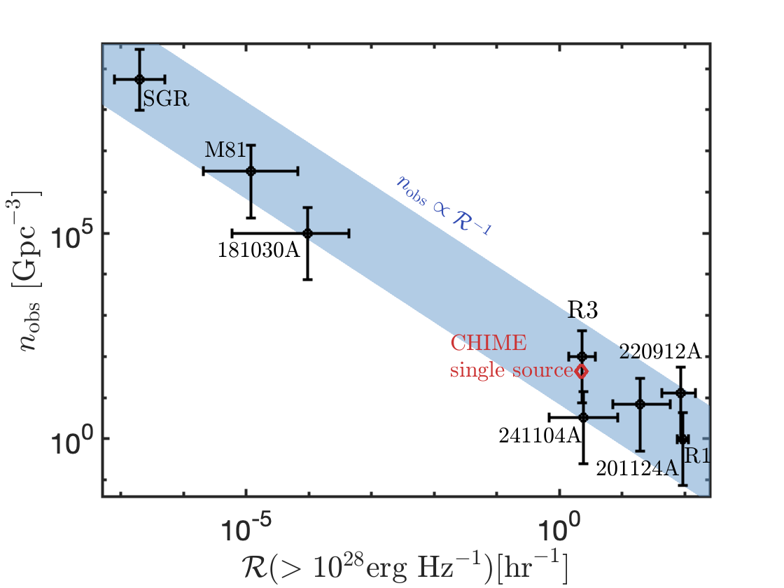
Figure 1: Estimated source number densities of different FRB sub-classes. These are plotted against the rate per source extrapolated to an intermediate common energy of $10^{28}\mbox{erg Hz}^{-1}$ using the measured $\gamma$ or $\gamma\!\approx\!1.7\!\pm\!0.2$ when not available. A diamond indicates the same properties under the assumption (disfavored by our analysis) that a single source type dominates CHIME data. Since the latter is dominated by non-repeaters, this also provides a rough estimate for the number density and rate of CHIME non-repeaters. We find that $n_{\rm obs}\!\mathrel{\raisebox{3.01385pt}{\mbox{$\underset{\vbox{\hbox{$\sim$}}}{\vbox{\hbox{$\propto$}}}$}}}\!\mathcal{R}^{-1}$ over a factor of $\sim\!10^{9}$ in density, suggesting that the large range between common/inactive and rare/active sources might be fit by a single PL distribution with roughly equal contributions at different logarithmic scales.

An alternative, related possibility, is that sources that are more active at a particular energy, may also be able to produce more energetic bursts, i.e. that $\mathcal{R}_{*}$ correlates with $E_{\rm c}$. Such a possibility, and physical motivation for it, is described in appendix §B. As it unavoidably introduces additional apriori free parameters, we apply the principle of Occam’s razor and focus primarily on the case with no such correlation. Future data will determine whether this complication is essential.

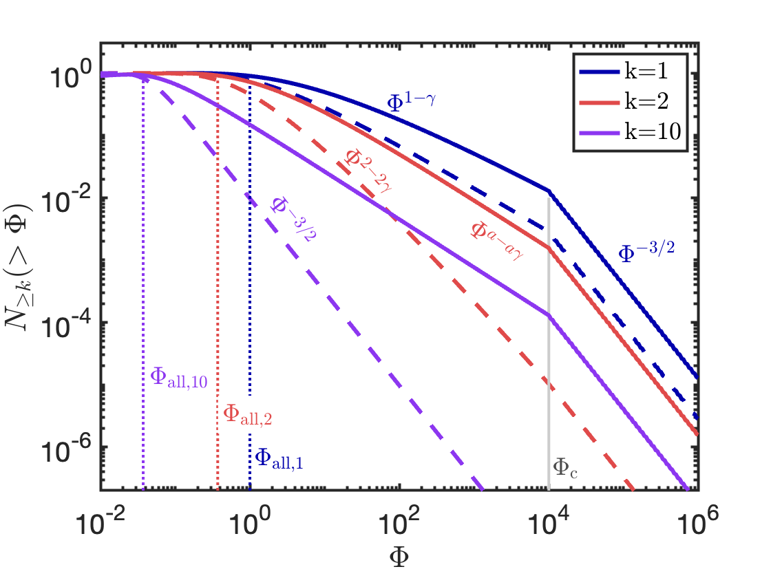
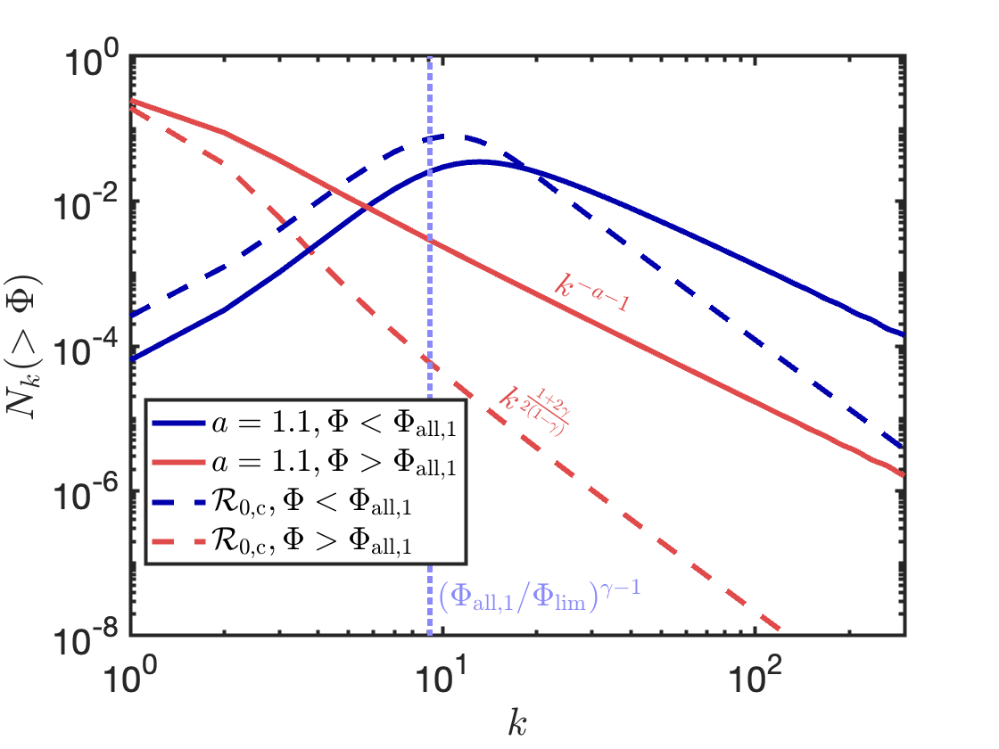
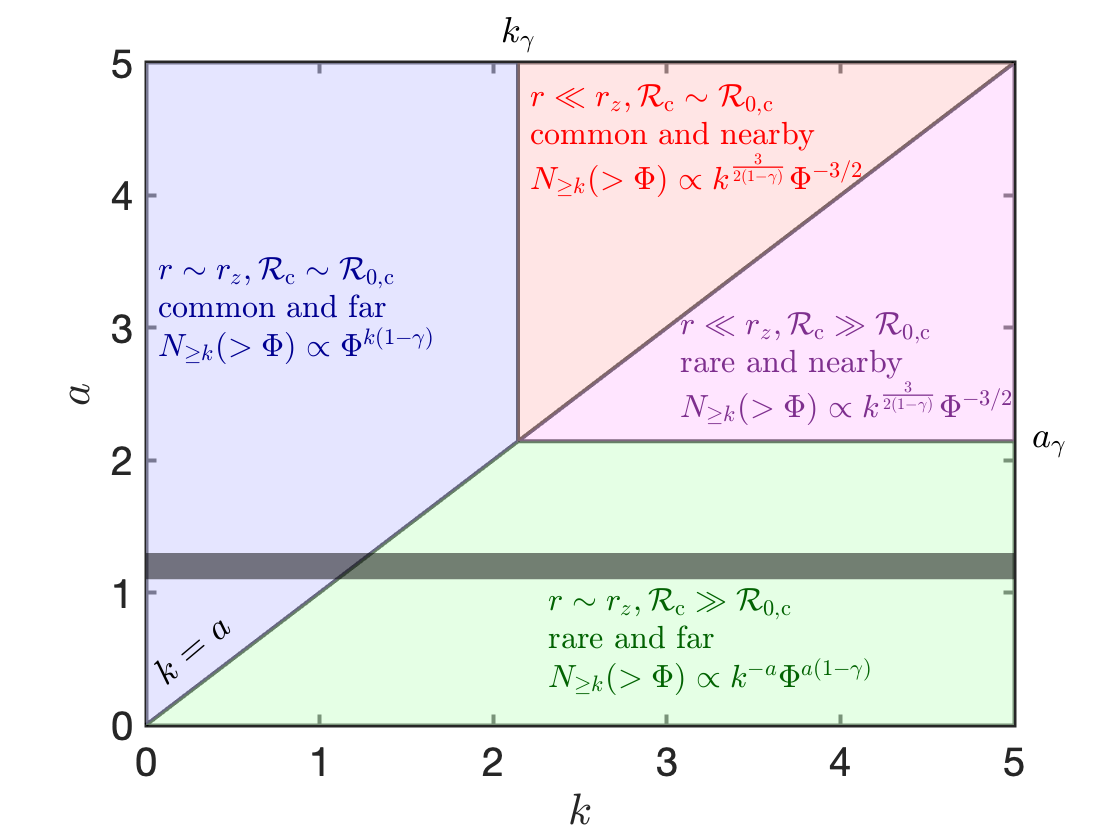
Figure 2: Key results for the distributions of detectable sources. In all panels solid lines depict PL-distributed variable rates, $P(\geq\mathcal{R}_{\rm c})=(\mathcal{R}_{\rm*}/\mathcal{R}_{\rm 0,*})^{-a}$, and dashed lines a constant source rate. Top left: Number of sources above a given fluence with $\geq k$ repeats. For $k>k_{\gamma}$ and $a(\gamma-1)<3/2$, the distribution above $\Phi_{\rm all,k}$ is dominated by gradually rarer and more active sources. Top right: distance distribution of sources observed $\geq k$ times above a fluence $\Phi$. Bottom left: Number of sources observed k times as a function of k. For $\Phi<\Phi_{\rm all,1}$, the distribution peaks at k such that $\Phi_{\rm all,k}=\Phi$ ($k\approx(\Phi_{\rm all,1}/\Phi)^{\gamma-1}$; dotted line), while at larger $k$ the number declines as described in the text. Bottom right: Distances and typical observed activity rate in the parameter space of $a$ (describing the activity rate distribution) and $k$ (number of observed repetitions per source). We also list the dependence of $N_{\geq k}(>\Phi)$ on $k$ and $\Phi$ at the limit of large $k$ and for $\Phi_{\rm all,1}(\mathcal{R}_{\rm 0,c}.)<\Phi<\Phi_{\rm c}$. A shaded region marks the range of $a$ favored by the analysis in §4.

The number of sources observable at $\Phi_{\rm all,k}\!<\!\Phi\!<\!\Phi_{\rm c}$ is given by $\frac{dN_{\geq k}}{d\log\Phi}=\Phi\frac{dN_{\geq k}}{d\mathcal{R}_{\rm*}}\frac{d\mathcal{R}_{\rm*}}{d\Phi}\propto\Phi^{a(1-\gamma)}$ where we have used the fact that $\Phi_{\rm all,k}\propto\mathcal{R}_{\rm*}^{\frac{1}{\gamma-1}}$. This scaling holds as long as it is flatter than the slope given by Eq. 2 (i.e. $a<k$ and $a<k_{\gamma}$). In this regime, common sources dominate at low fluences, and the typical intrinsic rate of an observable source increases with $\Phi$, until, at $\Phi>\Phi_{\rm c}$, the distribution becomes dominated by rare sources with a burst rate of $\mathcal{R}_{\rm*,1}=\mathcal{R}_{\rm 0,*}\lambda_{\rm c}(\mathcal{R}_{\rm 0,*})^{-1}>\mathcal{R}_{\rm 0,*}$. Here, $\mathcal{R}_{\rm*,1}$ is the rate at which bursts with $E_{\rm*}=E_{\rm c}$ repeat at least once during the time $T$, which is equivalent to requiring $\Phi_{\rm all,1}(\mathcal{R}_{\rm c,1})=\Phi_{\rm c}$. It is instructive to consider also the distance distribution of observed sources, for which we estimate

$$\frac{\partial^{2}N_{\geq k}(>\Phi)}{\partial\log r\partial\log\mathcal{R}_{\rm*}}\!=\!4\pi n_{\rm src}r^{3}\!\left(\frac{\mathcal{R}_{\rm*}}{\mathcal{R}_{\rm 0,*}}\right)^{-a}\!P(\geq k|\lambda(\mathcal{R}_{\rm*},r,\Phi))$$

$$\propto r^{3-2k(\gamma-1)}\mathcal{R}_{\rm*}^{k-a}$$ (21)

where the last transition applies when $\lambda\ll 1$. Consider a constant activity rate. We see that while $\lambda\!\gtrsim\!1$, $P\!\sim\!1$ and so $\frac{\partial N_{\geq k}(>\Phi)}{\partial\log r}\!\propto\!r^{3}$ (all sources within limiting volume are visible). This lasts until $r\!\approx\!r_{z}(\Phi_{\rm all,k}/\Phi)^{1/2}$, beyond which only bursts with $E_{\nu}\!>\!E_{\rm all,k}$ are visible and $\frac{\partial N_{\geq k}(>\Phi)}{\partial\log r}\propto r^{3-2k(\gamma-1)}$ (which can have a positive or negative slope depending on $k/k_{\gamma}$). In particular, for $k\gg k_{\gamma}$, one finds that $r_{\rm typ}\propto k^{1\over 2(1-\gamma)}$ (Eq. 6) and $N_{\geq k}(>\Phi)\!\propto\!r_{\rm typ}^{3}\!\propto\!k^{3\over 2(1-\gamma)}$ (or equivalently $N_{k}(>\Phi)\!\propto\!k^{1+2\gamma\over 2(1-\gamma)}$).

For a variable rate, the results remain qualitatively similar so long as $k\!\lesssim\!a$, such that the most common sources, with $\mathcal{R}_{\rm*}\!\approx\!\mathcal{R}_{\rm 0,*}$ dominate. Since $E_{\rm all,k}$ increases with $R_{\rm*}$, for $k\!>\!a$ and $r\!>\!r_{z}\sqrt{\Phi_{\rm all,k}(\mathcal{R}_{\rm 0,*})/\Phi}$, sources with a rate such that $E_{\nu}\!=\!E_{\rm all,k}(\mathcal{R}_{\rm*})$ dominate. This leads to $\mathcal{R}_{\rm*}\!\propto\!r^{2(\gamma-1)}$ and using Eq. 3 to $\frac{\partial N_{\geq k}(>\Phi)}{\partial\log r}\propto r^{3-2a(\gamma-1)}$. The implication is that there is a critical value of $a\!\equiv\!a_{\gamma}\!=\!k_{\gamma}$, such that for $a\!<\!a_{\gamma}\&k$, most observed sources are distant and rare, while for $k\!>\!a\!>\!a_{\gamma}$, sources seen with $k$ times are preferentially nearby and are associated with intrinsically active objects. The results of the fluence and distance distributions with variable source rates, as well as the qualitative behavior in the $a-k$ parameter space, are illustrated in Fig. 2. They can be divided into three cases:

1. $a\!<\!a_{\gamma}\!=\!k_{\gamma}$ - The least active of the observed sources (with $k\!<\!a$), are common (i.e. typical activity rate) and far ($r\!\sim\!r_{z}$). For larger $k\!>\!a$, the typical observed sources are instead dominated by rare (intrinsically highly active) and far sources. In this case $N_{\geq k}(>\!\Phi)\!\propto\!(\Phi/\Phi_{\rm all,k})^{a(1-\gamma)}\!\propto\!k^{-a}$ (or equivalently $N_{k}(>\!\Phi)\!\propto\!k^{-a-1}$). The number of sources with a given repetition number falls off slower than for the constant rate case.

2. $a\!>\!a_{\gamma}\!=\!k_{\gamma}$ - Sources observed with $k\!<\!k_{\gamma}$ are common (i.e. typical activity rate) and far ($r\!\sim\!r_{z}$). Sources seen $k_{\gamma}\!<\!k\!<\!a$ are common and nearby ($r\!\ll\!r_{z}$). Finally, the sources seen to repeat most often, with $k\!>\!a\!>\!k_{\gamma}$, are both rare and nearby.

3. Single activity rate - $a\!\to\!\infty$. It is equivalent to the previous case, but where only the first two $k$ regimes are applicable.

4 Inferences from observations

With approximately one MW-like galaxy per $100\mbox{Mpc}^{3}$, we can estimate the number density of FRB-producing magnetars in the local Universe as $10^{7}-3\times 10^{8}\mbox{Gpc}^{-3}$ (the range corresponding to either 1 or all magnetars in the Galaxy being potential FRB sources; for quantitative estimates below, we take the logarithmic mean). We use this to calculate the total number of FRB producing magnetars in the Universe, $N_{\rm src}\!\sim\!7\!\times\!10^{11}$, assuming that the magnetar density approximately tracks the star formation rate. At the same time, the number of sources seen by CHIME once or more during the period of data collection for the first CHIME catalog is only, $N_{\geq 1,\rm CH}=492$ and the number of sources observed at least twice (repeaters), $N_{\geq 2,\rm CH}=16$ (CHIME/FRB Collaboration et al., 2021). Correcting for the fraction of the sky viewable by CHIME, $f_{\rm FoV}\approx 0.5$, we see that

$$\frac{N_{\rm\geq 1,CH}}{N_{\rm\geq 0,CH}}\approx 1.3\times 10^{-9\pm 0.74}\quad;\quad\frac{N_{\rm\geq 2,CH}}{N_{\rm\geq 1,CH}}\approx 0.03$$ (22)

FRB 20200428 had an energy of $\sim 10^{26}\mbox{ erg Hz}^{-1}$ (Bochenek et al., 2020). The rate of bursts of comparable energy from a given active magnetar in the Galaxy are constrained by over two years of observations by STARE2 and by $\sim 1.5$ years of observations by its successor GReX (Connor et al., 2021; Shila et al., 2025). These observations reduce the rate estimate based on STARE2 (e.g. Margalit et al. 2020; Lu et al. 2022) by a factor of several, resulting in $\mathcal{R}_{0}(\!>10^{26}\mbox{erg Hz}^{-1})\!\approx\!5\!\times\!10^{-6}\mbox{ hr}^{-1}$. From this we see that $\lambda_{0,*}\!\approx\!10^{-4}(E_{*}/10^{26}\mbox{erg Hz}^{-1})^{1-\gamma}$. Observationally, we only have a lower limit on the maximum FRB energy from SGRs $E_{*}\!>\!10^{26}\mbox{ erg Hz}^{-1}$. If $E_{*}\!\gtrsim\!E_{\rm lim}$ then, $\lambda_{\rm lim}\!=\!\lambda_{\rm 0,lim}\!=\!\lambda_{0,*}(E_{\rm lim}/E_{*})^{1-\gamma}\!\approx\!4.5\!\times\!10^{-9}$, which is of the same order as $N_{\geq 1}/N_{\geq 0}$. Is it possible to consistently explain the inferred values of $N_{\geq 1}/N_{\geq 0}$, $N_{\geq 2}/N_{\geq 1}$ and $\lambda_{\rm 0,lim}$?

Consider first the case of a single source type. In this case, since $N_{\geq 2}/N_{\geq 1}\ll 1$, then $\lambda_{\rm lim}\ll 1$, which using Eq. 14 leads to

$$\frac{N_{\geq 1}}{N_{\geq 0}^{\rm sng}}\approx\lambda_{\rm lim}\approx\frac{4N_{\geq 2}}{N_{\geq 1}}\approx 0.05$$ (23)

which is too large by at least seven orders of magnitude (see Eq. 22) .

The difficulty of explaining both the observed ratio of repeaters to non-repeaters and the wide range of activity levels using a single type of source was first highlighted by Margalit et al. (2020). That study proposed a bimodal population, consisting of rare but highly active sources and common but largely inactive ones, to account for the data. However, as shown in Fig. 1, this bimodal model struggles to explain intermediate cases, such as the FRB associated with the M81 galaxy. Instead, the data suggest a continuous PL distribution, spanning from the most common, least active sources to the rarest, most active ones. It is this continuous framework that we explore below.

We take a distribution of source rates $P(\geq\mathcal{R}_{\rm*})=(\mathcal{R}_{\rm*}/\mathcal{R}_{\rm 0,*})^{-a}$ with $a>0$, so that observed CHIME bursts might be dominated by a rare but prolific population of FRB repeaters (see §3). The ratios $N_{\geq 1}/N_{\geq 0},N_{\geq 2}/N_{\geq 1}$ depend on the value of $a$

$${\small\frac{N_{\geq 1}}{N_{\geq 0}}\!\approx\!\left\{\begin{array}[]{ll}\!\lambda_{\rm lim}^{a}&0\!<\!a\!<\!1\\ \!\lambda_{\rm lim}&a>1\ .\end{array}\right.;\frac{N_{\geq 2}}{N_{\geq 1}}\!\approx\!\left\{\begin{array}[]{ll}\!2^{-a}&0\!<\!a\!<\!1\\ \!\frac{\lambda_{\rm lim}^{a-1}}{2^{a}}&1\!<\!a\!<\!2\\ \!\frac{\lambda_{\rm lim}}{4}&a>2\ .\end{array}\right.}$$ (29)

and $\lambda_{\rm lim}\approx\lambda_{\rm 0,lim}$ as before. For $a<1$, the fraction of repeaters is too large $N_{\geq 2}/N_{\geq 1}\geq 2^{-a}>1/2$, while for $a>2$, the estimate in Eq. 23 is approximately applicable, and once more the total number of sources is much too low. However, for intermediate values of $1<a<2$, and specifically, for $a-1\ll 1$, one finds that $N_{\geq 1}/N_{\geq 0}\approx\lambda_{\rm 0,lim}\ll N_{\geq 2,\rm CH}/N_{\geq 1,\rm CH}$. Indeed taking $a\approx 1.13$ simultaneously reproduces all three observables. As mentioned above, the simple analytic estimate needs to be adjusted to account for a few effects: (i) A more realistic, not broken PL approximation of $N_{\geq k}(>\Phi)$, (ii) cosmological distance, time dilation and frequency redshift corrections, (iii) The average spectrum of FRB sources, suggesting that bursts are less common at high frequencies and (iv) the non-uniform observation time spent by a large sky survey per point in the observed sky. These factors are all accounted for by direct numerical integration in §A. The results are shown in Fig. 3. As seen in the figure, the analytic result quoted above is well reproduced by this more precise calculation. The results of the latter, indicate that $1.1\lesssim a\lesssim 1.3$ can simultaneously match the observed $N_{\geq 1}/N_{\geq 0}$, $N_{\geq 2}/N_{\geq 1}$ and $\lambda_{\rm 0,lim}$.

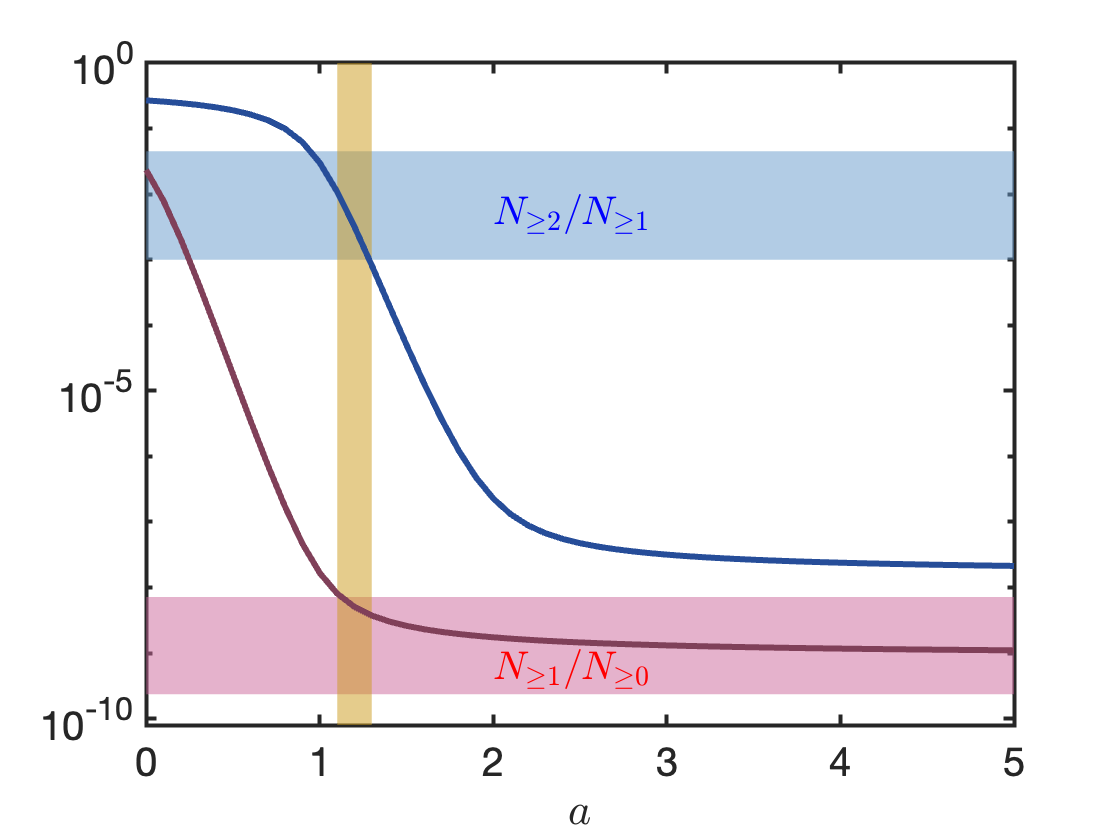
Figure 3: Ratio of repeaters to non-repeaters (blue) and of non-repeaters to all sources (red) as a function of the PL index $a$, considering an observation strategy consistent with CHIME’s 1st catalog. We assume $\mathcal{R}_{\rm 0}(>10^{26}\mbox{erg Hz}^{-1})=5\times 10^{-6}\mbox{hr}^{-1},E_{\rm c}=3\times 10^{33}\mbox{erg Hz}^{-1},\gamma=1.7$ as inferred from observations. Shaded regions depict the inferred ranges of these properties from observations. Solid lines are the results of numerical integration (Eq. A2). The model matches observations well within the shaded yellow range.

An alternative possible resolution is to assume a connection between source rate and maximum burst energy, the results corresponding to this situation are described in §B.

5 Implications for magnetar sources

Eq. 1 that has been applied here to the rate of bursts per source, has also been shown to hold across the Galactic magnetar population, and across temporally removed burst episodes in individual magnetars (see e.g. Cheng et al. 1996; Göǧüş et al. 1999; Gavriil et al. 2004). Moreover, these studies have found the PL index to be $\gamma\approx 1.7$, consistent with the values inferred for FRBs.

For $\gamma<2$ the emitted power per source (averaged over sufficiently long timescales) is dominated by bursts with energies comparable to the maximal energy, $E_{\rm c}$. The (isotropic equivalent) radio energy released per source during an activity time $t$ is given by $E_{\rm rel}\approx 6\times 10^{36}(\mathcal{R}_{*}/\mathcal{R}_{0,*})(t/30\mbox{ yr})(E_{\rm c}/E_{\rm lim})^{2-\gamma}\mbox{ erg}$. Since we infer $|a-1|\ll 1$, there is large probability of detecting sources with $\mathcal{R}_{*}\gg\mathcal{R}_{0,*}$ and indeed such sources should dominate the population of CHIME repeaters (see Fig. 2). As shown in Fig. 1, for R1-type sources, $\mathcal{R}_{*}/\mathcal{R}_{0,*}\approx 3\times 10^{8}$. This leads to $E_{\rm rel,R1}\approx 1.8\times 10^{45}$ for the same beaming factor, radio efficiency and activity time, as consistent with the independent estimate $E_{\rm rel,R1}\approx 8.4\times 10^{44}\mbox{ erg}$ done in Beniamini & Kumar (2025). For an extremely active source such as R1, Beniamini & Kumar (2025) have shown that the magnetic energy reservoir becomes constraining and special conditions have to be met to satisfy it (e.g. regarding the alignment of magnetic, rotation and viewing angle axes as well as the age of the source and its internal magnetic field strength).

6 Conclusions

We have investigated the hypothesis that all FRBs originate from repeating sources. While the intrinsic repetition rates of individual sources at a fixed energy, $\mathcal{R}_{*}$, span a wide range, we find that the inferred number density of similarly active sources, $n_{\rm obs}$ varies correspondingly. Remarkably, these two quantities follow a simple inverse relationship, well described by a Zipf-like law: $n_{\rm obs}\mathrel{\raisebox{3.01385pt}{\mbox{$\underset{\vbox{\hbox{$\sim$}}}{\vbox{\hbox{$\propto$}}}$}}}\mathcal{R}_{*}^{-1}$, extending across approximately 8–9 orders of magnitude. Zipf’s law—where frequency scales inversely with rank—has been observed in numerous natural systems. In astrophysics, similar patterns have been noted in the distributions of solar flares (Lu & Hamilton, 1991) lunar crater sizes (Neukum & Ivanov, 1994), and the size distributions of both cosmic voids (Gaite, 2005) and superclusters (De Marzo et al., 2021).

The applicability of Zipf’s law to FRBs is derived directly from observational data. It implies that the effective distribution of intrinsic repetition rates (above a fixed energy) follows a PL: $P(>\mathcal{R}_{*})\propto\mathcal{R}_{*}^{-a}$ with $a$ close to unity. We explored the implications of such a distribution for the observable properties of FRBs detected in wide-field surveys such as ASKAP, DSA, and CHIME. Specifically, we computed the expected distributions of fluence, distance, and observed repetition number as functions of $a$ and $\gamma$ (where $\gamma$ is the PL index describing the burst energy distribution from individual sources). Our analysis shows that the behavior of the FRB population can be qualitatively divided into four distinct regimes in the $a-k$ parameter space (with $k$ denoting the number of observed bursts from a source), depending on the relationship between $a,k$, and the critical value $a_{\gamma}=k_{\gamma}=3/(2(\gamma-1))$. For typical observed values - $\gamma\approx 1.7$ and $a\approx 1$ - repeaters are dominated by a small number of highly active sources, while non-repeaters include comparable contributions from both rare, active sources and more common, intrinsically inactive ones. All observed FRBs tend to originate from distant sources, although repeaters are, on average, slightly closer than non-repeaters (consistent with trends in dispersion measures; see Fig. 5). A much sharper distinction exists between sources that are observed at least once and those that are never detected. The latter are predicted to be far more numerous and significantly less active. For example, the corrected repetition rate of SGR 1935+2154 (accounting for the observed energy of its bursts) yields an expected detection rate (above CHIME threshold) of only $\sim few\times 10^{-9}$ bursts per such source at cosmological distances—comparable to the inferred ratio of CHIME-detected sources to the estimated number of inactive, SGR-like sources in the Universe. This apparent coincidence emerges naturally if the source repetition rate distribution follows a power law with index $a\approx 1.1-1.3$. Notably, the same distribution also reproduces the observed ratio between CHIME repeaters and apparent non-repeaters. Since $a-1\ll 1$, the relative fraction of repeaters increases only very slowly with increased observation time or improved sensitivity (as $N_{\geq 2}/N_{\geq 1}\propto(\Phi_{\rm lim}^{1-\gamma}T)^{a-1}$ see §A and Fig. 5). This weak dependence could be misinterpreted as evidence that repeaters and non-repeaters represent fundamentally different source populations, even if all FRBs originate from the same underlying class.

A key strength of our analysis is its independence from any specific progenitor or emission model. Nonetheless, the consistency of the least active FRB sources with known Galactic SGRs, combined with the success of a single PL of the activity-rate distribution in explaining the full observed population, naturally points to magnetars as the dominant—or possibly sole—origin of FRBs. What then accounts for the wide variation in inferred source densities and activity levels among different magnetars? Beniamini & Kumar (2023, 2025) suggest that the inclination between spin and magnetic axes ($\alpha$) can play a major role in understanding various apparent differences between repeaters and non-repeaters (including rate, source densities and energetics as relevant for the present analysis, but also resolving the lack of rotational periodicity in arrival time data of active repeaters, explaining the lack of polarization angle in active repeaters compared to polarization angle swing seen in some non-repeaters, providing a geometrical explanation for the CHIME spectro-temporal dichotomy and explaining the periodic modulation within the duration of the long non-repeating FRB 20191221A). This raises the question - what fraction of the spread in inferred source densities can be accounted for by magnetic inclination? The fraction of the sky that is illuminated by a given misaligned NS’s polar cap is $\propto\sin\alpha\approx\alpha$. The intrinsic probability of the inclination being $\leq\alpha$, $P_{\rm int}(<\alpha)$, depends on the initial distribution and on potential alignment that may take place as the magnetar evolves, both of which are uncertain. Therefore, all else being equal, the probability to observe a NS with inclination smaller than $P_{\rm ob}(<\alpha)$ is $\sim P_{\rm int}(<\alpha)\alpha$. An illustrative example is the case of a purely isotropic distribution. In this case we have $P_{\rm int}\propto\alpha^{2}$ and $P_{\rm ob}(<\alpha)\propto\alpha^{3}$. This holds for $\rho\lesssim\alpha\lesssim\pi/2$ where $\rho$ is the half opening angle of the polar cap in the observer frame. Considering likely values of the spin period, one might expect $10^{-2.5}\lesssim\rho\lesssim 10^{-1.5}$. Therefore, it is plausible that $\alpha^{3}$ varies by up to $\sim 7.5$ orders of magnitude and that inclination plays a significant and perhaps even the major rule in explaining the inferred source density variations. The rotation of the emission beam also affects the observed rate, which will increase with decreasing $\alpha$ according to $\mathcal{R}_{\rm ob}\propto\alpha^{-1}\mathcal{R}_{\rm int}(\alpha)$, where $\mathcal{R}_{\rm int}(\alpha)$ is the intrinsic dependence of the rate on $\alpha$. Agreement with the inferred $a\approx 1.1-1.3$ requires (for an isotropic inclination distribution) that $\mathcal{R}_{\rm int}(\alpha)\mathrel{\raisebox{3.01385pt}{\mbox{$\underset{\vbox{\hbox{$\sim$}}}{\vbox{\hbox{$\propto$}}}$}}}\alpha^{-1.8}-\alpha^{-1.3}$. Whether or not this can be reconciled depends on uncertain bursting properties and is an interesting topic for future investigations. Variation in other properties such as magnetic field strength or age—as well as temporal variations in burst rate, energy distribution slope $\gamma$, or maximum burst energy—can also partially contribute to the intrinsic rate - source density Zipf law. Finally, an alternative possibility relates to the presence of a rare sub-population of ultra-long-period magnetars that might be especially prolific FRB emitters (see e.g. Beniamini et al. 2020, 2023). Note that in this case, the polar cap angle can be much smaller than mentioned above, making it easier to explain a large range in rates and source densities, even without a strong dependence of $P_{\rm int}(<\alpha),\mathcal{R}_{\rm int}(\alpha)$ on $\alpha$.

ACKNOWLEDGEMENTS

We thank Zorawar Wadiasingh, Om Gupta and Rob Fender for helpful comments on the manuscript. The work was funded in part by an NSF grant AST-2009619 (PK), a NASA grant 80NSSC24K0770 (PK and PB), a grant (no. 2020747) from the United States-Israel Binational Science Foundation (BSF), Jerusalem, Israel (PB) and by a grant (no. 1649/23) from the Israel Science Foundation (PB).

Appendix A Numerical verification

To verify the validity of our simplifying assumptions presented in the main text, we have carried also a numerical calculation in which we account for appropriate redshift corrections, as well for a realistic distribution of observation time per location on the sky.

In particular, we assume the distribution of FRB sources, $n_{\rm src}(z)$ is proportional to the cosmic SFR (Gupta et al., 2025),

$$n_{\rm src}(z)=A_{\rm src}^{\rm sfr}\dot{m}_{\ast}(z)=A_{\rm src}^{\rm sfr}\begin{cases}0.015\dfrac{(1+z)^{2.73}}{1+[(1+z)/3]^{6.24}}&\text{if }0<z<4,\\ 10^{-0.257z-0.275}&\text{if }4\leq z\leq 14.\end{cases}M_{\odot}\mbox{ yr}^{-1}\mbox{ Mpc}^{-3}.$$ (A1)

where $A_{\rm src}^{\rm sfr}$ is the conversion fraction from star formation rate to population density of FRB sources. If the latter are magnetars, then approximately, $A_{\rm src}^{\rm sfr}\approx 20\mbox{yr}M_{\odot}^{-1}$ (corresponding to roughly 30 magnetars in the Milky Way and a number density of Milky-Way like galaxies of $\sim 0.01\mbox{ Mpc}^{-3}$). Some recent studies (Qiang et al., 2022; Zhang & Zhang, 2022; Lin & Zou, 2024; Gupta et al., 2025; Horowicz & Margalit, 2025; Acharya & Beniamini, 2025) have suggested that FRBs arising from a mix of SFR and stellar mass following populations, fit better with the observed redshift and host galaxy distributions. Such a possibility is straightforward to include in this analysis. Since its effect on the results of this study are minor and in order to avoid introducing additional weakly constrained parameters, we ignore this complication in the estimates below. We assume also that the average spectrum of FRBs can be characterized using $E_{\nu}\propto\nu^{\alpha}$. Previous studies (Macquart et al., 2019; Shin et al., 2023) have found $\alpha\approx-1.5$. The measured fluence of an FRB is then given by $\Phi=E_{\nu_{0}}(1+z)^{\alpha}/(4\pi r^{2})$ where $\nu_{0}$ is the frequency at which the fluence is measured, $r$ is the proper distance and the factor $(1+z)^{\alpha}$ is a $k$-correction, i.e. converting from the measured $\nu_{0}$ to the corresponding frequency in the comoving frame $\nu=\nu_{0}(1+z)$.

We consider a non-uniform distribution of observation time per location on the sky viewed by the survey, $d\mbox{P}/dT$. For our numerical calculations we use the distribution reported in the first CHIME catalog (CHIME/FRB Collaboration et al., 2021). This corresponds to a median observation time of $\sim 20$ hrs, but with some locations observed for much longer times.

Taking all these ingredients together, we may calculate the number of bursts detected $k$ times during a survey

$$N_{\geq k}=\frac{\Omega_{\rm srv}}{4\pi}\int_{0}^{\infty}dT\int_{\mathcal{R}_{\rm 0,*}}^{\infty}d\mathcal{R}_{\rm*}\int_{0}^{\infty}dV(z)\frac{d\mbox{P}}{dT}\frac{d\mbox{P}}{d\mathcal{R}_{\rm*}}n_{\rm src}(z)\mbox{Pois}\left(k\bigg{|}\frac{T}{1+z}\mathcal{R}_{\rm*}\left[\frac{E_{\rm lim}(z)}{E_{\rm*}}\right]^{1-\gamma}\right)\Theta(E_{\rm c}-E_{\rm lim}(z))$$ (A2)

where $\Omega_{\rm srv}/4\pi$ is the fraction of the sky viewed by the survey (approximately 0.5 for CHIME), $\Phi_{\rm lim}$ is the limiting (spectral) fluence of the survey and $E_{\rm lim}(z)=4\pi r^{2}\Phi_{\rm lim}(1+z)^{-\alpha}$. $d\mbox{P}/d\mathcal{R}_{\rm*}\propto\mathcal{R}_{\rm*}^{-a-1}$ is the probability of a source having a given intrinsic rate (at $E_{\rm*}$). Pois$(k|\lambda)$ is the Poisson probability distribution of observing $k$ events considering an expected value of $\lambda$. The value $\lambda=\frac{T}{1+z}\mathcal{R}_{\rm*}\left[\frac{E_{\rm lim}(z)}{E_{\rm*}}\right]^{1-\gamma}$ accounts for the rate of the source above the minimum energy detectable by the survey and considering the (comoving) time that it has been observed by the survey.

The results of numerical integration for $N_{\geq 2}/N_{\geq 1},N_{\geq 1}/N_{\geq 0}$ as a function of $a$ were shown in Fig. 3 where it was shown that $1.1\lesssim a\lesssim 1.3$ can simultaneously match the observed $N_{\geq 1}/N_{\geq 0}$, $N_{\geq 2}/N_{\geq 1}$ and $\lambda_{\rm 0,lim}$. Fig. 4 shows how the ratio of repeaters to total detected sources, $N_{\geq 2}/N_{\geq 1}$, evolves for a fixed value of $a=1.1$ , as a function of decreasing the fluence threshold or increasing the average observation time per sky location. For a small value of $a-1$, the analytic expression $N_{\geq 2}/N_{\geq 1}\propto(\Phi_{\rm lim}^{1-\gamma}T)^{a-1}$ (Eq. 29) predicts that the repeater fraction depends only weakly on both limiting fluence and observing time. This weak dependence is confirmed by our numerical results: increasing the observation time by a factor of 10 leads to only a modest increase - by a factor of $\sim 1.8$ - in the fraction of repeaters. Reducing the fluence threshold by a similar factor yields an even smaller effect. The figure also illustrates how the repeater fraction varies across the sky, based on the relation between exposure time and declination in the first CHIME catalog. Since CHIME observes higher declinations for longer, the fraction of repeaters is slightly elevated in those regions. However, this variation is relatively small, again reflecting the weak dependence of the repeater fraction on exposure (as a rough approximation, CHIME’s exposure distribution roughly satisfies $T\propto(\pi/2-\delta)^{-1}$, CHIME/FRB Collaboration et al. 2021, leading to $N_{\geq 2}/N_{\geq 1}\propto(\pi/2-\delta)^{1-a}$). We also show, in Fig. 5. the distribution of distances, external dispersion measures and intrinsic rates for both observed repeaters and non-repeaters. As shown in Fig. 2, for $a=1.1$, both repeaters and non-repeaters are predominantly detected at cosmological distances. Interestingly, repeaters are, on average, a few tens of percent closer than non-repeaters. This leads to typical intergalactic dispersion measures of $\mbox{DM}_{\rm ext,rep}\sim 400\mbox{pc cm}^{-3}$ for repeaters, compared to $\mbox{DM}_{\rm ext,NR}\sim 670\mbox{pc cm}^{-3}$ for non-repeaters—both consistent with observed values (Chime/Frb Collaboration et al., 2023). This agreement is particularly striking given that our modeling was developed independently of dispersion measure data, using a simple framework and approximate detectability criteria. While the two populations show some overlap in distance, they differ much more clearly in their intrinsic repetition rates: repeaters are dominated by the rarest and most active sources, whereas the non-repeater population includes a roughly equal mix of common, inactive sources and rare, highly active ones.

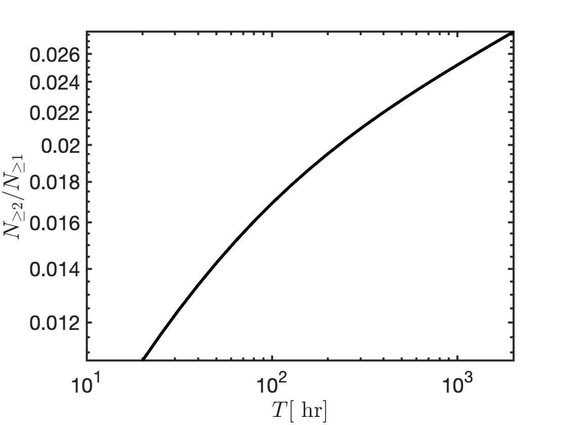
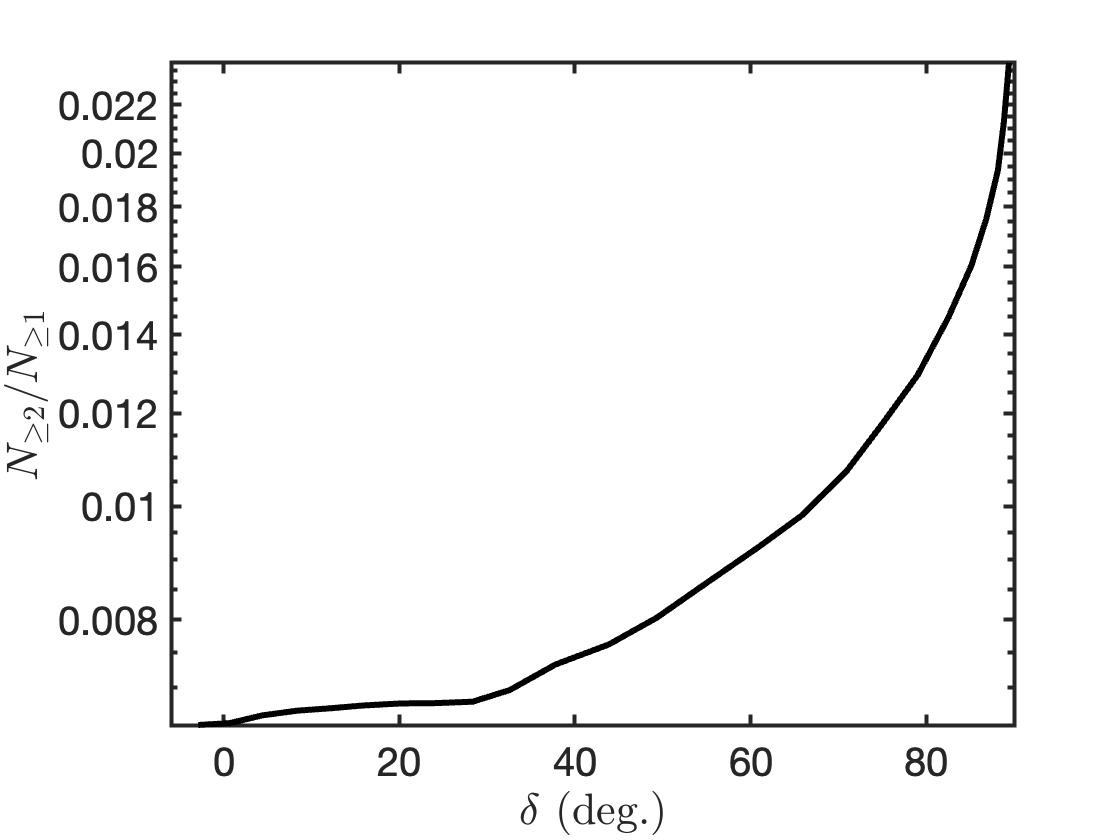
Figure 4: Fraction of observable repeaters as a function of the limiting fluence (left) and as a function of mean observation time per sky location (center) using a fluence threshold of 5Jy ms (marked by an asterisk on the left panel). In both cases we adopt $a=1.1$, consistent with observational constraints (see Fig. 3). The repeater fraction is very weakly dependent on either $T$ or $\Phi$. The right panel shows how the repeater fraction changes with declination assuming the distribution of exposure vs. declination from the first CHIME catalog.

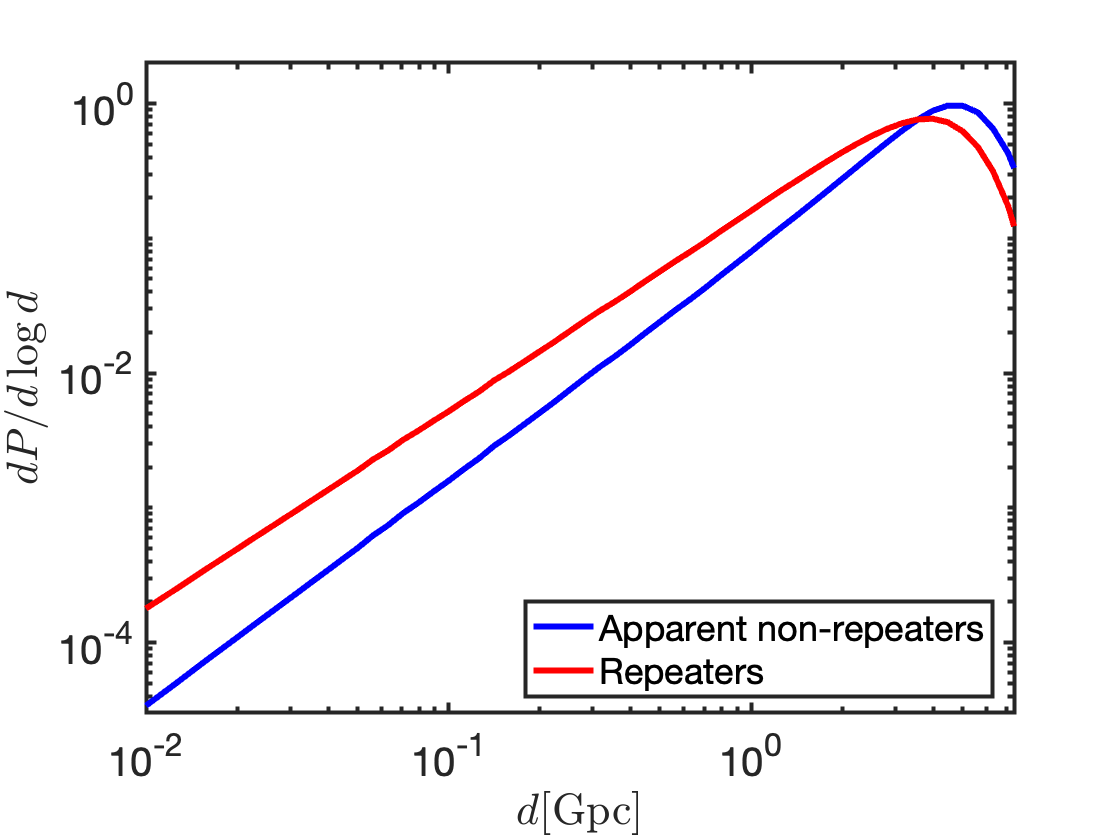
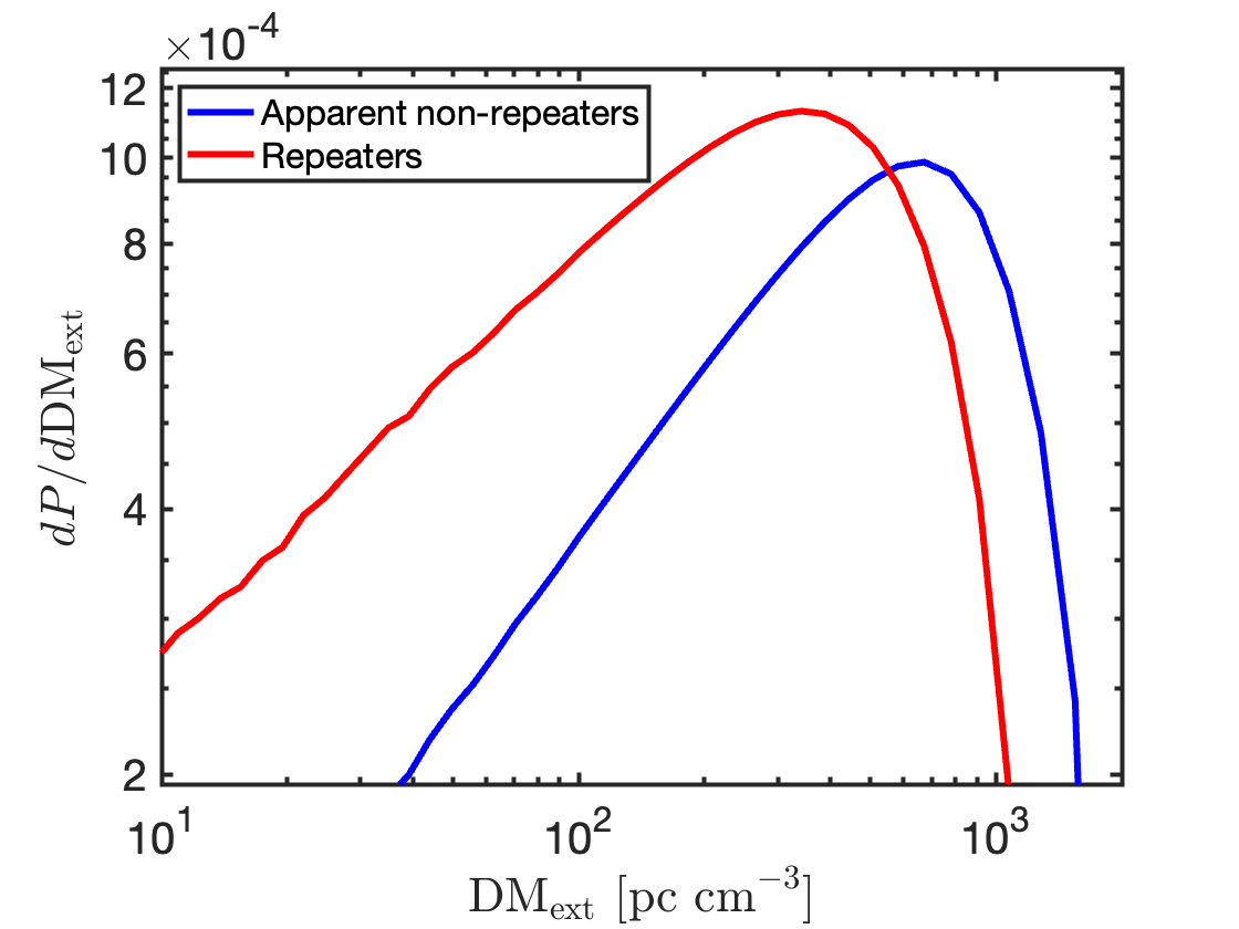
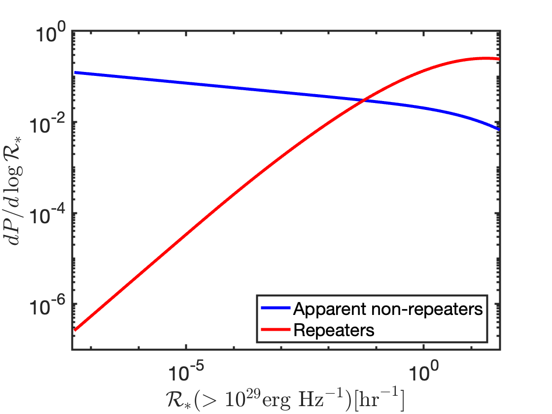
Figure 5: Distance (left), external DM (due to propagation in the intergalactic medium) and activity rate (right) distributions of repeaters and non-repeaters. Results are shown for $a=1.1$ and other parameters as in described in appendix A and Fig. 4. For DM_ext we use DM${}_{\rm ext}=855z\mbox{pc cm}^{-3}$, which is applicable for the $z\lesssim 3$ population that dominates the CHIME detected population.

Appendix B Correlation between rate and maximal energy

The activity rate of sources (at some fixed energy) may be correlated with the maximum burst energy. This is a natural expectation of at least some relevant physical scenarios. For example, for magnetar sources, both quantities are likely positively correlated with the magnetar’s internal field strength (Beniamini et al., 2025). We assume a PL relation, $E_{\rm c}=E_{*}(\mathcal{R}_{*}/\mathcal{R}_{0,*})^{b}$, where $\mathcal{R}_{0,*}$ is the rate of bursts (per source) at $E_{*}$ for sources for which $E_{*}$ is the maximum burst energy and $\mathcal{R}_{*}$ is the rate of bursts per source at the same energy for sources for which $E_{\rm c}$ is the maximum burst energy. It is convenient to choose $E_{*}$ as the maximum energy of the most common (and least active sources). $b=0$ corresponds to the case discussed in §3. Instead, for $b>0$, if $E_{\rm lim}>E_{*}$, then detection of bursts from sources for which $E_{\rm lim}>E_{\rm c}$ is suppressed. This leads to a minimum rate at $E_{*}$, $\mathcal{R}_{*}=\mathcal{R}_{0,*}(E_{\rm lim}/E_{*})^{1/b}$. Using $P(>\mathcal{R}_{*})\propto\mathcal{R}_{*}^{-a}$ we see that these sources, with $E_{\rm c}\approx E_{\rm lim}$ represent a small fraction, of order $(E_{\rm lim}/E_{*})^{-a/b}$ relative to the most common, and least active sources. The mean number of detectable bursts produced by such sources is $\lambda_{\rm lim}=\lambda_{0,*}(E_{\rm lim}/E_{*})^{1-\gamma+1/b}$. There is therefore a critical value of $b=b_{c}\equiv 1/(\gamma-1)$, such that for $b\ll b_{c}$, $\lambda_{\rm lim}\gg\lambda_{0,*}$. In particular, if $\lambda_{\rm lim}>1$, this implies that most observed sources will be observed multiple times. As $b$ grows, $\lambda_{\rm lim}$ drops and so does the relative frequency of sources detected multiple times. Moreover, since $\Phi_{\rm all,k}\propto\mathcal{R}_{*}^{1/(\gamma-1)}$ while $\Phi_{\rm c}\propto\mathcal{R}_{*}^{b}$ we see that for $b<b_{c}$ $\Phi_{\rm c}$ grows more slowly with an increasing rate than $\Phi_{\rm all,k}$. This means that there is a critical rate (or $\lambda$) for which the two become equal $\bar{\lambda}=\lambda_{0,*}^{-b(1-\gamma)\over 1-b\gamma+b}k^{1\over 1-b\gamma+b}$ and a corresponding fluence $\bar{\Phi}=\Phi_{*}(k/\lambda_{0,*})^{b\over 1-b\gamma+b}\gg\Phi_{*}$ (note that $\bar{\Phi}$ increases with $k$). Analogously to the discussion in §3, for $\Phi<\bar{\Phi}$ $N_{\geq k}(>\Phi)\propto\Phi^{a(1-\gamma)}k^{-a}$ and for $\Phi>\bar{\Phi}$, $N{\geq k}(>\Phi)\propto(\bar{\Phi}/\Phi_{\rm all,k})^{-a(\gamma-1)}(\Phi/\bar{\Phi})^{-3/2}\propto\Phi^{-3/2}k^{-a+\frac{b[3/2-a(\gamma-1)]}{1-b(\gamma-1)}}$. Instead, for $b>b_{c}$, $\Phi_{\rm c}$ grows faster than $\Phi_{\rm all,k}$ and as a result $N(>\Phi)\propto\Phi^{a(1-\gamma)}k^{-a}$ holds up to arbitrarily large $\Phi$.

As explained above only a fraction $(E_{\rm lim}/E_{*})^{-a/b}$ of all sources are detectable above $\Phi_{\rm lim}$ and they are characterized by $\lambda_{\rm lim}=\lambda_{0,*}(E_{\rm lim}/E_{*})^{1-\gamma+1/b}$. Requiring $N_{\geq 2}/N_{\geq 1}\ll 1$, leads to $\lambda_{\rm lim}\ll 1$ and in turn to

$$\frac{N_{\geq 1}}{N_{\geq 0}}\!\approx\!\left(\frac{E_{\rm lim}}{E_{*}}\right)^{-\frac{a}{b}}\left\{\begin{array}[]{ll}\!\lambda_{\rm lim}^{a}&0\!<\!a\!<\!1\\ \!\lambda_{\rm lim}&a>1\ .\end{array}\right.\approx\lambda_{\rm 0,*}\left\{\begin{array}[]{ll}\!\left(\frac{E_{\rm lim}}{E_{*}}\right)^{1-\gamma}&0\!<\!a\!<\!1\\ \!\left(\frac{E_{\rm lim}}{E_{*}}\right)^{\frac{1-a}{b}+1-\gamma}&a>1\ .\end{array}\right.$$ (B5)

where $E_{*}$ is the maximum energy of bursts from SGR-like sources and $\lambda_{0,*}$ is the mean number of bursts produced by such a source at this typical energy and where the relation between $N_{\geq 2}/N_{\geq 1}$ and $\lambda_{\rm lim}$ is still described by Eq. 29.

While fixing the rate of SGRs at $10^{26}\mbox{erg Hz}^{-1}$ as above (and taking $a>1$), there is an approximate degeneracy in $E_{*},b$, for a given value of $a$ (which leaves $N_{\geq 2}/N_{\geq 1}$ and $N_{\geq 1}/N_{\geq 0}$ unchanged). This means that there are effectively only two parameters (which can be chosen as $a$ and $E_{*}(b)$ that are needed to uniquely determine $N_{\geq 2}/N_{\geq 1}$ and $N_{\geq 1}/N_{\geq 0}$. This degeneracy holds as long as $E_{*}<E_{\rm lim}\approx 1.6\times 10^{32}\mbox{erg Hz}^{-1}$. The numerical evaluation of Eq. A2 accounting for the rate - maximal energy correlation, give $a\approx 1.1$ and $E_{*}\approx 10^{32.2-3.47b}\mbox{erg Hz}^{-1}$.

For $b>0$, sources dominating the CHIME sample, satisfy $\lambda_{\rm CH}(E_{\rm c})=\lambda_{0,*}(E_{*}/10^{26}\mbox{erg Hz}^{-1})^{1-\gamma}(E_{\rm c}/E_{\rm*})^{1/b+1-\gamma}\approx 1.3\times 10^{-5}(E_{\rm c}/E_{\rm lim})^{1/b+1-\gamma}$ with $E_{\rm c}\geq E_{\rm lim}$, such that the results depend on $b$ for $E_{\rm c}>E_{\rm lim}$. This is more than three orders of magnitude greater than the rate of bursts per SGR as extrapolated to $E_{\rm lim}$. We see also that the (isotropic equivalent) energy needed to power this activity is $E_{\rm rel}\approx t\mathcal{R}_{\rm CH}(E_{\rm c})E_{\rm c}\approx 1.6\times 10^{40}(t/30\mbox{ yr})(E_{\rm c}/E_{\rm lim})^{1/b+2-\gamma}\mbox{ erg}$, where $t$ is the time over which the source has been active at this level. This energy is many orders of magnitude lower than the magnetic energy reservoir of a magnetar ($E_{\rm mag}=1.6\times 10^{49}(B/10^{16})^{2}\mbox{ erg}$), even after accounting for the fact that typically only a small fraction of the dissipated energy may be channeled towards the radio band. Since we infer that $a-1\ll 1$, a wide range of intrinsic source repetition rates should be probed by CHIME sources. Indeed Beniamini & Kumar (2025) found that for R1, the energy requirements result in $E_{\rm rel}\approx 8.4\times 10^{44}\mbox{ erg}$ for the same beaming factor, radio efficiency and activity time, about $3\times 10^{5}$ times larger than for the typical CHIME source, as calculated above.

References

- Acharya & Beniamini (2025) Acharya, S. K., & Beniamini, P. 2025, arXiv e-prints, arXiv:2503.08441, doi: 10.48550/arXiv.2503.08441
- Beniamini & Kumar (2023) Beniamini, P., & Kumar, P. 2023, MNRAS, 519, 5345, doi: 10.1093/mnras/stad028
- Beniamini & Kumar (2025) —. 2025, ApJ, 982, 45, doi: 10.3847/1538-4357/adb8e6
- Beniamini et al. (2023) Beniamini, P., Wadiasingh, Z., Hare, J., et al. 2023, MNRAS, 520, 1872, doi: 10.1093/mnras/stad208
- Beniamini et al. (2020) Beniamini, P., Wadiasingh, Z., & Metzger, B. D. 2020, MNRAS, 496, 3390, doi: 10.1093/mnras/staa1783
- Beniamini et al. (2025) Beniamini, P., Wadiasingh, Z., Trigg, A., et al. 2025, ApJ, 980, 211, doi: 10.3847/1538-4357/ada947
- Bochenek et al. (2020) Bochenek, C. D., Ravi, V., Belov, K. V., et al. 2020, Nature, 587, 59, doi: 10.1038/s41586-020-2872-x
- Cheng et al. (1996) Cheng, B., Epstein, R. I., Guyer, R. A., & Young, A. C. 1996, Nature, 382, 518, doi: 10.1038/382518a0
- CHIME/FRB Collaboration et al. (2021) CHIME/FRB Collaboration, Amiri, M., Andersen, B. C., et al. 2021, ApJS, 257, 59, doi: 10.3847/1538-4365/ac33ab
- Chime/Frb Collaboration et al. (2023) Chime/Frb Collaboration, Andersen, B. C., Bandura, K., et al. 2023, ApJ, 947, 83, doi: 10.3847/1538-4357/acc6c1
- Connor et al. (2021) Connor, L., Shila, K. A., Kulkarni, S. R., et al. 2021, PASP, 133, 075001, doi: 10.1088/1538-3873/ac0bcc
- Cruces et al. (2021) Cruces, M., Spitler, L. G., Scholz, P., et al. 2021, MNRAS, 500, 448, doi: 10.1093/mnras/staa3223
- De Marzo et al. (2021) De Marzo, G., Sylos Labini, F., & Pietronero, L. 2021, A&A, 651, A114, doi: 10.1051/0004-6361/202141081
- Fonseca et al. (2020) Fonseca, E., Andersen, B. C., Bhardwaj, M., et al. 2020, ApJ, 891, L6, doi: 10.3847/2041-8213/ab7208
- Gaite (2005) Gaite, J. 2005, European Physical Journal B, 47, 93, doi: 10.1140/epjb/e2005-00306-1
- Gavriil et al. (2004) Gavriil, F. P., Kaspi, V. M., & Woods, P. M. 2004, ApJ, 607, 959, doi: 10.1086/383564
- Göǧüş et al. (1999) Göǧüş , E., Woods, P. M., Kouveliotou, C., et al. 1999, ApJ, 526, L93, doi: 10.1086/312380
- Gupta et al. (2025) Gupta, O., Beniamini, P., Kumar, P., & Finkelstein, S. L. 2025, arXiv e-prints, arXiv:2501.09810, doi: 10.48550/arXiv.2501.09810
- Hashimoto et al. (2022) Hashimoto, T., Goto, T., Chen, B. H., et al. 2022, MNRAS, 511, 1961, doi: 10.1093/mnras/stac065
- Horowicz & Margalit (2025) Horowicz, A., & Margalit, B. 2025, arXiv e-prints, arXiv:2504.08038, doi: 10.48550/arXiv.2504.08038
- Jahns et al. (2023) Jahns, J. N., Spitler, L. G., Nimmo, K., et al. 2023, MNRAS, 519, 666, doi: 10.1093/mnras/stac3446
- James et al. (2022) James, C. W., Prochaska, J. X., Macquart, J. P., et al. 2022, MNRAS, 510, L18, doi: 10.1093/mnrasl/slab117
- Kirsten et al. (2024) Kirsten, F., Ould-Boukattine, O. S., Herrmann, W., et al. 2024, Nature Astronomy, 8, 337, doi: 10.1038/s41550-023-02153-z
- Konijn et al. (2024) Konijn, D. C., Hewitt, D. M., Hessels, J. W. T., et al. 2024, MNRAS, 534, 3331, doi: 10.1093/mnras/stae2296
- Kumar et al. (2022) Kumar, P., Shannon, R. M., Lower, M. E., et al. 2022, MNRAS, 512, 3400, doi: 10.1093/mnras/stac683
- Li et al. (2021) Li, D., Wang, P., Zhu, W. W., et al. 2021, Nature, 598, 267, doi: 10.1038/s41586-021-03878-5
- Lin & Zou (2024) Lin, H.-N., & Zou, R. 2024, ApJ, 962, 73, doi: 10.3847/1538-4357/ad1b4f
- Lu & Hamilton (1991) Lu, E. T., & Hamilton, R. J. 1991, ApJ, 380, L89, doi: 10.1086/186180
- Lu et al. (2022) Lu, W., Beniamini, P., & Kumar, P. 2022, MNRAS, 510, 1867, doi: 10.1093/mnras/stab3500
- Lu & Piro (2019) Lu, W., & Piro, A. L. 2019, ApJ, 883, 40, doi: 10.3847/1538-4357/ab3796
- Macquart et al. (2019) Macquart, J. P., Shannon, R. M., Bannister, K. W., et al. 2019, ApJ, 872, L19, doi: 10.3847/2041-8213/ab03d6
- Margalit et al. (2020) Margalit, B., Beniamini, P., Sridhar, N., & Metzger, B. D. 2020, ApJ, 899, L27, doi: 10.3847/2041-8213/abac57
- Metzger et al. (2022) Metzger, B. D., Sridhar, N., Margalit, B., Beniamini, P., & Sironi, L. 2022, ApJ, 925, 135, doi: 10.3847/1538-4357/ac3b4a
- Neukum & Ivanov (1994) Neukum, G., & Ivanov, B. A. 1994, in Hazards Due to Comets and Asteroids, ed. T. Gehrels, M. S. Matthews, & A. M. Schumann, 359
- Nimmo et al. (2023) Nimmo, K., Hessels, J. W. T., Snelders, M. P., et al. 2023, MNRAS, 520, 2281, doi: 10.1093/mnras/stad269
- Oostrum et al. (2020) Oostrum, L. C., Maan, Y., van Leeuwen, J., et al. 2020, A&A, 635, A61, doi: 10.1051/0004-6361/201937422
- Oppermann et al. (2018) Oppermann, N., Yu, H.-R., & Pen, U.-L. 2018, MNRAS, 475, 5109, doi: 10.1093/mnras/sty004
- Ould-Boukattine et al. (2024) Ould-Boukattine, O. S., Chawla, P., Hessels, J. W. T., et al. 2024, arXiv e-prints, arXiv:2410.17024, doi: 10.48550/arXiv.2410.17024
- Pleunis et al. (2021) Pleunis, Z., Good, D. C., Kaspi, V. M., et al. 2021, ApJ, 923, 1, doi: 10.3847/1538-4357/ac33ac
- Qiang et al. (2022) Qiang, D.-C., Li, S.-L., & Wei, H. 2022, J. Cosmology Astropart. Phys, 2022, 040, doi: 10.1088/1475-7516/2022/01/040
- Ryder et al. (2023) Ryder, S. D., Bannister, K. W., Bhandari, S., et al. 2023, Science, 382, 294, doi: 10.1126/science.adf2678
- Scholz et al. (2017) Scholz, P., Bogdanov, S., Hessels, J. W. T., et al. 2017, ApJ, 846, 80, doi: 10.3847/1538-4357/aa8456
- Sharma et al. (2024) Sharma, K., Ravi, V., Connor, L., et al. 2024, Nature, 635, 61, doi: 10.1038/s41586-024-08074-9
- Shila et al. (2025) Shila, K. A., Niedbalski, S., Connor, L., et al. 2025, arXiv e-prints, arXiv:2504.18680. https://arxiv.org/abs/2504.18680
- Shin et al. (2023) Shin, K., Masui, K. W., Bhardwaj, M., et al. 2023, ApJ, 944, 105, doi: 10.3847/1538-4357/acaf06
- Shin et al. (2025) Shin, K., Curtin, A., Fine, M., et al. 2025, arXiv e-prints, arXiv:2505.13297. https://arxiv.org/abs/2505.13297
- Thompson & Duncan (2001) Thompson, C., & Duncan, R. C. 2001, ApJ, 561, 980, doi: 10.1086/323256
- Tian et al. (2025) Tian, J., Pastor-Marazuela, I., Rajwade, K. M., et al. 2025, MNRAS, doi: 10.1093/mnras/staf793
- Wadiasingh et al. (2020) Wadiasingh, Z., Beniamini, P., Timokhin, A., et al. 2020, ApJ, 891, 82, doi: 10.3847/1538-4357/ab6d69
- Wang & Yu (2017) Wang, F. Y., & Yu, H. 2017, J. Cosmology Astropart. Phys, 2017, 023, doi: 10.1088/1475-7516/2017/03/023
- Wang et al. (2018) Wang, W., Luo, R., Yue, H., et al. 2018, ApJ, 852, 140, doi: 10.3847/1538-4357/aaa025
- Zhang et al. (2021) Zhang, G. Q., Wang, P., Wu, Q., et al. 2021, ApJ, 920, L23, doi: 10.3847/2041-8213/ac2a3b
- Zhang & Zhang (2022) Zhang, R. C., & Zhang, B. 2022, ApJ, 924, L14, doi: 10.3847/2041-8213/ac46ad
- Zhang et al. (2022) Zhang, Y.-K., Wang, P., Feng, Y., et al. 2022, Research in Astronomy and Astrophysics, 22, 124002, doi: 10.1088/1674-4527/ac98f7
- Zhang et al. (2023) Zhang, Y.-K., Li, D., Zhang, B., et al. 2023, ApJ, 955, 142, doi: 10.3847/1538-4357/aced0b