Matrix Product State on a Quantum Computer
Abstract
Solving quantum many-body systems is one of the most significant regimes where quantum computing applies. Currently, as a hardware-friendly computational paradigms, variational algorithms are often used for finding the ground energy of quantum many-body systems. However, running large-scale variational algorithms is challenging, because of the noise as well as the obstacle of barren plateaus. In this work, we propose the quantum version of matrix product state (qMPS), and develop variational quantum algorithms to prepare it in canonical forms, allowing to run the variational MPS method, which is equivalent to the Density Matrix Renormalization Group method, on near term quantum devices. Compared with widely used methods such as variational quantum eigensolver, this method can greatly reduce the number of qubits used in local optimization, and thus mitigate the effects of barren plateaus while obtaining better accuracy. Our method holds promise for distributed quantum computing, offering possibilities for fusion of different computing systems.
I Introduction
Solving quantum many-body systems is a fundamental challenge. Classical computers usually have to deal with the exponential growth in size of the system to mimic the quantum effects. As Feynman raised the concept of quantum simulations Feynman (1982), quantum computing begins to show its great power for specific tasks and stimulated the possibility of solving these systems with advantages over the classical computers. Quantum algorithms were proposed for efficient quantum simulations, and are promising for a wide range of applications such as condensed matter physics Anderson (1984); Sachdev (2023), quantum chemistry Cao et al. (2019); McArdle et al. (2020), high-energy physics Zohar et al. (2015); Martinez et al. (2016), materials Monroe et al. (2021); Maskara et al. (2025), drug discovery Wong et al. (2023); Santagati et al. (2024), or combinatory optimization tasks Moll et al. (2018); Harrigan et al. (2021).
As the quantum advantages have been demonstrated on both superconducting and photonic platforms Arute et al. (2019); Zhu et al. (2022); Madsen et al. (2022); Zhong et al. (2021); Deng et al. (2023); Acharya et al. (2025); Gao et al. (2025), quantum computing has developed rapidly and is moving towards the noisy intermediate scale quantum (NISQ) era Preskill (2018). However, taking the practical physical devices into consideration, running large-scale quantum algorithms still meets severe challenges. For example, algorithms such as the variational quantum eigensolver (VQE) Peruzzo et al. (2014); Kandala et al. (2017), are troubled with ‘barren plateaus’ Liu et al. (2022); Wang et al. (2021), and are more time consuming to converge to an accurate result. To mitigate these challenges, various distributed quantum frameworks have been proposed. For example, deepVQE can handle large-scale systems with weak correlations among subsystems. Other methods such as circuit cutting Peng et al. (2020); Tang and Martonosi (2022) or hybrid tree tensor networks Yuan et al. (2021) reduce the sizes of quantum circuits, but requires global optimizations, which limits the efficiency.
Fortunately, the hybrid tensor network provides a general framework for transplanting the classical tensor network method onto quantum devices. Tensor networks are powerful numerical tools for solving fundamental problems in quantum many-body systems. Recently, tensor network methods are applied in quantum information, and become one of the most efficient method for simulating quantum circuits Markov et al. (2018); Villalonga et al. (2019, 2020); Guo et al. (2019); Liu et al. (2021); Pan et al. (2022). As one of the most widely used tensor network structures, Matrix Product State (MPS) supports important applications of finding the ground energy of a strongly correlated 1-D many-body system Östlund and Rommer (1995); Hastings (2007); Liu et al. (2020).
In this work, we propose the idea of quantum Matrix Product State (qMPS), and develop the variational quantum MPS (vqMPS) method for quantum simulation, which can be viewed as the quantum version of the Density Matrix Renormalization Group (DMRG) method White (1992); Schollwöck (2011) for near-term quantum devices. This method makes it possible to run large-scale quantum simulations with local optimizations on small-scale subsystems, and can reach comparable or even better accuracy over VQE using much fewer qubits. This can greatly enhance the efficiency for both physical demonstration and numerical simulation. Also, the local optimizations can be distributed on different systems, providing a framework for the fusion of different physical platforms, or further quantum-classical hybrid computing.
II The quantum MPS
A classical MPS contains a group of rank-3 tensors at the -th site. The left and right dimensions ( and ) are auxiliary dimensions representing the correlations between each site. The -qubit state represented by a MPS is
| (1) |
where is the coefficient of basis by contracting the MPS into a complex scalar.
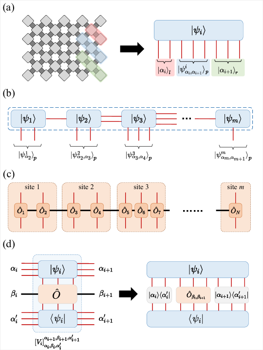
A qMPS is a multi-component structure that represents a large global state through a group of distributed smaller-scale quantum states, as shown in Fig. 1. The -th site of the qMPS is a physical quantum state given by
| (2) |
where qubits are partitioned into three entangled groups labeled (left auxiliary), (physical) and (right auxiliary). A qMPS site is naturally a rank- quantum tensor Yuan et al. (2021), and the elements of this tensor are the amplitudes of this state. For consistency with a MPS with a bond dimension of , we allocate qubits per auxiliary dimension, and there can be totally qubits where is the number of physical qubits used in a qMPS site. Generally , and we focus on cases where to maintain consistency with the classical cases. The data in this site consist of its amplitudes and can be indexed by projecting the state onto the corresponding basis. The space complexity of qMPS naturally scales logarithmically compared to classical MPS.
Contracting two qMPS sites follows the rules Yuan et al. (2021) of
| (3) |
and these qMPS sites form a global -qubit state represented by
| (4) |
also as shown in Fig. 1(b). The number of qubits in the global state is the sum of qubits in the physical dimension of each qMPS site. The auxiliary dimension, if not bounded, grows exponentially within a classical MPS, while the number of auxiliary qubits grows linearly. Therefore, the qMPS model can be used for strongly entangled systems.
Calculating the global expectation of a qMPS over a global observable can be done locally. In the language of MPS, the observable can first be decomposed into the form of matrix product operator (MPO), and the corresponding physical dimensions are divided into groups in correspondence to every qMPS site. For any -qubit observable, it can be written as the sum of Pauli products where , and further in a diagonalized MPO form
| (5) | ||||
Note that the multiplications between Pauli operators are tensor products. Practically, we only need to record the appearance of each Pauli operator instead of storing every whole MPO site. For simplicity, the coefficients for each term is concentrated in . These MPO sites can be divided into groups to match the number of physical qubits in each qMPS site, as shown in Fig. 1(c).
The calculation of expectation can be done locally on quantum devices, as shown in Fig. 1(d). Suppose we are now at site of the qMPS, which is in state . The corresponding MPO site is represented by where and are the physical dimensions. For a MPO generated following Eq. 5, it satisfies that given , and thus is compatible with quantum measurement. The result of the local expectation is therefore a sparse rank-6 classical tensor
| (6) |
This can be done by measuring by expanding every and into series of Pauli terms Yuan et al. (2021). Running over , , and for each connecting qubits and leading to a time complexity of for a single term. The global expectation value can be calculated by classical tensor contraction, and the overall complexity to evaluate the global expectation is , where is the number of terms in the global observable, and is the number of qMPS sites.
III Turning a qMPS into canonical form
An important step before applying MPS is to turn it into canonical form. For example, Eq. 7 (8) shows how a MPS site is in right(left)-canonical form.
| (7) |
| (8) |
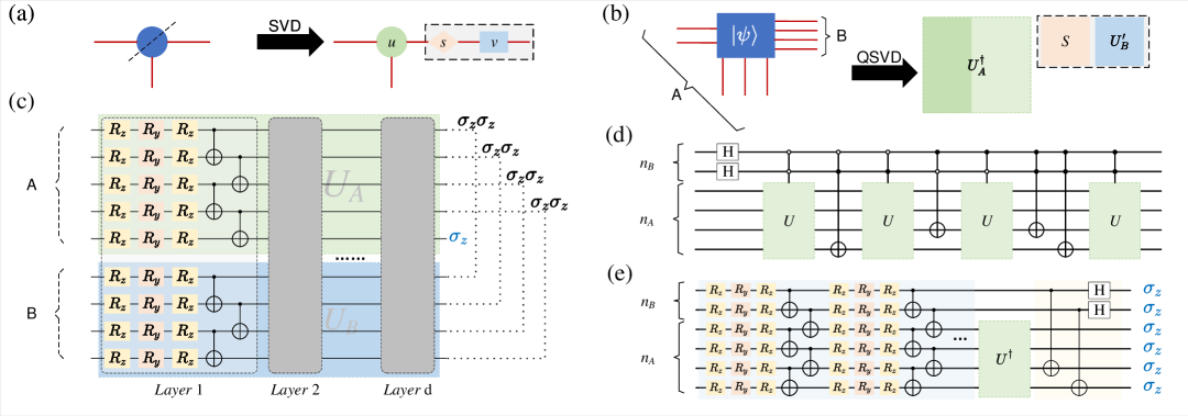
where indicates to take the elementwise conjugate of the tensor . For classical MPS, this is done by Singular value decomposition (SVD). Unlike ref. Schuhmacher et al. (2025) that uses classical ancillary data, here we apply quantum algorhms to turn a qMPS site into canonical form, through quantum singular value decomposition (QSVD) and a quantum reshape algorithm, as shown in Fig. 2.
III.1 Quantum SVD for imbalanced system
The system is divided into two subsystems, and the main idea for decomposing a state is to find two unitaries and for diagonalization, such that , as shown in Fig. 2(b) Bravo-Prieto et al. (2020). This is done through a variational algorithm optimizing . We note that another variational method exists for decomposing a unitary matrix Wang et al. (2021), but in qMPS, it has to deal with a state rather than a matrix, and we have to extend the method for imbalanced systems where the number of qubits in the subsystems is unequal. Specifically for such a system, the loss function must also account for the remaining qubits, which can be updated as
| (9) |
where ‘’ denotes the set of the remaining qubits except those in the correlated measurements. We construct a variational circuit for this purpose as shown in Fig. 2(c). Without loss of generality, we assume . The circuit is divided into two parts, containing and qubits respectively. In each layer of the circuit, it comprises single-qubit rotations and interlacing CNOT gates. The decomposition requires that if subsystem is measured as (in the binary representation of its qubits), then subsystem should also be in state (in the binary representation of its qubits). This is done through the correlate measurement on the overlapped qubits of the two subsystems through the observable of , meanwhile the rest qubits are measured in basis. Optimization is performed using standard variational algorithms, by gradient descent method. The two unitaries are obtained when the loss is optimized to zero, yielding the decomposition as
| (10) | ||||
where and is the conjugate of . As shown in Ref. Bravo-Prieto et al. (2020), the loss decays exponentially fast when the depth of the circuit grows.
III.2 Quantum reshape
To convert a qMPS site into canonical form, one should transfer the result of QSVD (i.e., or ) into a qMPS site (i.e., a quantum state), and apply the other unitary as well as the diagonal matrix of singular values to the neighbouring site. For the first step, we employ a quantum reshape algorithm. The corresponding circuit to implement this is straight forward, as shown in Fig. 2(d). To prepare a left-canonical site, we directly apply in this circuit, and it will concatenate the columns of into a state vector
| (11) |
However, this circuit may be too deep for near-term devices, and we also develop a variational algorithm for this reshape, as shown in Fig. 2(e). The idea for this is to approximate with a variational circuit. Applying to the latter part of the state produces a maximally entangled state, and can further be transformed into using merely CNOT and Hadamard gates. The corresponding cost function is
| (12) |
If is optimized to 0, the output state can be determined to be and the variational circuit produces shown in eq. 11 ideally. In our numerical simulations, we find that the variational reshape can achieve fidelities exceeding for circuits with 7 qubits. To prepare a right-canonical site, the corresponding data (the rows of ) can be obtained similarly.
The latter step is to keep the global state invariant by merging the rest result of QSVD (that is or ) to the neighbouring site. We can also apply another variational algorithm to find the result of applying this operation on the neighbouring site Motta et al. (2020), but fortunately, in some cases this step is unnecessary, such as in the variational qMPS (vqMPS) method we will introduce in the next section.
IV The variational MPS method on a quantum computer
Perhaps the most important application of MPS is the variational MPS (vMPS) method for finding ground energy of many-body system, which is equivalent to the DMRG method White (1992); Schollwöck (2005). With qMPS and all the components mentioned above, we can run this algorithm on quantum devices, and we denote this method by variatioanl quantum MPS (vqMPS) method. The vMPS algorithm updates the tensors site-by-site (or more than one site at a time) instead of optimizing the whole system. For site , the other qMPS sites and the Hamiltonian MPO constitute its environment, or more specifically the effective Hamiltonian. This site then can be updated by the ground state of the effective Hamiltonian (see Ref. Schollwöck (2005, 2011) for detials). The vqMPS procedure closely resembles classical vMPS, by performing back-and-forth sweeps, as shown in Fig. 3.

The global qMPS is prepared randomly with separate quantum states, and turned into left-canonical form for sweeping from right to left. For each site, the number of qubits is determined according to the size of bond dimensions. During a sweeping process, the states are updated site-by-site, through finding the ground state of the effective Hamiltonian.
Consider updating site during a sweep from right to left, the effective hamiltonian is constructed by contracting the local tensors obtained following Eq. 6, as shown in Eq. 13.
| (13) |
where means the contraction of all tensors with connected dimensions. We then find the ground state of through quantum algorithms like VQE or perhaps the quantum phase estimation algorithm in the future which can bring quantum advantages. The energy obtained during sweeps corresponds to the expectation value of the updated qMPS with respect to the global Hamiltonian. The number of qubits involved in this step is . This state is then decomposed as through the method mentioned above. This site can then be updated through reshaped . Since we are going to update the -th site, are no longer necessary to merge.
In practice, vqMPS can adopt a hybrid computing paradigm: Sites near boundaries with low entanglement can be efficiently updated using classical DMRG on classical computers, while central sites exhibiting strong entanglement reside on quantum devices. Consequently, this strategy leverages the advantages of both classical and quantum computing and avoids frequent quantum-classical interactions appearing in conventional VQE.
V Numerical simulation
We conduct the numerical simulation to demonstrate vqMPS on a personal computer to show evidence for quantum devices to run tensor network algorithms.
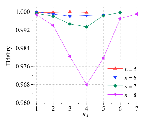
We first demonstrate the quantum SVD method for imbalanced systems. As a proof of principle, Fig. 4 shows the numerical results of decomposing random states. The circuits used are in consistency with those shown in Fig. 2(c). The result of the decomposition can be validated through the fidelity of the recovered state with the original state. We test to decompose states containing to qubits. For each case, we first decompose it to qubits using a variational circuit with sufficient depth, then calculate the fidelity between the original state and the state recovered from the learned parameters. Each point is averaged through 3 tests. The recovered state can reach identity fidelities for and , and the results for more qubits are shown in Fig. 4. All results reaches fidelity higher than 96%.
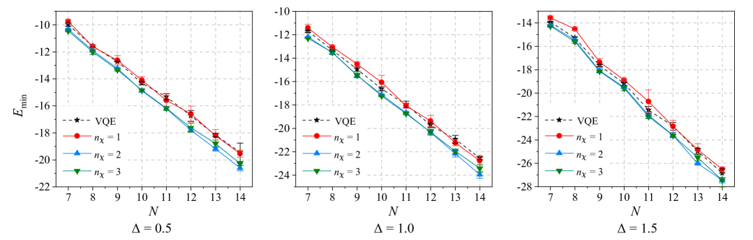
We demonstrate the vqMPS method for finding the ground energy of Heisenberg XXZ spin-chain model
| (14) |
where is set to be , and , respectively. We test vqMPS method with bond dimensions fixed at or , corresponding to using or ancillary qubits. The structure of the variational circuits are similar to that used in Fig. 2(c) but the depth of the circuit is limited to for -qubit VQE. The results are shown in Fig. 5.
We performed 300 iterations and reached a good convergence for each optimization process. The maximum number of iterations is limited to control the computing cost. Since the depth of the circuits as well as the number of iterations are limited, the optimization process may not reach the ground truth. But in vqMPS, the VQE can reach a much higher ratio towards the optimal value owing to the reduced number of qubits. For VQE with less than 5 qubits, using such configurations can reach nearly optimal values, but for VQE with a large number of qubits, it requires both longer time for each step and more steps to converge. The vqMPS method can be scaled up to tens of qubits, and the time complexity is approximately linear. For all the cases, we find the vqMPS can reach a comparable accuracy compared with VQE when using merely qubit for connecting (i.e. ), namely each local optimization by VQE involves at most 3 qubits. The accuracy can be further improved for and , using 5 or 7-qubit VQE. For some cases using can be less accurate compared with that of , again reflecting the difficulty in large-scale VQE.
VI Conclusion
In this paper, we propose the qMPS model and the variational qMPS method, which is actually the quantum version of the DMRG method. We update the quantum methods for preparing a qMPS in the canonical form. The whole method can be done on quantum devices and we demonstrate this method through numerical simulation. The state is updated locally, and therefore can greatly reduce the number of qubits involved in variational algorithms, while maintaining the accuracy. For qMPS, the auxiliary dimensions are represented by qubits, and can bring in logarithmic space complexity in storing tensor data. However, the result is strongly correlated with the quality of the optimization, including the procedures of QSVD and the VQE. It is worthy pointing out that for state with concentrated spectrum, the fidelity of the recovered state from the decomposed results can be nearly identity, but the base vectors learned corresponding to small singular values can be biased. The accuracy of vqMPS can be further improved using deterministic algorithms on quantum devices with error corrections. These models and methods show the possibilities of transplanting efficient classical algorithms to quantum devices, as well as the means for quantum-classical hybrid tasks.
Acknowledgements.
We appreciate the helpful discussion with other members of the QUANTA group. This work was funded by the National Key R&D Program of China under Grant No. 2024YFB4504001, the National Natural Science Foundation of China under Grant No. 62401572, the Aid Program for Science and Technology Innovative Research Team in Higher Educational Institutions of Hunan Province, and the Open Research Fund from State Key Laboratory of High Performance Computing of China under Grant No. 202401-06.References
- Feynman (1982) R. P. Feynman, International journal of theoretical physics 21, 467 (1982).
- Anderson (1984) P. W. Anderson, Basic notions of condensed matter physics (Benjamin/Cummings, 1984).
- Sachdev (2023) S. Sachdev, Quantum Phases of Matter (Cambridge University Press, 2023).
- Cao et al. (2019) Y. Cao, J. Romero, J. P. Olson, M. Degroote, P. D. Johnson, M. Kieferová, I. D. Kivlichan, T. Menke, B. Peropadre, N. P. D. Sawaya, S. Sim, L. Veis, and A. Aspuru-Guzik, Chemical Reviews 119, 10856 (2019).
- McArdle et al. (2020) S. McArdle, S. Endo, A. Aspuru-Guzik, S. C. Benjamin, and X. Yuan, Rev. Mod. Phys. 92, 015003 (2020).
- Zohar et al. (2015) E. Zohar, J. I. Cirac, and B. Reznik, Reports on Progress in Physics 79, 014401 (2015).
- Martinez et al. (2016) E. A. Martinez, C. A. Muschik, P. Schindler, D. Nigg, A. Erhard, M. Heyl, P. Hauke, M. Dalmonte, T. Monz, P. Zoller, and R. Blatt, Nature 534, 516 (2016).
- Monroe et al. (2021) C. Monroe, W. C. Campbell, L.-M. Duan, Z.-X. Gong, A. V. Gorshkov, P. W. Hess, R. Islam, K. Kim, N. M. Linke, G. Pagano, P. Richerme, C. Senko, and N. Y. Yao, Rev. Mod. Phys. 93, 025001 (2021).
- Maskara et al. (2025) N. Maskara, S. Ostermann, J. Shee, M. Kalinowski, A. McClain Gomez, R. Araiza Bravo, D. S. Wang, A. I. Krylov, N. Y. Yao, M. Head-Gordon, M. D. Lukin, and S. F. Yelin, Nature Physics 21, 289 (2025).
- Wong et al. (2023) Y. K. Wong, Y. Zhou, Y. S. Liang, H. Qiu, Y. X. Wu, and B. He, in 2023 IEEE 4th International Conference on Pattern Recognition and Machine Learning (PRML) (2023) pp. 557–564.
- Santagati et al. (2024) R. Santagati, A. Aspuru-Guzik, R. Babbush, M. Degroote, L. González, E. Kyoseva, N. Moll, M. Oppel, R. M. Parrish, N. C. Rubin, M. Streif, C. S. Tautermann, H. Weiss, N. Wiebe, and C. Utschig-Utschig, Nature Physics 20, 549 (2024).
- Moll et al. (2018) N. Moll, P. Barkoutsos, L. S. Bishop, J. M. Chow, A. Cross, D. J. Egger, S. Filipp, A. Fuhrer, J. M. Gambetta, M. Ganzhorn, A. Kandala, A. Mezzacapo, P. Müller, W. Riess, G. Salis, J. Smolin, I. Tavernelli, and K. Temme, Quantum Science and Technology 3, 030503 (2018).
- Harrigan et al. (2021) M. P. Harrigan, K. J. Sung, M. Neeley, K. J. Satzinger, F. Arute, K. Arya, J. Atalaya, J. C. Bardin, R. Barends, S. Boixo, M. Broughton, B. B. Buckley, D. A. Buell, B. Burkett, N. Bushnell, Y. Chen, Z. Chen, B. Chiaro, R. Collins, W. Courtney, S. Demura, A. Dunsworth, D. Eppens, A. Fowler, B. Foxen, C. Gidney, M. Giustina, R. Graff, S. Habegger, A. Ho, S. Hong, T. Huang, L. B. Ioffe, S. V. Isakov, E. Jeffrey, Z. Jiang, C. Jones, D. Kafri, K. Kechedzhi, J. Kelly, S. Kim, P. V. Klimov, A. N. Korotkov, F. Kostritsa, D. Landhuis, P. Laptev, M. Lindmark, M. Leib, O. Martin, J. M. Martinis, J. R. McClean, M. McEwen, A. Megrant, X. Mi, M. Mohseni, W. Mruczkiewicz, J. Mutus, O. Naaman, C. Neill, F. Neukart, M. Y. Niu, T. E. O’Brien, B. O’Gorman, E. Ostby, A. Petukhov, H. Putterman, C. Quintana, P. Roushan, N. C. Rubin, D. Sank, A. Skolik, V. Smelyanskiy, D. Strain, M. Streif, M. Szalay, A. Vainsencher, T. White, Z. J. Yao, P. Yeh, A. Zalcman, L. Zhou, H. Neven, D. Bacon, E. Lucero, E. Farhi, and R. Babbush, Nature Physics 17, 332 (2021).
- Arute et al. (2019) F. Arute, K. Arya, R. Babbush, D. Bacon, J. C. Bardin, R. Barends, R. Biswas, S. Boixo, F. G. S. L. Brandao, D. A. Buell, B. Burkett, Y. Chen, Z. Chen, B. Chiaro, R. Collins, W. Courtney, A. Dunsworth, E. Farhi, B. Foxen, A. Fowler, C. Gidney, M. Giustina, R. Graff, K. Guerin, S. Habegger, M. P. Harrigan, M. J. Hartmann, A. Ho, M. Hoffmann, T. Huang, T. S. Humble, S. V. Isakov, E. Jeffrey, Z. Jiang, D. Kafri, K. Kechedzhi, J. Kelly, P. V. Klimov, S. Knysh, A. Korotkov, F. Kostritsa, D. Landhuis, M. Lindmark, E. Lucero, D. Lyakh, S. Mandrà, J. R. McClean, M. McEwen, A. Megrant, X. Mi, K. Michielsen, M. Mohseni, J. Mutus, O. Naaman, M. Neeley, C. Neill, M. Y. Niu, E. Ostby, A. Petukhov, J. C. Platt, C. Quintana, E. G. Rieffel, P. Roushan, N. C. Rubin, D. Sank, K. J. Satzinger, V. Smelyanskiy, K. J. Sung, M. D. Trevithick, A. Vainsencher, B. Villalonga, T. White, Z. J. Yao, P. Yeh, A. Zalcman, H. Neven, and J. M. Martinis, Nature 574, 505 (2019).
- Zhu et al. (2022) Q. Zhu, S. Cao, F. Chen, M.-C. Chen, X. Chen, T.-H. Chung, H. Deng, Y. Du, D. Fan, M. Gong, C. Guo, C. Guo, S. Guo, L. Han, L. Hong, H.-L. Huang, Y.-H. Huo, L. Li, N. Li, S. Li, Y. Li, F. Liang, C. Lin, J. Lin, H. Qian, D. Qiao, H. Rong, H. Su, L. Sun, L. Wang, S. Wang, D. Wu, Y. Wu, Y. Xu, K. Yan, W. Yang, Y. Yang, Y. Ye, J. Yin, C. Ying, J. Yu, C. Zha, C. Zhang, H. Zhang, K. Zhang, Y. Zhang, H. Zhao, Y. Zhao, L. Zhou, C.-Y. Lu, C.-Z. Peng, X. Zhu, and J.-W. Pan, Science Bulletin 67, 240 (2022).
- Madsen et al. (2022) L. S. Madsen, F. Laudenbach, M. F. Askarani, F. Rortais, T. Vincent, J. F. F. Bulmer, F. M. Miatto, L. Neuhaus, L. G. Helt, M. J. Collins, A. E. Lita, T. Gerrits, S. W. Nam, V. D. Vaidya, M. Menotti, I. Dhand, Z. Vernon, N. Quesada, and J. Lavoie, Nature 606, 75 (2022).
- Zhong et al. (2021) H.-S. Zhong, Y.-H. Deng, J. Qin, H. Wang, M.-C. Chen, L.-C. Peng, Y.-H. Luo, D. Wu, S.-Q. Gong, H. Su, Y. Hu, P. Hu, X.-Y. Yang, W.-J. Zhang, H. Li, Y. Li, X. Jiang, L. Gan, G. Yang, L. You, Z. Wang, L. Li, N.-L. Liu, J. J. Renema, C.-Y. Lu, and J.-W. Pan, Phys. Rev. Lett. 127, 180502 (2021).
- Deng et al. (2023) Y.-H. Deng, Y.-C. Gu, H.-L. Liu, S.-Q. Gong, H. Su, Z.-J. Zhang, H.-Y. Tang, M.-H. Jia, J.-M. Xu, M.-C. Chen, J. Qin, L.-C. Peng, J. Yan, Y. Hu, J. Huang, H. Li, Y. Li, Y. Chen, X. Jiang, L. Gan, G. Yang, L. You, L. Li, H.-S. Zhong, H. Wang, N.-L. Liu, J. J. Renema, C.-Y. Lu, and J.-W. Pan, Phys. Rev. Lett. 131, 150601 (2023).
- Acharya et al. (2025) R. Acharya, D. A. Abanin, L. Aghababaie-Beni, I. Aleiner, T. I. Andersen, M. Ansmann, F. Arute, K. Arya, A. Asfaw, N. Astrakhantsev, J. Atalaya, R. Babbush, D. Bacon, B. Ballard, J. C. Bardin, J. Bausch, A. Bengtsson, A. Bilmes, S. Blackwell, S. Boixo, G. Bortoli, A. Bourassa, J. Bovaird, L. Brill, M. Broughton, D. A. Browne, B. Buchea, B. B. Buckley, D. A. Buell, T. Burger, B. Burkett, N. Bushnell, A. Cabrera, J. Campero, H.-S. Chang, Y. Chen, Z. Chen, B. Chiaro, D. Chik, C. Chou, J. Claes, A. Y. Cleland, J. Cogan, R. Collins, P. Conner, W. Courtney, A. L. Crook, B. Curtin, S. Das, A. Davies, L. De Lorenzo, D. M. Debroy, S. Demura, M. Devoret, A. Di Paolo, P. Donohoe, I. Drozdov, A. Dunsworth, C. Earle, T. Edlich, A. Eickbusch, A. M. Elbag, M. Elzouka, C. Erickson, L. Faoro, E. Farhi, V. S. Ferreira, L. F. Burgos, E. Forati, A. G. Fowler, B. Foxen, S. Ganjam, G. Garcia, R. Gasca, É. Genois, W. Giang, C. Gidney, D. Gilboa, R. Gosula, A. G. Dau, D. Graumann, A. Greene, J. A. Gross, S. Habegger, J. Hall, M. C. Hamilton, M. Hansen, M. P. Harrigan, S. D. Harrington, F. J. H. Heras, S. Heslin, P. Heu, O. Higgott, G. Hill, J. Hilton, G. Holland, S. Hong, H.-Y. Huang, A. Huff, W. J. Huggins, L. B. Ioffe, S. V. Isakov, J. Iveland, E. Jeffrey, Z. Jiang, C. Jones, S. Jordan, C. Joshi, P. Juhas, D. Kafri, H. Kang, A. H. Karamlou, K. Kechedzhi, J. Kelly, T. Khaire, T. Khattar, M. Khezri, S. Kim, P. V. Klimov, A. R. Klots, B. Kobrin, P. Kohli, A. N. Korotkov, F. Kostritsa, R. Kothari, B. Kozlovskii, J. M. Kreikebaum, V. D. Kurilovich, N. Lacroix, D. Landhuis, T. Lange-Dei, B. W. Langley, P. Laptev, K.-M. Lau, L. Le Guevel, J. Ledford, J. Lee, K. Lee, Y. D. Lensky, S. Leon, B. J. Lester, W. Y. Li, Y. Li, A. T. Lill, W. Liu, W. P. Livingston, A. Locharla, E. Lucero, D. Lundahl, A. Lunt, S. Madhuk, F. D. Malone, A. Maloney, S. Mandrà, J. Manyika, L. S. Martin, O. Martin, S. Martin, C. Maxfield, J. R. McClean, M. McEwen, S. Meeks, A. Megrant, X. Mi, K. C. Miao, A. Mieszala, R. Molavi, S. Molina, S. Montazeri, A. Morvan, R. Movassagh, W. Mruczkiewicz, O. Naaman, M. Neeley, C. Neill, A. Nersisyan, H. Neven, M. Newman, J. H. Ng, A. Nguyen, M. Nguyen, C.-H. Ni, M. Y. Niu, T. E. O’Brien, W. D. Oliver, A. Opremcak, K. Ottosson, A. Petukhov, A. Pizzuto, J. Platt, R. Potter, O. Pritchard, L. P. Pryadko, C. Quintana, G. Ramachandran, M. J. Reagor, J. Redding, D. M. Rhodes, G. Roberts, E. Rosenberg, E. Rosenfeld, P. Roushan, N. C. Rubin, N. Saei, D. Sank, K. Sankaragomathi, K. J. Satzinger, H. F. Schurkus, C. Schuster, A. W. Senior, M. J. Shearn, A. Shorter, N. Shutty, V. Shvarts, S. Singh, V. Sivak, J. Skruzny, S. Small, V. Smelyanskiy, W. C. Smith, R. D. Somma, S. Springer, G. Sterling, D. Strain, J. Suchard, A. Szasz, A. Sztein, D. Thor, A. Torres, M. M. Torunbalci, A. Vaishnav, J. Vargas, S. Vdovichev, G. Vidal, B. Villalonga, C. V. Heidweiller, S. Waltman, S. X. Wang, B. Ware, K. Weber, T. Weidel, T. White, K. Wong, B. W. K. Woo, C. Xing, Z. J. Yao, P. Yeh, B. Ying, J. Yoo, N. Yosri, G. Young, A. Zalcman, Y. Zhang, N. Zhu, N. Zobrist, G. Q. AI, and Collaborators, Nature 638, 920 (2025).
- Gao et al. (2025) D. Gao, D. Fan, C. Zha, J. Bei, G. Cai, J. Cai, S. Cao, F. Chen, J. Chen, K. Chen, X. Chen, X. Chen, Z. Chen, Z. Chen, Z. Chen, W. Chu, H. Deng, Z. Deng, P. Ding, X. Ding, Z. Ding, S. Dong, Y. Dong, B. Fan, Y. Fu, S. Gao, L. Ge, M. Gong, J. Gui, C. Guo, S. Guo, X. Guo, L. Han, T. He, L. Hong, Y. Hu, H.-L. Huang, Y.-H. Huo, T. Jiang, Z. Jiang, H. Jin, Y. Leng, D. Li, D. Li, F. Li, J. Li, J. Li, J. Li, J. Li, N. Li, S. Li, W. Li, Y. Li, Y. Li, F. Liang, X. Liang, N. Liao, J. Lin, W. Lin, D. Liu, H. Liu, M. Liu, X. Liu, X. Liu, Y. Liu, H. Lou, Y. Ma, L. Meng, H. Mou, K. Nan, B. Nie, M. Nie, J. Ning, L. Niu, W. Peng, H. Qian, H. Rong, T. Rong, H. Shen, Q. Shen, H. Su, F. Su, C. Sun, L. Sun, T. Sun, Y. Sun, Y. Tan, J. Tan, L. Tang, W. Tu, C. Wan, J. Wang, B. Wang, C. Wang, C. Wang, C. Wang, J. Wang, L. Wang, R. Wang, S. Wang, X. Wang, X. Wang, X. Wang, Y. Wang, Z. Wei, J. Wei, D. Wu, G. Wu, J. Wu, S. Wu, Y. Wu, S. Xie, L. Xin, Y. Xu, C. Xue, K. Yan, W. Yang, X. Yang, Y. Yang, Y. Ye, Z. Ye, C. Ying, J. Yu, Q. Yu, W. Yu, X. Zeng, S. Zhan, F. Zhang, H. Zhang, K. Zhang, P. Zhang, W. Zhang, Y. Zhang, Y. Zhang, L. Zhang, G. Zhao, P. Zhao, X. Zhao, X. Zhao, Y. Zhao, Z. Zhao, L. Zheng, F. Zhou, L. Zhou, N. Zhou, N. Zhou, S. Zhou, S. Zhou, Z. Zhou, C. Zhu, Q. Zhu, G. Zou, H. Zou, Q. Zhang, C.-Y. Lu, C.-Z. Peng, X. Zhu, and J.-W. Pan, Phys. Rev. Lett. 134, 090601 (2025).
- Preskill (2018) J. Preskill, Quantum (2018).
- Peruzzo et al. (2014) A. Peruzzo, J. McClean, P. Shadbolt, M.-H. Yung, X.-Q. Zhou, P. J. Love, A. Aspuru-Guzik, and J. L. O’Brien, Nature Communications 5, 4213 (2014).
- Kandala et al. (2017) A. Kandala, A. Mezzacapo, K. Temme, M. Takita, M. Brink, J. M. Chow, and J. M. Gambetta, Nature 549, 242 (2017).
- Liu et al. (2022) Z. Liu, L.-W. Yu, L.-M. Duan, and D.-L. Deng, Phys. Rev. Lett. 129, 270501 (2022).
- Wang et al. (2021) X. Wang, Z. Song, and Y. Wang, Quantum 5, 483 (2021).
- Peng et al. (2020) T. Peng, A. W. Harrow, M. Ozols, and X. Wu, Phys. Rev. Lett. 125, 150504 (2020).
- Tang and Martonosi (2022) W. Tang and M. Martonosi, “Cutting quantum circuits to run on quantum and classical platforms,” (2022), arXiv:2205.05836 [quant-ph] .
- Yuan et al. (2021) X. Yuan, J. Sun, J. Liu, Q. Zhao, and Y. Zhou, Phys. Rev. Lett. 127, 040501 (2021).
- Markov et al. (2018) I. L. Markov, A. Fatima, S. V. Isakov, and S. Boixo, arXiv preprint arXiv:1807.10749 (2018).
- Villalonga et al. (2019) B. Villalonga, S. Boixo, B. Nelson, C. Henze, E. Rieffel, R. Biswas, and S. Mandrà, npj Quantum Information 5, 86 (2019).
- Villalonga et al. (2020) B. Villalonga, D. Lyakh, S. Boixo, H. Neven, T. S. Humble, R. Biswas, E. G. Rieffel, A. Ho, and S. Mandrà, Quantum Science and Technology 5, 034003 (2020).
- Guo et al. (2019) C. Guo, Y. Liu, M. Xiong, S. Xue, X. Fu, A. Huang, X. Qiang, P. Xu, J. Liu, S. Zheng, H.-L. Huang, M. Deng, D. Poletti, W.-S. Bao, and J. Wu, Physical Review Letters 123, 190501 (2019).
- Liu et al. (2021) Y. Liu, X. Liu, F. Li, H. Fu, Y. Yang, J. Song, P. Zhao, Z. Wang, D. Peng, H. Chen, C. Guo, H. Huang, W. Wu, and D. Chen, in SC21: International Conference for High Performance Computing, Networking, Storage and Analysis (2021) pp. 1–12.
- Pan et al. (2022) F. Pan, K. Chen, and P. Zhang, Phys. Rev. Lett. 129, 090502 (2022).
- Östlund and Rommer (1995) S. Östlund and S. Rommer, Phys. Rev. Lett. 75, 3537 (1995).
- Hastings (2007) M. B. Hastings, Journal of Statistical Mechanics: Theory and Experiment 2007, P08024 (2007).
- Liu et al. (2020) Y. Liu, D. Wang, S. Xue, A. Huang, X. Fu, X. Qiang, P. Xu, H.-L. Huang, M. Deng, C. Guo, X. Yang, and J. Wu, Phys. Rev. A 101, 052316 (2020).
- White (1992) S. R. White, Phys. Rev. Lett. 69, 2863 (1992).
- Schollwöck (2011) U. Schollwöck, Annals of Physics 326, 96 (2011), january 2011 Special Issue.
- Schuhmacher et al. (2025) J. Schuhmacher, M. Ballarin, A. Baiardi, G. Magnifico, F. Tacchino, S. Montangero, and I. Tavernelli, PRX Quantum 6, 010320 (2025).
- Bravo-Prieto et al. (2020) C. Bravo-Prieto, D. García-Martín, and J. I. Latorre, Phys. Rev. A 101, 062310 (2020).
- Motta et al. (2020) M. Motta, C. Sun, A. T. K. Tan, M. J. O’Rourke, E. Ye, A. J. Minnich, F. G. S. L. Brandão, and G. K.-L. Chan, Nature Physics 16, 205 (2020).
- Schollwöck (2005) U. Schollwöck, Rev. Mod. Phys. 77, 259 (2005).