Submillimeter and Mid-Infrared Variability of Young Stellar Objects in the M 17 H II Region

Abstract

We conducted a comprehensive analysis of young stellar object (YSO) variability at submillimeter and mid-infrared (mid-IR) wavelengths for the M 17 H II region, using 3.5 years monitoring data from the JCMT Transient Survey at $450$ and $850\,\mu$m and 9 years mid-IR monitoring data from the NEOWISE mission. Our study encompasses observations of 198 and 164 bright submillimeter peaks identified within the deep JCMT coadded maps at 450 and $850\,\mu$m, and 66 YSOs seen by NEOWISE W2 that were previously identified in mid-IR observations. We find one robust linear submillimeter variable, an intermediate mass protostar, with a $4\%$ peak flux change in 3.5 years of JCMT monitoring that sets a lower limit of $16\%$ luminosity increase for the source. At mid-IR wavelengths, our analysis reveals secular and stochastic variability in 22 YSOs, with the highest fraction of secular variability occurring at the earliest evolutionary stage. This mid-IR fractional variability as a function of evolutionary stage result is similar to what has previously been found for YSO variability within the Gould Belt and the intermediate-mass star formation region M17 SWex, though overall less variability is detected in M 17 in submillimeter and mid-IR. We suspect that this lower detection of YSO variability is due to both the greater distance to M 17 and the strong feedback from the H II region. Our findings showcase the utility of multiwavelength observations to better capture the complex variability phenomena inherent to star formation processes and demonstrate the importance of years-long monitoring of a diverse selection of star-forming environments.

1 Introduction

Episodic accretion events of low-mass young stellar objects (YSOs) have been observed for decades, primarily through optical outbursts (see review by Audard et al., 2014; Fischer et al., 2023). Recent discoveries at longer wavelengths have included YSO bursts at younger stages of protostellar evolution (Kóspál et al., 2007; Megeath et al., 2012; Safron et al., 2015; Contreras Peña et al., 2017; Hodapp et al., 2019; Park et al., 2021; Lee et al., 2021), closer to the peak time of the stellar mass assembly. However, only a few bursts have been identified from massive YSOs, usually uncovered by monitoring maser emission with confirmation through infrared follow-up observations (Caratti o Garatti et al., 2017; Burns et al., 2020; Stecklum et al., 2021; Burns et al., 2023).

In the earliest stages of star formation, numerical simulations predict that episodic accretion bursts might contribute a substantial part to the final stellar mass (e.g. Vorobyov & Basu, 2015; Meyer et al., 2019). Episodic accretion was proposed by Kenyon et al. (1990) as a solution to the “protostellar luminosity problem” observed in Class I YSOs. At the time, these sources appeared to be underluminous on average compared to expectations based on simple accretion arguments. Updated measurements of protostellar luminosities and lifetimes have modified this historical perspective into the “protostellar luminosity spread problem”, the scatter observed around the best-fit isochrones in pre-main-sequence stellar clusters (Baraffe et al., 2009, 2012; Kunitomo et al., 2017). Time-dependent accretion may naturally explain this wide range of protostellar luminosities that span $3-4$ orders of magnitude (see review by Fischer et al., 2023). The higher frequency of accretion bursts during the earliest stages of YSOs, as indicated by the statistics of variable YSOs in the Gould Belt (Park et al., 2021; Zakri et al., 2022), agrees with the expectation of theoretical models of angular momentum transport in accretion disks (e.g. Bae et al., 2014; Vorobyov & Basu, 2015). However, YSOs in the early stages are still deeply embedded in their nascent, dusty envelopes and are thus too heavily extincted for an accretion burst to be directly observed at optical or near-infrared wavelengths. This radiation, emitted by the deeply embedded YSO, is absorbed by the dense envelope and re-radiated at longer wavelengths, with the emitted spectral energy distribution from the envelope peaking at mid- to far-infrared wavelengths. Subsequent changes in observed flux at these, and longer, wavelengths trace the heating and cooling of the envelope due to the internal accretion-driven luminosity variability (Johnstone et al., 2013; MacFarlane et al., 2019a, b; Baek et al., 2020).

In principle, the best wavelength range to monitor the accretion variability of deeply embedded protostars is 20–200 $\mu$m (MacFarlane et al., 2019a; Fischer et al., 2024), but this window is difficult to access with ground-based telescopes. At longer wavelengths, submillimeter monitoring programs have begun to reveal protostellar variability, although at modest levels (e.g. Lee et al., 2021; Francis et al., 2022; Mairs et al., 2024). At shorter wavelengths, monitoring programs with Spitzer and WISE have detected mid-IR variability of YSOs up to several magnitudes (Mainzer et al., 2011; Scholz et al., 2013; Wolk et al., 2018; Park et al., 2021; Lee et al., 2024). Although mid-IR variability can also be affected by changes in the extinction and geometry of asymmetric disks (e.g. Scholz et al., 2015; Nagel & Bouvier, 2019; Covey et al., 2021), in the few sources monitored for both submillimeter and mid-IR variability, the correlated changes are consistent with expectations of accretion variability (Contreras Peña et al., 2020).

Most previous results focus on nearby low-mass protostars. The variability properties towards the higher mass end are much less explored, with a very limited sample of accretion-bursting MYSOs (e.g. Chen et al., 2021; Wolf et al., 2024). All of these accretion-bursting MYSOs exhibit contemporary variability in infrared and submillimeter luminosity and in maser emission (Caratti o Garatti et al., 2017; Hunter et al., 2017; Liu et al., 2018; Chen et al., 2020; Burns et al., 2020; Stecklum et al., 2021; Hunter et al., 2021; Chen et al., 2021; Hirota et al., 2022). The question remains whether similar accretion-driven luminosity bursts to those seen for lower mass YSOs occur in MYSOs and whether these processes might differ in frequency, amplitude, and duration as a function of protostellar mass (Fischer et al., 2023).

The JCMT Transient survey originally focused exclusively on nearby ($<500$ pc) low-mass star-forming regions and expanded in 2020 to monitor six additional fields towards regions of intermediate- to high-mass star formation (Herczeg et al., 2017; Mairs et al., 2024). These six fields are at distances of a few kiloparsec, at which the JCMT beams at 450 and $850\,\mu$m are still capable of resolving sub-parsec dust condensations. Some of these fields were selected because they had been previously found to host variable YSOs showing evidence of accretion bursts (Liu et al., 2018; Park et al., 2019; Chen et al., 2021; Wenner et al., 2022). Two fields are from the M 17 complex (Nguyen-Luong et al., 2020), the well-known Galactic H II region M 17 (Hoffmeister et al., 2008; Chen et al., 2012; Lim et al., 2020) and the filamentary molecular cloud extended to southwest of the M 17 H II region (M17 SWex; Povich & Whitney, 2010). The analyses of the submillimeter and mid-IR variability of YSOs in M17 SWex are presented in Park et al. (2024).

The trigonometric distance to the maser sources associated with M 17 is $\approx 2.0$ kpc (Xu et al., 2011; Chibueze et al., 2016), which we adopt in this work. This distance is consistent with the distance of $\approx 1.7$ kpc measured from Gaia astrometry (Kuhn et al., 2019; Ma´ız Apellániz et al., 2022; Stoop et al., 2024). Figure 1 shows the SDSS g image of M 17 from the VST Photometric H$\alpha$ Survey of the Southern Galactic Plane and Bulge (VPHAS; Drew et al., 2014). The optically bright nebula outlines the location of the M17 H II region, with two adjacent clouds in the north (M17 North) and southwest (M17 SW) of the nebula. The massive stars are mostly located within the M17 H II region (Hoffmeister et al., 2008), meanwhile the YSOs are more concentrated towards M17 SW and M17 North (Hoffmeister et al., 2008; Povich et al., 2009). Notably, M17 MIR in M17 SW, named due to its visibility only at mid-IR and longer wavelengths, was discovered for its recurrent accretion outbursts (Chen et al., 2021; Zhou et al., 2024). The submillimeter and mid-IR variability of the many other YSOs in M 17 is still unexplored.

The results of the analyses for the submillimeter and mid-IR variability of YSOs in M 17 are presented in this paper. The multi-epoch submillimeter and mid-IR data and ancillary data sets are described in Section 2. The analyses of submillimeter and mid-IR variability of YSOs are presented in Section 3. In Section 4, we focus on the interesting YSOs that are variable at submillimeter or mid-IR wavelengths, and compare the results of M 17 to those of other fields of the JCMT Transient Survey.

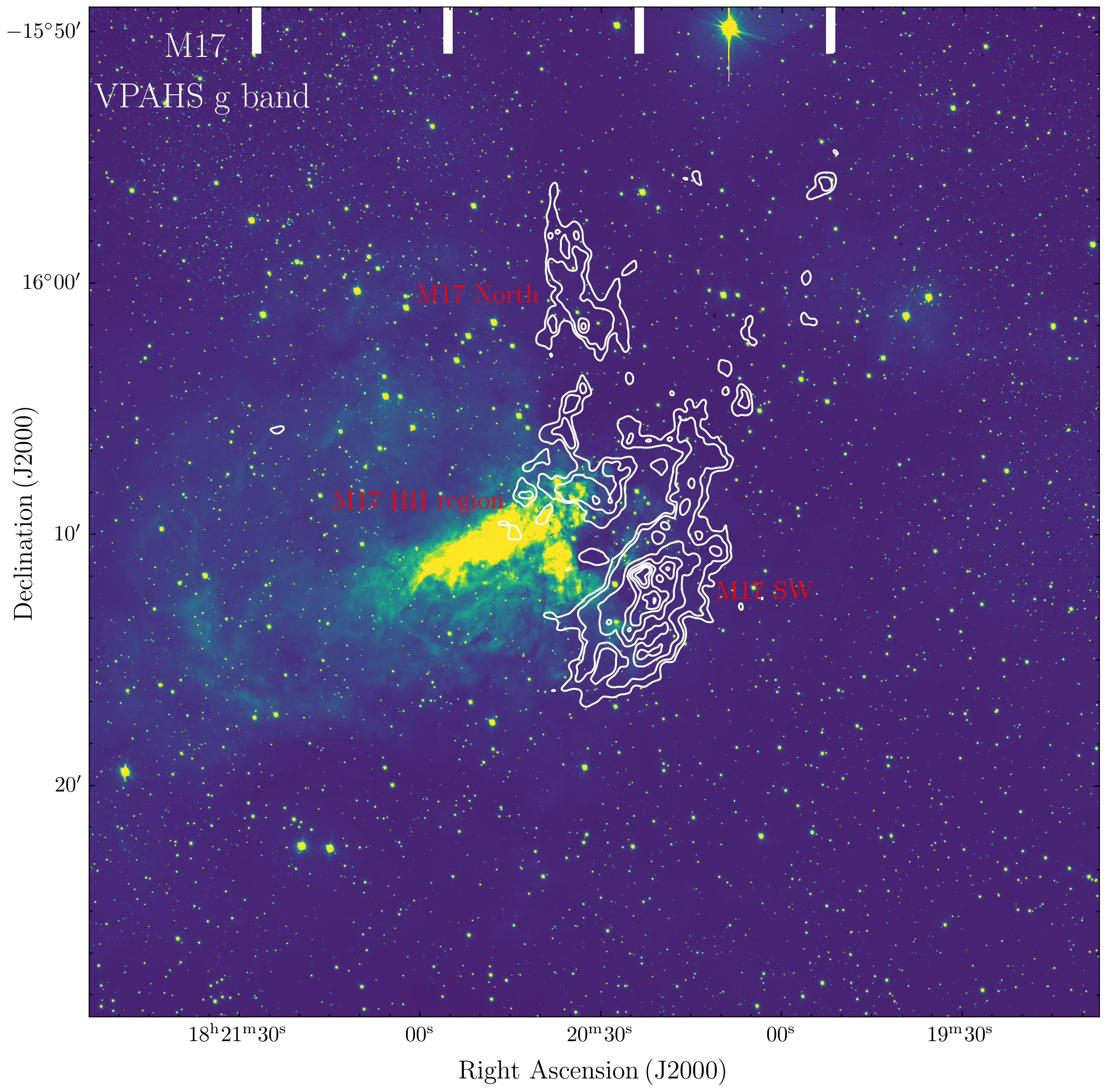
Figure 1: VPAHS $g$-band image of M 17, overlaid with $850\,\mu$m dust continuum contours (in levels 0.3, 0.6, 1.8, 3.6, 6.0, 9.0, 1.26, and 1.68 $\mathrm{Jy\,beam^{-1}}$) from JCMT-SCUBA2. The optically bright nebula in M 17 are labeled as M17 H II region, while the northern and southwestern clouds are labeled as M17 North and M17 SW, respectively.

Table 1: A Summary of JCMT-SCUBA2 Observations at 450 and 850 $\mu$m for M 17

Date	MJD	$\tau\times\mathrm{AM}$	$\mathrm{RMS_{450}}$	$\mathrm{RMS_{850}}$
yyyy-mm-dd			(mJy beam-1)	(mJy beam-1)
2020-02-22	58901.7	0.05	61	9
2020-05-21	58990.5	0.15	-	12
2020-06-23	59023.5	0.14	-	13
2020-07-30	59060.3	0.07	116	11
2020-09-01	59093.2	0.05	44	7
2020-10-10	59132.2	0.17	-	16
2021-03-04	59277.7	0.06	112	11
2021-04-06	59310.6	0.07	86	9
2021-05-17	59351.5	0.06	135	15
2021-06-14	59379.3	0.09	105	9
2021-07-22	59417.4	0.12	-	13
2021-08-22	59448.2	0.12	286	11
2021-09-27	59484.3	0.1	168	10
2021-11-01	59519.2	0.15	-	13
2022-02-19	59629.7	0.07	88	11
2022-05-23	59722.5	0.07	67	8
2022-06-28	59758.4	0.07	106	13
2022-07-29	59789.3	0.1	190	10
2022-08-27	59818.2	0.07	100	10
2022-10-01	59853.3	0.11	275	12
2023-05-01	60065.5	0.16	-	12
2023-06-06	60101.5	0.10	228	11
2023-07-15	60140.3	0.09	201	14
2023-08-12	60168.3	0.06	96	9

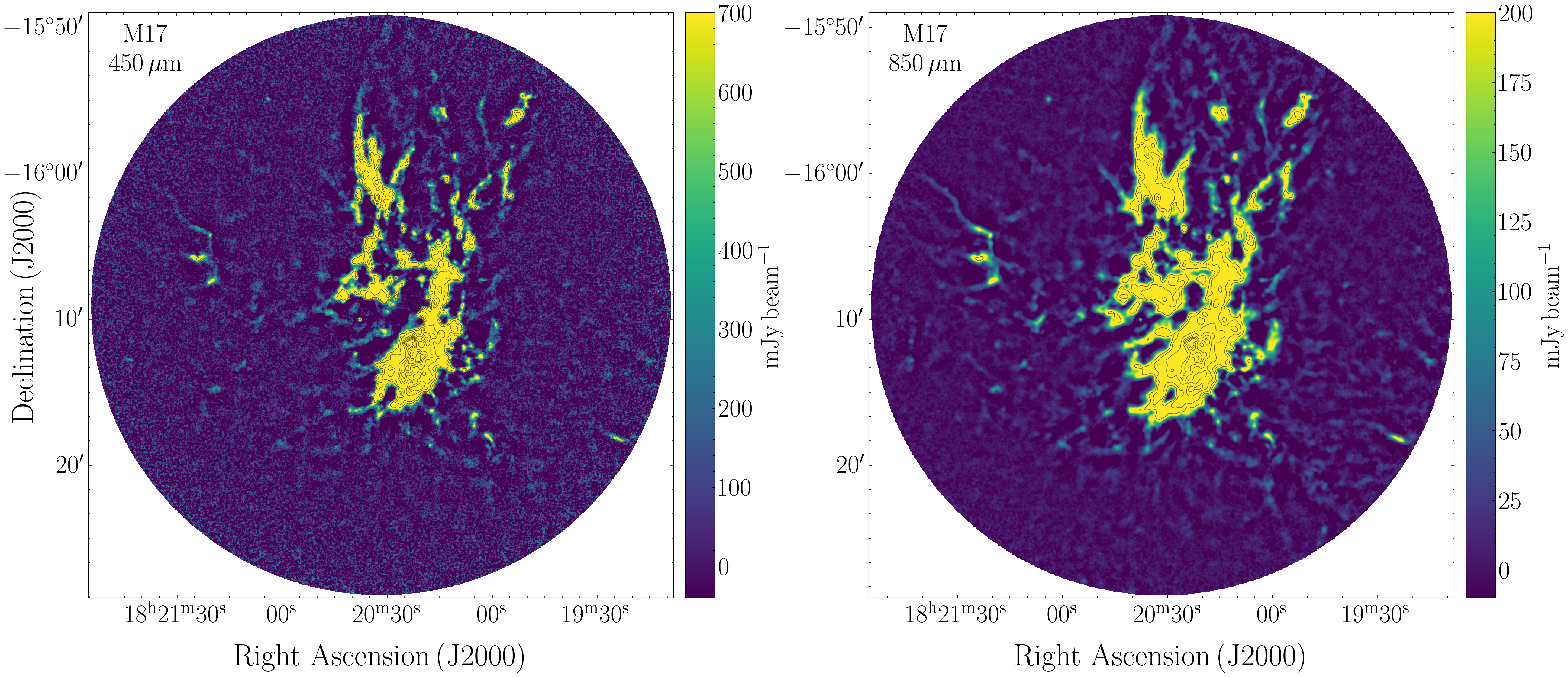
Figure 2: JCMT-SCUBA2 co-added 450 (left) and $850\,\mu$m (right) maps for M 17, overlaid with $450\,\mu$m dust continuum contours (in levels 1, 2, 6, 12, 20, 30, 42, and 56 $\mathrm{Jy\,beam^{-1}}$) and $850\,\mu$m dust continuum contours (in levels 0.3, 0.6, 1.8, 3.6, 6.0, 9.0, 1.26, and 1.68 $\mathrm{Jy\,beam^{-1}}$).

2 Observations and Data

2.1 Submillimeter Data Sets

2.1.1 JCMT Transient Survey

The JCMT Transient survey is designed to measure submillimeter variability of protostars (Herczeg et al., 2017) using the Submillimetre Common User Bolometer Array 2 (SCUBA-2) instrument (Holland et al., 2013) on the James Clerk Maxwell Telescope (JCMT) at the summit of Maunakea, Hawaii. SCUBA-2 observations are performed simultaneously at 450 and $850~\mu$m with effective beam sizes being $10\farcs 0\pm 0\farcs 6$ and $14\farcs 4\pm 0\farcs 3$, or $0.1$ and $0.14$ pc at the distance of M 17, respectively (Kackley et al., 2010; Mairs et al., 2021). Our survey uses the pong $1800\arcsec$ mapping mode, which scans a field of $30\arcmin$ in diameter and produces a uniform background rms noise within the circular field.

SCUBA-2 monitoring observations for M 17 started on February 22, 2020 with a monthly cadence as long as the region is visible by JCMT. During the period from 2020 February to 2023 August, 24 epochs of observations were carried out, although the visit on 28 June 2022 appeared problematic and is excluded from our variability analyses (see Table 1). The $850\,\mu$m data have a consistent background rms noise of $\sim 12\mathrm{mJy\,beam^{-1}}$ for each of these 23 epochs. Observations at $450\,\mu$m strongly depend on atmospheric transmission (Mairs et al., 2024). In 17 of the 23 epochs, the $450\,\mu$m data were obtained with $\tau~\times~\mathrm{airmass}\leqslant 0.12$ and therefore have a low enough rms for variability analysis.

The data reduction procedure was performed using the iterative map making technique MAKEMAP (Chapin et al., 2013) in the SMURF package within the STARLINK software (Currie et al., 2014). The JCMT Transient Program tweaked the user-defined parameters of MAKEMAP and reduced the survey data with the so-called ”R3” version (see Mairs et al., 2017a, for more details). Since the goal of these monitoring observations is to measure the fluxes of individual compact sources over time, the flux and astrometry calibration are important for the detection of the variability of embedded stars at $450$ and $850\,\mu$m. In addition to the data reduction procedures in above, the JCMT Transient survey developed its own calibration pipelines to align the SCUBA-2 maps with each other (Mairs et al., 2017a, 2024). All data from the JCMT Transient survey have been processed with the Pipeline v2, which achieves relative image alignment better than $0\farcs 5$, and a relative flux calibration at the 1% level at $850\,\mu$m and at $<5\%$ at $450\,\mu$m (Mairs et al., 2024). The “Relative Flux Calibration Factor” (Relative-FCF; $R-\mathrm{FCF}$) for each epoch delivered with the Pipeline v2 at 450 and $850\,\mu$m are listed in the last two columns in Table 1.

2.1.2 Localized Submillimeter Peaks

The SCUBA-2 maps are co-added to produce the reference maps at $450$ (from 17 epochs) and $850\,\mu$m (from 23 epochs). Figure 2 shows the SCUBA-2 co-added $450$ and $850\,\mu$m maps for M 17, with contours overlaid to highlight the relatively bright submillimeter sources. The localized submillimeter sources in the co-added $450$ and $850\,\mu$m maps are identified using the clump identification algorithm FellWalker (Berry, 2015) in the CUPID package (Berry et al., 2007) found within the STARLINK software (Currie et al., 2014). Sources are only included if they are located within a $20\arcmin$ radius of the map center, in which area rms noises at $450$ and $850\,\mu$m are nearly uniform. The source catalogues of 448 peaks at $450\,\mu$m and 584 peaks at $850\,\mu$m are extracted from the co-added images. Statistical analysis in this paper focuses on the 198 peaks brighter than $0.65\,\mathrm{Jy\,beam^{-1}}$ at $450\,\mu$m and the 164 peaks brighter than $0.14\,\mathrm{Jy\,beam^{-1}}$ at 850 $\mu$m. For completeness, Tables 4 and 5 present the locations, mean peak brightnesses, and variability measurements for all the relatively bright submillimeter sources found by FellWalker at $450$ and $850\,\mu$m, respectively.

With the locations determined, the peak flux of each source in the reference catalogues is measured in each observed epoch to construct initial light curves for all identified objects. The initial light curves are then recalibrated with the $R-\mathrm{FCF}$ in all epochs to generate the calibrated light curves at $450$ and $850\,\mu$m.

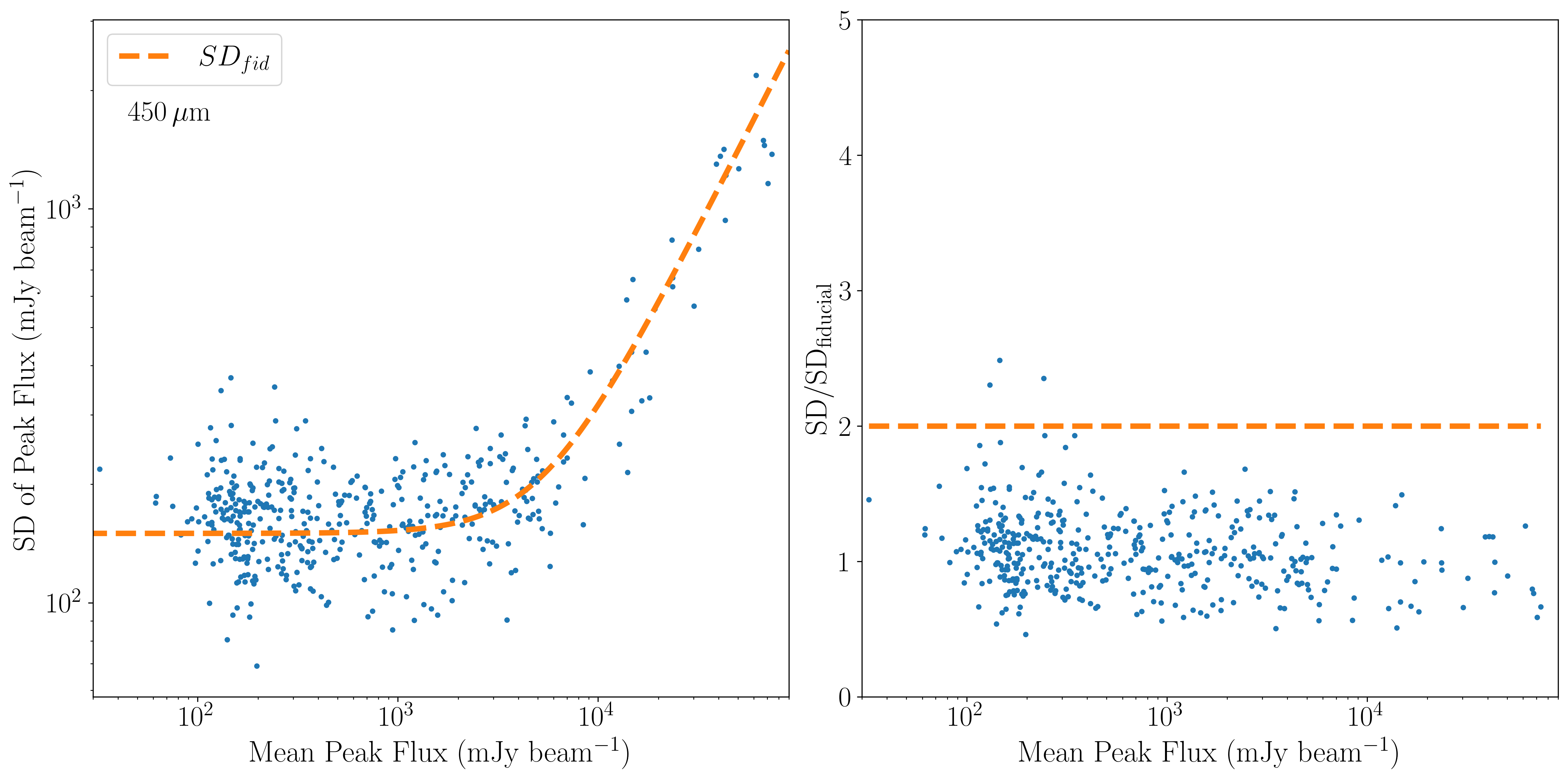
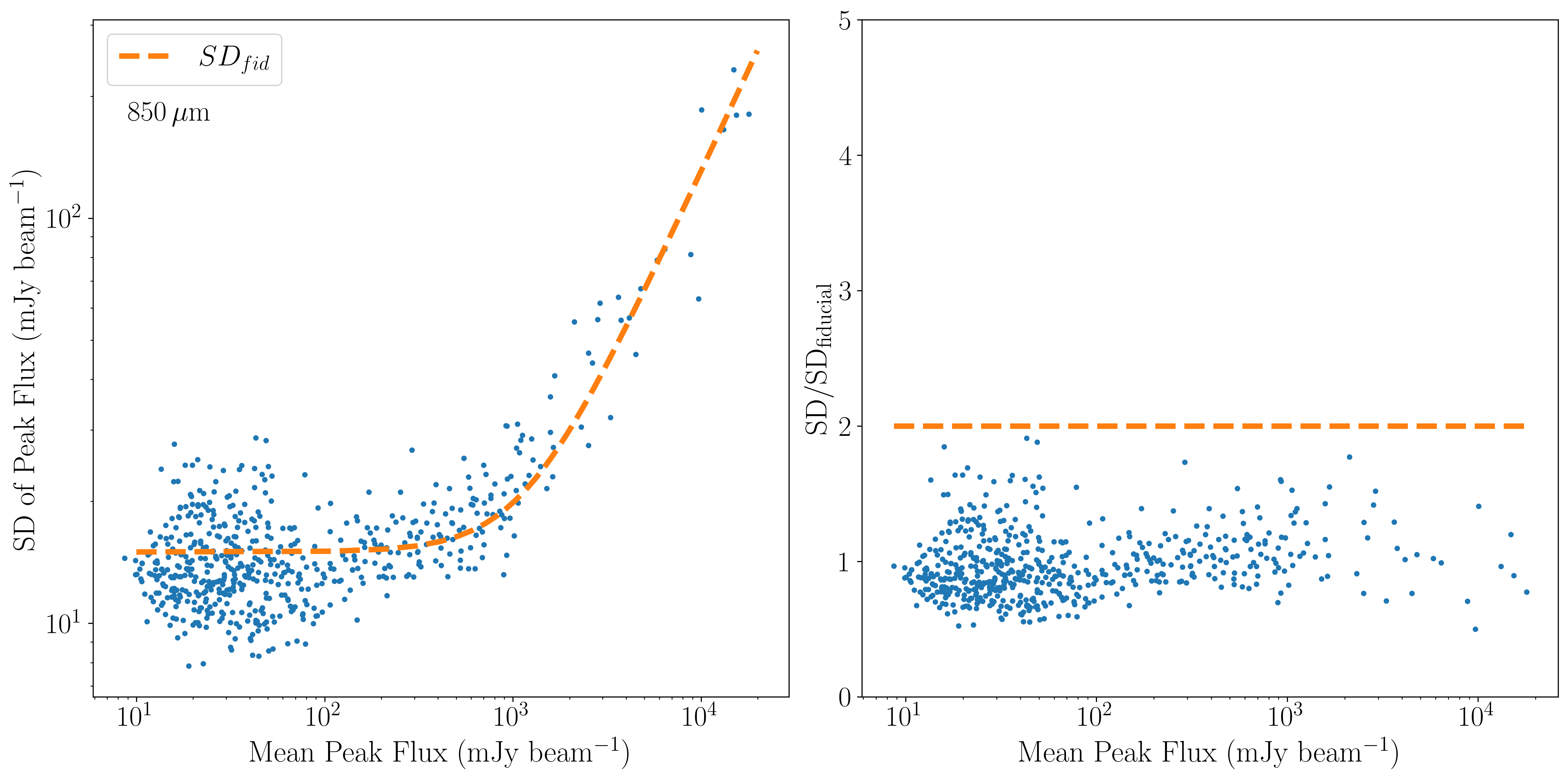
Figure 3: Left panels: Scatter plot of measured standard deviation of peak brightness versus measured mean peak brightness for all $450\,\mu$m (top row) and $850\,\mu$m sources (bottom row) in M 17. The orange dashed curve denotes the fiducial standard deviation, $\mathrm{SD_{fid}}$, for the expected uncertainty in the peak brightness of JCMT-SCUBA2 sources. Right panels: the same as the left panels, but for the normalized standard deviation of peak brightness ($SD/\mathrm{SD_{fid}}$). Here the dashed orange line separates out the potential stochastic variables.

2.2 Mid-IR Data Sets

2.2.1 Infrared-bright YSOs in M 17

M 17 is one of the most intensively studied massive star-forming regions in the Galaxy. Using data from several infrared studies, we collected a sample of YSOs that are located within the inner $40\arcmin$ diameter area of the JCMT field. The YSOs in the sample are identified via infrared excess from 2MASS and Spitzer observations (Povich et al., 2009; Povich & Whitney, 2010; Povich et al., 2013), with most of the sources being part of the Spitzer/IRAC candidate YSO catalog for the inner galactic midplane (SPICY; Kuhn et al., 2021). We also include a few massive YSOs classified from SOFIA/FORCAST observations for M17 at $19$ and $37\,\mu$m by Lim et al. (2020), and an outburst MYSO M 17 MIR by Chen et al. (2021).

Based on the above studies, we compile a catalog of 166 YSOs. These YSOs are predominantly in early evolutionary stages, with 34.9% Class I objects and 42.8% Class II objects. Class III YSOs are only a minor fraction (1.2%) of the sample, likely due to the complexity of identifying them in distant massive star-forming regions. A substantial fraction (21.1%) of the sample is assigned as ‘uncertain’ objects, whose infrared excess emission can also be explained by the circumstellar envelope surrounding the evolved post-main-sequence stars (Chen et al., 2013).

2.2.2 Multi-epoch WISE/NEOWISE Data

The Wide-field Infrared Survey Explorer (WISE, Wright et al. 2010) is a 40 cm telescope in a low Earth orbit that surveyed the entire sky in 2010 at 3.4, 4.6, 12, and $22\,\mu$m. The angular resolutions in the four bands (W1, W2, W3, and W4) are $6\farcs 1$, $6\farcs 4$, $6\farcs 5$, and $12\farcs 0$, respectively. The WISE telescope was reactivated as the Near-Earth Object WISE (NEOWISE Mainzer et al., 2011, 2014) program, which used only the short wavelength W1 and W2 bands to search for near-Earth objects. NEOWISE observations of M17 were obtained every 6 months from December 2013 until December 2022. Each visit consists of $10-20$ exposures taken over a few days.

For each source in the YSO sample, we first queried the WISE and NEOWISE single exposure catalogs (Wright et al., 2019; WISE Team, 2020) from the NASA/IPAC Infrared Science Archive (IRSA), using a radius $3\arcsec$, the same method used for the previous studies (Contreras Peña et al., 2020; Park et al., 2021, 2024). The average values of the Right Ascension (R.A.) and Declination (Decl.) in J2000 epoch are determined from all source positions of the same entry. We then selected single-exposure sources that are located within $2\times sd_{d}$ of this mean location (where $sd_{d}$ is the standard deviation of the distances from the mean location). The next step was to group all the single-exposure measurements performed within a few days of each other. Because we looked for long-trend mid-IR variability over years, we discarded the brightest and faintest 15% for each group. Using the remaining 70% of the group, we estimate the mean modified Julian date (MJD), the mean magnitude in W1 / W2, the mean error and the standard deviation (in magnitude) for each YSO matched in the specific epoch. The measurement error was then calculated by adding, in quadrature, the mean error and standard deviation in each epoch. This method then provides multi-epoch WISE/NEOWISE observations every 6 months. Finally, the WISE/NEOWISE surveys provide up to 19 epochs of W1 and W2 photometry for YSOs in M 17 in the period from 2010 to 2022. In particular, the multi-epoch W2 magnitudes of one YSO in M 17, which is not included by NEOWISE single exposure catalogs, was adopted from our previous paper (M17 MIR; Chen et al., 2021).

To obtain reliable results, we select YSOs with a minimum of 12 epochs in both W1 and W2 and a mean uncertainty $\mathrm{\sigma(mag)}<0.2$ mag. Only 66 of the 166 IR-bright YSOs compiled in §2.2.1 meet this requirement. The low number of reliable sources could be explained in part by the lower spatial resolution of WISE data as compared with Spitzer data, which is used to detect YSOs in our sample (see Section 2.2.2). In addition, the strong mid-IR emission from the photodissociation region (PDR) excited by the massive stars in M 17 worsens the sensitivity of the WISE single-exposure maps.

2.3 Far-IR and millimeter Data Sets

In order to characterize the far-IR emission from sources, we incorporated publicly available imaging observations from the Herschel Space Observatory (Herschel) and its PACS instrument at 70, 100, and 160 $\mu$m (Poglitsch et al., 2010). The Herschel data used in this work are Level 3.0 products of the PACS calibration observations towards M 17 (eight observations with IDs from 1342192767 to 1342192774), provided by the Herschel Science Archive. The pixel scales are $1\farcs 6$, $1\farcs 6$, and $3\farcs 2$ at 70, 100, and 160 $\mu$m, and the measured resolutions are $8\farcs 0$, $8\farcs 0$, and $12\farcs 0$, respectively.

We also include observations by the Atacama Compact Array (ACA) for M 17, obtained on 2019 April 17 (project ID 2018.1.01091.S, PI: M. Reiter) with 11 antennas of 7 m diameter in a fixed configuration. The projected baselines ranged from $\sim 8$ to 48 m. M 17 was observed in Band 6 (230 GHz, 1.3 mm) with six spectral windows (SPWs), three ($230.4735-230.5985$,$220.3335-220.4585$, and $219.4955-219.6205$ GHz) for the CO/¹³CO/C¹⁸O $J=2-1$ lines and three ($216.998-218.998$, $230.998-232.998$, and $230.9345-231.0595$ GHz) for continuum emission. The archival ACA Band 6 data were retrieved from the ALMA Science Archive at the National Radio Astronomy Observatory. Calibration and imaging were performed with CASA version 5.4 (McMullin et al., 2007), using the ALMA pipeline. Only the 1.3 mm continuum data is used in this study. The synthesized beam size of 1.3 mm continuum is $7\farcs 2\times 4\farcs 5$. The continuum sensitivity is $\sim 4.2\,\mathrm{mJy\,beam^{-1}}$.

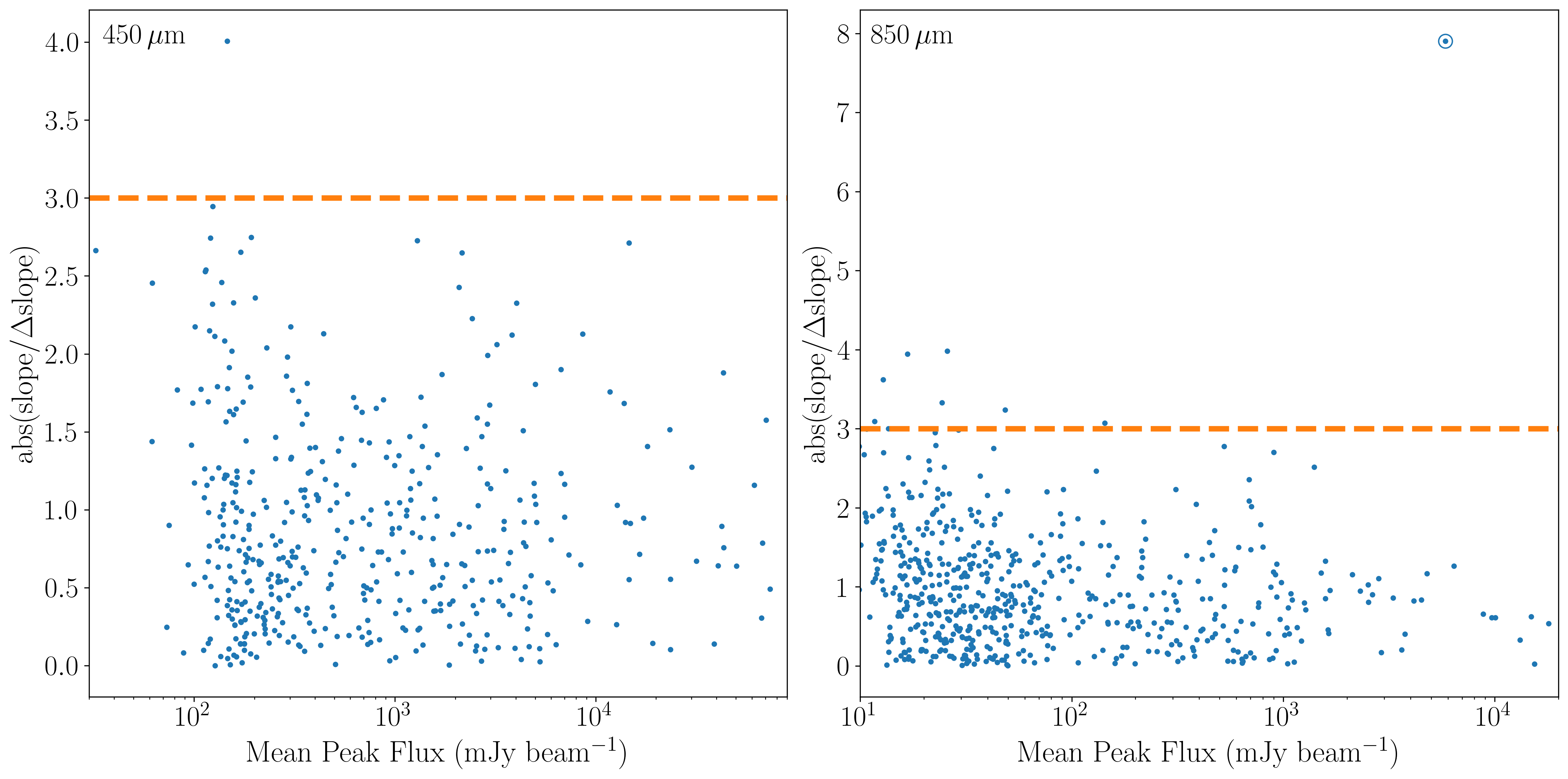
Figure 4: The distribution of the absolute value of the best-fit peak brightness slope $S$ ratioed to its uncertainty $\Delta S$ versus mean peak flux for the $450$ (left) and $850\,\mu$m (right) sources in M 17. The dashed horizontal line in both panels indicates where $|S/\Delta S|=3$, indicating the threshold for linear variability reliability as defined by Johnstone et al. (2018). Bright $450$ and $850\,\mu$m sources with $|S/\Delta S|>3$ are highlighted by circles. In the $850\,\mu$m plot, only one bright source JCMTPP J182023.2 has a value of $|S/\Delta S|$ much higher than the threshold.

3 Submillimeter and mid-IR variables

3.1 Searching for Submillimeter variables in M 17

Submillimeter variability of a given object can be categorized into three types: stochastic, secular, and single-epoch. The stochastic and secular variables can be selected via statistical investigations. We follow the methods outlined by Johnstone et al. (2018) to search for stochastic and secular variables. For each source, we extract the mean peak brightness in the co-added images and the brightness at the same location in each individual epoch. The standard deviation, $\mathrm{SD}$, in peak brightness across all epochs is then calculated for each source and shown in Figure 3.

The uncertainty in peak brightness for faint sources is dominated by the relatively uniform rms noise per epoch, while for bright sources the uncertainty in the relative calibration of the map will dominate. Johnstone et al. (2018) proposed a fiducial standard deviation $\mathrm{SD_{fid}}$ for the statistical investigation of the JCMT Transient survey, as

$$SD_{fid}(i)=\sqrt{(n_{\mathrm{RMS}})^{2}+(\sigma_{\mathrm{FCF}}\times f_{m}(i))^{2}}\,\mathrm{mJy\,beam^{-1}},$$ (1)

where $n_{\mathrm{RMS}}$ is the typical rms noise measured across the observed epochs (dominating faint sources), $\sigma_{\mathrm{FCF}}$ is the expected relative flux calibration uncertainty (dominating bright sources), and $f_{m}(i)$ is the mean peak flux of source $i$. For the 17 good epochs at $450\,\mu$m, we calculate $n_{\mathrm{RMS}}\approx 150\,\mathrm{mJy\,beam^{-1}}$ and $\sigma_{\mathrm{FCF}}\approx 2.8\%$, not far off the ensemble values, $130\,\mathrm{mJy\,beam^{-1}}$ and $3.5-5\%$, derived for the eight Gould Belt regions recalibrated with Pipeline V2 (Mairs et al., 2024). At $850\,\mu$m, the values of $n_{\mathrm{RMS}}\approx 15\,\mathrm{mJy\,beam^{-1}}$ and $\sigma_{\mathrm{FCF}}\approx 1.3\%$ are very close to the values of $15\,\mathrm{mJy\,beam^{-1}}$ and $1.5\%$ found for M17 SWex at $850\,\mu$m by Park et al. (2024).

The fiducial models for the 450 and $850\,\mu$m sources in M 17 are plotted as the orange dashed curves in the left column of Figure 3. The majority of $450$ and $850\,\mu$m sources lie near the fiducial models at each wavelength. To show this result more clearly, the right panels in Figure 3 plot the $\mathrm{SD}$ in units of the fiducial models (normalized $\mathrm{SD}$) as a function of mean source brightness at $450$ and $850\,\mu$m. Sources with a normalized $\mathrm{SD}$ that is clearly higher than unity are potential candidates for submillimeter variables. For example, the normalized $\mathrm{SD}$ of EC 53 (V371 Ser) was found to be as high as 5.6 at $850\,\mu$m (Johnstone et al., 2018) and clear a strong submillimeter variable (Yoo et al., 2017; Lee et al., 2020; Francis et al., 2022).

As shown in Figure 3, we find no $450\,\mu$m sources brighter than $0.65\,\mathrm{Jy\,beam^{-1}}$ showing a normalized $\mathrm{SD}$ of peak brightness greater than 2. Also, we find no $850\,\mu$m sources with a normalized $\mathrm{SD}$ of peak brightness greater than 2. From analyses of the standard deviation of the source peak brightness at $450$ and $850\,\mu$m, we find that the submillimeter sources in M17 do not have observable stochastic variability over few year timescales.

We next consider secular peak brightness change over time. We determine the peak brightness slope (fractional change per yr) using a statistical analysis, the same approach undertaken for the eight Gould Belt regions by Johnstone et al. (2018). For each source $i$, we derive a model fit, $f_{l}(i,t)$, that is linear over time, $t$, with two derived parameters: initial flux, $f_{0}(i)$ at time $t_{0}$, the time of the first epoch, and slope, $S(i)$, measured in fractional brightness change per year:

$$f_{l}(i,t)=f_{0}(i)\left(1+S(i)(t-t_{0})\right).$$ (2)

Furthermore, in order to measure the relevance of any slopes departing from flat ($S=0$; there are no changes in brightness over time) we also compute the uncertainty of the slope, $\Delta S$. In Figure 4, the distribution of the absolute value of the best-fit slope in units of $\Delta S$ versus mean peak brightness is shown for the $450$ and $850\,\mu$m sources in the left and right panels, respectively. We find that none of the $450\,\mu$m sources brighter than $0.65\,\mathrm{Jy\,beam^{-1}}$ have $|S|/\Delta S$ greater than 3, a reasonable threshold for the detection of robust linear submillimeter variables (e.g. Johnstone et al., 2018).

A bright $850\,\mu$m source, JCMTPP J182023.2, with an $|S|/\Delta S=7.8$ stands out as a linear variable in the right panel of Figure 4, with a total linear increase of $\sim 4-5\%$ over 3.5 years. The $850\,\mu$m lightcurve of JCMTPP J182023.2 is shown in Figure 5. JCMTPP J182023.2 is a bright and compact continuum source observable from submillimeter to millimeter wavelengths and associated with a 22-GHz H₂O maser (Hobson et al., 1993; Hill et al., 2005; Di Francesco et al., 2008; Breen & Ellingsen, 2011). The $450\,\mu$m counterpart of JCMTPP J182023.2 has $|S|/\Delta S=1.27$. Given the relatively high flux calibration uncertainty at $450\,\mu$m of $\sim 3$% derived earlier, an observed fractional change of $\sim 1$%/yr would not be recovered before many years of observation.

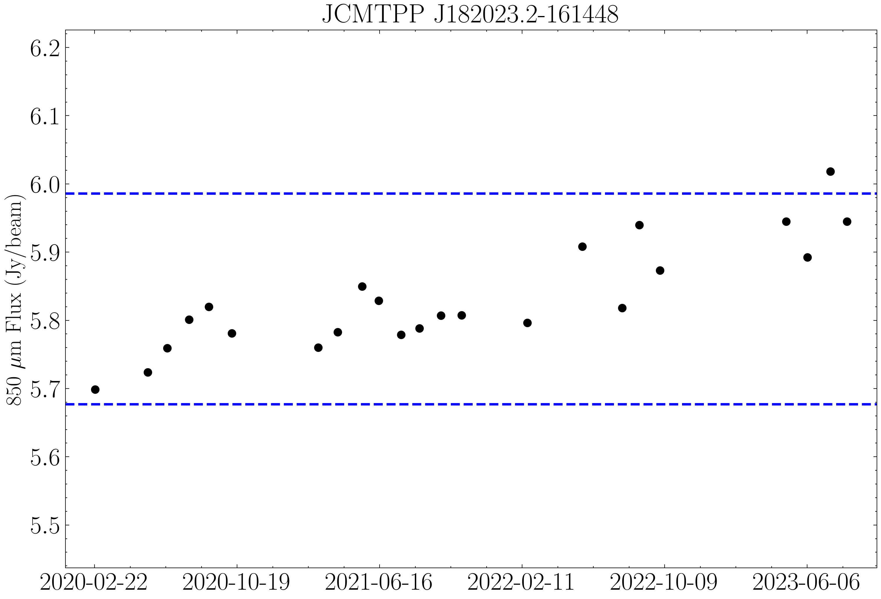
Figure 5: $850\,\mu$m light curve of the candidate linear variable JCMTPP_J182023.2. The blue dashed lines represent the upper and lower boundaries of $\pm 2SD_{\mathrm{{fid}}}$, where $SD_{\mathrm{{fid}}}$ is the expected fiducial standard deviation.

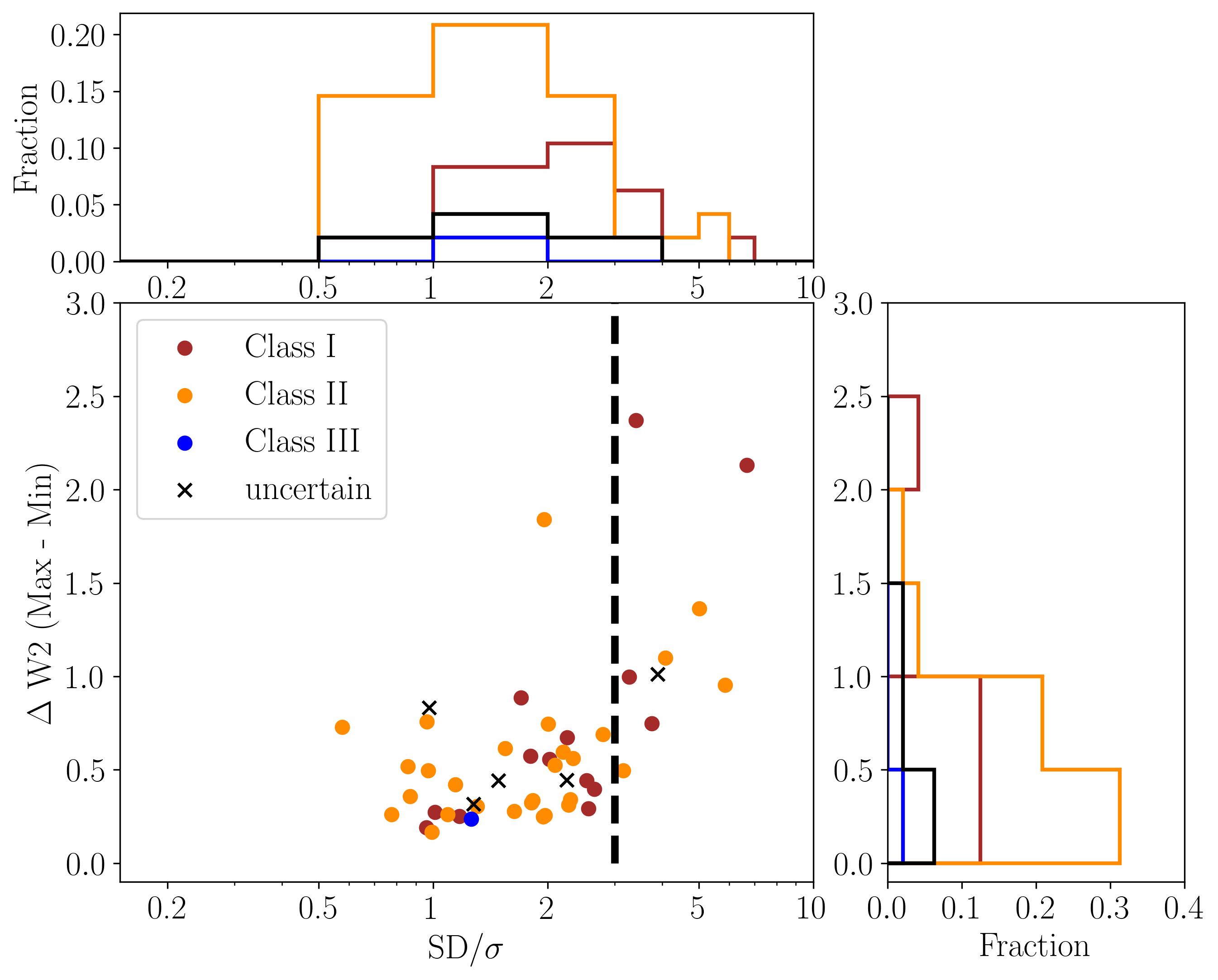
Figure 6: The distribution of the $\Delta W2$ versus $SD/\sigma$ for the YSO sample with $\Delta\mathrm{W2}/\sigma\mathrm{(W2)}>3$. The vertical dashed line indicates the commonly used threshold value of $SD/\sigma=3$ for identifying variable sources.

3.2 Searching for variable YSOs in the mid-IR

We uncovered a sample of 66 YSOs in M 17 with reliable multi-epoch data in the WISE W1 and/or W2 bands. Some of the deeply embedded YSOs, for example M17 MIR (Chen et al., 2021), are very faint or not detected at all in the W1 band. Therefore, and following Park et al. (2021), the mid-IR light curve analysis for the majority of the sample is based on the multi-epoch data in the W2 band, supplemented with analysis of W1 data for specific sources.

For the 66 YSOs with at least 12 epochs of photometry, we obtained their variability amplitude of W2 magnitude $\Delta\mathrm{W2}$, the difference between the maximum and minimum magnitudes, and their mean uncertainty of W2 magnitude $\sigma\mathrm{(W2)}$. Park et al. (2021) employed a criterion of $\Delta\mathrm{W2}/\sigma\mathrm{(W2)}>3$ to exclude sources that are unlikely to be variable and to search for variability in the sources remaining. After applying this criterion, they divided the mid-IR variability of YSOs in the Gould Belt into two major types, secular and stochastic variables. According to their mid-IR light curves, the secular variables can be further split into three categories, linear, periodic, and curved; while the stochastic variability includes burst, drop, and irregular (see definitions in Park et al., 2021).

We first examine YSOs with $\Delta\mathrm{W2}/\sigma\mathrm{(W2)}>3$ in the magnitude domain to find variability. Within the sample of 66 YSOs with NEOWISE data in at least 12 epochs, 48 sources satisfy this criterion. We applied the same methods as in Park et al. (2021), to these 48 YSOs to investigate their types of variability.

We estimate a flux standard deviation ($\mathrm{SD}$) and a mean flux uncertainty ($\sigma$) for the 48 YSOs with $\Delta\mathrm{W2}/\sigma\mathrm{(W2)}>3$. Figure 6 the distribution of these YSOs in the diagram of $\Delta\mathrm{W2}$ versus $\mathrm{SD}/\sigma$. Similarly as Park et al. (2021), we employed the criterion of $\mathrm{SD}/\sigma>3$ to classify variables in general. Nine YSOs have $\mathrm{SD}/\sigma>3$, and are all at younger stages (Class I, II), with the exception for one source (SPICY 82001) which has an uncertain classification.

Some YSOs in Figure 6 show large brightness variations despite having $\mathrm{SD}/\sigma$ values less than 3. Previously, Park et al. (2021) found that some types of YSO variability may not lead to a large $\mathrm{SD}$ over the full light curve. In order to classify as many variables as possible, we also applied the Lomb-Scargle periodogram (LSP) (Lomb, 1976; Scargle, 1989) to the mid-IR light curves using the LombScargle from python package astropy. Since the WISE/NEOWISE surveys have a 6 month cadence, periodic variations with periods shorter than 6 months cannot be extracted from the data. Furthermore, light curves with periods longer than 2300 days cover fewer than two full phases, since the total duration of the NEOWISE data is about 4600 days (12.5 years). Given this, we cannot conclude that these are variable YSOs with long periodic (periods longer than 2300 days) variability. Periods longer than 2300 days manifest as an increasing or decreasing trend in mid-IR brightness. To quantify the significance of the amplitude and period, we compute the false alarm probability (FAP) of LSP analysis, $\mathrm{FAP_{LSP}}$. This provides the uncertainty of a particular LSP peak by quantifying the probability of a false peak due to random errors. We slightly modified the method by Baluev (2008) to determine the FAP of the found period or longer, rather than summing over all periods within the range checked (see also Park et al., 2021; Lee et al., 2021).

We further adopted a linear least-squares fit to find a linear trend of increasing or decreasing fluxes. Light curves with good linear fits are also often fitted by LSP with a very long period. We define the linear FAP (hereafter $\mathrm{FAP_{Lin}}$, with the same method as Lee et al. (2021), to estimate the likelihood of the determined best-fit linear slope. If the value of $\mathrm{FAP_{Lin}}$ of a given source is $<10^{-4}$, the light curve of this source can be robustly fitted by a linear slope. For LSP analysis, a somewhat lower threshold, $\mathrm{FAP_{LSP}}<10^{-2}$, is used to explore the wide range of periods and amplitudes recovered. This lower threshold results in a few false positives within the LSP sample; however, we have checked to ensure that these false positives result only in a small contamination fraction.

In Figure 7, we consider both the periodic and linear FAPs for the best fits to the 48 YSOs with $\Delta\mathrm{W2}/\sigma\mathrm{(W2)}>3$. Sources with $\mathrm{FAP_{Lin}}\leqslant 10^{-4}$ lying in the upper region in Figure 7 are classified as showing linear variability. For the remaining sources with $\mathrm{FAP_{LSP}}\leqslant 10^{-2}$, those with a period of 2300 days or less are classified as periodic variables, and those with a longer period are classified as showing curved variability. Finally, 14 out of the initial 48 candidate variables are classified as curved (6), periodic (6) and linear (2). In general, we categorize them as secular variables.

The candidate variable sources that fail the conditions of secular variability are classified as stochastic. An additional constraint is applied to identify sources that exhibit bursts or drops in brightness at some epochs while maintaining stable fluxes over the remaining epochs. Sources with median(W2) - min(W2) $>0.8\times\Delta\mathrm{W2(max-min)}$ are burst type, and those with max(W2) - median(W2) $>0.8\times\Delta\mathrm{W2(max-min)}$ are drop type. After excluding all previously identified sources, those with $\mathrm{SD}/\sigma>3$ are classified as irregular variables. In particular, we reclassify the outbursting MYSO M17 MIR as irregular due to a high value of $\mathrm{SD}/\sigma=6.69$, despite the roughly linear trend ($\mathrm{FAP_{Lin}}=8.28e-06$) of its mid-IR light curve (see also Figure 12).

Following the taxonomy of mid-IR variability (Park et al., 2021), we classify the variability types for 22 out of the 48 YSOs with $\Delta\mathrm{W2}/\sigma\mathrm{(W2)}>3$. The remaining 26 YSOs cannot pass any criterion for secular and stochastic variables. Table 2 summarizes the statistical results of the types of variability along with the evolutionary stages for the 22 YSOs with mid-IR variability. For completeness, the statistics of all 22 variable YSOs are presented in Table 6. Two YSOs (#6 and #10 in Table 6) show more pronounced variability in W1 than in W2, so their variability types are classified from the W1 band.

Fourteen of the 22 variable YSOs in M 17 identified in this study are secular variables, while the remaining 8 stochastic variables are dominated by irregular types. Almost all (19) of the 22 variables are Class I and II YSOs, only three variable YSOs are of uncertain stage. Although the number of Class I variables is smaller than that of Class II variables, the fraction (38.1%) of Class I YSOs with mid-IR variability is higher than that (29.7%) of the Class II YSO sample.

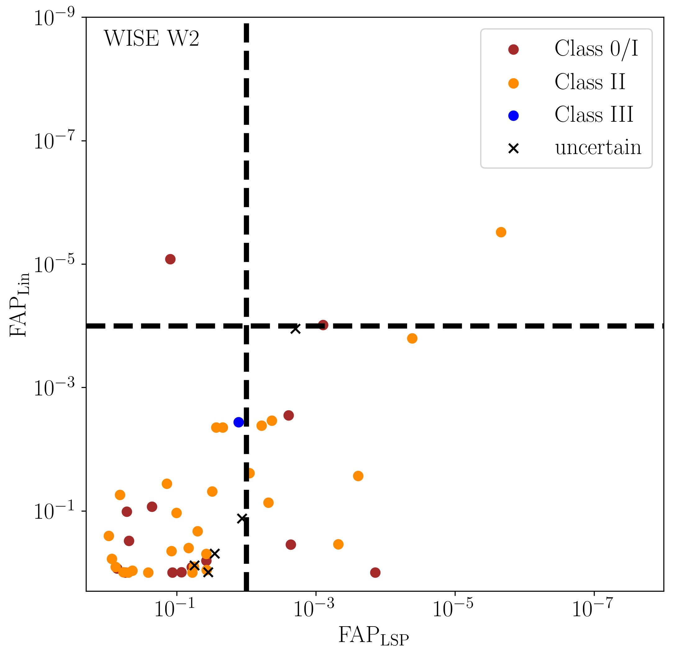
Figure 7: Comparison of the FAPs for linear and periodic fits for the same YSO as in Figure 6. The vertical dashed line represents a FAP value of $10^{-4}$ for linear fit, while the horizontal dashed line represents a FAP value of $10^{-2}$ for LSP fit.

Table 2: MIR Variability Type by YSO Classification

Variability type	Class I	Class II	Class III	uncertain	Total
Linear	1 (4.8)	1 (2.7)	0	0	2
Curved	2 (9.5)	3 (8.1)	0	1 (14.3)	6
Periodic	2 (9.5)	3 (8.1)	0	1 (14.3)	6
Burst	1 (4.8)	2 (5.4)	0	0	3
Drop	0	0	0	0	0
Irregular	2 (9.5)	2 (5.4)	0	1 (14.3)	5
Total	8 (38.1)	11 (29.7)	0	3 (42.9)	22
All YSOs	21	37	1	8	66

Note. — Numbers are the count of variables for each variable type, while numbers in parentheses are the fraction (%) of variable candidates relative to the selected samples in each evolutionary stage .

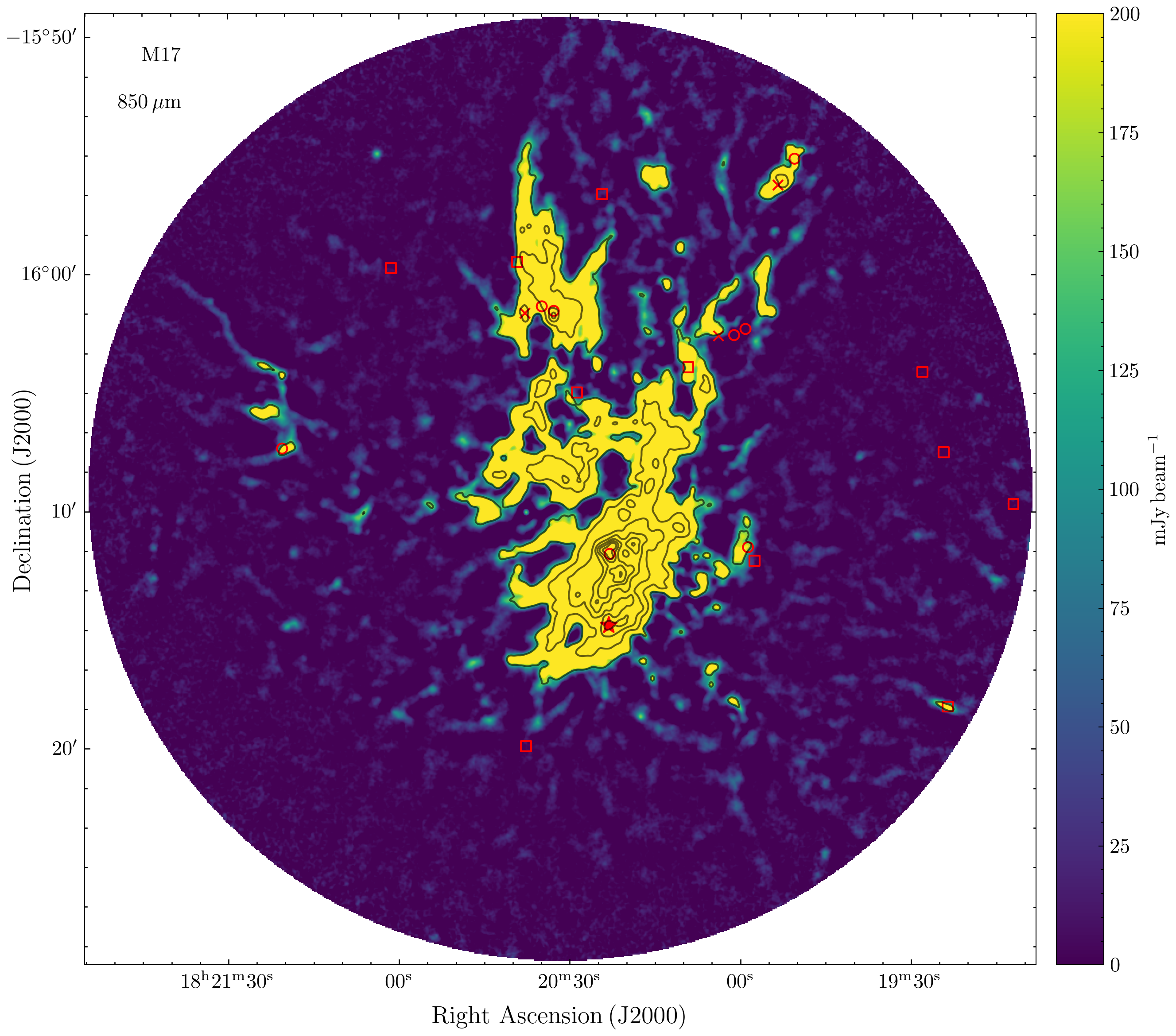
Figure 8: The spatial distribution of mid-IR and submillimeter variable candidates classified in this work, overlaid on the $850\,\mu$m map of M 17. The contours of $850\,\mu$m continuum emission are in levels of 0.15, 0.6, 1.8, 3.6, 6.0, 9.0, 1.26 and $1.68\,\mathrm{Jy\,beam^{-1}}$. Figure 2. Circle, square, and ‘X’ represent different classification type for YSOs, i.e., Class I, Class II, and uncertain, respectively. The star symbol represents the linear variable at $850\,\mu$m (JCMTPP_J182023.2).

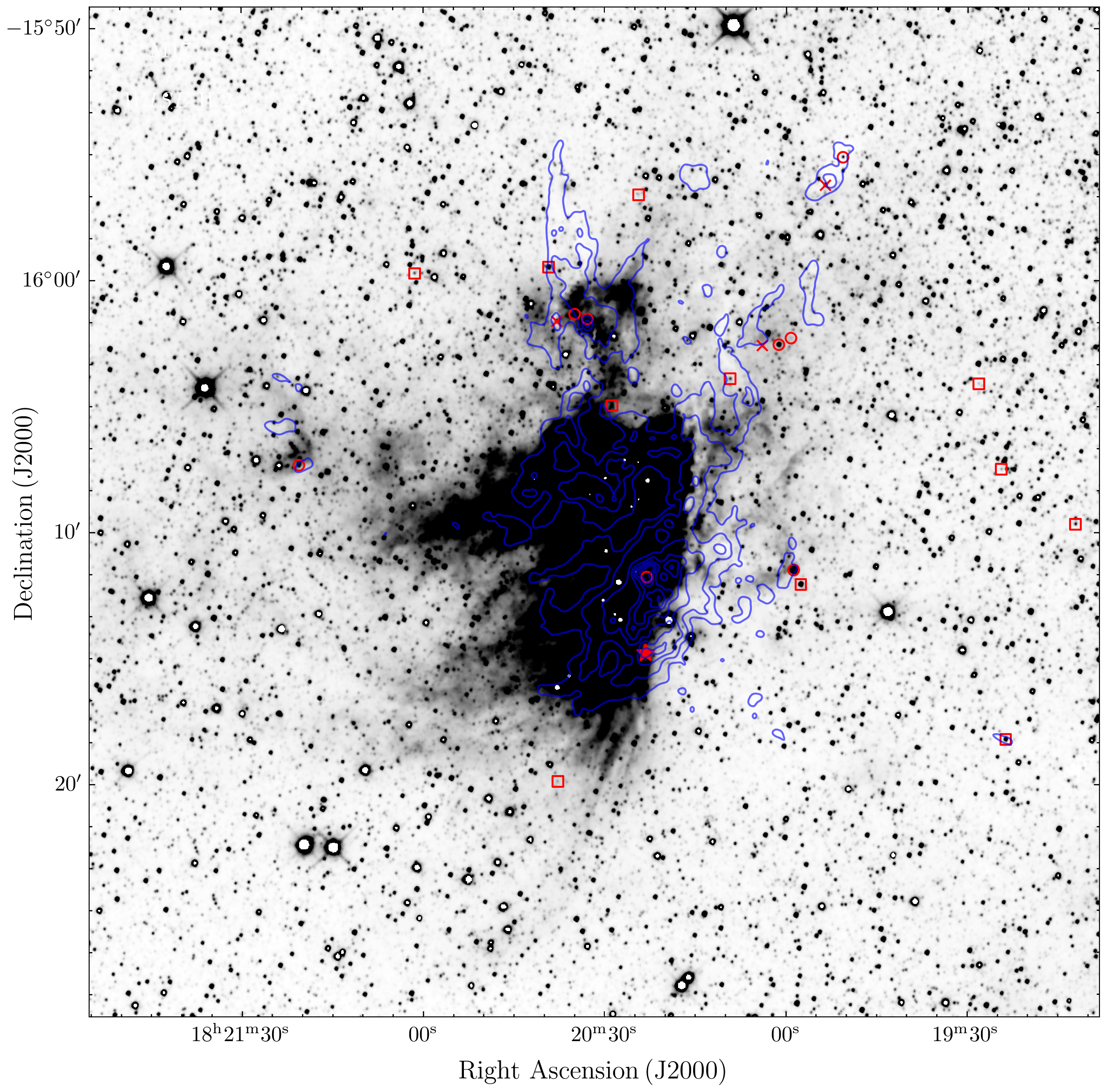
Figure 9: Same as Fig. 8, but for the mid-IR WISE W2 map in gray scale. The contours of $850\,\mu$m continuum emission are as same as in Figure 8 but are displayed as blue.

3.3 Cross-matching the submillimeter sources with the variable YSOs

For the 22 YSOs showing mid-IR variability, we searched for the nearest submillimeter sources at 450 and $850\,\mu$m. Four variable YSOs have bright counterparts at $450\,\mu$m and six variable YSOs have bright counterparts at $850\,\mu$m within a radius of $10\arcsec$ (Table 3), following the distance constraint applied by Contreras Peña et al. 2020. We manually checked the spatial distribution of the 22 variable YSOs overlaid on the 450 and $850\,\mu$m maps. Expanding the search radius to $15\arcsec$ leads to one additional potential submillimeter counterpart for SPICY 81957.

Among the seven variable candidate YSOs with submillimeter counterparts, four YSOs (SPICY 81351, 82315, 81642, and 81623) are located on the outskirts of the M 17 region. Two of these candidate YSOs, SPICY 81642 and 81623, have periods of 437.8 and $>4800$ days, respectively. Both have an uncertain class for their YSO classification (Povich et al., 2013; Kuhn et al., 2021). We suggest SPICY 81642 and 81623 are likely contamination from evolved post-main-sequence stars with periods typically longer than hundreds of days (e.g., Yin et al., 2021). The remaining two variables (SPICY 81351 and 82315) have an irregular variability type and are closer to their nearby submillimeter peaks than the former two. We suggest that SPICY 81351 and 82315, as well as their submillimeter counterparts, are parts of the M 17 complex, but spatially distinct from the M 17 H II region. The remaining three variable YSO candidates, SPICY 81957 and 82001, and M17 MIR, are located at the two star-forming clouds M17 North and SW, respectively. We will discuss them in more detail in Sect. 4.1.

Table 3: Matched variable YSO candidates and $450$ or $850\,\mu$m sources within a radius of $15\arcsec$.

#	Variable YSO	$450\,\mu$m source	Separation ($\arcsec$)	$850\,\mu$m source	Separation ($\arcsec$)
2	SPICY 81351	JCMTPP_J181923.8	3.1	JCMTPP_J181923.4	5.2
5	SPICY 81623	-	-	JCMTPP_J181950.6	7.0
6	SPICY 81642	JCMTPP_J181954.0	12.0	JCMTPP_J181953.9	8.4
15	SPICY 81957	JCMTPP_J182032.9	15.0	JCMTPP_J182032.8	12.0
18	SPICY 82001	JCMTPP_J182038.1	6.2	JCMTPP_J182038.2	5.6
21	SPICY 82315	JCMTPP_J182120.2	6.4	JCMTPP_J182120.1	6.9
22	M17 MIR	JCMTPP_J182022.7	9.2	JCMTPP_J182022.8	7.0

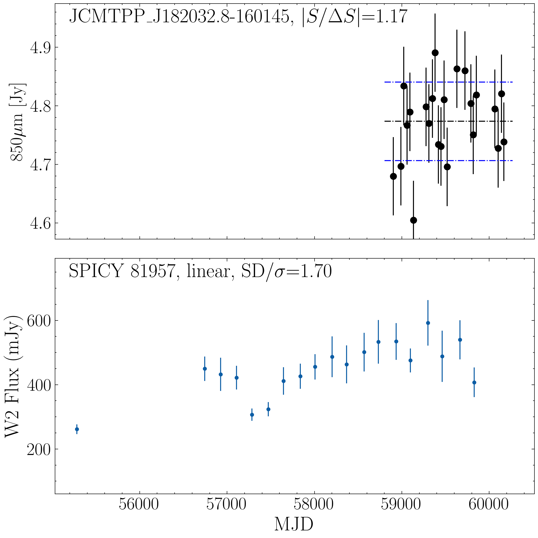
Figure 10: JCMT Transient $850\,\mu$m (top) and NEOWISE W2 light curves (bottom) of SPICY 81957. The black and blue dashed lines in the JCMT Transient light curve represent the mean peak flux and $\pm 1\sigma$ boundaries.

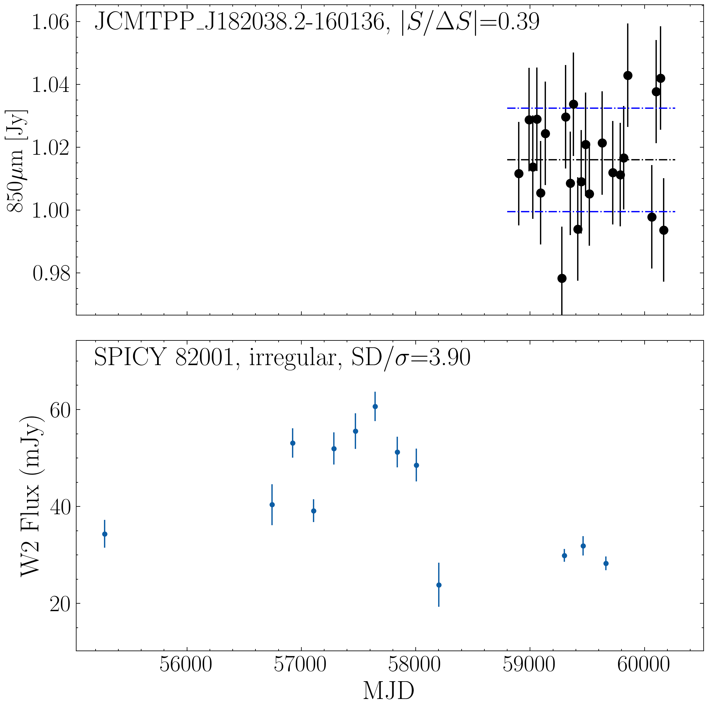
Figure 11: Same as Figure 10 but for SPICY 82001.

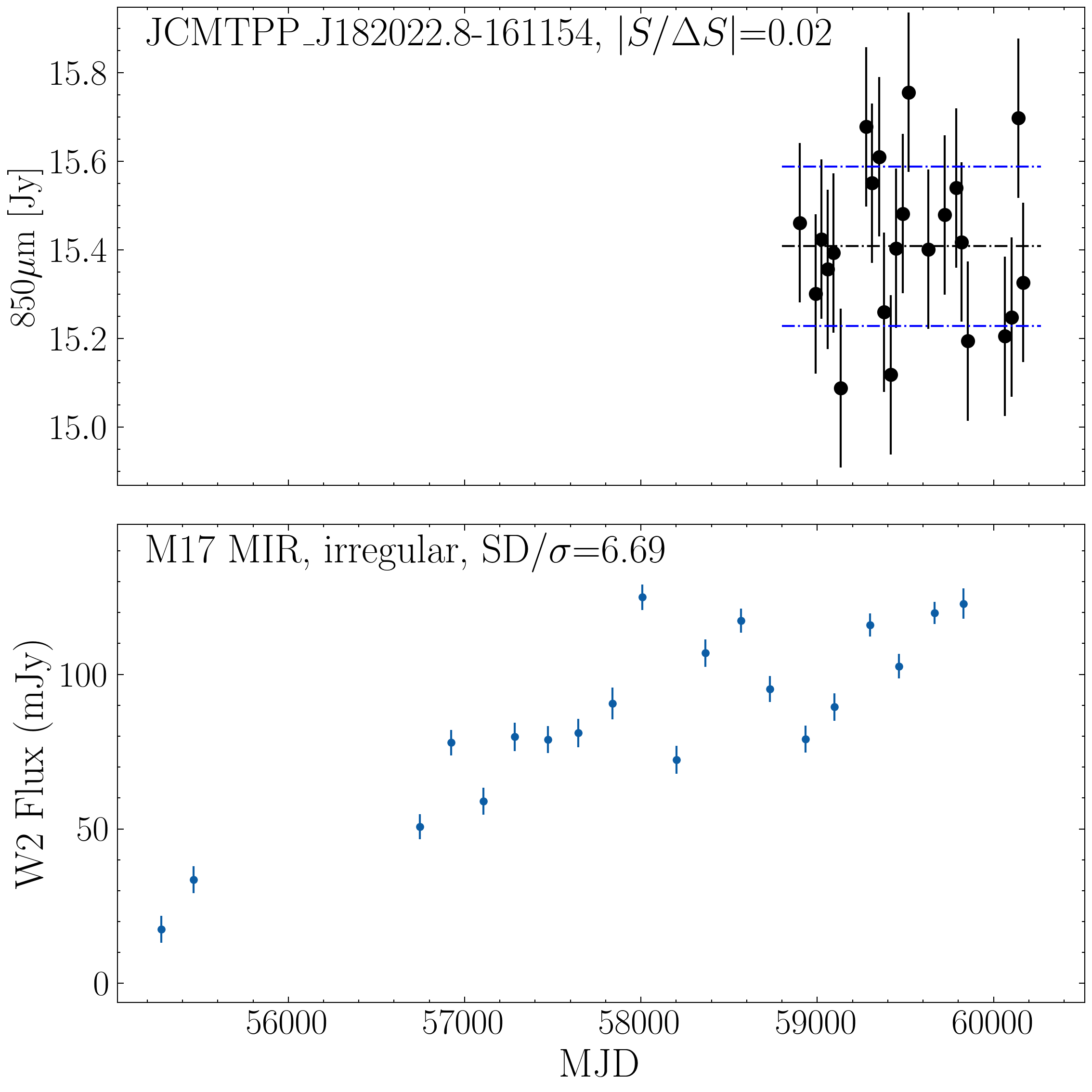
Figure 12: Same as Figure 10 but for M17 MIR.

Figure 13: Multiwavelength maps for JCMTPP_J182023.2, collected from Herschel (70, 100, and $160\,\mu$m), JCMT Transient Survey (450 and $850\,\mu$m), and 1.3 mm continuum by ACA. The red cross denotes the position of 22 GHz H₂O maser source (Breen & Ellingsen, 2011).

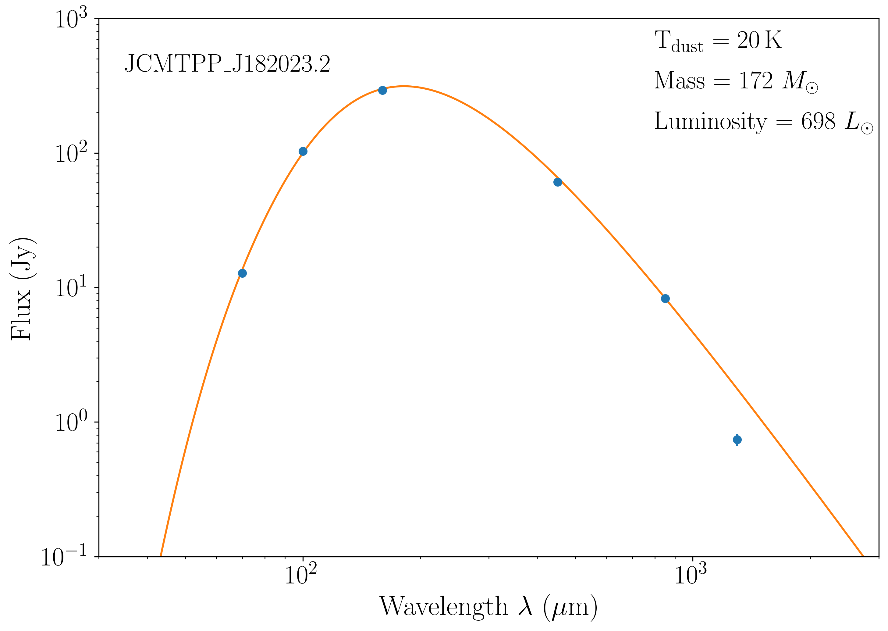
Figure 14: Spectral energy distribution of the linear variable JCMTPP_J182023.2. The best-fit greybody model is shown as the orange curve.

4 Discussion

4.1 Interesting YSOs with mid-IR variability

SPICY 81957 is located at the boundary of a bright JCMT source seen at 450 and $850\,\mu$m, the strongest submillimeter peak in M17 North, labeled as M17N by Reid & Wilson (2006). H₂O maser emission at 22.2 GHz was detected towards this submillimeter source (Jaffe et al., 1981). SPICY 81957 is the brightest variable YSO in the mid-IR found in this study, modeled as a candidate MYSO of $5-10\,M_{\sun}$ (Povich et al., 2009). The JCMT Transient $850\,\mu$m and WISE/NEOWISE W2 light curves of SPICY 81957 are presented in Figure 10. SPICY 81957 shows significant mid-IR variability over $\gtrsim 10$ years period. Its submillimeter light curve provided by JCMT Transient Survey covers only the recent $\sim 3.5$ years, a small fraction of the NEOWISE timescale. The mid-IR flux of SPICY 81957 is roughly stable throughout most of the period of JCMT Transient survey, except for 2022 September when the W2 flux decreased by a factor of $\sim 50\%$ compared to that in 2022 March. However, the presumably linear decrease of $850\,\mu$m peak flux of the associated submillimeter source (JCMTPP_J182032.8) between 2022 September and 2023 August cannot be confirmed from the JCMT Transient survey data collected in 3.5 years.

SPICY 82001 is associated with the second brightest submillimeter peak in M17 North. The evolutionary class of SPICY 82001 is still in debate; Povich et al. (2013) classified it as a Class II/III YSO, while the SPICY catalog assigned an ambiguous type (Kuhn et al., 2021). Figure 11 shows the $850\,\mu$m and WISE/NEOWISE W2 light curves for this source. SPICY 82001 has been at its faintest mid-IR phase over the period of JCMT Transient survey. The $850\,\mu$m light curve of the associated submillimeter source JCMTPP_J182038.2 is also flat, in line with expectation.

M17 MIR is associated with the second brightest JCMT source at 450 (JCMTPP_J182022.7) and $850\,\mu$m (JCMTPP_J182022.8) throughout the M 17 field. M17 MIR is located at the M17 SW cloud, adjacent to the M 17 H II region. Chen et al. (2021) found that M17 MIR has produced two accretion outbursts in recent decades, one major accretion outburst in the 1990s and one ongoing moderate accretion outburst since mid-2010. Hobson et al. (1993) derived a total mass of $330\,M_{\sun}$ and a luminosity of $8000\,L_{\sun}$ for the natal clump of M17 MIR (FIR3 in their work) using multi-wavelength maps ranging from 450 to $1300\,\mu$m. The $850\,\mu$m and WISE/NEOWISE W2 light curves of M17 MIR are shown in Figure 12. M17 MIR shows significant mid-IR variability over $\gtrsim 10$ years period. During the JCMT Transient Survey period, the mid-IR variability of M17 MIR is mild, at a level of $\sim+50\%$. In contrast, the $850\,\mu$m light curve of M17 MIR suggests no submillimeter variability in the same period.

There are a number of potential reasons for the discrepancy between the mid-IR variability and the currently stable submillimeter peak flux of the three YSOs. First, based on the NEOWISE and JCMT Transient Survey for the Gould Belt, Contreras Peña et al. (2020) found that 39 YSOs are variable in at least one of the two surveys. However, only 14 of the 39 YSOs show correlated secular variability in mid-IR and submillimeter wavelengths. Second, given the farther distance compared to the Gould Belt, a single JCMT beamsize at $850\,\mu$m encompass more gas and dust for the protostars in M 17 than for those in the Gould Belt. This is likely to have an impact on the submillimeter variability and will be discussed below in Sect. 4.2 alongside the only secular submillimeter variable discovered in M 17 and in Sect. 4.4 compared to other fields of JCMT Transient Survey.

4.2 Candidate linear variable at $850\,\mu$m in M 17

JCMTPP_J182023.2 is the only candidate linear variable at $850\,\mu$m recovered by the JCMT Transient Survey for M 17. This source, however, is not visible in the mid-IR with either Spitzer or WISE. The protostar(s) embedded within JCMTPP_J182023.2 is therefore still infrared faint, and the soure is likely at an earliest stage.

Figure 13 presents continuum maps centered on JCMTPP_J182023.2 at far-IR through millimeter wavelengths, including Herschel 70, 100, $160\,\mu$m, JCMT-SCUBA2 450 and $850\,\mu$m, and ACA 1.3 mm. JCMTPP_J182023.2 starts to appear in the Herschel $70\,\mu$m image, although it remains still faint. Interestingly, the 22 GHz H₂O maser emission (Breen & Ellingsen, 2011), denoted by the red cross in all maps, spatially coincides with JCMTPP_J182023.2. Very young and embedded protostars are expected to power bipolar jets, which physically interact with ambient materials in their immediate environment (Zhou et al., 2024). In particular, 22.2 GHz H₂O maser emission emerges from the shocked molecular gas at the interface between the fast flow and the ambient material, thus efficiently tracing protostellar outflows (e.g., Furuya et al., 2005; De Buizer et al., 2005; Moscadelli et al., 2013). The 22.2 GHz H₂O maser emission associated with JCMTPP_J182023.2 suggests that this compact submillimeter source might host one or more deeply embedded protostar(s) that power protostellar powerful outflow(s). We also note a signature of molecular outflow for the CO ($2-1$) line emission around JCMTPP_J182023.2 from the ACA band 6 data. The integrated map of the CO ($2-1$) line wing emission clearly show a bipolar molecular outflow roughly perpendicular to the orientation of the elongated core seen in 1.3 mm dust continuum.

The integrated flux of JCMTPP_J182023.2 at multiple wavelengths is extracted using an aperture size equal to the beam size of each map. Figure 14 shows the spectral energy distribution (SED) of JCMTPP_J182023.2 constructed from the multiwavelength fluxes. We also obtain a best-fitting greybody dust temperature of $20\,\mathrm{K}$ from the SED fitting procedure ‘CMCIRSED’ developed by Casey (2012).

Assuming the submillimeter and millimeter emission is optically thin, the observed submillimeter and millimeter emission of JCMTPP_J182023.2 can be used to derive the mass of this source using

$$M=\frac{S^{\mathrm{int}}_{\lambda}\,d^{2}}{\kappa_{\lambda}\,B_{\lambda}(T_{\mathrm{d}})},$$ (3)

where $S^{\mathrm{int}}_{\lambda}$ is the integrated flux at wavelength $\lambda$, $d$ is the distance to M 17, $\kappa_{\lambda}$ is the dust opacity per unit mass at wavelength $\lambda$, and $B_{\lambda}(T_{\mathrm{d}})$ is the Planck function evaluated at the dust temperature $T_{\mathrm{d}})$. For this work, we choose $d=2.0\,\mathrm{kpc}$ (Xu et al., 2011), $\kappa_{850}=0.019\,\mathrm{cm^{2}\,g^{-1}}$ at $850\,\mu$m and $\kappa_{1.3}=0.013\,\mathrm{cm^{2}\,g^{-1}}$ at 1.3 mm (Lin et al., 2021), and $T_{\mathrm{d}}=20\,\mathrm{K}$. The values of $\kappa_{850}$ and $\kappa_{1.3}$ are converted to opacity relative to gas mass by assuming a standard gas-to-dust ratio of 100. The integrated flux of JCMTPP_J182023.2 is $8.3\,\mathrm{Jy}$ and $0.74\,\mathrm{Jy}$ at $850\,\mu$m and 1.3 mm, respectively. This source is also detected at 1.2-mm continuum emission with an FWHM of $43\arcsec$ by SIMBA observations with the Swedish ESO Submillimeter Telescope (Hill et al., 2005) and the authors report an integrated flux of 3.6 Jy and a peak flux of $1.6\,\mathrm{Jy\,beam^{-1}}$. Thus, we warn that the 1.3 mm ACA observations might recover only a small fraction of the total flux. The mass of JCMTPP_J182023.2 derived from its $850\,\mu$m integrated flux is $172\,M_{\sun}$, which characterizes the envelope. A slightly higher value ($\sim 190\,M_{\sun}$) for the envelope mass is obtained from the 1.2 mm SIMBA observations, where $\kappa_{1.2}=0.014\,\mathrm{cm^{2}\,g^{-1}}$ scaled from $\kappa\propto\lambda^{-1}$ and $\kappa_{1.3}=0.013\,\mathrm{cm^{2}\,g^{-1}}$ (Lin et al., 2021). Meanwhile the core mass of JCMTPP_J182023.2, traced by the compact source seen at the ACA 1.3 mm continuum emission, is $\sim 45\,M_{\sun}$, roughly a quarter of the envelope mass.

The bolometric luminosity of JCMTPP_J182023.2 is $698\,L_{\sun}$, calculated by integrating the best-fit greybody SED in the range from mid-IR to millimeter and assuming that the radiation from the central protostar is fully absorbed and then redistributed by dust through mid-IR to millimeter wavelengths. The envelope mass and bolometric luminosity locate JCMTPP_J182023.2 in the region for the accretion phase characterized by the roughly vertical evolutionary track in the luminosity versus mass diagram (Molinari et al., 2008). According to the classification of evolutionary stages in massive star formation (Urquhart et al., 2022), JCMTPP_J182023.2 is of the protostellar type. The luminosity-to-mass ($L_{\mathrm{bol}}/M_{\mathrm{env}}$) ratio of $4\,L_{\sun}\,M_{\sun}^{-1}$ for JCMTPP_J182023.2 is in line with the $L_{\mathrm{bol}}/M_{\mathrm{env}}$-ratio of $\sim 0.2-5\,L_{\sun}\,M_{\sun}^{-1}$ for the protostellar type and overlaps with the YSO type in the range $\sim 0.7-14\,L_{\sun}\,M_{\sun}^{-1}$ (Urquhart et al., 2022). The $L_{\mathrm{bol}}/M_{\mathrm{env}}$-ratio increases with the evolutionary stage from quiescent to H II region, and the rate of change of $L_{\mathrm{bol}}/M_{\mathrm{env}}$-ratio continues to accelerate as the embedded object evolves through the protostellar and YSO stages, considering statistical analyses (Urquhart et al., 2022). This acceleration of the $L_{\mathrm{bol}}/M_{\mathrm{env}}$-ratio with evolution is suggested to be related to an increase in the accretion rate over time for the earliest stages of massive star formation (Urquhart et al., 2022). For this individual source, the secular trend of increasing brightness at $850\,\mu$m over 3.5 yrs of JCMTPP_J182023.2 implies a mild increase in the accretion rate over yearly timescales. Be aware that such a mild increase of accretion rate estimated from $850\,\mu$m variability is probably a lower limit. Higher resolution observations with submillimeter interferometric arrays (e.g. ALMA, ACA, SMA) for the JCMT Transient variables found in the Gould Belt revealed a few times larger flux variation than the JCMT Transient $850\,\mu$m variability (Francis et al., 2022; Sheehan et al., 2025). Continued submillimeter observations for JCMTPP_J182023.2 at a higher resolution (e.g. ACA) are essential to confirm this interpretation and determine the connection to the broader evolutionary conclusions made by Urquhart et al. (2022).

4.3 Submillimeter flux change as the probe of accretion luminosity outburst

Radiative transfer modeling of eruptive YSOs with a broad range of outburst magnitudes show that the SED variation for different outburst luminosities is wavelength dependent. The flux change is directly proportional to the outburst luminosity at around $100\,\mu$m, while the flux change at submillimeter wavelengths is small (MacFarlane et al., 2019a; Fischer et al., 2024). As long as the dust temperature remains above $\sim 25\,\mathrm{K}$, above which the Rayleigh-Jeans relation holds for $850\,\mu$m, the submillimeter response will be approximately linear to the envelope temperature variation (Johnstone et al., 2013; Mairs et al., 2017b). However, at a lower dust temperature of 20 K, the $850\,\mu$m flux varies as $\propto T_{d}^{1.5}$, a somewhat stronger than linear response due to the fact that at such low temperature the emission at $850\,\mu$m deviates from the Rayleigh-Jeans tail (Contreras Peña et al., 2020).

The observed difference in the submillimeter flux of embedded protostar(s) undergoing a change in accretion rate is determined by the heating or cooling of the dusty envelope. Contreras Peña et al. (2020) explored the submillimeter and dust temperature response to accretion luminosity outburst in details, and predicted that at $T_{d}\sim 20\,\mathrm{K}$ the $850\,\mu$m brightness will vary as

$$F_{\mathrm{850}}\propto L^{1.5/(4+\beta)},$$ (4)

where $\beta$ is the dust emissivity index. For JCMTPP_J182023.2, the SED fitting procedure return $\beta=2$ for the best-fit greybody fit. Using this value for $\beta$, the $850\,\mu$m brightness of JCMTPP_J182023.2 varies as $F_{\mathrm{850}}\propto L_{acc}^{0.25}$. For small fractional changes in submillimeter brightness, the rate of change of accretion luminosity is approximately given by

$$\frac{\Delta L_{acc}}{L_{acc}}\propto 4\times\frac{\Delta F_{\mathrm{850}}}{F_{\mathrm{850}}}.$$ (5)

The $850\,\mu$m flux of JCMTPP_J182023.2 increased at a level of $4\%$ over 3.5 yrs therefore implies a $\sim 16\%$ rise in $L_{acc}$ or accretion rate of the central protostar.

The expected burst of submillimeter flux of JCMTPP_J182023.2 is two orders of magnitude lower than the submillimeter burst of the two outbursting MYSOs NGC 6334I MM1 and S255IR NIRS3, whose submillimeter luminosity bursts were measured to be $70\pm 20$ and $\sim 16$ from interferometric observations at around $850\,\mu$m in two epochs (Hunter et al., 2017; Liu et al., 2018), respectively. The areas used for measuring the submillimeter bursts of NGC 6334I MM1 and S255IR NIRS3 are on the order of $1\arcsec$, much smaller than the beam size ($14\farcs 4$) of JCMT-SCUBA2 at $850\,\mu$m. The closer to the outbursting central protostar, the response in dust temperature may be stronger. Moreover, the dust temperature in the envelope of protostar, is the result of balance between central source heating and interstellar radiation field heating. Especially for the high-mass star-forming complex where the interstellar radiation field is strong (Jørgensen et al., 2006), temperature changes due to accretion luminosity variability may be muted by this external radiation component.

Thus, in M 17, the strong interstellar radiation field might significantly weaken the change of dust temperature in the envelope due to the luminosity outburst of the central protostar. For JCMTPP_J182023.2, a source in the M 17 field, its luminosity outburst of $\sim 16\%$ scaled from its submillimeter peak flux change (4%) likely represents a lower limit for the luminosity burst of the central embedded protostar.

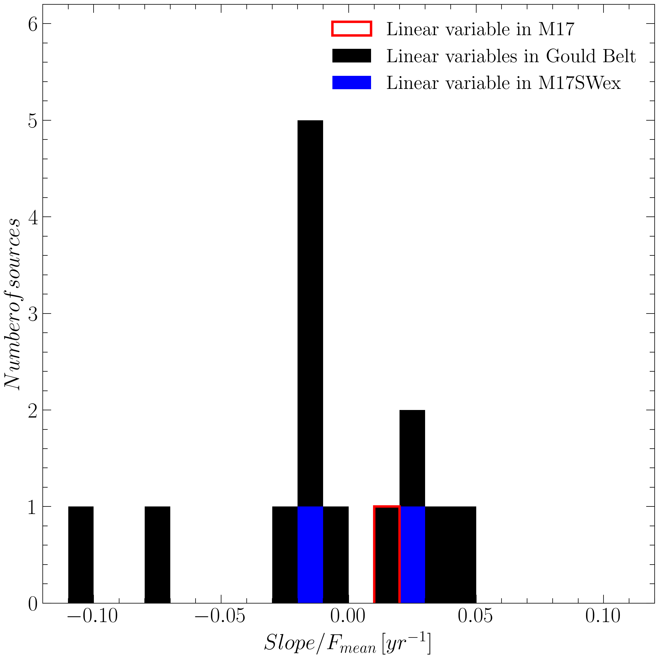
Figure 15: Histograms of the fractional slopes determined by linear fit. The black and blue histogram shows the slopes of linear variables in the Gould belt and M17 SWex recovered by the JCMT Transient survey, respectively.

4.4 Comparison with other JCMT Transient Survey fields

Initially, eight fields from the Gould Belt were monitored by the JCMT Transient Survey (Herczeg et al., 2017). After four years of observations, Lee et al. (2021) searched for and characterized variability on 295 submillimeter peaks brighter than $0.14\,\mathrm{Jy\,beam^{-1}}$ at $850\,\mu$m from these fields. Eighteen out of 83 protostars in the sample were found to exhibit secular variability at submillimeter wavelength (Lee et al., 2021). Increasing the monitoring time to six years, 18 secular variables were robustly recovered along with an additional 20 candidate variables (Mairs et al., 2024). This underscores the importance of long-term monitoring to uncover secular variability.

In M 17, we identified only one secular variable candidate, out of 164 peaks with $F_{\mathrm{850}}>0.14\,\mathrm{Jy\,beam^{-1}}$. Park et al. (2024) identified two secular variable candidates out of 146 peaks with $F_{\mathrm{850}}>0.1\,\mathrm{Jy\,beam^{-1}}$ in M17 SWex. This corresponds to a lower detection rate than the 18 variables out of 83 protostars within the eight fields of the Gould Belt found by Lee et al. (2021) over a similar timescale. Moreover, the secular variable JCMTPP_J182023.2 varies by only $1.1\%/\mathrm{yr}$ over the 3.5-year monitoring for M 17. With a similar timescale of 4 years, the JCMT monitoring for the Gould Belt uncovered 14 linear variables (Lee et al., 2021) and two linear variables for M17 SWex (Park et al., 2024). Figure 15 compares the fractional change per year in $F_{\mathrm{850}}$ of the 16 robust linear variables in Gould Belt and M17 SWex with that of JCMTPP_J182023.2 in M 17. The absolute linear slope of JCMTPP_J182023.2 is close to the lowest value ($0.96\%$) of the absolute slopes of the 14 robust linear variables found in Gould Belt, but is comparable to the slopes of the two linear variables in M17 SWex at a similar distance.

M 17 is at least four times farther away than the eight fields of Gould Belt within 500 pc. It is worth recognizing challenges of detecting submillimeter variability signatures at much greater distances, where for a fixed JCMT-SCUBA2 beam ($\mathrm{HPBW}\sim 14\farcs 4$ at $850\,\mu$m) the amount of envelope and nearby cloud contributing to the observed peak flux increases significantly and may therefore smooth over the localized variations. As discussed in Section 4.3, the interstellar radiation field might also contribute to the dust temperature in the envelope of a protostar. We found a dust temperature of 20 K for the envelope of JCMTPP_J182023.2 returned by the greybody fit. In contrast, the northern condensation in M17 SW, which is much closer than JCMTPP_J182023.2 to the M 17 H II region, was found to have a dust temperature of 30 K derived also from the graybody fit (Hobson et al., 1993). The closer to the H II region, the higher dust temperature is found. The strong interstellar radiation field from the M 17 H II region might somewhat lower the peak flux variability of the submillimeter sources distributed around the H II region, through its contribution to the envelope temperature (Jørgensen et al., 2006). Thus, combined, the greater distance and stronger interstellar radiation likely combine to reduce the detection rate of secular variables at submillimeter wavelengths for the high-mass star-forming region M 17. An in-depth comparison between distant regions (M 17 complex, S255 and DR21) and the Gould Belt regions will be presented in a separate paper (Wang et al. in prepration). The JCMT Transient survey team is also preparing a summary paper that includes the comparison between the regions observed by the survey.

Our mid-IR analyses of M 17 made use of the WISE/NEOWISE monitoring data from the period of 2010 to 2022 December. From the same WISE/NEOWISE data sets, Park et al. (2024) classified 41 variables at W2 in M17 SWex using the same methods as for M 17. The sample of 41 candidate variable YSOs in M17 SWex almost doubles the sample of 22 candidate variable YSOs classified in M 17. In M17 SWex, $56.1\%$ of the sample are Class I YSOs (Park et al., 2024), however, a somewhat lower fraction, 38.1% of the sample in M 17 are Class I YSOs. This difference between the two regions at similar distances might be attributed to the sequential star formation of the M 17 star-forming complex, with the M 17 H II region older than the infrared dark cloud M17 SWex (Povich et al., 2009; Povich & Whitney, 2010; Povich et al., 2016). For mid-IR variability of the candidate YSOs in M 17, we found consistency with those in M17 SWex (Park et al., 2024) in the relative numbers of variables by evolutionary class and variability type, with a higher fraction of Class I than Class II being variable. However, the overall fraction of variability at both evolutionary stages in M 17 and in M17 SWex (Park et al., 2024) are notably lower than those in the Gould Belt (Park et al., 2021). Such a difference does not mean a higher fraction of YSOs with variability in the Gould Belt than in M 17 and M17 SWex. In fact, only 40% of the initial YSO sample in M 17 (30% for M17 SWex; Park et al. 2024) have high-quality NEOWISE data, in contrast this fraction increases to 80% for the YSO sample in the Gould Belt. The YSO samples in M 17 and M17 SWex are likely more biased towards higher mass and/or later stages, lower mass YSOs at early stages probably escape detection even in the infrared because of the high extinction and large distances of the massive star formation clouds. However, the low completeness of the variable YSOs found in M 17 and M17 SWex hampers a solid comparison of the mass-dependent incidence of mid-IR variability to those of the Gould Belt.

5 Summary

This study presents the first comprehensive attempt to characterize YSO variability at mid-IR and submillimeter wavelengths for the massive star-forming region M 17.

We analyze the 3.5 years JCMT Transient Survey data of monthly cadence and the 9 years NEOWISE W2 data with a cadence of six months. A candidate linear variable at $850\,\mu$m (JCMTPP_J182023.2) is identified, with its fractional slope about 8 times the fractional slope uncertainty. The mid-IR analysis reveals significant variability for 22 YSOs. Consistent with the results from other fields within the JCMT Transient survey, eight Gould Belt fields and M17SWex, a higher fraction of Class I YSOs are variable at mid-IR than Class II YSOs, suggesting increased variability at earlier stages of star formation.

The crossmatch between the JCMT submillimeter sources and mid-IR variables returns seven YSOs with JCMT submillimeter sources, three (M17 MIR, SPICY 81957 and 82001) of which are located within the M 17 H II region. Although the three YSOs exhibit significant mid-IR variability, the corresponding submillimeter sources do not show any observable variability at either $450$ or $850\,\mu$m. The candidate linear variable source JCMTPP_J182023.2 is only visible at wavelengths $\lambda\gtrsim 70\,\mu$m, suggesting that the embedded protostar(s) is (are) in a very early stage. The total mass ($172\,M_{\sun}$) and bolometric luminosity ($698\,L_{\sun}$) of JCMTPP_J182023.2 suggests that the source is in the phase of converting mass into luminosity, in line with the evolutionary path of massive star formation. Compared against other MYSOs exhibiting drastic submillimeter bursts observed with interferometric arrays, the submillimeter flux variation of JCMTPP_J182023.2 if modest, a $4\%$ increase in 3.5 years at $850\,\mu$m. This brightness change suggests a lower limit of $\sim 16\%$ for the potential luminosity burst of JCMTPP_J182023.2.

Compared with previous submillimeter and mid-IR variability analyses in the eight nearby Gould Belt regions, we find an order of magnitude decrease in detectable variability within M 17, which is even lower than that within M17 SWex, a more quiescent region at a similar distance. We expect that observing inherent submillimeter and mid-IR variability is more difficult for sources at larger distances and in more complex environments. Our study underscores the necessity of long-term, multi-wavelength monitoring campaigns across a variety of star formation environments to unravel the intricate processes governing the early evolution of YSOs.

For completeness, the locations, peak brightnesses, and variability measures used in this paper for all the bright sources found by the Fellwalker algorithm at $450$ and $850\,\mu$m are presented in Tables 4 and 5, respectively. In Table 6 we list the mid-IR variability measures of the 22 YSOs identified as exhibiting robust mid-IR variability across the six investigated types.

Table 4: JCMT Transient Statistics of Bright Sources ($>0.65\,\mathrm{Jy\,beam^{-1}}$ at $450\,\mu$m) in M 17

Index	ID	$\langle F_{450}\rangle$	$\mathrm{SD}$	$\mathrm{SD/SD_{fid}}$
		($\mathrm{mJy\,bm^{-1}}$)	($\mathrm{mJy\,bm^{-1}}$)
1	JCMTPP_J182022.4-161128	73765	1375	0.7
2	JCMTPP_J182022.7-161156	70575	1161	0.6
3	JCMTPP_J182023.8-161140	67712	1451	0.8
4	JCMTPP_J182021.1-161234	66886	1492	0.8
5	JCMTPP_J182021.5-161252	61609	2184	1.3
6	JCMTPP_J182022.9-161230	50367	1264	0.9
7	JCMTPP_J182018.8-161126	43181	936	0.8
8	JCMTPP_J182024.3-161326	43425	1217	1.0
9	JCMTPP_J182022.6-161258	42492	1417	1.2
10	JCMTPP_J182019.4-161228	40712	1362	1.2
11	JCMTPP_J182023.6-161254	38922	1300	1.2
12	JCMTPP_J182025.1-161350	31763	791	0.9
13	JCMTPP_J182023.3-161448	30173	566	0.7

Note. — Table 4 is published in its entirety in the electronic edition. A portion is shown here for guidance on its form and content.

Table 5: JCMT Transient Statistics of Bright Sources ($>0.14\,\mathrm{Jy\,beam^{-1}}$ at $850\,\mu$m) in M 17

Index	ID	$\langle F_{850}\rangle$	$\mathrm{SD}$	$\mathrm{SD/SD_{fid}}$
		($\mathrm{mJy\,bm^{-1}}$)	($\mathrm{mJy\,bm^{-1}}$)
1	JCMTPP_J182022.4-161127	17954	181	0.8
2	JCMTPP_J182022.8-161154	15409	180	0.9
3	JCMTPP_J182023.6-161139	14873	233	1.2
4	JCMTPP_J182022.8-161012	929	31	1.6
5	JCMTPP_J182030.7-161051	546	17	1.0
6	JCMTPP_J182035.5-161127	311	15	1.0
7	JCMTPP_J182041.5-161148	229	18	1.2
8	JCMTPP_J182021.1-161236	13166	166	1.0
9	JCMTPP_J182022.6-161230	10057	185	1.4
10	JCMTPP_J182024.3-161324	8798	81	0.7
112	JCMTPP_J182023.2-161448	5831	79	1.0

Note. — Table 5 is published in its entirety in the electronic edition. A portion is shown here for guidance on its form and content.

Table 6: Variability Statistics of YSO Candidates in M 17

#	Alias	R.A. (deg)	Decl. (deg)	$\mathrm{N_{W2}}$	Class	$\mathrm{SD}/\sigma$	$\Delta\mathrm{W2}$	$\mathrm{FAP_{LSP}}$	Period	$\mathrm{FAP_{LIN}}$	Slope	Type
		(J2000)	(J2000)				(mag)		(day)		(%/yr)
1	SPICY 81172	274.80060	-16.16145	19	II	1.97	0.26	4.83e-03	2957.9	7.32e-02	-3.15	curved
2	SPICY 81351	274.84851	-16.30373	19	II	4.08	1.10	-	-	-	-	irregular
3	SPICY 81362	274.85173	-16.12506	19	II	2.27	0.31	4.13e-05	3660.3	1.59e-04	5.59	curved
4	SPICY 81397	274.86728	-16.06855	19	II	0.99	0.17	6.02e-03	3660.3	4.12e-03	1.97	curved
5	SPICY 81623	274.96089	-15.91883	19	I	3.76	0.75	2.46e-03	4800.0	2.81e-03	-7.22	curved
6	SPICY 81642	274.97296	-15.93737	19	un.	1.63	0.66	1.15e-03	437.8	6.70e-01	0.98	periodic
7	SPICY 81671	274.98976	-16.20139	19	II	2.29	0.34	2.17e-06	4800.0	3.03e-06	6.17	linear
8	SPICY 81681	274.99467	-16.19189	19	I	3.41	2.37	1.40e-04	247.7	9.98e-01	-0.12	periodic
9	SPICY 81687	274.99663	-16.03847	19	I	2.25	0.67	-	-	-	-	burst
10	SPICY 81696	275.00495	-16.04284	19	I	1.01	0.18	3.75e-03	2481.7	8.01e-01	0.45	periodic
11	SPICY 81724	275.01634	-16.04341	19	un.	1.48	0.44	1.96e-03	4800.0	1.12e-04	-3.75	curved
12	SPICY 81777	275.03838	-16.06545	19	II	5.01	1.36	4.74e-04	232.8	3.48e-01	-4.58	periodic
13	SPICY 81896	275.10147	-15.94373	19	II	2.20	0.59	-	-	-	-	burst
14	SPICY 81925	275.11978	-16.08311	19	II	2.01	0.75	-	-	-	-	burst
15	SPICY 81957	275.13680	-16.02584	19	I	1.70	0.89	7.85e-04	2957.7	9.67e-05	5.51	linear
16	SPICY 81974	275.14552	-16.02265	19	I	1.17	0.25	2.29e-03	4800.0	3.51e-01	1.11	curved
17	SPICY 81998	275.15714	-16.33176	19	II	1.54	0.62	9.00e-03	383.3	2.43e-02	-2.19	periodic
18	SPICY 82001	275.15779	-16.02748	13	un.	3.90	1.01	-	-	-	-	irregular
19	SPICY 82007	275.16341	-15.99153	19	II	5.86	0.95	2.47e-04	403.3	2.71e-02	-10.11	periodic
20	SPICY 82165	275.25569	-15.99572	19	II	3.16	0.50	-	-	-	-	irregular
21	SPICY 82315	275.33538	-16.12251	19	I	3.28	1.00	-	-	-	-	irregular
22	M17 MIR	275.09586	-16.19659	20	I	6.69	2.13	-	-	8.28e-06	7.32	irregular

References

- Astropy Collaboration et al. (2013) Astropy Collaboration, Robitaille, T. P., Tollerud, E. J., et al. 2013, A&A, 558, A33, doi: 10.1051/0004-6361/201322068
- Astropy Collaboration et al. (2018) Astropy Collaboration, Price-Whelan, A. M., Sipőcz, B. M., et al. 2018, AJ, 156, 123, doi: 10.3847/1538-3881/aabc4f
- Audard et al. (2014) Audard, M., Ábrahám, P., Dunham, M. M., et al. 2014, in Protostars and Planets VI, ed. H. Beuther, R. S. Klessen, C. P. Dullemond, & T. Henning, 387–410, doi: 10.2458/azu_uapress_9780816531240-ch017
- Bae et al. (2014) Bae, J., Hartmann, L., Zhu, Z., & Nelson, R. P. 2014, ApJ, 795, 61, doi: 10.1088/0004-637X/795/1/61
- Baek et al. (2020) Baek, G., MacFarlane, B. A., Lee, J.-E., et al. 2020, ApJ, 895, 27, doi: 10.3847/1538-4357/ab8ad4
- Baluev (2008) Baluev, R. V. 2008, MNRAS, 385, 1279, doi: 10.1111/j.1365-2966.2008.12689.x
- Baraffe et al. (2009) Baraffe, I., Chabrier, G., & Gallardo, J. 2009, ApJ, 702, L27, doi: 10.1088/0004-637X/702/1/L27
- Baraffe et al. (2012) Baraffe, I., Vorobyov, E., & Chabrier, G. 2012, ApJ, 756, 118, doi: 10.1088/0004-637X/756/2/118
- Berry (2015) Berry, D. S. 2015, Astronomy and Computing, 10, 22, doi: 10.1016/j.ascom.2014.11.004
- Berry et al. (2007) Berry, D. S., Reinhold, K., Jenness, T., & Economou, F. 2007, in Astronomical Society of the Pacific Conference Series, Vol. 376, Astronomical Data Analysis Software and Systems XVI, ed. R. A. Shaw, F. Hill, & D. J. Bell, 425
- Breen & Ellingsen (2011) Breen, S. L., & Ellingsen, S. P. 2011, MNRAS, 416, 178, doi: 10.1111/j.1365-2966.2011.19020.x
- Burns et al. (2020) Burns, R. A., Sugiyama, K., Hirota, T., et al. 2020, Nature Astronomy, 4, 506, doi: 10.1038/s41550-019-0989-3
- Burns et al. (2023) Burns, R. A., Uno, Y., Sakai, N., et al. 2023, Nature Astronomy, 7, 557, doi: 10.1038/s41550-023-01899-w
- Caratti o Garatti et al. (2017) Caratti o Garatti, A., Stecklum, B., Garcia Lopez, R., et al. 2017, Nature Physics, 13, 276, doi: 10.1038/nphys3942
- Casey (2012) Casey, C. M. 2012, MNRAS, 425, 3094, doi: 10.1111/j.1365-2966.2012.21455.x
- Chapin et al. (2013) Chapin, E. L., Berry, D. S., Gibb, A. G., et al. 2013, MNRAS, 430, 2545, doi: 10.1093/mnras/stt052
- Chen et al. (2020) Chen, X., Sobolev, A. M., Ren, Z.-Y., et al. 2020, Nature Astronomy, 4, 1170, doi: 10.1038/s41550-020-1144-x
- Chen et al. (2012) Chen, Z., Jiang, Z., Wang, Y., et al. 2012, PASJ, 64, 110, doi: 10.1093/pasj/64.5.110
- Chen et al. (2013) Chen, Z., Nürnberger, D. E. A., Chini, R., et al. 2013, A&A, 557, A51, doi: 10.1051/0004-6361/201321694
- Chen et al. (2021) Chen, Z., Sun, W., Chini, R., et al. 2021, ApJ, 922, 90, doi: 10.3847/1538-4357/ac2151
- Chibueze et al. (2016) Chibueze, J. O., Kamezaki, T., Omodaka, T., et al. 2016, MNRAS, 460, 1839, doi: 10.1093/mnras/stw1019
- Contreras Peña et al. (2020) Contreras Peña, C., Johnstone, D., Baek, G., et al. 2020, MNRAS, 495, 3614, doi: 10.1093/mnras/staa1254
- Contreras Peña et al. (2017) Contreras Peña, C., Lucas, P. W., Minniti, D., et al. 2017, MNRAS, 465, 3011, doi: 10.1093/mnras/stw2801
- Covey et al. (2021) Covey, K. R., Larson, K. A., Herczeg, G. J., & Manara, C. F. 2021, AJ, 161, 61, doi: 10.3847/1538-3881/abcc73
- Currie et al. (2014) Currie, M. J., Berry, D. S., Jenness, T., et al. 2014, in Astronomical Society of the Pacific Conference Series, Vol. 485, Astronomical Data Analysis Software and Systems XXIII, ed. N. Manset & P. Forshay, 391
- De Buizer et al. (2005) De Buizer, J. M., Radomski, J. T., Telesco, C. M., & Piña, R. K. 2005, ApJS, 156, 179, doi: 10.1086/426941
- Di Francesco et al. (2008) Di Francesco, J., Johnstone, D., Kirk, H., MacKenzie, T., & Ledwosinska, E. 2008, ApJS, 175, 277, doi: 10.1086/523645
- Drew et al. (2014) Drew, J. E., Gonzalez-Solares, E., Greimel, R., et al. 2014, MNRAS, 440, 2036, doi: 10.1093/mnras/stu394
- Fischer et al. (2023) Fischer, W. J., Hillenbrand, L. A., Herczeg, G. J., et al. 2023, in Astronomical Society of the Pacific Conference Series, Vol. 534, Protostars and Planets VII, ed. S. Inutsuka, Y. Aikawa, T. Muto, K. Tomida, & M. Tamura, 355, doi: 10.48550/arXiv.2203.11257
- Fischer et al. (2024) Fischer, W. J., Battersby, C., Johnstone, D., et al. 2024, AJ, 167, 82, doi: 10.3847/1538-3881/ad188b
- Francis et al. (2022) Francis, L., Johnstone, D., Lee, J.-E., et al. 2022, ApJ, 937, 29, doi: 10.3847/1538-4357/ac8a9e
- Furuya et al. (2005) Furuya, R. S., Kitamura, Y., Wootten, A., Claussen, M. J., & Kawabe, R. 2005, A&A, 438, 571, doi: 10.1051/0004-6361:20034189
- Herczeg et al. (2017) Herczeg, G. J., Johnstone, D., Mairs, S., et al. 2017, ApJ, 849, 43, doi: 10.3847/1538-4357/aa8b62
- Hill et al. (2005) Hill, T., Burton, M. G., Minier, V., et al. 2005, MNRAS, 363, 405, doi: 10.1111/j.1365-2966.2005.09347.x
- Hirota et al. (2022) Hirota, T., Wolak, P., Hunter, T. R., et al. 2022, PASJ, 74, 1234, doi: 10.1093/pasj/psac067
- Hobson et al. (1993) Hobson, M. P., Padman, R., Scott, P. F., Prestage, R. M., & Ward-Thompson, D. 1993, MNRAS, 264, 1025, doi: 10.1093/mnras/264.4.1025
- Hodapp et al. (2019) Hodapp, K. W., Reipurth, B., Pettersson, B., et al. 2019, AJ, 158, 241, doi: 10.3847/1538-3881/ab471a
- Hoffmeister et al. (2008) Hoffmeister, V. H., Chini, R., Scheyda, C. M., et al. 2008, ApJ, 686, 310, doi: 10.1086/591070
- Holland et al. (2013) Holland, W. S., Bintley, D., Chapin, E. L., et al. 2013, MNRAS, 430, 2513, doi: 10.1093/mnras/sts612
- Hunter et al. (2017) Hunter, T. R., Brogan, C. L., MacLeod, G., et al. 2017, ApJ, 837, L29, doi: 10.3847/2041-8213/aa5d0e
- Hunter et al. (2021) Hunter, T. R., Brogan, C. L., De Buizer, J. M., et al. 2021, ApJ, 912, L17, doi: 10.3847/2041-8213/abf6d9
- Jaffe et al. (1981) Jaffe, D. T., Guesten, R., & Downes, D. 1981, ApJ, 250, 621, doi: 10.1086/159409
- Johnstone et al. (2013) Johnstone, D., Hendricks, B., Herczeg, G. J., & Bruderer, S. 2013, ApJ, 765, 133, doi: 10.1088/0004-637X/765/2/133
- Johnstone et al. (2018) Johnstone, D., Herczeg, G. J., Mairs, S., et al. 2018, ApJ, 854, 31, doi: 10.3847/1538-4357/aaa764
- Jørgensen et al. (2006) Jørgensen, J. K., Johnstone, D., van Dishoeck, E. F., & Doty, S. D. 2006, A&A, 449, 609, doi: 10.1051/0004-6361:20053011
- Kackley et al. (2010) Kackley, R., Scott, D., Chapin, E., & Friberg, P. 2010, in Society of Photo-Optical Instrumentation Engineers (SPIE) Conference Series, Vol. 7740, Software and Cyberinfrastructure for Astronomy, ed. N. M. Radziwill & A. Bridger, 77401Z, doi: 10.1117/12.857397
- Kenyon et al. (1990) Kenyon, S. J., Hartmann, L. W., Strom, K. M., & Strom, S. E. 1990, AJ, 99, 869, doi: 10.1086/115380
- Kóspál et al. (2007) Kóspál, Á., Ábrahám, P., Prusti, T., et al. 2007, A&A, 470, 211, doi: 10.1051/0004-6361:20066108
- Kuhn et al. (2021) Kuhn, M. A., de Souza, R. S., Krone-Martins, A., et al. 2021, ApJS, 254, 33, doi: 10.3847/1538-4365/abe465
- Kuhn et al. (2019) Kuhn, M. A., Hillenbrand, L. A., Sills, A., Feigelson, E. D., & Getman, K. V. 2019, ApJ, 870, 32, doi: 10.3847/1538-4357/aaef8c
- Kunitomo et al. (2017) Kunitomo, M., Guillot, T., Takeuchi, T., & Ida, S. 2017, A&A, 599, A49, doi: 10.1051/0004-6361/201628260
- Lee et al. (2024) Lee, S., Lee, J.-E., Contreras Peña, C., et al. 2024, ApJ, 962, 38, doi: 10.3847/1538-4357/ad14f8
- Lee et al. (2020) Lee, Y.-H., Johnstone, D., Lee, J.-E., et al. 2020, ApJ, 903, 5, doi: 10.3847/1538-4357/abb6fe
- Lee et al. (2021) —. 2021, ApJ, 920, 119, doi: 10.3847/1538-4357/ac1679
- Lim et al. (2020) Lim, W., De Buizer, J. M., & Radomski, J. T. 2020, ApJ, 888, 98, doi: 10.3847/1538-4357/ab5fd0
- Lin et al. (2021) Lin, Z.-Y. D., Lee, C.-F., Li, Z.-Y., Tobin, J. J., & Turner, N. J. 2021, MNRAS, 501, 1316, doi: 10.1093/mnras/staa3685
- Liu et al. (2018) Liu, S.-Y., Su, Y.-N., Zinchenko, I., Wang, K.-S., & Wang, Y. 2018, ApJ, 863, L12, doi: 10.3847/2041-8213/aad63a
- Lomb (1976) Lomb, N. R. 1976, Ap&SS, 39, 447, doi: 10.1007/BF00648343
- MacFarlane et al. (2019a) MacFarlane, B., Stamatellos, D., Johnstone, D., et al. 2019a, MNRAS, 487, 4465, doi: 10.1093/mnras/stz1570
- MacFarlane et al. (2019b) —. 2019b, MNRAS, 487, 5106, doi: 10.1093/mnras/stz1512
- Mainzer et al. (2011) Mainzer, A., Bauer, J., Grav, T., et al. 2011, ApJ, 731, 53, doi: 10.1088/0004-637X/731/1/53
- Mainzer et al. (2014) Mainzer, A., Bauer, J., Cutri, R. M., et al. 2014, ApJ, 792, 30, doi: 10.1088/0004-637X/792/1/30
- Mairs et al. (2017a) Mairs, S., Lane, J., Johnstone, D., et al. 2017a, ApJ, 843, 55, doi: 10.3847/1538-4357/aa7844
- Mairs et al. (2017b) Mairs, S., Johnstone, D., Kirk, H., et al. 2017b, ApJ, 849, 107, doi: 10.3847/1538-4357/aa9225
- Mairs et al. (2021) Mairs, S., Dempsey, J. T., Bell, G. S., et al. 2021, AJ, 162, 191, doi: 10.3847/1538-3881/ac18bf
- Mairs et al. (2024) Mairs, S., Lee, S., Johnstone, D., et al. 2024, ApJ, 966, 215, doi: 10.3847/1538-4357/ad35b6
- Ma´ız Apellániz et al. (2022) Maíz Apellániz, J., Barbá, R. H., Fernández Aranda, R., et al. 2022, A&A, 657, A131, doi: 10.1051/0004-6361/202142364
- McMullin et al. (2007) McMullin, J. P., Waters, B., Schiebel, D., Young, W., & Golap, K. 2007, in Astronomical Society of the Pacific Conference Series, Vol. 376, Astronomical Data Analysis Software and Systems XVI, ed. R. A. Shaw, F. Hill, & D. J. Bell, 127
- Megeath et al. (2012) Megeath, S. T., Gutermuth, R., Muzerolle, J., et al. 2012, AJ, 144, 192, doi: 10.1088/0004-6256/144/6/192
- Meyer et al. (2019) Meyer, D. M. A., Vorobyov, E. I., Elbakyan, V. G., et al. 2019, MNRAS, 482, 5459, doi: 10.1093/mnras/sty2980
- Molinari et al. (2008) Molinari, S., Pezzuto, S., Cesaroni, R., et al. 2008, A&A, 481, 345, doi: 10.1051/0004-6361:20078661
- Moscadelli et al. (2013) Moscadelli, L., Li, J. J., Cesaroni, R., et al. 2013, A&A, 549, A122, doi: 10.1051/0004-6361/201220497
- Nagel & Bouvier (2019) Nagel, E., & Bouvier, J. 2019, A&A, 625, A45, doi: 10.1051/0004-6361/201833979
- Nguyen-Luong et al. (2020) Nguyen-Luong, Q., Nakamura, F., Sugitani, K., et al. 2020, ApJ, 891, 66, doi: 10.3847/1538-4357/ab700a
- Park et al. (2019) Park, G., Kim, K.-T., Johnstone, D., et al. 2019, ApJS, 242, 27, doi: 10.3847/1538-4365/ab1eae
- Park et al. (2024) Park, G., Johnstone, D., Peña, C. C., et al. 2024, AJ, 168, 122, doi: 10.3847/1538-3881/ad5e6e
- Park et al. (2021) Park, W., Lee, J.-E., Contreras Peña, C., et al. 2021, ApJ, 920, 132, doi: 10.3847/1538-4357/ac1745
- Poglitsch et al. (2010) Poglitsch, A., Waelkens, C., Geis, N., et al. 2010, A&A, 518, L2, doi: 10.1051/0004-6361/201014535
- Povich et al. (2016) Povich, M. S., Townsley, L. K., Robitaille, T. P., et al. 2016, ApJ, 825, 125, doi: 10.3847/0004-637X/825/2/125
- Povich & Whitney (2010) Povich, M. S., & Whitney, B. A. 2010, ApJ, 714, L285, doi: 10.1088/2041-8205/714/2/L285
- Povich et al. (2009) Povich, M. S., Churchwell, E., Bieging, J. H., et al. 2009, ApJ, 696, 1278, doi: 10.1088/0004-637X/696/2/1278
- Povich et al. (2013) Povich, M. S., Kuhn, M. A., Getman, K. V., et al. 2013, ApJS, 209, 31, doi: 10.1088/0067-0049/209/2/31
- Reid & Wilson (2006) Reid, M. A., & Wilson, C. D. 2006, ApJ, 644, 990, doi: 10.1086/503824
- Safron et al. (2015) Safron, E. J., Fischer, W. J., Megeath, S. T., et al. 2015, ApJ, 800, L5, doi: 10.1088/2041-8205/800/1/L5
- Scargle (1989) Scargle, J. D. 1989, ApJ, 343, 874, doi: 10.1086/167757
- Scholz et al. (2013) Scholz, A., Froebrich, D., & Wood, K. 2013, MNRAS, 430, 2910, doi: 10.1093/mnras/stt091
- Scholz et al. (2015) Scholz, A., Mužić, K., & Geers, V. 2015, MNRAS, 451, 26, doi: 10.1093/mnras/stv838
- Sheehan et al. (2025) Sheehan, P. D., Johnstone, D., Contreras Peña, C., et al. 2025, ApJ, 982, 176, doi: 10.3847/1538-4357/adaf9b
- Stecklum et al. (2021) Stecklum, B., Wolf, V., Linz, H., et al. 2021, A&A, 646, A161, doi: 10.1051/0004-6361/202039645
- Stoop et al. (2024) Stoop, M., Derkink, A., Kaper, L., et al. 2024, A&A, 681, A21, doi: 10.1051/0004-6361/202347383
- Taylor (2005) Taylor, M. B. 2005, in Astronomical Society of the Pacific Conference Series, Vol. 347, Astronomical Data Analysis Software and Systems XIV, ed. P. Shopbell, M. Britton, & R. Ebert, 29
- Urquhart et al. (2022) Urquhart, J. S., Wells, M. R. A., Pillai, T., et al. 2022, MNRAS, 510, 3389, doi: 10.1093/mnras/stab3511
- Vorobyov & Basu (2015) Vorobyov, E. I., & Basu, S. 2015, ApJ, 805, 115, doi: 10.1088/0004-637X/805/2/115
- Wenner et al. (2022) Wenner, N., Sarma, A. P., & Momjian, E. 2022, ApJ, 930, 114, doi: 10.3847/1538-4357/ac625c
- WISE Team (2020) WISE Team. 2020, NEOWISE 2-Band Post-Cryo Single Exposure (L1b) Source Table, NASA IPAC DataSet, IRSA124, doi: 10.26131/IRSA124
- Wolf et al. (2024) Wolf, V., Stecklum, B., Caratti o Garatti, A., et al. 2024, A&A, 688, A8, doi: 10.1051/0004-6361/202449891
- Wolk et al. (2018) Wolk, S. J., Günther, H. M., Poppenhaeger, K., et al. 2018, AJ, 155, 99, doi: 10.3847/1538-3881/aaa6c4
- Wright et al. (2010) Wright, E. L., Eisenhardt, P. R. M., Mainzer, A. K., et al. 2010, AJ, 140, 1868, doi: 10.1088/0004-6256/140/6/1868
- Wright et al. (2019) —. 2019, AllWISE Source Catalog, NASA IPAC DataSet, IRSA1, doi: 10.26131/IRSA1
- Xu et al. (2011) Xu, Y., Moscadelli, L., Reid, M. J., et al. 2011, ApJ, 733, 25, doi: 10.1088/0004-637X/733/1/25
- Yin et al. (2021) Yin, J., Chen, Z., Chini, R., et al. 2021, AJ, 162, 52, doi: 10.3847/1538-3881/abfdcd
- Yoo et al. (2017) Yoo, H., Lee, J.-E., Mairs, S., et al. 2017, ApJ, 849, 69, doi: 10.3847/1538-4357/aa8c0a
- Zakri et al. (2022) Zakri, W., Megeath, S. T., Fischer, W. J., et al. 2022, ApJ, 924, L23, doi: 10.3847/2041-8213/ac46ae
- Zhou et al. (2024) Zhou, W., Chen, Z., Jiang, Z., Feng, H., & Jiang, Y. 2024, ApJ, 969, L6, doi: 10.3847/2041-8213/ad55c7