Learning event-triggered controllers for linear parameter-varying systems from data

Abstract

Nonlinear dynamical behaviours in engineering applications can be approximated by linear-parameter varying (LPV) representations, but obtaining precise model knowledge to develop a control algorithm is difficult in practice. In this paper, we develop the data-driven control strategies for event-triggered LPV systems with stability verifications. First, we provide the theoretical analysis of $\theta$-persistence of excitation for LPV systems, which leads to the feasible data-based representations. Then, in terms of the available perturbed data, we derive the stability certificates for event-triggered LPV systems with the aid of Petersen’s lemma in the sense of robust control, resulting in the computationally tractable semidefinite programmings, the feasible solutions of which yields the optimal gain schedulings. Besides, we generalize the data-driven event-triggered LPV control methods to the scenario of reference trajectory tracking, and discuss the robust tracking stability accordingly. Finally, we verify the effectiveness of our theoretical derivations by numerical simulations.

Data-driven control, persistence of excitation, linear parameter-varying system, event-triggered control, convex optimization.

1 Introduction

Complex dynamical systems in engineering applications, for example, hypersonic aircrafts, autonomous vehicles, as well as turbofan engines, are intrinsically with nonlinear attributes [1]. There exist difficulties in analysis and control of such systems, by virtue of computationally tractable tools from linear time-invariant framework. Within this context, linear parameter-varying (LPV) representations, formulated by a linear system with time-varying scheduling signals, which embed nonlinear and/or uncertain impacts, can be utilized to address the issues of providing the theoretical guarantees on system performance [2]. However, obtaining model knowledge of LPV systems via first-principle analysis or system identification needs heavy computation burdens and lacks theoretical supports for control synthesis. Hence, the needs of developing control strategies of LPV systems directly from data, that can bypass a complex modeling process, are with far-reaching meanings.

1.1 Related Literature

Allowing for the measurable and time-varying scheduling signals within bounded convex sets, LPV systems approximate the linear input-output relationships of nonlinear processes [3]. Note that such scheduling signal of a certain LPV system can be only achieved at the current instant but unknown afterwards, thus, LPV synthesis aims to develop a control strategy of the same structure, such that the closed-loop performances are guaranteed over the entire set of permissible scheduling signals [4]. The use of quadratic Lyapunov functions, which are affine in the scheduling signal, leads to the robust stability certificate in terms of linear matrix inequalities (LMIs) [4]. Normally, the scheduling signals are assumed to perform the bounded parameter variations [5] and the bounded rates of variations [6]. There exists a compromise between computation tractability and representation power for LPV systems [7]. The closed-loop performance guarantees can lead to an infinite number of LMIs, which are hard to find the feasible solutions for control synthesis. Hence, the relaxation techniques are preferred for computationally tractable control algorithms, for example, convex-hull relaxation [8], partial-convexity approach [6], grid partition argument [9], Finsler’s lemma and affine annihilators relaxation [10], and slack variable method [11], to name a few. Apart from high computational demands induced by a large number of decision parameters, which are incorporated in these convex programmings with quadratic performance certificates, reducing conservatism of LPV performance analysis needs to be considered [13], since the conservative methods can lead to ill-conditioning and fail to find a feasible solution for gain scheduling. Owing to the developments of aperiodic-sampling communication transmissions, developing event-triggered LPV controller to refine communication efficiency, on the premise of closed-loop performance guarantees, has attracted research attentions in recent years [12]. The existing results depend on the LPV model knowledge, how to develop an event-triggered LPV controller directly from data, when the model knowledge is unavailable, remains an open issue to be further investigated.

Based on the Willems fundamental lemma of persistence of excitation [14, 15, 16], the parameterization of linear feedback systems from data pushes forward the developments of data-dependent control algorithms, in which explicit system identifications are not required [17]. The critical problem lies in involving the data-based performance verifications in the control algorithms, for example, linear quadratic regulator [18] and model predictive control [19]. It is noteworthy that the inevitable presence of external perturbations in data and/or physical plant, such as noise and disturbance [20, 21, 22, 23], leads to the nonequivalent representation of actual systems. For the specific bound on perturbation, a set of systems cannot distinguish from each other in terms of the available data. The data batches are obtained within the context of open-loop experiments and then used for control synthesis [24], that targets all systems described by the same data-based representation. This issue motivates one of the main research lines of data-driven control in recent years. By virtue of linear fractional transformation [25], full-block matrix S-lemma [26], Petersen’s lemma [27], Young’s inequality relaxation [28], and Farkas’s lemma [29], data-dependent performance certificates of closed-loop systems can be obtained, leading to either semi-definite programmings or sum-of-squares programmings, and the feasibility of which implies an available data-driven control strategy. This methodology has been widely utilized to handle dissipativity analysis [30], reachability assessment [31], online switching mechanism specification [24], transfer stabilization [32], Koopman-based feedback design [33], integral quadratic constraint-based argument [34], performances assurance [35], and observer development [36]. Moreover, aperiodic sampling-based communication transmissions can be incorporated into data-driven control algorithms, in which the time span between adjacent sampling instants is maximized by a user-defined triggering logic while preserving the closed-loop performance, leading to the innovative data-based event-triggered controller [37] and self-triggered controller [40], holding for linear time-invariant systems. Albeit data-driven approaches can successfully be applied to LPV systems, in terms of input-scheduling-state/output data, to cope with the dissipativity analysis based on Finsler’s lemma [41] and the LPV control gain scheduling [42], fewer results have investigated the event-triggered control design for perturbed LPV systems from data and have extracted the $\theta$-persistence of excitation prerequisite for data-driven control of LPV systems, which leave the room for further study.

1.2 Technical Contributions

In this paper, we establish the event-triggered control strategies for perturbed LPV systems from data, in order to fill the gap between aperiodic-sampling communication transmissions and data-driven LPV control. For the perturbed LPV systems, the existing persistence of excitation argument of linear time-invariant framework [46] is not applicable, such issue has not been thoroughly revealed in the innovative result [41]. Although the recent work [43] has generalized the Willems fundamental lemma to the LPV framework, the kernel-based representation cannot be directly applied to data-driven control synthesis, and only the shifted-affine scheduling signal is considered therein. Besides, the data-based stability analysis and control synthesis herein are different from the existing work [42], allowing for the deployed event-triggered communication mechanisms with the channel from controller to actuator and the perturbed LPV systems. The Petersen’s lemma and the full-block S-procedure are utilized to derive the semidefinite programmings solvable at the vertices of polytopic set of scheduling signal as adopted in the model-based approaches [44]. To some extent, we make an effort to extend the methodology of learning event-triggered control of linear time-invariant systems [37, 38, 39] to LPV systems. Moreover, the existing literature about data-driven LPV control cannot cope with the robust output tracking issue directly, and in terms of the auxiliary integral compensator technique [45], we accordingly develop a learning event-triggered controller for LPV output tracking. The main contributions of this paper can be briefly summarized by the following keypoints.
$\bullet$ The $\theta$-persistence of excitation condition for LPV systems is explored for the first time, which reveals the smallest value of the length of collected data and acts as the prerequisite for data-driven analysis and control of perturbed LPV systems.
$\bullet$ The sufficient conditions for ensuring the closed-loop stability of perturbed LPV systems, in view of data-based representation, are derived by Petersen’s lemma and full-block S-procedure, leading to the computationally tractable convex programming, feasible at the vertices of the polytopic set of scheduling signal, such that data-based LPV control synthesis is promising.
$\bullet$ With the deployment of event-triggered communication transmissions in the controller-to-actuator channel, we establish the relationships between the stability certificate and the triggering parameters. Solving the data-based convex programming leads to the potentials of event-triggered LPV control synthesis from available data.
$\bullet$ We extend the theoretical results to the scenario of reference tracking. By introducing the auxiliary integral compensator, we can construct an augmented LPV systems and then can establish the corresponding stability certificates, yielding the solvable data-dependent convex programmings, to develop the event-triggered LPV tracking controller.

1.3 Outline of This Paper

The problem formulation and preliminaries with respect to robust data-driven control of perturbed LPV systems are stated in Section 2. The stability verification of LPV systems and the data-driven event-triggered LPV control synthesis for both the stabilization and the output tracking scenarios are discussed in Section 3. We perform the numerical simulations to verify the effectiveness of theoretical derivations in Section 4, and conclude this paper in Section 5.

1.4 Applicatory Notations

Most of the applicatory notations are standard, therefore, we only introduce the specific ones to be utilized herein. $\mathds{N}_{[\ell_{1},\ell_{2}]}$ represents the integer set $\{\ell_{1},\ell_{1}\hskip-1.99997pt+\hskip-1.99997pt1,\cdots\hskip-1.99997pt,\ell_{2}\}$. $\mathds{R}_{+}$ and $\mathds{N}_{+}$ imply the positive real number and integer sets, respectively. Besides, $\mathbb{S}^{n}(\mathbb{S}_{++}^{n})$ is the set of (positive) symmetrical square matrices. The Kronecker product of $M\hskip-3.00003pt\in\hskip-3.00003pt\mathds{R}^{m\times n}$ and $N\hskip-3.00003pt\in\hskip-3.00003pt\mathds{R}^{p\times q}$ is denoted by $M\hskip-1.99997pt\otimes\hskip-1.99997ptN\hskip-3.00003pt\in\hskip-3.00003pt\mathds{R}^{mp\times nq}$. The operator $\mathrm{Col}(X_{1},\cdots\hskip-1.99997pt,X_{\ell})$ with $\ell\hskip-1.99997pt\in\mathds{N}_{+}$ denotes an augmented column vector/matrix, in which $X_{\imath}$, $\imath\hskip-1.99997pt\in\hskip-1.99997pt\mathds{N}_{[1,\ell]}$ is with suitable dimension. $\mathrm{Blkdiag}(x)$ represents a diagonal matrix, each diagonal element of which is the vector $x$, whereas $\hskip-1.00006pt\mathrm{Blkdiag}(X,\hskip-1.00006ptY)$ represents the block-diagonal matrix, the diagonal elements of which are $X$ and $Y$ in sequence. For a matrix $G$, we represent its Moore-Penrose inverse by $G^{\dagger}$ if available. Given a vector $x_{k}$ and time instants $t_{1},t_{2}\hskip-3.00003pt\in\hskip-3.00003pt\mathds{N}_{+}$, we define $\hskip-1.00006pt\|x_{k}\|_{[t_{1},t_{2}]}$ $=\hskip-1.99997pt\sup_{k\in[t_{1},t_{2}]}\hskip-3.00003pt\|x_{k}\|$. For a sequence $\hskip-1.00006pt\{x_{k}\}_{k=0}^{\mathcal{T}-1}$, the Hankel matrix $\boldsymbol{\mathcal{H}}_{L}(x_{[0,\mathcal{T}-1]})$ is denoted by

$$\boldsymbol{\mathcal{H}}_{L}(x_{[0,\mathcal{T}-1]})\hskip-1.99997pt=\hskip-1.99997pt\left[\hskip-1.99997pt\begin{array}[]{cccc}x_{0}\hskip-1.99997pt&\hskip-1.99997ptx_{1}\hskip-1.99997pt&\hskip-1.99997pt\cdots\hskip-1.99997pt&\hskip-1.99997ptx_{\mathcal{T}-L}\\ x_{1}\hskip-1.99997pt&\hskip-1.99997ptx_{2}\hskip-1.99997pt&\hskip-1.99997pt\cdots\hskip-1.99997pt&\hskip-1.99997ptx_{\mathcal{T}-L+1}\\ \vdots\hskip-1.99997pt&\hskip-1.99997pt\vdots\hskip-1.99997pt&\hskip-1.99997pt\ddots\hskip-1.99997pt&\hskip-1.99997pt\vdots\\ x_{L-1}\hskip-1.99997pt&\hskip-1.99997ptx_{L}\hskip-1.99997pt&\hskip-1.99997pt\cdots\hskip-1.99997pt&\hskip-1.99997ptx_{\mathcal{T}-1}\end{array}\hskip-1.99997pt\right].$$

2 Problem Formulation

2.1 System Description

For the sampling instant $k\hskip-1.99997pt\in\hskip-1.99997pt\mathds{N}$, a discrete-time LPV system can be formulated by the state-space representation

$$\hskip-6.00006pt\boldsymbol{x}_{k+1}\hskip-3.00003pt \hskip-6.00006pt=\hskip-6.00006pt \hskip-3.00003ptA_{d}(\boldsymbol{p}_{k})\boldsymbol{x}_{k}\hskip-1.99997pt+\hskip-1.99997ptB_{d}(\boldsymbol{p}_{k})\boldsymbol{u}_{k}\hskip-1.99997pt+\hskip-1.99997pt\boldsymbol{\omega_{k}},$$

$$\hskip-6.00006pt\boldsymbol{y}_{k}\hskip-3.00003pt \hskip-6.00006pt=\hskip-6.00006pt \hskip-3.00003ptC_{d}(\boldsymbol{p}_{k})\boldsymbol{x}_{k}\hskip-1.99997pt+\hskip-1.99997ptD_{d}(\boldsymbol{p}_{k})\boldsymbol{u}_{k},$$ (2)

where $\hskip-1.00006pt\boldsymbol{x}_{k}\hskip-1.99997pt\in\hskip-1.99997pt\mathds{R}^{n}$, $\hskip-1.99997pt\boldsymbol{u}_{k}\hskip-1.99997pt\in\hskip-1.99997pt\mathds{R}^{m}$, $\hskip-1.00006pt\boldsymbol{y}_{k}\hskip-1.99997pt\in\hskip-1.99997pt\mathds{R}^{r}$, $\hskip-1.00006pt\boldsymbol{p}_{k}\hskip-1.99997pt\in\hskip-1.99997pt\mathds{P}$, and $\hskip-1.00006pt\boldsymbol{\omega}_{k}\hskip-1.99997pt\in\hskip-1.99997pt\mathds{R}^{n}\hskip-1.00006pt$ capture the system state, controlled input, measured output, scheduling signal, and external perturbation, respectively. Accordingly, the mappings $\hskip-1.99997ptA_{d}\hskip-1.99997pt:\hskip-1.99997pt\mathds{P}\hskip-3.00003pt\mapsto\hskip-3.00003pt\mathds{R}^{n\times n}$, $\hskip-1.99997ptB_{d}\hskip-1.99997pt:\hskip-1.99997pt\mathds{P}\hskip-3.00003pt\mapsto\hskip-3.00003pt\mathds{R}^{n\times m}$, $\hskip-1.99997ptC_{d}\hskip-1.99997pt:\hskip-1.99997pt\mathds{P}\hskip-3.00003pt\mapsto\hskip-3.00003pt\mathds{R}^{r\times n}$, and $D_{d}\hskip-1.99997pt:\hskip-1.99997pt\mathds{P}\hskip-3.00003pt\mapsto\hskip-3.00003pt\mathds{R}^{r\times m}$ have the affine dependency on $p_{k}$, namely,

$$\hskip-10.00002ptA_{d}(\boldsymbol{p}_{k})\hskip-3.00003pt \hskip-6.00006pt=\hskip-6.00006pt \hskip-3.99994ptA_{d0}\hskip-1.99997pt+\hskip-3.00003pt\sum\limits_{\imath=1}^{\ell}\boldsymbol{p}_{k}^{[\imath]}A_{d\imath},B_{d}(\boldsymbol{p}_{k})\hskip-3.00003pt=\hskip-3.00003ptB_{d0}\hskip-1.99997pt+\hskip-3.00003pt\sum\limits_{\imath=1}^{\ell}\boldsymbol{p}_{k}^{[\imath]}B_{d\imath},$$

$$\hskip-10.00002ptC_{d}(\boldsymbol{p}_{k})\hskip-3.00003pt \hskip-6.00006pt=\hskip-6.00006pt \hskip-3.99994ptC_{d0}\hskip-1.99997pt+\hskip-3.00003pt\sum\limits_{\imath=1}^{\ell}\boldsymbol{p}_{k}^{[\imath]}C_{d\imath},D_{d}(\boldsymbol{p}_{k})\hskip-1.99997pt=\hskip-1.99997ptD_{d0}\hskip-1.99997pt+\hskip-3.00003pt\sum\limits_{\imath=1}^{\ell}\boldsymbol{p}_{k}^{[\imath]}D_{d\imath},$$ (3)

where the matrices $\hskip-1.00006ptA_{d\imath}$, $B_{d\imath}$, $C_{d\imath}$, and $\hskip-1.00006ptD_{d\imath}$ for $\hskip-1.00006pt\imath\hskip-1.99997pt\in\hskip-1.99997pt\mathds{N}_{[0,\ell]}$ are with the appropriate dimensions, and the superscript $[\imath]$ implies the $\imath$-th element of the scheduling signal $\boldsymbol{p}_{k}$. Allowing for the separation of coefficient matrices in (3), we further rewrite the LPV system (2) with the following form

$$\hskip-6.00006pt\boldsymbol{x}_{k+1}\hskip-3.00003pt \hskip-6.00006pt=\hskip-6.00006pt \hskip-3.00003pt\mathcal{A}_{d}\boldsymbol{z}_{k}\hskip-1.99997pt+\hskip-1.99997pt\mathcal{B}_{d}\boldsymbol{\bar{u}}_{k}\hskip-1.99997pt+\hskip-1.99997pt\boldsymbol{\omega}_{k},$$

$$\hskip-6.00006pt\boldsymbol{y}_{k}\hskip-3.00003pt \hskip-6.00006pt=\hskip-6.00006pt \hskip-3.00003pt\mathcal{C}_{d}\boldsymbol{z}_{k}\hskip-1.99997pt+\hskip-1.99997pt\mathcal{D}_{d}\boldsymbol{\bar{u}}_{k},$$ (4)

where $\boldsymbol{z}_{k}\hskip-1.99997pt=\hskip-1.99997pt\mathrm{Col}(\boldsymbol{x}_{k},\boldsymbol{p}_{k}\hskip-1.99997pt\otimes\hskip-1.99997pt\boldsymbol{x}_{k})$, $\boldsymbol{\bar{u}}_{k}\hskip-1.99997pt=\hskip-1.99997pt\mathrm{Col}(\boldsymbol{u_{k}},\boldsymbol{p}_{k}\hskip-1.99997pt\otimes\hskip-1.99997pt\boldsymbol{u}_{k})$, and

$$\hskip-6.00006pt\mathcal{A}_{d}\hskip-3.00003pt \hskip-6.00006pt=\hskip-6.00006pt \hskip-3.00003pt[A_{d0},A_{d1},\cdots,A_{d\ell}],\mathcal{B}_{d}\hskip-1.99997pt=\hskip-3.00003pt[B_{d0},B_{d1},\cdots,B_{d\ell}],$$

$$\hskip-6.00006pt\mathcal{C}_{d}\hskip-3.00003pt \hskip-6.00006pt=\hskip-6.00006pt \hskip-3.00003pt[C_{d0},C_{d1},\cdots,C_{d\ell}],\mathcal{D}_{d}\hskip-1.99997pt=\hskip-3.00003pt[D_{d0},D_{d1},\cdots,D_{d\ell}].$$

We collect the data for the LPV system (4), leading to the data set $\mathbb{D}_{s}\hskip-3.00003pt=\hskip-3.00003pt\{\boldsymbol{u}_{k},\boldsymbol{p}_{k},\boldsymbol{x}_{k},\boldsymbol{\omega}_{k}\}_{k=0}^{\mathcal{T}}$. Therefore, we can construct the following data matrices for a specific time window $\mathcal{T}\hskip-1.99997pt\in\hskip-1.99997pt\mathds{N}_{+}$,

$$\hskip-6.00006pt\boldsymbol{U} \hskip-3.00003pt=\hskip-3.00003pt[\boldsymbol{u}_{0},\cdots,\boldsymbol{u}_{\mathcal{T}-1}]\hskip-1.99997pt\in\hskip-1.99997pt\mathds{R}^{m\times\mathcal{T}}\hskip-1.99997pt,$$ (5a)

$$\hskip-6.00006pt\boldsymbol{U}_{\hskip-1.63885ptP} \hskip-3.00003pt=\hskip-3.00003pt[\boldsymbol{p}_{0}\hskip-1.99997pt\otimes\hskip-1.99997pt\boldsymbol{u}_{0},\cdots,\boldsymbol{p}_{\mathcal{T}-1}\hskip-1.99997pt\otimes\hskip-1.99997pt\boldsymbol{u}_{\mathcal{T}-1}]\hskip-1.99997pt\in\hskip-1.99997pt\mathds{R}^{\ell m\times\mathcal{T}}\hskip-1.99997pt,$$ (5b)

$$\hskip-6.00006pt\boldsymbol{X} \hskip-3.00003pt=\hskip-3.00003pt[\boldsymbol{x}_{0},\cdots,\boldsymbol{x}_{\mathcal{T}-1}]\hskip-1.99997pt\in\hskip-1.99997pt\mathds{R}^{n\times\mathcal{T}}\hskip-1.99997pt,$$ (5c)

$$\hskip-6.00006pt\boldsymbol{X}_{\hskip-1.63885ptP} \hskip-3.00003pt=\hskip-3.00003pt[\boldsymbol{p}_{0}\hskip-1.99997pt\otimes\hskip-1.99997pt\boldsymbol{x}_{0},\cdots,\boldsymbol{p}_{\mathcal{T}-1}\hskip-1.99997pt\otimes\hskip-1.99997pt\boldsymbol{x}_{\mathcal{T}-1}]\hskip-1.99997pt\in\hskip-1.99997pt\mathds{R}^{\ell n\times\mathcal{T}}\hskip-1.99997pt,$$ (5d)

$$\hskip-6.00006pt\boldsymbol{X}_{+} \hskip-3.00003pt=\hskip-3.00003pt[\boldsymbol{x}_{1},\cdots,\boldsymbol{x}_{\mathcal{T}}]\hskip-1.99997pt\in\hskip-1.99997pt\mathds{R}^{n\times\mathcal{T}}\hskip-1.99997pt,$$ (5e)

$$\hskip-6.00006pt\boldsymbol{W} \hskip-3.00003pt=\hskip-3.00003pt[\boldsymbol{\omega}_{0},\cdots,\boldsymbol{\omega}_{\mathcal{T}-1}]\hskip-1.99997pt\in\hskip-1.99997pt\mathds{R}^{n\times\mathcal{T}}\hskip-1.99997pt,$$ (5f)

$$\hskip-6.00006pt\boldsymbol{W}_{\hskip-1.63885ptP} \hskip-3.00003pt=\hskip-3.00003pt[\boldsymbol{p}_{0}\hskip-1.99997pt\otimes\hskip-1.99997pt\boldsymbol{\omega}_{0},\cdots,\boldsymbol{p}_{\mathcal{T}-1}\hskip-1.99997pt\otimes\hskip-1.99997pt\boldsymbol{\omega}_{\mathcal{T}-1}]\hskip-1.99997pt\in\hskip-1.99997pt\mathds{R}^{\ell n\times\mathcal{T}}\hskip-1.99997pt,$$ (5g)

$$\hskip-6.00006pt\boldsymbol{Y} \hskip-3.00003pt=\hskip-3.00003pt[\boldsymbol{y}_{0},\cdots,\boldsymbol{y}_{\mathcal{T}-1}]\hskip-1.99997pt\in\hskip-1.99997pt\mathds{R}^{r\times\mathcal{T}}\hskip-1.99997pt,$$ (5h)

based on which, the LPV system (4) can then be described by the data-based representation

$$\hskip-6.00006pt\boldsymbol{X}_{+}\hskip-3.00003pt \hskip-6.00006pt=\hskip-6.00006pt \hskip-3.00003pt\mathcal{A}_{d}\boldsymbol{Z}\hskip-1.00006pt+\hskip-1.00006pt\mathcal{B}_{d}\boldsymbol{\overline{U}}\hskip-1.00006pt+\hskip-1.00006pt\boldsymbol{W},$$

$$\hskip-6.00006pt\boldsymbol{Y}\hskip-3.00003pt \hskip-6.00006pt=\hskip-6.00006pt \hskip-3.00003pt\mathcal{C}_{d}\boldsymbol{Z}\hskip-1.00006pt+\hskip-1.00006pt\mathcal{D}_{d}\boldsymbol{\overline{U}},$$ (6)

where $\hskip-1.00006pt\boldsymbol{Z}\hskip-3.00003pt=\hskip-3.00003pt\mathrm{Col}(\boldsymbol{X}\hskip-1.00006pt,\hskip-1.00006pt\boldsymbol{X}_{\hskip-1.63885ptP})\hskip-1.00006pt$ and $\hskip-1.00006pt\boldsymbol{\overline{U}}\hskip-3.00003pt=\hskip-3.00003pt\mathrm{Col}(\boldsymbol{U},\boldsymbol{U}_{\hskip-1.63885ptP})$. The perturbation $\boldsymbol{W}$ is inevitably embedded in the data set $\mathbb{D}_{s}$, and it normally suffers from the bounded energy restriction in practice, which leads to the following commonly-seen assumption.

Assumption 1

For the external perturbation $\boldsymbol{\omega}_{k}$ with $k\hskip-1.99997pt\in\hskip-1.99997pt\mathds{N}$, it follows that $\boldsymbol{\omega}_{k}\hskip-3.00003pt\in\hskip-3.00003pt\mathds{B}_{\delta}\hskip-3.00003pt=\hskip-3.00003pt\{\boldsymbol{\omega}|\|\boldsymbol{\omega}\|\hskip-3.00003pt\leq\hskip-3.00003pt\delta\}$ holding for $\delta\hskip-1.99997pt\in\hskip-1.99997pt\mathds{R}_{+}$, which also implies that $\boldsymbol{W}\hskip-1.00006pt\boldsymbol{W}^{\top}\hskip-3.99994pt\preceq\hskip-1.99997pt\Delta\Delta^{\hskip-0.81949pt\top}\hskip-1.00006pt$ is satisfied with $\Delta\hskip-3.00003pt=\hskip-3.00003pt\sqrt{\mathcal{T}}\delta I_{n}$.

2.2 Heuristic Inspiration

Definition 1

We suppose that the LPV system (6) is exponentially input-to-state practical stable, if the condition

$$\hskip-6.00006pt\|\boldsymbol{x}_{k}\|\hskip-3.00003pt \hskip-6.00006pt\leq\hskip-6.00006pt \hskip-3.00003pt\alpha_{1}e^{-\alpha_{2}}\|\boldsymbol{x}_{0}\|+\gamma(\|\boldsymbol{\omega}_{s}\|_{[0,k-1]})+\alpha_{3}\nu$$ (7)

holds with the scalars $\nu,\alpha_{\jmath}\hskip-1.99997pt\in\hskip-1.99997pt\mathds{R}_{+},\jmath\hskip-1.99997pt\in\hskip-1.99997pt\mathds{N}_{[1,3]}$ and the $\mathcal{K}$-function $\gamma$. Besides, the system (6) is exponentially input-to-state stable (ISS) if the inequality (7) holds with $\nu\hskip-1.99997pt=\hskip-1.99997pt0$.

Definition 2

[46] The sequence $\hskip-1.00006pt\{\boldsymbol{x}_{k}\}_{k=0}^{\mathcal{T}-1}\hskip-1.00006pt$ is $\theta$-persistence of excitation of order $L\hskip-1.99997pt\in\hskip-1.99997pt\mathbb{N}_{+}$, if the minimum singular value of Hankel matrix $\boldsymbol{\mathcal{H}}_{L}(\boldsymbol{x}_{[0,\mathcal{T}-1]})$ is no less than $\theta\hskip-1.99997pt\in\hskip-1.99997pt\mathbb{R}_{+}$.

Lemma 1

Supposing that the LPV system (6) is controllable, and the perturbation $\hskip-1.00006pt\boldsymbol{W}\hskip-1.00006pt$ satisfies Assumption 1, the control input sequence $\{\mathcal{U}_{k}\}_{k=0}^{\mathcal{T}-1}$ is $\theta$-persistently exciting of order $(1\hskip-1.99997pt+\hskip-1.99997pt\ell)n\hskip-1.99997pt+\hskip-1.99997pt1$, that is, $\lambda_{\min}(\boldsymbol{\mathcal{H}}_{(1+\ell)n+1}(\mathcal{U}_{[0,\mathcal{T}-1]}))\hskip-1.99997pt\geq\hskip-1.99997pt\theta$ is satisfied with $\mathcal{T}\hskip-1.99997pt\geq\hskip-1.99997ptn(1\hskip-1.99997pt+\hskip-1.99997pt\ell)(1\hskip-1.99997pt+\hskip-1.99997ptm(1\hskip-1.99997pt+\hskip-1.99997pt\ell))\hskip-1.99997pt-\hskip-1.99997pt1$, which leads to

$$\hskip-6.00006pt\mathrm{Rank}(\Theta)\hskip-3.00003pt \hskip-6.00006pt=\hskip-6.00006pt \hskip-3.00003pt(1\hskip-1.99997pt+\hskip-1.99997pt\ell)(n\hskip-1.99997pt+\hskip-1.99997ptm),$$ (8)

where $\Theta\hskip-1.99997pt=\hskip-1.99997pt\mathrm{Col}(\boldsymbol{U},\boldsymbol{U}_{\hskip-1.63885ptP},\boldsymbol{X},\boldsymbol{X}_{\hskip-1.63885ptP})$ and $\mathcal{U}_{k}=\mathrm{Col}(\boldsymbol{u}_{k},\boldsymbol{p}_{k}\hskip-1.99997pt\otimes\hskip-1.99997pt\boldsymbol{u}_{k})$.

Proof 2.1.

We partition the matrix $\Theta\hskip-3.00003pt=\hskip-1.99997pt\Theta_{\bar{x}}\hskip-1.99997pt+\hskip-1.99997pt\Theta_{\bar{\omega}}$, where $\Theta_{\bar{x}}\hskip-3.00003pt=$ $\mathrm{Col}(\boldsymbol{U}\hskip-1.00006pt,\boldsymbol{U}_{\hskip-1.63885ptP}\hskip-1.00006pt,\overline{\boldsymbol{X}}\hskip-1.00006pt,\overline{\boldsymbol{X}}_{\hskip-1.63885ptP})$ and $\Theta_{\bar{\omega}}\hskip-3.00003pt=\hskip-1.99997pt\mathrm{Col}(\boldsymbol{0},\boldsymbol{0},\overline{\boldsymbol{W}}\hskip-1.00006pt,\overline{\boldsymbol{W}}_{\hskip-1.63885ptP})$ holding with $\overline{\boldsymbol{X}}\hskip-1.99997pt=\hskip-1.99997pt[\bar{\boldsymbol{x}}_{0},\cdots,\bar{\boldsymbol{x}}_{\mathcal{T}-1}]$ and $\bar{\boldsymbol{x}}_{0}\hskip-3.00003pt=\hskip-1.99997pt\boldsymbol{x}_{0}$. Hence, the perturbation-free LPV system can be represented with the form

$$\hskip-6.00006pt\bar{\boldsymbol{x}}_{k+1}\hskip-3.00003pt \hskip-6.00006pt=\hskip-6.00006pt \hskip-3.00003pt\mathcal{A}_{d}\bar{\boldsymbol{z}}_{k}\hskip-1.99997pt+\hskip-1.99997pt\mathcal{B}_{d}\bar{\boldsymbol{u}}_{k},$$ (9)

where $\bar{\boldsymbol{z}}_{k}\hskip-3.00003pt=\hskip-3.00003pt\mathrm{Col}(\bar{\boldsymbol{x}}_{k},\hskip-1.00006pt\boldsymbol{p}_{k}\hskip-1.00006pt\otimes\hskip-1.00006pt\bar{\boldsymbol{x}}_{k}\hskip-1.00006pt)\hskip-1.00006pt$. We describe $\overline{\boldsymbol{W}}\hskip-3.00003pt=\hskip-3.00003pt[\bar{\boldsymbol{\omega}}_{0},\cdots\hskip-1.00006pt,\bar{\boldsymbol{\omega}}_{\mathcal{T}-1}]$ with $\bar{\boldsymbol{\omega}}_{0}\hskip-1.99997pt=\hskip-1.99997pt0$ and $\bar{\boldsymbol{\omega}}_{k+1}\hskip-1.99997pt=\hskip-1.99997pt\boldsymbol{x}_{k+1}\hskip-1.99997pt-\hskip-1.99997pt\bar{\boldsymbol{x}}_{k+1}$, then $\widetilde{\boldsymbol{W}}\hskip-1.99997pt=\hskip-1.99997pt\mathrm{Col}(\overline{\boldsymbol{W}}\hskip-1.00006pt,\overline{\boldsymbol{W}}_{\hskip-1.63885ptP})$ denotes the cumulative effect induced by external perturbation. The data matrices $\hskip-1.00006pt\overline{\boldsymbol{X}}_{\hskip-1.63885ptP}\hskip-1.00006pt$ and $\hskip-1.00006pt\overline{\boldsymbol{W}}_{\hskip-1.63885ptP}\hskip-1.00006pt$ perform the same structures as $\boldsymbol{X}_{\hskip-1.63885ptP}$ and $\hskip-1.00006pt\boldsymbol{W}_{\hskip-1.63885ptP}\hskip-1.00006pt$, by replacing the element $(\boldsymbol{x}_{k},\boldsymbol{\omega}_{k})$ with $(\bar{\boldsymbol{x}}_{k},\bar{\boldsymbol{\omega}}_{k})$, respectively. Therefore, the relationship between the sampled practical states and the nominal ones can be depicted as below,

$$\hskip-6.00006pt\boldsymbol{x}_{0}\hskip-3.00003pt \hskip-6.00006pt=\hskip-6.00006pt \hskip-3.00003pt\bar{\boldsymbol{x}}_{0},$$

$$\hskip-6.00006pt\boldsymbol{x}_{1}\hskip-3.00003pt \hskip-6.00006pt=\hskip-6.00006pt \hskip-3.00003pt\bar{\boldsymbol{x}}_{1}\hskip-1.99997pt+\hskip-1.99997pt\boldsymbol{\omega}_{0},$$

$$\hskip-6.00006pt\boldsymbol{x}_{2}\hskip-3.00003pt \hskip-6.00006pt=\hskip-6.00006pt \hskip-3.00003pt\bar{\boldsymbol{x}}_{2}\hskip-1.99997pt+\hskip-1.99997pt\overline{\mathcal{A}}_{1}\boldsymbol{\omega}_{0}\hskip-1.99997pt+\hskip-1.99997pt\boldsymbol{\omega}_{1},$$

$$\hskip-6.00006pt\boldsymbol{x}_{3}\hskip-3.00003pt \hskip-6.00006pt=\hskip-6.00006pt \hskip-3.00003pt\bar{\boldsymbol{x}}_{3}\hskip-1.99997pt+\hskip-1.99997pt\overline{\mathcal{A}}_{2}\overline{\mathcal{A}}_{1}\boldsymbol{\omega}_{0}\hskip-1.99997pt+\hskip-1.99997pt\overline{\mathcal{A}}_{2}\boldsymbol{\omega}_{1}\hskip-1.99997pt+\hskip-1.99997pt\boldsymbol{\omega}_{2},$$

$$\hskip-6.00006pt\cdots\hskip-3.00003pt \hskip-3.00003pt\cdots$$

$$\hskip-6.00006pt\boldsymbol{x}_{\mathcal{T}-1}\hskip-3.00003pt \hskip-6.00006pt=\hskip-6.00006pt \hskip-3.00003pt\bar{\boldsymbol{x}}_{\mathcal{T}-1}\hskip-1.99997pt+\hskip-1.99997pt\sum\nolimits_{\imath=1}^{\mathcal{T}-2}\left(\prod\nolimits_{\jmath=i}^{\mathcal{T}-2}\overline{\mathcal{A}}_{\jmath}\right)\boldsymbol{\omega}_{\imath-1}\hskip-1.99997pt+\hskip-1.99997pt\boldsymbol{\omega}_{\mathcal{T}-2},$$

where $\overline{\mathcal{A}}_{\jmath}\hskip-1.99997pt=\hskip-1.99997ptA_{d0}\hskip-1.00006pt+\hskip-3.00003pt\sum_{\imath=1}^{\ell}p_{\jmath}^{[\imath]}A_{d\imath}$. Accordingly, we further obtain

$$\hskip-6.00006pt\bar{\boldsymbol{\omega}}_{k+1}\hskip-3.00003pt \hskip-6.00006pt=\hskip-6.00006pt \hskip-3.00003pt\sum\nolimits_{\imath=1}^{k}\left(\prod\nolimits_{\jmath=i}^{k}\overline{\mathcal{A}}_{\jmath}\right)\boldsymbol{\omega}_{\imath-1}\hskip-1.99997pt+\hskip-1.99997pt\boldsymbol{\omega}_{k},$$ (10)

holding for $\hskip-1.00006ptk\hskip-3.00003pt\in\hskip-3.00003pt\mathds{N}_{[0,\mathcal{T}-2]}$. Based on Assumption 1, we devote to confine the norm of $\widetilde{\boldsymbol{W}}$ to a boundary related to the constant $\delta\hskip-1.99997pt\in\hskip-1.99997pt\mathds{R}_{+}$. Allowing for the norm relation of Kronecker product of two matrices, we can obtain

$$\hskip-6.00006pt\|\widetilde{\boldsymbol{W}}\|\hskip-3.00003pt \hskip-6.00006pt\leq\hskip-6.00006pt \hskip-3.00003pt\sum\nolimits_{\imath=0}^{\mathcal{T}-1}\|\bar{\boldsymbol{\omega}}_{\imath}\|\hskip-1.99997pt+\hskip-1.99997pt\sum\nolimits_{\imath=0}^{\mathcal{T}-1}\|\boldsymbol{p}_{\imath}\otimes\bar{\boldsymbol{\omega}}_{\imath}\|$$ (11)

$$\hskip-6.00006pt=\hskip-6.00006pt \hskip-3.00003pt\sum\nolimits_{\imath=0}^{\mathcal{T}-1}\|\bar{\boldsymbol{\omega}}_{\imath}\|\hskip-1.99997pt+\hskip-1.99997pt\sum\nolimits_{\imath=0}^{\mathcal{T}-1}\|\boldsymbol{p}_{\imath}\|\|\bar{\boldsymbol{\omega}}_{\imath}\|$$

$$\hskip-6.00006pt=\hskip-6.00006pt \hskip-3.00003pt\sum\nolimits_{\imath=0}^{\mathcal{T}-1}(1+\|\boldsymbol{p}_{\imath}\|)\|\bar{\boldsymbol{\omega}}_{\imath}\|$$

Then, combining (10) with (11) further leads to

$$\hskip-6.00006pt\|\widetilde{\boldsymbol{W}}\|\hskip-3.00003pt \hskip-6.00006pt=\hskip-6.00006pt \hskip-3.00003pt\sum\nolimits_{\imath=0}^{\mathcal{T}-1}(1\hskip-1.99997pt+\hskip-1.99997pt\|\boldsymbol{p}_{\imath}\|)\left\|\sum_{\jmath=1}^{\imath-1}\left(\prod_{h=\jmath}^{\imath-1}\overline{\mathcal{A}}_{h}\right)\boldsymbol{\omega}_{\jmath-1}\hskip-1.99997pt+\hskip-1.99997pt\boldsymbol{\omega}_{\imath-1}\right\|$$

$$\hskip-6.00006pt\leq\hskip-6.00006pt \hskip-3.00003pt\sum\nolimits_{\imath=0}^{\mathcal{T}-1}(1\hskip-1.99997pt+\hskip-1.99997pt\|\boldsymbol{p}_{\imath}\|)\left[\left(\sum_{\jmath=1}^{\imath-1}\left(\prod_{h=\jmath}^{\imath-1}\|\overline{\mathcal{A}}_{h}\|\right)\hskip-1.99997pt\right)\hskip-1.99997pt+\hskip-1.99997pt1\right]\hskip-1.99997pt\delta,$$

and the right-hand side of which can then be simply denoted by $c_{\omega}\delta$. In view of [46, Theorem 3.1], we can obtain that the minimum singular value of $\Theta_{\bar{x}}$ satisfies $\lambda_{\mathrm{min}}(\Theta_{\bar{x}})\hskip-1.99997pt\geq\hskip-1.99997pt\frac{\theta\rho}{\sqrt{(1\hskip-0.81949pt+\hskip-0.81949pt\ell)n\hskip-0.81949pt+\hskip-0.81949pt1}}$ with $\rho\hskip-1.99997pt\in\hskip-1.99997pt\mathbb{R}_{+}$ implying an internal parameter of control system $(\mathcal{A}_{d},\mathcal{B}_{d})$. If $\theta\hskip-1.99997pt>\hskip-3.00003pt\sqrt{(1\hskip-1.99997pt+\hskip-1.99997pt\ell)n\hskip-1.99997pt+\hskip-1.99997pt1}c_{\omega}\delta/\rho$, then it follows that $\lambda_{\mathrm{min}}$ $\Theta_{\bar{x}}\hskip-1.99997pt>\hskip-1.99997ptc_{\omega}\delta\hskip-1.99997pt\geq\hskip-1.99997pt\|\widetilde{\boldsymbol{W}}\|\hskip-3.00003pt=\hskip-3.00003pt\|\Theta_{\omega}\|$. Note that $\lambda_{\mathrm{min}}(\boldsymbol{M}\hskip-3.00003pt+\hskip-3.00003pt\boldsymbol{N})\hskip-1.99997pt\geq\hskip-1.99997pt\lambda_{\mathrm{min}}(\boldsymbol{M})$ $-\|\boldsymbol{N}\|$ holds for matrices $\boldsymbol{M}$ and $\boldsymbol{N}$ with the same dimension. Hence, we obtain $\lambda_{\min}(\Theta)\hskip-1.99997pt\geq\hskip-1.99997pt\lambda_{\mathrm{min}}(\Theta_{\bar{x}})\hskip-1.99997pt-\hskip-1.99997pt\|\Theta_{\omega}\|$, which implies that the matrix $\Theta$ is full-row rank, such that (8) holds.

Normally, achieving model information $\mathcal{A}_{d}$ and $\mathcal{B}_{d}$ through system identification is with high computation complexity. We aim to develop the robust controller directly from the available data $\mathbb{D}_{s}$. Within this context, LPV system (2) is expressed by

$$\hskip-6.00006pt\boldsymbol{x}_{k+1}\hskip-3.00003pt \hskip-6.00006pt=\hskip-6.00006pt \hskip-3.00003pt(\boldsymbol{X}_{\hskip-0.81949pt+}\hskip-1.99997pt-\hskip-1.99997pt\boldsymbol{W})\mathcal{\boldsymbol{G}}^{\dagger}\boldsymbol{f}(\boldsymbol{x}_{k},\boldsymbol{u}_{k},\boldsymbol{p}_{k})\hskip-1.99997pt+\hskip-1.99997pt\boldsymbol{\omega}_{k},$$ (12)

where $\boldsymbol{f}(\boldsymbol{x},\boldsymbol{u},\boldsymbol{p})\hskip-1.99997pt=\hskip-1.99997pt\mathrm{Col}(\boldsymbol{z}_{k},\bar{\boldsymbol{u}}_{k})$ and $\boldsymbol{G}\hskip-1.99997pt=\hskip-1.99997pt\mathrm{Col}(\boldsymbol{X}\hskip-1.00006pt,\boldsymbol{X}_{\hskip-1.63885ptP},\boldsymbol{U}\hskip-1.00006pt,\boldsymbol{U}_{\hskip-1.63885ptP})$. The system parameters $\mathcal{A}_{d}$ and $\mathcal{B}_{d}$ can be effectively identified by minimizing the loss $\|(\boldsymbol{X}_{\hskip-0.81949pt+}\hskip-1.99997pt-\hskip-1.99997pt\boldsymbol{W})\hskip-1.99997pt-\hskip-1.99997pt[\mathcal{A}_{d},\mathcal{B}_{d}]\boldsymbol{G}\|$. To stabilize the LPV system (4), one can design the feedback control strategy $\boldsymbol{u}_{k}\hskip-3.00003pt=\hskip-3.00003ptK_{\hskip-0.81949ptd}(\boldsymbol{p}_{k})\boldsymbol{x}_{k}$, in which $K_{\hskip-0.81949ptd}\hskip-1.99997pt:\hskip-1.99997pt\mathds{P}\hskip-1.99997pt\mapsto\hskip-1.99997pt\mathds{R}^{m\times n}$ has an affine-dependent form

$$\hskip-10.00002ptK_{d}(\boldsymbol{p}_{k})\hskip-3.00003pt \hskip-6.00006pt=\hskip-6.00006pt \hskip-3.99994ptK_{d0}\hskip-1.99997pt+\hskip-3.00003pt\sum\limits_{\imath=1}^{\ell}\boldsymbol{p}_{k}^{[\imath]}K_{d\imath}.$$ (13)

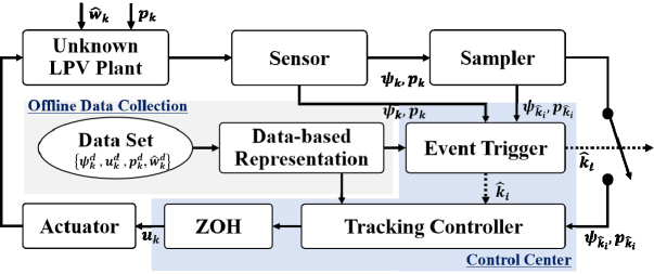
Figure 1: The design schematic of event-triggered LPV control from data.

In what follows, we aim to perform the control synthesis of perturbed LPV systems with closed-loop stability verifications, leading to the data-driven control strategies applicable to both robust stabilization and reference tracking. On the premise of proposed $\theta$-persistence of excitation prerequisite of perturbed LPV systems in Lemma 1, the problems to be addressed in this paper can be briefly summarized by the following keypoints.
Problem 1. For the data-based LPV closed-loop representation with the bounded specification of external perturbations, how to derive the data-based stability certificates and implement the convex programmings feasible at the vertices of the polytopic set of scheduling signal, in purpose of synthesizing data-driven robust stabilization LPV controller.
Problem 2. By deploying the event-triggered communication mechanism, how to incorporate the triggering parameters into data-based stability certificates and develop data-driven event-triggered LPV controller, in terms of the feasibility of convex programming with the finite number of matrix inequalities.
Problem 3. For extending the data-driven event-triggered LPV stabilization control to the scenario of robust tracking, how to construct the integral compensator, leading to augmented LPV systems, and derive the corresponding stability certificates for deploying data-driven event-triggered LPV tracking controller.

3 Learning Event-Triggered LPV Controllers

3.1 Closed-Loop Stability Verification

Recall the specific feedback control strategy $\boldsymbol{u}_{k}\hskip-3.00003pt=\hskip-3.00003ptK_{\hskip-0.81949ptd}(\boldsymbol{p}_{k})\boldsymbol{x}_{k}$ in (13), we further have $\boldsymbol{u}_{k}\hskip-3.00003pt=\hskip-3.00003pt\mathcal{K}\boldsymbol{z}_{k}$ with $\mathcal{K}\hskip-3.00003pt=\hskip-3.00003pt[K_{d0},\bar{K}_{d}]$, where $\bar{K}_{d}\hskip-3.00003pt=\hskip-3.00003pt[K_{d1},\cdots\hskip-1.00006pt,K_{d\ell}]$. Therefore, the closed-loop dynamics of LPV system (4) can be formulated with the form

$$\hskip-6.00006pt\boldsymbol{x}_{k+1}\hskip-3.00003pt \hskip-6.00006pt=\hskip-6.00006pt \hskip-3.00003pt\mathcal{N}\mathrm{Col}(\boldsymbol{z}_{k},\boldsymbol{p}_{k}\hskip-1.99997pt\otimes\hskip-1.99997pt\boldsymbol{p}_{k}\hskip-1.99997pt\otimes\hskip-1.99997pt\boldsymbol{x}_{k})\hskip-1.99997pt+\hskip-1.99997pt\boldsymbol{\omega}_{k},$$ (14)

where $\mathcal{N}\hskip-1.99997pt=\hskip-1.99997pt[A_{d0}\hskip-1.99997pt+\hskip-1.99997ptB_{d0}K_{d0},\bar{A}_{d0}\hskip-1.99997pt+\hskip-1.99997ptB_{d0}\bar{K}_{d}\hskip-1.99997pt+\hskip-1.99997pt\bar{B}_{d}(I_{\ell}\hskip-1.00006pt\otimes\hskip-1.00006ptK_{d0}),\bar{B}_{d}$ $(I_{\ell}\hskip-1.00006pt\otimes\hskip-1.99997pt\bar{K}_{d})]$ with $\hskip-1.00006pt\bar{A}_{d}$ and $\hskip-1.00006pt\bar{B}_{d}$ having the similar structures as $\bar{K}_{d}$. According to the fundamental lemma [17, Lemma 2], we have the data-based closed-loop representation

$$\hskip-6.00006pt\boldsymbol{x}_{k+1}\hskip-3.00003pt \hskip-6.00006pt=\hskip-6.00006pt \hskip-3.00003pt(\boldsymbol{X}_{\hskip-0.81949pt+}\hskip-1.99997pt-\hskip-1.99997pt\boldsymbol{W})\mathcal{V}\mathrm{Col}(\boldsymbol{z}_{k},\boldsymbol{p}_{k}\hskip-1.99997pt\otimes\hskip-1.99997pt\boldsymbol{p}_{k}\hskip-1.99997pt\otimes\hskip-1.99997pt\boldsymbol{x}_{k})\hskip-1.99997pt+\hskip-1.99997pt\boldsymbol{\omega}_{k},$$ (15)

where any $\mathcal{V}\hskip-1.99997pt\in\hskip-1.99997pt\mathds{R}^{\mathcal{T}\times n(1+\ell+\ell^{2})}$ satisfies

$$\mathcal{N}_{cl}\hskip-1.99997pt=\hskip-1.99997pt\left[\hskip-1.99997pt\begin{array}[]{ccc}I_{n}\hskip-1.99997pt&\hskip-1.99997pt\boldsymbol{0}\hskip-1.99997pt&\hskip-1.99997pt\boldsymbol{0}\\ \boldsymbol{0}\hskip-1.99997pt&\hskip-1.99997ptI_{\ell}\otimes I_{n}\hskip-1.99997pt&\hskip-1.99997pt\boldsymbol{0}\\ K_{d0}\hskip-1.99997pt&\hskip-1.99997pt\bar{K}_{d}\hskip-1.99997pt&\hskip-1.99997pt\boldsymbol{0}\\ \boldsymbol{0}\hskip-1.99997pt&\hskip-1.99997ptI_{\ell}\otimes K_{d0}\hskip-1.99997pt&\hskip-1.99997ptI_{\ell}\otimes\bar{K}_{d}\end{array}\hskip-1.99997pt\right]\hskip-3.99994pt=\hskip-1.99997pt\boldsymbol{G}\mathcal{V}$$ (20)

and accordingly $\mathcal{N}\hskip-1.99997pt=\hskip-1.99997pt[\mathcal{A}_{d},\mathcal{B}_{d}]\mathcal{N}_{cl}$. This result leaves the room for designing a data-driven controller that stabilizes all pairs of LPV system (15) for any $\boldsymbol{\omega}_{k}\hskip-3.00003pt\in\hskip-3.00003pt\mathds{B}_{\delta}\hskip-3.00003pt=\hskip-3.00003pt\{\boldsymbol{\omega}|\|\boldsymbol{\omega}\|\hskip-3.00003pt\leq\hskip-3.00003pt\delta\}$.

Theorem 3.2.

For the data matrices generated from $\mathbb{D}_{s}$ in (5), we suppose that there exist the matrix $P\hskip-1.99997pt\in\hskip-1.99997pt\mathbb{S}^{n}_{++}$ and the scalars $\varepsilon_{1}\hskip-1.99997pt\in\hskip-1.99997pt\mathds{R}_{>0}$, $\sigma\hskip-1.99997pt\in\hskip-1.99997pt\mathds{R}_{>1}$ and $\beta_{1}\hskip-1.99997pt\in\hskip-1.99997pt\mathds{R}_{(0,1)}$, such that the condition

$$\left[\hskip-1.99997pt\begin{array}[]{ccccc}\hskip-1.99997ptP\hskip-1.99997pt&\hskip-1.99997pt\boldsymbol{0}\hskip-1.99997pt&\hskip-1.99997ptF^{\top}(\boldsymbol{p}_{k})\boldsymbol{X}^{\top}_{+}\hskip-1.99997pt&\hskip-1.99997ptP\hskip-1.99997pt&\hskip-1.99997ptF^{\top}(\boldsymbol{p}_{k})\hskip-1.99997pt\\ \hskip-1.99997pt\boldsymbol{0}\hskip-1.99997pt&\hskip-1.99997pt\sigma P\hskip-1.99997pt&\hskip-1.99997ptP\hskip-1.99997pt&\hskip-1.99997pt\boldsymbol{0}\hskip-1.99997pt&\hskip-1.99997pt\boldsymbol{0}\hskip-1.99997pt\\ \hskip-1.99997pt\boldsymbol{X}_{+}F(\boldsymbol{p}_{k})\hskip-1.99997pt&\hskip-1.99997ptP\hskip-1.99997pt&\hskip-1.99997ptP-\varepsilon_{1}\Delta\Delta^{\top}\hskip-1.99997pt&\hskip-1.99997pt\boldsymbol{0}\hskip-1.99997pt&\hskip-1.99997pt\boldsymbol{0}\hskip-1.99997pt\\ \hskip-1.99997ptP\hskip-1.99997pt&\hskip-1.99997pt\boldsymbol{0}\hskip-1.99997pt&\hskip-1.99997pt\boldsymbol{0}\hskip-1.99997pt&\hskip-1.99997pt\beta_{1}^{-1}P\hskip-1.99997pt&\hskip-1.99997pt\boldsymbol{0}\hskip-1.99997pt\\ \hskip-1.99997ptF(\boldsymbol{p}_{k})\hskip-1.99997pt&\hskip-1.99997pt\boldsymbol{0}\hskip-1.99997pt&\hskip-1.99997pt\boldsymbol{0}\hskip-1.99997pt&\hskip-1.99997pt\boldsymbol{0}\hskip-1.99997pt&\hskip-1.99997pt\varepsilon_{1}I_{\mathcal{T}}\hskip-1.99997pt\end{array}\hskip-1.99997pt\right]\hskip-3.99994pt\succ\hskip-1.99997pt\boldsymbol{0},$$ (26)

where $F(\boldsymbol{p}_{k})\hskip-1.99997pt=\hskip-1.99997pt\mathcal{V}\mathrm{Col}(I_{n},\boldsymbol{p}_{k}\hskip-1.99997pt\otimes\hskip-1.99997ptI_{n},\boldsymbol{p}_{k}\hskip-1.99997pt\otimes\hskip-1.99997pt\boldsymbol{p}_{k}\hskip-1.99997pt\otimes\hskip-1.99997ptI_{n})P$, holds for the known external perturbation bound $\Delta$. Then, the closed-loop LPV system (14) is exponentially ISS.

Proof 3.3.

By applying Schur complement to (26), we have

$$\hskip-10.00002pt\underbrace{\left[\hskip-1.99997pt\begin{array}[]{cccc}\hskip-1.99997ptP\hskip-1.99997pt&\hskip-1.99997pt\boldsymbol{0}\hskip-1.99997pt&\hskip-1.99997ptF^{\top}(\boldsymbol{p}_{k})\boldsymbol{X}^{\top}_{+}\hskip-1.99997pt&\hskip-1.99997ptP\hskip-1.99997pt\\ \hskip-1.99997pt\boldsymbol{0}\hskip-1.99997pt&\hskip-1.99997pt\sigma P\hskip-1.99997pt&\hskip-1.99997ptP\hskip-1.99997pt&\hskip-1.99997pt\boldsymbol{0}\hskip-1.99997pt\\ \hskip-1.99997pt\boldsymbol{X}_{+}F(\boldsymbol{p}_{k})\hskip-1.99997pt&\hskip-1.99997ptP\hskip-1.99997pt&\hskip-1.99997ptP\hskip-1.99997pt&\hskip-1.99997pt\boldsymbol{0}\hskip-1.99997pt\\ \hskip-1.99997ptP\hskip-1.99997pt&\hskip-1.99997pt\boldsymbol{0}\hskip-1.99997pt&\hskip-1.99997pt\boldsymbol{0}\hskip-1.99997pt&\hskip-1.99997pt\beta_{1}^{-1}P\hskip-1.99997pt\end{array}\hskip-1.99997pt\right]}_{\amalg_{1}}\hskip-1.99997pt-\varepsilon_{1}^{-1}\hskip-3.00003pt\underbrace{\left[\hskip-1.99997pt\begin{array}[]{c}\hskip-1.99997ptF^{\top}\hskip-1.00006pt(\boldsymbol{p}_{k})\hskip-1.99997pt\\ \hskip-1.99997pt\boldsymbol{0}\hskip-1.99997pt\\ \hskip-1.99997pt\boldsymbol{0}\hskip-1.99997pt\\ \hskip-1.99997pt\boldsymbol{0}\hskip-1.99997pt\end{array}\hskip-1.99997pt\right]}_{\bar{F}^{\top}(\boldsymbol{p}_{k})}\hskip-1.99997pt\times$$ (35)

$$\hskip-10.00002pt\bar{F}(\boldsymbol{p}_{k})\hskip-1.99997pt-\hskip-1.99997pt\varepsilon_{1}\mathds{I}_{1}^{\top}\Delta\Delta^{\top}\underbrace{[\boldsymbol{0},\boldsymbol{0},I_{n},\boldsymbol{0}]}_{\mathds{I}_{1}}\hskip-1.99997pt\succ\hskip-1.99997pt\boldsymbol{0}.$$ (36)

Recall the Petersen’s lemma [27], we further obtain

$$\hskip-10.00002pt\amalg_{1}\hskip-1.99997pt-\hskip-1.99997pt\bar{F}^{\hskip-0.81949pt\top}\hskip-1.99997pt(\boldsymbol{p}_{k})\boldsymbol{W}^{\hskip-0.81949pt\top}\hskip-1.99997pt\mathds{I}_{1}\hskip-1.99997pt-\hskip-1.99997pt\mathds{I}_{1}^{\top}\hskip-1.99997pt\boldsymbol{W}\bar{F}(\boldsymbol{p}_{k})\hskip-1.99997pt\succ\hskip-1.99997pt\boldsymbol{0},$$

which is equivalent to

$$\hskip-13.99995pt\left[\hskip-1.99997pt\begin{array}[]{cccc}\hskip-3.00003ptP\hskip-1.99997pt&\hskip-1.99997pt\boldsymbol{0}\hskip-3.00003pt&\hskip-3.00003ptF^{\hskip-0.81949pt\top}\hskip-1.99997pt(\boldsymbol{p}_{k})(\boldsymbol{X}^{\hskip-0.81949pt\top}_{+}\hskip-1.99997pt-\hskip-1.99997pt\boldsymbol{W}^{\top}\hskip-1.99997pt)\hskip-3.00003pt&\hskip-3.00003ptP\hskip-3.00003pt\\ \hskip-3.00003pt\boldsymbol{0}\hskip-1.99997pt&\hskip-1.99997pt\sigma P\hskip-3.00003pt&\hskip-3.00003ptP\hskip-3.00003pt&\hskip-3.00003pt\boldsymbol{0}\hskip-3.00003pt\\ \hskip-3.00003pt(\boldsymbol{X}_{\hskip-0.81949pt+}\hskip-1.99997pt-\hskip-1.99997pt\boldsymbol{W})F(\boldsymbol{p}_{k})\hskip-1.99997pt&\hskip-1.99997ptP\hskip-3.00003pt&\hskip-3.00003ptP\hskip-3.00003pt&\hskip-3.00003pt\boldsymbol{0}\hskip-3.00003pt\\ \hskip-3.00003ptP\hskip-1.99997pt&\hskip-1.99997pt\boldsymbol{0}\hskip-3.00003pt&\hskip-3.00003pt\boldsymbol{0}\hskip-3.00003pt&\hskip-3.00003pt\beta_{1}^{-1}P\hskip-3.00003pt\end{array}\hskip-1.99997pt\right]\hskip-3.00003pt \hskip-8.00003pt\succ\hskip-8.00003pt \boldsymbol{0}.$$ (41)

We then apply Schur complement to (41) and can derive

$$\hskip-10.00002pt\left[\hskip-1.99997pt\begin{array}[]{cc}P\hskip-1.99997pt&\hskip-1.99997pt\boldsymbol{0}\\ \boldsymbol{0}\hskip-1.99997pt&\hskip-1.99997pt\sigma P\end{array}\hskip-1.99997pt\right]\hskip-1.99997pt-\hskip-1.99997pt\left[\hskip-1.99997pt\begin{array}[]{cc}F^{\top}(\boldsymbol{p}_{k})(\boldsymbol{X}_{+}\hskip-1.99997pt-\hskip-1.99997pt\boldsymbol{W})^{\top}\hskip-1.99997pt&\hskip-1.99997ptP\\ P\hskip-1.99997pt&\hskip-1.99997pt\boldsymbol{0}\end{array}\hskip-1.99997pt\right]\hskip-3.00003pt\left[\hskip-1.99997pt\begin{array}[]{cc}P^{-1}\hskip-1.99997pt&\hskip-1.99997pt\boldsymbol{0}\\ \boldsymbol{0}\hskip-1.99997pt&\hskip-1.99997pt\beta_{1}P^{-1}\end{array}\hskip-1.99997pt\right]\hskip-1.99997pt\times$$ (48)

$$\hskip-10.00002pt\left[\hskip-1.99997pt\begin{array}[]{cc}(\boldsymbol{X}_{+}\hskip-1.99997pt-\hskip-1.99997pt\boldsymbol{W})F(\boldsymbol{p}_{k})\hskip-1.99997pt&\hskip-1.99997ptP\\ P\hskip-1.99997pt&\hskip-1.99997pt\boldsymbol{0}\end{array}\hskip-1.99997pt\right]\hskip-1.99997pt\succ\hskip-1.99997pt\boldsymbol{0}.$$ (51)

For performing the theoretical guarantee of exponential ISS of the LPV system (14), we select $V(\boldsymbol{x}_{k})\hskip-1.99997pt=\hskip-1.99997pt\boldsymbol{x}_{k}^{\top}\hskip-1.00006ptP^{-1}\hskip-1.00006pt\boldsymbol{x}_{k}$ as the Lyapunov function, whose forward difference can hence be calculated with the form

$$\hskip-10.00002ptV(\boldsymbol{x}_{k+1})\hskip-1.99997pt-\hskip-1.99997ptV(\boldsymbol{x}_{k}) \hskip-8.00003pt\leq\hskip-8.00003pt -\hskip-1.99997pt\beta_{1}V(\boldsymbol{x}_{k})\hskip-1.99997pt+\hskip-1.99997pt\sigma\boldsymbol{\omega}_{k}^{\top}P^{-1}\boldsymbol{\omega_{k}}.$$ (52)

In view of the congruence transformation of (51) by pre- and post-multiplying its both sides with $\mathrm{Blkdiag}(P^{-1}\hskip-1.00006pt,\hskip-1.00006ptP^{-1}\hskip-1.00006pt)$, the equivalence between (51) and (52) can be well established. In addition, (52) further yields

$$\hskip-10.00002ptV(\boldsymbol{x}_{k+1})\hskip-1.99997pt-\hskip-1.99997ptV(\boldsymbol{x}_{k}) \hskip-8.00003pt\leq\hskip-8.00003pt -\hskip-1.99997pt\beta_{1}V(\boldsymbol{x}_{k})\hskip-1.99997pt+\hskip-1.99997pt\sigma\mu_{\max}(P^{-1})\|\omega_{k}\|^{2}$$ (53)

$$\hskip-8.00003pt=\hskip-8.00003pt -\hskip-1.99997pt\beta_{1}V(\boldsymbol{x}_{k})+\hbar(\|\omega_{k}\|).$$

Obviously, $\hbar(\|\omega_{k}\|)$ implies the $\mathcal{K}$-function with respect to the variable $\|\omega_{k}\|$. By performing the recursive calculations about (53), we can derive

$$\hskip-10.00002ptV(\boldsymbol{x}_{k}) \hskip-8.00003pt\leq\hskip-8.00003pt (1\hskip-1.99997pt-\hskip-1.99997pt\beta_{1})^{k}V(\boldsymbol{x}_{0})\hskip-1.99997pt+\hskip-1.99997pt\sum\nolimits_{i=0}^{k-1}\hskip-1.99997pt(1\hskip-1.99997pt-\hskip-1.99997pt\beta_{1})^{k-1-i}\hbar(\|\omega_{i}\|),$$

which leads to

$$\hskip-10.00002pt\|\boldsymbol{x}_{k}\| \hskip-8.00003pt\leq\hskip-8.00003pt e^{-\beta_{1}k/2}\mathcal{R}\|\boldsymbol{x}_{0}\|+\gamma_{1}(\|\boldsymbol{\omega_{s}}\|_{[0,k-1]}),$$ (54)

with $\mathcal{R}\hskip-1.99997pt=\hskip-1.99997pt\lambda_{\max}^{1/2}(\hskip-1.00006ptP^{-1}\hskip-1.00006pt)/\lambda_{\min}^{1/2}(\hskip-1.00006ptP^{-1}\hskip-1.00006pt)$ implying the overshoot and

$$\hskip-10.00002pt\gamma_{1}(\|\boldsymbol{\omega_{s}}\|_{[0,k-1]}) \hskip-8.99994pt=\hskip-8.99994pt c_{1}\hskip-1.99997pt\sum\nolimits_{i=1}^{k-1}\hskip-1.99997pte^{-\beta_{1}(k-1-i)/2}\hbar(\|\boldsymbol{\omega_{s}}\|_{[0,k-1]}),$$

holding with $c_{1}\hskip-1.99997pt=\hskip-1.99997pt\lambda_{\min}^{-1/2}(\hskip-1.00006ptP^{-1}\hskip-1.00006pt)$. Therefore, the exponential ISS of the closed-loop LPV system (14) is ensured, which completes the proof.

3.2 Data-Based Control Synthesis

Note that the term $F(\boldsymbol{p}_{k})$ in (26) is quadratically dependent on $\boldsymbol{p}_{k}$, which implies the intrinsical difficulty on reducing (26) to a finite number of constraints solved by convex optimization toolkits. In this subsection, we consider $\mathds{P}$ as a polytope, such that the convex relaxations can be defined by its vertices with the aid of full-block $\mathrm{S}$-procedure [48]. Within this context, we define two matrices $\hskip-1.00006pt\mathcal{F}\hskip-3.00003pt\in\hskip-3.00003pt\mathds{R}^{\mathcal{T}\hskip-0.81949pt\times\hskip-0.81949ptn(1\hskip-0.81949pt+\hskip-0.81949pt\ell\hskip-0.81949pt+\hskip-0.81949pt\ell^{2})}\hskip-1.99997pt$ and $\hskip-1.00006ptF_{Q}\hskip-3.00003pt\in\hskip-3.00003pt\mathds{R}^{\mathcal{T}(1\hskip-0.81949pt+\hskip-0.81949pt\ell)\hskip-0.81949pt\times\hskip-0.81949ptn(1+\ell)}\hskip-1.00006pt$, such that $F(\boldsymbol{p}_{k})$ can be rewritten with the form

$$\hskip-6.00006ptF(\boldsymbol{p}_{k})\hskip-1.99997pt=\hskip-1.99997pt\mathcal{F}\hskip-1.99997pt\left[\hskip-1.99997pt\begin{array}[]{c}\hskip-1.99997ptI_{n}\hskip-1.99997pt\\ \hskip-1.99997pt\boldsymbol{p}_{k}\hskip-1.99997pt\otimes\hskip-1.99997ptI_{n}\hskip-1.99997pt\\ \hskip-1.99997pt\boldsymbol{p}_{k}\hskip-1.99997pt\otimes\hskip-1.99997pt\boldsymbol{p}_{k}\hskip-1.99997pt\otimes\hskip-1.99997ptI_{n}\hskip-1.99997pt\end{array}\hskip-1.99997pt\right]\hskip-3.00003pt=\hskip-3.00003pt\left[\hskip-1.99997pt\begin{array}[]{c}\hskip-1.99997ptI_{\mathcal{T}}\hskip-1.99997pt\\ \hskip-1.99997pt\boldsymbol{p}_{k}\hskip-1.99997pt\otimes\hskip-1.99997ptI_{\mathcal{T}}\hskip-1.99997pt\end{array}\hskip-1.99997pt\right]^{\hskip-0.81949pt\top}\hskip-3.00003ptF_{Q}\hskip-1.99997pt\left[\hskip-1.99997pt\begin{array}[]{c}\hskip-1.99997ptI_{n}\hskip-1.99997pt\\ \hskip-1.99997pt\boldsymbol{p}_{k}\hskip-1.99997pt\otimes\hskip-1.99997ptI_{n}\hskip-1.99997pt\end{array}\hskip-1.99997pt\right],$$ (62)

based on which, we can further lead to the controller synthesis with strict stability guarantee by the following theorem.

Theorem 3.4.

For the data matrices generated from $\mathbb{D}_{s}$ in (5), we suppose that there exist the matrices $P\hskip-1.99997pt\in\hskip-1.99997pt\mathbb{S}^{n}_{++}$, $Z_{0}\hskip-1.99997pt\in\hskip-1.99997pt\mathds{R}^{m\times n}$, $\bar{Z}\hskip-1.99997pt\in\hskip-1.99997pt\mathds{R}^{m\times\ell n}$, and $\Xi\hskip-1.99997pt\in\hskip-1.99997pt\mathbb{S}^{2\ell(4n+\mathcal{T})}$, such that

$$\hskip-6.00006pt\mathcal{N}_{cl}\left[\hskip-1.99997pt\begin{array}[]{ccc}\hskip-1.99997ptP\hskip-1.99997pt&\hskip-1.99997pt\boldsymbol{0}\hskip-1.99997pt&\hskip-1.99997pt\boldsymbol{0}\hskip-1.99997pt\\ \hskip-1.99997pt\boldsymbol{0}\hskip-1.99997pt&\hskip-1.99997ptI_{\ell}\hskip-1.99997pt\otimes\hskip-1.99997ptP\hskip-1.99997pt&\hskip-1.99997pt\boldsymbol{0}\hskip-1.99997pt\\ \hskip-1.99997pt\boldsymbol{0}\hskip-1.99997pt&\hskip-1.99997pt\boldsymbol{0}\hskip-1.99997pt&\hskip-1.99997ptI_{\ell}\hskip-1.99997pt\otimes\hskip-1.99997ptP\hskip-1.99997pt\otimes\hskip-1.99997ptP\hskip-1.99997pt\end{array}\hskip-1.99997pt\right]\hskip-1.99997pt=\hskip-1.99997pt\boldsymbol{G}\mathcal{F},$$ (66)

and the following conditions

$$\hskip-6.00006pt\left[\hskip-1.99997pt\begin{array}[]{cc}\hskip-1.99997ptM_{11}\hskip-1.99997pt&\hskip-1.99997ptM_{12}\hskip-1.99997pt\\ \hskip-1.99997ptI\hskip-1.99997pt&\hskip-1.99997pt\boldsymbol{0}\hskip-1.99997pt\\ \hskip-1.99997ptM_{21}\hskip-1.99997pt&\hskip-1.99997ptM_{22}\hskip-1.99997pt\end{array}\hskip-1.99997pt\right]^{\hskip-1.63885pt\top}\hskip-3.00003pt\left[\hskip-1.99997pt\begin{array}[]{cc}\hskip-1.99997pt\Xi\hskip-1.99997pt&\hskip-1.99997pt\boldsymbol{0}\hskip-1.99997pt\\ \hskip-1.99997pt\boldsymbol{0}\hskip-1.99997pt&\hskip-1.99997pt-\Phi\hskip-1.99997pt\end{array}\hskip-1.99997pt\right]\hskip-1.99997pt\left[\hskip-1.99997pt\begin{array}[]{cc}\hskip-1.99997ptM_{11}\hskip-1.99997pt&\hskip-1.99997ptM_{12}\hskip-1.99997pt\\ \hskip-1.99997ptI\hskip-1.99997pt&\hskip-1.99997pt\boldsymbol{0}\hskip-1.99997pt\\ \hskip-1.99997ptM_{21}\hskip-1.99997pt&\hskip-1.99997ptM_{22}\hskip-1.99997pt\end{array}\hskip-1.99997pt\right] \hskip-3.00003pt\prec\hskip-1.99997pt\boldsymbol{0},$$ (67i)

$$\hskip-6.00006pt\left[\hskip-1.99997pt\begin{array}[]{c}\hskip-1.99997ptI\hskip-1.99997pt\\ \hskip-1.99997pt\Upsilon(\boldsymbol{p}_{k})\hskip-1.99997pt\end{array}\hskip-1.99997pt\right]^{\hskip-1.63885pt\top}\hskip-1.99997pt\left[\hskip-1.99997pt\begin{array}[]{cc}\hskip-1.99997pt\Xi_{11}\hskip-1.99997pt&\hskip-1.99997pt\Xi_{12}\hskip-1.99997pt\\ \hskip-1.99997pt\Xi_{12}^{\top}\hskip-1.99997pt&\hskip-1.99997pt\Xi_{22}\hskip-1.99997pt\end{array}\hskip-1.99997pt\right]\hskip-1.99997pt\left[\hskip-1.99997pt\begin{array}[]{c}\hskip-1.99997ptI\hskip-1.99997pt\\ \hskip-1.99997pt\Upsilon(\boldsymbol{p}_{k})\hskip-1.99997pt\end{array}\hskip-1.99997pt\right] \hskip-3.00003pt\succeq\hskip-1.99997pt\boldsymbol{0},$$ (67p)

$$\hskip-6.00006pt\Xi_{22} \hskip-3.00003pt\prec\hskip-1.99997pt\boldsymbol{0},$$ (67q)

$$\hskip-6.00006pt\left[\hskip-1.99997pt\begin{array}[]{ccc}\hskip-1.99997ptP\hskip-1.99997pt&\hskip-1.99997pt\boldsymbol{0}\hskip-1.99997pt&\hskip-1.99997pt\boldsymbol{0}\hskip-1.99997pt\\ \hskip-1.99997pt\boldsymbol{0}\hskip-1.99997pt&\hskip-1.99997ptI_{\ell}\hskip-1.99997pt\otimes\hskip-1.99997ptP\hskip-1.99997pt&\hskip-1.99997pt\boldsymbol{0}\hskip-1.99997pt\\ \hskip-1.99997ptZ_{0}\hskip-1.99997pt&\hskip-1.99997pt\bar{Z}\hskip-1.99997pt&\hskip-1.99997pt\boldsymbol{0}\hskip-1.99997pt\\ \hskip-1.99997pt\boldsymbol{0}\hskip-1.99997pt&\hskip-1.99997ptI_{\ell}\hskip-1.99997pt\otimes\hskip-1.99997ptZ_{0}\hskip-1.99997pt&\hskip-1.99997ptI_{\ell}\hskip-1.99997pt\otimes\hskip-1.99997pt\bar{Z}\hskip-1.99997pt\end{array}\hskip-1.99997pt\right] \hskip-3.00003pt=\hskip-1.99997pt\boldsymbol{G}\mathcal{F},$$ (67v)

holding for all $\boldsymbol{p}_{k}\hskip-1.99997pt\in\hskip-1.99997pt\mathbb{P}$, where

$$\hskip-6.00006pt\Upsilon(\boldsymbol{p}_{k})\hskip-1.99997pt= \mathrm{Blkdiag}(\mathrm{Diag}(\boldsymbol{p}_{k}\hskip-1.99997pt\otimes\hskip-1.99997ptI_{n}),\mathrm{Diag}(\boldsymbol{p}_{k}\hskip-1.99997pt\otimes\hskip-1.99997ptI_{n}),$$

$$\mathrm{Diag}(\boldsymbol{p}_{k}\hskip-1.99997pt\otimes\hskip-1.99997ptI_{n}),\mathrm{Diag}(\boldsymbol{p}_{k}\hskip-1.99997pt\otimes\hskip-1.99997ptI_{n}),\mathrm{Diag}(\boldsymbol{p}_{k}\hskip-1.99997pt\otimes\hskip-1.99997ptI_{\mathcal{T}})),$$ (68a)

$$\hskip-6.00006ptM_{11}\hskip-1.99997pt= \boldsymbol{0}_{\ell(4n+\mathcal{T})\times\ell(4n+\mathcal{T})},$$ (68b)

$$\hskip-6.00006ptM_{12}\hskip-1.99997pt= \mathrm{Blkdiag}(\boldsymbol{1}_{\ell}\hskip-3.00003pt\otimes\hskip-1.99997ptI_{n},\hskip-1.00006pt\boldsymbol{1}_{\ell}\hskip-3.00003pt\otimes\hskip-1.99997ptI_{n},\hskip-1.00006pt\boldsymbol{1}_{\ell}\hskip-3.00003pt\otimes\hskip-1.99997ptI_{n},\hskip-1.00006pt\boldsymbol{1}_{\ell}\hskip-3.00003pt\otimes\hskip-1.99997ptI_{n},\hskip-1.00006pt\boldsymbol{1}_{\ell}\hskip-3.00003pt\otimes\hskip-1.99997ptI_{\mathcal{T}}\hskip-1.00006pt),$$ (68c)

$$\hskip-6.00006ptM_{21}\hskip-1.99997pt= \mathrm{Blkdiag}\left(\left[\hskip-1.99997pt\begin{array}[]{c}\hskip-1.99997pt\boldsymbol{0}_{n\times\ell n}\hskip-1.99997pt\\ \hskip-1.99997ptI_{\ell n}\hskip-1.99997pt\end{array}\hskip-1.99997pt\right],\left[\hskip-1.99997pt\begin{array}[]{c}\hskip-1.99997pt\boldsymbol{0}_{n\times\ell n}\hskip-1.99997pt\\ \hskip-1.99997ptI_{\ell n}\hskip-1.99997pt\end{array}\hskip-1.99997pt\right],\left[\hskip-1.99997pt\begin{array}[]{c}\hskip-1.99997pt\boldsymbol{0}_{n\times\ell n}\hskip-1.99997pt\\ \hskip-1.99997ptI_{\ell n}\hskip-1.99997pt\end{array}\hskip-1.99997pt\right],\right.$$ (68j)

$$\left.\left[\hskip-1.99997pt\begin{array}[]{c}\hskip-1.99997pt\boldsymbol{0}_{n\times\ell n}\hskip-1.99997pt\\ \hskip-1.99997ptI_{\ell n}\hskip-1.99997pt\end{array}\hskip-1.99997pt\right],\left[\hskip-1.99997pt\begin{array}[]{c}\hskip-1.99997pt\boldsymbol{0}_{\mathcal{T}\times\ell\mathcal{T}}\hskip-1.99997pt\\ \hskip-1.99997ptI_{\ell\mathcal{T}}\hskip-1.99997pt\end{array}\hskip-1.99997pt\right]\right),$$ (68o)

$$\hskip-6.00006ptM_{22}\hskip-1.99997pt= \mathrm{Blkdiag}\left(\left[\hskip-1.99997pt\begin{array}[]{c}\hskip-1.99997ptI_{n}\hskip-1.99997pt\\ \hskip-1.99997pt\boldsymbol{0}_{\ell n\times n}\hskip-1.99997pt\end{array}\hskip-1.99997pt\right],\left[\hskip-1.99997pt\begin{array}[]{c}\hskip-1.99997ptI_{n}\hskip-1.99997pt\\ \hskip-1.99997pt\boldsymbol{0}_{\ell n\times n}\hskip-1.99997pt\end{array}\hskip-1.99997pt\right],\left[\hskip-1.99997pt\begin{array}[]{c}\hskip-1.99997ptI_{n}\hskip-1.99997pt\\ \hskip-1.99997pt\boldsymbol{0}_{\ell n\times n}\hskip-1.99997pt\end{array}\hskip-1.99997pt\right],\right.$$ (68v)

$$\left.\left[\hskip-1.99997pt\begin{array}[]{c}\hskip-1.99997ptI_{n}\hskip-1.99997pt\\ \hskip-1.99997pt\boldsymbol{0}_{\ell n\times n}\hskip-1.99997pt\end{array}\hskip-1.99997pt\right],\left[\hskip-1.99997pt\begin{array}[]{c}\hskip-1.99997ptI_{\mathcal{T}}\hskip-1.99997pt\\ \hskip-1.99997pt\boldsymbol{0}_{\ell\mathcal{T}\times\mathcal{T}}\hskip-1.99997pt\end{array}\hskip-1.99997pt\right]\right),$$ (68aa)

$$\hskip-6.00006pt\Phi\hskip-1.99997pt= \left[\hskip-1.99997pt\begin{array}[]{ccccc}\hskip-1.99997pt\mathcal{Y}\hskip-1.99997pt&\hskip-1.99997pt\boldsymbol{0}\hskip-1.99997pt&\hskip-1.99997pt(\mathcal{X}_{+}F_{Q})^{\top}\hskip-1.99997pt&\hskip-1.99997pt\mathcal{Y}\hskip-1.99997pt&\hskip-1.99997ptF^{\top}_{Q}\hskip-1.99997pt\\ \hskip-1.99997pt\boldsymbol{0}\hskip-1.99997pt&\hskip-1.99997pt\sigma\mathcal{Y}\hskip-1.99997pt&\hskip-1.99997pt\mathcal{Y}\hskip-1.99997pt&\hskip-1.99997pt\boldsymbol{0}\hskip-1.99997pt&\hskip-1.99997pt\boldsymbol{0}\hskip-1.99997pt\\ \hskip-1.99997pt\mathcal{X}_{+}F_{Q}\hskip-1.99997pt&\hskip-1.99997pt\mathcal{Y}\hskip-1.99997pt&\hskip-1.99997pt\bar{\mathcal{Y}}\hskip-1.99997pt&\hskip-1.99997pt\boldsymbol{0}\hskip-1.99997pt&\hskip-1.99997pt\boldsymbol{0}\hskip-1.99997pt\\ \hskip-1.99997pt\mathcal{Y}\hskip-1.99997pt&\hskip-1.99997pt\boldsymbol{0}\hskip-1.99997pt&\hskip-1.99997pt\boldsymbol{0}\hskip-1.99997pt&\hskip-1.99997pt\beta_{1}^{-1}\mathcal{Y}\hskip-1.99997pt&\hskip-1.99997pt\boldsymbol{0}\hskip-1.99997pt\\ \hskip-1.99997ptF_{Q}\hskip-1.99997pt&\hskip-1.99997pt\boldsymbol{0}\hskip-1.99997pt&\hskip-1.99997pt\boldsymbol{0}\hskip-1.99997pt&\hskip-1.99997pt\boldsymbol{0}\hskip-1.99997pt&\hskip-1.99997pt\mathcal{E}\hskip-1.99997pt\end{array}\hskip-1.99997pt\right],$$ (68ag)

with $\boldsymbol{1}_{n}\hskip-1.99997pt=\hskip-1.99997pt\mathrm{Col}(1,\cdots,1)\hskip-1.99997pt\in\hskip-1.99997pt\mathds{R}^{n}$ and

$$\hskip-6.00006pt\mathcal{Y}\hskip-1.99997pt= \mathrm{Blkdiag}(P,\boldsymbol{0}_{\ell n\times\ell n}),$$

$$\hskip-6.00006pt\bar{\mathcal{Y}}\hskip-1.99997pt= \mathrm{Blkdiag}(P\hskip-1.99997pt-\hskip-1.99997pt\varepsilon_{1}\Delta\Delta^{\top},\boldsymbol{0}_{\ell n\times\ell n}),$$

$$\hskip-6.00006pt\mathcal{E}\hskip-1.99997pt= \mathrm{Blkdiag}(\varepsilon_{1}I_{\mathcal{T}},\boldsymbol{0}_{\ell\mathcal{T}\times\ell\mathcal{T}}),$$

$$\hskip-6.00006pt\mathcal{X}_{+}\hskip-1.99997pt= \mathrm{Blkdiag}(\boldsymbol{X}_{+},I_{\ell}\otimes\boldsymbol{X}_{+}).$$

Then, the state-feedback controller $\boldsymbol{u}_{k}\hskip-3.00003pt=\hskip-3.00003ptK_{\hskip-0.81949ptd}(\boldsymbol{p}_{k})\boldsymbol{x}_{k}$ as (13) can be constructed by

$$K_{d0}\hskip-1.99997pt=\hskip-1.99997ptZ_{0}P^{-1},\bar{K}_{d}\hskip-1.99997pt=\hskip-1.99997pt\bar{Z}(I_{\ell}\otimes P)^{-1},$$ (70)

which ensures the exponential ISS of closed-loop system (14).

Proof 3.5.

We recall the definition of $F_{Q}$ in (62) and utilize the Kronecker property, refer to [42, Eq.(1)], twice times with regard to the term $\boldsymbol{X}_{+}F(\boldsymbol{p}_{k})$, which leads to

$$\hskip-6.00006pt\boldsymbol{X}_{+}F(\boldsymbol{p}_{k})\hskip-1.99997pt=\hskip-1.99997pt\hskip-1.99997pt\left[\hskip-1.99997pt\begin{array}[]{c}\hskip-1.99997ptI_{n}\hskip-1.99997pt\\ \hskip-1.99997pt\boldsymbol{p}_{k}\hskip-1.99997pt\otimes\hskip-1.99997ptI_{n}\hskip-1.99997pt\end{array}\hskip-1.99997pt\right]^{\hskip-0.81949pt\top}\hskip-1.99997pt\mathcal{X}_{+}F_{Q}\left[\hskip-1.99997pt\begin{array}[]{c}\hskip-1.99997ptI_{n}\hskip-1.99997pt\\ \hskip-1.99997pt\boldsymbol{p}_{k}\hskip-1.99997pt\otimes\hskip-1.99997ptI_{n}\hskip-1.99997pt\end{array}\hskip-1.99997pt\right].$$ (75)

By combining (26) with (75), we then obtain that

$$\hskip-6.00006ptM^{\top}(\boldsymbol{p}_{k})\Phi M(\boldsymbol{p}_{k})\hskip-1.99997pt\succ\hskip-1.99997pt\boldsymbol{0},$$ (76)

is satisfied with $\Psi$ defined in (68ag) and $M(\boldsymbol{p}_{k})$ formulated by

$$\hskip-6.00006ptM(\boldsymbol{p}_{k})\hskip-1.99997pt=\hskip-1.99997ptM_{22}\hskip-1.99997pt+\hskip-1.99997ptM_{21}\hskip-1.99997pt\Upsilon(\boldsymbol{p}_{k})(I\hskip-1.99997pt-\hskip-1.99997ptM_{11}\hskip-1.99997pt\Upsilon(\boldsymbol{p}_{k}))^{-1}\hskip-1.99997ptM_{12},$$ (77)

where $M_{ij}$ with $i,j\hskip-1.99997pt\in\hskip-1.99997pt\mathds{N}_{[1,2]}$ can be represented by (68b)-(68aa), respectively. By virtue of utilizing the full-block S-procedure [48, Theorem 8] and supposing $\Xi_{22}\hskip-1.99997pt\prec\hskip-1.99997pt\mathbf{0}$, the inequality (67p) is no longer multi-convexity about $\boldsymbol{p}_{k}$, such that a finite set of matrix inequalities can be specifically satisfied at the vertices $\hat{\boldsymbol{p}}_{k}^{i}$ of polytopic scheduling signal set $\mathbb{P}$, that is

$$\hskip-6.00006pt\left[\hskip-1.99997pt\begin{array}[]{c}\hskip-1.99997ptI\hskip-1.99997pt\\ \hskip-1.99997pt\Upsilon(\hat{\boldsymbol{p}}_{k}^{i})\hskip-1.99997pt\end{array}\hskip-1.99997pt\right]^{\hskip-1.63885pt\top}\hskip-1.99997pt\left[\hskip-1.99997pt\begin{array}[]{cc}\hskip-1.99997pt\Xi_{11}\hskip-1.99997pt&\hskip-1.99997pt\Xi_{12}\hskip-1.99997pt\\ \hskip-1.99997pt\Xi_{12}^{\top}\hskip-1.99997pt&\hskip-1.99997pt\Xi_{22}\hskip-1.99997pt\end{array}\hskip-1.99997pt\right]\hskip-1.99997pt\left[\hskip-1.99997pt\begin{array}[]{c}\hskip-1.99997ptI\hskip-1.99997pt\\ \hskip-1.99997pt\Upsilon(\hat{\boldsymbol{p}}_{k}^{i})\hskip-1.99997pt\end{array}\hskip-1.99997pt\right] \hskip-3.00003pt\succeq\hskip-1.99997pt\boldsymbol{0},i\in\mathds{N}_{[1,n]}.$$ (84)

Besides, substituting (20) into (66) yields

$$\hskip-6.00006pt\left[\hskip-1.99997pt\begin{array}[]{ccc}\hskip-1.99997ptP\hskip-1.99997pt&\hskip-1.99997pt\boldsymbol{0}\hskip-1.99997pt&\hskip-1.99997pt\boldsymbol{0}\hskip-1.99997pt\\ \hskip-1.99997pt\boldsymbol{0}\hskip-1.99997pt&\hskip-1.99997ptI_{\ell}\hskip-1.99997pt\otimes\hskip-1.99997ptP\hskip-1.99997pt&\hskip-1.99997pt\boldsymbol{0}\hskip-1.99997pt\\ \hskip-1.99997ptK_{d0}\hskip-1.99997pt&\hskip-1.99997pt\bar{K}_{d}(I_{\ell}\otimes P)\hskip-1.99997pt&\hskip-1.99997pt\boldsymbol{0}\hskip-1.99997pt\\ \hskip-1.99997pt\boldsymbol{0}\hskip-1.99997pt&\hskip-1.99997ptI_{\ell}\otimes K_{d0}\hskip-1.99997pt&\hskip-1.99997ptI_{\ell}\otimes\bar{K}_{d}(I_{\ell}\otimes P)\hskip-1.99997pt\end{array}\hskip-1.99997pt\right]\hskip-1.99997pt=\hskip-1.99997pt\boldsymbol{G}\mathcal{F}.$$ (89)

We let $Z_{0}\hskip-1.99997pt=\hskip-1.99997ptK_{0}P$ and $\bar{Z}\hskip-1.99997pt=\hskip-1.99997pt\bar{K}_{d}(I_{\ell}\hskip-1.99997pt\otimes\hskip-1.99997ptP)$, hence (67v) holds. Note that if there exist $Z_{0}$ and $\bar{Z}$ satisfying (67v), then the control synthesis with the form (70) provides the $\mathcal{N}_{cl}$ satisfying (66). Up till now, we complete the proof of this theorem.

Remark 3.6.

In order to cope with the dependency of $F(\boldsymbol{p}_{k})$ on $\boldsymbol{p}_{k}$, we express the matrix inequality (26) with an equivalent data-dependent form (67i)-(67q), in the light of full-block S-procedure [44, Section IV], such that the decision variables $P$ and $F_{Q}$ can be calculated via a finite number of inequality constraints at the vertices of polytopic scheduling signal set $\mathds{P}$. Therefore, the controller gains can be scheduled, once the constraint (67v) is satisfied. Our theoretical results correspond to perturbed LPV systems, where the perturbations stem from unmodeled dynamics or external disturbance. Compared to the existing work [42], although we do not view the perturbations as the process noises, the technical content can be potentially extended to the scenario that considers the measurement noises during data collection, leading to $\hat{\boldsymbol{x}}\hskip-1.99997pt=\hskip-1.99997pt\boldsymbol{x}\hskip-1.99997pt+\hskip-1.99997pt\hat{\boldsymbol{d}}$ with $\hat{\boldsymbol{d}}$ representing the noise signal, such that the above theorems can be combined with [27, Remark 3] to address this issue.

3.3 Event-Triggered Communication Scheme

Apart from ensuring the closed-loop stability of LPV system, we aim to refine the communication efficiency while developing robust controller from available data directly in the sense of networked control. The sequence of transmission instants is denoted by $\{\hat{k}_{i}\},i\hskip-1.99997pt\in\hskip-1.99997pt\mathds{N}$. Allowing for the zero-order-hold (ZOH), the control input can be depicted by

$$\boldsymbol{u}_{k}\hskip-1.99997pt=\hskip-1.99997ptK_{d}(\boldsymbol{p}_{\hat{k}_{i}})\boldsymbol{x}_{\hat{k}_{i}},k\hskip-1.99997pt\in\hskip-1.99997pt\mathds{N}_{[\hat{k}_{i},\hat{k}_{i+1})},$$ (90)

based on which, the closed-loop LPV system can then be described by

$$\hskip-6.00006pt\boldsymbol{x}_{k+1}\hskip-3.00003pt \hskip-6.00006pt=\hskip-6.00006pt \hskip-3.00003ptA_{d}(\boldsymbol{p}_{k})\boldsymbol{x}_{k}\hskip-1.99997pt+\hskip-1.99997ptB_{d}(\boldsymbol{p}_{k})\boldsymbol{u}_{\hat{k}_{i}}\hskip-1.99997pt+\hskip-1.99997pt\boldsymbol{\omega_{k}},$$ (91)

$$\hskip-6.00006pt=\hskip-6.00006pt \hskip-3.00003pt(A_{d}(\boldsymbol{p}_{k})+B_{d}K_{d}(\boldsymbol{p}_{k}))\boldsymbol{x}_{k}\hskip-1.99997pt+\hskip-1.99997pt\boldsymbol{\nu}_{k}\hskip-1.99997pt+\hskip-1.99997pt\boldsymbol{\omega}_{k},$$

where $\boldsymbol{\nu}_{k}$ is with the form

$$\hskip-6.00006pt\boldsymbol{\nu}_{k}\hskip-3.00003pt \hskip-6.00006pt=\hskip-6.00006pt \hskip-3.00003ptB_{d}(\boldsymbol{p}_{k})K_{d}(\boldsymbol{p}_{k})\boldsymbol{e}(k)+$$ (92)

$$\hskip-3.00003ptB_{d}(\boldsymbol{p}_{k})(K_{d}(\boldsymbol{p}_{\hat{k}_{i}})-K_{d}(\boldsymbol{p}_{k}))\boldsymbol{x}_{\hat{k}_{i}},$$

in which $\boldsymbol{e}_{k}\hskip-1.99997pt=\hskip-1.99997pt\boldsymbol{x}_{\hat{k}_{i}}\hskip-1.99997pt-\hskip-1.99997pt\boldsymbol{x}_{k}$ represents the sampling-induced error capturing the discrepancy between the recently transmitted and the current sampled system states. Accordingly, we can rewrite the LPV system (91) with the data-based form

$$\hskip-6.00006pt\boldsymbol{x}_{k+1}\hskip-3.00003pt \hskip-6.00006pt=\hskip-6.00006pt \hskip-3.00003pt(\boldsymbol{X}_{\hskip-0.81949pt+}\hskip-1.99997pt-\hskip-1.99997pt\boldsymbol{W})\mathcal{V}\mathrm{Col}(\boldsymbol{z}_{k},\boldsymbol{p}_{k}\hskip-1.99997pt\otimes\hskip-1.99997pt\boldsymbol{p}_{k}\hskip-1.99997pt\otimes\hskip-1.99997pt\boldsymbol{x}_{k})\hskip-1.99997pt+\hskip-1.99997pt\boldsymbol{\nu}_{k}\hskip-1.99997pt+\hskip-1.99997pt\boldsymbol{\omega}_{k}.$$ (93)

Remark 3.7.

Note that $\boldsymbol{\nu}_{k}$ embedded in the data-based representation of LPV system (93) indirectly depends on the data matrices. Compared with the event-triggered linear time-invariant systems [37, 47], $\boldsymbol{\nu}_{k}$ consists of not only the sampling-induced error $\boldsymbol{e}_{k}$ but also the scheduling variable $\boldsymbol{p}_{k}$. For the sake of convenience, we treat $\boldsymbol{\nu}_{k}$ as a whole and use it to develop the event-triggered logic in this paper. Albeit the matrix $B_{d}(\boldsymbol{p}_{k})$ in (92) is unknown for control design, we can leverage the data-based representation $[\mathcal{A}_{d},\mathcal{B}_{d}]\hskip-1.99997pt=\hskip-1.99997pt(\hskip-1.00006pt\boldsymbol{X}_{\hskip-1.63885pt+}\hskip-1.99997pt-\hskip-1.99997pt\boldsymbol{W})\boldsymbol{G}^{+}\hskip-1.00006pt$ and obtain that $\mathcal{B}_{d}$ can be extracted from the $n(1\hskip-1.99997pt+\hskip-1.99997pt\ell)\hskip-1.99997pt+\hskip-1.99997pt1$-th to the $(m\hskip-1.99997pt+\hskip-1.99997ptn)(1\hskip-1.99997pt+\hskip-1.99997pt\ell)$-th column of $(\boldsymbol{X}_{\hskip-0.81949pt+}\hskip-1.99997pt-\hskip-1.99997pt\boldsymbol{W})\boldsymbol{G}^{+}\hskip-1.00006pt$. Motivated by [37], the resulting control gains (70) can be potentially utilized to determine the triggering parameters in what follows. Hence, the signal $\hskip-1.00006pt\boldsymbol{\nu}_{k}$ is available for the event detector to confirm the networked communication transmissions.

We recall the sequence of triggering instants $\hskip-1.00006pt\{\hat{k}_{i}\},i\hskip-1.99997pt\in\hskip-1.99997pt\mathds{N}\hskip-1.00006pt$ with $\hat{k}_{0}\hskip-1.99997pt=\hskip-1.99997pt0$, then the triggering logic can be specified with the form

$$\hskip-6.00006pt\hat{k}_{i+1}\hskip-3.00003pt \hskip-6.00006pt=\hskip-6.00006pt \hskip-3.00003pt\inf\left\{k>\hat{k}_{i}|\boldsymbol{\nu}^{\top}_{k}\Psi_{1}\boldsymbol{\nu}_{k}\geq\boldsymbol{x}_{k}^{\top}\Psi_{2}\boldsymbol{x}_{k}+v\right\},$$ (94)

where $\hskip-1.00006ptv\hskip-1.99997pt\in\hskip-1.99997pt\mathds{R}_{>0}\hskip-1.00006pt$ implies an arbitrary constant, and $\hskip-1.00006pt\Psi_{1}\hskip-1.00006pt$ and $\hskip-1.00006pt\Psi_{2}$ are positively definite matrices to be determined later.

Theorem 3.8.

For the event-triggered LPV system (93) together with the data set $\mathbb{D}_{s}$, we suppose that Lemma 1 and (67) hold, leading to the feasible solution (70), thus (93) is practically exponentially ISS, if there exist $\mu,\varepsilon_{2}\in\mathds{R}_{+}$ and $\Psi_{1},\Psi_{2}\hskip-1.99997pt\in\hskip-1.99997pt\mathbb{S}_{++}^{n}$, such that

$$\hskip-13.99995pt\left[\hskip-1.99997pt\begin{array}[]{ccc}\hskip-3.00003pt\Omega_{11}\hskip-1.99997pt&\hskip-1.99997pt\Omega_{12}\hskip-3.00003pt&\hskip-3.00003pt\Omega_{13}\\ \hskip-3.00003pt\Omega_{12}^{\top}\hskip-1.99997pt&\hskip-1.99997pt\Omega_{22}\hskip-3.00003pt&\hskip-3.00003pt\Omega_{23}\\ \hskip-3.00003pt\Omega_{13}^{\top}\hskip-1.99997pt&\hskip-1.99997pt\Omega_{23}^{\top}\hskip-3.00003pt&\hskip-3.00003pt\Omega_{33}\end{array}\hskip-1.99997pt\right]\hskip-3.00003pt \hskip-8.00003pt\prec\hskip-8.00003pt \boldsymbol{0}$$ (98)

holding for

$$\hskip-6.00006pt\Omega_{11} \hskip-8.00003pt=\hskip-8.00003pt -\mu\beta_{2}P\hskip-1.99997pt+\hskip-1.99997ptP\Psi_{2}P,\Omega_{12}\hskip-1.99997pt=\hskip-1.99997pt\mu F^{\hskip-0.81949pt\top}\hskip-1.99997pt(\boldsymbol{p}_{k})\boldsymbol{X}_{+},\Omega_{13}\hskip-1.99997pt=\hskip-1.99997ptF^{\hskip-0.81949pt\top}\hskip-1.99997pt(\boldsymbol{p}_{k}),$$

$$\hskip-6.00006pt\Omega_{22} \hskip-8.00003pt=\hskip-8.00003pt -P\Psi_{1}P+\varepsilon_{2}\mu^{2}\Delta\Delta^{\top},\Omega_{23}\hskip-1.99997pt=\hskip-1.99997pt\boldsymbol{0}_{n\times\mathcal{T}},\Omega_{33}\hskip-1.99997pt=\hskip-1.99997pt-\varepsilon_{2}I_{\mathcal{T}},$$

where $\beta_{2}=\beta_{1}/2$ and $P$ are determined through Theorem 3.4.

Proof 3.9.

By applying Schur complement to the inequality (98), we can obtain

$$\hskip-11.99998pt\mu\left[\hskip-1.99997pt\begin{array}[]{cc}\hskip-3.00003pt-\beta_{2}P\hskip-1.99997pt&\hskip-1.99997ptF^{\top}(\boldsymbol{p}_{k})\boldsymbol{X}^{\top}_{+}\\ \hskip-3.00003pt\boldsymbol{X}_{+}F(\boldsymbol{p}_{k})\hskip-1.99997pt&\hskip-1.99997pt\boldsymbol{0}\end{array}\hskip-1.99997pt\right]\hskip-1.99997pt-\hskip-1.99997pt\left[\hskip-1.99997pt\begin{array}[]{cc}\hskip-3.00003pt-P\Psi_{2}P\hskip-1.99997pt&\boldsymbol{0}\\ \hskip-3.00003pt\boldsymbol{0}\hskip-1.99997pt&\hskip-1.99997ptP\Psi_{1}P\end{array}\hskip-1.99997pt\right]\hskip-1.99997pt+\hskip-1.99997pt\varepsilon_{2}^{-1}\hskip-1.99997pt\times$$ (103)

$$\hskip-11.99998pt\left[\hskip-1.99997pt\begin{array}[]{c}\hskip-3.00003ptF^{\top}(\boldsymbol{p}_{k})\\ \hskip-3.00003pt\boldsymbol{0}\end{array}\hskip-1.99997pt\right]\hskip-3.99994pt\left[\hskip-1.99997pt\begin{array}[]{cc}\hskip-3.00003ptF(\boldsymbol{p}_{k})&\hskip-3.00003pt\boldsymbol{0}\end{array}\hskip-1.99997pt\right]\hskip-1.99997pt+\hskip-1.99997pt\varepsilon_{2}\left[\hskip-1.99997pt\begin{array}[]{c}\hskip-3.00003pt\boldsymbol{0}\\ \hskip-3.00003pt-\mu I\end{array}\hskip-1.99997pt\right]\hskip-1.99997pt\Delta\Delta^{\hskip-0.81949pt\top}\hskip-1.99997pt\left[\hskip-1.99997pt\begin{array}[]{cc}\hskip-3.00003pt\boldsymbol{0}&\hskip-3.00003pt-\mu I\end{array}\hskip-1.99997pt\right]\hskip-1.99997pt\prec\hskip-1.99997pt\boldsymbol{0}.$$ (110)

With the aid of Petersen’s lemma [28, Lemma 1], (110) further leads to

$$\hskip-20.00003pt\mu\left[\hskip-1.99997pt\begin{array}[]{cc}\hskip-3.00003pt-\beta_{2}P\hskip-1.99997pt&\hskip-1.99997ptF^{\top}(\boldsymbol{p}_{k})\boldsymbol{X}^{\top}_{+}\\ \hskip-3.00003pt\boldsymbol{X}_{+}F(\boldsymbol{p}_{k})\hskip-1.99997pt&\hskip-1.99997pt\boldsymbol{0}\end{array}\hskip-1.99997pt\right]\hskip-1.99997pt-\hskip-1.99997pt\left[\hskip-1.99997pt\begin{array}[]{cc}\hskip-3.00003ptP\hskip-1.99997pt&\boldsymbol{0}\\ \hskip-3.00003pt\boldsymbol{0}\hskip-1.99997pt&\hskip-1.99997ptP\end{array}\hskip-1.99997pt\right]\hskip-1.99997pt\Psi\hskip-1.99997pt\left[\hskip-1.99997pt\begin{array}[]{cc}\hskip-3.00003ptP\hskip-1.99997pt&\boldsymbol{0}\\ \hskip-3.00003pt\boldsymbol{0}\hskip-1.99997pt&\hskip-1.99997ptP\end{array}\hskip-1.99997pt\right]+$$ (117)

$$\hskip-20.00003pt\left[\hskip-1.99997pt\begin{array}[]{c}\hskip-3.00003ptF^{\top}(\boldsymbol{p}_{k})\\ \hskip-3.00003pt\boldsymbol{0}\end{array}\hskip-1.99997pt\right]\hskip-1.99997pt\boldsymbol{W}^{\hskip-0.81949pt\top}\hskip-3.00003pt\left[\hskip-1.99997pt\begin{array}[]{cc}\hskip-3.00003pt\boldsymbol{0}\hskip-3.00003pt&\hskip-3.00003pt-\mu I\end{array}\hskip-1.99997pt\right]\hskip-1.99997pt+\hskip-1.99997pt\left[\hskip-1.99997pt\begin{array}[]{c}\hskip-3.00003pt\boldsymbol{0}\\ \hskip-3.00003pt-\mu I\end{array}\hskip-1.99997pt\right]\hskip-1.99997pt\boldsymbol{W}\hskip-1.99997pt\left[\hskip-1.99997pt\begin{array}[]{cc}\hskip-3.00003ptF(\boldsymbol{p}_{k})\hskip-3.00003pt&\hskip-3.00003pt\boldsymbol{0}\end{array}\hskip-1.99997pt\right]\hskip-1.99997pt\prec\hskip-1.99997pt\boldsymbol{0}$$ (124)

where $\Psi\hskip-1.99997pt=\hskip-1.99997pt\mathrm{Blkdiag}(-\Psi_{2},\Psi_{1})$. We then pre- and post-multiply both sides of (124) with $\mathrm{Blkdiag}(P^{-1},P^{-1})$, and obtain

$$\hskip-6.00006pt\mu N(\boldsymbol{W})-\Psi\hskip-3.00003pt \hskip-6.00006pt\prec\hskip-6.00006pt \hskip-3.00003pt\boldsymbol{0},$$ (125)

where

$$N(\boldsymbol{W})\hskip-1.99997pt=\hskip-1.99997pt\left[\hskip-1.99997pt\begin{array}[]{cc}\hskip-3.00003pt-\beta_{2}P^{-1}\hskip-3.00003pt&\amalg_{12}\hskip-3.00003pt\\ \hskip-3.00003pt\amalg_{12}^{\top}\hskip-3.00003pt&\hskip-3.00003pt\boldsymbol{0}\end{array}\hskip-1.99997pt\right]$$

with $\amalg_{12}\hskip-1.99997pt=\hskip-1.99997ptP^{-1}F^{\top}\hskip-1.99997pt(\boldsymbol{p}_{k})(\boldsymbol{X}_{+}\hskip-1.99997pt-\hskip-1.99997pt\boldsymbol{W})^{\hskip-0.81949pt\top}\hskip-1.99997ptP^{-1}$. Let $\boldsymbol{\xi}_{k}\hskip-1.99997pt=\hskip-1.99997pt\mathrm{Col}(\boldsymbol{x}_{k},\boldsymbol{\nu}_{k})$, and the inequality (125) yields

$$\hskip-6.00006pt\boldsymbol{\xi}^{\top}_{k}N(\boldsymbol{W})\boldsymbol{\xi}_{k}\hskip-3.00003pt \hskip-6.00006pt\leq\hskip-6.00006pt \hskip-3.00003ptv/\mu,$$ (127)

holding for the triggering logic $\boldsymbol{\nu}^{\top}_{k}\Psi_{1}\boldsymbol{\nu}_{k}\hskip-1.99997pt<\hskip-1.99997pt\boldsymbol{x}^{\top}_{k}\Psi_{2}\boldsymbol{x}_{k}\hskip-1.99997pt+\hskip-1.99997ptv$ within the interval $\mathds{N}_{[\hat{k}_{i},\hat{k}_{i+1})}$. We recall the Lyapunov function $V(\boldsymbol{x}_{k})$ $=\hskip-1.99997pt\boldsymbol{x}_{k}^{\top}P^{-1}\boldsymbol{x}_{k}$, then on the premise of (67), the inequality

$$V(\boldsymbol{x}_{k+1})\hskip-1.99997pt-\hskip-1.99997ptV(\boldsymbol{x}_{k})$$ (128)

$$\hskip-6.00006pt\leq\hskip-6.00006pt -\beta_{2}V(\boldsymbol{x}_{k})\hskip-1.99997pt+\hskip-1.99997pt\sigma\boldsymbol{\omega}_{k}^{\top}P^{-1}\boldsymbol{\omega}_{k}\hskip-1.99997pt+\hskip-1.99997pt\boldsymbol{\xi}_{k}^{\top}N(\boldsymbol{W})\boldsymbol{\xi}_{k}$$

$$+\boldsymbol{\nu}_{k}^{\top}P^{-1}\boldsymbol{\omega}_{k}\hskip-1.99997pt+\hskip-1.99997pt\boldsymbol{\omega}_{k}^{\top}P^{-1}\boldsymbol{\nu}_{k}\hskip-1.99997pt+\hskip-1.99997pt\boldsymbol{\nu}_{k}^{\top}P^{-1}\boldsymbol{\nu}_{k}$$

$$\hskip-6.00006pt\leq\hskip-6.00006pt -\beta_{2}V(\boldsymbol{x}_{k})\hskip-1.99997pt+\hskip-1.99997pt\sigma\boldsymbol{\zeta}_{k}^{\top}P^{-1}\boldsymbol{\zeta}_{k}\hskip-1.99997pt+\hskip-1.99997pt\boldsymbol{\xi}_{k}^{\top}N(W)\boldsymbol{\xi}_{k}$$

$$\hskip-6.00006pt\leq\hskip-6.00006pt -\beta_{2}V(\boldsymbol{x}_{k})\hskip-1.99997pt+\hskip-1.99997pt\sigma\lambda_{\max}(P^{-1})\|\boldsymbol{\zeta}_{k}\|^{2}\hskip-1.99997pt+\hskip-1.99997ptv/\mu$$

$$\hskip-6.00006pt=\hskip-6.00006pt -\beta_{2}V(\boldsymbol{x}_{k})\hskip-1.99997pt+\hskip-1.99997pth(\|\boldsymbol{\zeta}_{k}\|)\hskip-1.99997pt+\hskip-1.99997ptv/\mu,$$

is satisfied with $\boldsymbol{\zeta}_{k}\hskip-1.99997pt=\hskip-1.99997pt\boldsymbol{\nu}_{k}\hskip-1.99997pt+\hskip-1.99997pt\boldsymbol{\omega}_{k}$. Similar to the proof of Theorem 3.2, it follows that

$$\hskip-10.00002pt\|\boldsymbol{x}_{k}\| \hskip-8.00003pt\leq\hskip-8.00003pt e^{-\beta_{2}k/2}\mathcal{R}\|\boldsymbol{x}_{0}\|\hskip-1.99997pt+\hskip-1.99997pt\gamma_{2}(\|\boldsymbol{\zeta_{s}}\|_{[0,k-1]})\hskip-1.99997pt+\hskip-1.99997ptc_{0}v$$ (129)

with $\mathcal{R}\hskip-1.99997pt=\hskip-1.99997pt\lambda_{\max}^{1/2}(\hskip-1.00006ptP^{-1}\hskip-1.00006pt)/\lambda_{\min}^{1/2}(\hskip-1.00006ptP^{-1}\hskip-1.00006pt)$ implying the overshoot and $\gamma_{2}$ implies a $\mathcal{K}$-function with the same structure as $\gamma_{1}$ in (54). Besides, the parameter

$$\hskip-10.00002ptc_{0} \hskip-8.00003pt=\hskip-8.00003pt c_{1}/(\mu(1-e^{-\beta_{2}/2}))$$ (130)

is determined with $c_{1}\hskip-1.99997pt=\hskip-1.99997pt1/\hskip-1.99997pt\sqrt{\lambda_{\min}(P^{-1})}$. Hence, (98) guarantees the practically exponential convergence of event-triggered LPV system (93), which completes the proof.

Due to the existence of parameter-varying term $F(\boldsymbol{p}_{k})$, that implies the difficulty in solving (98) via convex optimization toolkits directly, we need to reduce (98) to a finite number of constraints as in Subsection 3.2, which leads to the following theorem.

Theorem 3.10.

For the data matrices generated from $\mathbb{D}_{s}$ in (5), we suppose that there are the matrices $\hskip-1.00006pt\Psi_{1},\Psi_{2}\hskip-3.00003pt\in\hskip-3.00003pt\mathbb{S}^{n}_{++}$, $\hskip-1.00006pt\boldsymbol{\Xi}\hskip-1.99997pt\in\hskip-1.99997pt\mathbb{S}^{2\ell(2n+\mathcal{T})}$, and the scalars $\mu,\varepsilon_{2}\hskip-1.99997pt\in\hskip-1.99997pt\mathds{R}_{+}$, such that

$$\hskip-6.00006pt\left[\hskip-1.99997pt\begin{array}[]{cc}\hskip-1.99997pt\boldsymbol{M}_{11}\hskip-1.99997pt&\hskip-1.99997pt\boldsymbol{M}_{12}\hskip-1.99997pt\\ \hskip-1.99997ptI\hskip-1.99997pt&\hskip-1.99997pt\boldsymbol{0}\hskip-1.99997pt\\ \hskip-1.99997pt\boldsymbol{M}_{21}\hskip-1.99997pt&\hskip-1.99997pt\boldsymbol{M}_{22}\hskip-1.99997pt\end{array}\hskip-1.99997pt\right]^{\hskip-1.63885pt\top}\hskip-3.00003pt\left[\hskip-1.99997pt\begin{array}[]{cc}\hskip-1.99997pt\boldsymbol{\Xi}\hskip-1.99997pt&\hskip-1.99997pt\boldsymbol{0}\hskip-1.99997pt\\ \hskip-1.99997pt\boldsymbol{0}\hskip-1.99997pt&\hskip-1.99997pt-\boldsymbol{\Phi}\hskip-1.99997pt\end{array}\hskip-1.99997pt\right]\hskip-1.99997pt\left[\hskip-1.99997pt\begin{array}[]{cc}\hskip-1.99997pt\boldsymbol{M}_{11}\hskip-1.99997pt&\hskip-1.99997pt\boldsymbol{M}_{12}\hskip-1.99997pt\\ \hskip-1.99997ptI\hskip-1.99997pt&\hskip-1.99997pt\boldsymbol{0}\hskip-1.99997pt\\ \hskip-1.99997pt\boldsymbol{M}_{21}\hskip-1.99997pt&\hskip-1.99997pt\boldsymbol{M}_{22}\hskip-1.99997pt\end{array}\hskip-1.99997pt\right] \hskip-3.00003pt\prec\hskip-1.99997pt\boldsymbol{0},$$ (131i)

$$\hskip-6.00006pt\left[\hskip-1.99997pt\begin{array}[]{c}\hskip-1.99997ptI\hskip-1.99997pt\\ \hskip-1.99997pt\boldsymbol{\Upsilon}(\boldsymbol{p}_{k})\hskip-1.99997pt\end{array}\hskip-1.99997pt\right]^{\hskip-1.63885pt\top}\hskip-1.99997pt\left[\hskip-1.99997pt\begin{array}[]{cc}\hskip-1.99997pt\boldsymbol{\Xi}_{11}\hskip-1.99997pt&\hskip-1.99997pt\boldsymbol{\Xi}_{12}\hskip-1.99997pt\\ \hskip-1.99997pt\boldsymbol{\Xi}_{12}^{\top}\hskip-1.99997pt&\hskip-1.99997pt\boldsymbol{\Xi}_{22}\hskip-1.99997pt\end{array}\hskip-1.99997pt\right]\hskip-1.99997pt\left[\hskip-1.99997pt\begin{array}[]{c}\hskip-1.99997ptI\hskip-1.99997pt\\ \hskip-1.99997pt\boldsymbol{\Upsilon}(\boldsymbol{p}_{k})\hskip-1.99997pt\end{array}\hskip-1.99997pt\right] \hskip-3.00003pt\succeq\hskip-1.99997pt\boldsymbol{0},$$ (131p)

$$\hskip-6.00006pt\boldsymbol{\Xi}_{22} \hskip-3.00003pt\prec\hskip-1.99997pt\boldsymbol{0},$$ (131q)

hold for all $\boldsymbol{p}_{k}\hskip-1.99997pt\in\hskip-1.99997pt\mathds{P}$, where

$$\hskip-6.00006pt\boldsymbol{\Upsilon}(\boldsymbol{p}_{k})\hskip-1.99997pt= \mathrm{Blkdiag}(\mathrm{Diag}(\boldsymbol{p}_{k})\hskip-1.99997pt\otimes\hskip-1.99997ptI_{n},\mathrm{Diag}(\boldsymbol{p}_{k})\hskip-1.99997pt\otimes\hskip-1.99997ptI_{n},$$

$$\mathrm{Diag}(\boldsymbol{p}_{k})\hskip-1.99997pt\otimes\hskip-1.99997ptI_{\mathcal{T}}),$$ (132a)

$$\hskip-6.00006pt\boldsymbol{M}_{11}\hskip-1.99997pt= \boldsymbol{0}_{\ell(2n+\mathcal{T})\times\ell(2n+\mathcal{T})},$$ (132b)

$$\hskip-6.00006pt\boldsymbol{M}_{12}\hskip-1.99997pt= \mathrm{Blkdiag}(\boldsymbol{1}_{\ell}\hskip-3.00003pt\otimes\hskip-1.99997ptI_{n},\hskip-1.00006pt\boldsymbol{1}_{\ell}\hskip-3.00003pt\otimes\hskip-1.99997ptI_{n},\hskip-1.00006pt\boldsymbol{1}_{\ell}\hskip-3.00003pt\otimes\hskip-1.99997ptI_{\mathcal{T}}\hskip-1.00006pt),$$ (132c)

$$\hskip-6.00006pt\boldsymbol{M}_{21}\hskip-1.99997pt= \mathrm{Blkdiag}\left(\left[\hskip-1.99997pt\begin{array}[]{c}\hskip-1.99997pt\boldsymbol{0}_{n\times\ell n}\hskip-1.99997pt\\ \hskip-1.99997ptI_{\ell n}\hskip-1.99997pt\end{array}\hskip-1.99997pt\right],\left[\hskip-1.99997pt\begin{array}[]{c}\hskip-1.99997pt\boldsymbol{0}_{n\times\ell n}\hskip-1.99997pt\\ \hskip-1.99997ptI_{\ell n}\hskip-1.99997pt\end{array}\hskip-1.99997pt\right],\left[\hskip-1.99997pt\begin{array}[]{c}\hskip-1.99997pt\boldsymbol{0}_{\mathcal{T}\times\ell\mathcal{T}}\hskip-1.99997pt\\ \hskip-1.99997ptI_{\ell\mathcal{T}}\hskip-1.99997pt\end{array}\hskip-1.99997pt\right]\right),$$ (132j)

$$\hskip-6.00006pt\boldsymbol{M}_{22}\hskip-1.99997pt= \mathrm{Blkdiag}\left(\left[\hskip-1.99997pt\begin{array}[]{c}\hskip-1.99997ptI_{n}\hskip-1.99997pt\\ \hskip-1.99997pt\boldsymbol{0}_{\ell n\times n}\hskip-1.99997pt\end{array}\hskip-1.99997pt\right],\left[\hskip-1.99997pt\begin{array}[]{c}\hskip-1.99997ptI_{n}\hskip-1.99997pt\\ \hskip-1.99997pt\boldsymbol{0}_{\ell n\times n}\hskip-1.99997pt\end{array}\hskip-1.99997pt\right],\left[\hskip-1.99997pt\begin{array}[]{c}\hskip-1.99997ptI_{\mathcal{T}}\hskip-1.99997pt\\ \hskip-1.99997pt\boldsymbol{0}_{\ell\mathcal{T}\times\mathcal{T}}\hskip-1.99997pt\end{array}\hskip-1.99997pt\right]\right),$$ (132q)

$$\hskip-6.00006pt\boldsymbol{\Phi}\hskip-1.99997pt= -\left[\hskip-1.99997pt\begin{array}[]{ccc}\hskip-1.99997pt\boldsymbol{\mathcal{Y}}\hskip-1.99997pt&\hskip-1.99997pt\mu(\boldsymbol{\mathcal{X}}_{+}F_{Q})^{\top}\hskip-1.99997pt&\hskip-1.99997ptF_{Q}^{\top}\\ \hskip-1.99997pt\mu(\boldsymbol{\mathcal{X}}_{+}F_{Q})\hskip-1.99997pt&\hskip-1.99997pt\bar{\boldsymbol{\mathcal{Y}}}\hskip-1.99997pt&\hskip-1.99997pt\boldsymbol{0}\\ \hskip-1.99997ptF_{Q}\hskip-1.99997pt&\hskip-1.99997pt\boldsymbol{0}\hskip-1.99997pt&\hskip-1.99997pt\boldsymbol{\mathcal{E}}\end{array}\hskip-1.99997pt\right],$$ (132u)

with $\boldsymbol{1}_{n}\hskip-1.99997pt=\hskip-1.99997pt[1,\cdots,1]\hskip-1.99997pt\in\hskip-1.99997pt\mathds{R}^{n}$ and

$$\hskip-6.00006pt\boldsymbol{\mathcal{Y}}\hskip-1.99997pt= \mathrm{Blkdiag}(\Omega_{11},\boldsymbol{0}_{\ell n\times\ell n}),$$

$$\hskip-6.00006pt\bar{\boldsymbol{\mathcal{Y}}}\hskip-1.99997pt= \mathrm{Blkdiag}(\Omega_{22},\boldsymbol{0}_{\ell n\times\ell n}),$$

$$\hskip-6.00006pt\boldsymbol{\mathcal{E}}\hskip-1.99997pt= \mathrm{Blkdiag}(\Omega_{33},\boldsymbol{0}_{\ell\mathcal{T}\times\ell\mathcal{T}}),$$

$$\hskip-6.00006pt\boldsymbol{\mathcal{X}}_{+}\hskip-1.99997pt= \mathrm{Blkdiag}(\boldsymbol{X}_{+},I_{\ell}\otimes\boldsymbol{X}_{+}).$$

Here, $\Omega_{\imath\imath}$ with $\imath\hskip-1.99997pt\in\hskip-1.99997pt\mathds{N}_{[1,3]}$ is defined in (3.8). Then, the feasible solution of (131) returns the data-based event-triggered scheme in conjunction with the feedback controller (70), such that the event-triggered LPV system (93) is practically exponentially ISS.

Proof 3.11.

The proof is along the same line as the counterpart of Theorem 3.4, based on which, the variables $P,F_{Q}$ and $\beta_{2}\hskip-1.99997pt=\beta_{1}/2$ can be obtained as the prior knowledge. Similar to (77), we can rewrite the matrix inequality (98) with the form

$$\hskip-6.00006pt\boldsymbol{M}^{\top}(\boldsymbol{p}_{k})\boldsymbol{\Phi}\boldsymbol{M}(\boldsymbol{p}_{k})\hskip-1.99997pt\succ\hskip-1.99997pt\boldsymbol{0},$$ (134)

where $\boldsymbol{\Phi}$ is defined in (132u) and $\boldsymbol{M}(\boldsymbol{p}_{k})$ satisfies

$$\hskip-6.00006pt\boldsymbol{M}(\boldsymbol{p}_{k})\hskip-1.99997pt=\hskip-1.99997pt\boldsymbol{M}_{22}\hskip-1.99997pt+\hskip-1.99997pt\boldsymbol{M}_{21}\hskip-1.99997pt\boldsymbol{\Upsilon}(\boldsymbol{p}_{k})(I\hskip-1.99997pt-\hskip-1.99997pt\boldsymbol{M}_{11}\hskip-1.99997pt\boldsymbol{\Upsilon}(\boldsymbol{p}_{k}))^{-1}\hskip-1.99997pt\boldsymbol{M}_{12},$$ (135)

with well-defined $\boldsymbol{M}_{\imath\jmath},\imath,\jmath\in\mathds{N}_{[1,2]}$ in (132b)-(132q). Based on the full-block S-procedure, we can alternatively determine the event-triggered parameters by solving the convex programm-ing (131) while ensuring the practical exponential convergence of closed-loop LPV system, which completes the proof of this theorem.

Note that if $\boldsymbol{\Xi}_{22}\hskip-1.99997pt\prec\hskip-1.99997pt\boldsymbol{0}$, the inequality (131p) is no longer multi-convexity about $\boldsymbol{p}_{k}$, such that a finite set of matrix inequalities can be specifically satisfied at the vertices of $\mathds{P}$, which acts as a convex polytope. Before ending this subsection, we aim to conclude the event-triggered LPV control from data for robust stabilization by the following procedure.

Procedure 1

The design procedure of data-driven event-triggered LPV control for robust stabilization.
1) Construct the data-based description of event-triggered LPV system (93) and determine the length $\mathcal{T}$ of collected data in terms of $\theta$-persistence of excitation criterion in Lemma 1.
2) Seek for the feasible solution of Theorem 3.4 and obtain the available decision variables $P,F_{Q}$ and constant $\beta_{1}$.
3) Calculate the feasible solution of Theorem 3.10 and verify the stability of event-triggered LPV systems (93).
4) Deploy the data-based event-triggered LPV controller (90).

3.4 Application on Reference Tracking

In this subsection, we aim to generalize the previous theoretical derivations to the scenario of output reference tracking, that is, the output $\boldsymbol{y}_{k}$ converges to the desired $\boldsymbol{r}_{k}$. To this end, we define an auxiliary state $\boldsymbol{\chi}_{k}\hskip-1.99997pt\in\hskip-1.99997pt\mathds{R}^{r}$ with the form

$$\boldsymbol{\chi}_{k+1}\hskip-1.99997pt=\hskip-1.99997pt\boldsymbol{\chi}_{k}\hskip-1.99997pt+\hskip-1.99997pt(\boldsymbol{y}_{k}\hskip-1.99997pt-\hskip-1.99997pt\boldsymbol{r}_{k}),$$ (136)

where $\boldsymbol{r}_{k}\hskip-1.99997pt\in\hskip-1.99997pt\mathds{R}^{r}$ represents the reference signal and $\boldsymbol{y}_{k}$ is defined as in (2). We denote the augmented state by $\boldsymbol{\psi}_{k}\hskip-1.99997pt=\hskip-1.99997pt\mathrm{Col}(\boldsymbol{x}_{k},\boldsymbol{\chi}_{k})$ $\in\hskip-1.99997pt\mathds{R}^{\bar{n}}$ with $\bar{n}\hskip-1.99997pt=\hskip-1.99997ptn\hskip-1.99997pt+\hskip-1.99997ptr$. Based on (2), we obtain the augmented LPV system expressed by

$$\boldsymbol{\psi}_{k+1}\hskip-1.99997pt=\hskip-1.99997pt\widehat{A}_{d}(\boldsymbol{p}_{k})\boldsymbol{\psi}_{k}\hskip-1.99997pt+\hskip-1.99997pt\widehat{B}_{d}(\boldsymbol{p}_{k})\boldsymbol{u}_{k}\hskip-1.99997pt+\hskip-1.99997pt\widehat{E}_{d}(\boldsymbol{p}_{k})\boldsymbol{\varpi}_{k},$$ (137)

where $\boldsymbol{\varpi}_{k}\hskip-1.99997pt=\hskip-1.99997pt\mathrm{Col}(\boldsymbol{\omega}_{k},\boldsymbol{r}_{k})$, $\widehat{E}_{d}(\boldsymbol{p}_{k})=\mathrm{Blkdiag}(I,-I)$ and

$$\hskip-6.00006pt\widehat{A}_{d}(\boldsymbol{p}_{k}) \hskip-6.00006pt=\hskip-6.00006pt \hskip-1.99997pt\left[\hskip-1.99997pt\begin{array}[]{cc}\hskip-1.99997ptA_{d}(\boldsymbol{p}_{k})\hskip-1.99997pt&\hskip-1.99997pt\boldsymbol{0}\\ \hskip-1.99997ptC_{d}(\boldsymbol{p}_{k})\hskip-1.99997pt&\hskip-1.99997ptI\end{array}\hskip-1.99997pt\right],B_{d}(\boldsymbol{p}_{k})\hskip-1.99997pt=\hskip-1.99997pt\left[\hskip-1.99997pt\begin{array}[]{c}\hskip-1.99997ptB_{d}(\boldsymbol{p}_{k})\\ \hskip-1.99997ptD_{d}(\boldsymbol{p}_{k})\end{array}\hskip-1.99997pt\right].$$ (142)

Note that $\widehat{A}_{d}(\boldsymbol{p}_{k})$ and $\widehat{B}_{d}(\boldsymbol{p}_{k})$ have affine dependence on $\boldsymbol{p}_{k}$. In view of (3), we take $\widehat{A}_{d}(\boldsymbol{p}_{k})$ as an example, leading to

$$\hskip-6.00006pt\widehat{A}_{d}(\boldsymbol{p}_{k}) \hskip-6.00006pt=\hskip-6.00006pt \hskip-1.99997pt\widehat{A}_{d0}\hskip-1.99997pt+\hskip-3.00003pt\sum\limits_{\imath=1}^{\ell}\boldsymbol{p}_{k}^{[\imath]}\widehat{A}_{d\imath},$$ (143)

where $\widehat{A}_{d0}\hskip-1.99997pt=\hskip-1.99997pt\left[\hskip-1.99997pt\begin{array}[]{cc}\hskip-1.99997ptA_{d0}\hskip-1.99997pt\hskip-1.99997pt&\hskip-1.99997pt\boldsymbol{0}\hskip-1.99997pt\hskip-1.99997pt\\ \hskip-1.99997ptC_{d0}\hskip-1.99997pt&\hskip-1.99997ptI\hskip-1.99997pt\end{array}\hskip-1.99997pt\right]$ and $\widehat{A}_{d\imath}\hskip-1.99997pt=\hskip-1.99997pt\left[\hskip-1.99997pt\begin{array}[]{cc}\hskip-1.99997ptA_{d\imath}\hskip-1.99997pt\hskip-1.99997pt&\hskip-1.99997pt\boldsymbol{0}\hskip-1.99997pt\hskip-1.99997pt\\ \hskip-1.99997ptC_{d\imath}\hskip-1.99997pt&\hskip-1.99997pt\boldsymbol{0}\hskip-1.99997pt\end{array}\hskip-1.99997pt\right]$ with $\imath\hskip-1.99997pt\in\hskip-1.99997pt\mathds{N}_{[1,\ell]}$ are the matrices with appropriate dimensions. Similarly, $\widehat{B}_{d}(\boldsymbol{p}_{k})$ can be expressed with the same structure as (143). Accordingly, we rewrite the augmented LPV system by

$$\boldsymbol{\psi}_{k+1}\hskip-1.99997pt=\hskip-1.99997pt\widehat{\mathcal{A}}\left[\hskip-1.99997pt\begin{array}[]{c}\hskip-1.99997pt\boldsymbol{\psi}_{k}\hskip-1.99997pt\\ \hskip-1.99997pt\boldsymbol{p}_{k}\hskip-1.99997pt\otimes\hskip-1.99997pt\boldsymbol{\psi}_{k}\hskip-1.99997pt\end{array}\hskip-1.99997pt\right]\hskip-1.99997pt+\hskip-1.99997pt\widehat{\mathcal{B}}\left[\hskip-1.99997pt\begin{array}[]{c}\hskip-1.99997pt\boldsymbol{u}_{k}\hskip-1.99997pt\\ \hskip-1.99997pt\boldsymbol{p}_{k}\hskip-1.99997pt\otimes\hskip-1.99997pt\boldsymbol{u}_{k}\hskip-1.99997pt\end{array}\hskip-1.99997pt\right]\hskip-1.99997pt+\hskip-1.99997pt\hat{\boldsymbol{\varpi}}_{k},$$ (148)

where $\hskip-1.00006pt\widehat{\mathcal{A}}\hskip-1.99997pt=\hskip-1.99997pt[\widehat{A}_{d0},\widehat{A}_{d1},\cdots\hskip-1.00006pt,\widehat{A}_{d\ell}]\hskip-1.00006pt$ and $\hskip-1.00006pt\widehat{\mathcal{B}}\hskip-1.99997pt=\hskip-1.99997pt[\widehat{B}_{d0},\widehat{B}_{d1},\cdots\hskip-1.00006pt,\widehat{B}_{d\ell}]$. In addition, we can also capture the data-based representation of (148) by the following equation

$$\widehat{\boldsymbol{X}}_{+}\hskip-1.99997pt=\hskip-1.99997pt\widehat{\mathcal{A}}\left[\hskip-1.99997pt\begin{array}[]{c}\hskip-1.99997pt\widehat{\boldsymbol{X}}\hskip-1.99997pt\\ \hskip-1.99997pt\widehat{\boldsymbol{X}}_{P}\hskip-1.99997pt\end{array}\hskip-1.99997pt\right]\hskip-1.99997pt+\hskip-1.99997pt\widehat{\mathcal{B}}\left[\hskip-1.99997pt\begin{array}[]{c}\hskip-1.99997pt\boldsymbol{U}\hskip-1.99997pt\\ \hskip-1.99997pt\boldsymbol{U}_{P}\hskip-1.99997pt\end{array}\hskip-1.99997pt\right]\hskip-1.99997pt+\hskip-1.99997pt\widehat{\boldsymbol{W}},$$ (153)

with the collected available data matrices

$$\hskip-6.00006pt\widehat{\boldsymbol{X}} \hskip-3.00003pt=\hskip-3.00003pt[\boldsymbol{\psi}_{0},\cdots,\boldsymbol{\psi}_{\widehat{\mathcal{T}}-1}]\hskip-1.99997pt\in\hskip-1.99997pt\mathds{R}^{\bar{n}\times\widehat{\mathcal{T}}}\hskip-1.99997pt,$$ (154a)

$$\hskip-6.00006pt\widehat{\boldsymbol{X}}_{P} \hskip-3.00003pt=\hskip-3.00003pt[\boldsymbol{p}_{0}\otimes\boldsymbol{\psi}_{0},\cdots,\boldsymbol{p}_{\widehat{\mathcal{T}}-1}\otimes\boldsymbol{\psi}_{\widehat{\mathcal{T}}-1}]\hskip-1.99997pt\in\hskip-1.99997pt\mathds{R}^{\ell\bar{n}\times\widehat{\mathcal{T}}}\hskip-1.99997pt,$$ (154b)

$$\hskip-6.00006pt\widehat{\boldsymbol{W}} \hskip-3.00003pt=\hskip-3.00003pt[\hat{\boldsymbol{\varpi}}_{0},\cdots,\hat{\boldsymbol{\varpi}}_{\widehat{\mathcal{T}}-1}]\hskip-1.99997pt\in\hskip-1.99997pt\mathds{R}^{\bar{n}\times\widehat{\mathcal{T}}}\hskip-1.99997pt,$$ (154c)

$$\hskip-6.00006pt\widehat{\boldsymbol{X}}_{+} \hskip-3.00003pt=\hskip-3.00003pt[\boldsymbol{\psi}_{1},\cdots,\boldsymbol{\psi}_{\widehat{\mathcal{T}}}]\hskip-1.99997pt\in\hskip-1.99997pt\mathds{R}^{\bar{n}\times\widehat{\mathcal{T}}}\hskip-1.99997pt.$$ (154d)

The signal sequences $\{\boldsymbol{\psi}_{k}\}_{k=0}^{\widehat{\mathcal{T}}}$ and $\{\hat{\boldsymbol{\varpi}}_{k}\}_{k=0}^{\widehat{\mathcal{T}}}$ lead to the data set $\widehat{\mathbb{D}}_{s}\hskip-3.00003pt=\hskip-3.00003pt\{\boldsymbol{u}_{k},\boldsymbol{p}_{k},\boldsymbol{\psi}_{k},\hat{\boldsymbol{\varpi}}_{k}\}_{k=0}^{\widehat{\mathcal{T}}}$. The perturbation $\widehat{\boldsymbol{W}}$ normally suffers from the bounded energy restriction, which is similar to the specification in Assumption 1.

Assumption 2

For the external perturbation $\hskip-1.00006pt\hat{\boldsymbol{\varpi}}_{k}\hskip-1.00006pt$ with $k\hskip-1.99997pt\in\hskip-1.99997pt\mathds{N}$, it follows that $\hskip-1.00006pt\hat{\boldsymbol{\varpi}}_{\hskip-0.81949ptk}\hskip-3.00003pt\in\hskip-3.00003pt\widehat{\mathds{B}}_{\delta}\hskip-3.00003pt=\hskip-3.00003pt\{\hskip-1.00006pt\hat{\boldsymbol{\varpi}}|\|\hskip-1.00006pt\hat{\boldsymbol{\varpi}}\hskip-1.00006pt\|\hskip-3.00003pt\leq\hskip-3.00003pt\hat{\delta}\}\hskip-1.00006pt$ holding for $\hskip-1.00006pt\hat{\delta}\hskip-1.99997pt\in\hskip-1.99997pt\mathds{R}_{+}$, which also implies that $\widehat{\boldsymbol{W}}\hskip-1.00006pt\widehat{\boldsymbol{W}}^{\top}\hskip-3.99994pt\preceq\hskip-1.99997pt\widehat{\Delta}\widehat{\Delta}^{\hskip-0.81949pt\top}\hskip-1.00006pt$ is satisfied with $\widehat{\Delta}\hskip-3.00003pt=\hskip-3.00003pt\sqrt{\widehat{\mathcal{T}}}\hat{\delta}I_{\bar{n}}$.

For Assumption 2, we note that the augmented perturbation $\hat{\boldsymbol{\varpi}}_{k}$ includes the reference signal $\boldsymbol{r}_{k}$, which acts as the prior knowledge toward developing robust control strategy. Hence, the existence of bounded norm of $\|\hat{\boldsymbol{\varpi}}_{k}\|$ implies an intrinsical extension of Assumption 1.

Lemma 3.12.

Supposing that the LPV system (137) is controllable, and the perturbation $\hskip-1.00006pt\widehat{\boldsymbol{W}}\hskip-1.00006pt$ satisfies Assumption 2 the control input sequence $\{\mathcal{U}_{k}\}_{k=0}^{\widehat{\mathcal{T}}-1}$ is $\hat{\theta}$-persistently exciting of order $(1\hskip-1.99997pt+\hskip-1.99997pt\ell)\bar{n}\hskip-1.99997pt+\hskip-1.99997pt1$, that is, $\lambda_{\min}(\boldsymbol{\mathcal{H}}_{(1+\ell)\bar{n}+1}(\mathcal{U}_{[0,\widehat{\mathcal{T}}-1]}))\hskip-1.99997pt\geq\hat{\theta}$ is satisfied with $\widehat{\mathcal{T}}\hskip-1.99997pt\geq\hskip-1.99997pt\bar{n}(1\hskip-1.99997pt+\hskip-1.99997pt\ell)(1\hskip-1.99997pt+\hskip-1.99997ptm(1\hskip-1.99997pt+\hskip-1.99997pt\ell))\hskip-1.99997pt-\hskip-1.99997pt1$, which leads to

$$\hskip-6.00006pt\mathrm{Rank}(\widehat{\Theta})\hskip-3.00003pt \hskip-6.00006pt=\hskip-6.00006pt \hskip-3.00003pt(1\hskip-1.99997pt+\hskip-1.99997pt\ell)(\bar{n}\hskip-1.99997pt+\hskip-1.99997ptm),$$ (155)

where $\widehat{\Theta}\hskip-1.99997pt=\hskip-1.99997pt\mathrm{Col}(\boldsymbol{U},\boldsymbol{U}_{\hskip-1.63885ptP},\widehat{\boldsymbol{X}},\widehat{\boldsymbol{X}}_{\hskip-1.63885ptP})$ and $\mathcal{U}_{k}=\mathrm{Col}(\boldsymbol{u}_{k},\boldsymbol{p}_{k}\hskip-1.99997pt\otimes\hskip-1.99997pt\boldsymbol{u}_{k})$.

Proof 3.13.

The proof is along the same line as the counterpart of Lemma 1, and we omit the details due to limited space.

Then, we establish the control strategy $\boldsymbol{u}_{k}\hskip-1.99997pt=\hskip-1.99997pt\widehat{K}(\boldsymbol{p}_{k})\boldsymbol{\psi}_{k}$ with the similar structure as (13), that implies that $\widehat{K}(\boldsymbol{p}_{k})$ has the affine dependence on $\boldsymbol{p}_{k}$, and $\boldsymbol{u}_{k}$ can also be described in view of $\boldsymbol{p}_{k}\hskip-1.99997pt\otimes\hskip-1.99997pt\boldsymbol{\psi}_{k}$ as in Subsection 3.1. We substitute $\boldsymbol{u}_{k}$ into (137) and represent the unknown system matrices $\widehat{\mathcal{A}}$ and $\widehat{\mathcal{B}}$ by the relationship $[\widehat{\mathcal{A}},\widehat{\mathcal{B}}]\hskip-1.99997pt=\hskip-1.99997pt\hskip-1.99997pt(\widehat{\boldsymbol{X}}_{+}\hskip-1.99997pt-\hskip-1.99997pt\widehat{\boldsymbol{W}})\widehat{\boldsymbol{G}}^{\dagger}$ with $\widehat{\boldsymbol{G}}\hskip-1.99997pt=\hskip-1.99997pt[\widehat{\boldsymbol{X}},\widehat{\boldsymbol{X}}_{\hskip-0.81949ptP},\widehat{\boldsymbol{U}},\widehat{\boldsymbol{U}}_{\hskip-0.81949ptP}]$. Accordingly, we can capture the data-based representation of LPV reference-tracking system with the form

$$\hskip-10.00002pt\boldsymbol{\psi}_{k+1}\hskip-3.00003pt \hskip-8.00003pt=\hskip-8.00003pt \hskip-3.00003pt(\widehat{\boldsymbol{X}}_{\hskip-0.81949pt+}\hskip-1.99997pt-\hskip-1.99997pt\widehat{\boldsymbol{W}})\widehat{\mathcal{V}}\mathrm{Col}(\boldsymbol{\psi}_{k},\boldsymbol{p}_{k}\hskip-1.99997pt\otimes\hskip-1.99997pt\boldsymbol{\psi}_{k},\boldsymbol{p}_{k}\hskip-1.99997pt\otimes\hskip-1.99997pt\boldsymbol{p}_{k}\hskip-1.99997pt\otimes\hskip-1.99997pt\boldsymbol{\psi}_{k})\hskip-1.99997pt+\hskip-1.99997pt\hat{\boldsymbol{\varpi}}_{k},$$ (156)

where any $\widehat{\mathcal{V}}\hskip-1.99997pt\in\hskip-1.99997pt\mathds{R}^{\widehat{\mathcal{T}}\times\bar{n}(1+\ell+\ell^{2})}$ satisfies

$$\widehat{\mathcal{N}}_{cl}\hskip-1.99997pt=\hskip-1.99997pt\left[\hskip-1.99997pt\begin{array}[]{ccc}I_{\bar{n}}\hskip-1.99997pt&\hskip-1.99997pt\boldsymbol{0}\hskip-1.99997pt&\hskip-1.99997pt\boldsymbol{0}\\ \boldsymbol{0}\hskip-1.99997pt&\hskip-1.99997ptI_{\ell}\otimes I_{\bar{n}}\hskip-1.99997pt&\hskip-1.99997pt\boldsymbol{0}\\ \widehat{K}_{d0}\hskip-1.99997pt&\hskip-1.99997pt\widehat{\bar{K}}_{d}\hskip-1.99997pt&\hskip-1.99997pt\boldsymbol{0}\\ \boldsymbol{0}\hskip-1.99997pt&\hskip-1.99997ptI_{\ell}\otimes\widehat{K}_{d0}\hskip-1.99997pt&\hskip-1.99997ptI_{\ell}\otimes\widehat{\bar{K}}_{d}\end{array}\hskip-1.99997pt\right]\hskip-3.99994pt=\hskip-1.99997pt\widehat{\boldsymbol{G}}\widehat{\mathcal{V}}$$ (161)

and accordingly $\widehat{\mathcal{N}}\hskip-1.99997pt=\hskip-1.99997pt[\widehat{\mathcal{A}}_{d},\widehat{\mathcal{B}}_{d}]\widehat{\mathcal{N}}_{cl}$. This result leaves the room for designing a data-driven controller that stabilizes all pairs of LPV system (15) for any $\boldsymbol{\varpi}_{k}\hskip-3.00003pt\in\hskip-3.00003pt\widehat{\mathds{B}}_{\delta}\hskip-3.00003pt=\hskip-3.00003pt\{\boldsymbol{\varpi}|\|\boldsymbol{\varpi}\|\hskip-3.00003pt\leq\hskip-3.00003pt\delta\}$ toward reference tracking.

Theorem 3.14.

For the data matrices generated from $\hskip-1.00006pt\widehat{\mathbb{D}}_{s}$ in (154), we suppose that there exist the matrix $P\hskip-1.99997pt\in\hskip-1.99997pt\mathbb{S}^{\bar{n}}_{++}$ and the scalars $\varepsilon_{3}\hskip-1.99997pt\in\hskip-1.99997pt\mathds{R}_{>0}$, $\hat{\sigma}\hskip-1.99997pt\in\hskip-1.99997pt\mathds{R}_{>1}$ and $\beta_{3}\hskip-1.99997pt\in\hskip-1.99997pt\mathds{R}_{(0,1)}$, such that the condition

$$\left[\hskip-1.99997pt\begin{array}[]{ccccc}\hskip-1.99997ptP\hskip-1.99997pt&\hskip-1.99997pt\boldsymbol{0}\hskip-1.99997pt&\hskip-1.99997pt\widehat{F}^{\top}(\boldsymbol{p}_{k})\widehat{\boldsymbol{X}}^{\top}_{+}\hskip-1.99997pt&\hskip-1.99997ptP\hskip-1.99997pt&\hskip-1.99997pt\widehat{F}^{\top}(\boldsymbol{p}_{k})\hskip-1.99997pt\\ \hskip-1.99997pt\boldsymbol{0}\hskip-1.99997pt&\hskip-1.99997pt\hat{\sigma}P\hskip-1.99997pt&\hskip-1.99997ptP\hskip-1.99997pt&\hskip-1.99997pt\boldsymbol{0}\hskip-1.99997pt&\hskip-1.99997pt\boldsymbol{0}\hskip-1.99997pt\\ \hskip-1.99997pt\widehat{\boldsymbol{X}}_{+}\widehat{F}(\boldsymbol{p}_{k})\hskip-1.99997pt&\hskip-1.99997ptP\hskip-1.99997pt&\hskip-1.99997ptP-\varepsilon_{3}\widehat{\Delta}\widehat{\Delta}^{\top}\hskip-1.99997pt&\hskip-1.99997pt\boldsymbol{0}\hskip-1.99997pt&\hskip-1.99997pt\boldsymbol{0}\hskip-1.99997pt\\ \hskip-1.99997ptP\hskip-1.99997pt&\hskip-1.99997pt\boldsymbol{0}\hskip-1.99997pt&\hskip-1.99997pt\boldsymbol{0}\hskip-1.99997pt&\hskip-1.99997pt\beta_{3}^{-1}P\hskip-1.99997pt&\hskip-1.99997pt\boldsymbol{0}\hskip-1.99997pt\\ \hskip-1.99997pt\widehat{F}(\boldsymbol{p}_{k})\hskip-1.99997pt&\hskip-1.99997pt\boldsymbol{0}\hskip-1.99997pt&\hskip-1.99997pt\boldsymbol{0}\hskip-1.99997pt&\hskip-1.99997pt\boldsymbol{0}\hskip-1.99997pt&\hskip-1.99997pt\varepsilon_{1}I_{\widehat{\mathcal{T}}}\hskip-1.99997pt\end{array}\hskip-1.99997pt\right]\hskip-3.99994pt\succ\hskip-1.99997pt\boldsymbol{0},$$ (167)

where $\widehat{F}(\boldsymbol{p}_{k})\hskip-1.99997pt=\hskip-1.99997pt\widehat{\mathcal{V}}\mathrm{Col}(I_{\bar{n}},\boldsymbol{p}_{k}\hskip-1.99997pt\otimes\hskip-1.99997ptI_{\bar{n}},\boldsymbol{p}_{k}\hskip-1.99997pt\otimes\hskip-1.99997pt\boldsymbol{p}_{k}\hskip-1.99997pt\otimes\hskip-1.99997ptI_{\bar{n}})P$, holds for the known external perturbation bound $\widehat{\Delta}$. Then, the closed-loop LPV system (156) is exponentially ISS.

Proof 3.15.

The proof is along the same line as the counterpart of Theorem 3.2, the drastic difference lies in replacing $\boldsymbol{X}_{\hskip-0.81949pt+}$ and $F(\boldsymbol{p}_{k})$ with $\widehat{\boldsymbol{X}}_{\hskip-0.81949pt+}$ and $\widehat{F}(\boldsymbol{p}_{k})$, due to the change of dimensions induced by the augmented state $\boldsymbol{\psi}$. We omit the details due to limited space.

Theorem 3.16.

For the data matrices generated from $\hskip-1.00006pt\widehat{\mathbb{D}}_{s}$ in (154), we suppose that there exist the matrices $P\hskip-1.99997pt\in\hskip-1.99997pt\mathbb{S}^{\bar{n}}_{++}$, $Z_{0}\hskip-1.99997pt\in\hskip-1.99997pt\mathds{R}^{m\times\bar{n}}$, $\bar{Z}\hskip-1.99997pt\in\hskip-1.99997pt\mathds{R}^{m\times\ell\bar{n}}$, $\Xi\hskip-1.99997pt\in\hskip-1.99997pt\mathbb{S}^{2\ell(4\bar{n}+\widehat{\mathcal{T}})}$, $\mathcal{F}\hskip-1.99997pt\in\hskip-1.99997pt\mathds{R}^{\widehat{\mathcal{T}}\times\bar{n}(1+\ell+\ell^{2})}$, as well as $F_{Q}$ $\in\hskip-1.99997pt\mathds{R}^{\widehat{\mathcal{T}}(1+\ell)\times\bar{n}(1+\ell)}$, such that the conditions having the similar representation as (67) hold for all $\boldsymbol{p}_{k}\in\mathds{P}$, where the matrices $\Upsilon(\boldsymbol{p}_{k})$ and $M_{\imath,\jmath},\imath,\jmath\in\mathds{N}_{[1,2]}$ are defined as in (68) in view of changing the dimension $n$ with $\bar{n}$, and

$$\hskip-6.00006pt\Phi\hskip-1.99997pt \hskip-6.00006pt=\hskip-6.00006pt \left[\hskip-1.99997pt\begin{array}[]{ccccc}\hskip-1.99997pt\mathcal{Y}\hskip-1.99997pt&\hskip-1.99997pt\boldsymbol{0}\hskip-1.99997pt&\hskip-1.99997pt(\widehat{\mathcal{X}}_{+}F_{Q})^{\top}\hskip-1.99997pt&\hskip-1.99997pt\mathcal{Y}\hskip-1.99997pt&\hskip-1.99997ptF^{\top}_{Q}\hskip-1.99997pt\\ \hskip-1.99997pt\boldsymbol{0}\hskip-1.99997pt&\hskip-1.99997pt\hat{\sigma}\mathcal{Y}\hskip-1.99997pt&\hskip-1.99997pt\mathcal{Y}\hskip-1.99997pt&\hskip-1.99997pt\boldsymbol{0}\hskip-1.99997pt&\hskip-1.99997pt\boldsymbol{0}\hskip-1.99997pt\\ \hskip-1.99997pt\widehat{\mathcal{X}}_{+}F_{Q}\hskip-1.99997pt&\hskip-1.99997pt\mathcal{Y}\hskip-1.99997pt&\hskip-1.99997pt\bar{\mathcal{Y}}\hskip-1.99997pt&\hskip-1.99997pt\boldsymbol{0}\hskip-1.99997pt&\hskip-1.99997pt\boldsymbol{0}\hskip-1.99997pt\\ \hskip-1.99997pt\mathcal{Y}\hskip-1.99997pt&\hskip-1.99997pt\boldsymbol{0}\hskip-1.99997pt&\hskip-1.99997pt\boldsymbol{0}\hskip-1.99997pt&\hskip-1.99997pt\beta_{3}^{-1}\mathcal{Y}\hskip-1.99997pt&\hskip-1.99997pt\boldsymbol{0}\hskip-1.99997pt\\ \hskip-1.99997ptF_{Q}\hskip-1.99997pt&\hskip-1.99997pt\boldsymbol{0}\hskip-1.99997pt&\hskip-1.99997pt\boldsymbol{0}\hskip-1.99997pt&\hskip-1.99997pt\boldsymbol{0}\hskip-1.99997pt&\hskip-1.99997pt\mathcal{E}\hskip-1.99997pt\end{array}\hskip-1.99997pt\right],$$ (173)

where

$$\hskip-6.00006pt\mathcal{Y}\hskip-1.99997pt= \mathrm{Blkdiag}(P,\boldsymbol{0}_{\ell\bar{n}\times\ell\bar{n}}),$$

$$\hskip-6.00006pt\bar{\mathcal{Y}}\hskip-1.99997pt= \mathrm{Blkdiag}(P\hskip-1.99997pt-\hskip-1.99997pt\varepsilon_{3}\widehat{\Delta}\widehat{\Delta}^{\top},\boldsymbol{0}_{\ell\bar{n}\times\ell\bar{n}}),$$

$$\hskip-6.00006pt\mathcal{E}\hskip-1.99997pt= \mathrm{Blkdiag}(\varepsilon_{3}I_{\widehat{\mathcal{T}}},\boldsymbol{0}_{\ell\widehat{\mathcal{T}}\times\ell\widehat{\mathcal{T}}}),$$

$$\hskip-6.00006pt\widehat{\mathcal{X}}_{+}\hskip-1.99997pt= \mathrm{Blkdiag}(\widehat{\boldsymbol{X}}_{+},I_{\ell}\otimes\widehat{\boldsymbol{X}}_{+}).$$

Then, the state-feedback control policy $\boldsymbol{u}_{k}\hskip-3.00003pt=\hskip-3.00003pt\widehat{K}_{\hskip-0.81949ptd}(\boldsymbol{p}_{k})\boldsymbol{\psi}_{k}$ can be constructed by

$$\widehat{K}_{d0}\hskip-1.99997pt=\hskip-1.99997ptZ_{0}P^{-1},\widehat{\bar{K}}_{d}\hskip-1.99997pt=\hskip-1.99997pt\bar{Z}(I_{\ell}\otimes P)^{-1},$$ (175)

which ensures the exponential ISS of closed-loop system (137).

Proof 3.17.

The proof is along the same line as the counterpart of Theorem 3.4, we omit the details due to limited space.

Motivated by Subsection 3.3, in what follows, we aim to deploy an event-triggered communication transmission scheme while ensuring the closed-loop convergence of (137). With the same specification of transmission sequence $\{\hat{k}_{i}\},i\hskip-1.99997pt\in\hskip-1.99997pt\mathds{N}$, based on ZOH, the event-triggered control input can be depicted by

$$\boldsymbol{u}_{k}\hskip-1.99997pt=\hskip-1.99997pt\widehat{K}_{d}(\boldsymbol{p}_{\hat{k}_{i}})\boldsymbol{\psi}_{\hat{k}_{i}},k\hskip-1.99997pt\in\hskip-1.99997pt\mathds{N}_{[\hat{k}_{i},\hat{k}_{i+1})},$$ (176)

then the closed-loop LPV system is with the form

$$\hskip-6.00006pt\boldsymbol{\psi}_{k+1}\hskip-3.00003pt \hskip-6.00006pt=\hskip-6.00006pt \hskip-3.00003pt\widehat{A}_{d}(\boldsymbol{p}_{k})\boldsymbol{\psi}_{k}\hskip-1.99997pt+\hskip-1.99997pt\widehat{B}_{d}(\boldsymbol{p}_{k})\boldsymbol{u}_{\hat{k}_{i}}\hskip-1.99997pt+\hskip-1.99997pt\hat{\boldsymbol{\varpi}}_{k},$$ (177)

$$\hskip-6.00006pt=\hskip-6.00006pt \hskip-3.00003pt(\widehat{A}_{d}(\boldsymbol{p}_{k})+\widehat{B}_{d}\widehat{K}_{d}(\boldsymbol{p}_{k}))\boldsymbol{\psi}_{k}\hskip-1.99997pt+\hskip-1.99997pt\hat{\boldsymbol{\nu}}_{k}\hskip-1.99997pt+\hskip-1.99997pt\hat{\boldsymbol{\varpi}}_{k},$$

where $\hat{\boldsymbol{\nu}}_{k}$ is with the form

$$\hskip-6.00006pt\hat{\boldsymbol{\nu}}_{k}\hskip-3.00003pt \hskip-6.00006pt=\hskip-6.00006pt \hskip-3.00003pt\widehat{B}_{d}(\boldsymbol{p}_{k})\widehat{K}_{d}(\boldsymbol{p}_{k})\hat{\boldsymbol{e}}(k)+$$ (178)

$$\hskip-3.00003pt\widehat{B}_{d}(\boldsymbol{p}_{k})(\widehat{K}_{d}(\boldsymbol{p}_{\hat{k}_{i}})-\widehat{K}_{d}(\boldsymbol{p}_{k}))\boldsymbol{\psi}_{\hat{k}_{i}},$$

and $\hat{\boldsymbol{e}}_{k}\hskip-1.99997pt=\hskip-1.99997pt\boldsymbol{\psi}_{\hat{k}_{i}}\hskip-1.99997pt-\hskip-1.99997pt\boldsymbol{\psi}_{k}$ depicts the sampling-induced error capturing the divergence between the recently transmitted and the current sampled system states. Hence, we rewrite the event-triggered LPV system (177) with the data-based form

$$\hskip-6.00006pt\boldsymbol{\psi}_{k+1}\hskip-3.00003pt \hskip-6.00006pt=\hskip-6.00006pt \hskip-3.00003pt(\widehat{\boldsymbol{X}}_{\hskip-0.81949pt+}\hskip-1.99997pt-\hskip-1.99997pt\widehat{\boldsymbol{W}})\widehat{\mathcal{V}}\left[\hskip-1.99997pt\begin{array}[]{c}\hskip-1.99997pt\boldsymbol{\psi}_{k}\hskip-1.99997pt\\ \hskip-1.99997pt\boldsymbol{p}_{k}\hskip-1.99997pt\otimes\hskip-1.99997pt\boldsymbol{\psi}_{k}\hskip-1.99997pt\\ \hskip-1.99997pt\boldsymbol{p}_{k}\hskip-1.99997pt\otimes\hskip-1.99997pt\boldsymbol{p}_{k}\hskip-1.99997pt\otimes\hskip-1.99997pt\boldsymbol{\psi}_{k}\hskip-1.99997pt\end{array}\hskip-1.99997pt\right]\hskip-1.99997pt+\hskip-1.99997pt\hat{\boldsymbol{\nu}}_{k}\hskip-1.99997pt+\hskip-1.99997pt\hat{\boldsymbol{\varpi}}_{k}.$$ (182)

Note that $\hat{\boldsymbol{\nu}}_{k}$ embedded in the data-based representation (182) indirectly depends on the data matrices. According to Remark 3.7, we can also potentially represent $\widehat{\mathcal{B}}_{d}$ via the data matrices and utilize the achieved controller gains (175) to determine the event-triggered logic expressed by

$$\hskip-6.00006pt\hat{k}_{i+1}\hskip-3.00003pt \hskip-6.00006pt=\hskip-6.00006pt \hskip-3.00003pt\inf\left\{k>\hat{k}_{i}|\hat{\boldsymbol{\nu}}^{\top}_{k}\widehat{\Psi}_{1}\hat{\boldsymbol{\nu}}_{k}\geq\boldsymbol{\psi}_{k}^{\top}\widehat{\Psi}_{2}\boldsymbol{\psi}_{k}+\hat{v}\right\},$$ (183)

where $\hskip-1.00006pt\hat{v}\hskip-1.99997pt\in\hskip-1.99997pt\mathds{R}_{>0}\hskip-1.00006pt$ implies an arbitrary constant, and $\hskip-1.00006pt\widehat{\Psi}_{1}\hskip-1.00006pt$ and $\hskip-1.00006pt\widehat{\Psi}_{2}$ are positively definite matrices.

Theorem 3.18.

For the event-triggered LPV system (177) together with the data set $\widehat{\mathbb{D}}_{s}$, we suppose that Lemma 3.12 and Theorem 3.16 hold, yielding the feasible solution (175), thus (177) is practically exponentially ISS, if there exist $\hat{\mu},\varepsilon_{4}\in\mathds{R}_{+}$ and $\widehat{\Psi}_{1},\Psi_{2}\hskip-1.99997pt\in\hskip-1.99997pt\mathbb{S}_{++}^{\bar{n}}$, such that

$$\hskip-13.99995pt\left[\hskip-1.99997pt\begin{array}[]{ccc}\hskip-3.00003pt\widehat{\Omega}_{11}\hskip-1.99997pt&\hskip-1.99997pt\widehat{\Omega}_{12}\hskip-3.00003pt&\hskip-3.00003pt\widehat{\Omega}_{13}\\ \hskip-3.00003pt\widehat{\Omega}_{12}^{\top}\hskip-1.99997pt&\hskip-1.99997pt\widehat{\Omega}_{22}\hskip-3.00003pt&\hskip-3.00003pt\widehat{\Omega}_{23}\\ \hskip-3.00003pt\widehat{\Omega}_{13}^{\top}\hskip-1.99997pt&\hskip-1.99997pt\widehat{\Omega}_{23}^{\top}\hskip-3.00003pt&\hskip-3.00003pt\widehat{\Omega}_{33}\end{array}\hskip-1.99997pt\right]\hskip-3.00003pt \hskip-8.00003pt\prec\hskip-8.00003pt \boldsymbol{0}$$ (187)

holds for

$$\hskip-6.00006pt\widehat{\Omega}_{11} \hskip-8.00003pt=\hskip-8.00003pt -\hat{\mu}\beta_{4}P\hskip-1.99997pt+\hskip-1.99997ptP\widehat{\Psi}_{2}P,\widehat{\Omega}_{12}\hskip-1.99997pt=\hskip-1.99997pt\hat{\mu}\hat{F}^{\hskip-0.81949pt\top}\hskip-1.99997pt(\boldsymbol{p}_{k})\widehat{\boldsymbol{X}}_{+},\widehat{\Omega}_{13}\hskip-1.99997pt=\hskip-1.99997pt\hat{F}^{\hskip-0.81949pt\top}\hskip-1.99997pt(\boldsymbol{p}_{k}),$$

$$\hskip-6.00006pt\widehat{\Omega}_{22} \hskip-8.00003pt=\hskip-8.00003pt -P\widehat{\Psi}_{1}P+\varepsilon_{4}\hat{\mu}^{2}\widehat{\Delta}\widehat{\Delta}^{\top},\Omega_{23}\hskip-1.99997pt=\hskip-1.99997pt\boldsymbol{0}_{\bar{n}\times\widehat{\mathcal{T}}},\Omega_{33}\hskip-1.99997pt=\hskip-1.99997pt-\varepsilon_{4}I_{\widehat{\mathcal{T}}},$$

where $\beta_{4}=\beta_{3}/2$ and $P$ are determined through Theorem 3.16.

Proof 3.19.

The proof is along the same line as the counterpart of Theorem 3.8, the drastic difference lies in replacing $\boldsymbol{X}_{\hskip-0.81949pt+}$ and $F(\boldsymbol{p}_{k})$ with $\widehat{\boldsymbol{X}}_{\hskip-0.81949pt+}$ and $\widehat{F}(\boldsymbol{p}_{k})$, due to the change of dimensions induced by the augmented state $\boldsymbol{\psi}$. We omit the details due to limited space.

Due to the existence of parameter-varying term $\hat{F}(\boldsymbol{p}_{k})$, that implies the difficulty in solving (187) via convex optimization toolkits directly, we need to reduce (187) to a finite number of constraints as in Subsection 3.2, which leads to the following theorem.

Theorem 3.20.

For the data matrices generated from $\widehat{\mathbb{D}}_{s}$ in (154), we suppose that there are the matrices $\hskip-1.00006pt\widehat{\Psi}_{1},\widehat{\Psi}_{2}\hskip-3.00003pt\in\hskip-3.00003pt\mathbb{S}^{\bar{n}}_{++}$, $\hskip-1.00006pt\boldsymbol{\Xi}\hskip-1.99997pt\in\hskip-1.99997pt\mathbb{S}^{2\ell(2n+\mathcal{T})}$, and the scalars $\hat{\mu},\varepsilon_{4}\hskip-1.99997pt\in\hskip-1.99997pt\mathds{R}_{+}$, such that the conditions similar to (131) hold for all $\boldsymbol{p}_{k}\hskip-1.99997pt\in\hskip-1.99997pt\mathds{P}$, in which the matrices $\boldsymbol{\Upsilon}(\boldsymbol{p}_{k})$ and $\boldsymbol{M}_{\imath,\jmath},\imath,\jmath\in\mathds{N}_{[1,2]}$ are defined as (132) in view of changing the dimension $n$ with $\bar{n}$, and

$$\hskip-6.00006pt\boldsymbol{\Phi}\hskip-1.99997pt= -\left[\hskip-1.99997pt\begin{array}[]{ccc}\hskip-1.99997pt\boldsymbol{\mathcal{Y}}\hskip-1.99997pt&\hskip-1.99997pt\hat{\mu}(\widehat{\boldsymbol{\mathcal{X}}}_{+}F_{Q})^{\top}\hskip-1.99997pt&\hskip-1.99997ptF_{Q}^{\top}\\ \hskip-1.99997pt\hat{\mu}(\widehat{\boldsymbol{\mathcal{X}}}_{+}F_{Q})\hskip-1.99997pt&\hskip-1.99997pt\bar{\boldsymbol{\mathcal{Y}}}\hskip-1.99997pt&\hskip-1.99997pt\boldsymbol{0}\\ \hskip-1.99997ptF_{Q}\hskip-1.99997pt&\hskip-1.99997pt\boldsymbol{0}\hskip-1.99997pt&\hskip-1.99997pt\boldsymbol{\mathcal{E}}\end{array}\hskip-1.99997pt\right],$$ (191)

with $\boldsymbol{1}_{\bar{n}}\hskip-1.99997pt=\hskip-1.99997pt[1,\cdots,1]\hskip-1.99997pt\in\hskip-1.99997pt\mathds{R}^{\bar{n}}$ and

$$\hskip-6.00006pt\boldsymbol{\mathcal{Y}}\hskip-1.99997pt= \mathrm{Blkdiag}(\widehat{\Omega}_{11},\boldsymbol{0}_{\ell\bar{n}\times\ell\bar{n}}),$$

$$\hskip-6.00006pt\bar{\boldsymbol{\mathcal{Y}}}\hskip-1.99997pt= \mathrm{Blkdiag}(\widehat{\Omega}_{22},\boldsymbol{0}_{\ell\bar{n}\times\ell\bar{n}}),$$

$$\hskip-6.00006pt\boldsymbol{\mathcal{E}}\hskip-1.99997pt= \mathrm{Blkdiag}(\widehat{\Omega}_{33},\boldsymbol{0}_{\ell\widehat{\mathcal{T}}\times\ell\widehat{\mathcal{T}}}),$$

$$\hskip-6.00006pt\widehat{\boldsymbol{\mathcal{X}}}_{+}\hskip-1.99997pt= \mathrm{Blkdiag}(\widehat{\boldsymbol{X}}_{+},I_{\ell}\otimes\widehat{\boldsymbol{X}}_{+}).$$

Here, $\widehat{\Omega}_{\imath\imath}$ with $\imath\hskip-1.99997pt\in\hskip-1.99997pt\mathds{N}_{[1,3]}$ is defined in (3.18). Hence, the feasible solution of this theorem returns the data-based event-triggered scheme and the feedback controller (176), such that the event-triggered LPV system (177) is practically exponentially ISS.

Proof 3.21.

The proof is along the same line as the counterpart of Theorem 3.10, we omit the details due to limited space.

Before ending this subsection, we aim to conclude the event-triggered LPV control form data for robust reference tracking by the following procedure.

Procedure 2

The design procedure of data-driven event-triggered LPV control for robust reference tracking.
1) Construct an auxiliary integral compensator (136), and obtain the augmented LPV systems (137). We determine the length $\widehat{\mathcal{T}}$ of collected data in terms of $\hat{\theta}$-persistence of excitation criterion in Lemma 3.12.
2) Seek for the feasible solution of Theorem 3.16 and obtain the available decision variables $P,F_{Q}$ and constant $\beta_{3}$.
3) Calculate the feasible solution of Theorem 3.20 and verify the stability of augmented event-triggered LPV systems (137).
4) Deploy the data-based event-triggered LPV controller for reference tracking (176).

4 Simulation Examples

This section aims at verifying the effectiveness of proposed theoretical derivations in Section 3 by three numerical examples, that are implemented via Matlab 2023a platform in conjunction with YALMIP toolkit [49] and Mosek solver [50]. The discretization step is prescribed with $k_{\mathrm{step}}=0.01s$. Thus, for the time horizon $t\hskip-1.99997pt\in\hskip-1.99997pt\mathds{R}_{[0,T_{I}]}$, we have the sampling instants satisfy $k\hskip-1.99997pt\in\hskip-1.99997pt\mathds{N}_{[0,T_{I}/k_{\mathrm{step}}]}$.

Example 4.22.

We consider the LPV systems described by (2) with the correspond dimensions $n\hskip-1.99997pt=\hskip-1.99997pt2$, $m\hskip-1.99997pt=\hskip-1.99997pt1$, and $\ell\hskip-1.99997pt=\hskip-1.99997pt2$. Then, the system parameters embedded in (3) are prescribed by

$$\hskip-6.00006ptA_{d0} \hskip-8.00003pt=\hskip-8.00003pt \hskip-1.99997pt\left[\hskip-1.99997pt\begin{array}[]{cc}\hskip-1.99997pt0.2485\hskip-1.99997pt&\hskip-1.99997pt-1.0355\\ \hskip-1.99997pt0.8910\hskip-1.99997pt&\hskip-1.99997pt0.4065\end{array}\hskip-1.99997pt\right],A_{d1}\hskip-1.99997pt=\hskip-3.00003pt\left[\hskip-1.99997pt\begin{array}[]{cc}\hskip-1.99997pt-0.0063\hskip-1.99997pt&\hskip-1.99997pt-0.0938\\ \hskip-1.99997pt0.0000\hskip-1.99997pt&\hskip-1.99997pt0.0188\end{array}\hskip-1.99997pt\right],$$

$$\hskip-6.00006ptA_{d2} \hskip-8.00003pt=\hskip-8.00003pt \hskip-1.99997pt\left[\hskip-1.99997pt\begin{array}[]{cc}\hskip-1.99997pt-0.0063\hskip-1.99997pt&\hskip-1.99997pt-0.0938\\ \hskip-1.99997pt0.0000\hskip-1.99997pt&\hskip-1.99997pt0.0188\end{array}\hskip-1.99997pt\right],B_{d0}^{\top}\hskip-1.99997pt=\hskip-3.00003pt\left[\hskip-1.99997pt\begin{array}[]{cc}\hskip-1.99997pt0.3190\hskip-1.99997pt&\hskip-1.99997pt-1.3080\end{array}\hskip-1.99997pt\right],$$

$$\hskip-6.00006ptB_{d1}^{\top} \hskip-8.00003pt=\hskip-8.00003pt \hskip-1.99997pt\left[\hskip-1.99997pt\begin{array}[]{cc}\hskip-1.99997pt0.3000\hskip-1.99997pt&\hskip-1.99997pt1.4000\end{array}\hskip-1.99997pt\right],B_{d2}^{\top}\hskip-1.99997pt=\hskip-3.00003pt\left[\hskip-1.99997pt\begin{array}[]{cc}\hskip-1.99997pt0.0000\hskip-1.99997pt&\hskip-1.99997pt0.0000\end{array}\hskip-1.99997pt\right].$$

Besides, we represent the scheduling signal set with the form $\mathds{P}\hskip-1.99997pt=\hskip-1.99997pt[-1,1]\hskip-1.99997pt\times\hskip-1.99997pt[-1,1]$. Along the execution steps of Procedure 1, we can calculate the length $\mathcal{T}$ of data collection satisfying $\mathcal{T}\hskip-1.99997pt\geq\hskip-1.99997pt23$, and set $\mathcal{T}\hskip-1.99997pt=\hskip-1.99997pt23$ in practice, that is, $23$ data samples are generated with random uniform distribution $\mathrm{D}_{\mathrm{ru}}(-1,1)$, such that $\mathrm{Rank}(\Theta)=9$ satisfies Lemma 1. We prescribe $\varepsilon_{1}\hskip-1.99997pt=\hskip-1.99997pt0.01$, $\sigma\hskip-1.99997pt=\hskip-1.99997pt4$ and $\beta_{1}\hskip-1.99997pt=\hskip-1.99997pt0.2$ in Theorem 3.2, then solving the semidefinite programming in Theorem 3.4 leads to the feasible solution $P=\mathrm{Col}([1.4082,0.1336],[0.1336,0.7021])$. Note that, to eliminate the numerical conditioning problem in terms of the reversion of $P$, we supplement the condition $0.1\hskip-1.99997pt\leq\hskip-1.99997pt\mathrm{Trace}(P)\hskip-1.99997pt\leq\hskip-1.99997pt10$ when executing Procedure 1. To proceed the event-triggered control synthesis, we define $\mu=40$, $\varepsilon_{2}=0.001$, $\beta_{2}=\beta_{1}/2=0.1$ in Theorem 3.8 and $v\hskip-1.99997pt=\hskip-1.99997pt0.01$ in the triggering logic (94). Based on the feasible $P$ and $F_{Q}$, we can obtain the triggering gains

$$\hskip-6.00006pt\Psi_{1} \hskip-8.00003pt=\hskip-8.00003pt \hskip-1.99997pt\left[\hskip-1.99997pt\begin{array}[]{cc}\hskip-1.99997pt166.7528\hskip-1.99997pt&\hskip-1.99997pt-14.2105\\ \hskip-1.99997pt-14.2105\hskip-1.99997pt&\hskip-1.99997pt36.4492\end{array}\hskip-1.99997pt\right]\hskip-1.99997pt,\Psi_{2}\hskip-1.99997pt=\hskip-3.00003pt\left[\hskip-1.99997pt\begin{array}[]{cc}\hskip-1.99997pt0.0710\hskip-1.99997pt&\hskip-1.99997pt0.0266\\ \hskip-1.99997pt0.0266\hskip-1.99997pt&\hskip-1.99997pt0.0174\end{array}\hskip-1.99997pt\right]\hskip-3.00003pt.$$

Hence, setting the time horizon bound $T_{I}=2s$ and the initial state $x_{0}=\mathrm{Col}(2,-2)$, and generating the perturbation signal $\boldsymbol{\omega_{k}}$ in an random way satisfying $\|\boldsymbol{\omega_{k}}\|\leq\delta=0.1$, can lead to the state responses of closed-loop event-triggered LPV system and the inter-event intervals of event-triggered LPV controller, which are illustrated in Fig. 2. The effectiveness of Procedure 1, corresponding to event-triggered robust stabilization of LPV systems from data, is accordingly validated by this example.

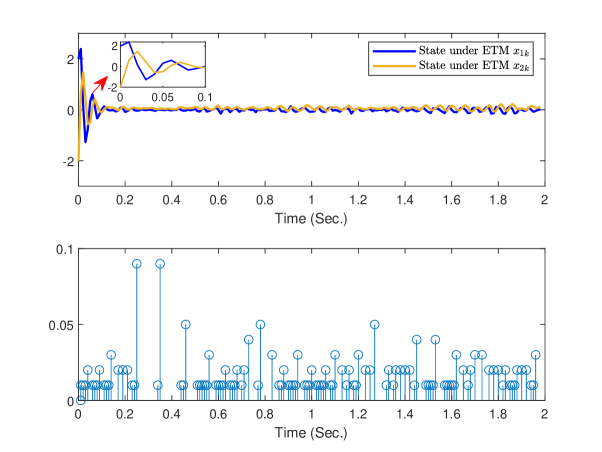
Figure 2: The state responses and inter-event intervals of event-triggered LPV systems (93) actuated by data-driven controller (90).

In what follows, we aim to perform two examples to validate the effectiveness of Procedure 2. Example 4.23 corresponds to the scenarios of one-dimension output tracking, while Example 4.24 corresponds to the plane output tracking, which are potentially utilized for robotic motion control.

Example 4.23.

We consider the augmented LPV systems (137) with the correspond dimensions $\bar{n}\hskip-1.99997pt=\hskip-1.99997pt2$, $m\hskip-1.99997pt=\hskip-1.99997pt1$, and $\ell\hskip-1.99997pt=\hskip-1.99997pt1$. Then, the system parameters embedded in (142) are prescribed by

$$\hskip-6.00006pt\widehat{A}_{d0} \hskip-8.00003pt=\hskip-8.00003pt \hskip-1.99997pt\left[\hskip-1.99997pt\begin{array}[]{cc}\hskip-1.99997pt0.3023\hskip-1.99997pt&\hskip-1.99997pt0.0000\\ \hskip-1.99997pt0.1885\hskip-1.99997pt&\hskip-1.99997pt1.0000\end{array}\hskip-1.99997pt\right],\widehat{A}_{d1}\hskip-1.99997pt=\hskip-3.00003pt\left[\hskip-1.99997pt\begin{array}[]{cc}\hskip-1.99997pt0.5469\hskip-1.99997pt&\hskip-1.99997pt0.0000\\ \hskip-1.99997pt0.0997\hskip-1.99997pt&\hskip-1.99997pt0.0000\end{array}\hskip-1.99997pt\right],$$

$$\hskip-6.00006pt\widehat{B}_{d0}^{\top} \hskip-8.00003pt=\hskip-8.00003pt \hskip-1.99997pt\left[\hskip-1.99997pt\begin{array}[]{cc}\hskip-1.99997pt0.9902\hskip-1.99997pt&\hskip-1.99997pt0.9672\end{array}\hskip-1.99997pt\right],\widehat{B}_{d1}^{\top}\hskip-1.99997pt=\hskip-3.00003pt\left[\hskip-1.99997pt\begin{array}[]{cc}\hskip-1.99997pt0.6914\hskip-1.99997pt&\hskip-1.99997pt0.0470\end{array}\hskip-1.99997pt\right].$$

Besides, we represent the scheduling signal set with the form $\mathds{P}\hskip-1.99997pt=\hskip-1.99997pt[-1,1]$. Along the execution steps of Procedure 2, we have the length $\widehat{\mathcal{T}}$ of data collection satisfying $\widehat{\mathcal{T}}\hskip-1.99997pt\geq\hskip-1.99997pt11$, and set $\widehat{\mathcal{T}}\hskip-1.99997pt=\hskip-1.99997pt17$ in practice, such that $\mathrm{Rank}(\widehat{\Theta})=6$ satisfies Lemma 3.12. We choose $\varepsilon_{3}\hskip-1.99997pt=\hskip-1.99997pt0.01$, $\hat{\sigma}\hskip-1.99997pt=\hskip-1.99997pt4$ and $\beta_{3}\hskip-1.99997pt=\hskip-1.99997pt0.2$ in Theorem 3.14, then solving the semidefinite programming in Theorem 3.16 leads to $P=\mathrm{Col}([0.0692,-0.0210],[-0.0210,0.0559])$, acting as a feasible solution for control gain scheduling. To eliminate the numerical conditioning problem in terms of the reversion of $P$, we supplement the condition $0.1\hskip-1.99997pt\leq\hskip-1.99997pt\mathrm{Trace}(P)\hskip-1.99997pt\leq\hskip-1.99997pt10$ when executing Procedure 2. We define $\hat{\mu}=9$, $\varepsilon_{4}=0.001$, $\beta_{4}=\beta_{3}/2=0.1$ in Theorem 3.14 and $\hat{v}\hskip-1.99997pt=\hskip-1.99997pt20$ in the triggering logic (183). Based on the feasible $P$ and $F_{Q}$, we can obtain the triggering gains

$$\hskip-6.00006pt\widehat{\Psi}_{1} \hskip-8.00003pt=\hskip-8.00003pt \hskip-1.99997pt\left[\hskip-1.99997pt\begin{array}[]{cc}\hskip-1.99997pt550.3198\hskip-1.99997pt&\hskip-1.99997pt260.2914\\ \hskip-1.99997pt260.2914\hskip-1.99997pt&\hskip-1.99997pt991.6524\end{array}\hskip-1.99997pt\right]\hskip-1.99997pt,\widehat{\Psi}_{2}\hskip-1.99997pt=\hskip-3.00003pt\left[\hskip-1.99997pt\begin{array}[]{cc}\hskip-1.99997pt0.2990\hskip-1.99997pt&\hskip-1.99997pt0.0534\\ \hskip-1.99997pt0.0534\hskip-1.99997pt&\hskip-1.99997pt0.2027\end{array}\hskip-1.99997pt\right]\hskip-3.00003pt.$$

Hence, we set the time horizon bound $T_{I}=6s$ and the initial state $\boldsymbol{\psi}_{0}=\mathrm{Col}(1,1)$, and generate the perturbation signal $\boldsymbol{\omega_{k}}$ in an random way satisfying $\|\boldsymbol{\boldsymbol{\varpi}_{k}}\|\hskip-1.99997pt\leq\hskip-1.99997pt\hat{\delta}=1.01$. Within this example, we consider two representative one-dimension signal to conduct the robust trajectory tracking simulations. First, we consider a sinusoidal signal $\hskip-1.00006pt\boldsymbol{r}_{k}\hskip-1.99997pt=\hskip-1.99997pt\sin(4hk),h\hskip-1.99997pt=\hskip-1.99997pt2\pi T_{I}/k_{\mathrm{step}}$ and obtain the tracking responses of closed-loop LPV system and the inter-event intervals of event-triggered LPV controller, that are illustrated by Fig. 3. Besides, we consider the square-wave signal $\hskip-1.00006pt\boldsymbol{r}_{k}$, whose minimum and maximum values are $-1$ and $1$, respectively, and obtain the tracking responses of closed-loop LPV system and the inter-event intervals of event-triggered LPV controller, that are illustrated by Fig. 4. Accordingly, the effectiveness of Procedure 2, corresponding to event-triggered robust tracking of scalar signals for LPV systems from data, can be validate by this example.

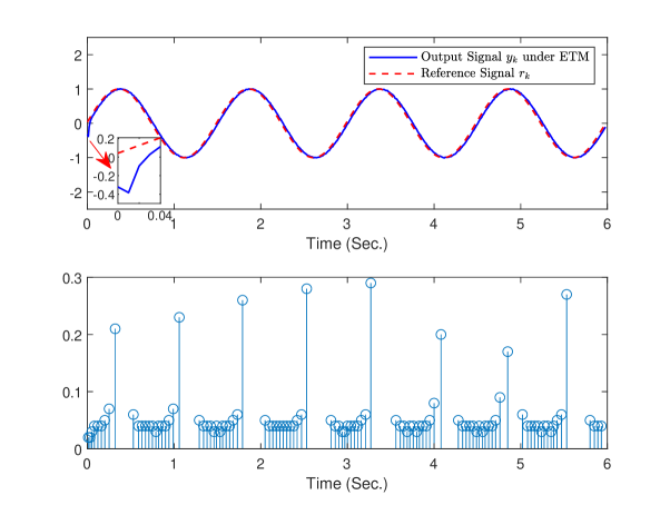
Figure 3: The robust tracking responses and inter-event intervals of event-triggered LPV systems (137) actuated by data-driven controller (176)-Case 1: sinusoidal reference signal.

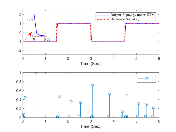
Figure 4: The robust tracking responses and inter-event intervals of event-triggered LPV systems (137) actuated by data-driven controller (176)-Case 2: square-wave signal reference signal.

Example 4.24.

We consider the augmented LPV systems (137) with the correspond dimensions $\bar{n}\hskip-1.99997pt=\hskip-1.99997pt3$, $m\hskip-1.99997pt=\hskip-1.99997pt2$, and $\ell\hskip-1.99997pt=\hskip-1.99997pt1$. Then, the system parameters embedded in (142) are prescribed by

$$\hskip-6.00006pt\widehat{A}_{d0} \hskip-8.99994pt=\hskip-8.99994pt \hskip-1.99997pt\left[\hskip-1.99997pt\begin{array}[]{ccc}\hskip-1.99997pt0.5387\hskip-1.99997pt&\hskip-1.99997pt0.0000\hskip-1.99997pt&\hskip-1.99997pt0.0000\\ \hskip-1.99997pt0.2466\hskip-1.99997pt&\hskip-1.99997pt1.0000\hskip-1.99997pt&\hskip-1.99997pt0.0000\\ \hskip-1.99997pt0.3765\hskip-1.99997pt&\hskip-1.99997pt0.0000\hskip-1.99997pt&\hskip-1.99997pt1.0000\end{array}\hskip-1.99997pt\right]\hskip-3.00003pt,\widehat{B}_{d0}\hskip-1.99997pt=\hskip-3.00003pt\left[\hskip-1.99997pt\begin{array}[]{cc}\hskip-1.99997pt0.5450\hskip-1.99997pt&\hskip-1.99997pt0.2260\\ \hskip-1.99997pt0.6290\hskip-1.99997pt&\hskip-1.99997pt0.0160\\ \hskip-1.99997pt0.9022\hskip-1.99997pt&\hskip-1.99997pt0.9636\end{array}\hskip-1.99997pt\right]\hskip-3.00003pt,$$

$$\hskip-6.00006pt\widehat{A}_{d0} \hskip-8.99994pt=\hskip-8.99994pt \hskip-1.99997pt\left[\hskip-1.99997pt\begin{array}[]{ccc}\hskip-1.99997pt0.8871\hskip-1.99997pt&\hskip-1.99997pt0.0000\hskip-1.99997pt&\hskip-1.99997pt0.0000\\ \hskip-1.99997pt0.8401\hskip-1.99997pt&\hskip-1.99997pt0.0000\hskip-1.99997pt&\hskip-1.99997pt0.0000\\ \hskip-1.99997pt0.8190\hskip-1.99997pt&\hskip-1.99997pt0.0000\hskip-1.99997pt&\hskip-1.99997pt0.0000\end{array}\hskip-1.99997pt\right]\hskip-3.00003pt,\widehat{B}_{d0}\hskip-1.99997pt=\hskip-3.00003pt\left[\hskip-1.99997pt\begin{array}[]{cc}\hskip-1.99997pt0.5289\hskip-1.99997pt&\hskip-1.99997pt0.2227\\ \hskip-1.99997pt0.2676\hskip-1.99997pt&\hskip-1.99997pt0.8512\\ \hskip-1.99997pt0.7303\hskip-1.99997pt&\hskip-1.99997pt0.4969\end{array}\hskip-1.99997pt\right]\hskip-3.00003pt.$$

Besides, we represent the scheduling signal set with the form $\mathds{P}\hskip-1.99997pt=\hskip-1.99997pt[-1,1]$. Along the execution steps of Procedure 2, we have the length $\widehat{\mathcal{T}}$ of data collection satisfying $\widehat{\mathcal{T}}\hskip-1.99997pt\geq\hskip-1.99997pt29$, and set $\widehat{\mathcal{T}}\hskip-1.99997pt=\hskip-1.99997pt29$ in practice, such that $\mathrm{Rank}(\widehat{\Theta})=10$ satisfies Lemma 3.12. We choose $\varepsilon_{3}\hskip-1.99997pt=\hskip-1.99997pt0.0001$, $\hat{\sigma}\hskip-1.99997pt=\hskip-1.99997pt4$ and $\beta_{3}\hskip-1.99997pt=\hskip-1.99997pt0.5$ in Theorem 3.14, then solving the semidefinite programming in Theorem 3.16 leads to a feasible solution

$$\hskip-6.00006ptP \hskip-8.99994pt=\hskip-8.99994pt \hskip-1.99997pt\left[\hskip-1.99997pt\begin{array}[]{ccc}\hskip-1.99997pt0.0486\hskip-1.99997pt&\hskip-1.99997pt-0.0022\hskip-1.99997pt&\hskip-1.99997pt-0.0065\\ \hskip-1.99997pt-0.0022\hskip-1.99997pt&\hskip-1.99997pt0.0248\hskip-1.99997pt&\hskip-1.99997pt0.0000\\ \hskip-1.99997pt-0.0065\hskip-1.99997pt&\hskip-1.99997pt0.0000\hskip-1.99997pt&\hskip-1.99997pt0.0266\end{array}\hskip-1.99997pt\right]\hskip-3.00003pt.$$

To eliminate the numerical conditioning problem in terms of the reversion of $P$, we supplement $0.1\hskip-1.99997pt\leq\hskip-1.99997pt\mathrm{Trace}(P)\hskip-1.99997pt\leq\hskip-1.99997pt10$ while executing Procedure 2. We define $\hat{\mu}=15$, $\varepsilon_{4}=0.001$, $\beta_{4}=\beta_{3}/2=0.1$ in Theorem 3.14 and $\hat{v}\hskip-1.99997pt=\hskip-1.99997pt500$ in the triggering logic (183). Based on the feasible $P$ and $F_{Q}$, we can obtain the triggering gains

$$\hskip-6.00006pt\widehat{\Psi}_{1} \hskip-8.00003pt=\hskip-8.00003pt \hskip-1.99997pt\left[\hskip-1.99997pt\begin{array}[]{ccc}\hskip-1.99997pt24081\hskip-1.99997pt&\hskip-1.99997pt4135.3\hskip-1.99997pt&\hskip-1.99997pt12237\\ \hskip-1.99997pt4153.3\hskip-1.99997pt&\hskip-1.99997pt6953.3\hskip-1.99997pt&\hskip-1.99997pt-2002.4\\ \hskip-1.99997pt12237\hskip-1.99997pt&\hskip-1.99997pt-2002.4\hskip-1.99997pt&\hskip-1.99997pt6577.3\end{array}\hskip-1.99997pt\right]\hskip-1.99997pt,$$

$$\hskip-6.00006pt\widehat{\Psi}_{2} \hskip-8.00003pt=\hskip-8.00003pt \hskip-1.99997pt\left[\hskip-1.99997pt\begin{array}[]{ccc}\hskip-1.99997pt41.4812\hskip-1.99997pt&\hskip-1.99997pt-1.9599\hskip-1.99997pt&\hskip-1.99997pt-5.5875\\ \hskip-1.99997pt-1.9599\hskip-1.99997pt&\hskip-1.99997pt20.5169\hskip-1.99997pt&\hskip-1.99997pt-1.0563\\ \hskip-1.99997pt-5.5875\hskip-1.99997pt&\hskip-1.99997pt-1.0563\hskip-1.99997pt&\hskip-1.99997pt19.9919\end{array}\hskip-1.99997pt\right]\hskip-1.99997pt.$$

Hence, setting the time horizon bound $T_{I}=30s$ and producing the perturbation signal $\boldsymbol{\omega_{k}}$ in an random way, which leads to the augmented perturbation $\boldsymbol{\varpi}_{k}$ satisfying $\|\boldsymbol{\varpi_{k}}\|\hskip-1.99997pt\leq\hskip-1.99997pt\hat{\delta}\hskip-1.99997pt=2.51$ for two different cases $\boldsymbol{r}_{k}\hskip-1.99997pt=\hskip-1.99997pt\mathrm{Col}(\boldsymbol{x}_{r,k},\boldsymbol{y}_{r,k})$. First, we consider a circle reference trajectory $\boldsymbol{x}_{r,k}^{2}\hskip-1.99997pt+\hskip-1.99997pt\boldsymbol{y}_{r,k}^{2}\hskip-1.99997pt=\hskip-1.99997pt2.5^{2}$. The initial value of augmented state in (137) is specified by $\boldsymbol{\psi}_{0}\hskip-1.99997pt=\hskip-1.99997pt\mathrm{Col}(\boldsymbol{x}_{0},\boldsymbol{\chi}_{0})\hskip-1.99997pt=\mathrm{Col}(3,-2,3)$. Accordingly, we can obtain the circle reference tracking responses of closed-loop LPV systems and the inter-event intervals of event-triggered mechanism (183) illustrated by Subfig. 5(a)-5(d). Besides, we consider a shape-$8$ reference trajectory $\boldsymbol{y}_{k}\hskip-1.99997pt=\hskip-1.99997pt2\boldsymbol{x}_{k}f_{q}(\boldsymbol{x}_{k})$ with $f_{q}(\boldsymbol{x}_{k})\hskip-1.99997pt=\hskip-1.99997pt\sqrt{1\hskip-1.99997pt-\hskip-1.99997pt(\boldsymbol{x}_{k}/2.5)^{2}}$. The initial value of augmented state in (137) is prescribed by $\boldsymbol{\psi}_{0}\hskip-1.99997pt=$ $\mathrm{Col}(\boldsymbol{x}_{0},\boldsymbol{\chi}_{0})\hskip-1.99997pt=\hskip-1.99997pt\mathrm{Col}(1,1,1)$. We obtain the tracking responses of closed-loop LPV systems and inter-event intervals of event-triggered mechanism (183) illustrated by Subfig. 5(e)-5(h). With regard to Fig. 5, we separate the simulation time horizon into three parts, that is, T1($0-10s$), T2($10-20s$), and T3($20-30s$), to clearly mirror the plane tracking responses. Therefore, the effectiveness of Procedure 2, corresponding to event-triggered robust tracking of plane trajectories for LPV systems from data, can be validate by this example.

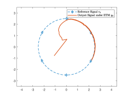
(a) The circle trajectory (T1)

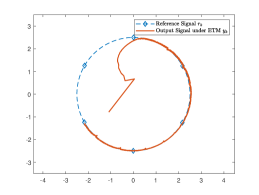
(b) The circle trajectory (T2)

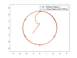
(c) The circle trajectory (T3)

(d) The event-trigger instants

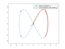
(e) The shape-8 trajectory (T1)

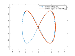
(f) The shape-8 trajectory (T2)

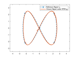
(g) The shape-8 trajectory (T3)

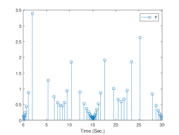
(h) The event-trigger instants

Figure 5: The robust tracking responses and inter-event intervals of event-triggered LPV systems (137) actuated by data-driven controller (176)-Case 1: circle reference and Case 2: shape-8 reference.

5 Conclusion

This paper has investigated event-triggered robust stabilization and reference tracking control strategies for LPV systems from available data. First, we established the condition of $\theta$-persistence of excitation for LPV systems, which acts as the prerequisite of direct data-driven LPV control synthesis. Then, for the perturbed LPV systems, we explored the sufficient data-dependent conditions on ensuring the closed-loop stability and established the convex programmings for control synthesis in view of Petersen’s lemma and full-block S-procedure. Besides, we developed an event-triggered mechanism and connected the triggering parameters with stability certificates, leading to the feasible data-driven event-triggered LPV control procedure. In addition, we extended the theoretical results to the scenario of robust reference tracking, with the aid of integral compensator, and synthesized the feasible data-driven event-triggered LPV tracking controller. Finally, we performed a group of numerical simulations to verify the effectiveness and the applicability of our theoretical derivations herein.

References

References

- [1] J. Mohammadpour and C. W. Scherer, Control of Linear Parameter Varying Systems with Applications. Springer Science & Business Media, 2012.
- [2] T. Martin, T. B. Schn, and F. Allgwer, ”Guarantees for data-driven control of nonlinear systems using semidefinite programming: A survey”, Annual Reviews in Control, vol. 56, num. 100911, 2023.
- [3] X. Ping, J. Yao, B. Ding, and Z. Li, ”Tube-based output feedback robust MPC for LPV systems with scaled terminal constraint sets”, IEEE Transactions on Cybernetics, vol. 52, no. 8, pp. 7563-7576, 2022.
- [4] A. P. Pandey and M. C. de Oliveira, ”A new discrete-time stabilizability condition for linear parameter-varying systems”, Automatica, vol. 79, pp. 214-217, 2017.
- [5] A. N. Vargas, C. M. Agulhari, R. C. L. F. Oliveira, and V. M. Preciado, ”Robust stability analysis of linear parameter-varying systems with Markov jumps”, IEEE Transactions on Automatic Control, vol. 67, no. 11, pp. 6234-6239, 2022.
- [6] P. B. Cox, S. Weiland, and R. Tth, ”Affine parameter-dependent Lyapunov functions for LPV systems with affine dependence”, IEEE Transactions on Automatic Control, vol. 63, no. 11, pp. 3865-3872, 2018.
- [7] J. A. Gallegos and K. A. Barbosa, ”Set-theoretical stability analysis of LPV systems via Minkowski-Lyapunov functions”, IEEE Transactions on Automatic Control, DOI: 10.1109/TAC.2024.3441325.
- [8] S. K. Mulagaleti, M. Mejari, and A. Bemporad, ”Parameter-dependent robust control invariant sets for LPV systems with bounded parameter-variation rate”, IEEE Transactions on Automatic Control, DOI: 10.1109/TAC.2024.3454528.
- [9] J. Cheng, M. Wu, F. Wu, C. Lu, X. Chen, and W. Cao, ”Modeling and control of drill-string system with stick-slip vibrations using LPV technique”, IEEE Transactions on Control Systems Technology, vol. 29, no. 2, pp. 718-730, 2021.
- [10] P. Polcz, B. Kulcsar, T. Peni, and G. Szederkenyi, ”Passivity analysis of rational LPV systems using Finsler’s lemma”, in IEEE 58th Conference on Decision and Control, pp. 3793-3798, 2019.
- [11] C. E. de Souza, K. A. Barbosa, and A. T. Neto, ”Robust filtering for discrete-time linear systems with uncertain time-varying parameters”, IEEE Transactions on Signal Processing, vol. 54, no. 6, pp. 2110-2118, 2006.
- [12] G. Cai, T. Wu, M. Hao, H. Liu, and B. Zhou, ”Dynamic event-triggered gain-scheduled control for a polytopic LPV model of morphing aircraft”, IEEE Transactions on Aerospace and Electronic Systems, vol. 61, no. 1, pp. 93-106, 2025.
- [13] T. J. Meijer, V. Dolk, and W. P. M. H. Heemels, ”Certificates of nonexistence for analyzing stability, stabilizability and detectability of LPV systems”, Automatica, vol. 170, num. 111841, 2024.
- [14] J. C. Willems, P. Rapisarda, I. Markovsky, and B. L. M. De Moor, ”A note on persistency of excitation”, Systems & Control Letters, vol. 54, pp. 325-329, 2005.
- [15] K. He, S. Shi, T. van den Boom, and B. De Schutter, ”From learning to safety: A direct data-driven framework for constrained control”, arXiv Preprint, arXiv: 2505.15515v1.
- [16] W. Liu, G. Wang, J. Sun, F. Bullo, and J. Chen, ”Learning robust data-based LQG controllers from noisy data”, IEEE Transactions on Automatic Control, vol. 69, no. 12, pp. 8526-8538, 2024.
- [17] C. De Persis and P. Tesi, ”Formulas for data-driven control: Stabilization, optimality, and robustness”, IEEE Transactions on Automatic Control, vol. 65, no. 3, pp. 909-924, 2020.
- [18] F. Drfler, P. Tesi, and C. De Persis, ”On the certainty-equivalence approach to direct data-driven LQR design”, IEEE Transactions on Automatic Control, vol. 68, no. 12, pp. 7989-7996, 2023.
- [19] J. Berberich, J. Khler, M. A. Mller, and F. Allgwer, ”Data-driven model predictive control with stability and robustness guarantees”, IEEE Transactions on Automatic Control, vol. 66, no. 4, pp. 1702-1717, 2021.
- [20] Z. Ren, H. Liu, G. Wen, and J. L, ”Event-triggered data-driven security formation control for quadrotors under denial-of-service attacks and communication faults”, IEEE Transactions on Cybernetics, DOI: 10.1109/TCYB.2024.3467178.
- [21] J. Wang, J. Sun, J. Yang, and S. Li, ”Periodic event-triggered model predictive control for networked nonlinear uncertain systems with disturbances”, IEEE Transactions on Cybernetics, vol. 54, no. 12, pp. 7501-7513, 2024.
- [22] R. Ma, P. Shi, and L. Wu, ”Sparse false injection attacks reconstruction via descriptor sliding mode observers”, IEEE Transactions on Automatic Control, vol. 66, no. 11, pp. 5369-5376, 2021.
- [23] T. An, B. Dong, H. Yan, L. Liu, and B. Ma, ”Dynamic event-triggered strategy-based optimal control of modular robot manipulator: A multiplayer nonzero-sum game perspective”, IEEE Transactions on Cybernetics, vol. 54, no. 12, pp. 7514-7526, 2024.
- [24] M. Rotulo, C. De Persis, and P. Tesi, ”Online learning of data-driven controllers for unknown switched linear systems”, Automatica, vol. 145, num. 110519, 2022.
- [25] J.Berberich, C. W. Scherer, and F. Allgwer, ”Combining prior knowledge and data for robust controller design”, IEEE Transactions on Automatic Control, vol. 68, no. 8, pp. 4618-4633, 2023.
- [26] H. J. van Waarde, M. K. Camlibel, and M. Mesbahi, ”From noisy data to feedback controllers: Nonconservative design via a matrix S-lemma”, IEEE Transactions on Automatic Control, vol. 67, no. 1, pp. 162-175, 2022.
- [27] A. Bisoffi, C. De Persis, and P. Tesi, ”Data-driven control via Petersen’s lemma”, Automatica, vol. 145, num. 110537, 2022.
- [28] C. De Persis, M. Rotulo, and P. Tesi, ”Learning controllers from data via approximate nonlinearity cancellation”, IEEE Transactions on Automatic Control, vol. 68, no. 10, pp. 6082-6097, 2023.
- [29] T. Dai and M. Sznaier, ”A semi-algebraic optimization approach to data-driven control of continuous-time nonlinear systems”, IEEE Control Systems Letters, vol. 5, no. 2, pp. 487-492, 2021.
- [30] A. Koch, J. Berberich, and F. Allgwer, ”Provably robust verification of dissipativity properties from data”, IEEE Transactions on Automatic Control, vol. 67, no. 8, pp. 4248-4255, 2022.
- [31] A. Bisoffi, C. De Persis, and P. Tesi, ”Learning controllers for performance through LMI regions”, IEEE Transactions on Automatic Control, vol. 68, no. 7, pp. 4351-4358, 2023.
- [32] L. Li, C. De Persis, P. Tesi, and N. Monshizadeh, ”Data-based transfer stabilization in linear systems”, IEEE Transactions on Automatic Control, vol. 69, no. 3, pp. 1866-1873, 2024.
- [33] R. Strsser, M. Schaller, K. Worthmann, J. Berberich, and F. Allgwer, ”Koopman-based feedback design with stability guarantees”, IEEE Transactions on Automatic Control, vol. 70, no. 1, pp. 355-370, 2025.
- [34] A. Koch, J. Berberich, J. Khler, and F. Allgwer, ”Determining optimal input-output properties: A data-driven approach”, Automatica, vol. 134, num. 109906, 2021.
- [35] M. Bianchi, S. Grammatico, and J. Corts, ”Data-driven stabilization of switched and constrained linear systems”, Automatica, vol. 171, num. 111974, 2025.
- [36] G. Disar and M. E. Valcher, ”On the equivalence of model-based and data-driven approaches to the design of unknown-input observers”, IEEE Transactions on Automatic Control, vol. 70, no. 3, pp. 2074-2081, 2025.
- [37] C. De Persis, R. Postoyan, and P. Tesi, ”Event-triggered control from data”, IEEE Transactions on Automatic Control, vol. 69, no. 6, pp. 3780-3795, 2024.
- [38] H. Zhou, Y. Zuo, and S. Tong, ”Fuzzy adaptive event-triggered consensus control for nonlinear multiagent systems under jointly connected switching networks”, IEEE Transactions on Cybernetics, vol. 54, no. 12, pp. 7163-7172, 2024.
- [39] C. Liu, Z. Chu, Z. Duan, H. Zhang, and Z. Ma, ”Decentralized event-triggered tracking control for unmanned interconnected systems via particle swarm optimization-based adaptive dynamic programming”, IEEE Transactions on Cybernetics, vol. 54, no. 11, pp. 6895-6909, 2024.
- [40] S. Wildhagen, J. Berberich, M. Hertneck, and F. Allgwer, ”Data-driven analysis and controller design for discrete-time systems under aperiodic sampling”, IEEE Transactions on Automatic Control, vol. 68, no. 6, pp. 3210-3225, 2023.
- [41] C. Verhoek, J. Berberich, S. Haesaert, F. Allgwer, and R. Tth, ”Data-driven dissipativity analysis of linear parameter-varying systems”, IEEE Transactions on Automatic Control, vol. 69, no. 12, pp. 8603-8616, 2024.
- [42] C. Verhoek, R. Tth, and H. S. Abbas, ”Direct data-driven state-feedback control of linear parameter-varying systems”, arXiv Preprint, arXiv: 2211.17182v4.
- [43] C. Verhoek, I. Markovsky, S. Haesaert, and R. Tth, ”The behavioral approach for LPV data-driven representations”, arXiv Preprint, arXiv: 2412.18543v1.
- [44] H. S. Abbas, R. Tth, N. Meskin, J. Mohanmadpour, and J. Hanema, ”A robust MPC for input-output LPV models”, IEEE Transactions on Automatic Control, vol. 61, no. 12, pp. 4183-4188, 2016.
- [45] A. Golabi, N. Meskin, R. Tth, J. Mohammadpour, and T. Donkers, ”Event-triggered control for discrete-time linear parameter-varying systems”, in 2016 American Control Conference, pp. 3680-3685, 2016.
- [46] J. Clouson, H. van Waarde, and F. Drfler, ”Robust fundamental lemma for data-driven control”, arXiv Preprint, arXiv: 2205.06636.
- [47] V. Digge and R. Pasumarthy, ”Data-driven event-triggered control for discrete-time LTI systems”, in 2022 European Control Conference, pp. 1355-1360,
- [48] C. W. Scherer, ”LPV control and full block multipliers”, Automatica, vol. 37, pp. 361-375, 2001.
- [49] J. Lfberg, ”YALMIP: A toolbox for modeling and optimization in MATLAB”, in 2004 IEEE International Confernece on Robotics and Automation, pp. 284-289, 2004.
- [50] M. ApS, Mosek Optimization Toolbox for Matlab, User’s Guide and Reference Manual, Version 4, [Online] https://www.mosek.com/, 2019.